Embed Size (px)
Citation preview

This pdf consists of four parts. First, the original paper (including an erratum) by Monique de Jager and colleagues:
Second, the associated supporting online material:
Third, a comment on the paper by Vincent Jansen and colleagues:
And fourth, the response of Monique de Jager and colleagues to these comments:

4. V. B. Polyakov, R. N. Clayton, J. Horita, S. D. Mineev,Geochim. Cosmochim. Acta 71, 3833 (2007).
5. I. B. Butler, C. Archer, D. Vance, A. Oldroyd, D. Rickard,Earth Planet. Sci. Lett. 236, 430 (2005).
6. Y. Duan et al., Earth Planet. Sci. Lett. 290, 244 (2010).7. C. M. Johnson, B. L. Beard, E. E. Roden, Annu. Rev. Earth
Planet. Sci. 36, 457 (2008).8. C. Archer, D. Vance, Geology 34, 153 (2006).9. R. Raiswell, D. E. Canfield, Am. J. Sci. 298, 219 (1998).
10. J. L. Skulan, B. L. Beard, C. M. Johnson, Geochim.Cosmochim. Acta 66, 2995 (2002).
11. A. D. Anbar, O. Rouxel, Annu. Rev. Earth Planet. Sci. 35,717 (2007).
12. Materials and methods and detailed results are availableas supporting material on Science Online.
13. D. Rickard, G. W. Luther III, Geochim. Cosmochim. Acta61, 135 (1997).
14. G. W. Luther III, D. Rickard, J. Nanopart. Res. 7, 389(2005).
15. D. Rickard, G. W. Luther 3rd, Chem. Rev. 107, 514(2007).
16. E. A. Schauble, Rev. Mineral. Geochem. 55, 65 (2004).
17. A. D. Anbar, J. E. Roe, J. Barling, K. H. Nealson, Science288, 126 (2000).
18. I. B. Butler, M. E. Bottcher, D. Rickard, A. Oldroyd,Earth Planet. Sci. Lett. 228, 495 (2004).
19. A. E. Isley, J. Geol. 103, 169 (1995).20. K. E. Yamaguchi, C. M. Johnson, B. L. Beard, H. Ohmoto,
Chem. Geol. 218, 135 (2005).21. R. Guilbaud, I. B. Butler, R. M. Ellam, D. Rickard,
A. Oldroyd, Geochim. Cosmochim. Acta 75, 2721 (2011).22. A. D. Czaja et al., Earth Planet. Sci. Lett. 292, 170
(2010).23. D. E. Canfield, Annu. Rev. Earth Planet. Sci. 33,
1 (2005).24. S. W. Poulton, P. W. Fralick, D. E. Canfield, Nat. Geosci.
3, 486 (2010).25. D. E. Canfield, Nature 396, 450 (1998).26. C. Li et al., Science 328, 80 (2010); 10.1126/
science.1182369.27. A. McAnena, S. Severmann, S. W. Poulton, Geochim.
Cosmochim. Acta 73, A854 (2009).28. C. M. Johnson, E. E. Roden, S. A. Welch, B. L. Beard,
Geochim. Cosmochim. Acta 69, 963 (2005).
29. S. Severmann, T. W. Lyons, A. Anbar, J. McManus,G. Gordon, Geology 36, 487 (2008).
30. O. J. Rouxel, M. Auro, Geostand. Geoanal. Res. 34, 135(2010).
Acknowledgments: This work was funded by an ECOSSEPh.D. studentship to R.G. and Natural EnvironmentResearch Council research grant NE/E003958/1 toI.B.B. We are thankful to K. Keefe, V. Gallagher,N. Odling, B. D. Roach, S. Mowbray, and C. Frickefor technical support and B. Ngwenya, A. Matthews,D. Rickard, A. McAnena, and M. Pękala forconstructive discussions.
Supporting Online Materialwww.sciencemag.org/cgi/content/full/332/6037/1548/DC1Materials and MethodsFig. S1Table S1References (31–41)
17 January 2011; accepted 17 May 201110.1126/science.1202924
Lévy Walks Evolve ThroughInteraction Between Movement andEnvironmental ComplexityMonique de Jager,1* Franz J. Weissing,2 Peter M. J. Herman,1
Bart A. Nolet,3,4 Johan van de Koppel1,4
Ecological theory predicts that animal movement is shaped by its efficiency of resource acquisition.Focusing solely on efficiency, however, ignores the fact that animal activity can affect resourceavailability and distribution. Here, we show that feedback between individual behavior andenvironmental complexity can explain movement strategies in mussels. Specifically, experimentsshow that mussels use a Lévy walk during the formation of spatially patterned beds, and modelsreveal that this Lévy movement accelerates pattern formation. The emergent patterning in musselbeds, in turn, improves individual fitness. These results suggest that Lévy walks evolved as a resultof the selective advantage conferred by autonomously generated, emergent spatial patterns inmussel beds. Our results emphasize that an interaction between individual selection and habitatcomplexity shapes animal movement in natural systems.
Animals must face the daunting complex-ity of the natural world when searchingfor food, shelter, and other resources cru-
cial for survival. To cope with the challenge tomaximize the probability of resource encounters,many organisms adopt specialized search strat-egies (1, 2) that can be described by randomwalks. Brownian and Lévy walks are prominentexamples of random walk strategies where boththe direction and step length of the constituentmoves are drawn from a probability distribution
(1–4). These movement patterns differ in thedistribution of step lengths, which are derivedfrom an exponential distribution in the case ofBrownian motion, but follow a power-law dis-tribution in case of Lévy motion (4–7), wheremany short steps are occasionally alternated witha long step. Model simulations have shown that aLévy walk provides faster dispersal (2, 3), morenewly visited sites (1, 2), and less intraspecificcompetition than Brownian walks (4); it is there-fore considered the most efficient random searchstrategy in resource-limited environments wherefood occurs patchily at locations unknown to the
searcher (1–3) and, most importantly, where theresource distribution is largely unaffected by the ac-tivities of the searching animal (8, 9). Althoughshown to be optimal for only these specific con-ditions, Lévy walks are broadly found in nature(1, 10–12), suggesting that they are adaptive overa wider range of conditions. To explain this wideoccurrence, we hypothesize that organisms them-selves affect the availability and spatial distri-bution of the resources upon which they depend(13). Consequently, the movement strategies oforganisms can shape the environment.
On intertidal flats, the distribution of regularlyspaced clumps of mussels (Mytilus edulis) resultsfrom the interaction between local mussel densityand the crawling movement of young mussels(5, 14, 15). In particular, pattern formation inmussel beds is attributable to two opposingmech-anisms: cooperation and competition (16). Bymoving into cooperative aggregations, musselsincrease their local density, which decreaseswave stress and predation risk. Conversely, com-petition for algae, which occurs on a larger spatialscale than facilitation, prevents the formation oflarger clumps by limiting the number of musselswithin a long range. The interaction of local fa-cilitation and long-range competition results inthe emergence of a patchy distribution of indi-viduals, which simultaneously reduces risk andminimizes competition for algae (15). Hence, inthis system, the distribution of suitable settling lo-cations, an important resource for mussels, is de-termined by the existing distribution of mussels,which develops in response to the movement ofits comprising individuals. Here, we investigate
1Spatial Ecology Department, Netherlands Institute of Ecology(NIOO-KNAW), Post Office Box 140, 4400 AC Yerseke, Nether-lands. 2Theoretical Biology Group, Centre for Ecological andEvolutionary Studies, University of Groningen, Nijenborgh 7,9747 AG Groningen, Netherlands. 3Department of AnimalEcology, Netherlands Institute of Ecology (NIOO-KNAW), PostOffice Box 50, 6700 AB Wageningen, Netherlands. 4ProjectGroup Movement Ecology, Netherlands Institute of Ecology(NIOO-KNAW), Post Office Box 50, 6700 AB Wageningen,Netherlands.
*To whom correspondence should be addressed. E-mail:[email protected]
Table 1. Goodness-of-fit (G), AIC weights, adjusted R2, and Lévy exponents for three classes of movementstrategies. The observed step length distribution is best explained by a Lévy walk or a truncated Lévy walk,with Lévy exponents close to 2.
G AIC weights Adjusted R2 Lévy exponent
Truncated Lévy walk 22.45 0.443 0.997 2.01Lévy walk 47.22 0.428 0.997 2.06Brownian walk −190.09 0.129 0.837 −
www.sciencemag.org SCIENCE VOL 332 24 JUNE 2011 1551
REPORTSCORRECTED 23 DECEMBER 2011; SEE LAST PAGE
on
Feb
ruar
y 20
, 201
2w
ww
.sci
ence
mag
.org
Dow
nloa
ded
from

whether the interplay between movement strat-egy and habitat complexity results in the emer-gence of Lévy walks in these self-organizingmussel beds.
We first tested the hypothesis that musselmovement is described by a Lévy walk (or atruncated Lévy walk) against alternative modelsreported in the literature, namely, a Brownianwalkand a composite Brownian walk (17–19). We ob-served the movements of 50 mussels during theprocess of pattern formation and of 12 musselsin solitary experiments in mesocosm tanks. Steplengths were estimated by the distance betweentwo subsequent reorientation events (5). Theresulting step length distribution was comparedwith the family of power-law distributions,P(l)=Cl−m, where P(l) is the probability of a step oflength l and C is a constant ensuring that thetotal probability equals 1. The exponent m de-fines the shape of the distribution and thereforedetermines the resulting movement strategy. If1 < m < 3, the movement pattern corresponds toa Lévy walk. When m approaches 1, the move-ment is approximately ballistic, while it is approx-imately Brownian when m approaches 3 (and form > 3) (2, 5, 20) (fig. S2.2). The Lévy walksfound in nature typically have an exponent m of~2 (1, 10–12).
Our results show that mussels use a Lévywalk during the process of pattern formation. Onthe basis of maximum-likelihood estimation andthe derived goodness-of-fit (G), Akaike informa-tion criterion (AIC), and the fraction of varianceexplained by the model (R2), we found that Lévywalk and truncated Lévy walk distributions, bothwith m ≈ 2, provided the best fit to the data over arange of at least two orders of magnitude (5)(Table 1, Fig. 1, and table S3.1). A possible al-ternative explanation is that mussel movementfollows a composite Brownianwalk, wheremove-ment speeds are adjusted to local environmentalconditions (17–21). Such a strategy can have astep length distribution similar to that of a Lévywalk and is therefore often overlooked. However,when mussel movements were grouped by localmussel density (the density of mussels within aradius of 3.3 cm) and long-range density (the den-sity of mussels within a radius of 22.5 cm), steplength distributions did not differ between the den-sity categories, and mussels were found to per-form a Lévy walk with m ≈ 2, irrespective of thelocal and long-range density (5) (table S3.2).Hence, we reject the hypotheses of Brownianwalk and composite Brownian walk and con-clude that mussel movement is best described bya Lévy walk.
To examine why mussels adopt a Lévy walk,we investigated the effect of movement strategyon the rate of pattern formation by designing anindividual-based model (5). In this model, pat-terns arise by the mussels’ decisions to stay at alocation or move away from it. We used experi-mental data from a previous study to estimate theparameters of this stop-or-move behavior (5, 15)(fig. S2.2). Although step length distributions are
unaffected by mussel density, we found that theprobability that a mussel moves decreases withshort-range density (the density ofmussels withina radius of 3.3 cm) and increases with long-rangedensity (the density of mussels within a radius of22.5 cm). On the basis of these parameters, sim-ulated mussels stay in places where they can ag-gregate with direct neighbors, but move awayfrom crowded locations where food becomeslimiting. If a simulated mussel moves, the move-ment distance is randomly drawn from the power-law distribution that corresponds to its movement
strategy. For a range of movement strategies(1 < m ≤ 3), we observed the distance traveled untila pattern has formed. Operationally, we say that apattern has formed when the density of simulatedmussels within 3.3-cm distance is on average 1.5times as large as the density of mussels within22.5-cm distance of an individual. Assumingthat the movement speed is constant, the rate ofpattern formation for each movement strategyis proportional to the inverse of the average dis-tance traversed by the mussels until a pattern hasformed (5).
Fig. 1. Experimental and model results showing that mussel movement, which is best described by a Lévywalk, generates patterns in mussel beds. (A) Frequency distribution of step lengths of all solitary mussels(12 mussels, 12,401 steps). (B) Inverse cumulative frequency distribution of the step lengths. (C) Patternformation in an experimental mussel bed. (D) Pattern generated with our individual-based model.
Fig. 2. The rate of pattern forma-tion for various movement strategies.Because we assume that movementspeed is constant, we can calculatethe rate of patterning as the normal-ized inverse of the distance traverseduntil a pattern is formed. A Lévy walkwith exponent m ≈ 2 minimizes thetime needed to form a pattern.
1.0 1.5 2.0 2.5 3.0
0.0
0.2
0.4
0.6
0.8
1.0
Lévy exponent
Rat
e of
pat
tern
form
atio
n
24 JUNE 2011 VOL 332 SCIENCE www.sciencemag.org1552
REPORTS
on
Feb
ruar
y 20
, 201
2w
ww
.sci
ence
mag
.org
Dow
nloa
ded
from

Simulations reveal that movement strategiesdiffer strongly in terms of the rate at which theycreate patterns (Fig. 2). A Lévy walk with ex-ponent m ≈ 2 generated a spatially heterogeneouspatternmore rapidly than did either ballistic move-ment (m→ 1) or a Brownian walk (m→ 3). Spe-cifically, the large steps associated with a smallvalue of m prevented quick formation of tightclusters, whereas a larger value of m requiredmanysmall steps to create clustering. A Lévy walk withm ≈ 2 seems to be the optimal trade-off betweenfinding dispersed conspecifics and maintaininghigh local densities, thereby maximizing the rateof pattern development. Hence, our simulation re-sults suggest that a Lévy strategy with m ≈ 2 isoptimal for pattern formation.
Because pattern formation both improvesmus-sel survival and decreases competition betweenmussels (14), the movement strategy of individ-ual mussels is likely to be an important deter-minant of fitness. However, strategies that lead toa desirable outcome at the population level areoften not evolutionarily stable, as they can beexploited by free-riding strategies (22). To de-termine the long-term outcome of selection act-ing on mussels differing in movement strategy(i.e., their exponent m), we created a pairwiseinvasibility plot (PIP, Fig. 3) by performing anevolutionary invasibility analysis (5, 23, 24). Thevalues along the x axis of the PIP represent abroad range of hypothetical resident populations,each with a particular movement strategy char-acterized by an exponent mres. The y axis rep-resents the exponents mmut of potential mutantstrategies. The colors indicate whether a mutantstrategy mmut can successfully invade a residentstrategy mres—i.e., whether mutant individualshave a higher fitness than resident individuals inthe environment created by the resident popula-tion. Intersections between the lines separatingthe colored areas indicate the presence of anevolutionary attractor, thus predicting the out-come of selection on mussel movement strat-
egies. Fitness was given by the product of musselsurvival (which is proportional to short-rangemussel density) and fecundity (which is inverselyproportional to long-range mussel density and theenergy invested in movement) (5).
The PIP reveals that a Lévy walk with m ≈ 2 isthe unique evolutionary attractor of the system(Fig. 3) (23, 24). Specifically, a succession of in-vasion events will lead to the establishment of aresident population with m ≈ 2, and a residentpopulation with m ≈ 2 cannot be invaded by anyother movement strategy. We conclude that theLévy walk strategy observed in our experiments(Fig. 1) not only has a high patterning efficien-cy (Fig. 2) but is also an evolutionarily stablestrategy (Fig. 3).
Our study demonstrates an evolutionary feed-back between individual movement behavior andhigher-level complexity and could explain theevolution of Lévy walks in mussel beds. Ratherthan being a direct adaptation to an externallydetermined environment, Lévy movement in ourstudy was found to result from feedback betweenanimal behavior and mussel-generated environ-mental complexity. In essence, a Lévy walk withm ≈ 2 creates a spatial environment in which justthis movement strategy can flourish.
Although our study addresses a specific sys-tem, the assumption that search strategies canevolve through feedback between animal move-ment and environmental heterogeneity may bebroadly applicable. Such feedbacks may exist notonly in the search for conspecifics (as seen herein mussels) but also in the search for resourcesshared with conspecifics, because resource pat-terns reflect the movement patterns of their con-sumers. This applies, for instance, to the interactionbetween herbivores and vegetation, which shapesgrasslands globally (25). Additionally, feedbackbetween movement strategy and habitat com-plexity may arise when the spatial distribution ofa particular species depends on interactions witha searching organism [as in predator-prey rela-
tionships or animal-mediated seed dispersal (26)].We conclude that the interaction between animalmovement and habitat complexity is a key com-ponent in understanding the evolution of animalmovement strategies.
References and Notes1. D. W. Sims et al., Nature 451, 1098 (2008).2. F. Bartumeus, M. G. E. Da Luz, G. M. Viswanathan,
J. Catalan, Ecology 86, 3078 (2005).3. F. Bartumeus, Oikos 118, 488 (2009).4. G. M. Viswanathan et al., Physica A 282, 1 (2000).5. Materials and methods are available as supporting
material on Science Online.6. G. M. Viswanathan, Nature 465, 1018 (2010).7. E. A. Codling, M. J. Plank, S. Benhamou, J. R. Soc. Interface
5, 813 (2008).8. G. M. Viswanathan et al., Nature 401, 911 (1999).9. A. M. Reynolds, F. Bartumeus, J. Theor. Biol. 260, 98
(2009).10. G. Ramos-Fernández et al., Behav. Ecol. Sociobiol. 55,
223 (2004).11. A. M. Reynolds et al., Ecology 88, 1955 (2007).12. N. E. Humphries et al., Nature 465, 1066 (2010).13. C. G. Jones, J. H. Lawton, M. Shachak, Oikos 69, 373
(1994).14. R. A. Maas Geesteranus, Arch. Neerl. Zool. 6, 283 (1942).15. J. van de Koppel et al., Science 322, 739 (2008).16. J. van de Koppel, M. Rietkerk, N. Dankers, P. M. Herman,
Am. Nat. 165, E66 (2005).17. S. Benhamou, Ecology 88, 1962 (2007).18. A. Reynolds, Ecology 89, 2347, discussion 2351
(2008).19. S. Benhamou, Ecology 89, 2351 (2008).20. A. M. Reynolds, C. J. Rhodes, Ecology 90, 877 (2009).21. B. A. Nolet, W. M. Mooij, J. Anim. Ecol. 71, 451
(2002).22. C. Hauert, Adv. Complex Syst. 9, 315 (2006).23. S. A. H. Geritz, E. Kisdi, G. Meszena, J. A. J. Metz,
Evol. Ecol. 12, 35 (1998).24. F. Dercole, S. Rinaldi, Analysis of Evolutionary Processes:
The Adaptive Dynamics Approach and Its Applications(Princeton Univ. Press, Princeton, NJ, 2008)
25. P. Adler, D. Raff, W. Lauenroth, Oecologia 128, 465(2001).
26. D. Boyer, O. Lopez-Corona, J. Phys. A 42, 434014(2009).
Acknowledgments: For assistance, we thank S. Benhamou,A. Kölzsch, J. Powell, G. Theraulaz, W. Mooij,A. van den Berg, and J. van Soelen. We thank S. Kéfi,F. Bartumeus, B. Silliman, and M. Rietkerk for commentson manuscript drafts. M.d.J. and J.v.d.K. designed thestudy. Experimental data were collected by M.d.J. andJ.v.d.K. B.A.N. introduced the topic of Lévy walks, andF.J.W. suggested the evolutionary invasion analysis.All analyses and modeling were done by M.d.J.,assisted by J.v.d.K., P.M.J.H., and F.J.W. The paperwas written by M.d.J. and J.v.d.K., and all authorscontributed to the subsequent drafts. The authorsdeclare no competing financial interests. M.d.J. issupported by a grant from the Netherlands Organizationof Scientific Research–Earth and Life Sciences(NWO-ALW), and Project Group Movement Ecologyby the KNAW Strategic Fund. This is publication 5033of the Netherlands Institute of Ecology (NIOO-KNAW).
Supporting Online Materialwww.sciencemag.org/cgi/content/full/332/6037/1551/DC1Materials and MethodsFigs. S2.1 to S2.3Tables S3.1 and S3.2References and NotesMovie S1Matlab code for individual-based model of mussel movement(The MathWorks, Inc.)
2 December 2010; accepted 16 May 201110.1126/science.1201187
Fig. 3. Pairwise invasibility plot(PIP) indicating that the movementstrategy evolves toward a Lévy walkwith m ≈ 2. For a range of resident(x axis) and mutant (y axis) move-ment strategies, the PIP indicateswhether a mutant has a higher (red)or a lower (green) fitness than theresident and, hence, whether a mu-tant can invade the resident popu-lation (23). Here, the PIP shows thata Lévy walk with m ≈ 2 is the soleevolutionarily stable strategy (ESS).
1.0 1.5 2.0 2.5 3.0
1.0
1.5
2.0
2.5
3.0
Resident Lévy exponent
Mut
ant L
évy
expo
nent
−
+
−
+
ESS
www.sciencemag.org SCIENCE VOL 332 24 JUNE 2011 1553
REPORTS
on
Feb
ruar
y 20
, 201
2w
ww
.sci
ence
mag
.org
Dow
nloa
ded
from

1
CorreCtions & CLarifiCations
www.sciencemag.org sCiEnCE erratum post date 23 deCemBer 2011
ErratumReports: “Lévy walks evolve through interaction between movement and environmental complexity” by M. de Jager et al. (24 June, p. 1551). The statistical analysis of the mus-sel movement contained errors, which were pointed out by V. Jansen. First, the data that was used contained duplicates of a number of individuals, while other individuals had accidentally been omitted. Second, the parameter λ of the exponential distribution (which describes the Brownian walk strategy) was mistakenly estimated without considering the lower boundary of the data. Third, the AIC was estimated incorrectly, by using a least-squares rather than a maximum-likelihood calculation. Additionally, the weighed AIC was calculated incorrectly. These mistakes have been corrected using the methods of Edwards et al. [A. M. Edwards et al., Nature 449, 1044 (2007)]; the results of the new analysis are plotted in a new Fig. 1B shown here. In Fig. 1B of the original Report, a Rayleigh dis-tribution was accidentally plotted instead of an exponential distribution to describe the Brownian walk. In the statistical analysis, however, an exponential distribution was used to describe a Brownian walk. Furthermore, the movement patterns of mussels in different density treatments were reanalyzed after the comments of F. van Langevelde. The former results were found to be erroneous due to an error in the script; the scaling exponent of the movement strategy does not stay constant when mussel density increases. Although some corrections were made to the data and movement analysis, the overall conclusion of the paper that mussels adopt a Lévy walk, especially when alone, remains unchanged. We thank V. Jansen and F. van Langevelde for bringing these issues to our attention.
CorreCtions & CLarifiCations
Post date 23 December 2011
�������������������������������������������������������������������������������������������������������������������������������������������������������������������������������������������������������������������������������������������������������������������������������������������������������������������������������������������������������������������������������������������������������������������������������������������������������������������������������������������������������������������������������������������������������������������������������������������������������������������������������������������������������������������������������������������������������������������������������������������������������������������������������������������������������������������������������������������������������������������������������������������������������������������������������������������������������������������������������������������������������������������������������������������������������������������������������������������������������������������������������������������������������������������������������������������������������������������������������������������������������������������������������������������������������������������������������������������������������������������������������������������������������������������������������������������������������������������������������������������������������������������������������������������������������������������������������������������������������������������������������������������������������������������������������������������������������������������������������������������������������������������������������������������������������������������������������������������������������������������������������������������������������������������������������������������������������������������������������������������������������������������������������������������������������������������������������������������������������������������������������������������������������������������������������������������������������������������������������������������������������������������������������������������������������������������������������������������������������������������������������������������������������������������������������������������������������������������������������������������������������������������������������������������������������������������������������������������������������������������������������������������������������������������������������������������������������������������������������������������������������������������������������������������������������������������������������������������������������������������������������������������������������������������������������������������������������������������������������������������������������������������������������������������������������������������������������������������������������������������������������������������������������������������������������������������������������������������������������������������������������������������������������������������������������������������������������������������������������������������������������������������������������������������������������������������������������������������������������������������������������������������������������������������������������������������������������������������������������������������������������������������������������������������������������������������������������������������������������������������������������������������������������������������������������������������������������������������������������������������������������������������������������������������������������������������������������������������������������������������������������������������������������������������������������������������������������������������������������������������������������������������������������������������������������������������������������������������������������������������������������������������������������������������������������������������������������������������������������������������������������������������������������������������������������������������������������������������������������������������������������������������������������������������������������������������������������������������������������������������������������������������������������������������������������������������������������������������������������������������������������������������������������������������������������������������������������������������������������������������������������������������������������������������������������������������������������������������������������������������������������������������������������������������������������������������������������������������������������������������������������������������������������������������������������������������������������������������������������������������������������������������������������������������������������������������������������������������������������������������������������������������������������������������������������������������������������������������������������������������������������������������������������������������������������������������������������������������������������������������������������������������������������������������������������������������������������������������������������������������������������������������������������������������������������������������������������������������������������������������������������������������������������������������������������������������������������������������������������������������������������������������������������������������������������������������������������������������������������������������������������������������������������������������������������������������������������������������������������������������������������������������������������������������������������������������������������������������������������������������������������������������������������������������������������������������������������������������������������������������������������������������������������������������������������������������������������������������������������������������������������������������������������������������������������������������������������������������������������������������������������������������������������������������������������������������������������������������������������������������������������������������������������������������������������������������������������������������������������������������������������������������������������������������������������������������������������������������������������������������������������������������������������������������������������������������������������������������������������������������������������������������������������
���
�
�
Step length (mm)
Inve
rse
cum
ulat
ive
freq
uenc
y
0.00
010.
001
0.01
0.1
1
0.2 2.0 20.0 200.0
� DataLévy walkTruncated Lévy walkBrownian walk
on
Feb
ruar
y 20
, 201
2w
ww
.sci
ence
mag
.org
Dow
nloa
ded
from

www.sciencemag.org/cgi/content/full/332/6037/1551/DC1
Supporting Online Material for
Lévy Walks Evolve Through Interaction Between Movement and Environmental Complexity
Monique de Jager,* Franz J. Weissing, Peter M. J. Herman, Bart A. Nolet, Johan van de
Koppel
*To whom correspondence should be addressed. E-mail: [email protected]
Published 24 June 2011, Science 332, 1551 (2011)
DOI: 10.1126/science.1201187
This PDF file includes:
Materials and Methods Figs. S2.1 to S2.3 Tables S3.1 and S3.2 References and Notes Caption for Movie S1
Other Supporting Online Material for this manuscript includes the following: (available at www.sciencemag.org/cgi/content/full/332/6037/1551/DC1)
Movie S1 Matlab code for individual-based model of mussel movement (The MathWorks, Inc.)

Supporting Online Material for
Lévy walks evolve through interaction between movement and environmental complexity
Monique de Jager*, Franz J. Weissing, Peter M.J. Herman, Bart A. Nolet, Johan van de Koppel
*To whom correspondence should be addressed. Email: [email protected];
This PDF file includes
Materials and Methods
Figures S2.1 to S2.3
Tables S3.1 and S3.2
References
Other Supporting Online Material for this manuscript includes the following: (available at www.sciencemag.org/cgi/content/full/...) Movie S1
Matlab code (written for Matlab version 7.9.0 (R2009b © The MathWorks, Inc.))
Supporting Online Material 1
S1 Materials and Methods 2
S1.1 Characteristics of mussel movement 3
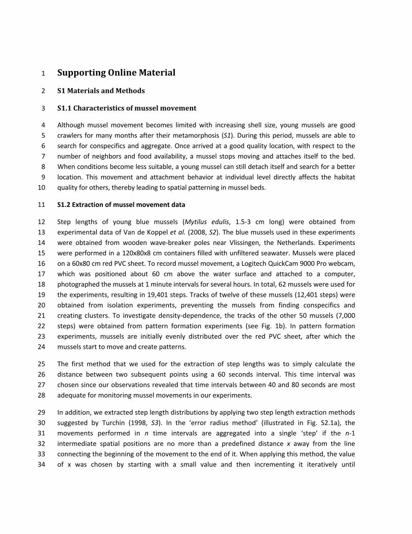
Although mussel movement becomes limited with increasing shell size, young mussels are good 4 crawlers for many months after their metamorphosis (S1). During this period, mussels are able to 5 search for conspecifics and aggregate. Once arrived at a good quality location, with respect to the 6 number of neighbors and food availability, a mussel stops moving and attaches itself to the bed. 7 When conditions become less suitable, a young mussel can still detach itself and search for a better 8 location. This movement and attachment behavior at individual level directly affects the habitat 9 quality for others, thereby leading to spatial patterning in mussel beds. 10
S1.2 Extraction of mussel movement data 11
Step lengths of young blue mussels (Mytilus edulis, 1.5‐3 cm long) were obtained from 12 experimental data of Van de Koppel et al. (2008, S2). The blue mussels used in these experiments 13 were obtained from wooden wave‐breaker poles near Vlissingen, the Netherlands. Experiments 14 were performed in a 120x80x8 cm containers filled with unfiltered seawater. Mussels were placed 15 on a 60x80 cm red PVC sheet. To record mussel movement, a Logitech QuickCam 9000 Pro webcam, 16 which was positioned about 60 cm above the water surface and attached to a computer, 17 photographed the mussels at 1 minute intervals for several hours. In total, 62 mussels were used for 18 the experiments, resulting in 19,401 steps. Tracks of twelve of these mussels (12,401 steps) were 19 obtained from isolation experiments, preventing the mussels from finding conspecifics and 20 creating clusters. To investigate density‐dependence, the tracks of the other 50 mussels (7,000 21 steps) were obtained from pattern formation experiments (see Fig. 1b). In pattern formation 22 experiments, mussels are initially evenly distributed over the red PVC sheet, after which the 23 mussels start to move and create patterns. 24
The first method that we used for the extraction of step lengths was to simply calculate the 25 distance between two subsequent points using a 60 seconds interval. This time interval was 26 chosen since our observations revealed that time intervals between 40 and 80 seconds are most 27 adequate for monitoring mussel movements in our experiments. 28
In addition, we extracted step length distributions by applying two step length extraction methods 29 suggested by Turchin (1998, S3). In the ‘error radius method’ (illustrated in Fig. S2.1a), the 30 movements performed in n time intervals are aggregated into a single ‘step’ if the n‐1 31 intermediate spatial positions are no more than a predefined distance x away from the line 32 connecting the beginning of the movement to the end of it. When applying this method, the value 33 of x was chosen by starting with a small value and then incrementing it iteratively until 34

oversampling was minimized, i.e., until autocorrelation in the turning angle vanished. 35 Autocorrelation was calculated with the acf function in R (R version 2.10.0 © 2009 The R 36 Foundation for Statistical Computing). When the autocorrelation of n data points exceeded the 37 confidence interval derived with the acf function, the distance x was increased by 0.01 cm. 38
Turchin’s ‘angle method’ (illustrated in Fig. S2.1b) concerns the angle between movements. The 39 movements performed in n time intervals are aggregated into a single step if the angle between 40 the starting position and the end position is smaller than a predefined value βmax.. When this value 41 is exceeded after the nth movement, the corresponding point becomes the starting point for the 42 next step. The threshold value βmax was also chosen iteratively, starting with a small angle and 43 gradually increasing it until the autocorrelation in turning angles vanished. 44
As shown in Table S3.1, the method used for estimating step lengths does not affect our 45 conclusions: in all cases, the data are best explained by a Lévy walk, where the pure Lévy walk 46 model performs almost as well as a truncated Lévy walk. In all cases, R2–values of the best‐fitting 47 models exceed 0.995. 48
S1.3 Fitting movement types to step length data 49
The step length data of the mussel movements were used to create a step length frequency 50 distribution (Fig. 1a). When plotted on a log‐log scale, a power‐law probability distribution 51
results in a straight line with slope – . However, drawing conclusions from this kind 52 of presentation can be deceptive (S4‐S6). We therefore used a more robust method (S5) and first 53 determined the inverse cumulative frequency distribution of our data, which for each step length 54 gives the fraction of steps with lengths larger or equal to . This cumulative distribution is plotted 55 in Fig. 1b on a log‐log scale. We compared this distribution with the cumulative probability 56 distribution of three random movement strategies: Brownian walk, Lévy walk, and truncated Lévy 57 walk. 58
Brownian walk 59
Brownian walk is a random movement strategy that corresponds to normal diffusion. The step 60 length distribution can be derived from an exponential distribution with λ > 0: 61
. (1) 62
Lévy walk 63
The frequency distribution of step lengths that characterizes a Lévy walk has a heavy tail and is 64 scale‐free, i.e. the characteristic exponent of the distribution is independent of scale. To fit a Lévy 65 walk to the data, a Pareto distribution (S7) was used: 66
. (2) 67

The shape parameter (which has to exceed 1) is known as the Lévy exponent or scaling exponent 68 and determines the movement strategy (see Fig. S2.2). When is close to 1, the resulting 69 movement strategy resembles ballistic, straight‐line motion, as the probability to move a very 70 large distance is equal to the chance of making a small displacement. A movement strategy is 71 called a Lévy walk when the scaling exponent is between 1 and 3. When μ approaches 1, the 72 movement is approximately ballistic, while it is approximately Brownian when μ approaches 3 73 (and for μ > 3). The Lévy walks found in nature typically have an exponent μ of approximately 2 74 (S4, S8‐S10). is a normalization constant ensuring that the distribution has a total mass 75
equal to 1, i.e. that all values of sum up to 1. If we impose the additional criterion that steps 76 must have a minimum length 0 , this constant is given by 77
1 . (3) 78
When fitting our data to a Lévy walk, we used the value of that provided the best fit of the 79 step length distributions to the actual data. 80
Truncated Lévy walk 81
A truncated Lévy walk differs from a standard Lévy walk in the tail section of the frequency 82 distribution; a truncated Lévy walk has a maximum step size and, as a consequence, loses its 83 infinite variance and scale‐free character at large step sizes. The truncated Lévy walk was 84 represented by the truncated Pareto distribution, which can be described by the same function 85
as a standard Pareto distribution, but with different constant : 86
. (4) 87
In a truncated Lévy walk, step lengths are constrained to the interval . When 88 fitting our data to a truncated Lévy walk, we used those values of and that yielded the 89 best fit of the movement models to the data ( = 0.42 cm and = 58.84 cm). 90
Goodness‐of‐fit and model selection 91
For the frequency distributions mentioned above, the fit to the step length data of solitary mussels 92 was calculated using Maximum Likelihood estimation by fitting the inverse cumulative frequency 93 distribution to that of the experimental data. By comparing the inverse cumulative distributions to 94 that of the data, Goodness‐of‐fit (G) and the Akaike Information Criterion (AIC) were calculated as 95 well as the variance explained by the fitted model (R2). The Goodness‐of‐fit method measures how 96 well the experimental data follows the frequency distributions of the movement strategies; the fit 97 is best when the G‐value is closest to zero. The Goodness‐of‐fit value is calculated as 98
2 ∑ ln , (5) 99

where O is the inverse cumulative distribution of the experimental data and E is that of the fitted 100 movement strategies. We used the inverse cumulative distribution as this is the most robust 101 method to compare the observed and expected distributions (S5). The highest AIC weight, which is 102 calculated by comparing the AIC values, and the highest R2 correspond to the movement type best 103 fitting the actual data (S11). This method was used for the analysis of the movement strategies of 104 the 12 solitary mussels, both individually and as a whole, using the step lengths obtained per 105 minute as well as those derived with the two methods of Turchin (see Fig. S2.1). Additionally, step 106 lengths obtained from pattern formation experiments were grouped for different combinations of 107 local density (within a radius of 3.3 cm) and long‐range density (within a radius of 22.5 cm). These 108 groups of step lengths were used for determining the Lévy exponent at different densities, in 109 order to observe whether a composite Brownian walk exists in mussel movement (see Table S3.2). 110
S1.4 Computer Simulations 111
Individual based model 112
We developed an individual based model that describes pattern formation in mussels by relating 113 the chance of movement to the short‐ and long‐range densities of mussels, following Van de 114 Koppel et al. (2008, S2). Whereas they modeled pattern formation in mussel beds by adjusting the 115 movement speed to the short‐ and long‐range densities (S2), we extracted the stop and move 116 behavior of the mussels from the experimental data. In our model, 2500 ‘mussels’ (with a radius of 117 1.5 cm each) are initially spread homogeneously within a 150 cm by 150 cm arena. Each time step, 118 the short‐range (D1) and long‐range (D2) densities are determined for each individual, based on 119 mussel densities within a radius of 3.3 cm and 22.5 cm, respectively. These radii correspond to the 120 ranges in which we found significant correlations with the probability of moving in a multi‐variate 121 regression analysis of our experimental data (F = 77.17, p << 0.001, R2 = 0.622, df = 136). The 122 probability that a mussel moves is negatively related to the short‐range density D1 and 123 positively related to the long‐range density D2 (see Fig. S2.3), which causes mussels to stay in 124 places where they can aggregate with direct neighbors, but move away from crowded locations 125 where food becomes limiting. In the model, we used a linear relationship between and the 126 two densities: 127
, (6) 128
which was obtained by applying linear regression to our experimental data (a = 0.63, b = 1.26, and 129 c = 1.05). If a mussel decided to move in our model, its step length l was chosen at random from a 130 power law distribution (S12) with a given Lévy exponent μ > 1: 131
1 , (7) 132
where x is a random variable that is uniformly distributed over the unit interval (0 ≤ x ≤ 1), and 133 is the minimum distance traveled when moving (S7), which we have set at 0.3 cm. Each 134

simulation step, mussels move instantaneously from one location to another, though step lengths 135 were truncated when a movement path was obstructed by another mussel. This truncation was 136 calculated by determining the free movement path until collision, using a band width of 3 cm (the 137 size of a mussel) around the line segment connecting the mussels’ original location to its intended 138 destination. When a conspecific was located within this band, the mussel stopped in front of this 139 conspecific, thereby truncating its movement path. All movements occurred simultaneously and 140 all individuals in a simulation used the same movement strategy. 141
As differences occur in the average distance covered per simulation step between the movement 142 strategies (ballistic individuals move a larger distance per simulation step than Lévy or Brownian 143 walkers) and assuming that movement speed is constant, more time is needed for a ballistic step 144 than for a Brownian step. To avoid having Brownian movers switch more frequently between 145 moving and stopping than ballistic movers, we updated the state of either moving or stopping not 146 after each simulation step but after an average distance moved. 147
A simulation was finished when the average short‐range density exceeded 1.5 times the mean 148 long‐range density. At that moment, the total distance travelled was recorded. As we assume that 149 the movement speed is constant, the rate of patterning is proportional to the normalized inverse 150 of the distance traversed until a pattern is formed. Simulations were run for a range of Lévy 151 exponents (1 < μ ≤ 3), and for each value the rate of pattern formation was plotted as a function of 152 μ. The model was implemented in Matlab version 7.9 (©1984‐2009. The MathWorks, Inc.). 153
Evolutionary model 154
Evolutionary change was studied in a monomorphic resident population by investigating whether 155 the fitness of rare mutants is higher than that of the residents, implying that the mutants can 156 increase in frequency (S13, S14). After the mussels moved an equal distance, we recorded the 157 short‐range density, the long‐range density, and the fraction of mussels that was still moving, for 158 both the residents and the mutants. In a population with non‐overlapping generations, fitness is 159 given by the product of survival probability and fecundity. We assumed that survival probability is 160 proportional to the local mussel density D1 and that fecundity is inversely proportional to the long‐161 range density D2 (as this density affects food supply) and to the time X spent on moving (as energy 162 spent on moving cannot be invested in offspring production). Dividing the fitness measures thus 163 obtained for a mutant and a resident results in a measure for the relative fitness of the mutant 164 strategy: 165
,
, ,
, . (8) 166
Mutant strategies with a relative fitness value larger than one will invade and potentially take over 167 the resident population. For any combination of resident and mutant movement strategy, the 168 relative fitness of the mutants is depicted in a pairwise invasibility plot (S14, see Fig. 3). In this plot, 169

the color red indicates that the mutant has a higher fitness than the resident (Fmut > 1), while the 170 color green indicates that the mutant cannot invade the resident population (Fmut < 1). The 171 intersection of the line separating these two scenarios (Fmut = 1) with the main diagonal of the 172 pairwise invasibility plot corresponds to an evolutionarily singular strategy (S13, S14). 173

S2 Supporting Online Figures
Fig. S2.1. Step length calculation using the ‘error radius method’ (A) and the ‘angle method’ (B). In the first method (A), n steps are aggregated into one move if the n‐1 intermediate spatial positions are no more than x units away from the line connecting the beginning of the step to the end of it. The second method (B) is based on reorientation events; when the angle β (between the dotted black line and the solid black line) exceeds a certain threshold value, the corresponding point is the next new point (after Turchin, 1998; S3).

Fig. S2.2. The Lévy exponent μ determines the shape of the step length distribution and thus the movement strategy. When μ is close to 1, the movement strategy resembles ballistic, straight‐line motion (A, D), whereas the step length distribution is similar to that of a Brownian walk when μ approaches 3 (C, F). The movement strategy is referred to as a Lévy walk when 1 < μ < 3 (B, E). A, B, and C show movement trajectories obtained with μ = 1.01, 2, and 3, respectively. The inverse cumulative step length frequency distributions (i.e. the fraction of steps that is larger than or equal to the displacement length (l) that is given on the x‐axis) are given by D, E, and F for μ = 1.01, 2, and 3, respectively.

Fig. S2.3. Experimental data shows that the probability of moving depends on short‐range and long‐range mussel densities. (A) Local mussel density decreases the probability of moving; mussels tend to stay in denser clumps. (B) The probability of moving positively correlates with long‐range density; mussels move away from areas where competition is high.

S3 Supporting Online Tables
Table S3.1. Summary of the model fits to the step length data. Goodness‐of‐fit (G), AIC weights and % variance explained of each movement strategy fitted to the mussel data (R2) for all three methods that were used to obtain the step lengths. Truncated Lévy walk (TLW) corresponds best to the raw data and the data obtained using the error radius method. Data acquired with the angle method was best described by a Lévy walk (LW). Lévy exponents ranged from 1.930 to 2.174, with a mean μ of 2.032.
Method Model G AIC weights Adjusted R2 Lévy exponent
Step per minute
Truncated Lévy walk 33.60 0.446 0.999 2.127
Lévy walk 64.54 0.431 0.999 2.174
Brownian walk ‐119.43 0.123 0.878 ‐
Error radius method
Truncated Lévy walk ‐2.69 0.437 0.997 1.967
Lévy walk 3.93 0.401 0.995 2.045
Brownian walk ‐344.85 0.163 0.898 ‐
Angle method Truncated Lévy walk 36.43 0.445 0.995 1.930
Lévy walk 73.20 0.453 0.996 1.946
Brownian walk ‐106.00 0.103 0.734 ‐

Table S3.2. Lévy exponent during pattern formation. Lévy exponents for step lengths in different local and long‐range density groups, for all three methods that were used to obtain the step lengths. Low/Low = both low local and long‐range densities; Low/High = low local and high long‐range density; High/Low = high local and low long‐range density; High/High = both high local and long‐range densities. Pattern formation in mussel beds produces an environment with high local densities and low long‐range densities. There is no significant correlation between Lévy exponent and the degree of patterning, as well as any other relationship between the exponent and mussel density; we can therefore reject the hypothesis of a composite Brownian walk, where movement speeds are adjusted to local environmental conditions (S15‐S18).
Method Low/Low Low/High High/Low High/High
Step per minute 2.05 2.05 2.06 2.05
Error radius method
2.00 2.07 2.05 2.05
Angle method 2.00 2.00 2.00 2.00

S4 Supporting Online References
S1. R. A. Maas Geesteranus, Arch Neerl Zool 6, 283 (1942). S2. J. van de Koppel et al., Science 322, 739 (2008). S3. P. Turchin, Quantitative Analysis of Movement. (Sinauer Associates, 1998). S4. D. W. Sims, D. Righton, J. W. Pitchford, J. Anim. Ecol. 76, 222 (2007). S5. A. M. Edwards et al., Nature 449, 1044 (2007). S6. E. P. White, Ecology 89, 2971 (2008). S7. A. Clauset, C. R. Shalizi, M. E. J. Newman, SIAM Rev. 51, 661 (2009). 10. G. Ramos‐Fernandez et al., Behav. Ecol. Sociobiol. 55, 223 (2004). 11. A. M. Reynolds et al., Ecology 88, 1955 (2007). 12. N. E. Humphries et al., Nature 465, 1066 (2010). S11. K. P. Burnham, D. R. Anderson, Model selection and multimodel inference: A practical information‐theoretic
approach (Springer‐Verlag, 2002). S12. M.E.J. Newman, Contemp. Phys. 46, 323 (2005). S13. S. A. H. Geritz, E. Kisdi, G. Meszena, J. A. J. Metz, Evol. Ecol. 12, 35 (1998). S14. F. Dercole, S. Rinaldi, Analysis of evolutionary processes: the adaptive dynamics approach and its applications
(Princeton University Press, 2008) S15. S. Benhamou, Ecology 88, 1962 (2007). S16. A. Reynolds, Ecology 89, 2347 (2008). S17. S. Benhamou, Ecology 89, 2351 (2008). S18. B. A. Nolet, W. M. Mooij, J. Anim. Ecol. 71, 451 (2002).
Movie S1
1201187S1.mov: Time‐laps movie showing the movement behavior of a single mussel, with the corresponding movement track plotted as the mussel is moving. The video covers nearly a two hour time period (QuickTime movie, 11 MB), with images taken every 10 seconds. We acknowledge Aniek van den Berg for running this movement experiment.
Matlab code:
IBM1201187S1.m: Individual Based model of mussels moving into a self‐organized pattern. The code was written for Matlab version 7.9.0 (R2009b © The Mathworks, Inc.) and shows the distribution of mussels after each simulation step.

Comment on “Lévy Walks EvolveThrough Interaction Between Movementand Environmental Complexity”Vincent A. A. Jansen,1* Alla Mashanova,1 Sergei Petrovskii2
de Jager et al. (Reports, 24 June 2011, p. 1551) concluded that mussels Lévy walk. We confronteda larger model set with these data and found that mussels do not Lévy walk: Their movement isbest described by a composite Brownian walk. This shows how model selection based on animpoverished set of candidate models can lead to incorrect inferences.
ALévy walk is a form of movement inwhich small steps are interspersed withvery long ones, in such a manner that
the step length distribution follows a power law.Movement characterized by a Lévy walk has nocharacteristic scale, and dispersal is superdiffu-sive so that individuals can cover distance muchquicker than in standard diffusion models. de Jageret al. (1) studied the movements of individualmussels and concluded that mussels moveaccording to a Lévy walk.
The argument of (1) is based on model se-lection, a statistical methodology that comparesa number of models—in this case, different steplength distributions—and selects the model thatdescribes the data best as themost likelymodel toexplain the data (2). This methodology is used toinfer types of movements of animals (3) and hasled to a number of studies that claim Lévy walksare often encountered in the movement of ani-mals. The methodology in (1) contrasts a power-law distribution, which is indicative of a Lévywalk, with an exponential distribution, whichindicates a simple random walk. If one has tochoose between these alternatives, the power-lawdistribution gives the best description. However,if a wider set of alternatives is considered, thisconclusion does not follow.
Heterogeneity in individual movement be-havior can create the impression of a power law(4–6). Mussels’ movement is heterogeneous asthey switch between moving very little or not atall, and moving much farther (1, 7). If musselsswitch between differentmodes, and in eachmodedisplay Brownianmotion, this suggests the use ofa composite Brownian walk, which describes themovement as a sum of weighted exponential dis-tributions. We confronted this plausible modelwith the mussel movement data (8).
Visual inspection of the data shows that thecumulative distributionof step lengths has a humped
pattern that is indicative of a sum of exponentials(Fig. 1A). We applied a model selection pro-cedure based on the Akaike information criterion(AIC) (2, 3). We compared six different steplength distributions: an exponential distribution,
a power law, a truncated power law, and threehyperexponential distributions (a sum of two,three, or four exponentials to describe compositeBrownian walks). We did this for the data trun-cated as in (1) (Fig. 1A) as well as all the full,untruncated data set (Fig. 1B). In both cases, wefound that the composite Brownian walk con-sisting of the sum of three exponentials was thebest model (Fig. 1 and Table 1). This convinc-ingly shows that the mussels described in (1) donot do a Lévy walk. Only when we did not takethe composite Brownian walk models intoaccount did the truncated power law modelperform best and could we reproduce the resultin (1).
Mussel movement is best described by acomposite Brownian walk with three modes ofmovement with different characteristic scales be-tween which the mussels switch. The mean move-ment in these modes is robust to truncation of thedata set, in contrast to the parameters of the powerlaw, which were sensitive to truncation [Table 1;
TECHNICALCOMMENT
1School of Biological Sciences, Royal Holloway, University ofLondon, Surrey TW20 0EX, UK. 2Department of Mathematics,University of Leicester, Leicester LE1 7RH, UK.
*To whom correspondence should be addressed. E-mail:[email protected]
Fig. 1. The step lengthdistribution for musselmovement [as in (10)]and curves depicting someof the models. The circlesrepresent the inverse cu-mulative frequency of steplengths, The curves repre-sent Brownian motion(blue), a truncated powerlaw (red), and a compositeBrownian walk consistingof a mixture of three ex-ponentials (blue-green). (A)Data as truncated in Fig.1 in (1, 10) (2029 steps).(B) The full untruncateddata set (3584 steps).
24 FEBRUARY 2012 VOL 335 SCIENCE www.sciencemag.org918-c
on
Feb
ruar
y 24
, 201
2w
ww
.sci
ence
mag
.org
Dow
nloa
ded
from

also see supporting online material (SOM)]. Thisanalysis does not tell us what thesemodes are, butwe speculate that it relates to the stop-movebehavior that mussels show, even in homoge-neous environments (1). We speculate that themode with the smallest average movement(~0.4 mm) is related to nonmovement, combinedwith observational error. The next mode (averagemovement ~1.5 mm) is related to mussels movingtheir shells but not displacing, and the mode withthe largestmovements (on average 14mm, about thesize of a small mussel) is related to actual dis-placement. This suggests that in a homogeneousenvironment, mussels are mostly stationary, andif they move, they either wobble or move aboutrandomly. Indeed, if we removemovements smallerthan half the size of a small mussel (7.5 mm), theremaining data points are best described byBrownian motion. This shows that mussel move-ment is not scale invariant and not superdiffusive.
de Jager et al.’s analysis (1) does show thatmussels do not perform a simple random walkand that they intersperse relatively long displace-ments with virtually no displacement. However,one should not infer from that analysis that themovement distribution therefore follows a powerlaw or that mussels move according to a Lévywalk, and there is no need to suggest that mussels
must possess some form of memory to produce apower law–like distribution (9). Having includedthe option of a composite Brownian walk, whichwas discussed in (1) but not included in the set ofmodels tested, one finds that this describesmussels’ movement extremely well.
Our analysis illustrates why one has to becautious with inferring that animalsmove accord-ing to a Lévy walk based on too narrow a set ofcandidate models: If one has to choose between apower law and Brownian motion, often the powerlaw is best, but this could simply reflect theabsence of a better model. To make defensibleinferences about animal movement, model selec-tion should start with a set of carefully chosenmodels based on biologically relevant alterna-tives (2). Heterogeneous random movement oftenprovides such an alternative and has the addition-al advantage that it can suggest a simple mech-anism for the observed behavior.
References and Notes1. M. de Jager, F. J. Weissing, P. M. J. Herman, B. A. Nolet,
J. van de Koppel, Science 332, 1551 (2011).2. K. P. Burnham, D. R. Anderson, Model Selection and
Multimodel Inference: A Practical Information-TheoreticApproach (Springer-Verlag, New York, ed. 2, 2002).
3. A. M. Edwards et al., Nature 449, 1044 (2007).4. S. Benhamou, Ecology 88, 1962 (2007).
5. S. V. Petrovskii, A. Y. Morozov, Am. Nat. 173, 278(2009).
6. S. Petrovskii, A. Mashanova, V. A. A. Jansen, Proc. Natl.Acad. Sci. U.S.A. 108, 8704 (2011).
7. J. van de Koppel et al., Science 322, 739 (2008).8. We found that the results published in (1) were
based on a corrupted data set and that there wereerrors in the statistical analysis. [For details, see ourSOM and the correction to the de Jager paper (10).]Here, we analyzed a corrected and untruncated dataset provided to us by M. de Jager on 20 October 2011.This data set has 3584 data points, of which 2029remain after truncation. Since doing our analysis, anamended figure has been published (10), whichappears to be based on ~7000 data pointsafter truncation.
9. D. Grünbaum, Science 332, 1514 (2011).10. M. de Jager, F. J. Weissing, P. M. J. Herman, B. A. Nolet,
J. van de Koppel Science 334, 1641 (2011).
Acknowledgments: We thank M. de Jager for supplyingthe data to do this analysis and the authors of (1) fortheir constructive comments. This work was funded byBiotechnology and Biological Sciences Research CouncilGrant BB/G007934/1 (to V.A.A.J.) and Leverhulme TrustGrant F/00 568/X (to S.P.).
Supporting Online Materialwww.sciencemag.org/cgi/content/full/335/6071/918-c/DC1Materials and MethodsSOM TextReferences
25 October 2011; accepted 13 January 201210.1126/science.1215747
Table 1. ModelparametersandAkaikeweights. Themaximumlikelihoodparameterestimates, log maximum likelihoods (ML), AIC values, and Akaike weights arecalculated (for details, see SOM) for the data shown in Fig. 1, A and B. The Akaikeweights without the composite Brownianwalks are given in brackets.We analyzed the
full data set (*) with xmin=0.02236mm, and the data set truncated as in (1) (†) withxmin = 0.21095 mm. For xmax, the longest observed step length (103.9mm) wasused. The mix of four exponentials is not the best model according to the AICweights. It gives a marginally, but not significantly, better fit and is overfitted.
Models Formula Parameters* Parameters† ML AIC Weight
Exponential(Brownianmotion)
P(X = x) = le −l(x− xmin) l = 1.133 l = 0.770 –3136.89*–2558.67†
6275.78*5119.37†
0 (0)*0 (0)†
Power law(Lévy walk)
P(X = x) = m−1x1 − mmin
x−m m = 1.397 m = 1.975 –2290.10*–1002.32†
4582.20*2006.64†
0 (0) *0 (0.006)†
Truncatedpower law(Lévy walk)
P(X = x) = m−1x1 − mmin − x1 − m
maxx−m m = 1.320 m = 1.960 –2119.55*
–997.29†4241.10*1996.58†
0 (1) *0 (0.994)†
Mix of twoexponentials(CompositeBrownian walk)
P(X = x) =X
i=1
2
pilie−li(x − xmin)
withX
i=1
2
pi = 1
p = 0.073,l1 = 0.122,l2 = 3.238
p = 0.127,l1 = 0.123,l2 = 3.275
–906.15*–1022.44†
1818.31*2050.87†
0*0†
Mix of threeexponentials(CompositeBrownian walk)
P(X = x) =X
i=1
3
pilie−li(x − xmin)
withX
i=1
3
pi = 1
p1 = 0.034,p2 = 0.099,l1 = 0.069,l2 = 0.652,l3 = 3.613
p1 = 0.063,p2 = 0.210,l1 = 0.072,l2 = 0.832,l3 = 4.309
–861.55*–966.70†
1733.11*1943.40†
0.881*0.873†
Mix of fourexponentials(CompositeBrownian walk)
P(X = x) =X
i=1
4
pilie−li(x − xmin)
withX
i=1
4
pi = 1
p1 = 0.014,p2 =0.034,p3 = 0.085,l1 = 0.656,l2 = 0.069,l3 = 0.652l4 = 3.613
p1 = 0.017,p2 = 0.060,p3 = 0.202,l1 = 0.377,l2 = 0.070,l3 = 0.902,l4 = 4.345
–861.55*–966.63†
1737.11*1947.26†
0.119*0.127†
www.sciencemag.org SCIENCE VOL 335 24 FEBRUARY 2012 918-c
TECHNICAL COMMENT
on
Feb
ruar
y 24
, 201
2w
ww
.sci
ence
mag
.org
Dow
nloa
ded
from

Response to Comment on “Lévy WalksEvolve Through Interaction BetweenMovement and Environmental Complexity”Monique de Jager,1* Franz J. Weissing,2 Peter M. J. Herman,1
Bart A. Nolet,3,4 Johan van de Koppel1,2,4
We agree with Jansen et al. that a composite movement model provides a better statisticaldescription of mussel movement than any simple movement strategy. This does not underminethe take-home message of our paper, which addresses the feedback between individualmovement patterns and spatial complexity. Simple movement strategies provide more insightin the eco-evolutionary analysis and are therefore our model of choice.
The purpose of our paper (1, 2) was todemonstrate that movement strategies areshaped by the interaction between individ-
ual selection and the formation of spatial com-plexity on the population level. We showed thatin a family of movement models ranging fromballistic motion, to Lévy walk, to Brownian mo-tion, a Lévy walk with exponent m ≈ 2 is theoptimal strategy for mussels involved inpattern formation. Within this family of models,a single parameter (the scaling exponent m)distinguishes between the different movementstrategies. We intentionally chose a one-dimensionalstrategy space that can easily be used in pairwiseinvasibility analyses and the subsequent pair-
wise invasibility plots. It also keeps focus on themain differences in movement strategy, contrast-ing ballistic movement, Brownian diffusion, andlong-tailed step length distributions, as in Lévywalks. As is often the case, the better fit of thecomplex model (i.e., composite Brownian walk)trades off with the elegance and clarity of thesimpler model.
Nevertheless, it might be interesting to ex-amine the mechanisms behind the compositeBrownian walk that was observed in our musselmovement data by Jansen et al. (3). Below, weinvestigate three possible causes of the observedmovement pattern: (i) mussels switch betweenmultiple movement modes because of changesin environmental conditions; (ii) the (collective)composite Brownian walk might be an ensem-ble of different individual Brownian walks; or(iii) internal switches between movement modesexist, with which mussels try to approximate aLévy walk.
The first possible mechanism behind a com-posite Brownian walk is that mussels switch be-tween movement modes in response to changesin environmental conditions. For example, acomposite Brownian walk will result if animals
switch between local Brownian search within aresource patch and straight-lined ballistic searchbetween patches (4–6). Because the solitary mus-sels in our experiment were situated in a bare,homogeneous environment, repeated switchesbetween movement strategies induced by chang-ing environmental conditions do not provide aplausible explanation for the observed compos-ite walk.
A second possible explanation for the ob-served composite Brownian walk could bethat variation in individual movement behaviorcan explain the improved fit by the compositeBrownian model (7)—for example, multiple dif-ferent Brownian walks together make up theobserved composite walk. To investigate this,we examined the individual movement tracksof the 12 mussels in our experiment. We indeedfound a large variety of movement trajectories(Fig. 1); some mussels moved a large distance,whereas others stayed approximately at theoriginal location. We fitted a Brownian walk,a Lévy walk, a truncated Lévy walk, and twocomposite Brownian walks to these individualmovement trajectories, using the corrected dataset and the analysis suggested by Jansen et al.(2, 3). The analysis (Table 1 and Fig. 2) revealsthat, in most cases, a Brownian walk fitted verypoorly to the data. A truncated Lévy walk pro-vided large improvement over a Brownian walk,whereas a composite Brownian walk providedonly small further improvement in fit, indicatingthat even at the individual level, compositebehavior might underlie a long-tailed movementpattern.
A third possibility to mechanistically under-pin the improved fit by a composite Brownianwalk is that mussels use an internal switching ruleto alternate between movement modes, indepen-dent from external triggers. Our study (1, 2)shows that a long-tailed step length distributionis a rewarding strategy for mussels living in, andcontributing to, a spatially complex system. It isnot obvious, however, how an animal shouldachieve such a step length distribution in prac-
TECHNICALCOMMENT
1Spatial Ecology Department, Royal Netherlands Institute forSea Research (NIOZ), Post Office Box 140, 4400 AC Yerseke,Netherlands. 2Theoretical Biology Group, Centre for Ecologicaland Evolutionary Studies, University of Groningen, Nijenborgh7, 9747 AG Groningen, Netherlands. 3Department of AnimalEcology, Netherlands Institute of Ecology (NIOO-KNAW), PostOffice Box 50, 6700 AB Wageningen, Netherlands. 4ProjectGroup Movement Ecology, Netherlands Institute of Ecology(NIOO-KNAW), Post Office Box 50, 6700 AB Wageningen,Netherlands.
*To whom correspondence should be addressed. E-mail:[email protected]
Fig. 1. Movement trajec-tories of the 12 mussels onwhich we based the modelfitting in (1, 4).
24 FEBRUARY 2012 VOL 335 SCIENCE www.sciencemag.org918-d
on
Feb
ruar
y 24
, 201
2w
ww
.sci
ence
mag
.org
Dow
nloa
ded
from

tice. It is possible that animals approximate aLévy walk by adopting an intrinsic compos-ite movement strategy with different modes(which do not necessarily need to be Brown-ian). The observation by Jansen et al. (3) thata composite walk yields a better fit to the ob-servations thus suggests an interesting solu-tion for this problem, which is worth furtherinvestigation. However, we think it most ad-visable to examine this switching behavior bymeans of temporal and spatial correlations ofmovement steps within animal tracks ratherthan fitting multimodal models to step sizedistributions. In our opinion, the observation byJansen et al. (3) does not change the overall con-clusion of our paper (1), but it may contribute toa better understanding of the behavioral mech-anisms by which animals achieve their optimalmovement strategy.
References and Notes1. M. de Jager, F. J. Weissing, P. M. J. Herman, B. A. Nolet,
J. van de Koppel, Science 332, 1551 (2011).2. M. de Jager, F. J. Weissing, P. M. J. Herman, B. A. Nolet,
J. van de Koppel, Science 334, 1641 (2012).3. V. A. A. Jansen, A. Mashanova, S. Petrovskii, Science 335,
918 (2012); www.sciencemag.org/cgi/content/full/335/6071/918-c.
4. M. J. Plank, A. James, J. R. Soc. Interface 5, 1077(2008).
5. S. Benhamou, Ecology 88, 1962 (2007).6. A. M. Reynolds, Physica A 388, 561 (2009).7. S. Petrovskii, A. Mashanova, V. A. A. Jansen, Proc. Natl.
Acad. Sci. U.S.A. 108, 8704 (2011).8. K. P. Burnham, D. R. Anderson, Model Selection and
Multimodal Inference: A Practical Information-TheoreticApproach (Springer-Verlag, New York, ed. 2, 2002).
Acknowledgments: We thank A. Edwards, F. van Langevelde,and V. Jansen et al. for their comments and suggestions.The authors declare no competing financial interests. Theresearch of M.d.J. is supported by a grant from the NetherlandsOrganization of Scientific Research/Earth and Life Sciences(NWO-ALW). This is publication 5183 of the NetherlandsInstitute of Ecology (NIOO-KNAW).
18 November 2011; accepted 13 January 201210.1126/science.1215903
Table 1. Comparison of five movement models (Brownian walk, BW; Lévy walk, LW; truncated Lévywalk, TLW; composite Brownian walk with two movement modes, CBW2; composite Brownian walkwith three movement modes, CBW3) for the eight mussels for which sufficient data (n > 50) wereavailable. For each mussel, the table presents the Akaike information criterion (AIC) and the Akaikeweights (wAIC) for the five movement models. The minimal AIC value (corresponding to the bestmodel) is shown in bold. The Akaike weights correspond to the relative likelihood of each model(8). For all model fits, we used a lower boundary (lmin) of 0.2 mm.
BW LW TLW CBW2 CBW3Mussel
AIC wAIC AIC wAIC AIC wAIC AIC wAIC AIC wAIC
A 1917.4 0.000 1262.7 0.000 1236.6 0.000 1192.4 0.006 1182.12 0.994B 1293.2 0.867 2030.8 0.000 1618.1 0.000 1297.2 0.117 1301.2 0.016D 330.4 0.000 282.5 0.000 256.1 0.000 209.1 0.502 209.2 0.498F 1101.7 0.000 642.3 0.000 628.9 0.054 638.8 0.000 623.2 0.945G 1410.7 0.000 792.4 0.000 770.8 0.000 761.6 0.001 748.5 0.998H 625.5 0.000 775.6 0.000 750.3 0.000 519.9 0.881 523.9 0.119I 2177.2 0.000 1650.0 0.000 1592.5 0.003 1582.1 0.620 1583.1 0.376L 1455.8 0.000 1179.0 0.000 1129.0 0.002 1123.2 0.033 1116.4 0.966
Fig. 2. Inverse cumula-tive frequency distribution(e.g., the fraction of steplengths that is larger thanor equal to a given steplength) of the movementpatterns of 12 individualmussels (thin dashed anddotted lines) and the com-bined data set (thick lineand large dots).
www.sciencemag.org SCIENCE VOL 335 24 FEBRUARY 2012 918-d
TECHNICAL COMMENT
on
Feb
ruar
y 24
, 201
2w
ww
.sci
ence
mag
.org
Dow
nloa
ded
from