Thilo A. Schmitt, Rudi Schäfer, Holger Dette, Thomas … · SFB 823 Quantile correlations: Uncovering temporal dependencies in financial time series Discussion Paper Thilo A. Schmitt,

SFB 823

Quantile correlations: Uncovering temporal dependencies in financial time series

Discussion P

aper

Thilo A. Schmitt, Rudi Schäfer, Holger Dette, Thomas Guhr

Nr. 28/2014

August 5, 2014 12:56 WSPC/INSTRUCTION FILE rank

Quantile correlations: Uncovering temporal dependencies in financial

time series

THILO A. SCHMITT

Fakultat fur Physik, Universitat Duisburg-Essen, Lotharstr. 147048 Duisburg, Germany

[email protected]

RUDI SCHAFER

Fakultat fur Physik, Universitat Duisburg-Essen, Lotharstr. 1

47048 Duisburg, Germany

HOLGER DETTE

Fakultat fur Mathematik, Ruhr-Universitat Bochum

44780 Bochum, Germany

THOMAS GUHR

Fakultat fur Physik, Universitat Duisburg-Essen, Lotharstr. 1

47048 Duisburg, Germany

We conduct an empirical study using the quantile-based correlation function to uncoverthe temporal dependencies in financial time series. The study uses intraday data forthe S&P 500 stocks from the New York Stock Exchange. After establishing an empiri-

cal overview we compare the quantile-based correlation function to stochastic processesfrom the GARCH family and find striking differences. This motivates us to propose the

quantile-based correlation function as a powerful tool to assess the agreements betweenstochastic processes and empirical data.

1. Introduction

Financial time series exhibit various non-trivial properties. The distribution of re-

turns deviates from a normal distribution and shows heavy tails (Oliver 1926, Mills

1927, Mandelbrot 1963). This behavior was first observed by Mitchell (1915). In

stochastic volatility models the normal distribution is combined with a distribu-

tion for the variances. The resulting return distribution shows non-normality, see

e.g., Clark (1973) and Yang (2004). However, simply drawing volatilities from a

distribution does not account for the empirically observed volatility clustering, i.e.,

temporal inhomogeneity. To achieve this the description by stochastic processes is

essential. In his groundbreaking work Engle made great strides towards this goal

by introducing the ARCH process, see Engle (1982).

The autocorrelation of the return time series is zero (Pagan 1996). However, the

autocorrelation of the time series for absolute or squared returns is non-zero and

1


2

slowly decays to zero for larger lags (Ding et al. 1993, Cizeau et al. 1997, Liu et al.

1997). This effect can be traced back to volatility clustering Mandelbrot (1963).

In high volatility phases the probability that a large (absolute) return is followed

by another large return is higher than normal. The same holds true for phases of

small volatility, where small returns are followed by small returns with higher prob-

ability. Closely related is the so called “leverage effect”. It is empirically known

that volatilities and returns show a negative correlation. This was first observed

by Black (1976) and attributed to the fact that stocks with falling prices are riskier

and therefore have a higher volatility. The reduced market capitalization relative

to the debt of the company makes it more leveraged, hence the name. This ex-

planation is often challenged in the literature (Figlewski and Wang 2000, Aydemir

et al. 2006, Aıt-Sahalia et al. 2013). The studies of these effects typically focuses on

the autocorrelation of return time series or cross correlations between returns and

historical or implied volatilities.

A common tool to analyze temporal dependencies in time series is the L2-

periodogram, which is intrinsically connected to mean values and covariances and

has several optimality properties for the analysis of Gaussian series. On the other

hand it is well known that this periodogram has difficulties to detect nonlinear dy-

namics such as changes in the conditional shape (skewness, kurtosis) or heavy tails,

and several modifications have been proposed to address these problems. Laplace

periodograms have been investigated as an alternative to the ordinary periodogram

by Li (2008, 2012) for analyzing heart rate variability and sun spot data, in the fre-

quency domain. These peridograms are based on quantile regression methodology,

see Koenker (2005) and extensions, which are independent with respect to mono-

tone transformation of the data have been developed by Dette et al. (2011) and

Hagemann (2013). These authors propose a different periodogram, which is defined

as the discrete Fourier transform of quantile-based correlations, see Kedem (1980)

and develop a corresponding statistical theory.

Here, we want to show that even the direct use of quantile-based correlations

provides a very powerful tool to investigate nonlinear dynamics of financial series in

the time domain. For this purpose we conduct an empirical study on intraday data

from stocks in the Standard & Poor’s 500-index (S&P500) during the years 2007

and 2008. In addition, we show that quantile-based correlation is able to uncover

subtle differences between stochastic processes and empirical data. As an example,

we study the return time series from GARCH (Bollerslev 1986), EGARCH (Nelson

1991) and GJR-GARCH (Glosten et al. 1993) processes.

2. Quantile-based correlation

Given a time series x = (x1, x2, . . . , xT ) of length T we calculate the quantile-based

correlation in the following way. Let α ∈ [0, 1] and β ∈ [0, 1] be probability levels.

Then, let qα be the value at the α-quantile for the time series x. We first map the


3

time series x to a filtered time series ξ(α) according to a filter rule

ξ(α)t =

{1 , xt ≤ qα0 , otherwise

. (2.1)

For example, if the time series is

x = (1,−5, 10, 0,−6,−2,−2, 2, 0, 2) (2.2)

we have q0.5 = 0 for the 0.5-quantile and the filtered time series is

ξ(0.5) = (0, 1, 0, 1, 1, 1, 1, 0, 1, 0) . (2.3)

Analogously, we construct a second filtered time series ξ(β) based on a second β-

quantile. We then calculate the lagged cross-correlation of the filtered time series

for each lag l ∈ (−T/2, T/2)

qcf l(ξ(α), ξ(β)) =

1

T

T−l∑t=1

(ξ(α)t − ξ(α))(ξ(β)t+l − ξ(β))

σ(α)σ(β)(2.4)

where ξ(α) denotes the mean value of the filtered time series ξ(α). The standard

deviation of the filtered time series is denoted by σ(α). The basic idea of quantile-

based filtered binary time series was first put forward by Kedem (1980).

The case of equal probability levels in the time domain is discussed in Linton

and Whang (2007) and Hagemann (2013) who proposed a discrete Fourier trans-

form of the correlations in (2.4) with fixed α = β in order to develop robust spectral

analysis. For an alternative estimate and the case α 6= β see Dette et al. (2011).

We calculate 95% confidence intervals for the quantile correlation functions by tak-

ing the standard deviation of the fluctuations of the (0.5, 0.5) quantiles around zero

and multiply them with the standard score of 1.96 corresponding to a 0.95 confi-

dence level. This mitigates problems which would be introduced using the standard

approach for confidence intervals, i.e., 1.96 divided by the square root of the sample

size, which assumes that the elements of the time series are i.i.d. This assumption

is not valid for the financial data we consider in the following.

From the setup of the quantile correlation function we immediately see that

for equal probabilities α = β Eq. (2.4) yields the autocorrelation of the fil-

tered time series. In this case the quantile correlation function is symmetric, i.e.,

qcf l(ξ(α), ξ(α)) = qcf−l(ξ

(α), ξ(α)). If the probabilities differ, α 6= β, the quantile

correlation function is not necessarily symmetric.

We now clarify the meaning of possible combinations for α and β. We denote the

combination of probabilities with (α, β). For example, if we choose the (0.05, 0.05)

quantiles, the filtered time series will each contain 5% ones, which correspond to

the smallest 5% of values in the time series x according to Eq. (2.1). In this case,

we correlate the smallest values of the time series in Eq. (2.4). On the other hand,

consider the (0.95, 0.95) quantiles. Here, we correlate the 95% of the smallest values

of the time series x. However, in the case of financial time series it is more interesting

to know how the largest 5% of values are correlated. The (0.95, 0.95) quantiles also


4

indicate this. We notice that if we change the less-than or equal to sign in Eq. (2.1) to

a greater-than sign for both filtered time series ξ(α) and ξ(β) we get the complement

of the filtered time series, i.e., ones become zeroes and zeroes become ones. Readers

with a background in computer science will notice that this is equivalent to a binary

NOT operation on each filtered time series. As long as this operation is performed

on both filtered time series the sign of the quantile correlation function will not

change, compare Eq. (2.4). This leads us to the interesting case where we want to

know how the smallest 5% values are correlated to the largest 5%. We choose the

(0.05, 0.95) quantiles and effectively correlate the smallest 5% of the values with the

smallest 95%. To answer the question, we have to change the lesser-than or equal to

sign only for the second filtered time series ξ(0.95). This results in a change of sign

for the quantile correlation function. Suppose we find a negative correlation for the

(0.05, 0.95) quantiles. This means that the smallest 5% and 95% of the time series

are negatively correlated. At the same time it implies that the smallest 5% and the

largest 5% of the time series are positively correlated. To keep the notation simple,

we will always calculate the filtered time series according to Eq. (2.1) and mention

how to interpret the quantile correlation function in the given context.

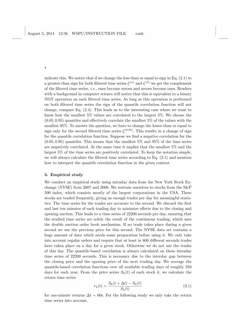
3. Empirical study

We conduct an empirical study using intraday data from the New York Stock Ex-

change (NYSE) from 2007 and 2008. We restrain ourselves to stocks from the S&P

500 index, which consists mostly of the largest corporations in the USA. These

stocks are traded frequently, giving us enough trades per day for meaningful statis-

tics. The time series for the trades are accurate to the second. We discard the first

and last ten minutes of each trading day to minimize effects due to the closing and

opening auction. This leads to a time series of 22200 seconds per day, ensuring that

the studied time series are solely the result of the continuous trading, which uses

the double auction order book mechanism. If no trade takes place during a given

second we use the previous price for this second. The NYSE data set contains a

huge amount of data which needs some preparation before using it. We only take

into account regular orders and require that at least in 800 different seconds trades

have taken place on a day for a given stock. Otherwise we do not use the trades

of this day. The quantile-based correlation is always calculated on these intraday

time series of 22200 seconds. This is necessary due to the interday gap between

the closing price and the opening price of the next trading day. We average the

quantile-based correlation functions over all available trading days of roughly 250

days for each year. From the price series Sk(t) of each stock k, we calculate the

return time series

rk(t) =Sk(t+ ∆t)− Sk(t)

Sk(t)(3.1)

for one-minute returns ∆t = 60s. For the following study we only take the return

time series into account.


5

3.1. Empirical data

We study the quantile-based correlation for six different quantile pairs (α, β). Fig-

ure 1 shows the quantile-based correlation for Abercrombie & Fitch Co. (ANF).

The (0.05, 0.05) quantiles correlate only the largest negative returns, while the

(0.95, 0.95) quantiles indirectly correlate the largest positive returns. This requires

further explanation. In principle, the (0.95, 0.95) quantiles correlate, according to

Eq. (2.1), all returns which are smaller than the 0.95-quantile. This is equivalent

to the statement that the largest 5% of returns are correlated, because if we switch

both lesser signs in Eq. (2.1) to greater signs the quantile correlation function will

not change as discussed in section 2. In both cases the correlation is non-zero and

decays up to lags of roughly one hour to zero.

-0.04

-0.02

0.0

0.02

0.04

-0.04

-0.02

0.0

0.02

0.04

corr

-0.04

-0.02

0.0

0.02

0.04

corr

-0.04

-0.02

0.0

0.02

0.04

corr

-4000 -2000 0 2000 4000

lag in seconds-4000 -2000 0 2000 4000

lag in seconds

α = 0.05β = 0.05

α = 0.05β = 0.5

α = 0.5β = 0.5

α = 0.05β = 0.95

α = 0.95β = 0.95

α = 0.5β = 0.95

Fig. 1. Quantile correlation function for Abercrombie & Fitch Co. (ANF) for 2007 (black) and

2008 (grey).

We notice that the absolute values of the correlation are smaller to what is


6

-0.04

-0.02

0.0

0.02

0.04

-0.04

-0.02

0.0

0.02

0.04

corr

-0.04

-0.02

0.0

0.02

0.04

corr

-0.04

-0.02

0.0

0.02

0.04

corr

-4000 -2000 0 2000 4000

lag in seconds-4000 -2000 0 2000 4000

lag in seconds

α = 0.05β = 0.05

α = 0.05β = 0.5

α = 0.5β = 0.5

α = 0.05β = 0.95

α = 0.95β = 0.95

α = 0.5β = 0.95

Fig. 2. Average quantile correlation function for 479 stocks from the S&P 500 index for 2007

(black) and 488 stocks for 2008 (grey).

usually observed by using the autocorrelation of absolute or squared returns. This

is due to the filtered time series which contain only zeroes and ones. Hence, the

absolute correlation of these reduced time series is smaller. The (0.5, 0.5) quantiles

correspond to the correlation of the sign of the returns if the distribution of returns

has zero mean and is symmetric. As for the autocorrelation of returns this function

should be zero, which is the case, i.e., all values are within the confidence inter-

val and therefore not significant. Otherwise there would be arbitrage opportunities.

For empirical return distributions, we cannot assume that the distribution of re-

turns is perfectly symmetric. Hence, the shape of the correlation function for the

(0.5, 0.5) quantiles differs within the confidence interval. For stochastic processes

with symmetric return distributions we find zero correlation in section 3.2

If the probabilities for the quantiles are chosen equally, i.e., α = β, the quantile-

based correlation functions must be symmetric for positive and negative lags.


7

In contrast, for different quantiles, i.e., α 6= β, we observe significant asymme-

tries. At first glance the asymmetry in the (0.05, 0.95) quantiles may be hard to

spot, but a close look reveals that the area under the curve is smaller for positive

lags. We calculate the normalized difference

∆A =A− −A+

A− +A+(3.2)

between the areas under the curve for negative and positive lags, where A± is

A± =

±T/2∑l=±1

|qcf l(0.05, 0.95)| . (3.3)

The measure lies in the interval [−1,+1]. For example, if the area under the curve

is zero for negative lags and greater than zero for positive lags the measure is minus

one. If the area under the curve is equally distributed between positive and negative

lags, the normalized difference is zero. The results are shown in Table 1. We find

that the area under the curve for negative lags of the quantile correlation function is

8% (2007) and 5% (2008) larger compared to the area under the curve for positive

lags.

Figure Dataset Year ∆A

1 ANF 2007 8%

1 ANF 2008 5%

2 SP500 2008 11%

2 SP500 2008 5%

4 INDEX 2007 19%

4 INDEX 2008 6%

7 GJR-GARCH 2007 7%

7 GJR-GARCH 2008 1%

8 GJR-GARCH 2007 4%

8 GJR-GARCH 2008 1%

Table 1. Normalized difference ∆A of the area under the curve in the case of (0.05, 0.95) quantiles.

Here, we have to be careful with the interpretation of the probabilities α and β.

What we see in Figure 1 is the correlation of the smallest 5% of returns with the

smallest 95% of returns. This correlation is negative. If we want to correlate the

smallest 5% with the largest 5% of returns we have to flip the sign of the quantile-

based correlation function, because this is equal to change the second lesser sign

in Eq. (2.1) to a greater sign. Doing so will invert only the second filtered time

series, which leads to a change of the sign of the quantile-based correlation function.

Therefore, we observe an asymmetry in the positive correlation of the smallest

and largest returns. The slowly decaying correlation is reminiscent of the volatility


8

clustering observed for equal probabilities α = β. However, the asymmetry indicates

the appearance of the leverage effect.

Figure 2 shows the average quantile-based correlation function for all stocks from

the S&P-500 index in the year 2007 (black) and 2008 (grey). The basic features

remain the same compared to a single stock.

Another way to visualize the quantile correlation function is to look at a

probability-probability plot for a fixed lag. The advantage is that it gives a more

complete picture for different probability pairs with the caveat of only showing one

lag. The result for all stocks from the S&P 500 index in 2007, which corresponds to

figure 2, are shown in figure 3 for lags of 120, 600, 1200 and 3600 seconds. Impor-

tantly the plots also contain the information for the corresponding negative lags,

because if we swap the probabilities (α, β) → (β, α) in equation (2.4) the lag axis

also changes its sign l → −l. The peaks for small probabilities around (0.05, 0.05)

and large probabilities around (0.95, 0.95) are clearly visible and decay for larger

lags. We also observe the asymmetries for probabilities α 6= β on the left and right

hand side of the plot. Around the positive and negative peaks at the edges of the

plot we observe plateau like areas.

For Figure 4 we calculated a homogeneously weighted index from all stocks. We

observe that the asymmetry for the (0.05, 0.95) quantiles becomes more pronounced.

This behavior is connected to the “correlation leverage effect” studied by Reigneron

et al. (2011). The authors find that the volatility of the index is comprised of the

volatility of the single stocks and the average correlation between these stocks,

which leads to stronger leverage effect for indices. However, the absolute values of

the anti-correlation are smaller compared to Figure 2.

3.2. GARCH processes

Figure 5 shows the quantile-based correlation function for three exemplary processes

of the GARCH family. For all three cases we use GARCH processes of the order

(1,1), see Bollerslev (2008) for a review. The GARCH returns are modeled by

εt = σtzt , (3.4)

where zt is the stochastic part, i.e., a random variable drawn from a strong white

noise process and the conditional variances σ2t are

σ2t = ω + α1ε

2t−1 + β1σ

2t−1 , (3.5)

where ω, α1 and β1 are coefficients. The EGARCH(1,1) models the logarithmic

variances according to

log σ2t = ω + α1(|zt−1| − 〈|zt−1|〉) + γ1zt−1 + β1 log σ2

t−1 (3.6)

with the asymmetry parameter γ1. Finally, the GJR-GARCH(1,1) uses

σ2t = ω + α1ε

2t−1 + γ1ε

2t−1I(εt−1 < 0) + β1σ

2t−1 (3.7)

with the indicator function I(·) for the conditional variances.


9

(a) Lag of 120 seconds (b) Lag of 600 seconds

(c) Lag of 1200 seconds (d) Lag of 3600 seconds

Fig. 3. Average quantile correlation function for fixed lags calculated from 479 stocks in the S&P

500 during 2007 for four different lags.

We choose the same parameters for all processes as far as possible with

ω = 0.00001, α1 = 0.05, β1 = 0.9 and drift µ = 0.001. For the EGARCH and

GJR-GARCH we choose an asymmetry parameter of γ1 = −0.06 and γ1 = 0.06,

respectively. The different sign for the asymmetry parameter is due to the con-

struction of the EGARCH and GJR-GARCH. We emphasize that the parameters

are chosen to receive pronounced characteristics for the quantile correlation. Fit-

ting the process to empirical data will be investigated in the following sections.

In accordance with the literature and the rugarch package (Ghalanos 2014) for

R, we denote the GARCH parameters with α1 and β1 and do not confuse them


10

-0.04

-0.02

0.0

0.02

0.04

-0.04

-0.02

0.0

0.02

0.04

corr

-0.04

-0.02

0.0

0.02

0.04

corr

-0.04

-0.02

0.0

0.02

0.04

corr

-4000 -2000 0 2000 4000

lag in seconds-4000 -2000 0 2000 4000

lag in seconds

α = 0.05β = 0.05

α = 0.05β = 0.5

α = 0.5β = 0.5

α = 0.05β = 0.95

α = 0.95β = 0.95

α = 0.5β = 0.95

Fig. 4. Quantile correlation function for a equally weighted index calculated from the S&P 500

stocks for 2007 (black) and 2008 (grey).

with the probabilities for the (α, β) quantiles. The classic GARCH process (grey)

is symmetric by design. Unsurprisingly, we observe no significant asymmetries. We

picked two common modifications to the classic GARCH, the EGARCH (black)

and GJR-GARCH (dashed), which have an additional asymmetry parameter. The

EGARCH process only shows a clustering of large positive returns and no correla-

tion for small negative returns. For the (0.05, 0.95) quantiles only positive lags show

a negative correlation, while negative lags have zero correlation. The GJR-GARCH

shows clustering of large negative and positive returns and asymmetric non-zero

correlations for the (0.05, 0.95) quantiles. This asymmetry is also observable in the

absolute height of the quantile-based correlation function for the (0.05, 0.05) and

(0.95, 0.95) quantiles.

Here, the quantile-based correlation of the (0.5, 0.5) quantiles is really the cor-

relation of the return sign, because the innovations for the GARCH processes are


11

-0.08

-0.04

0.0

0.04

0.08

corr

-0.08

-0.04

0.0

0.04

0.08

-0.08

-0.04

0.0

0.04

0.08

corr

-0.08

-0.04

0.0

0.04

0.08

-0.08

-0.04

0.0

0.04

0.08

corr

-100 -50 0 50 100

lag in steps-100 -50 0 50 100 -100 -50 0 50 100

lag in steps-100 -50 0 50 100

α = 0.05β = 0.05

α = 0.05β = 0.5

α = 0.5β = 0.5

α = 0.05β = 0.95

α = 0.95β = 0.95

α = 0.5β = 0.95

Fig. 5. Quantile correlation function for three stochastic processes GARCH (grey), GJR-GARCH

(dashed) and EGARCH (black).

drawn from a normal distribution. Therefore, the distribution of returns is symmet-

ric and the quantile-based correlation function is zero.

In figure 6, we present the probability-probability plot for the GJR-GARCH

and EGARCH for two fixed lags. While the GJR-GARCH qualitatively captures

the overall shape quite good, we find striking differences for the EGARCH. However,

the GJR-GARCH does not reveal the plateau like structure we have seen for the

average of the S&P 500 stocks. The plot for GJR-GARCH shows the peaks around

the (0.05, 0.05) and (0.95, 0.95) probabilities and also the asymmetries around the

(0.05, 0.95) probabilities. In contrast the EGARCH has a positive peak around the

(0.95, 0.05) probabilities and a negative peak round the (0.05, 0.05) probabilities.

While the asymmetric GARCH processes indeed show an asymmetric behavior

in the correlation of very small and large returns the quantile correlation function

uncovers differences to empirical data. For the (0.05, 0.5) and (0.5, 0.95) the GJR-


12

(a) GJR-GARCH, l = 2 steps (b) GJR-GARCH, l = 10 steps

(c) EGARCH, l = 2 steps (d) EGARCH, l = 10 steps

Fig. 6. Quantile correlation function for fixed lags calculated for the GJR-GARCH and EGARCH

processes shown in figure 5. Please note that we use different scales for the GJR-GARCH andEGARCH to better show their features.

GARCH and EGARCH show only non-zero behavior for the positive and negative

lags, respectively. In addition, the EGARCH only shows non-zero correlations for

positive lags for the (0.05, 0.95) quantiles.

3.2.1. Fitting each individual day

From the discussion in the previous section we believe that the GJR-GARCH is the

best candidate of the three processes to describe the empirical data. Therefore, we

fit the GJR-GARCH model to the equally weighted index of the S&P 500 stocks


13

-0.04

-0.02

0.0

0.02

0.04

-0.04

-0.02

0.0

0.02

0.04

corr

-0.04

-0.02

0.0

0.02

0.04

corr

-0.04

-0.02

0.0

0.02

0.04

corr

-4000 2000 0 2000 4000

lag in seconds-4000 2000 0 2000 4000

lag in seconds

α = 0.05β = 0.05

α = 0.05β = 0.5

α = 0.5β = 0.5

α = 0.05β = 0.95

α = 0.95β = 0.95

α = 0.5β = 0.95

Fig. 7. Quantile correlation function for GJR-GARCH fitted to each trading day of the equally

weighted S&P 500 index for 2007 (black) and 2008 (grey).

for 2007 and 2008 for each trading day. This yields 250 individual parameter sets

(µ, ω, α1, β1, γ1) per year. For each parameter set, we simulate a time series and

calculate the quantile correlation function. The average for the years 2007 and 2008

is shown in figure 7. However, this approach does not yield results which agree with

the empirical results for the index, see figure 4. We observe a much slower decay

of the quantile correlation function for the (0.05, 0.05), (0.95, 0.95) and (0.05, 0.95)

probabilities. The asymmetries are smaller for 2007, where the normalized difference

for the area under the curve differs by 7% in contrast to 19% for the index and for

2008 it is negligible (1%). For the (0.05, 0.5) and (0.5, 0.95) probabilities we find a

speed of the decay which is similar to the empirical data at least for 2007. However,

the qualitative shape of the quantile correlation function does not agree with the

empirical data. The fit is performed on the non-overlapping one-minute returns,

which shortens the time series from 22200 to 370 entries. We conjecture that the


14

intraday time series are too short, which leads to poor fits and unrealistic parameter

sets on some days which are biasing the results.

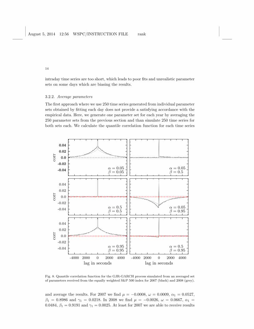
3.2.2. Average parameters

The first approach where we use 250 time series generated from individual parameter

sets obtained by fitting each day does not provide a satisfying accordance with the

empirical data. Here, we generate one parameter set for each year by averaging the

250 parameter sets from the previous section and than simulate 250 time series for

both sets each. We calculate the quantile correlation function for each time series

-0.04

-0.02

0.0

0.02

0.04

-0.04

-0.02

0.0

0.02

0.04

corr

-0.04

-0.02

0.0

0.02

0.04

corr

-0.04

-0.02

0.0

0.02

0.04

corr

-4000 2000 0 2000 4000

lag in seconds-4000 2000 0 2000 4000

lag in seconds

α = 0.05β = 0.05

α = 0.05β = 0.5

α = 0.5β = 0.5

α = 0.05β = 0.95

α = 0.95β = 0.95

α = 0.5β = 0.95

Fig. 8. Quantile correlation function for the GJR-GARCH process simulated from an averaged set

of parameters received from the equally weighted S&P 500 index for 2007 (black) and 2008 (grey).

and average the results. For 2007 we find µ = −0.0008, ω = 0.0009, α1 = 0.0527,

β1 = 0.8986 and γ1 = 0.0218. In 2008 we find µ = −0.0026, ω = 0.0667, α1 =

0.0484, β1 = 0.9191 and γ1 = 0.0025. At least for 2007 we are able to receive results


15

which on an absolute scale reproduce the empirical data rather well. However, we

still observe the qualitative discrepancies especially for the (0.05, 0.5) and (0.5, 0.95)

probabilities. The asymmetry is clearly visible and we find a normalized difference

between positive and negative lags of 4%. For 2008 we obtain a ten times smaller

asymmetry parameter γ1 in comparison to 2007. As the asymmetry parameter can

be negative or positive between the trading days they can compensate to nearly

zero. Thus, we observe no significant asymmetries for 2008.

Both approaches to fit the GJR-GARCH to the empirical intraday data fail to

deliver satisfying results.

4. Conclusion

The quantile correlation function gives a detailed picture of the temporal depen-

dencies in the underlying time series. It provides information which goes beyond

the autocorrelation of the absolute or squared returns and uncovers asymmetries in

the lagged correlations, which are connected to the leverage effect.

Beyond its usefulness for analyzing empirical time series it is a powerful tool to

find subtle differences in time series obtained from stochastic processes which are

designed to reproduce certain features. As an example we studied two stochastic

processes of the GARCH family with asymmetry parameters and found differences

compared to empirical data. It is beyond the scope of this paper to investigate every

stochastic process, see Bollerslev (2008) for an overview of GARCH type processes.

However, we advertize the reader to use the quantile correlation function to study

his favorite stochastic process and its temporal dependencies in more detail. In

general the quantile correlation function can serve as a sensitive tool to examine

the agreement between stochastic processes and empirical time series.

5. Acknowledgments

The work of H. Dette has been supported in part by the Collaborative Research

Center “Statistical modeling of nonlinear dynamic processes” (SFB 823, Teilprojekt

A1 and C1) of the German Research Foundation (DFG).


16

References

Yacine Aıt-Sahalia, Jianqing Fan, and Yingying Li. The leverage effect puzzle: Disentan-gling sources of bias at high frequency. Journal of Financial Economics, 109(1):224–249, 2013.

A. Cevdet Aydemir, Michael Gallmeyer, and Burton Hollifield. Financial leverage doesnot cause the leverage effect. AFA 2007 Chicago Meetings Paper, 2006.

Fischer Black. Studies of stock price volatility changes. In Proceedings of the 1976 Meetingsof the American Statistical Association, Business and Economics Statistics Section,pages 177–181, 1976.

Tim Bollerslev. Generalized Autoregressive Conditional Heteroskedasticity. Journal ofEconometrics, 31:307–327, 1986.

Tim Bollerslev. Glossary to ARCH (GARCH). CREATES Research Paper, 49, 2008.Pierre Cizeau, Yanhui Liu, Martin Meyer, C.-K. Peng, and H. Eugene Stanley. Volatility

distribution in the S&P500 stock index. Physica A, 245:441–445, 1997.Peter K. Clark. A Subordinated Stochastic Process Model with Finite Variance for Spec-

ulative Prices. The Econometric Society, 41(1):135–155, 1973.Holger Dette, Marc Hallin, Tobias Kley, and Stanislav Volgushev. Of Copulas, Quan-

tiles, Ranks and Spectra an L1-approach to spectral analysis. arXiv:1111.7205v1,to appear in: Bernoulli, 2011.

Zhuanxin Ding, Clive W.J. Granger, and Robert F. Engle. A long memory property ofstock market returns and a new model. Journal of Empirical Finance, 1(1):83–106,June 1993.

Robert F. Engle. Autoregressive Conditional Heteroscedasticity with Estimates of theVariance of United Kingdom Inflation. Econometrica, 50(4):987–1007, 1982.

Stephen Figlewski and Xiaozu Wang. Is the ”Leverage Effect” a Leverage Effect? FinanceWorking Papers, 2000. URL http://hdl.handle.net/2451/26702.

Alexios Ghalanos. rugarch: Univariate GARCH models., 2014. R package version 1.3-1.Lawrence R. Glosten, Ravi Jagannathan, and David E. Runkle. On the relation between

the expected value and the volatility of the nominal excess return on stocks. TheJournal of Finance, 48(5):1779–1801, 1993.

Andreas Hagemann. Robust Spectral Analysis. pages 1–50, 2013. URLhttp://arxiv.org/abs/1111.1965.

Benjamin Kedem. Binary Time Series. Lecture Notes in Pure and Applied Mathematics,52, 1980.

Roger Koenker. Quantile Regression. Econometric Society Monographs. Cambridge Uni-versity Press, 2005.

Ta-Hsin Li. Laplace Periodogram for Time Series Analysis. Journal of the AmericanStatistical Association, 103(482):757–768, June 2008.

Ta-Hsin Li. Quantile Periodograms. Journal of the American Statistical Association, 107(498):765–776, June 2012.

Oliver Linton and Yoon-Jae Whang. The quantilogram: With an application to evaluatingdirectional predictability. Journal of Econometrics, 141(1):250–282, 2007.

Yanhui Liu, Pierre Cizeau, Martin Meyer, C.-K. Peng, and H. Eugene Stanley. Correla-tions in economic time series. Physica A, 245:437–440, 1997.

Benoit Mandelbrot. The variation of certain speculative prices. The Journal of Business,36(4):394–419, 1963.

Frederick C. Mills. The Behavior of Prices. National Bureau of Economic Research, Inc.,New York, 1927.


17

Wesley C. Mitchell. The Making and Using of Index Numbers. Bulletin of the U.S. Bureauof Labor Statistics, 173, 1915.

Daniel B. Nelson. Conditional Heteroskedasticity in Asset Returns: A New Approach.Econometrica, 59(2):347–370, 1991.

Maurice Oliver. Les Nombres indices de la variation des prix. PhD thesis, Paris, 1926.Adrian Pagan. The econometrics of financial markets. Journal of Empirical Finance, 3

(1):15–102, 1996.Pierre-Alain Reigneron, Romain Allez, and J.P. Bouchaud. Principal regression analysis

and the index leverage effect. Physica A, 390(17):3026–3035, 2011.Minxian Yang. Normal Log-normal Mixture: Leptokurtosis, Skewness and Applications.

Econometric Society 2004 Australasian Meetings, 2004.

Documents

Thilo A. Schmitt, Rudi Schäfer, Holger Dette, Thomas … · SFB 823 Quantile correlations: Uncovering temporal dependencies in financial time series Discussion Paper Thilo A. Schmitt,