Embed Size (px)
Citation preview
arX
iv:1
102.
4885
v1 [
cs.D
M]
24 F
eb 2
011
The Tower of Hanoi problem on Pathh graphs
Daniel Berend
Departments of Mathematics and Computer Science, Ben-Gurion University, Beer-Sheva, Israel
Amir Sapir
Department of Software Systems, Sapir College, Western Negev, Israel 1 and
The Center for Advanced Studies in Mathematics at Ben-Gurion University, Beer-Sheva, Israel
Shay Solomon
Department of Computer Science, Ben-Gurion University, Beer-Sheva, Israel
Abstract
The generalized Tower of Hanoi problem with h ≥ 4 pegs is known to require a sub-exponentiallyfast growing number of moves in order to transfer a pile of n disks from one peg to another. In thispaper we study the Pathh variant, where the pegs are placed along a line, and disks can be movedfrom a peg to its nearest neighbor(s) only.
Whereas in the simple variant there are h(h−1)/2 possible bi-directional interconnections amongpegs, here there are only h − 1 of them. Despite the significant reduction in the number of inter-connections, the number of moves needed to transfer a pile of n disks between any two pegs alsogrows sub-exponentially as a function of n.
We study these graphs, identify sets of mutually recursive tasks, and obtain a relatively tightupper bound for the number of moves, depending on h, n and the source and destination pegs.
Keywords: Tower of Hanoi, path graphs, analysis of algorithms
1 Introduction
In the well-known Tower of Hanoi problem, proposed over a hundred years ago by
Lucas [20], a player is given 3 pegs and a certain number n of disks of distinct sizes,
and is required to transfer them from one peg to another. Initially all disks are stacked
(composing a tower) on the first peg (the source) ordered monotonically by size, with the
smallest at the top and the largest at the bottom. The goal is to transfer them to the
third peg (the destination), moving only topmost disks, and never placing a disk on top
of a smaller one. The well-known recursive algorithm that accomplishes this task requires
2n − 1 steps, and is the unique optimal algorithm for the problem. The educational
aspects of the Tower of Hanoi puzzle have been reinforced recently, by a series of papers
1 Research supported in part by the Sapir Academic College, Israel.
1
by Minsker ([23, 24, 25]), composing variants for the sake of studying their combinatorial
as well as algorithmic aspects.
Work on this problem still goes on, studying properties of solution instances, as well
as variants of the original problem. Connections between Pascal’s triangle, the Sierpinski
gasket and the Tower of Hanoi are established in [16], and to some classical numbers
in [18]. In [1] it is shown that, with a certain way of coding the moves, a string which
represents an optimal solution is square-free. This line is extended in [2]. Another
direction was concerned with various generalizations, such as having any initial and final
configurations [14], assigning colors to disks (cf. [21] and [22] for recent papers on the
subject), and relaxing the placement rule of disks by allowing a disk to be placed on top
of a smaller one under prescribed conditions [9, 10, 11].
A natural extension of the original problem is obtained by adding pegs. One of the
earliest versions is “The Reve’s Puzzle” [12, pp. 1-2]. There it was presented in a
limited form: 4 pegs and specified numbers of disks. The general setup of the problem,
with any number h > 3 of pegs and any number of disks, was suggested in [28], with
solutions in [29] and [15], shown recently to be identical [17]. An analysis of the algorithm
reveals, somewhat surprisingly, that the solution grows sub-exponentially, at the rate of
Θ(√n2
√2n) for h = 4 (cf. [30]). The lower bound issue was considered in [32] and [8],
where it has been shown that the minimal number of moves grows roughly at the same
rate.
An imposition of movement restrictions among pegs generates many variants, and
calls for representing variants by digraphs, where a vertex designates a peg, and an
arc represents the permission to move a disk in the appropriate direction. In [3, 13],
the uni-directional cyclic 3-peg variant (Cyclic3) has been studied, and the average
distance between the nodes – in [31]. In [27], the “three-in-a-row” arrangement (Path3) is
discussed. A unified treatment of all 3-peg variants is given in [26]. The (uni-directional)
Cyclic4 is discussed for the first time in [27], and [30] studies other 4-peg variants:
Star4 and Path4, presenting a sub-exponential algorithm for Star4. The Cyclich for
any number of pegs h ≥ 4 has been studied in [6] and proved to be exponential for any
specified h. Identification of the longest task, for certain variants, has been resolved in
[7].
The only requirement for the problem to be solved for any number of disks is that
the variant is represented by a strongly-connected directed graph. An interesting line of
2
research has been taken in [19], [4], and [5], where non-strongly-connected graphs are
being studied.
In this paper we study the Pathh variant, with a fixed number h ≥ 4 of pegs, whose
complexity issue has been left open. We devise an efficient algorithm which moves a
column of n disks between any pair of pegs, and supply an explicit subexponential upper
bound on the number of moves, for each h.
Notations and definitions are given in Section 2, the main results in Section 3, the
proof of the 4-peg case in Section 4 and that of the general case in Section 5.
2 Preliminaries
We study the Pathh (a.k.a. h-in-a-row) variant, with a fixed number h ≥ 4 of pegs.
We denote the pegs of Pathh, from left to right, by 1, . . . , h. Let the sizes of the disks
be 1, 2, . . . , n. For convenience, we identify the name of a disk with its size.
For the statements and algorithms of the paper, it is required to introduce the notion of
a block — a set of disks of consecutive sizes. The minimum (respectively, maximum) size
of a disk in a block B is denoted by Bmin (resp., Bmax), and the number Bmax−Bmin+1
of disks in B — by |B|. A block B is lighter than another block B′ if Bmax < B′min.
A configuration is a legal distribution of the n disks among the h pegs. A perfect
configuration is one in which all the disks reside on the same peg. Such a configuration
is denoted by Rh,i,n, where h is the number of pegs, i the peg holding the disks, and n
the number of disks.
For a sequence of movesM , henceforth move-sequence, we denote by M−1 the reverse
move-sequence, comprising the moves that cause the reverse effect. That is, the order
of the moves is reversed and each move of the original sequence is reversed. Clearly, if
applying M to configuration C1 results in reaching configuration C2, then applying M−1
to C2 results in configuration C1. (Note that this is true if and only if the peg structure
is a graph; for digraphs in general this is not true.)
A problem instance, henceforth a task, is given by a pair of configurations, an initial
configuration C1 and a final configuration C2, where we are required to move from C1
to C2 in a minimal number of moves. The task, as well as a minimal-length solution of
it, is denoted by C1 → C2, and the minimum number of moves needed to get from C1
to C2 is denoted by |C1 → C2|.
3
In this paper we focus on perfect tasks — problem instances whose initial and final
configurations are both perfect. The peg associated with the initial (respectively, final)
configuration of a perfect task is naturally referred to as the source (resp., destination).
Clearly, for any positive integers h, n and 1 ≤ i < j ≤ h, we have |Rh,i,n → Rh,j,n| =|Rh,j,n → Rh,i,n|. We shall henceforth restrict our attention in the sequel to tasks in
which the source peg is to the left (i.e. has a lower peg index) of the destination peg.
For n ≥ 1, denote by Path(h, n) the minimal number of moves which suffices for
transferring a block of size n between all pairs of perfect configurations in Pathh, namely,
Path(h, n) = max1≤i<j≤h
|Rh,i,n → Rh,j,n| .
For a real number x, let round(x) be the integer closest to x (where round(x) = ⌈x⌉for x = n + 0.5). For a pair of positive integers p and q, with p < q, we denote the set
{p, . . . , q} by [p, q], and [1, . . . , q] by [q]. In what follows, we do not distinguish between a
move-sequence and an algorithm generating it, if this does not lead to a misunderstanding.
3 Main results
The main question the paper addresses is: what is the complexity of Path(h, n)?
An upper bound is provided by
Theorem 3.1 Path(h, n) ≤ Chnαh · 3θh·n
1h−2
, for all h ≥ 3 and n, where:
θh = ((h− 2)!)1
h−2 ,
αh = h−3h−2
,
Ch = (h−2)·δh−3
θh,
(δ = 11
32−(1/30)1/3
).
In particular, Path(h, n) grows subexponentially as a function of n for h ≥ 4.
Of course, as a lower bound for Path(h, n) one may use any lower bound for the
number of moves required to move a tower of size n from one peg to another over the
complete graph on h vertices. By [8], such a lower bound is given by 2(1+o(1))(n(h−2)!)1
h−2,
which is “not very far” from our upper bound for Path(h, n).
The following theorem identifies the hardest perfect task for the particular case h = 4.
It also provides a tighter upper bound for Path4 than the one given in Theorem 3.1.
Theorem 3.2 For every n ≥ 1:
4
(a) |R4,i,n → R4,j,n| < |R4,1,n → R4,4,n| for 1 ≤ i < j ≤ 4, (i, j) 6= (1, 4). In
particular, Path(4, n) = |R4,1,n → R4,4,n|.
(b) Path(4, n) < 1.6√n3
√2n.
4 Proof of Theorem 3.2
4.1 On the relation between various tasks in Path4
We start with a result of some independent interest, which holds for general h.
Lemma 4.1 Let C be a configuration with n ≥ 1 disks, arranged arbitrarily on pegs
1, . . . , h− 2, with pegs h− 1 and h empty. Then:
|C → Rh,h−2,n| < |C → Rh,h,n|, |C → Rh,h−1,n| < |C → Rh,h,n| .
Proof: We detail the proof for |C → Rh,h−2,n| < |C → Rh,h,n|. The proof for the
second inequality is similar.
The proof is by induction on n. The basis n = 1 is trivial. Let n ≥ 2, assume that the
statement holds for up to n− 1 disks, and let C be a configuration as in the statement
of the lemma and M a move-sequence transferring from C to Rh,h,n. Before the last
move of disk n (to peg h), a configuration C ′, in which all n − 1 disks 1, 2, . . . , n − 1
are distributed among pegs 1, . . . , h − 2, is reached. Let M ′ (respectively, M ′′) be the
subsequence of M , consisting of all moves that come before (resp., after) the last move of
disk n. Notice that M ′′ transfers from C ′ (considered as a configuration of n−1 disks) to
Rh,h,n−1. By the induction hypothesis, there exists a move-sequence M ′′h−2 that transfers
from C ′ to Rh,h−2,n−1, which is strictly shorter than M ′′. Let M ′h−2 be the move-sequence
obtained from M ′ by omitting all moves disk n makes after reaching peg h − 2 for the
first time. Concatenating M ′h−2 with M ′′
h−2, we obtain a legal move-sequence, strictly
shorter than M , transferring from C to Rh,h−2,n. The required result follows.
Due to symmetries, there are actually only four essentially distinct perfect tasks in
Path4: R4,1,n → R4,2,n, R4,1,n → R4,3,n, R4,1,n → R4,4,n, and R4,2,n → R4,3,n. By
Lemma 4.1, taking h = 4 and C to be various perfect configurations, we obtain for any
n ≥ 1
• |R4,1,n → R4,2,n| < |R4,1,n → R4,4,n|.
• |R4,2,n → R4,3,n| < |R4,2,n → R4,4,n| = |R4,1,n → R4,3,n| < |R4,1,n → R4,4,n|.
5
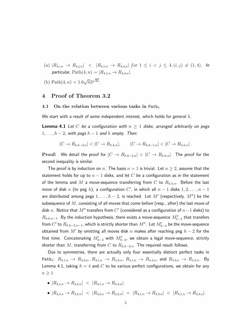
These inequalities establish part (a) of Theorem 3.2.
In Table 1 we present the (distinct) numbers |R4,i,n → R4,j,n| for 1 ≤ n ≤ 11. The
entries have been calculated by finding the distance between the vertices R4,i,n and R4,j,n
in the graph of all configurations of n disks on Path4 using breadth-first search.
tasks
disks 2→ 3 1→ 2 1→ 3 1→ 4 1→4√n3
√
2n
1 1 1 2 3 0.6342 4 4 6 10 0.7863 7 9 12 19 0.7444 14 18 22 34 0.7605 23 29 36 57 0.7906 34 44 54 88 0.7997 53 69 78 123 0.7628 78 96 112 176 0.7689 105 133 158 253 0.798
10 138 182 212 342 0.79511 187 241 272 449 0.783
Table 1: The minimal numbers of moves for the 4 different perfect tasks in Path4
The table prompts
Question 1 Is it the case that |R4,1,n → R4,2,n| < |R4,1,n → R4,3,n| and |R4,2,n →R4,3,n| < |R4,1,n → R4,2,n| for all n ≥ 3?
Both of these inequalities seem intuitively quite plausible.
4.2 Upper bound for Path(4, n)
In this subsection we present the algorithm FourMove for moving a block B of size n from
peg 1 to peg 4 in Path4, requiring no more than 1.6√n3
√2n moves. By Theorem 3.2(a),
this will imply Theorem 3.2(b). The description of FourMove is given in Algorithm 1.
Prior to its main stages, FourMove partitions B into three: a block containing the
smallest disks, a block containing the larger ones, and a block containing a single disk
– the largest one. These blocks are denoted Bs, Bl, {Bmax} respectively, with m =
|Bl
⋃{Bmax}|. Thus Bs = [Bmin, Bmax−m] and Bl = [Bmax−m+1, Bmax− 1]. In the
three principal stages that follow: Spread, Circular shift and Accumulate, the moves are
done based on these blocks. In Spread, Bs is transferred to the farthest peg – number 4,
6
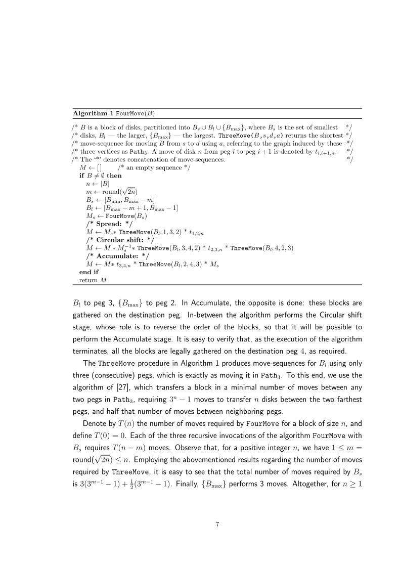
Algorithm 1 FourMove(B)
/* B is a block of disks, partitioned into Bs ∪Bl ∪ {Bmax}, where Bs is the set of smallest *//* disks, Bl — the larger, {Bmax} — the largest. ThreeMove(B,s,d,a) returns the shortest *//* move-sequence for moving B from s to d using a, referring to the graph induced by these *//* three vertices as Path3. A move of disk n from peg i to peg i+ 1 is denoted by ti,i+1,n. *//* The ‘*’ denotes concatenation of move-sequences. */
M ← [ ] /* an empty sequence */if B 6= ∅ thenn← |B|m← round(
√2n)
Bs ← [Bmin, Bmax −m]Bl ← [Bmax −m+ 1, Bmax − 1]Ms ← FourMove(Bs)/* Spread: */M ←Ms∗ ThreeMove(Bl, 1, 3, 2) * t1,2,n/* Circular shift: */M ←M ∗M−1
s ∗ ThreeMove(Bl, 3, 4, 2) * t2,3,n * ThreeMove(Bl, 4, 2, 3)/* Accumulate: */M ←M∗ t3,4,n * ThreeMove(Bl, 2, 4, 3) * Ms
end ifreturn M
Bl to peg 3, {Bmax} to peg 2. In Accumulate, the opposite is done: these blocks are
gathered on the destination peg. In-between the algorithm performs the Circular shift
stage, whose role is to reverse the order of the blocks, so that it will be possible to
perform the Accumulate stage. It is easy to verify that, as the execution of the algorithm
terminates, all the blocks are legally gathered on the destination peg 4, as required.
The ThreeMove procedure in Algorithm 1 produces move-sequences for Bl using only
three (consecutive) pegs, which is exactly as moving it in Path3. To this end, we use the
algorithm of [27], which transfers a block in a minimal number of moves between any
two pegs in Path3, requiring 3n − 1 moves to transfer n disks between the two farthest
pegs, and half that number of moves between neighboring pegs.
Denote by T (n) the number of moves required by FourMove for a block of size n, and
define T (0) = 0. Each of the three recursive invocations of the algorithm FourMove with
Bs requires T (n−m) moves. Observe that, for a positive integer n, we have 1 ≤ m =
round(√2n) ≤ n. Employing the abovementioned results regarding the number of moves
required by ThreeMove, it is easy to see that the total number of moves required by Bs
is 3(3m−1 − 1) + 12(3m−1 − 1). Finally, {Bmax} performs 3 moves. Altogether, for n ≥ 1
7
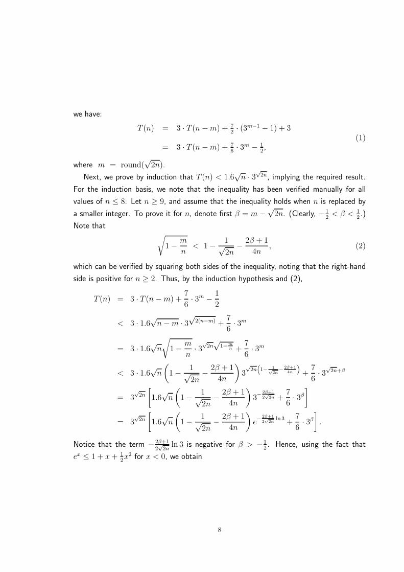
we have:
T (n) = 3 · T (n−m) + 72· (3m−1 − 1) + 3
= 3 · T (n−m) + 76· 3m − 1
2,
(1)
where m = round(√2n).
Next, we prove by induction that T (n) < 1.6√n · 3
√2n, implying the required result.
For the induction basis, we note that the inequality has been verified manually for all
values of n ≤ 8. Let n ≥ 9, and assume that the inequality holds when n is replaced by
a smaller integer. To prove it for n, denote first β = m−√2n. (Clearly, −1
2< β < 1
2.)
Note that√
1− m
n< 1− 1√
2n− 2β + 1
4n, (2)
which can be verified by squaring both sides of the inequality, noting that the right-hand
side is positive for n ≥ 2. Thus, by the induction hypothesis and (2),
T (n) = 3 · T (n−m) +7
6· 3m − 1
2
< 3 · 1.6√n−m · 3
√2(n−m) +
7
6· 3m
= 3 · 1.6√n√
1− m
n· 3
√2n√
1−mn +
7
6· 3m
< 3 · 1.6√n(1− 1√
2n− 2β + 1
4n
)3√2n
(
1− 1√2n
− 2β+14n
)
+7
6· 3
√2n+β
= 3√2n
[1.6√n
(1− 1√
2n− 2β + 1
4n
)3− 2β+1
2√
2n +7
6· 3β]
= 3√2n
[1.6√n
(1− 1√
2n− 2β + 1
4n
)e− 2β+1
2√
2nln 3
+7
6· 3β].
Notice that the term − 2β+1
2√2n
ln 3 is negative for β > −12. Hence, using the fact that
ex ≤ 1 + x+ 12x2 for x < 0, we obtain
8
T (n)
1.6·3√
2n<
√n(1− 1√
2n− 2β+1
4n
)(1− 2β+1
2√2n
ln 3 + (2β+1)2 ln2 316n
)+ 35
48· 3β
=(√
n− 1√2− (2β+1) ln 3
2√2
)
+(−2β+1
4√n+ (2β+1) ln 3
4√n
+ (2β+1)2 ln2 316
√n
)
+(
(2β+1)2 ln 3
8√2·n − (2β+1)2 ln2 3
16√2·n − (2β+1)3 ln2 3
64n√n
)+ 35
48· 3β
=(√
n− 1√2− (2β+1) ln 3
2√2
)
+(−2β+1
4√n+ (2β+1) ln 3
4√n
+ (2β+1)2 ln2 316
√n
+ (2β+1)2 ln2 3
16√2·n
)
+(
(2β+1)2 ln 3
8√2·n − (2β+1)2 ln2 3
8√2·n − (2β+1)3 ln2 3
64n√n
)+ 35
48· 3β.
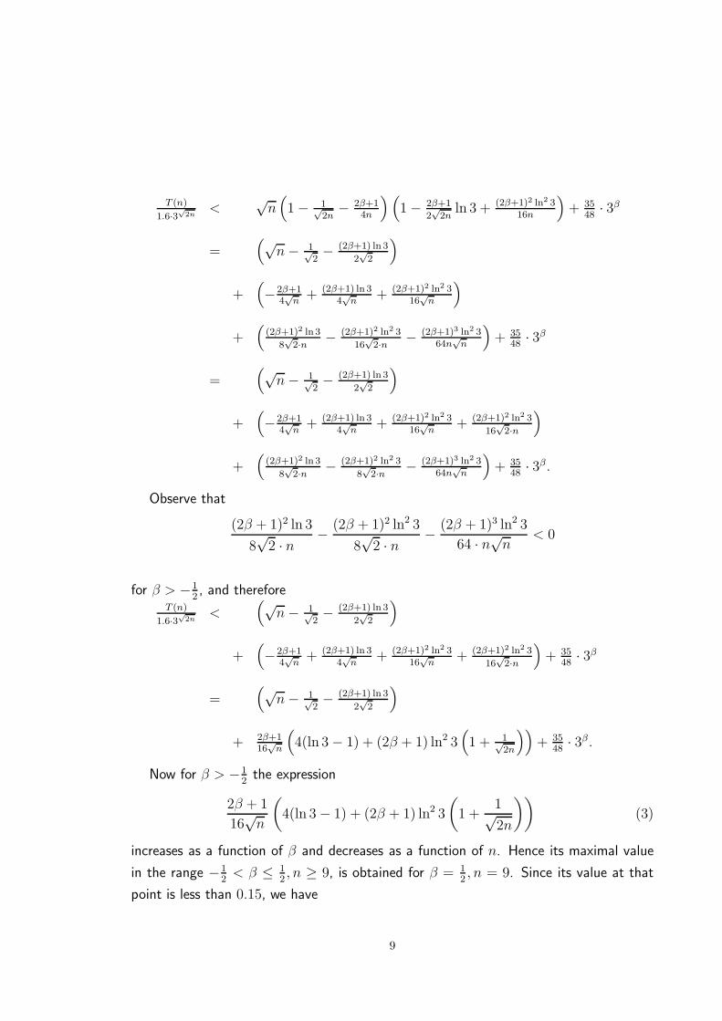
Observe that
(2β + 1)2 ln 3
8√2 · n
− (2β + 1)2 ln2 3
8√2 · n
− (2β + 1)3 ln2 3
64 · n√n < 0
for β > −12, and therefore
T (n)
1.6·3√
2n<
(√n− 1√
2− (2β+1) ln 3
2√2
)
+(−2β+1
4√n+ (2β+1) ln 3
4√n
+ (2β+1)2 ln2 316
√n
+ (2β+1)2 ln2 3
16√2·n
)+ 35
48· 3β
=(√
n− 1√2− (2β+1) ln 3
2√2
)
+ 2β+116
√n
(4(ln 3− 1) + (2β + 1) ln2 3
(1 + 1√
2n
))+ 35
48· 3β.
Now for β > −12the expression
2β + 1
16√n
(4(ln 3− 1) + (2β + 1) ln2 3
(1 +
1√2n
))(3)
increases as a function of β and decreases as a function of n. Hence its maximal value
in the range −12< β ≤ 1
2, n ≥ 9, is obtained for β = 1
2, n = 9. Since its value at that
point is less than 0.15, we have
9
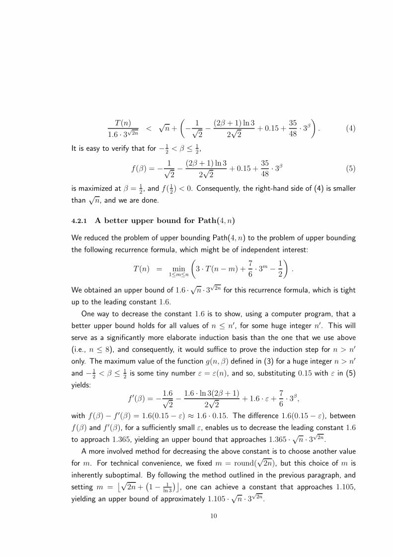
T (n)
1.6 · 3√2n
<√n+
(− 1√
2− (2β + 1) ln 3
2√2
+ 0.15 +35
48· 3β). (4)
It is easy to verify that for −12< β ≤ 1
2,
f(β) = − 1√2− (2β + 1) ln 3
2√2
+ 0.15 +35
48· 3β (5)
is maximized at β = 12, and f(1
2) < 0. Consequently, the right-hand side of (4) is smaller
than√n, and we are done.
4.2.1 A better upper bound for Path(4, n)
We reduced the problem of upper bounding Path(4, n) to the problem of upper bounding
the following recurrence formula, which might be of independent interest:
T (n) = min1≤m≤n
(3 · T (n−m) +
7
6· 3m − 1
2
).
We obtained an upper bound of 1.6 ·√n · 3√2n for this recurrence formula, which is tight
up to the leading constant 1.6.
One way to decrease the constant 1.6 is to show, using a computer program, that a
better upper bound holds for all values of n ≤ n′, for some huge integer n′. This will
serve as a significantly more elaborate induction basis than the one that we use above
(i.e., n ≤ 8), and consequently, it would suffice to prove the induction step for n > n′
only. The maximum value of the function g(n, β) defined in (3) for a huge integer n > n′
and −12< β ≤ 1
2is some tiny number ε = ε(n), and so, substituting 0.15 with ε in (5)
yields:
f ′(β) = −1.6√2− 1.6 · ln 3(2β + 1)
2√2
+ 1.6 · ε+ 7
6· 3β,
with f(β)− f ′(β) = 1.6(0.15 − ε) ≈ 1.6 · 0.15. The difference 1.6(0.15 − ε), between
f(β) and f ′(β), for a sufficiently small ε, enables us to decrease the leading constant 1.6
to approach 1.365, yielding an upper bound that approaches 1.365 · √n · 3√2n.
A more involved method for decreasing the above constant is to choose another value
for m. For technical convenience, we fixed m = round(√2n), but this choice of m is
inherently suboptimal. By following the method outlined in the previous paragraph, and
setting m =⌊√
2n+(1− 1
ln 3
)⌋, one can achieve a constant that approaches 1.105,
yielding an upper bound of approximately 1.105 · √n · 3√2n.
10
5 Proof of Theorem 3.1
The proof of Theorem 3.1 is organized as follows. Generally, we would like to show how
one can move a column of n disks from any source peg s to any destination peg d such
that the number of moves is bounded above as the theorem states. For simplicity, we
start by presenting an algorithm for the case where s = 1, d = h. This will be done in
Section 5.1. Then we present an algorithm for the general case (Section 5.2). We note
that, in fact, the first algorithm does employ the second. An important point in both
cases is a partitioning of the set of disks to blocks, which will be discussed in Section 5.3.
Time analysis of the two algorithms will be provided in Section 5.4.
5.1 Moving disks between the farthermost pegs
Here we present FarthestMove (Algorithm 2), designed to move a block B of n disks
between the two farthest pegs in Pathh, where h ≥ 3.
We partition B in some way to blocks B1(h,B), B2(h,B), . . . , Bh−1(h,B) of disks.
Whenever h and B are implied by the context, we write Bi instead of Bi(h,B). The
block B1 consists of the smallest n1 disks 1, 2, . . . , n1, the block B2 — of the n2 next
smallest disks n1 + 1, n1 + 2, . . . , n1 + n2, and so forth. Similarly to the shorthand used
when denoting blocks, we may write ni (with a possible superscript) instead of ni(h, n).
For any i ∈ [h− 1], let B(i) =⋃h−1
j=i Bj and n(i) = |B(i)| = Σh−1j=i nj , where nj = |Bj |.
(Note that B(1) = B and n(1) = n.)
The determination of the sizes ni is crucial for the number of moves the algorithm
makes, and will be explained later. However, for the algorithm to work correctly, it is
only required for Bh−1 to consist of the single disk Bmax — the largest. The algorithm
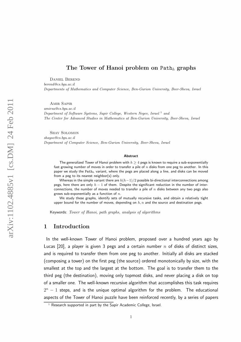
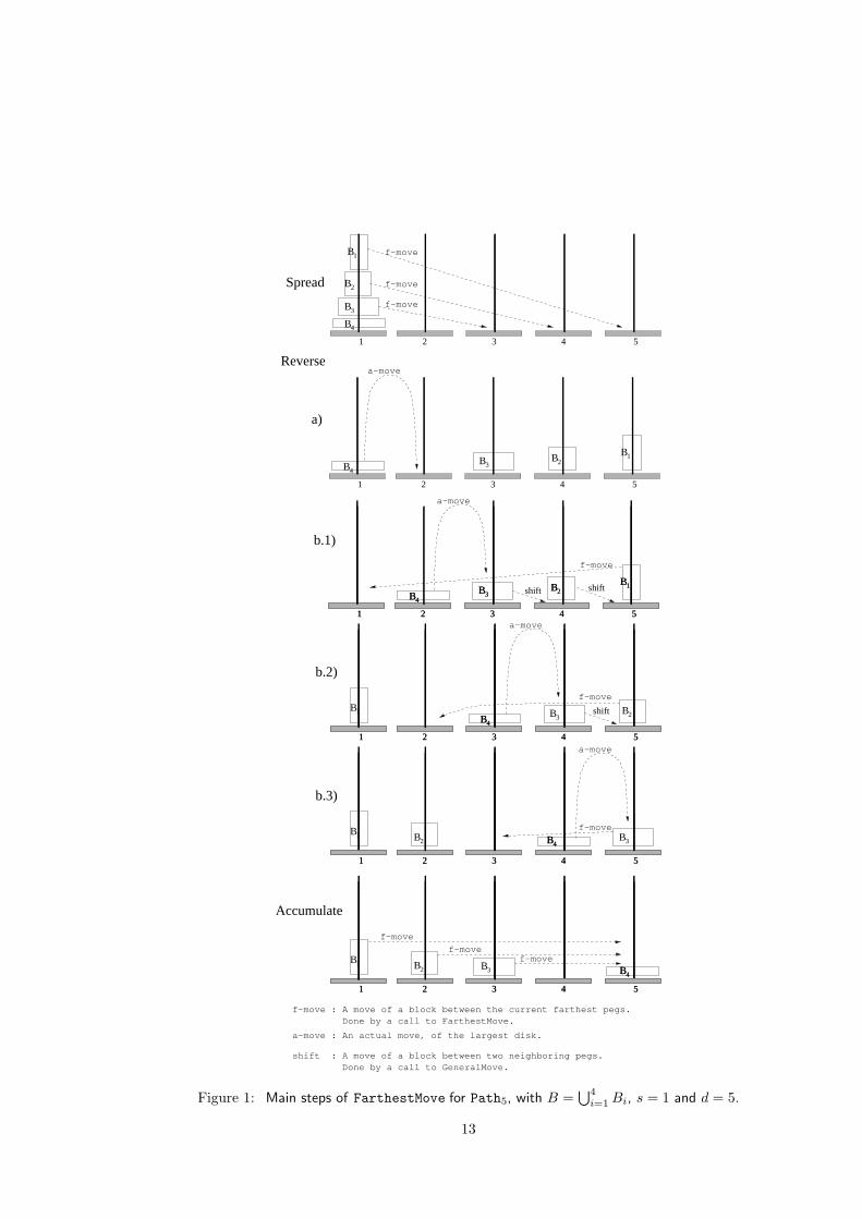
consists of three phases (see Figure 1 for an illustration):
• Spread: Move the h− 2 (= d− s− 1) first blocks B1, . . . , Bh−2 from the source
peg s to pegs d, . . . , d− h + 3, respectively. It consists of h− 2 iterations. At the
j-th iteration, j ∈ [h−2], block Bj is (recursively) moved from s to d− j+1, using
the set [1, d − j + 1] of available pegs. (Note that the 1-disk block Bh−1 has not
been moved from s to s+ 1. It is more convenient for us to view this move as the
first move of the next stage.)
• Reverse: The role of this phase is to reverse the positions of the h− 1 blocks on
the h pegs, i.e., a block residing, at the beginning of this phase, on peg s + i − 1
11
reaches, at the end of the phase, its reflected position — peg d− i+ 1. The phase
starts by moving the last block Bh−1 from s to s + 1. Then, h − 2 rounds are
carried out, each of which brings the next larger block to its reflected position. The
following highlights the way each round j achieves its goal:
– Before this round, blocks B1, . . . , Bj−1 are on pegs s, . . . , s+j−2, respectively;peg s+j−1 is vacant; blocks Bj , . . . , Bh−1 are on pegs d, . . . , s+j, respectively.
– Block Bj is moved from d to s+ j − 1.
– Blocks Bj+1, . . . , Bh−1 are each shifted one peg to the right.
– At the end of the round, blocks B1, . . . , Bj are on pegs s, . . . , s+ j−1, respec-
tively; peg s+ j is vacant; blocks Bj+1, . . . , Bh−1 are on pegs d, . . . , s+ j + 1,
respectively.
Thus, as a result of this phase, block Bh−1 is moved from s to d and, for each
j ∈ [h− 2], block Bj is moved from peg d− j+1 to the reflected position, namely,
peg s+ j − 1.
• Accumulate: The role of this phase is symmetrical to that of Spread, i.e., to
move the h− 2 first blocks Bh−2, . . . , B1 from pegs d− 2, . . . , s, respectively, to d.
Similarly, it consists of h− 2 iterations, where at the j-th iteration block Bh−1−j is
moved from s+ h− 2− j to d using the set [s+ h− 2− j, d] of available pegs.
It is easy to verify that, as the execution of the algorithm terminates, all the blocks are
legally gathered on d, as required. The formal description of the algorithm FarthestMove
is given in Algorithm 2.
5.2 Moving disks between any pegs
The general algorithm for moving a block of disks, between any two pegs s and d, in
Pathh, is presented here. For convenience we assume that s < d. This does not effect
the generality of the algorithm since, as was mentioned in Section 2, if M is a solution
of Rh,s,n → Rh,d,n, then M−1 is a solution of Rh,d,n → Rh,s,n.
The issue of partitioning the disk set is handled exactly as it was done in FarthestMove.
Algorithm GeneralMove consists of five phases: two spread phases, a phase in which the
remainder disks are moved, and two accumulate phases. The set of available pegs is
denoted by A, and its smallest and largest pegs by Amin and Amax, respectively.
12
2 31 4 52 31
4 52 31 4 52 31
52 31 4 52 31
52 31 4 52 31
2 31
52 31 4
54
5
4
4
4
B B142 4B 3B
4
B1
B
B
B3
4
2Spread
Reverse
B
4
B
B
4
B4
a)
B3B2B1B
4B
shift shift
b.1)
3B 2B1B
4B4
shift
b.2)
Accumulate
B 3B 2B 1B3B 2B 1B
3B 2B 1B
b.3)
f-move
f-move
f-move
a-move
f-move
f-move
f-movef-move
a-move
a-move
f-move
f-move
a-move
Done by a call to FarthestMove.f-move : A move of a block between the current farthest pegs.
a-move : An actual move, of the largest disk.
shift : A move of a block between two neighboring pegs. Done by a call to GeneralMove.
Figure 1: Main steps of FarthestMove for Path5, with B =⋃4
i=1 Bi, s = 1 and d = 5.
13
Algorithm 2 FarthestMove(B, s, d)
/* The procedure moves a block B from the leftmost peg s to the rightmost peg d. Prior *//* to its main stages, the block is partitioned into h− 1 blocks which are treated as ‘atomic *//* units’. At the first of the main stages, these blocks are spread along the pegs; at the *//* second – their order is reversed; at the third stage they are accumulated on the destination *//* peg. The procedure requires that s < d. If d− s = 1, then |B| ≤ 1. The ‘*’ denotes *//* concatenation of move-sequences. */
T ← [ ] /* initializing the result sequence */if B 6= ∅ thenh← d− s+ 1(B1, . . . , Bh−1) = Partition(h,B) /* Algorithm 5 below */
/* Spread: */for j ← 1 to h− 2 do/* At each step, the next block moves to the farthest available peg. */T ← T ∗ FarthestMove(Bj , s, d− j + 1)
end for
/* Reverse: */T ← T ∗ tBmax,s,s+1 /* Moving the largest disk once a peg to the right. */M ← [ ] /* Initializing the temporary move-sequence. */for j ← 1 to h− 2 do/* Block Bj moves to the peg on which it will stay for the rest of this phase. */Mf ← FarthestMove(Bj , s+ j − 1, d)M ←M ∗M−1
f
for i← j + 1 to h− 2 do/* Each block whose index is higher than j is shifted one peg to the right. */M ←M ∗ GeneralMove(Bi, d+ j − i, d+ j + 1− i, [s+ j, d+ j + 1− i])
end forT ← T ∗M ∗ tBmax,j+1,j+2 /* Moving the largest disk a peg to the right. */
end for
/* Accumulate: */for j ← 1 to h− 2 do/* At each step, the next block is gathered on the destination peg. */T ← T ∗ FarthestMove(Bh−1−j , s+ h− 2− j, d)
end forend ifreturn T
14
• LeftSpread: In this phase the s−Amin first blocks B1, . . . , Bs−Aminare taken from
peg s to pegs Amin, . . . , s − 1, respectively. It consists of s − Amin iterations. At
the j-th iteration, 1 ≤ j ≤ s − Amin, block Bj is (recursively) moved from s to
Amin + j − 1 using the set [Amin + j − 1, Amax] of available pegs.
• RightSpread: Here, the Amax − d next blocks are taken, from peg s to pegs
Amax, . . . , d + 1, respectively. At each iteration j, where 1 ≤ j ≤ Amax − d, block
Bs−Amin+j is moved from s to Amax − j + 1, using [s, Amax − j + 1]. Since at
each iteration the source and destination are at the opposite ends of the currently
available set of free pegs, the move is done using algorithm FarthestMove.
• MoveRemainder: In this phase, the remaining B(d− s) blocks are moved from
s to d. Since, as before, the source and destination are at the opposite sides of the
set [s, d] of available pegs, this is done by algorithm FarthestMove.
• LeftAccumulate: The role of this phase is symmetrical to that of RightSpread,
that is, move Bs−Amin+1, . . . , Bs+|A|−1−d from Amax, . . . , d+ 1 to d, respectively. It
consists of Amax−d iterations, where at iteration j, block Bs+|A|−d−j is moved from
d+ j to d using [s, d+ j]. Unlike RightSpread, the moves made in this phase are
not between the two farthest available pegs.
• RightAccumulate: This phase is symmetrical to LeftSpread, consisting of s−Amin iterations where, at the j-th iteration, Bs−j is moved from peg s − j to peg
d, using [s− j, Amax].
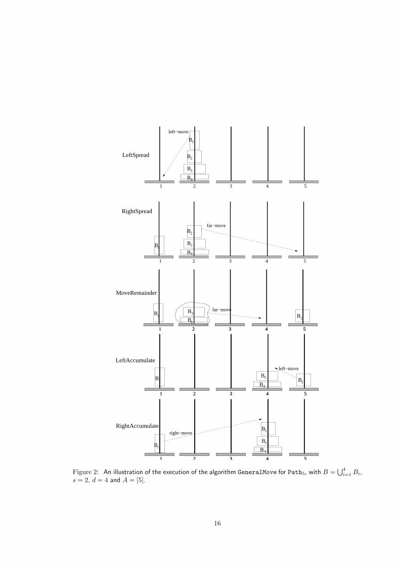
It is easy to verify that, as the algorithm terminates, all the blocks are legally gathered on
the destination peg d, as required (see Figure 2 for an illustration). The correctness proof
is omitted. The formal description of GeneralMove is given in Algorithm 3. Note that, if
the source and destination pegs are at the opposite sides of A, then GeneralMove does
the same as FarthestMove.
5.3 Partitioning the disks into blocks
In this section we discuss how to set the sizes of the blocks such that the number of
moves will be relatively low. The general idea is to view the h−1 blocks as ‘atomic’ units,
each occupying a single peg (except for when it is moved). During the process of moving a
block Bi from one peg s to another peg d, the other blocks stay intact. Furthermore, the
15
2
1 32 54
1 32 54
1 32 541 32 54
1 32 541 3 54
1 32 541 32 54
B2
B3
B
B3
B
B2
B1
1
B
B3
2
4B
LeftAccumulate
MoveRemainder
4
left−move
B
RightAccumulate
4
LeftSpread
RightSpread
B
B
B3
2
B1
left−move
far−move
B1 B2
B3
B
4
4
far−move
right−move
B
1
Figure 2: An illustration of the execution of the algorithm GeneralMove for Path5, with B =⋃4
i=1 Bi,
s = 2, d = 4 and A = [5].
16
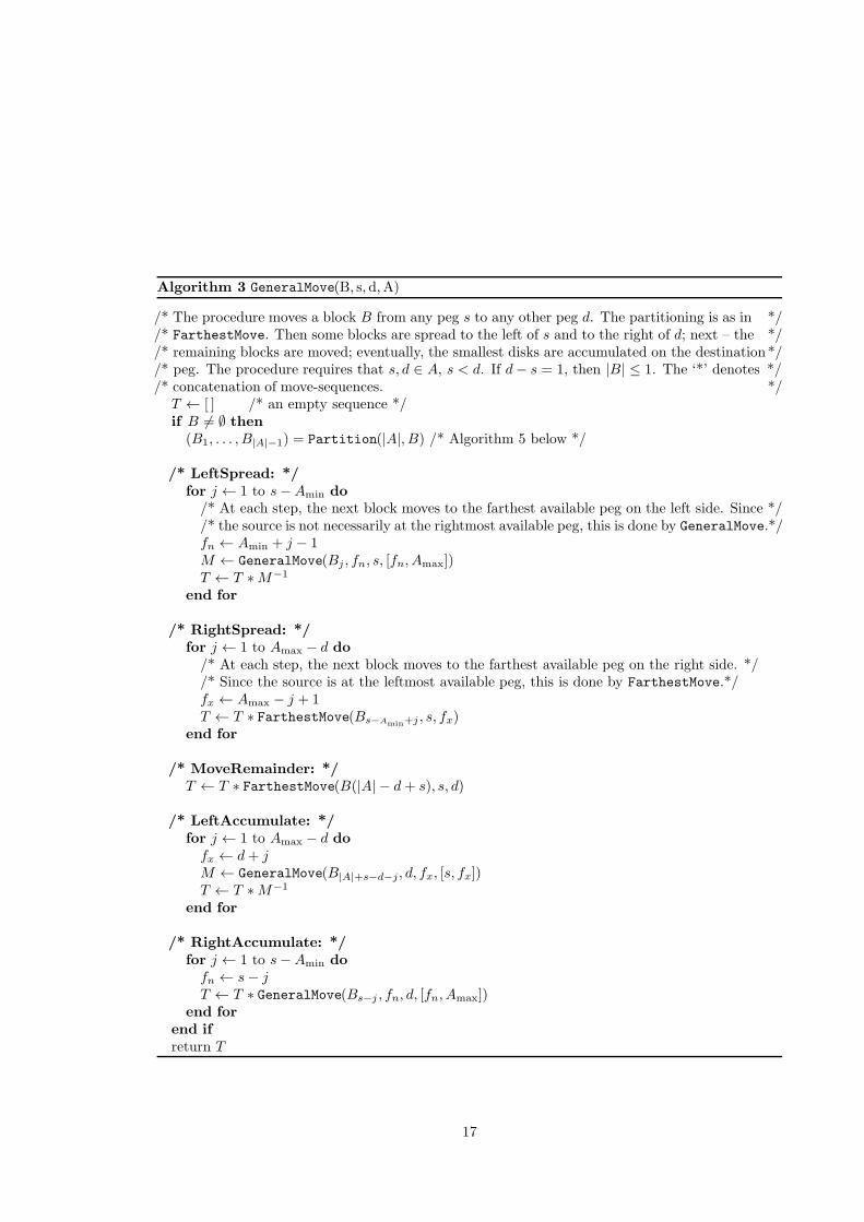
Algorithm 3 GeneralMove(B, s, d,A)
/* The procedure moves a block B from any peg s to any other peg d. The partitioning is as in *//* FarthestMove. Then some blocks are spread to the left of s and to the right of d; next – the *//* remaining blocks are moved; eventually, the smallest disks are accumulated on the destination*//* peg. The procedure requires that s, d ∈ A, s < d. If d− s = 1, then |B| ≤ 1. The ‘*’ denotes *//* concatenation of move-sequences. */
T ← [ ] /* an empty sequence */if B 6= ∅ then(B1, . . . , B|A|−1) = Partition(|A|, B) /* Algorithm 5 below */
/* LeftSpread: */for j ← 1 to s−Amin do/* At each step, the next block moves to the farthest available peg on the left side. Since *//* the source is not necessarily at the rightmost available peg, this is done by GeneralMove.*/fn ← Amin + j − 1M ← GeneralMove(Bj , fn, s, [fn, Amax])T ← T ∗M−1
end for
/* RightSpread: */for j ← 1 to Amax − d do/* At each step, the next block moves to the farthest available peg on the right side. *//* Since the source is at the leftmost available peg, this is done by FarthestMove.*/fx ← Amax − j + 1T ← T ∗ FarthestMove(Bs−Amin+j , s, fx)
end for
/* MoveRemainder: */T ← T ∗ FarthestMove(B(|A| − d+ s), s, d)
/* LeftAccumulate: */for j ← 1 to Amax − d dofx ← d+ j
M ← GeneralMove(B|A|+s−d−j, d, fx, [s, fx])T ← T ∗M−1
end for
/* RightAccumulate: */for j ← 1 to s−Amin dofn ← s− j
T ← T ∗ GeneralMove(Bs−j , fn, d, [fn, Amax])end for
end ifreturn T
17
pegs used by disks from Bi during this process form an interval of contiguous integers,
contained in the set of pegs available to this end, namely, the inclusion-wise maximal
interval of pegs not occupied by any of the blocks B1, . . . , Bi−1.
To move a block between pegs efficiently, all available pegs should usually be in use.
More specifically, during the process of moving a sufficiently large block Bi, all of the
available pegs are used. Furthermore, the algorithm allocates precisely h− i+ 1 pegs to
this end. This suggests that, in order to perform efficiently, the sizes of the h− 1 blocks
should satisfy n1 ≥ . . . ≥ nh−1 = 1 (assuming n is sufficiently large).
5.3.1 The Partition procedure
In this section we present Partition — the procedure for partitioning a block B into the
h−1 blocks (B1, B2, . . . , Bh−1). We start by presenting an auxiliary function Remainder,
which, for each stage j, provides the total number of disks to be assigned to the latter
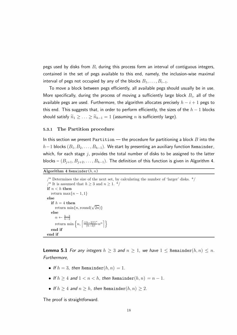
blocks – (Bj+1, Bj+2, . . . , Bh−1). The definition of this function is given in Algorithm 4.
Algorithm 4 Remainder(h, n)
/* Determines the size of the next set, by calculating the number of ‘larger’ disks. *//* It is assumed that h ≥ 3 and n ≥ 1. */if n < h thenreturn max{n− 1, 1}
elseif h = 4 thenreturn min{n, round(
√2n)}
elseα← h−3
h−2
return min{n,⌈((h−2)!)α
(h−3)! nα⌉}
end ifend if
Lemma 5.1 For any integers h ≥ 3 and n ≥ 1, we have 1 ≤ Remainder(h, n) ≤ n.
Furthermore,
• If h = 3, then Remainder(h, n) = 1.
• If h ≥ 4 and 1 < n < h, then Remainder(h, n) = n− 1.
• If h ≥ 4 and n ≥ h, then Remainder(h, n) ≥ 2.
The proof is straightforward.
18
Algorithm 5 Partition(h,B)
/* Returns a partition of the n disks into h− 1 blocks of consecutive disks. *//* It is assumed that h ≥ 2 and B is a non-empty block of disks. */for j ← 1 to h− 2 donj ← Bmax + 1−Bmin
mj ← Remainder(h− j + 1, nj)nj ← nj −mj
Bj ← [Bmin, Bmin + nj − 1] /* if nj = 0, then Bj = ∅ */B ← B −Bj
end for/* B is now a singleton, so that Bh−1 = {Bmax} */Bh−1 ← B
return (B1, . . . , Bh−1)
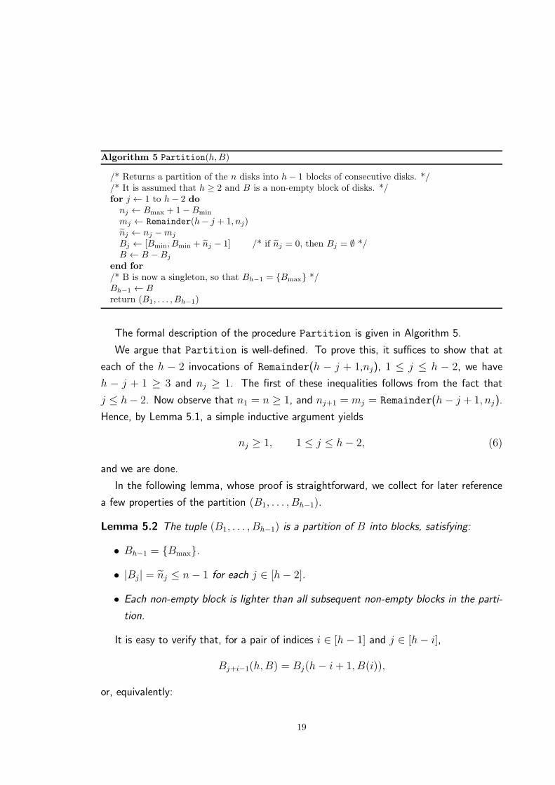
The formal description of the procedure Partition is given in Algorithm 5.
We argue that Partition is well-defined. To prove this, it suffices to show that at
each of the h − 2 invocations of Remainder(h − j + 1,nj), 1 ≤ j ≤ h − 2, we have
h − j + 1 ≥ 3 and nj ≥ 1. The first of these inequalities follows from the fact that
j ≤ h− 2. Now observe that n1 = n ≥ 1, and nj+1 = mj = Remainder(h− j + 1, nj).
Hence, by Lemma 5.1, a simple inductive argument yields
nj ≥ 1, 1 ≤ j ≤ h− 2, (6)
and we are done.
In the following lemma, whose proof is straightforward, we collect for later reference
a few properties of the partition (B1, . . . , Bh−1).
Lemma 5.2 The tuple (B1, . . . , Bh−1) is a partition of B into blocks, satisfying:
• Bh−1 = {Bmax}.
• |Bj| = nj ≤ n− 1 for each j ∈ [h− 2].
• Each non-empty block is lighter than all subsequent non-empty blocks in the parti-
tion.
It is easy to verify that, for a pair of indices i ∈ [h− 1] and j ∈ [h− i],
Bj+i−1(h,B) = Bj(h− i+ 1, B(i)),
or, equivalently:
19
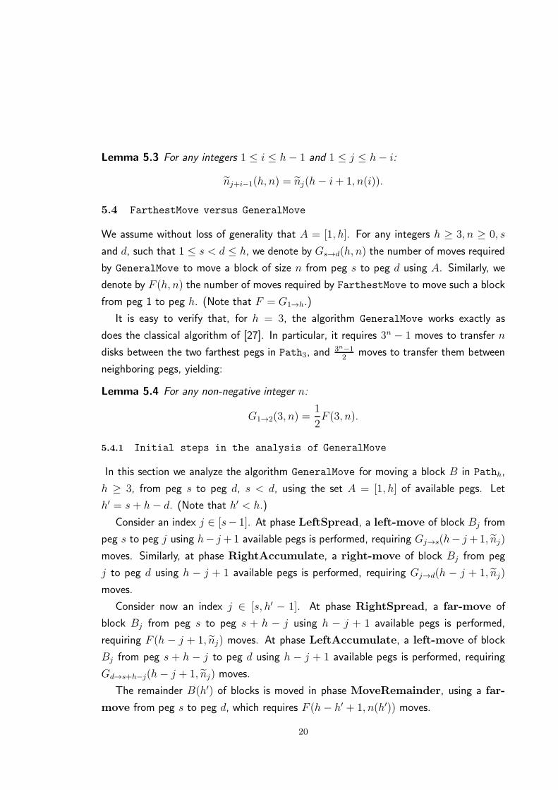
Lemma 5.3 For any integers 1 ≤ i ≤ h− 1 and 1 ≤ j ≤ h− i:
nj+i−1(h, n) = nj(h− i+ 1, n(i)).
5.4 FarthestMove versus GeneralMove
We assume without loss of generality that A = [1, h]. For any integers h ≥ 3, n ≥ 0, s
and d, such that 1 ≤ s < d ≤ h, we denote by Gs→d(h, n) the number of moves required
by GeneralMove to move a block of size n from peg s to peg d using A. Similarly, we
denote by F (h, n) the number of moves required by FarthestMove to move such a block
from peg 1 to peg h. (Note that F = G1→h.)
It is easy to verify that, for h = 3, the algorithm GeneralMove works exactly as
does the classical algorithm of [27]. In particular, it requires 3n − 1 moves to transfer n
disks between the two farthest pegs in Path3, and3n−12
moves to transfer them between
neighboring pegs, yielding:
Lemma 5.4 For any non-negative integer n:
G1→2(3, n) =1
2F (3, n).
5.4.1 Initial steps in the analysis of GeneralMove
In this section we analyze the algorithm GeneralMove for moving a block B in Pathh,
h ≥ 3, from peg s to peg d, s < d, using the set A = [1, h] of available pegs. Let
h′ = s+ h− d. (Note that h′ < h.)
Consider an index j ∈ [s− 1]. At phase LeftSpread, a left-move of block Bj from
peg s to peg j using h− j+1 available pegs is performed, requiring Gj→s(h− j+1, nj)
moves. Similarly, at phase RightAccumulate, a right-move of block Bj from peg
j to peg d using h − j + 1 available pegs is performed, requiring Gj→d(h − j + 1, nj)
moves.
Consider now an index j ∈ [s, h′ − 1]. At phase RightSpread, a far-move of
block Bj from peg s to peg s + h − j using h − j + 1 available pegs is performed,
requiring F (h − j + 1, nj) moves. At phase LeftAccumulate, a left-move of block
Bj from peg s + h − j to peg d using h − j + 1 available pegs is performed, requiring
Gd→s+h−j(h− j + 1, nj) moves.
The remainder B(h′) of blocks is moved in phase MoveRemainder, using a far-
move from peg s to peg d, which requires F (h− h′ + 1, n(h′)) moves.
20
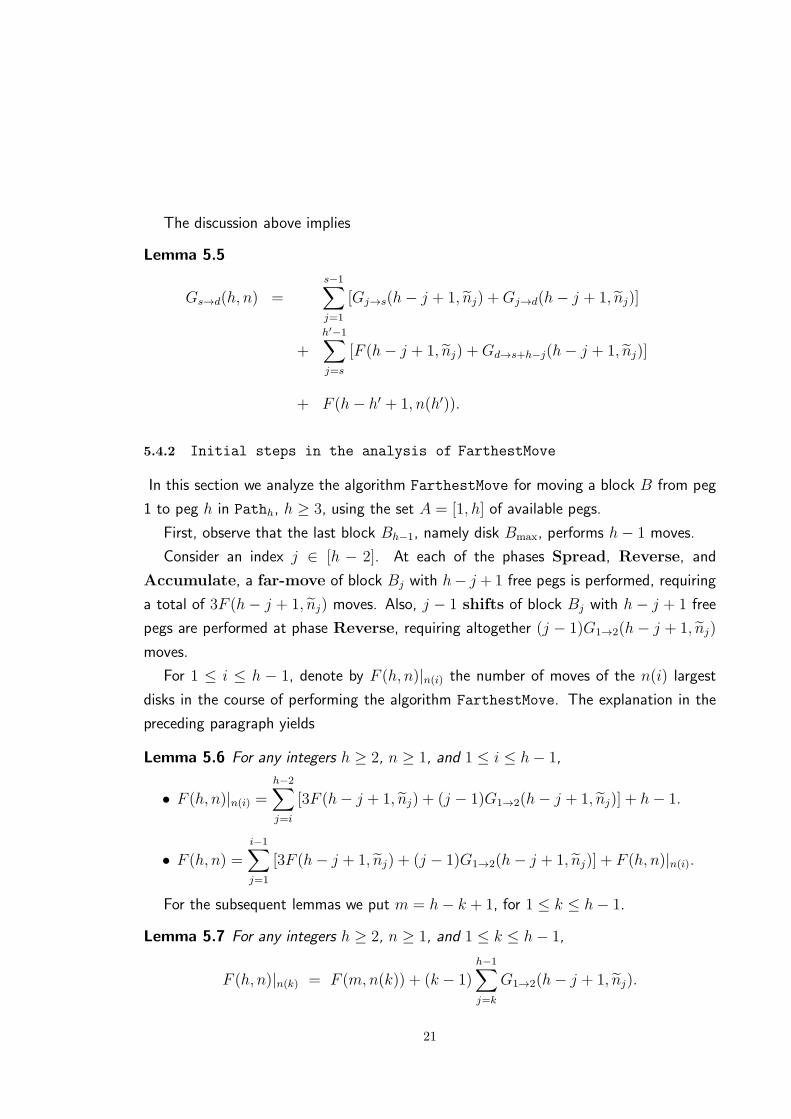
The discussion above implies
Lemma 5.5
Gs→d(h, n) =
s−1∑
j=1
[Gj→s(h− j + 1, nj) +Gj→d(h− j + 1, nj)]
+
h′−1∑
j=s
[F (h− j + 1, nj) +Gd→s+h−j(h− j + 1, nj)]
+ F (h− h′ + 1, n(h′)).
5.4.2 Initial steps in the analysis of FarthestMove
In this section we analyze the algorithm FarthestMove for moving a block B from peg
1 to peg h in Pathh, h ≥ 3, using the set A = [1, h] of available pegs.
First, observe that the last block Bh−1, namely disk Bmax, performs h− 1 moves.
Consider an index j ∈ [h − 2]. At each of the phases Spread, Reverse, and
Accumulate, a far-move of block Bj with h− j +1 free pegs is performed, requiring
a total of 3F (h− j + 1, nj) moves. Also, j − 1 shifts of block Bj with h− j + 1 free
pegs are performed at phase Reverse, requiring altogether (j − 1)G1→2(h− j + 1, nj)
moves.
For 1 ≤ i ≤ h − 1, denote by F (h, n)|n(i) the number of moves of the n(i) largest
disks in the course of performing the algorithm FarthestMove. The explanation in the
preceding paragraph yields
Lemma 5.6 For any integers h ≥ 2, n ≥ 1, and 1 ≤ i ≤ h− 1,
• F (h, n)|n(i) =h−2∑
j=i
[3F (h− j + 1, nj) + (j − 1)G1→2(h− j + 1, nj)] + h− 1.
• F (h, n) =
i−1∑
j=1
[3F (h− j + 1, nj) + (j − 1)G1→2(h− j + 1, nj)] + F (h, n)|n(i).
For the subsequent lemmas we put m = h− k + 1, for 1 ≤ k ≤ h− 1.
Lemma 5.7 For any integers h ≥ 2, n ≥ 1, and 1 ≤ k ≤ h− 1,
F (h, n)|n(k) = F (m,n(k)) + (k − 1)h−1∑
j=k
G1→2(h− j + 1, nj).
21
Proof: By Lemma 5.6 in the particular case i = 1,
F (m,n(k)) =
m−2∑
j=1
[3F (m− j + 1, nj(m,n(k)))
+ (j − 1)G1→2(m− j + 1, nj(m,n(k)))] + h− k.
By Lemma 5.3, we obtain
F (m,n(k)) =m−2∑
j=1
[3F (m− j + 1, nj+k−1)
+ (j − 1)G1→2(m− j + 1, nj+k−1)] + h− k
=
h−2∑
j=k
[3F (h− j + 1, nj) + (j − k)G1→2(h− j + 1, nj)] + h− k.
(7)
Observe that G1→2(2, nh−1) = 1. Thus, by Lemma 5.6, the right-hand side of (7)
reduces to
F (h, n)|n(k) − (k − 1)
h−1∑
j=k
G1→2(h− j + 1, nj),
and we are done.
Lemma 5.6 and Lemma 5.7 imply
Corollary 5.8 For any integers h ≥ 2, n ≥ 1, and 1 ≤ k ≤ h− 1,
F (h, n) =
k−1∑
j=1
[3F (h− j + 1, nj) + (j − 1)G1→2(h− j + 1, nj)]
+ F (m,n(k)) + (k − 1)h−1∑
j=k
G1→2(h− j + 1, nj).
5.4.3 Moving from one End to the Other is the most Costly
The following statement shows that GeneralMove requires the maximal number of moves
when the source and destination pegs are at the extreme ends of the set A.
Proposition 5.9 For integers h ≥ 3, n ≥ 1, s, d, such that 1≤s<d≤h and d−s+1 < h,
Gs→d(h, n) < F (h, n).
22
Proof: Denote h′′ = h−h′+1. The proof is by induction on n, for all values of h ≥ 3.
For n = 1, we have nj = 0 for each 1 ≤ j ≤ h− 2. Hence by Lemma 5.5,
Gs→d(h, 1) = F (h′′, 1) = h′′ − 1 = d− s < h− 1 = F (h, 1).
We assume that the statement holds for less than n disks and all h ≥ 3, and prove it for
n disks and all h ≥ 3. Observe that
1 < s+ h− d = h′ ≤ h− 1.
By Lemma 5.2, for each 1 ≤ j ≤ h′ − 1, we have nj < n. Thus, by Lemma 5.5 and the
induction hypothesis,
Gs→d(h, n) ≤h′−1∑
j=1
2F (h− j + 1, nj) + F (h′′, n(h′))
<
h′−1∑
j=1
2F (h− j + 1, nj) + F (h′′, n(h′)) + (h′ − 1).
Since h′ ≤ h− 1 and nh−1 = 1:
h−1∑
j=h′
G1→2(h− j + 1, nj) ≥ G1→2(2, nh−1) = 1.
Thus by Corollary 5.8,
F (h, n) ≥h′−1∑
j=1
3F (h− j + 1, nj) + F (h′′, n(h′)) + (h′ − 1)
h−1∑
j=h′
G1→2(h− j + 1, nj)
≥h′−1∑
j=1
2F (h− j + 1, nj) + F (h′′, n(h′)) + (h′ − 1)
> Gs→d(h, n).
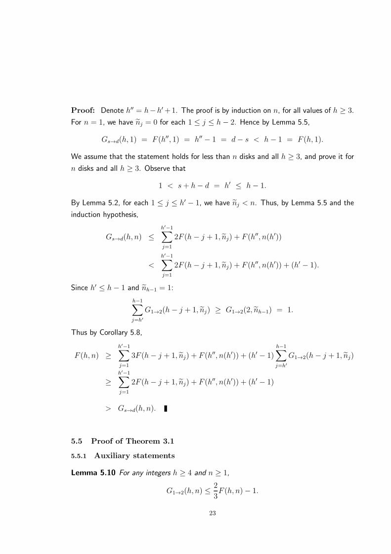
5.5 Proof of Theorem 3.1
5.5.1 Auxiliary statements
Lemma 5.10 For any integers h ≥ 4 and n ≥ 1,
G1→2(h, n) ≤2
3F (h, n)− 1.
23
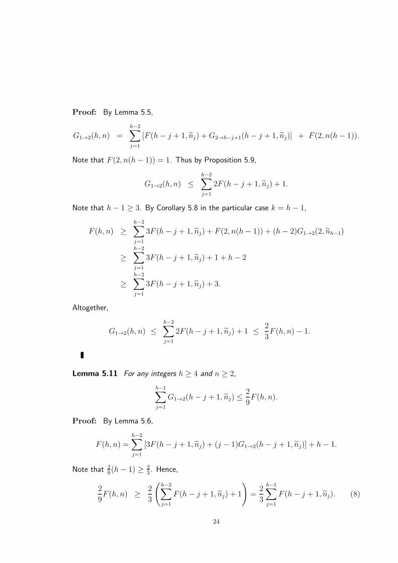
Proof: By Lemma 5.5,
G1→2(h, n) =h−2∑
j=1
[F (h− j + 1, nj) +G2→h−j+1(h− j + 1, nj)] + F (2, n(h− 1)).
Note that F (2, n(h− 1)) = 1. Thus by Proposition 5.9,
G1→2(h, n) ≤h−2∑
j=1
2F (h− j + 1, nj) + 1.
Note that h− 1 ≥ 3. By Corollary 5.8 in the particular case k = h− 1,
F (h, n) ≥h−2∑
j=1
3F (h− j + 1, nj) + F (2, n(h− 1)) + (h− 2)G1→2(2, nh−1)
≥h−2∑
j=1
3F (h− j + 1, nj) + 1 + h− 2
≥h−2∑
j=1
3F (h− j + 1, nj) + 3.
Altogether,
G1→2(h, n) ≤h−2∑
j=1
2F (h− j + 1, nj) + 1 ≤ 2
3F (h, n)− 1.
Lemma 5.11 For any integers h ≥ 4 and n ≥ 2,
h−1∑
j=1
G1→2(h− j + 1, nj) ≤2
9F (h, n).
Proof: By Lemma 5.6,
F (h, n) =h−2∑
j=1
[3F (h− j + 1, nj) + (j − 1)G1→2(h− j + 1, nj)] + h− 1.
Note that 29(h− 1) ≥ 2
3. Hence,
2
9F (h, n) ≥ 2
3
(h−2∑
j=1
F (h− j + 1, nj) + 1
)=
2
3
h−1∑
j=1
F (h− j + 1, nj). (8)
24
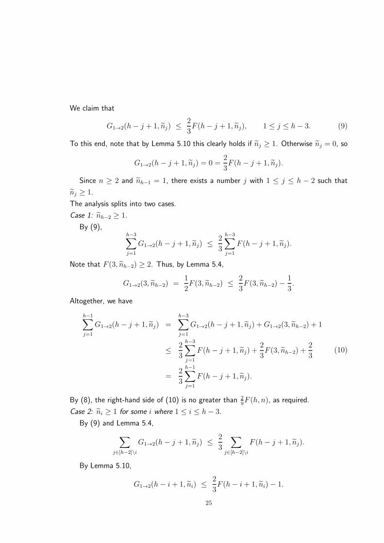
We claim that
G1→2(h− j + 1, nj) ≤2
3F (h− j + 1, nj), 1 ≤ j ≤ h− 3. (9)
To this end, note that by Lemma 5.10 this clearly holds if nj ≥ 1. Otherwise nj = 0, so
G1→2(h− j + 1, nj) = 0 =2
3F (h− j + 1, nj).
Since n ≥ 2 and nh−1 = 1, there exists a number j with 1 ≤ j ≤ h − 2 such that
nj ≥ 1.
The analysis splits into two cases.
Case 1: nh−2 ≥ 1.
By (9),h−3∑
j=1
G1→2(h− j + 1, nj) ≤2
3
h−3∑
j=1
F (h− j + 1, nj).
Note that F (3, nh−2) ≥ 2. Thus, by Lemma 5.4,
G1→2(3, nh−2) =1
2F (3, nh−2) ≤
2
3F (3, nh−2)−
1
3.
Altogether, we have
h−1∑
j=1
G1→2(h− j + 1, nj) =h−3∑
j=1
G1→2(h− j + 1, nj) +G1→2(3, nh−2) + 1
≤ 2
3
h−3∑
j=1
F (h− j + 1, nj) +2
3F (3, nh−2) +
2
3
=2
3
h−1∑
j=1
F (h− j + 1, nj).
(10)
By (8), the right-hand side of (10) is no greater than 29F (h, n), as required.
Case 2: ni ≥ 1 for some i where 1 ≤ i ≤ h− 3.
By (9) and Lemma 5.4,
∑
j∈[h−2]\iG1→2(h− j + 1, nj) ≤
2
3
∑
j∈[h−2]\iF (h− j + 1, nj).
By Lemma 5.10,
G1→2(h− i+ 1, ni) ≤2
3F (h− i+ 1, ni)− 1.
25
Altogether, we have
h−1∑
j=1
G1→2(h− j + 1, nj) =∑
j∈[h−2]\{i}G1→2(h− j + 1, nj) +G1→2(h− i+ 1, ni) + 1
≤ 2
3
h−2∑
j=1
F (h− j + 1, nj).
(11)
By (8), the right-hand side of (11) is strictly less than 29F (h, n), and we are done.
Lemma 5.12 For any integers h ≥ 5 and n ≥ h,
F (h, n) ≤ 3F (h, n1) +11
9F (h− 1, n− n1).
Proof: By Corollary 5.8 in the particular case k = 2,
F (h, n) = 3F (h, n1) + F (h− 1, n− n1) +
h−1∑
j=2
G1→2(h− j + 1, nj).
We have n ≥ h ≥ 5. Thus, h− 1 ≥ 4, and by Lemma 5.1 we have n− n1 ≥ 2. Applying
Lemma 5.11 with h− 1 and n− n1 instead of h and n, respectively, we get
h−2∑
j=1
G1→2(h− j, nj(h− 1, n− n1)) ≤2
9F (h− 1, n− n1). (12)
By Lemma 5.3 in the particular case i = 2, for each 1 ≤ j ≤ h− 2,
nj+1(h, n) = nj(h− 1, n− n1).
Consequently,
h−1∑
j=2
G1→2(h− j + 1, nj) =h−2∑
j=1
G1→2(h− j, nj(h− 1, n− n1)) ≤2
9F (h− 1, n− n1),
which provides the required result.
Lemma 5.13 For any integers h ≥ 5 and 1 ≤ n < h,
F (h, n) ≤ U(h, n) = Ch · nαh · 3θh·n1
h−2< U(h, n),
where θh and αh are as in Theorem 3.1, and Ch = h−2θh
.
26
Proof: First note that U(h, n) < U(h, n), so it remains to prove that F (h, n) ≤U(h, n). Since h ≥ 5 and n < h, Lemmas 5.1 and 5.2 imply that ni = 1 for each
i ∈ [n− 1] ∪ {h− 1}. Thus by Lemma 5.6,
F (h, n) =h−2∑
j=1
[3F (h− j + 1, nj) + (j − 1)G1→2(h− j + 1, nj)] + h− 1
=
n−1∑
j=1
[3F (h− j + 1, 1) + (j − 1)G1→2(h− j + 1, 1)] + h− 1
=
n−1∑
j=1
3(h− j) + (j − 1) + h− 1 = n(3h− n)− 2h.
It is easy to verify that for h ≥ 5 and n < h,
n(3h− n)− 2h ≤ 3n(h− 2).
Note that θhn1
h−2 ≥ 1 for h ≥ 3 and n ≥ 1. For x ≥ 1, we have x ≤ 3x−1. Therefore,
3θhn1
h−2 ≤ 3θhn1
h−2,
and consequently,
3n(h− 2) ≤ h− 2
θhnαh · 3θhn
1h−2
.
Altogether,
F (h, n) ≤ 3n(h− 2) ≤ h− 2
θhnαh · 3θh·n
1h−2
= U(h, n).
5.5.2 Conclusion of the Proof
The proof is by double induction on h ≥ 3 and n.
For h = 3, the algorithm works exactly as does the algorithm of [27] for the 3-in-a-row
graph. Therefore, the number F (3, n) of moves required by this algorithm for n disks is
3n− 1. The substitution h = 3 in the upper bound U(h, n) suggested by the proposition
yields:
U(3, n) = Chnαh · 3θhn
1/ 1h−2
= 1 · n0 · 31·n = 3n > F (3, n).
For h = 4, the algorithm works exactly as does the algorithm FourMove of Section 4.2 for
moving n disks between the two farthest pegs in Path4. Therefore, as shown in Section
27
4.2, F (4, n) is bounded above by 1.6√n · 3
√2n. The substitution h = 4 in the upper
bound U(h, n) suggested by the proposition yields:
U(4, n) = Chnαh · 3θhn
1h−2
= c√2n · 3
√2n > 1.6
√n · 3
√2n ≥ F (4, n).
For h ≥ 5 and n < h, Lemma 5.13 implies that F (h, n) < U(h, n).
We assume that for arbitrary fixed h ≥ 5 and n ≥ h, F (h′, n′) < U(h′, n′) holds for
all (h′, n′) with either h′ < h or both h′ = h and n′ < n, and prove it for (h, n).
Let m = m1 = Remainder(h, n). Then n1 = n−m. By Lemma 5.12,
F (h, n) ≤ 3F (h, n−m) +11
9F (h− 1, m).
The analysis splits into two cases.
Case 1: n ≤ (h−2)h−2
(h−2)!.
In this case, we have
n ≤ ((h− 2)!)αh
(h− 3)!nαh , (13)
and so,
m = Remainder(h, n) = min
{n,
⌈((h− 2)!)αh
(h− 3)!nαh
⌉}= n.
It follows that F (h, n) ≤ 119F (h− 1, n). By the induction hypothesis,
F (h, n) <11
9U(h− 1, n) =
11
9Ch−1 · nαh−1 · 3θh−1·n
1h−3
. (14)
By (13), we have
θh−1 · n1
h−3 ≤ θh−1
(((h− 2)!)αh
(h− 3)!nαh
) 1h−3
= θh−1
(θh−3h
θh−3h−1
nh−3h−2
) 1h−3
= θh · n1
h−2 . (15)
Substituting (15) in (14), we obtain
F (h, n) <11
9Ch−1 · nαh−1 · 3θh·n
1h−2
. (16)
It is easy to verify that 119Ch−1 < Ch and αh−1 < αh. Thus we find that:
F (h, n) < Ch · nαh · 3θh·n1
h−2.
Case 2: n >(h−2)h−2
(h−2)!.
28
In this case, we have
n >((h− 2)!)αh
(h− 3)!nαh ,
and so,
m=Remainder(h, n)=min
{n,
⌈((h− 2)!)αh
(h− 3)!nαh
⌉}=
⌈((h− 2)!)αh
(h− 3)!nαh
⌉≤n.
By the induction hypothesis,
F (h, n) < 3Ch(n−m)αh3θh·(n−m)1
h−2+
11
9Ch−1 ·mαh−1 · 3θh−1·m
1h−3
. (17)
Observe that
(n−m)αh = nαh
(1− m
n
)αh
< nαh
(1− αhm
n
). (18)
Similarly, we have
θh(n−m)1
h−2 = θhn1
h−2
(1−m
n
) 1h−2
<θhn1
h−2
(1− θh−3
h · nh−3h−2
(h− 2)nθh−3h−1
)=θhn
1h−2−1 (19)
and
θh−1 ·m1
h−3 ≤ θh−1
(θh−3h
θh−3h−1
· nh−3h−2 + 1
) 1h−3
= θhn1
h−2
(1 +
θh−3h−1
θh−3h
n−h−3h−2
) 1h−3
< θhn1
h−2 +(h− 3)! · θ2h(h−3)(h−2)!n
−h−4h−2 = θhn
1h−2 +
θ2h(h−3)(h−2)n
−h−4h−2 .
It is easy to verify that ϑ(h, n) =θ2h
(h−3)(h−2)n−h−4
h−2 is monotone decreasing with h and n
in the range n ≥ h ≥ 5. Hence for n ≥ h ≥ 5, we have
ϑ(h, n) ≤ ϑ(5, 5) =
(1
30
)1/3
.
Put c∗ =(
130
)1/3. Now
θh−1 ·m1
h−3 < θh · n1
h−2 + c∗. (20)
Substituting (18), (19) and (20) in (17), we obtain
F (h, n) < 3Chnαh(1− αh·m
n
)3θh·n
1h−2−1 + 11
9Ch−1 ·mαh−1 · 3θh·n
1h−2 +c∗
= Chnαh(1− αh·m
n
)3θh·n
1h−2
+ 1193c
∗Ch−1 ·mαh−1 · 3θh·n
1h−2
=(Chn
αh − Ch·nαh ·αh·mn
+ δ · Ch−1 ·mαh−1)3θh·n
1h−2
.
(21)
29
The second and third terms on the right-hand side of (21) may be omitted since:
δCh−1 ·mαh−1 − Ch·nαh ·αh·mn
= mαh−1
(δ(h−3)δh−4
θh−1− (h−2)δh−3
n·θh · nh−3h−2 · h−3
h−2·m 1
h−3
)
= mαh−1(h− 3)δh−3
(1
θh−1− n
−1h−2 ·m
1h−3
θh
)
≤ mαh−1(h−3)δh−3
(1
θh−1− n
−1h−2
θh
(θh−3h
θh−3h−1
· nh−3h−2
) 1h−3
)
= 0.
Thus we conclude that:
F (h, n) < Chnαh · 3θh·n
1h−2
.
References
[1] J.-P. Allouche, D. Astoorian, J. Randall, and J. Shallit. Morphisms, squarefree
strings, and the Tower of Hanoi puzzle. Amer. Math. Monthly, 101:651–658, 1994.
[2] J.-P. Allouche and A. Sapir. Restricted Towers of Hanoi and morphisms. LNCS,
3572:1–10, 2005.
[3] M. D. Atkinson. The cyclic Towers of Hanoi. Inform. Process. Lett., 13:118–119,
1981.
[4] D. Azriel and D. Berend. On a question of Leiss regarding the Hanoi Tower problem.
Theoretical Computer Science, 369:377–383, 2006.
[5] D. Azriel, N. Solomon, and S. Solomon. On an infinite family of solvable Hanoi
graphs. Trans. on Algorithms, 5(1), 2008.
[6] D. Berend and A. Sapir. The Cyclic multi-peg Tower of Hanoi. Trans. on Algorithms,
2(3):297–317, 2006.
[7] D. Berend and A. Sapir. The diameter of Hanoi graphs. Inform. Process. Lett.,
98:79–85, 2006.
30
[8] X. Chen and J. Shen. On the Frame-Stewart conjecture about the Towers of Hanoi.
SIAM J. on Computing, 33(3):584–589, 2004.
[9] Y. Dinitz and S. Solomon. Optimal algorithms for Tower of Hanoi problems with
relaxed placement rules. Proc. of ISSAC06, pages 36–47, 2006.
[10] Y. Dinitz and S. Solomon. On Optimal solutions for the Bottleneck Tower of Hanoi
problem. Proc. of SOFSEM07, pages 248–259, 2007.
[11] Y. Dinitz and S. Solomon. Optimality of an algorithm solving the Bottleneck Tower
of Hanoi problem. Trans. on Algorithms, 4(3):1–9, 2008.
[12] H. E. Dudeney. “The Canterbury Puzzles (and Other Curious Problems)”. E. P.
Dutton, New York, 1908.
[13] M. C. Er. The Cyclic Towers of Hanoi: a representation approach. Comput. J.,
27(2):171–175, 1984.
[14] M. C. Er. The complexity of the generalised Cyclic Towers of Hanoi. J. Algorithms,
6:351–358, 1985.
[15] J. S. Frame. Solution to advanced problem 3918. Amer. Math. Monthly, 48:216–217,
1941.
[16] A. M. Hinz. Pascal’s triangle and the Tower of Hanoi. Amer. Math. Monthly,
99:538–544, 1992.
[17] S. Klavzar, U. Milutinovic, and C. Petr. On the Frame-Stewart algorithm for the
multi-peg Tower of Hanoi problem. Discrete Applied Math., 120(1-3):141–157, 2002.
[18] S. Klavzar, U. Milutinovic, and C. Petr. Hanoi graphs and some classical numbers.
Expo. Math., 23(4):371–378, 2005.
[19] E. L. Leiss. Finite Hanoi problems: how many discs can be handled? Congr. Numer.,
44(1):221–229, 1984.
[20] E. Lucas. “Recreations Mathematiques”, volume III. Gauthier-Villars, Paris, 1893.
[21] W. F. Lunnon and P. K. Stockmeyer. New Variations on the Tower of Hanoi.
[22] S. Minsker. The Little Towers of Antwerpen problem. Inform. Process. Lett.,
94(5):197–201, 2005.
31
[23] S. Minsker. The Linear Twin Towers of Hanoi problem. ACM SIGCSE Bull.,
39(4):37–40, 2007.
[24] S. Minsker. Another brief recursion excursion to Hanoi. ACM SIGCSE Bull.,
40(4):35–37, 2008.
[25] S. Minsker. The classical/linear Hanoi hybrid problem: regular configurations. ACM
SIGCSE Bull., 41(4):57–61, 2009.
[26] A. Sapir. The Tower of Hanoi with forbidden moves. Comput. J., 47(1):20–24, 2004.
[27] R. S. Scorer, P. M. Grundy, and C. A. B. Smith. Some binary games. Math. Gazette,
280:96–103, 1944.
[28] B. M. Stewart. Advanced problem 3918. Amer. Math. Monthly, 46:363, 1939.
[29] B. M. Stewart. Solution to advanced problem 3918. Amer. Math. Monthly, 48:217–
219, 1941.
[30] P. K. Stockmeyer. Variations on the Four-Post Tower of Hanoi puzzle. Congr.
Numer., 102:3–12, 1994.
[31] P. K. Stockmeyer. The average distance between nodes in the Cyclic Tower of Hanoi
digraph. Graph Theory, Combinatorics, Algorithms, and Applications, 1996.
[32] M. Szegedy. In how many steps the k peg version of the Towers of Hanoi game can
be solved? Lect. Notes in Comput. Sci., 1563:356–361, 1999.
32


![Matrix Representation of Hanoi Graphs · Graph and Finite Automata. [2] S. Klavzar and U. Milutinovic, Graphs S(n,k) and a variant of the Tower of Hanoi Problem, Czechoslovak Math](https://img.pdfslide.us/doc/110x75/5f925f6a92fe24378f38656e/matrix-representation-of-hanoi-graphs-graph-and-finite-automata-2-s-klavzar.jpg)