Embed Size (px)
Citation preview
Reasoning and Decision in Probabilistic Graphical models – A Unified Approach
Qiang LiuThesis Defense
Dissertation Committee : Alexander Ihler (chair)Rina DechterPadhraic Symth
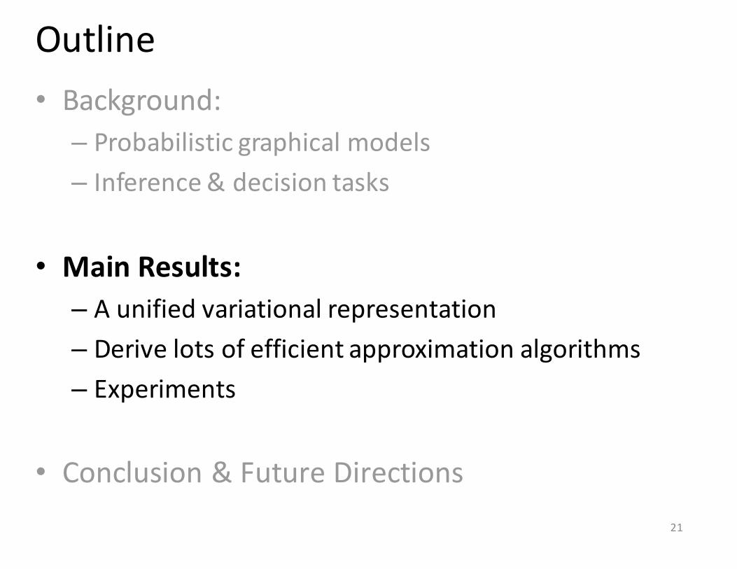
Outline• Background:– Probabilistic graphical models– Inference & decision tasks
• Main Results:– A unified variational representation– Derive lots of efficient approximation algorithms– Experiments
• Conclusion & Future Directions2
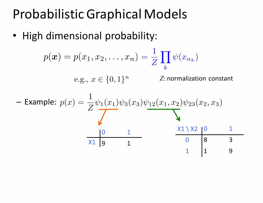
Probabilistic Graphical Models• High dimensional probability:
=1
Z
Y
k
(x↵k)
– Example:
0 10 8 31 1 9
X1 \ X20 19 1X1
p(x) =1
Z
1(x1) 3(x3) 12(x1, x2) 23(x2, x3)
p(x) = p(x1, x2, . . . , xn)
Discrete: e.g., x 2 {0, 1}n Z: normalization constant
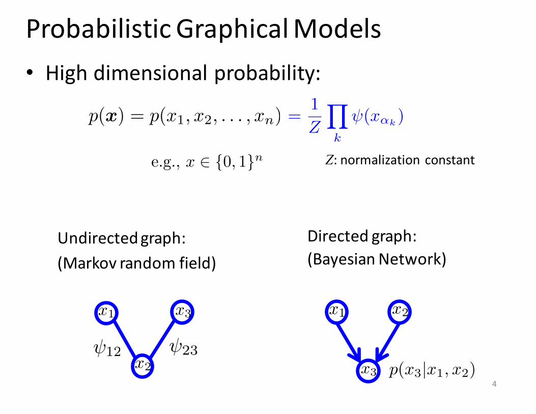
Probabilistic Graphical Models
x1 x2
x3
Directed graph:(Bayesian Network)
p(x3|x1, x2)
• High dimensional probability:
=1
Z
Y
k
(x↵k)p(x) = p(x1, x2, . . . , xn)
Discrete: e.g., x 2 {0, 1}n Z: normalization constant
4
Undirected graph: (Markov random field)
x1
x2
x3
12 23
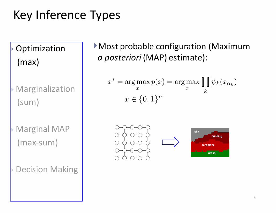
‣Most probable configuration (Maximum a posteriori (MAP) estimate):
Key Inference Types
x
⇤= argmax
x
p(x) = argmax
x
Y
k
k
(x
↵k)
x 2 {0, 1}n
‣Optimization(max)
‣Marginalization(sum)
‣Marginal MAP(max-‐sum)
‣Decision Making
5
‣Optimization(max)
‣Marginalization(sum)
‣Marginal MAP(max-‐sum)
‣Decision Making
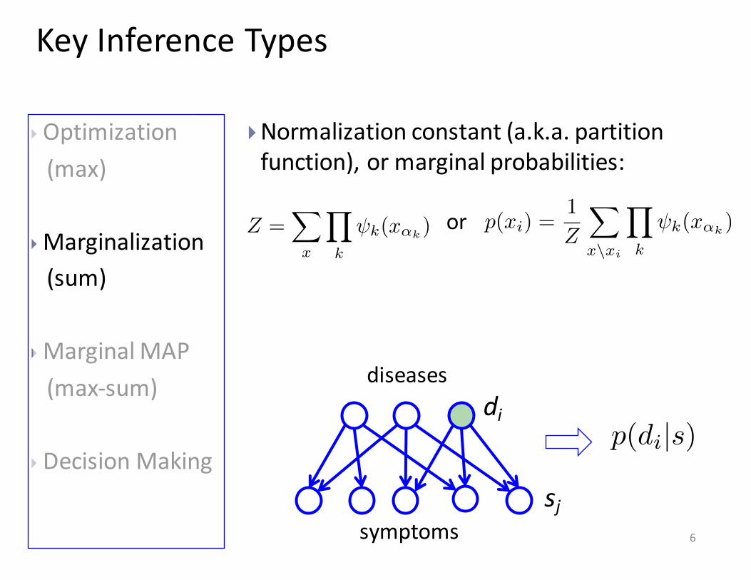
}Normalization constant (a.k.a. partition function), or marginal probabilities:
Key Inference Types
diseases
symptoms
di
sj
p(di|s)
Z =X
x
Y
k
k
(x↵k) p(x
i
) =1
Z
X
x\xi
Y
k
k
(x↵k)or
6
}Maximize marginal probability, or expected objective w.r.t. “latent variables”:
Key Inference Types
}Latent variables: }Missing labels:
Black: missing labels
‣Optimization(max)
‣Marginalization(sum)
‣Marginal MAP(max-‐sum)
‣Decision Making
x = [xA, xB ]
x
⇤B
= argmax
xB
X
xA
p([x
A
, x
B
]) = argmax
xB
X
xA
Y
k
k
(x
↵k)
7
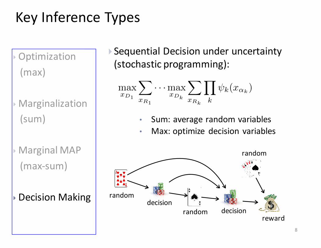
}Sequential Decision under uncertainty (stochastic programming):
Key Inference Types
• Sum: average random variables • Max: optimize decision variables
randomdecision
reward
random
random decision
max
xD1
X
xR1
· · ·max
xDk
X
xRk
Y
k
k
(x
↵k)
‣Optimization(max)
‣Marginalization(sum)
‣Marginal MAP(max-‐sum)
‣Decision Making
8
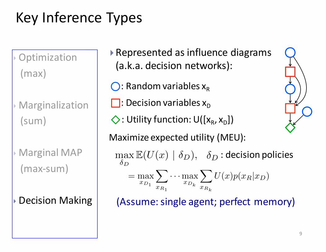
Key Inference Types
}Represented as influence diagrams (a.k.a. decision networks):
: Random variables xR: Decision variables xD: Utility function: U([xR, xD])
(Assume: single agent; perfect memory)
Maximize expected utility (MEU):
= max
xD1
X
xR1
· · ·max
xDk
X
xRk
U(x)p(x
R
|xD
)
‣Optimization(max)
‣Marginalization(sum)
‣Marginal MAP(max-‐sum)
‣Decision Making
9
�Dmax
�DE(U(x) | �D),
: decision policies
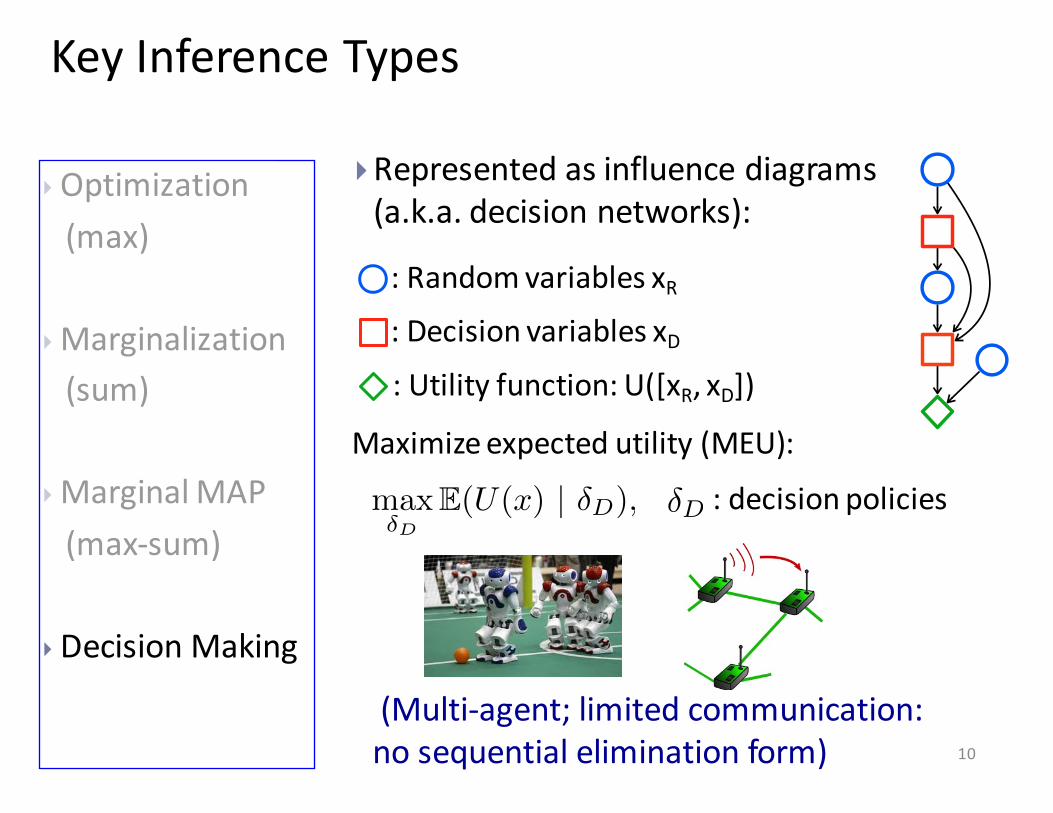
Key Inference Types
}Represented as influence diagrams (a.k.a. decision networks):
: Random variables xR: Decision variables xD: Utility function: U([xR, xD])
Maximize expected utility (MEU):
‣Optimization(max)
‣Marginalization(sum)
‣Marginal MAP(max-‐sum)
‣Decision Making
10
�Dmax
�DE(U(x) | �D),
: decision policies
(Multi-‐agent; limited communication: no sequential elimination form)
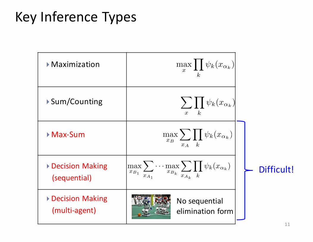
}Sum/Counting
}Maximization
}Max-‐Sum
Key Inference Types
}Decision Making(sequential)
}Decision Making(multi-‐agent)
No sequential elimination form
Difficult!max
xB1
X
xA1
· · ·max
xBk
X
xAk
Y
k
k
(x
↵k)
max
xB
X
xA
Y
k
k
(x
↵k)
X
x
Y
k
k
(x↵k)
max
x
Y
k
k
(x
↵k)
11
Pure sum or max are (relatively) “easy”
=X
x2,x3
3(x3) 23(x2, x3)X
x1
12(x1, x2)
=X
x2,x3
3(x3) 23(x2, x3)m1!2(x2)
=X
x3
3(x3)X
x2
23(x2, x3)m1!2(x2)
=X
x3
3(x3)m2!3(x3)
Z =X
x1,x2,x3
3(x3) 23(x2, x3) 12(x1, x2)x1 x3x2 12
3 23
m1!2 m2!3
• Dynamic programming.
“message passing”
12
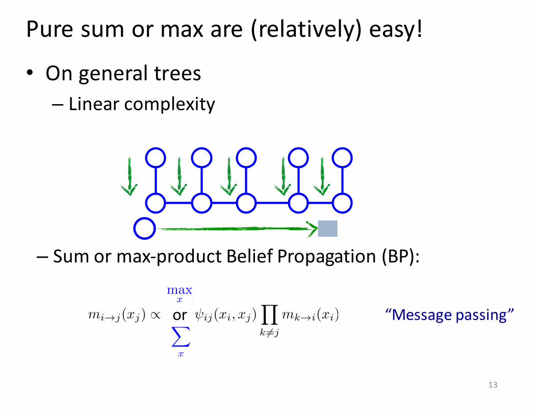
Pure sum or max are (relatively) easy!
m
i!j
(x
j
) /max
xX
x
ij
(x
i
, x
j
)
Y
k 6=j
m
k!i
(x
i
)
• On general trees – Linear complexity
“Message passing”
– Sum or max-‐product Belief Propagation (BP):
m
i!j
(x
j
) /max
xX
x
ij
(x
i
, x
j
)
Y
k 6=j
m
k!i
(x
i
)
m
i!j
(x
j
) /max
xX
x
ij
(x
i
, x
j
)
Y
k 6=j
m
k!i
(x
i
)
or
13
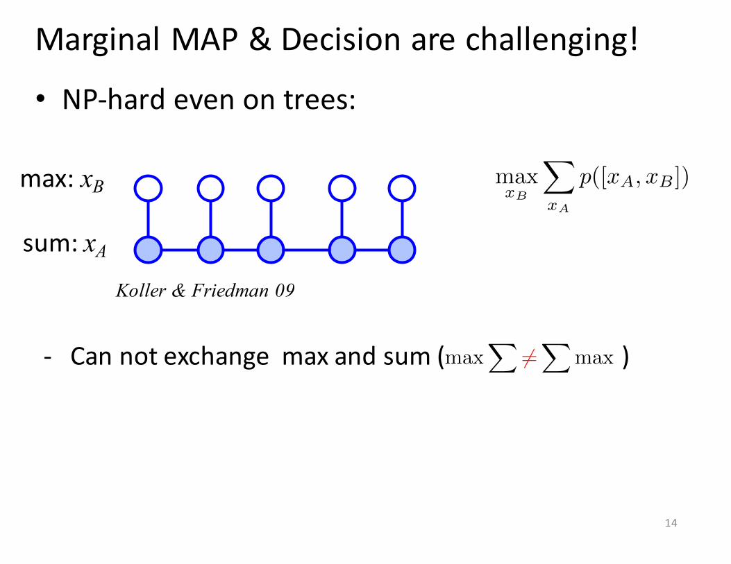
• NP-‐hard even on trees:
Marginal MAP & Decision are challenging!
Koller & Friedman 09
max: xB
sum: xA
max
xB
X
xA
p([x
A
, x
B
])
14
-‐ Can not exchange max and sum ( )max
X6=X
max
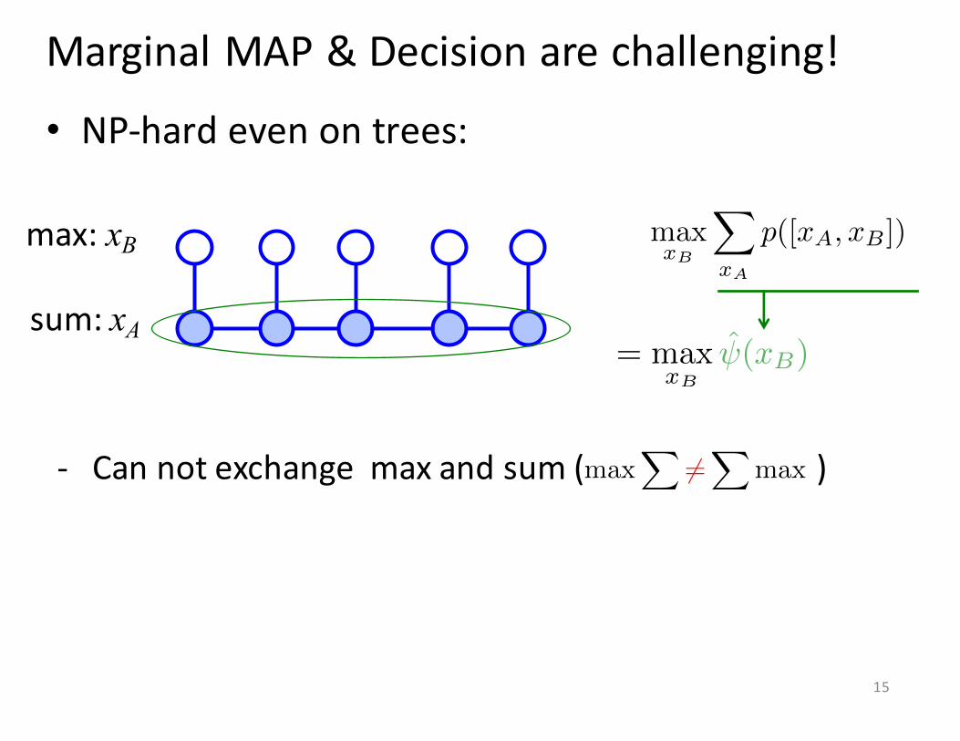
Marginal MAP & Decision are challenging!
• NP-‐hard even on trees:
= max
xB
ˆ
(x
B
)
max: xB
sum: xA
max
xB
X
xA
p([x
A
, x
B
])
15
-‐ Can not exchange max and sum ( )max
X6=X
max
Use Joint Optimization instead?
[x
⇤A
, x
⇤B
] = argmax
x
p([x
A
, x
B
])
16
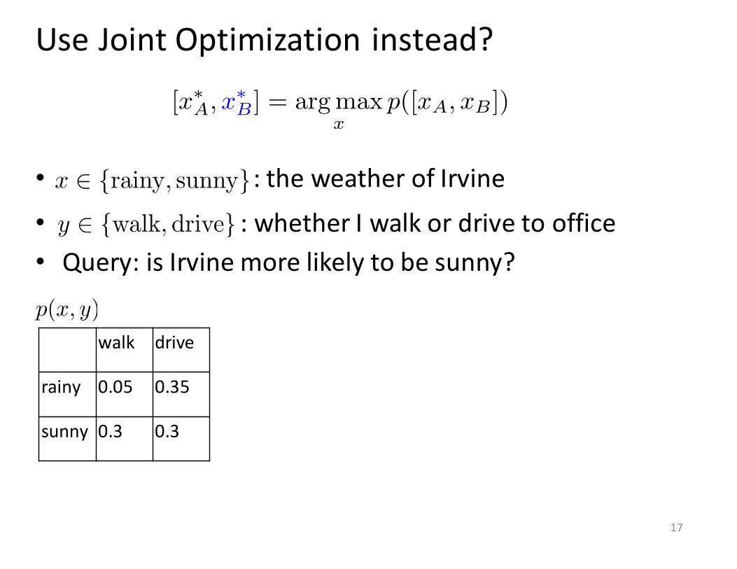
walk drive
rainy 0.05 0.35
sunny 0.3 0.3
Use Joint Optimization instead?
• : the weather of Irvine• : whether I walk or drive to office• Query: is Irvine more likely to be sunny?
[x
⇤A
, x
⇤B
] = argmax
x
p([x
A
, x
B
])
17
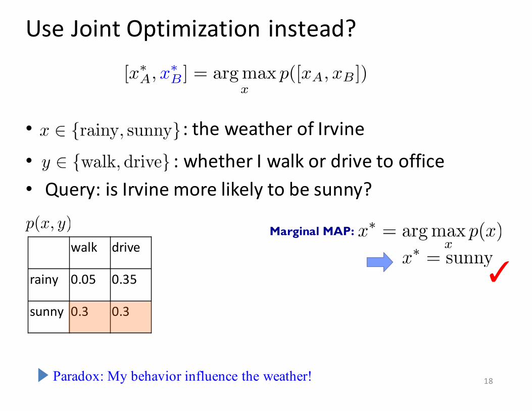
walk drive
rainy 0.05 0.35
sunny 0.3 0.3
Marginal MAP:
✓
Paradox: My behavior influence the weather!
Use Joint Optimization instead?
• : the weather of Irvine• : whether I walk or drive to office• Query: is Irvine more likely to be sunny?
[x
⇤A
, x
⇤B
] = argmax
x
p([x
A
, x
B
])
18
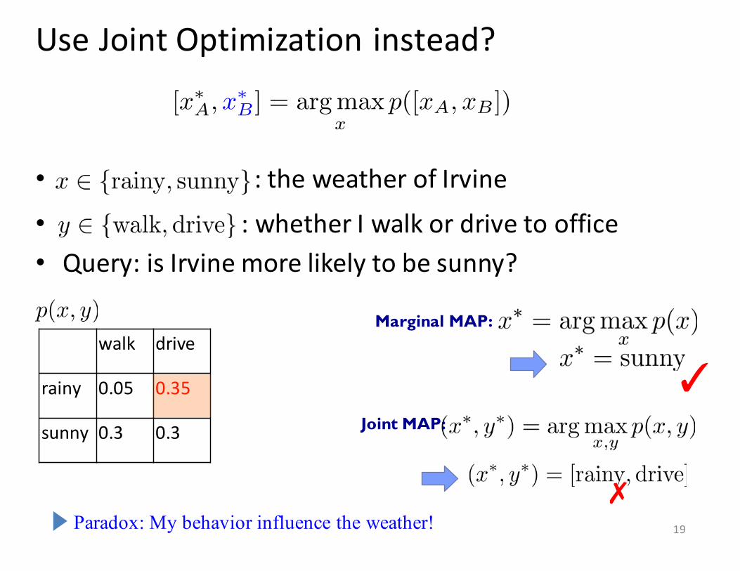
walk drive
rainy 0.05 0.35
sunny 0.3 0.3 Joint MAP:
✗
Marginal MAP:
✓
Use Joint Optimization instead?
• : the weather of Irvine• : whether I walk or drive to office• Query: is Irvine more likely to be sunny?
Paradox: My behavior influence the weather!
[x
⇤A
, x
⇤B
] = argmax
x
p([x
A
, x
B
])
19
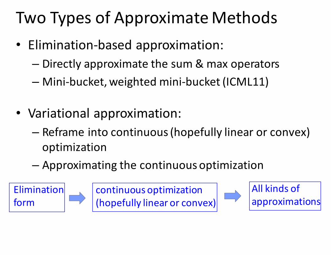
Two Types of Approximate Methods• Elimination-‐based approximation:– Directly approximate the sum & max operators–Mini-‐bucket, weighted mini-‐bucket (ICML11)
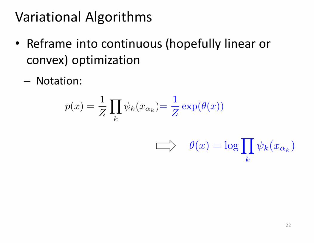
• Variational approximation:– Reframe into continuous (hopefully linear or convex) optimization
– Approximating the continuous optimization
continuous optimization(hopefully linear or convex)
Elimination form
All kinds of approximations
Outline• Background:– Probabilistic graphical models– Inference & decision tasks
• Main Results:– A unified variational representation– Derive lots of efficient approximation algorithms– Experiments
• Conclusion & Future Directions21
Variational Algorithms
• Reframe into continuous (hopefully linear or convex) optimization– Notation:
(Let ✓(x) = log
Y
k
k(x↵k))
p(x) =
1
Z
Y
k
k(x↵k)=
1
Z
exp(✓(x))
22
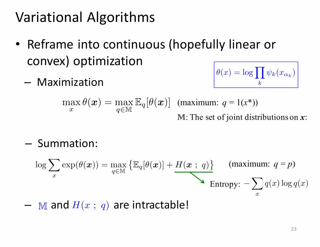
Variational Algorithms
(maximum: q = p)
M: The set of joint distributions on x:
• Reframe into continuous (hopefully linear or convex) optimization– Maximization
– Summation:
log
X
x
exp(✓(x)) = max
q2M
�Eq
[✓(x)] +H(x ; q)
max
x
✓(x) = max
q2MEq
[✓(x)] (maximum: q = 1(x*))
Entropy: �X
x
q(x) log q(x)
– and are intractable!M H(x ; q)
23
(Let ✓(x) = log
Y
k
k(x↵k))
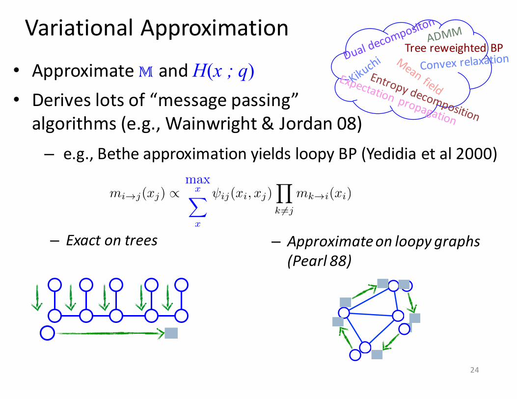
Variational Approximation
• Approximate M and H(x ; q)• Derives lots of “message passing” algorithms (e.g., Wainwright & Jordan 08)
m
i!j
(x
j
) /max
xX
x
ij
(x
i
, x
j
)
Y
k 6=j
m
k!i
(x
i
)
– Exact on trees – Approximate on loopy graphs (Pearl 88)
Tree reweighted BP
– e.g., Bethe approximation yields loopy BP (Yedidia et al 2000)
24
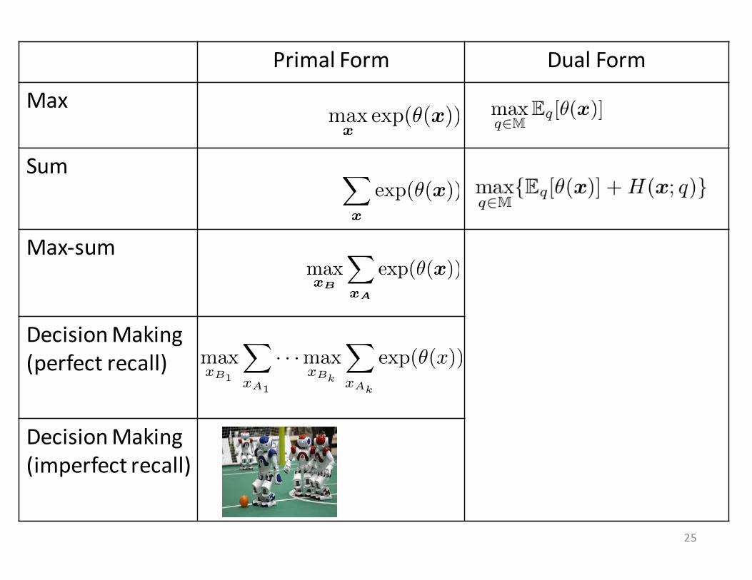
Primal Form Dual Form
Max
Sum
Max-‐sum
Decision Making(perfect recall)
DecisionMaking(imperfect recall)
max
xB1
X
xA1
· · ·max
xBk
X
xAk
exp(✓(x))
max
x
exp(✓(x))
25
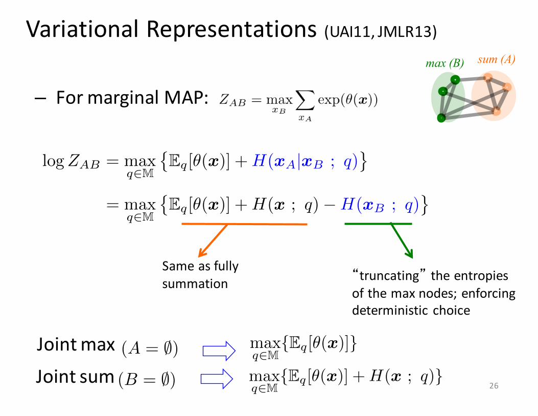
max (B) sum (A)
Variational Representations (UAI11, JMLR13)
– For marginal MAP:
“truncating” the entropies of the max nodes; enforcing deterministic choice
Same as fully summation
logZAB = max
q2M
�Eq[✓(x)] +H(xA|xB ; q)
= max
q2M
�Eq[✓(x)] +H(x ; q)�H(xB ; q)
(B = ;)Joint sumJoint max max
q2M{Eq[✓(x)]}
max
q2M{Eq[✓(x)] +H(x ; q)}
(A = ;)
26
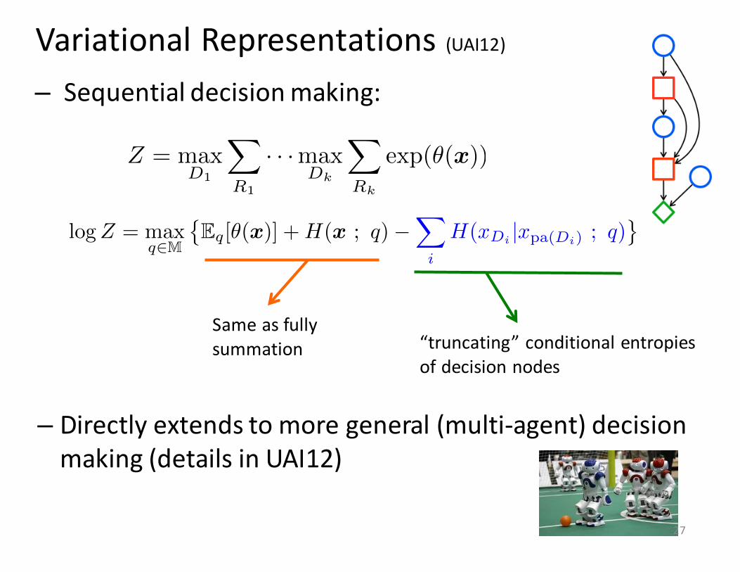
– Sequential decision making:
“truncating” conditional entropies of decision nodes
Z = max
D1
X
R1
· · ·max
Dk
X
Rk
exp(✓(x))
Same as fully summation
Variational Representations (UAI12)
– Directly extends to more general (multi-‐agent) decision making (details in UAI12)
logZ = max
q2M
�Eq[✓(x)] +H(x ; q)�
X
i
H(xDi |xpa(Di) ; q)
27
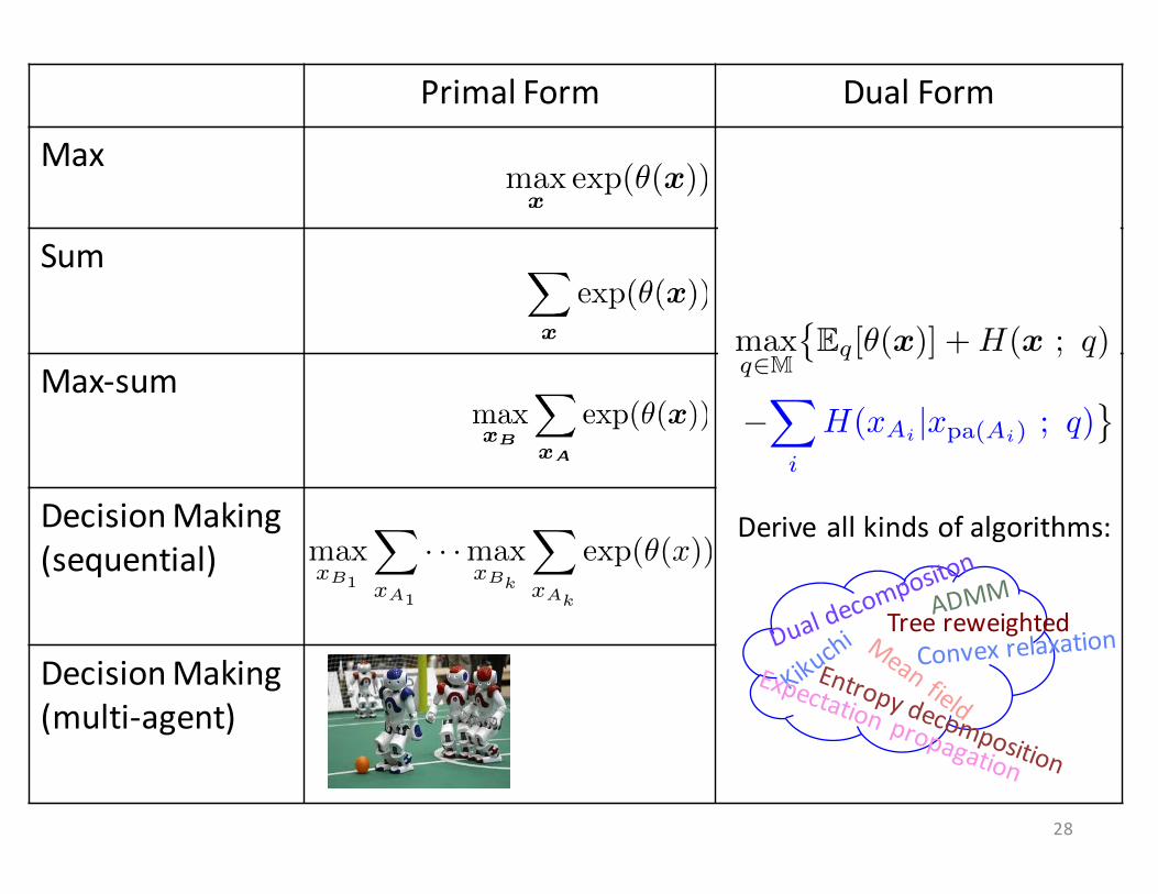
Primal Form Dual Form
Max
Sum
Max-‐sum
Decision Making(sequential)
DecisionMaking(multi-‐agent)
Derive all kinds of algorithms:
Tree reweighted
max
xB1
X
xA1
· · ·max
xBk
X
xAk
exp(✓(x))
max
q2M
�Eq[✓(x)] +H(x ; q)
�X
i
H(xAi |xpa(Ai) ; q)
max
x
exp(✓(x))
28
(Sum-Product)
(Argmax-Product)
max (B) sum (A)
Sum ⇒ Sum∪Max:(Max-Product)
Max ⇒Max:
Max ⇒ Sum:
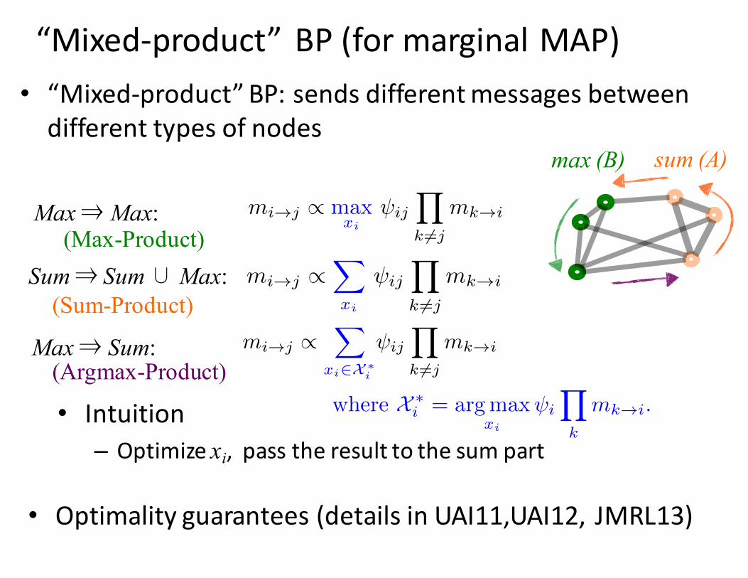
“Mixed-‐product” BP (for marginal MAP)• “Mixed-‐product” BP: sends different messages between different types of nodes
• Optimality guarantees (details in UAI11,UAI12, JMRL13)
TextText
Text
• Intuition– Optimize xi, pass the result to the sum part
mi!j
/ max
xi
ij
Y
k 6=j
mk!i
mi!j
/X
xi
ij
Y
k 6=j
mk!i
mi!j
/X
xi2X⇤i
ij
Y
k 6=j
mk!i
where X ⇤i
= argmax
xi
i
Y
k
mk!i
.
Model Parameter0.5 1 1.5 2 2.5
−0.3
−0.25
−0.2
−0.15
−0.1
−0.05
0
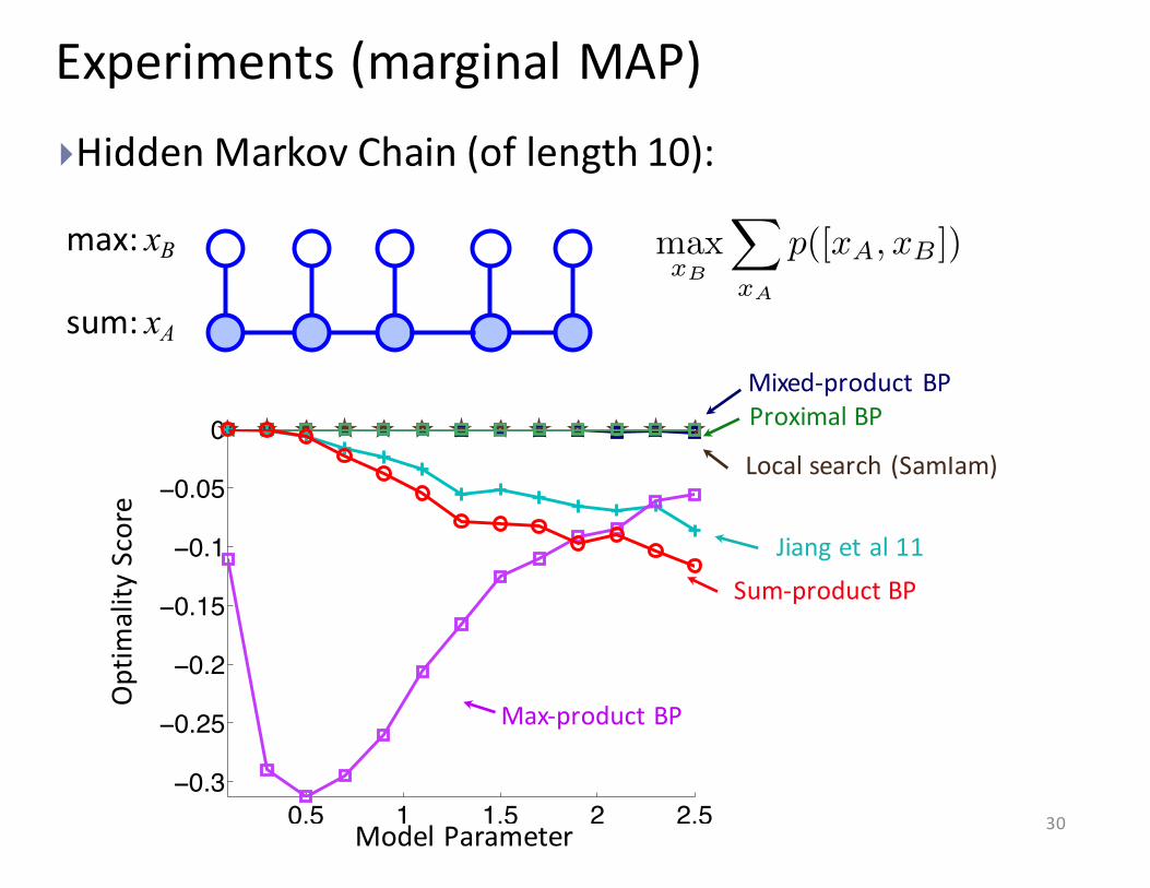
}Hidden Markov Chain (of length 10):
Max-‐product BP
Sum-‐product BPJiang et al 11
Experiments (marginal MAP)
Proximal BP
Local search (SamIam)
Optim
ality
Score
Mixed-‐product BP
max
xB
X
xA
p([x
A
, x
B
])
max: xB
sum: xA
30
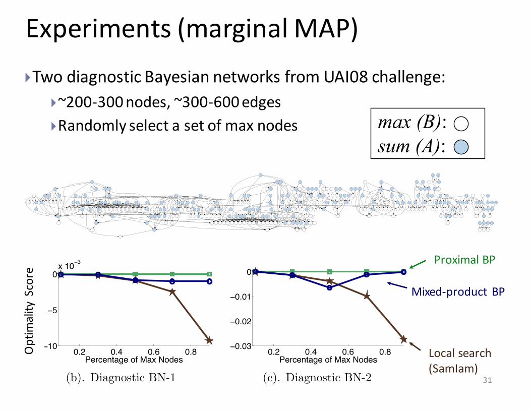
Experiments (marginal MAP)
Variational algorithms for Marginal MAP
(a). The Structure of Diagnostic BN-2, with 50% randomly selected sum nodes shaped.
0.2 0.4 0.6 0.8−10
−5
0x 10−3
Aopr
oxim
ate
Rel
ativ
e Er
ror
Percentage of Max Nodes0.2 0.4 0.6 0.8−0.03
−0.02
−0.01
0
Percentage of Max Nodes
(b). Diagnostic BN-1 (c). Diagnostic BN-2
Proximal (Bethe)Mix−product (Bethe)Local Search (SamIam)
Figure 7: The results on two diagnostic Bayesian networks (BNs) in UAI08 inference chal-lenge. (a) the structure of diagnostic BN-2. (b)-(c) The performances of algorithms onthese two BNs as the percentage of max nodes increases. Averaged on 100 random trials.{fig:uai_result}
Acknowledgments
We thank Arthur Choi for providing help on SamIam. This work was supported in part byNSF grant IIS-1065618 and a Microsoft Research Ph.D Fellowship.
References
F. Altarelli, A. Braunstein, A. Ramezanpour, and R. Zecchina. Stochastic optimization bymessage passing. Journal of Statistical Mechanics: Theory and Experiment, 2011(11):P11009, 2011.
J.R. Birge and F. Louveaux. Introduction to stochastic programming. Springer Verlag, 1997.
S. Boyd, N. Parikh, E. Chu, B. Peleato, and J. Eckstein. Distributed optimization andstatistical learning via the alternating direction method of multipliers. Found. TrendsMach. Learn., 2010.
M.J. Choi, V.Y.F. Tan, A. Anandkumar, and A. Willsky. Learning latent tree graphicalmodels. Journal of Machine Learning Research, 12:1771–1812, 2011.
Thomas M. Cover and Joy A. Thomas. Elements of Information Theory. John Wiley &Sons, INC., 2nd edition, 2006.
C.P. De Campos. New complexity results for MAP in Bayesian networks. In Proceedings ofthe Twenty-Second International Joint Conference on Artificial Intelligence, pages 2100–2106, 2011.
R. Dechter and I. Rish. Mini-buckets: A general scheme for bounded inference. Journal ofthe ACM (JACM), 50(2):107–153, 2003.
29
}Two diagnostic Bayesian networks from UAI08 challenge:}~200-‐300 nodes, ~300-‐600 edges}Randomly select a set of max nodes max (B):
sum (A):
Mixed-‐product BP
Proximal BP
Local search (SamIam)
31
Optimality Score
Structured Prediction with Missing labels
770771772773774775776777778779780781782783784785786787788789790791792793794795796797798799800801802803804805806807808809810811812813814815816817818819820821822823824
825826827828829830831832833834835836837838839840841842843844845846847848849850851852853854855856857858859860861862863864865866867868869870871872873874875876877878879
Marginal Structured SVM with Hidden Variables
0 10 30 50 70 900
5
10
15
20
25
Pecentage of Hidden Variables(%)
Err
or
Ra
te(%
)
LSSVM
HCRFs
MSSVM
(a) (b) (c)
Figure 4. (a) The ground truth image. (b) An example of an observed noisy image. (c) The performance of each algorithmas the percentage of missing labels varies from 10% to 95%. Results are averaged over 5 random trials, each using 10training instances and 10 test instances.
�(yi
, x
i
) = e
yi ⌦ x
i
and pairwise features �(yi
, y
j
) =e
yi ⌦ e
yj 2 R5⇥5 as defined in Nowozin & Lampert(2011), where e
yi is the unit normal vector with entryone on dimension y
i
and ⌦ is the outer product. Theset of missing labels (hidden variables) are determinedat random, in proportions ranging from 10% to 95%.The performance of MSSVM, LSSVM, and HCRFs areevaluated using the CCCP algorithm.
Figure 4 lists the performance of each method as thepercentage of missing labels is increased. We can seethat the performance of LSSVM degrades significantlyas the number of hidden variables grows. Most no-tably, MSSVM is consistently the best method acrossall settings. This can be explained by MSSVM combin-ing both the max-margin property and the improvedrobustness given by properly accounting for uncer-tainty in the hidden labels.
7.3. Object Categorization
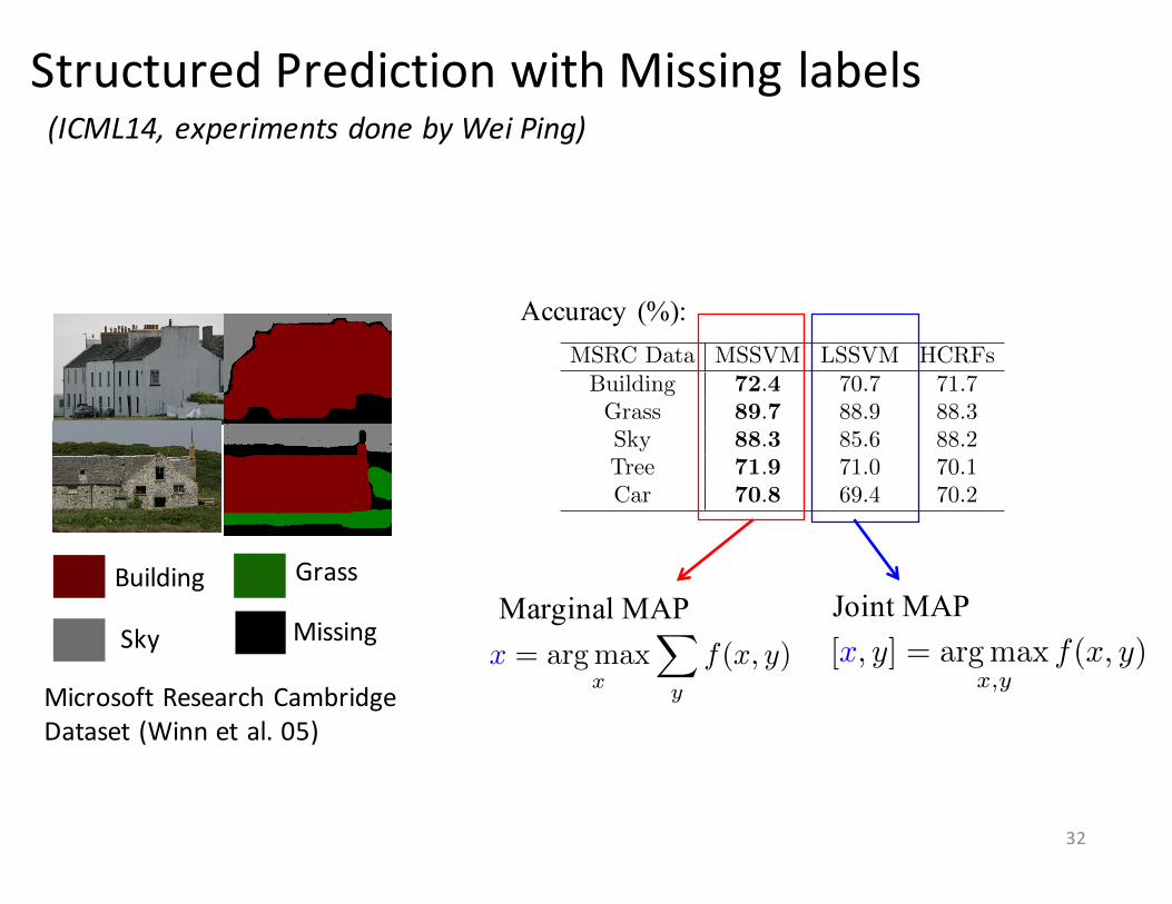
Finally, we evaluate our MSSVM method on the taskof object categorization using partially labeled images.We use the Microsoft Research Cambridge data set(Winn et al., 2005), consisting of 240 images with213⇥320 pixels and their partial pixel-level labelings.Modeled on the approach outlined in Verbeek & Triggs(2007), we use 20⇥20 pixel patches with centers at 10pixel intervals and treat each patch as a node in ourmodel. This results in a 20 ⇥ 31 grid model. Thefeatures of each patch are encoded using texture andcolor descriptors. For texture, we compute the 128-dimensional SIFT descriptor of the patch and vectorquantize it into a 500-word codebook, learned by k-means clustering of all patches in the entire dataset.For color, we take 48-dimensional RGB color his-togram for each patch. In our experiment, we selectthe 5 most frequent categories in the dataset and use2-fold cross validation for testing.
Table 4. Average patch level accuracy (%) of MSSVM,LSSVM, HCRFs for MSRC data by 2-fold cross validation
MSRC Data MSSVM LSSVM HCRFsBuilding 72.4 70.7 71.7Grass 89.7 88.9 88.3Sky 88.3 85.6 88.2Tree 71.9 71.0 70.1Car 70.8 69.4 70.2
Table 4 shows the accuracies of each method acrossthe various categories. Again, we find that MSSVMconsistently outperforms other methods across all cat-egories, which can be explained by both the superiorityof SSVM-based methods and the improved robustnessby accounting for uncertainty in the missing labels.
8. Conclusion
We proposed a novel structured SVM method forstructured prediction with hidden variables. Wedemonstrate that our method consistently outper-forms the state of art in both simulated and real data,especially when the uncertainty of hidden variables islarge. Compared to the popular LSSVM, our MSSVMis easy to optimize due to the smoothness of its ob-jective function. We also provide a unified frameworkwhich includes our method as well as a spectrum ofprevious methods as special cases.
Microsoft Research Cambridge Dataset (Winn et al. 05)
Sky
Building Grass
MissingMarginal MAP Joint MAPx = argmax
x
X
y
f(x, y)
[x, y] = argmax
x,y
f(x, y)
Accuracy (%):
32
(ICML14, experiments done by Wei Ping)
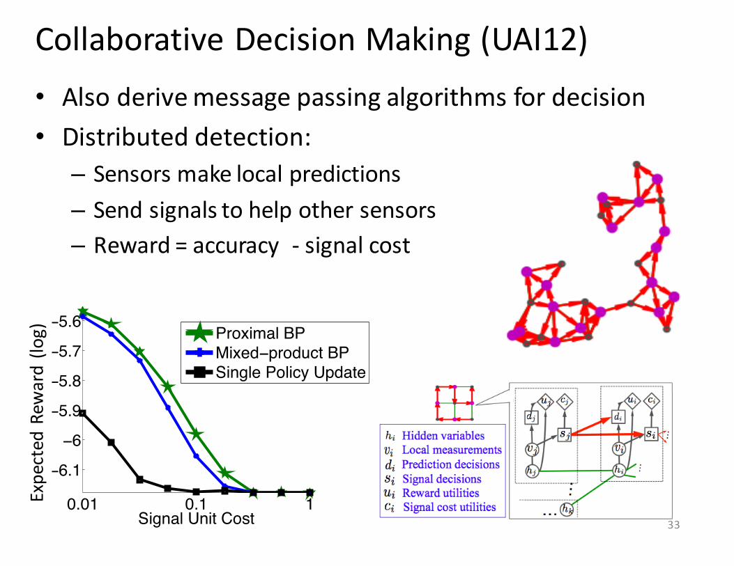
Collaborative Decision Making (UAI12)• Also derive message passing algorithms for decision• Distributed detection:– Sensors make local predictions– Send signals to help other sensors– Reward = accuracy -‐ signal cost
0.01 0.1 1
−6.1
−6
−5.9
−5.8
−5.7
−5.6
log
MEU
Signal Unit Cost
Proximal BPMixed−product BPSingle Policy Update
33
Expected Rew
ard (lo
g)
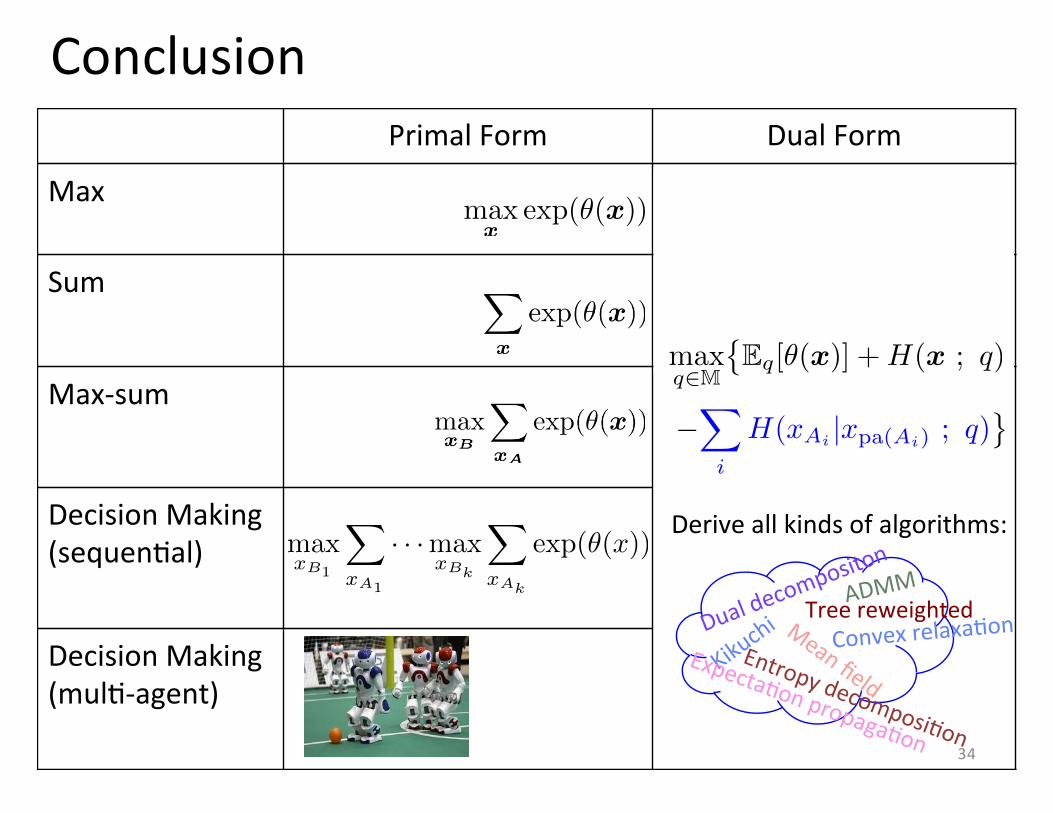
Conclusion
34
Primal'Form' Dual'Form'
Max''
Sum'
Max/sum'
Decision'Making'(sequen8al)'
Decision'Making'(mul8/agent)'
Derive'all'kinds'of'algorithms:''
Mean'field'Kikuch
i'' Tree'reweighted'Dual'deco
mpositon
'
ADMM'
Entropy'decomposi8on'
Expecta8on'propaga8on'
Convex'relaxa8on'
max
xB1
X
xA1
· · ·max
xBk
X
xAk
exp(✓(x))
max
q2M
�Eq[✓(x)] +H(x ; q)
�X
i
H(xAi |xpa(Ai) ; q)
max
x
exp(✓(x))

Thank you!
35