Introduction to Probabilistic Graphical Modelspub.ist.ac.at/~chl/courses/PGM_W16/part9.pdf · Introduction to Probabilistic Graphical Models Christoph Lampert ... (Integer) Linear

Energy Minimization (Integer) Linear Programming Local Search Sampling Sampling Loss functions

Introduction to Probabilistic Graphical Models

Christoph Lampert

IST Austria (Institute of Science and Technology Austria)

1 / 40


Schedule

Refresher of ProbabilitiesIntroduction to Probabilistic Graphical Models

Probabilistic InferenceLearning Conditional Random Fields

MAP Prediction / Energy MinimizationLearning Structured Support Vector Machines

Links to slide download: http://pub.ist.ac.at/~chl/courses/PGM_W16/

Password for ZIP files (if any): pgm2016

Email for questions, suggestions or typos that you found: [email protected]

2 / 40

http://pub.ist.ac.at/~chl/courses/PGM_W16/

[email protected]


Supervised Learning Problem

I Given training examples (x1, y1), . . . , (xN , yN) ∈ X × Yx ∈ X : input, e.g. imagey ∈ Y: structured output, e.g. human pose, sentence

Images: HumanEva dataset

Goal: be able to make predictions for new inputs, i.e. learn a function f : X → Y.3 / 40


Supervised Learning Problem

Step 1: define a proper graph structure of X and Y

. . .

Ytop

Yhead

YtorsoYrarm

Yrhnd

Yrleg

Yrfoot Ylfoot

Ylleg

Ylarm

Ylhnd

X

. . .

. . .

. . .

. . .

. . .

. . .

. . .

. . .

. . .

. . .

F(1)

top

F(2)

top,head

Step 2: define a proper parameterization of p(y |x ; θ) p(y |x ; θ) =1

Ze∑d

i=1 θiφi (x ,y)

Step 3: learn parameters θ∗ from training data e.g. maximum likelihood

Step 4: for new x ∈ X , make predictione.g. y∗ = argmax

y∈Yp(y |x ; θ∗)

(→ today)

4 / 40

MAP Prediction / Energy Minimization

argmaxy p(y |x) / argminy E (y , x)


MAP Prediction / Energy Minimization

I Exact Energy Minimization

I Belief Propagation on chains/trees

I Graph-Cuts for submodular energies

I Integer Linear Programming

I Approximate Energy Minimization

I Linear Programming Relaxations

I Local Search Methods

I Iterative Conditional Modes

I Multi-label Graph Cuts

I Simulated Annealing

6 / 40


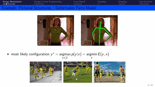
Example: Pictorial Structures / Deformable Parts Model

. . .

Ytop

Yhead

YtorsoYrarm

Yrhnd

Yrleg

Yrfoot Ylfoot

Ylleg

Ylarm

Ylhnd

X

. . .

. . .

. . .

. . .

. . .

. . .

. . .

. . .

. . .

. . .

F(1)

top

F(2)

top,head

I Tree-structured model for articulated pose(Felzenszwalb and Huttenlocher, 2000), (Fischler and Elschlager, 1973),

(Yang and Ramanan, 2013), (Pishchulin et al., 2012)

7 / 40


Example: Pictorial Structures / Deformable Parts Model

I most likely configuration y∗ = argmaxy∈Y

p(y |x) = argminy

E (y , x)

8 / 40


Energy Minimization – Belief Propagation

Chain model: same trick as for inference: belief propagation

miny

E (y) = minyi ,yj ,yk ,yl

EF (yi , yj) + EG (yj , yk) + EH(yk , yl)

= minyi ,yj

[EF (yi , yj) + min

yk

[EG (yj , yk) + min

ylEH(yk , yl)︸︷︷︸

rH→Yk(yk )

]]

= minyi ,yj

[EF (yi , yj) + min

ykEG (yj , yk) + rH→Yk

(yk)︸︷︷︸rG→Yj

(yj )

]

= minyi ,yj

[EF (yi , yj) + rG→Yj

(yj)]

. . .

I actual argmax by backtracking which choices were maximal

9 / 40




miny



= minyi ,yj

[EF (yi , yj) + min

yk

[EG (yj , yk) + min

ylEH(yk , yl)

]]

= minyi ,yj

[EF (yi , yj) + min

yk

[EG (yj , yk) + min


rH→Yk(yk )

]]

= minyi ,yj

[EF (yi , yj) + min



(yj )

]

= minyi ,yj


(yj)]

. . .


9 / 40




miny



= minyi ,yj

[EF (yi , yj) + min

yk

[EG (yj , yk) + min


rH→Yk(yk )

]]

= minyi ,yj

[EF (yi , yj) + min



(yj )

]

= minyi ,yj


(yj)]

. . .


9 / 40




Yi Yj Yk Yl

F G H

rH→Yk∈ RYk

miny



= minyi ,yj

[EF (yi , yj) + min

yk

[EG (yj , yk) + min


rH→Yk(yk )

]]

= minyi ,yj

[EF (yi , yj) + min


(yk)]

= minyi ,yj

[EF (yi , yj) + min



(yj )

]

= minyi ,yj


(yj)]

. . .


9 / 40




Yi Yj Yk Yl

F G H

rH→Yk∈ RYk

miny



= minyi ,yj

[EF (yi , yj) + min

yk

[EG (yj , yk) + min


rH→Yk(yk )

]]

= minyi ,yj

[EF (yi , yj) + min



(yj )

]

= minyi ,yj


(yj)]

. . .


9 / 40




Yi Yj Yk

F G HYl

rG→Yj∈ RYj

miny



= minyi ,yj

[EF (yi , yj) + min

yk

[EG (yj , yk) + min


rH→Yk(yk )

]]

= minyi ,yj

[EF (yi , yj) + min



(yj )

]

= minyi ,yj


(yj)]

. . .


9 / 40




miny



= minyi ,yj

[EF (yi , yj) + min

yk

[EG (yj , yk) + min


rH→Yk(yk )

]]

= minyi ,yj

[EF (yi , yj) + min



(yj )

]

= minyi ,yj


(yj)]

. . .


9 / 40



Tree models:

Yi Yj Yk

F G H

I

Ym

rH→Yk(yk)

rI→Yk(yk)

Yl

qYk→G(yk)

I qH→Yk(yk) = minyl EH(yk , yl)

I qI→Yk(yk) = minym EI (yk , ym)

I qYk→G (yk) = qH→Yk(yk) + qI→Yk

(yk)

min-sum (more commonly max-sum) belief propagation

10 / 40


Belief Propagation in Cyclic Graphs

Yi Yj Yk

Yl Ym Yn

Yo Yp Yq

A B

F G

K L

C D E

H I J

Yi Yj Yk

Yl Ym Yn

Yo Yp Yq

A B

F G

K L

C D E

H I J

Loopy Max-Sum Belief Propagation

Same problem as in probabilistic inference:

I no guarantee of convergence

I no guarantee of optimality

Some convergent variants exist, e.g. TRW-S [Kolmogorov, PAMI 2006]

11 / 40


Cyclic Graphs

In general, MAP prediction/energy minimization in models with cycles or higher-order terms isintractable (NP-hard).

Some important exceptions:

I low tree-width [Lauritzen, Spiegelhalter, 1988]

I binary states, pairwise submodular interactions[Boykov, Jolly, 2001]

I binary states, only pairwise interactions, planargraph [Globerson, Jaakkola, 2006]

I special (Potts Pn) higher order factors [Kohli, Kumar,

2007]

I perfect graph structure [Jebara, 2009]

Yi Yj

Yk Yl

12 / 40


Submodular Energy Functions

I Binary variables: Yi = {0, 1} for all i ∈ VI Energy function: unary and pairwise factors

E (y ; x ,w) =∑i∈V

Ei (yi ) +∑

(i ,j)∈EEij(yi , yj)

Yi Yj

Xi Xj

I Restriction 1 (without loss of generality):

Ei (yi ) ≥ 0

(always achievable by adding a constant to E )

I Restriction 2 (submodularity):

Eij(yi , yj) = 0, if yi = yj ,

Eij(yi , yj) = Eij(yj , yi ) ≥ 0, otherwise.

”neighbors prefer to have the same labels”

13 / 40


Submodular Energy Functions

I Binary variables: Yi = {0, 1} for all i ∈ VI Energy function: unary and pairwise factors

E (y ; x ,w) =∑i∈V

Ei (yi ) +∑

(i ,j)∈EEij(yi , yj)

Yi Yj

Xi Xj

I Restriction 1 (without loss of generality):

Ei (yi ) ≥ 0

(always achievable by adding a constant to E )

I Restriction 2 (submodularity):

Eij(yi , yj) = 0, if yi = yj ,

Eij(yi , yj) = Eij(yj , yi ) ≥ 0, otherwise.

”neighbors prefer to have the same labels”13 / 40


Graph-Cuts Algorithm for Submodular Energy Minimization [Greig et al., 1989]

If conditions are fulfilled, energy minimization can be performed by a solving s-t-mincut:

I construct auxiliary undirected graph

I one node {i}i∈V per variable

I two extra nodes: source s, sink t

I weighted edges

Edge weight

{i , j} Eij(yi = 0, yj = 1){i , s} Ei (yi = 1){i , t} Ei (yi = 0)

I find s-t-cut of minimal weight(polynomial time using max-flow theorem)

i j k

l m n

s

t

{i, s}

{i, t}

From minimal weight cut we recover labeling of minimal energy:I y∗i = 1 if edge {i , s} is cut. Otherwise y∗i = 0

14 / 40


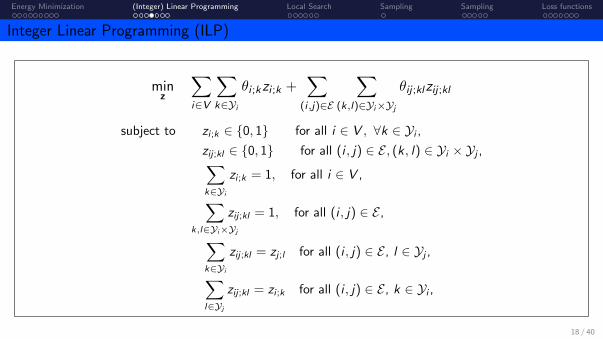
Integer Linear Programming (ILP)

General energy E (y) =∑

F EF (yF )

I variables with more than 2 states

I higher-order factors (more than 2 variables)

I non-submodular factors

Yi Yj

Yk Yl

Formulate as integer linear program (ILP)

I linear objective function

I linear constraints

I variables to optimize over are integer-valued

ILPs are in general NP-hard, but some individual instances can be solved

I standard optimization toolboxes: e.g. CPLEX, Gurobi, COIN-OR, . . .

15 / 40



Example:

Encode assignment in indicator variables:I z1 ∈ {0, 1}Y1 z1;k = 1 ⇔ Jy1 = kKI z2 ∈ {0, 1}Y2 z2;l = 1 ⇔ Jy2 = lKI z12 ∈ {0, 1}Y1×Y2 z12;kl = 1 ⇔ Jy1 = k ∧ y2 = lK

Consistency Constraints:∑k∈Y1

z1;k = 1,∑l∈Y2

z2;l = 1,∑

k,l∈Y1×Y2

z12;kl = 1 (indicator property)

∑k∈Y1

z12;kl = z2;l

∑l∈Y2

z12;kl = z1;k (consistency)

16 / 40



Example: Y1 Y2

Y1 Y1 × Y2 Y2

y1 = 2

y2 = 3

(y1, y2) = (2, 3)

Encode assignment in indicator variables:I z1 ∈ {0, 1}Y1 , z2 ∈ {0, 1}Y2 , z12 ∈ {0, 1}Y1×Y2

Consistency Constraints:∑k∈Y1

z1;k = 1,∑l∈Y2

z2;l = 1,∑

k,l∈Y1×Y2

z12;kl = 1 (indicator property)

∑k∈Y1

z12;kl = z2;l

∑l∈Y2

z12;kl = z1;k (consistency)

16 / 40



Example: E (y1, y2) = E1(y1) + E12(y1, y2) + E2(y2)Y1 Y2

Y1 Y1 × Y2 Y2

θ1 θ1,2 θ2

Define coefficient vectors:I θ1 ∈ RY1 θ1;k = E1(k)

I θ2 ∈ RY2 θ2;l = E2(l)

I θ12 ∈ RY1×Y2 θ12;kl = E1,2(k, l)

Energy is a linear function of unknown z:

E (y1, y2) =∑i∈V

∑k∈Yi

θi ;kJyi = kK +∑i ,j∈E

∑k,l∈Yi×Yj

θij ;klJyi = k ∧ yj = lK

17 / 40



Example: E (y1, y2) = E1(y1) + E12(y1, y2) + E2(y2)Y1 Y2

Y1 Y1 × Y2 Y2

θ1 θ1,2 θ2

Define coefficient vectors:I θ1 ∈ RY1 θ1;k = E1(k)

I θ2 ∈ RY2 θ2;l = E2(l)

I θ12 ∈ RY1×Y2 θ12;kl = E1,2(k, l)

Energy is a linear function of unknown z:

E (y1, y2) =∑i∈V

∑k∈Yi

θi ;kzi ;k +∑

(i ,j)∈E

∑(k,l)∈Yi×Yj

θij ;klzij ;kl

17 / 40



minz

∑i∈V

∑k∈Yi

θi ;kzi ;k +∑

(i ,j)∈E

∑(k,l)∈Yi×Yj

θij ;klzij ;kl

subject to zi ;k ∈ {0, 1} for all i ∈ V , ∀k ∈ Yi ,zij ;kl ∈ {0, 1} for all (i , j) ∈ E , (k, l) ∈ Yi × Yj ,∑k∈Yi

zi ;k = 1, for all i ∈ V ,

∑k,l∈Yi×Yj

zij ;kl = 1, for all (i , j) ∈ E ,

∑k∈Yi

zij ;kl = zj ;l for all (i , j) ∈ E , l ∈ Yj ,∑l∈Yj

zij ;kl = zi ;k for all (i , j) ∈ E , k ∈ Yi ,

NP-hard to solve because of integrality constraints.

18 / 40



minz

∑i∈V

∑k∈Yi

θi ;kzi ;k +∑

(i ,j)∈E

∑(k,l)∈Yi×Yj

θij ;klzij ;kl

subject to zi ;k ∈ {0, 1} for all i ∈ V , ∀k ∈ Yi ,zij ;kl ∈ {0, 1} for all (i , j) ∈ E , (k, l) ∈ Yi × Yj ,∑k∈Yi


∑k,l∈Yi×Yj


∑k∈Yi



NP-hard to solve because of integrality constraints. 18 / 40


Linear Programming (LP) Relaxation

minz

∑i∈V

∑k∈Yi

θi ;kzi ;k +∑

(i ,j)∈E

∑(k,l)∈Yi×Yj

θij ;klzij ;kl

subject to ((((((hhhhhhzi ;k ∈ {0, 1} zi ;k ∈ [0, 1] for all i ∈ V , ∀k ∈ Yi ,((((((hhhhhhzij ;kl ∈ {0, 1} zij ;kl ∈ [0, 1] for all (i , j) ∈ E , (k, l) ∈ Yi × Yj ,∑k∈Yi


∑k,l∈Yi×Yj


∑k∈Yi



Relax constraints → optimization problem becomes tractable 19 / 40



Solution z∗LP might have fractional values

I → no corresponding labeling y ∈ YI → round LP solution to {0, 1} values

Problem:I rounded solution usually not optimal, i.e. not identical to ILP solution

LP relaxations perform approximate energy minimization20 / 40



Example: color quantization

Example: stereo reconstruction

Images: Berkeley Segmentation Dataset

21 / 40


Local Search

Avoid getting fractional solutions: energy minimization by local search

I choose starting labeling y0

I construct neighborhood N (y0) ⊂ Y of labelings

I find minimizer within neighborhood, y1 = argminy∈N (y0) E (y)

I iterate until no more changes

22 / 40


Local Search


y0

Y


I construct neighborhood N (y0) ⊂ Y of labelingsI find minimizer within neighborhood, y1 = argminy∈N (y0) E (y)I iterate until no more changes

22 / 40


Local Search


y0

N (y0)

Y


I construct neighborhood N (y0) ⊂ Y of labelings

I find minimizer within neighborhood, y1 = argminy∈N (y0) E (y)I iterate until no more changes

22 / 40


Local Search


y0 y1

N (y0)

Y


I construct neighborhood N (y0) ⊂ Y of labelingsI find minimizer within neighborhood, y1 = argminy∈N (y0) E (y)

I iterate until no more changes

22 / 40


Local Search


y0 y1

N (y0) N (y1)

y2

N (y2)

y3

y∗

N (y3)

N (y∗)

Y


I construct neighborhood N (y0) ⊂ Y of labelingsI find minimizer within neighborhood, y1 = argminy∈N (y0) E (y)I iterate until no more changes

22 / 40


Iterated Conditional Modes (ICM) [Besag, 1986]

Define local neighborhoods:I Ni (y) = {(y1, . . . , yi−1, y , yi+1, . . . , yn)|y ∈ Yi} for i ∈ V .

all labeling reachable from y by changing value of yi

. . .

ICM procedure:I neighborhood N (y) =

⋃i∈V Ni (y)

all states reachable from y by changing a single variable

I y t+1 = argminy∈N (y t)

E (y) by exhaustive search (∑

i |Yi | evaluations)

23 / 40






⋃i∈V Ni (y)





Observation: larger neighborhood sizes are betterI ICM: |N (y)| linear in |V |→ many iterations to explore exponentially large Y

I ideal: |N (y)| exponential in |V |,→ but: we must ensure that argminy∈N (y) E (y) remains tractable

23 / 40






⋃i∈V Ni (y)





Observation: larger neighborhood sizes are betterI ICM: |N (y)| linear in |V |→ many iterations to explore exponentially large Y

I ideal: |N (y)| exponential in |V |,→ but: we must ensure that argminy∈N (y) E (y) remains tractable

23 / 40


Multilabel Graph-Cut: α-expansion

I E (y) with unary and pairwise termsI Yi = L = {1, . . . ,K} for i ∈ V (multi-class)

Example: semantic segmentation

24 / 40




Example: semantic segmentation

24 / 40




Algorithm

I initialize y0 arbitrarily (e.g. everything label 0)I repeat

I for any α ∈ LI construct neighborhood:

N (y) ={

(y1, . . . , y|V |) : yi ∈ {yi , α}}

”each variable can keep its value or switch to α”I solve y ← argminy∈N (y) E (y)

I until y has not changed for a whole iteration

24 / 40



Theorem [Boykov et al. 2001]

If all pairwise terms are metric, i.e. for all (i , j) ∈ E

Eij(k, l) ≥ 0 with Eij(k , l) = 0⇔ k = l

Eij(k, l) = Eij(l , k)

Eij(k, l) ≤ Eij(k,m) + Eij(m, l) for all k , l ,m

Then argminy∈N (y) E (y) can be solved optimally using GraphCut.

Theorem [Veksler 2001]. The solution, yα, returned by α-expansion fulfills

E (yα) ≤ 2c ·miny∈Y

E (y) for c = max(i ,j)∈E

maxk 6=l Eij(k , l)

mink 6=l Eij(k , l)

25 / 40


Example: Semantic Segmentation

E (y) =∑i∈V

Ei (yi ) + λ∑

(i ,j)∈EJyi 6= yjK ”Potts model”

I Eij(k, l) ≥ 0 Eij(k, l) = 0 ⇔ k = l Eij(k , l) = Eij(l , k) X

I Eij(k , l) ≤ Eij(k,m) + Eij(m, l) X

I c = max(i ,j)∈Emaxk 6=l Eij (k,l)mink 6=l Eij (k,l)

= 1

I factor-2 approximation guarantee: E (yα) ≤ 2 miny∈Y E (y)

26 / 40


Example: Stereo Estimation

E (y) =∑i∈V

Ei (yi ) + λ∑

(i ,j)∈E|yi − yj |

I |yi − yj | is metric X

I c = max(i ,j)∈Emaxk 6=l Eij (k,l)mink 6=l Eij (k,l)

= |L − 1|I weak guarantees, but often close to optimal labelings in practice

Images: Middlebury stereo vision dataset

27 / 40


Sampling

Sampling was a general purpose probabilistic inference method. Can we use it for prediction?

MAP prediction from samples:

I S = {x1, . . . , xN} samples from p(x)

I x∗ ← argmaxx∈S p(x)

I output x∗

Problem:

I will need many samples

I with x∗ = argmaxx∈X p(x): Pr(x∗ 6= x∗) = (1− p(x∗))N ≈ 1− Np(x∗)I for graphical model, probability values are tiny, e.g. p(x∗) = 10−100 can easily happen

I N ≈ 5 · 1099 required to have 50% chance28 / 40


Sampling

Let’s construct a better distribution:

Idea 2: Form a new distribution, p′, that has all its probability mass at the location ofmaximum of p

p′(x) = Jx = x∗K for x∗ = argmaxx∈X

p(x)

and sample from it

Advantage: we need only 1 sample

Problem: to define p′ we need x∗, which is what we’re after.

29 / 40


Sampling

Idea 3: do the same as idea 2, but more implicitly:

pβ(x) ∝ [p(x)]β for very large β

4 2 0 2 40.0

0.2

0.4

0.6

0.8

1.0

1.2

p(x)

4 2 0 2 40.0

0.2

0.4

0.6

0.8

1.0

1.2

[p(x)]2

4 2 0 2 40.0

0.2

0.4

0.6

0.8

1.0

1.2

[p(x)]10

4 2 0 2 40.0

0.2

0.4

0.6

0.8

1.0

1.2

[p(x)]100

Particularly easy for distributions in exponential form: p(x)∝e−E(x) becomes pβ(x)∝e−βE(x)

30 / 40


Simulated Annealing

Practical questions: How to choose β? How to sample from pβ?

These are often coupled, especially sampling works by a Monte Carlo Markov Chain (MCMC):I samples x1, x2, . . . from MCMC are dependent,I two consecutive samples are often similar to each other → random walk,I for a distribution with multiple peaks that are separated by a low-probability region,

MCMC sampling will jump around a peak, but very rarely switch peaks

4 2 0 2 40.0

0.2

0.4

0.6

0.8

1.0

1.2

p(x)

4 2 0 2 40.0

0.2

0.4

0.6

0.8

1.0

1.2

[p(x)]2

4 2 0 2 40.0

0.2

0.4

0.6

0.8

1.0

1.2

[p(x)]10

4 2 0 2 40.0

0.2

0.4

0.6

0.8

1.0

1.2

[p(x)]100

31 / 40


Sampling

Image: By Kingpin13 - Own work, CC0, https://commons.wikimedia.org/w/index.php?curid=2501076332 / 40


MAP Prediction / Energy Minimization – Summary

Task: compute argminy∈Y E (y |x)

Exact Energy Minimization

Only possible for certain models:

I trees/forests: max-sum belief propagation

I general graphs: junction chain algorithm (if tractable)

I submodular energies: GraphCut

I general graphs: integer linear programming (if tractable)

Approximate Energy Minimization

Many techniques with different properties and guarantees:

I linear programs relaxations, ICM, α-expansion

Best choices depends on model and requirements.33 / 40


Loss functions

34 / 40


Loss functions

We model structured data, e.g. y = (y1, . . . , ym). What makes a good prediction?

I The loss function is application dependent

∆ : Y × Y → R+,

35 / 40


Example 1: 0/1 loss

Loss is 0 for perfect prediction, 1 otherwise:

∆0/1(y , y) = Jy 6= yK =

{0 if y = y1 otherwise

Every mistake is equally bad. Rarely very useful for structured data, e.g.

I handwriting recognition: one letter wrong is as bad as all letters wrong

I image segmentation: one pixel wrong is as bad as all pixels wrong

I automatic translation: a missing article is as bad as completely random output

36 / 40


Example 2: Hamming loss

Count the number of mislabeled variables:

∆H(y , y) =1

m

m∑i=1

Jym 6= ymK

x : I need a coffee break

y : subject verb article object object

y : subject verb article object verb

Jym 6= ymK 0 0 0 0 1

→ ∆H(y , y) = 0.2

Often used for graph labeling tasks, e.g. image segmentation, natural language processing, . . .

37 / 40


Example 3: Squared error

If the individual variables yi are numeric, e.g. pixel intensities,object locations, etc.

Sum of squared errors

∆Q(y , y) =1

m

m∑i=1

‖yi − yi‖2.

Used, e.g., in stereo reconstruction, optical flow estimation, . . .

38 / 40


Example 4: Task specific losses

Object detection

I bounding boxes, or

I arbitrarily shaped regionsground truth

detection

image

Intersection-over-union loss:

∆IoU(y , y) = 1− area(y ∩ y)

area(y ∪ y)= 1 −

Used, e.g., in PASCAL VOC challenges for object detection, because its scale-invariance.

39 / 40


Making Optimal Predictions

Given a structured distribution p(x , y) or p(y |x), what’s the best y to predict?

Decision theory: pick y∗ that causes minimal expected loss:

y∗ = argminy∈Y

Ey∼p(y |x){∆(y , y)} = argminy∈Y

∑y∈Y

∆(y , y)p(y |x)

For many loss functions not tractable to compute, but some exceptions:

I R∆0/1(y) = 1− p(y), so y∗ = argmaxy p(y) → use MAP prediction

I R∆H(y) = 1−∑i∈V p(yi ), so y∗ = (y∗1 , . . . , y

∗n ) with y∗i = argmax

k∈Yip(yi = k)

→ use marginal inference

40 / 40

Documents

Introduction to Probabilistic Graphical Modelspub.ist.ac.at/~chl/courses/PGM_W16/part9.pdf · Introduction to Probabilistic Graphical Models Christoph Lampert ... (Integer) Linear