Thermodynamics and complexity of simple transport phenomena

Owen G. Jepps∗

Lagrange Fellow, Dipartimento di Matematica, Politecnico di Torino,

Corso Duca degli Abruzzi 24, 10129 Torino, Italy

Lamberto Rondoni†

Dipartimento di Matematica and INFM, Politecnico di Torino,

Corso Duca degli Abruzzi 24, 10129 Torino, Italy

(Dated: November 19, 2005)

We examine the transport behaviour of non-interacting particles in a simple chan-

nel billiard, at equilibrium and in the presence of an external field. We observe a

range of sub-diffusive, diffusive, and super-diffusive transport behaviours. We find

nonequilibrium transport that is inconsistent with the equilibrium behaviour, indi-

cating that a linear regime does not exist for this system. However, it may be possible

to construct a “weak” linear regime that leads to consistency between the equilib-

rium and nonequilibrium results. Despite the non-chaotic nature of the dynamics,

we observe greater unpredictability in the transport properties than is observed for

chaotic systems. This observation seems at odds with existing complexity measures,

motivating some new definitions of complexity that are relevant for transport phe-

nomena.

PACS numbers: 05.20.-y, 05.60.-k, 05.90.+m, 89.75.-k

I. INTRODUCTION

One of the fundamental aims of statistical mechanics is to shed light upon the relationship

between the macroscopic properties of a system and its underlying microscopic behaviour.

In the development of such a relationship, conditions of “molecular chaos” on the nature of

∗Electronic address: jepps@calvino.polito.it†Electronic address: lamberto.rondoni@polito.it

2

the microscopic dynamics play a crucial role. The nature of such conditions is a subject of

ongoing research in theories of nonequilibrium systems.

For equilibrium systems, the assumption that a system is ergodic — the Ergodic Hypoth-

esis (EH) — allows one to associate the system’s macroscopic, thermodynamic properties

with its microscopic, mechanical properties. However, ergodicity is notoriously difficult to

prove, and is known to be violated in many cases of physical interest. Despite this, ergod-

icity is still assumed for the purpose of extracting macrosopic information from microscopic

models, largely on the basis that thermodynamic data thus generated appear consistent

with observations of real physical systems. At present there is a wide body of results on

the applicability of the EH, and theoretical explanations of why it should work have been

available for quite some time [1, 2].

In the literature of nonequilibrium systems, conditions of molecular chaos are present

in the form of various “Chaotic Hypotheses” (CH), which have been made either explicitly

or implicitly (see, e.g., Refs.[3, 4]). In constrast with the EH, the CH are not completely

understood yet, and the question of how much “molecular chaos” is sufficient to explain the

observed macroscopic behaviour remains elusive [5]. For instance, recent results indicate

that thermodynamic-like connections between the microscopic and macroscopic nature of

a particle system can be forged for weaker-than-chaotic dynamical systems. In particular,

behaviours reminiscent of normal diffusion and heat conduction have been observed in polyg-

onal billiards [6, 7], where the dynamics is not chaotic. There are various numerical and

mathematical works on the ergodic, mixing and transport properties of irrational polygons,

see, for instance, Refs.[6–13]. However, the models are limited in number, the triangular

billiards being the most studied models, and many questions concerning them remain open.

Despite the vanishing topological entropy of polygonal channels, pairs of orbits almost al-

ways separate [14]. Consequently, these systems exhibit a certain sensitive dependence on

the initial conditions, and their dynamics may appear highly disordered, indistinguishable

to the eye from chaotic motions. However, such non-chaotic dynamics would represent an

extremely weak condition on the required molecular chaos.

Diffusive behaviour has also been observed in non-chaotic one dimensional lattices of

maps, and in the Ehrenfest wind-tree model [43], with spatial quenched disorder [15, 16].

Furthermore, the Gallivotti-Cohen Fluctuation Theorem, which invokes a “Chaotic Hypoth-

esis” [3], has been verified over an initial diffusive phase of transport in a nonequilibrium

3

version of the periodic Ehrenfest wind-tree model [17], and in a model of a mechanical

“pump”, with flat sides [18].

If these results are indicative of thermodynamic connections between microscopic and

macroscopic behaviour, in systems that do not exhibit chaotic behaviour, then they implicitly

call into question the nature of current Chaotic Hypotheses. It is, therefore, of interest

to explore such non-defocussing systems in greater detail, in order to understand more

deeply the nature of such apparently thermodynamic behaviour. In addition to these more

fundamental issues, there is also the practical consideration of the study of transport in

porous media. In certain applications of porous media, such as gas separation and storage,

or the controlled delivery of pharmaceuticals, the accommodation coefficient (indicating the

degree of momentum exchange between fluid molecules and the pore wall) can be exceedingly

low. Consequently, over finite times (and finite pore lengths), the transport behaviour in such

a pore should be well approximated by the behaviour in polygonal channels. Furthermore,

in systems where the molecular size is of the same order as the pore width, the transport

behaviour is dominated by solid-fluid interactions at laboratory temperatures and pressures

[19]. In this respect, the systems studied in this paper resemble transport in microporous

membranes at low (but practically relevant) densities, where interactions are rare.

In this paper, we consider the equilibrium and nonequilibrium mass transport of point

particles in a simple two-dimensional polygonal channel, described in section II. We examine

the average transport behaviour of particles in the channel, in particular the diffusive be-

haviour, as outlined in section III. Despite being arguably the simplest particle system that

could be conceived, we observe (in section IV) a surprising array of transport behaviours.

While certain properties of the system demonstrate almost trivial behaviour, other properties

display an unpredictable richness, which can be expressed through a sensitive dependence

of the macroscopic behaviour on the parameters which define the boundary geometry. We

observe transport behaviour, which can be sub-diffusive, super-diffusive, or apparently dif-

fusive (without excluding the possibility of a ln t tail [20]), and which depends strongly on

the boundary geometry. We find that apparently diffusive behaviour is straightfoward to

obtain, despite the absense of chaos (in the sense of positive Lyapunov exponenets), and

the absense of quenched disorder. However, for those systems that are apparently diffusive

at equilibrium, we fail to observe a linear regime in the nonequilibrium behaviour. These

results suggest a lack of fundamentally thermodynamic behaviour, both in the dependence

4

on the geometry of the transport law, and of the lack of a linear response. Whilst the

system may display ostensibly thermodynamic behaviour, this thermodynamic relationship

does not bear closer scrutiny.

In our view, the dependence of the mass transport on the geometry of the system char-

acterizes such transport as “complex”. Notions of complexity of billiards dynamics, based

on symbolic dynamics, are commonly considered [21, 22]. Using these measures, chaotic

systems would be considered much more complex than non-chaotic systems — whereas the

“symbolic richness” of a chaotic system grows exponentially in time, non-chaotic systems

exhibit sub-exponential growth [21]. These measures represent unpredictability at a mi-

croscopic viewpoint. However, from the macroscopic perspective, the non-chaotic systems

show a much greater diversity, and hence unpredictablility, in their behaviour as a function

of system parameters. While the variation of transport properties with system parameters

is known to be irregular in certain chaotic systems [23–27], the mass transport law in chaotic

systems is usually diffusive in nature (importantly, the irregular behaviour does not neces-

sarily prevent a linear regime, close to equilibrium [28–30]). For the non-chaotic systems

we examine, we observe an additional degree of unpredictability regarding the nature of the

transport law itself. This result would seem to indicate that non-chaotic systems should be

more complex than chaotic systems, a conclusion which sits at odds with the microscopic

measures of complexity.

In the face of these observations, we introduce in section V a simple set of quantities

which reflect the unpredictability of a system at the macroscopic level, rather than at the

microscopic level. These quantities focus on the variation of the mass transport as a function

of system parameters, rather than the complexity of the dynamics for one given set of

parameters. We anticipate that such measures could be applied in various fields, including

biology and polymer science, to help distinguish between predictability at the microscopic

and macroscopic levels. In particular, it can play a role where the underlying “symbolic”

complexity does not intuitively reflect the unpredictability, or complexity, of the global

system behaviour.

5

II. SYSTEM DETAILS

Let us begin by giving an outline of the dynamical system we shall consider in this paper,

and the simulation methodology. We recall the notion of a polygonal billiard.

Definition 1. Let P be a bounded domain in the Euclidean plane IR2 or on the standard

torus IT 2, whose boundary ∂P consists of a finite number of (straight) line segments. A

polygonal billiard is a dynamical system generated by the motion of a point particle with

constant unit speed inside P, and with elastic reflections at the boundary ∂P.

As usual, elastic reflection implies that the angle of incidence and angle of reflection are

equal for the reflected particle, so that the reflection can also be described as “specular”. In

the general theory of polygonal billiards, P is not required to be convex or simply connected;

the boundary may contain internal walls. If the trajectory hits a corner of P , in general it

does not have a unique continuation, and thus it normally stops there.

In continuous time, the dynamics are represented by a flow {S t}t∈(−∞,∞) in the phase space

M = P × IT 1, where IT 1 is the unit circle of the velocity angles ϑ. Because the dynamics are

Hamiltonian, the flow preserves the standard measure dxdydϑ (with (x, y) ∈ IR2 or IT 2, such

that (x, y) ∈ P). In discrete time, the dynamics are represented by the “billiard map” φ, on

the phase space Φ = {(q, v) ∈ M : q ∈ ∂M, 〈v, n(q)〉 ≥ 0} where n(q) is the inward normal

vector to ∂M at q, and 〈·, ·〉 is the scalar product. Therefore φ is the first return map, and

the φ-invariant measure on Φ induced by dxdydϑ is sinϑdϑds, if s is the arclength on ∂P .

Unfortunately, these standard measures are not necessarily selected by the dynamics, in

the sense that different absolutely continuous measures are not necessarily evolved towards

them. This weakens considerably the importance of the standard measures in the case of

non-ergodic polygons.

Definition 2. A polygon P is called rational if the angles between its sides are of the form

πm/n, where m,n are integers. It is called irrational otherwise.

While polygonal billiards are easily described, their dynamics are extremely difficult to

characterise. For instance it is known that rational polygons are not ergodic, and that they

possess periodic orbits. But it is not known whether generic irrational polygons have any

periodic orbit. On the other hand it is known that irrational polygons whose angles admit

a certain superexponentially fast rational approximation are ergodic [10]. In particular the

6

ergodic polygonal billiards are a dense Gδ set [44] in any compact set Q of polygons with

a fixed number of sides, such that the rational polygons with angles with arbitrarily large

denominators are dense in Q [31]. It is not the purpose of this paper to review exhaustively

the properties of polygonal billiards, therefore we refer to the cited literature for further

details.

The special class of polygons that we consider consists of channels that are periodic in the

x direction, but bounded by walls in the y direction. The walls consist of straight edges,

and are arranged in a saw-tooth configuration such that the top and bottom walls are “in

phase”, i.e. the peaks of the upper and lower walls have the same horizontal coordinate. The

channel can therefore be represented as an elementary cell (EC), as depicted in Figure 1,

replicated along the x-axis. We denote by h the height of this cell [45]. The heights of the

isosceles triangles comprising the “teeth” along the top and bottom cell walls are denoted

∆yt and ∆yb respectively, and their lengths in the x direction are denoted ∆x. The EC has

unit length, so that 2∆x = 1. We also introduce the mean interior channel height d, defined

as d = h− (∆yt + ∆yb)/2, which is equal to the mean height of the pore volume accessible

to particles inside the channel. For convenience, we introduce the angles

θi = tan−1

(∆yi∆x

), for i = b, t . (1)

In this paper we consider a range of values of h, ∆yt, and ∆yb, which can be classified

into two groups. First, we consider systems where ∆yt = ∆yb (and consequently θt = θb).

In this case, the top and bottom saw-teeth are parallel with one another. Alternatively, we

consider systems where ∆yt and ∆yb are unequal, and the saw-tooth walls are not parallel.

The choice of ∆yt = 0,∆yb 6= 0 (or vice versa) is a special case of this last group – in

this case, the horizontal top wall induces a vertical symmetry such that the dynamics is

isomorphic to a system where both top and bottom saw-teeth have height ∆yb, but where

the saw-teeth are ∆x out of phase, as in the equilibrium mechanical pump of Ref.[18]. We

will therefore consider these walls as an extension of the first group of parallel saw-tooth

walls.

The model described so far can be called an equilibrium model, because there is no

dissipation of energy. A nonequilibrium model can be constructed in the usual way for

nonequilibrium molecular dynamics (NEMD) simulations — we introduce an external field

ε, which accelerates the particle in the positive x direction, and a Gaussian thermostat,

7

which balances the effect of the field by dissipating kinetic energy. For the single particle

system, the thermostat acts to keep the speed of the particle a constant of motion. In this

case, the particle obeys the equations of motion

x = px px = −αpx + ε

y = py py = −αpy

α = εpx (2)

until it reaches the boundary ∂P , where it undergoes a specular reflection, as in the equi-

librium case. The effect of the field is to curve the trajectories, making them concave in the

direction of the field. In fact the solution of the equations of motion, for the free flight parts

of the trajectory, are given by:

tanϑ(t)

2= tan

ϑ0

2e−εt (3)

x(t) = x0 −1

εln

sinϑ(t)

sinϑ0

(4)

y(t) = y0 −ϑ(t)− ϑ0

ε, (5)

which depend on the initial angle ϑ0. We note that the boundary of this system is not

defocussing, and the external field has a focussing effect, so that the overall dynamics should

not be chaotic, although it is not obvious that this is the case for all values of ε. When the

external field ε is set to zero, one recovers the usual equilibrium equations of motion.

The data in this paper were obtained from molecular dynamics simulations of the channel

transport system described above. In both the equilibrium and nonequilibrium cases, the

momentum and position of the particle are determined by solving the free-flight equations

of motion. These are solved analytically in the equilibrium case, or numerically using a

modified regola falsi (MRF) technique in the nonequilibrium case. The tolerance in the

time solution for the MRF method was set to 10−14 time units — the error is still close to

the double precision numerical error of the equilibrium case, while permitting timely con-

vergence. Reported values correspond to averages of distinct simulation runs with different

initial conditions for the particle. These initial conditions were randomly generated with a

uniform spatial distribution, and a “circle” velocity distribution, expressed by a probability

density1

2πδ(ρ− 1) dρ dϑ , with velocity v = ρ(cosϑ, sinϑ) (6)

where the speed is |v| = ρ = 1.

8

III. BACKGROUND THEORY

Generally, our interest in studying ensemble properties stems from the foundations of sta-

tistical mechanics. From a practical viewpoint, when studying a molecular system, we expect

that the specific initial microscopic conditions do not alter the thermodynamic properties

of a system. That is, we expect an equivalence between the ensemble and time averages of

trajectory properties, such that if we were to wait long enough, the average of a property

along almost any trajectory would be independent of the initial condition (and equal to the

average of the property on the ensemble of initial conditions). Such a phenomenological

requirement is incorporated into the theoretical structure of statistical mechanics through

the mathematical notion of ergodicity, which can be summarized as follows. Consider a

particle system constituted by N classical particles, described by the equations of motion

x = G(x) ; x = (q,p) ∈M ⊂ IR6N , (7)

whereM is the phase space, and the vector field G contains the forces acting on the system,

and the particles interactions. Denote by S tx, t ∈ IR, the solution of (7) with initial condition

x. The macroscopic quantity associated with an observable, i.e. with a function of phase

Φ :M→ IR, is defined by:

Φ(x) = limT→∞

1

T

∫ T

0

Φ(Stx)dt . (8)

in which the time average represents the fact that macroscopic observations occur on time-

scales which are very long compared to the microscopic time-scales, so that the measurement

amounts to a long time average. In general, however, computing that limit is not a trivial

task at all. The problem is commonly solved by invoking the EH, which states that

Φ(x) =1

µ(M)

∫

MΦ(y) dµ(y) = 〈Φ〉µ (9)

for a suitable measure µ (the physical measure), and for µ-almost all x ∈ M. In principle,

ergodic theory should identify the cases verifying the EH, and the physical measures µ, but in

practice, this is too hard, if not impossible, to do. Nevertheless, there is now a vast literature

on the validity of the EH, which can be understood in different ways, but which finds in

Khinchin’s arguments on the properties of sum variables, the most convincing explanation

[1]. In practice, the time average of the functions of physical interest in systems of many

9

particles is reached before a trajectory has explored the whole phase space (which would take

too long), because such functions are almost constant, and equal to the ensemble average.

Therefore, the finer details of the microscopic dynamics are not particularly important,

except for the requirement of some degree of “randomness” (in order to introduce a decay

in correlations between particles in the system). However, it is not clear what properties

should be imposed on the dynamics in order to obtain sufficient randomness. Consequently,

in a system devoid of dynamical chaos, such as that under investigation in this paper, it is

of interest to investigate the behaviour of both the individual and ensemble properties of

particles (and their trajectories).

From a mechanical viewpoint, diffusion can be associated with the motion of tagged

particles moving through a host environment of (mechanically) identical particles. From a

thermodynamic viewpoint, diffusion is the mass transport process generated by gradients

in chemical potential [32, 33]. More commonly, and often more conveniently, this mass

transport is described in terms of Fickian diffusion, relating the mass flux to gradients in local

density, rather than chemical potential. Through the fluctuation-dissipation relation (which

invokes the EH), these nonequilibrium diffusion properties are related to the relaxation of

local mass-gradient fluctuations at equilibrium. Therefore the mass transport in both the

equilibrium and nonequilibrium fluid corresponds to the same diffusion transport coefficient,

even though the response to an external action, and the spontaneous equilibrium fluctuations

are rather different phenomena [46]. Fick’s first law for diffusion is expressed by [32]:

J(x) = −D∇n(x) (10)

where J is the mass flow, D is the Fickian diffusion coefficient, n is the number density, and

x is the position in space. This law, which can be justified in kinetic theory [33], provides

the phenomenological basis for the mathematics of diffusion in molecular systems, leading

to the second-order PDE∂n

∂t= D

∂2n

∂x2. (11)

known as Fick’s second law, where t is the time variable. The well-known Gaussian evolution

n(x, t) = (4πDt)−1/2e−x2/4Dt (12)

results from an initial delta-function distribution, and the linearity of (11) ensures that the

diffusion of a system of molecules can be considered as the evolution of a superposition

10

of Gaussians. In particular, we recover from (12) the linear growth in the mean-square

displacement for macroscopic diffusion processes

⟨x2(t)

⟩=

∫ ∞

−∞x2n(x, t)dx = 2Dt. (13)

We note that, if n(x, t) is not a slowly-varying function, higher-order corrections may be

introduced. The next approximation has the form

∂n

∂t= D

∂2n

∂x2+B

∂4n

∂x4, (14)

where B is called the super Burnett coefficient. In this case, the diffusion coefficient can

still be defined as in (13) — furthermore, the super Burnett coefficient can be determined

via the relation

⟨x4(t)

⟩− 3

⟨x2(t)

⟩2=

∫ ∞

−∞x4n(x, t)dx− 3

[∫ ∞

−∞x2n(x, t)dx

]2

= 24Bt. (15)

As such, the super Burnett coefficient can be seen as a measure of the degree to which

transport is diffusive, in the Fickian sense. We note, however, that it has become custom-

ary to call diffusive any phenomenon displaying a linear relation between the mean square

displacement and time, as in (13). In this paper, we do the same. However, we note the key

role played by the assumption of a phenomenological law, such as Fick’s, in the preceding

argument. In general, for a differing phenomenology, one cannot expect the resulting trans-

port processes to remain diffusive in nature. In the absence of intermolecular interactions

(or indeed, of other molecules), there is no phenomenological basis for expecting the mass

flux to depend on density gradients, and it is therefore of interest to examine the resulting

transport.

In characterising the transport law, we consider the behaviour of the displacement as a

function of the time t, denoted sx(t), at equilibrium. In general, we expect an (asymptotic)

relation of the form⟨s2x(t)⟩∼ Atγ (16)

where the coefficient A represents a mobility, and the exponent γ indicates the corresponding

transport law. The symbol 〈·〉 indicates an ensemble average, which in equilibrium systems

is universally derived from the equal a priori probability assumption, or the EH. In the

following we adopt the same assumption, when considering equilibrium systems, although

11

it is not obvious that one should necessarily do so. Similarly, we adopt the language of

thermodynamics, and define the following transport properties:

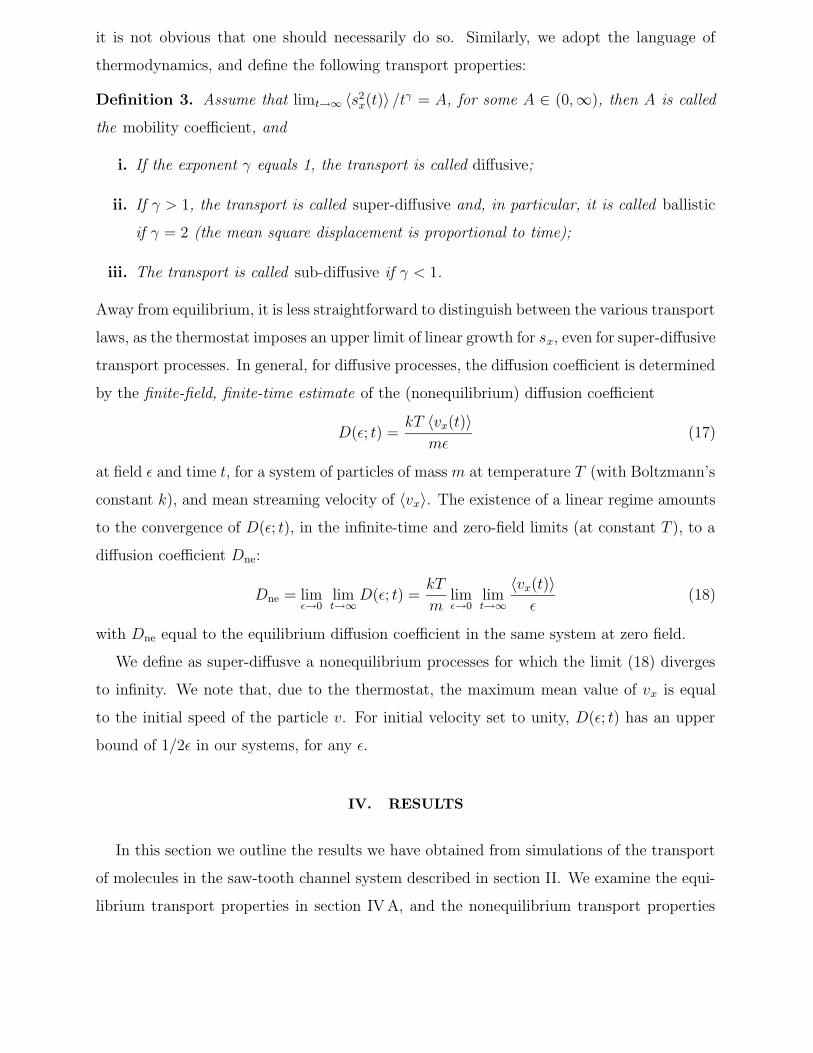
Definition 3. Assume that limt→∞ 〈s2x(t)〉 /tγ = A, for some A ∈ (0,∞), then A is called

the mobility coefficient, and

i. If the exponent γ equals 1, the transport is called diffusive;

ii. If γ > 1, the transport is called super-diffusive and, in particular, it is called ballistic

if γ = 2 (the mean square displacement is proportional to time);

iii. The transport is called sub-diffusive if γ < 1.

Away from equilibrium, it is less straightforward to distinguish between the various transport

laws, as the thermostat imposes an upper limit of linear growth for sx, even for super-diffusive

transport processes. In general, for diffusive processes, the diffusion coefficient is determined

by the finite-field, finite-time estimate of the (nonequilibrium) diffusion coefficient

D(ε; t) =kT 〈vx(t)〉

mε(17)

at field ε and time t, for a system of particles of mass m at temperature T (with Boltzmann’s

constant k), and mean streaming velocity of 〈vx〉. The existence of a linear regime amounts

to the convergence of D(ε; t), in the infinite-time and zero-field limits (at constant T ), to a

diffusion coefficient Dne:

Dne = limε→0

limt→∞

D(ε; t) =kT

mlimε→0

limt→∞〈vx(t)〉ε

(18)

with Dne equal to the equilibrium diffusion coefficient in the same system at zero field.

We define as super-diffusve a nonequilibrium processes for which the limit (18) diverges

to infinity. We note that, due to the thermostat, the maximum mean value of vx is equal

to the initial speed of the particle v. For initial velocity set to unity, D(ε; t) has an upper

bound of 1/2ε in our systems, for any ε.

IV. RESULTS

In this section we outline the results we have obtained from simulations of the transport

of molecules in the saw-tooth channel system described in section II. We examine the equi-

librium transport properties in section IV A, and the nonequilibrium transport properties

12

in section IV B. In both cases, we will be interested in the collective, ensemble behaviour

of particles in the system, and how this ensemble behaviour relates to the behaviour of

individual trajectories.

A. Equilibrium

The ergodic properties of our systems are not obvious, therefore, there seems to be no

immediate choice for a probability distribution in phase space, to be used for the ensemble

averages. Nevertheless, the uniform probability distribution (Lebesgue or Liouville measure,

defined above) is invariant, and one could think that it is appropriate for transport in a

membrane which receives particles from a reservoir, inside which the dynamics is chaotic.

Therefore, the ensemble averages in this section are all computed assigning equal weight to

all regions of phase space.

1. Parallel walls, collective behaviour

In Figure 2 we depict the mean-square displacement, as a function of time, for a series of

parallel saw-tooth systems (∆yt = ∆yb = ∆y). We examine systems where the ratio ∆y/∆x

varies from 0.25 to 3, so that the angle θ = θt = θb the saw-tooth makes with the horizontal

varies from about 0.08π radian (≈ 14◦) to about 0.4π radians (≈ 72◦). Each graph shows

results for a single value of ∆y/∆x, for various pore heights h. For each choice of ∆y

(recalling that ∆x = 0.5), we examined pores with heights h = 1.5∆y, 2∆y, 2.05∆y, 3∆y

and 21∆y. The corresponding interior pore heights are d = 0.5∆y,∆y, 1.05∆y, 2∆y and

20∆y. We note that h = 2∆y corresponds to the critical pore width, above which the

billiard horizon is infinite (i.e. there is no upper bound to the length of possible molecule

trajectory segments without boundary collisions). We considered sets of initial conditions

ranging from 1000 to 5000 particles. For clarity, we do not include the error bars on the

graphs in this or subsequent figures showing the mean square displacement as a function

of time — however, the error estimates obtained have been used in the determination of

the transport law exponents (see below). Not surprisingly, given the clearly non-diffusive

nature of the transport observed in Figure 2, the corresponding super Burnett coefficients

do not appear to have a well-defined value, but diverge over time.

13

The same data have also been generated for a series of systems with one flat wall and one

saw-tooth wall, which always have an infinite horizon. For these systems, we set ∆yt = 0,

and considered the same ratios ∆yb/∆x as were examined in the parallel saw-tooth systems

with pore heights h = 1.05∆yb, 2.5∆yb and 20.5∆yb (which have corresponding interior

heights d = 0.55∆y, 2∆y and 20∆y). Sets of initial conditions ranged from 1000 to 5000

particles. There appeared to be a longer initial transient period for the systems with one flat

wall, but otherwise the results were qualitatively the same as for the parallel wall, despite

the infinite horizon.

Table I shows the values of the exponents obtained from fitting the data in Figure 2 and

those for one flat wall to (16), for both the parallel saw-tooth systems and the systems with

one flat wall and one parallel wall. Data and error estimates in the Table were determined

using a Marquardt-Levenberg non-linear least squares fit of the data and error estimates of

individual points. In all cases, we observe that the transport is significantly super-diffusive,

but not ballistic. For the ∆y/∆x = 1 system, which is a (parallel) rational polygonal

billiard, we observe an exponent γ ≈ 1.65. All other choices of ∆y/∆x represent (parallel)

irrational polygonal billiards. For ∆y/∆x = 1/4 (where θ < π/4), we observe an exponent

of γ ≈ 1.85 in all systems. For ∆y/∆x = 2 and ∆y/∆x = 3 (where θ > π/4), we observe

a similar exponent in the systems with pore height less than or in the vicinity of 2∆y, and

a reduction in the transport exponent as the pore height increases (a corrugation effect).

The same value γ ≈ 1.85 has been found by M. Falcioni and A.Vulpiani in the equilibrium

version of the periodic Ehrenfest gas of Ref.[17], [34].

We have also examined the distribution of the total x displacements sx(t), as a function

of time. Distributions for the ∆y/∆x = 1 system (obtained from 2000 initial conditions)

and the ∆y/∆x = 2 system (obtained from 5000 initial conditions), obtained at the end of

the simulations, are shown in Figure 3. The results for the ∆y/∆x = 2 system are typical of

the results observed for the other parallel irrational polygonal billiards. Errors are estimated

from the frequency counts used to generate the histograms.

From an initial distribution that is effectively a delta function on the scale of the motion,

the transport process produces symmetric distributions, distinct from a Gaussian distribu-

tion. For the parallel irrational polygonal billiards, the distribution appears Gaussian out

to one standard deviation — however, the distribution at larger displacements is clearly

underestimated by the Gaussian. Attempted fits using functions of the form exp{−xα} fail

14

to capture the shape both at the centre and in the tails, although the tails appear to be well

modelled by a distribution of the form exp{−x1.4} (Figure 3a). When θ = π/4, however, the

distribution bears little resemblance to a Gaussian (Figure 3b). Analogous results in each

case were obtained from the systems with one flat wall and one saw-tooth wall.

We have also examined the behaviour of the momenta of particles in our systems. Given

that the speed is preserved by the dynamics, the momenta can vary only in orientation, and

we therefore examine the effect of the dynamics on the distribution of these orientations.

Figure 4 shows the typical behaviour of the distribution of momenta orientations at the

beginning, at the midpoint, and at the end of a typical simulation of 5000 particles. We also

show a mean distribution obtained from averaging the momentum data over all sampled

times, as well as over all trajectories. We find that there are no significant correlations

in the distributions of the momenta over the course of the simulation. The distribution

of orientations does not converge to the uniform distribution over the time-scales we have

considered (as we might expect it to for a large system of interacting particles): nor does it

appear to diverge further from the uniform distribution. Any memory effects do not appear

to have a significant influence on the overall distribution at any instant. Again, the same

conclusions can be drawn from similar examination of the systems with one flat wall and

one saw-tooth wall.

Remark 1. The dependence of the transport law on the angles θi, but not on the pore

height, is remiscent of the behaviour in (chaotically) dispersing billiards. There, the infinite

horizon adds a logarithmic correction to the time dependence of mean square displacement,

which is hard to detect numerically. Despite the lack of chaos, our non-dispersing billiards

could display similar logarithmic corrections when the horizon is infinite [20].

More surprising is the observation that in some cases the overall mass transport decreases

as the pore width increases while the horizon is finite, and only increases again once the

horizon is infinite.

2. Parallel walls, individual behaviours

From the results we have obtained, there appear to be well-defined collective behaviours

that are attributable to the systems we have studied — that is to say, the mean values of

the properties obtained from simulation appear to converge, in the limit of a large number

15

of independent trajectories (or particles), to well-defined values. In analogy to what we have

presented above, we examine the evolution of the individual particle momenta, and the x

displacements.

The picture of the momenta is trivial in the ∆y/∆x = 1 systems, because for θ = π/4

only four orientations per trajectory at most are possible, as determined by the initial

condition. The picture of the momenta for irrational systems appears less predictable. Over

the course of the simulations, sequences of momenta, sampled at intervals of 104 time units,

were collected. In Figure 5 we show such a sequence of momenta, sampled from a system

where ∆y/∆x = 3, accumulated up to the 5 × 105 time units (Figure 5a), 2 × 106 time

units (Figure 5b), and 107 time units (Figure 5c). The momenta are represented by symbols

(circles) on the unit circle IT 1, while the lines indicate the sequence of the sampled momenta.

It is clear from Figure 5 that, despite consisting of up to 1000 different sampled momenta,

the number of distinct momenta visited by the particle is relatively small (of the order of

10-20). Furthermore, the growth of this set is gradual, and strongly correlated to the set of

momenta that precede it in the sequence of momenta visited by the particle. The choice of

θ irrationally related to π permits, in principle, the exploration of the whole unit circle of

orientations. However, it is clear that the nature of the sequence of wall collisions limits the

rate at which such an exploration of the unit circle can be achieved. This slow growth was

observed for simulation times up to 109 time units (not shown here).

In Figure 6 we show the sequence of the first 1000 momenta, sampled every 104 time units,

for six distinct initial conditions in a ∆y/∆x = 3 system. In each case, the available velocity

phase space is gradually explored by the particle. We note that the rate and manner in which

this exploration takes place (as indicated by the lines joining consecutive sample momenta)

depends significantly, and unpredictably, on the initial condition, as is demonstrated by

the visibly different structures generated by each. This feature is common to all parallel

irrational polygonal billiards examined — for systems with parallel saw-tooth walls and

systems with one flat wall and one saw-tooth wall. The flat wall in these latter systems

induces a vertical symmetry that is absent in the parallel systems, and appears to increase

the range of momenta visited by particles — however, a similar degree of connectivity is

observed in both cases.

Finally, we turn our attention to the behaviour of the displacements sx(t) for individual

initial conditions, as a function of time, which we expect to give further insight into the

16

manner in which the momentum space is explored. In Figure 7, we show sx(t) as a function

of time over four different time-scales for a single particle trajectory in a system where

∆y/∆x = 0.25. Again, such a trajectory is typical of the results observed for the parallel

irrational polygonal billiards examined. In Figure 8, we show an analogous set of results for

transport of a particle in a (rational) θ = π/4 system.

In Figure 7a, the dynamics appear somewhat random on the scale of 106 time units,

although on closer inspection it is clear that certain sections of the trajectory are repeated.

Indeed, the occurrence of repeated segments is more obvious in Figure 7b, where after

an initial transience of 106 steps, the simulation appears to reach a periodic orbit, before

changing to another orbit in the interval at about 3.5×106, then reverting to the original

orbit at around 8×106 time units. On a longer time scale (Figure 7c), the transport appears

to alternate between these two almost periodic orbits. However, on the scale of 109 time units

(Figure 7d), the evolution of sx takes on quite a different appearance, bearing a similarity

with what one might observe for the random motion of a particle in a low-density gas. Such

a resemblance suggests that, on this time-scale, there could be sufficient memory loss of

the preceding momentum values for the trajectory to appear random. Even at this stage,

however, the number of distinct momenta visited by the particle is still limited to the order

to 10-100.

To give some physical sense to these observations, we consider the analogy of the transport

of a light gas (such as methane) along a nanopore of width 1 nm. At room temperature,

the unit velocity in our particle corresponds to a root-mean-square velocity for methane of

approximately 400 m/s. It follows that our time units correspond to the order of picoseconds.

Thus, for the system above, the correlation length in is about 109 ps = 1 µs, during which

the particle will have a net displacement along the pore of the order of millimetres. We note

that the mean inter-molecular collision time would be much less than this, for all but the

most rarified of conditions.

In contrast, we recall that the transport behaviour in the θ = π/4 system is restricted

to a maximum of four distinct momenta, for each initial condition. Despite this apparently

strong limitation, a richness in behaviour is still evident. In Figure 8, we observe strongly

recurrent behaviour on all time-scales observed, although the nature of the recurrence varies

on all observed time-scales, and is likely to continue to do so at larger and larger scales. We

note that Figure 7d and Figure 8c represent the evolution of sx over the same time-length

17

— however, while this evolution appears random in the irrational system, the motion is

regular in the rational case. The regularity is less trivial in Figure 8d, with four small steps

between the first two large steps, but only three small steps between the second two large

steps, showing that the apparent regularity doesn’t make the dynamics easily predictable.

Continuing the physical analogy above, the lower bound for the correlation time in this

system is closer to the order of seconds, although the mean displacement over this time is

still of the order of millimetres (because of the slower transport, reflected by the smaller

value of γ).

In Figure 9a, we show the distribution of displacements obtained by dividing the 109 time-

unit trajectory for the ∆y/∆x = 0.25 system into segments of shorter time periods, in order

to compare with the approximation to the ensemble distribution obtained from averaging

over trajectories with independent initial conditions. It is clear from the figure that the

two distributions are significantly different — while the ensemble distribution demonstrates

the near-Gaussian properties observed earlier, the distribution from the single trajectory is

significantly skewed (as could be expected from Figure 7), and has a distribution that is

much narrower than that of the ensemble. The correlations observed along the trajectory

in Figure 7 lead to a distribution of displacements that is not at all characteristic of the

ensemble, up to a time of one billion time units.

In Figure 9b, we show the distribution of displacements obtained by dividing the 1010

time-unit trajectory for the ∆y/∆x = 1 system into segments, as done above. In constrast

with the results for the ∆y/∆x = 0.25 system, the distribution obtained in this fashion

shows excellent agreement with ensemble distribution of trajectories.

Remark 2. The overall transport is ultimately slower in the rational systems than in the

irrational systems. Furthermore, despite the limitations on the velocities that each single

trajectory can take, which differ from trajectory to trajectory, the distributions of displace-

ments exhibited by one rational trajectory equals the distribution of the ensemble, while this

is not the case for the irrational trajectories !

3. Unparallel walls, collective behaviours

We have examined the transport properties of a series of unparallel saw-tooth systems,

chosen such that the ratios ∆yb/∆x lie in the vicinity of the golden ratio (√

5+1)/2 ≈ 1.618,

18

so as to “maximise” the irrationality of the relationship of θ to π. In Figure 10 we show

the behaviour of the mean-square displacement, and the estimated diffusion coefficient, as

a function of time, for a series of unparallel saw-tooth systems where ∆x = 0.5,∆yt/∆x =

0.62, and ∆yb/∆x = 0.65. In analogy to the results above, we have examined these systems

at the same range of pore heights based on the mean interior pore height dc = (∆yt+∆yb)/2

at which the horizon becomes infinite — at d = 0.5dc, dc, 1.05dc, 2dc and 20dc.

Despite containing data from 10000 independent initial conditions, the data in Figure 10

exhibit features suggesting that they have not yet converged to a final result. These features

correspond to significant jumps in the mean-squared displacements (and consequently the

finite-time estimate of the diffusion coefficient), resulting from short bursts of quasi-periodic

behaviour (i.e. ballistic transport). We note from Figure 10 that the effects of the bursts

appears to grow as the horizon is opened. Similar jumps are observed in the time-evolution

of the super Burnett coefficients, indicating that the bursts contribute to driving the system

away from a Gaussian distribution.

To give some sense of the size and frequency of these bursts, we show the distribution

of displacements obtained over intervals of 105 time units, combining contributions from

all 104 initial conditions, in Figure 11. We observe excellent agreement with the Gaussian

distribution, out to several standard deviations. However, in the tail of the distribution we

find a non-negligible contribution from large-scale displacements, to which we attribute the

behaviour of the super Burnett coefficients. These contributions correspond to the bursts

observed in Figure 10, and it is clear that a huge number of initial conditions would be

required before the overall effect of this tail distribution could be realised by simulation.

Table II shows the values of the exponents obtained from fitting the data from the ob-

served systems to (16), and obtain behaviour that is close to diffusive. The significant errors

in the data arise from the ballistic bursts, so that a least-squares error estimate, more appro-

priate for random errors, may not be as appropriate here. However, the least-squares error

estimates still provide useful information regarding the relative errors in the data obtained

for the various systems.

From Figure 11 it is clear that the bursts only occur for a small number of particles. We

have found that, in each case, only 2 or 3 initial conditions are responsible for the ‘significant’

bursts — that is to say, if the contribution from these 2 or 3 particles (in 10000) is neglected,

the resultant behaviour is diffusive within statistical error, and the fluctuations all lie within

19

error about this mean diffusive behaviour. Within statistical error, one could conjecture

that the effect of these ‘significant’ bursts is not sufficient to drive the behaviour away

from diffusive behaviour, given the decay back to diffusive transport observed in Figure 10

after each burst. Clearly, however, it cannot be excluded that the effect of these bursts is

to drive the transport at a rate somewhat faster than diffusive, either with an exponent

slightly greater than 1, or with some slower correction, such as the ln t correction for the

Sinai billiard. This correction has been the subject of recent studies for polygonal channel

transport [20]. We note, with the Sinai billiard in mind, that the bursts responsible for this

potentially super-diffusive behaviour are observed in systems with both open and closed

horizons.

In Figure 12, we show the distribution of displacements after 106 time units, and after

107 time units, from the trajectories of individual particles, again noting that the initial

distribution is effectively a delta function since all particles begin from the same unit cell

at sx = 0. Even after 106 time units, the distribution of displacements is very well fit by a

Gaussian, consistent with our observations of a diffusive transport rate, and in contrast to

the results for the parallel walls.

As with the case of parallel walls, the momenta do not appear to be significantly correlated

over the course of the simulation, and there is stronger evidence in this case of a convergence

to a uniform distribution than in the parallel case.

4. Unparallel walls, individual behaviours

As with the parallel systems, we have considered the behaviour along longer individual

trajectories, to compare with the ensemble behaviour. For unparallel walls, we find that

there is strong agreement between the individual and ensemble behaviours, in terms of the

distribution of both the momentum orientations and of the displacements. Sequences of

momenta appear random along a trajectory, and the distribution of displacements obtained

along a single trajectory demonstrates an excellent Gaussian fit, in agreement with the

ensemble results.

20

B. Nonequilibrium

An alternative method of studying the transport behaviour is to consider the dynamics

in the presence of an external field. For thermodynamic fluids, we expect that the transport

coefficient determined in the linear response regime (i.e. in the zero-field limit) for the

nonequilibrium fluid corresponds to that obtained from the equilibrium fluid properties. It

is not clear, a priori, that such an equivalence holds for the system examined in this paper,

so we examine the nonequilibrium transport properties, as a dynamical system of interest in

its own right, as well as to compare its behaviour with that of the equilibrium counterpart.

1. Parallel

For the non-zero-field estimates of the transport coefficient for the ∆y = 2 system, with

d = 0.5∆y, for the four different field strenghts ε = 0.1, 0.01, 10−3, 10−4, we find that the

qualitative behaviour of the particles is highly, and unpredictably, dependent on the field

strength. At the highest field, ε = 0.1, (Figure 13a) all trajectories have similar qualitative

and quantitative properties, demonstrating a “fluid-like” response to the external field —

particles are driven in the direction of the field, and the fluctuations about a mean transport

rate are small, since the field is strong. At ε = 0.01, however, the trajectories exhibit two

distinct transport phases — an initial phase where the particle trajectories fluctuate about a

mean motion due to the driving field, and a second ballistic phase, where the trajectory finds

a periodic orbit (Figure 13b). At this field, two distinct orbits were noted — one consisting

of 33 reflections, with period τ = 9.6950889... and mean net speed vb ≈ 0.31, the other

consisting of 39 reflections, with period τ = 12.393386... and mean net speed of vb ≈ 0.24.

The orbits are shown in Figure 14. In particular, we note the existence of distinct periodic

orbits to which the different trajectories converge, demonstrating that the dynamics at this

field strength is not ergodic. At lower fields, a transition to periodic orbits is much rarer

— however, bursts of almost-periodic orbits are observed, which decay after relatively short

times to revert to the previous apparently random behaviour (Figure 13d).

This transition from apparently random transport to ballistic transport has been observed

previously in a similar nonequilibrium system with straight walls [17]. There, a transition

time was observed between these two transport behaviours, which varied as the inverse

21

square of the external field strength. Our results appear to be consistent with such a rela-

tionship, inasmuch as the fraction of observed periodic orbits (indicating ballistic transport)

decreases as the field strength increases. We expect that longer simulations would produce

a larger fraction of such periodic orbits, and suggest that the reason we do not observe any

ballistic transport in the weakest field is due to the much larger time-scale on which such a

transition would take place. Unlike the systems in [17], where only the ensemble behaviour

was studied, and a smooth transition from diffusive to ballistic transport was observed at fi-

nite times, here we consider the single trajectories, and find that their individual transitions

are sharp and occur apparently at times not limited by any upper bound.

We show the estimates of D(ε; t) for the applied fields ε for the parallel ∆y/∆x = 2

system in Column 2 of Table III. Over such a range of fields, we would expect to observe

either convergence to a well-defined value (the diffusion coefficient), or divergent behaviour

(bounded by the thermostat). However, we note that D(ε; t) does not diverge in the zero-

field limit, as we would expect for a real fluid which exhibited superdiffusive equilibrium

behaviour (such as plug flow).

2. Non-parallel

In contrast to the results for the parallel systems, we find that the individual particle

trajectories for the ∆yt/∆x = 0.62,∆yb/∆x = 0.65, d = 0.5dc system display the same char-

acteristic behaviour for the four different field strengths ε = 0.1, 0.01, 10−3, 10−4 examined.

Trajectories are typified by an initial apparently random transient behaviour, followed by a

transition to ballistic transport in a periodic orbit. The transition time also appears to vary

inversely with the field strength. As a consequence, the fraction of trajectories observed to

undergo a transition within 106 time units decreases with decreasing field, and therefore the

lifetime of the non-ballisitic regime grows.

These results are consistent with those of Ref.[17], which were obtained using parallel

boundary walls, where the wall angles were chosen such that tan θ was close to the golden

ratio. It is possible that such a choice leads to much smaller correlation times in the mo-

mentum sequence for particle trajectories, and consequently faster convergence to the longer

time-scale behaviour more reminiscent of intermolecular collisions, observed in Figure 7.

For a given field strength ε, each ballistic trajectory appears to have the same mean net

22

speed. For each field strength considered, this mean net speed appears to be vb ≈ 0.48. We

find that the individual trajectories converge to a single periodic orbit that is independent

of the initial conditions, but dependent on the field strength. These orbits are shown in

Figure 15. We note that these periodic orbits appear to be instances of a continuous family

of periodic orbits, converging to a limiting orbit in the zero-field limit. However, this limiting

orbit is never observed in the equilibrium trajectories, where it is no longer an attractor.

The existence of a family of attractive periodic orbits, converging to a precise periodic

orbit in the zero-field limit, precludes the existence of a linear regime, and is significantly

at odds with what one would expect of an ergodic, diffusive system in nonequilibrium.

For such systems, we would anticipate the convergence of the nonequilibrium finite-field

estimates D(ε; t) to the equilibrium value D in the zero-field, infinite-time limit. However,

the limiting periodic orbit with a finite net speed vb ≈ 0.48 implies that the finite-field,

finite-time estimate D(ε; t) must diverge as the field goes to zero.

However, as noted above, the fraction of trajectories that turn ballistic within a given time

t decreases with decreasing field, so that in the ε→ 0 limit we expect this fraction to tend to

0. Furthermore, the behaviour of the trajectories before they reach a periodic orbit remains

apparently random, and responsive to the field. Consequently, we consider the following

approach to constructing the “weak” linear regime. At any given time, we neglect those

trajectories already captured by a periodic orbit (ie whose transport has become ballistic),

and we define a finite diffusion coefficient based upon the remaining trajectories. Usually,

one defines the nonequilibrium diffusion coefficient (following the Green-Kubo result (18))

by taking the limits t→ 0 and ε→ 0 separately — here, this is no longer possible if we wish

to avoid periodic trajectories, so the limits must be taken simultaneously.

Therefore, given a sufficiently large ensemble of N particles, assume that the fraction

ν(ε; t) of particles which are still in the diffusive regime, at time t and for field strength ε,

is well-defined. Let M(N ; ε; t) be the subset of indices in {1, . . . , N} of these still-diffusive

trajectories. Assume that for every δ > 0 there is a field εδ > 0 such that ν(ε; t) ≥ 1 − δ if

ε < εδ and N is sufficiently large, as seems to be the case in our simulations. For simplicity,

assume that there is a function ε = ε(t; δ), such that ν(ε(t; δ); t) = 1 − δ/2. Finally, define

N(δ) = [2l/δ], where [·] represents the integer part, and choose integer l so large that N(δ)

is sufficiently large for the fraction δ/2 to be sufficiently finely realized, for any δ > 0.

23

Definition 4. For every δ > 0, distribute at random (with respect to the Lebesgue measure)

N(δ) initial conditions in the phase space. For each of them and for fixed t, consider

D∗i (ε; t) =kTvi,x(t)

mε, i ∈ {1, . . . , N} ,

where vi,x(t) is the mean x-component of the velocity of the i-th trajectory at time t (and other

variables defined as in (17)). The weak nonequilibrium estimate of the diffusion coefficient,

if it exists, is defined by

D∗ne = limδ→0

limt→∞

1

N(δ)ν(ε(t; δ); t)

∑

i∈M(N(δ);ε;t)

D∗i (ε(t; δ); t)

= limδ→0

limt→∞

kT

mε(t; δ)

1

N(δ)ν(ε(t; δ); t)

1

t

∑

i∈M(N(δ);ε;t)

sxi(t),

(19)

Thus, for a given choice of δ, and t, we evaluate the estimate of the diffusion coefficient

(17) considering only those trajectories which have not been captured by a periodic orbit.

Then, the limit t→∞ includes also the limit ε→ 0, and the limit δ → 0 includes the limit

N →∞. We can now define the following:

Definition 5. If the equilibrium system has a finite diffusion coefficient D, and D∗ne = D,

the system is said to have a weak linear regime.

In Table III we report the ‘corrected’ estimates D∗(ε; t) for the various fields, where we

neglect contributions from ballistic trajectories. In the third column we report estimates

for the parallel ∆y/∆x = 2 system, and in the fifth column we report estimates for the

unparallel ∆yt/∆x = 0.62,∆yb/∆x = 0.65, d = 0.5dc system. We note that the ‘corrected’

data for the parallel ∆y/∆x = 2 system are consistent with a divergent trend (taking

into account the large statistical error in the weakest field). For the unparallel system, the

equilibrium and nonequilibrium transport properties become more consistent, although they

are not conclusively so, because of the large error bars produced by the statistical analysis at

low field. Such noise is typical of NEMD simulations at low field, where the signal-to-noise

ratio becomes low. Typical NEMD simulations, however, would still converge to yield the

same transport coefficient in the long-time limit — in our non-chaotic systems, the transition

from random to ballistic behaviour effectively places an upper bound on the time during

which random behaviour can be observed. The estimated errors in the diffusion coefficient

obtained will therefore depend on the rate at which the mean transition time increases with

decreasing field.

24

Remark 3. This subsection leads us to conclude that the use of thermostats needs some

form of chaos, whether permanent or transient, in order for a linear regime to be observed.

This is a cause for concern in the case of thermostatted non-interacting particle systems.

V. TRANSPORT COMPLEXITY

As we have seen, the transport properties of the dynamics in these systems we have

studied are strongly dependent on the angles θi. Dependence of thermodynamic properties

on the boundary geometry is a well-studied phenomenon in models of porous media, or

systems which resemble them. For certain chaotic dynamical systems of non-interacting

particles, these thermodynamic properties are known to vary irregularly as a function of

boundary parameters [23–27]. However, all of these systems exhibit diffusive transport,

irrespective of the variation of the diffusion coefficient. By contrast, the transport processes

of the non-chaotic systems in this paper demonstrate an unpredictability of the exponent γ

determining the transport law, as well as of the corresponding mobility coefficient.

It would therefore seem that the non-chaotic transport studied in this paper is, in some

sense, more unpredictable than transport in their chaotic counterparts, and thus more com-

plex [35]. This conceptual connection between unpredictability and complexity can be un-

derstood through the perspective of information theory. The unpredictability of a system

is related to the information required to describe the system state — less predictable sys-

tems require more information to describe them, and can therefore be interpreted as more

complex. Studies of the complexity of polygonal billiards already appear in the literature,

based on the symbolic dynamics of particle trajectories. In such studies, the growth of the

number of permitted “symbolic trajectories” with trajectory length gives a measure of the

complexity of the system.

In chaotic systems, nearby trajectories separate at an exponential rate in phase space,

and the symbolic dynamics of such systems admits a range of “symbolic trajectories” that

grows exponentially with the trajectory length. However, while non-chaotic systems can

also exhibit a sensitivity to initial conditions, nearby trajectories do not separate at an

exponential rate in phase space, and the number of allowed “symbolic trajectories” grows

sub-exponentially [21]. From this microscopic measure of complexity, one would conclude

that the chaotic systems are more complex than the non-chaotic systems — a conclusion

25

that seems in complete contradiction to the observed macroscopic behaviour.

It is precisely at this distinction between microscopic and macroscopic behaviour that

the apparent contradiction arises. The mixing properties of chaotic dynamics causes almost

all trajectories to have the same macroscopic properties. If there are super-diffusive or

sub-diffusive trajectories permitted over finite symbolic trajectories, the proportion of such

trajectories, compared with all allowed trajectories, must go to zero in the infinite-time

limit. If all but a negligible set of trajectories are diffusive in this limit, then the only

possible variation (and hence unpredictability) in the transport process must be at the level

of the mobility coefficient. In the non-chaotic case, diffusive trajectories do not always

dominate the set of allowed trajectories in the large time limit, and the unpredictability

of the transport processes extends to the exponent γ as well as to the mobility coefficient.

We believe that it is of great significance to note that the measure of complexity at the

microscopic level does not reflect the unpredictability of the transport properties we are

interested in at the macroscopic level.

Other non-chaotic maps have been observed to demonstrate a similar class of complexity

as those in this paper — see Ref.[36] (where the geometry unpredictably gave periodic, dif-

fusive or ballistic behaviour) and Ref.[37]. Our numerical results indicate that the transport

law can change from diffusive to sub-diffusive regimes, or alternatively quite high superdif-

fusive regimes, after small changes of the parameters defining the geometry. To quantify

this kind of complexity, we propose the following definitions.

Definition 6. Consider a transport model, whose geometry is determined by the parameter

y, which ranges in the interval [0, h], and such that its transport law is given by

limt→∞〈s2x(t)〉tγ

= A , 0 < A <∞ (20)

with γ a function of y varying in [0, 2], when y spans [0, h]. Let ∆γ(ym, yM) ∈ [0,∞]

be the difference between the largest and the smallest value of γ, for y in the subinterval

(ym, yM ) ⊂ [0, h], where ∆γ(ym, yM ) = ∞ if in (ym, yM) there are points for which (20) is

not satisfied by any γ ≥ 0.

i. The transport complexity of first kind of the transport model in (ym, yM ) is the number

C1(ym, yM ) =h∆γ(ym, yM )

2(yM − ym)∈ [0,∞) (21)

if it exists.

26

ii. The transport complexity of second kind of the transport model for y = y is the

exponent C2 = C2(y), if it exists, for which the limit

limε→0

C1(y − ε, y + ε)

εC2(y)(22)

is finite.

iii. The transport complexity of third kind of the transport model for y = y is the limit

C3(y) = limε→0

∆γ(y − ε, y + ε) (23)

These definitions are motivated by the following considerations. If C1 does not vanish, the

system is surely highly unpredictable from the point of view of transport, in the interval

(ym, yM ), because its transport law is only known with a given uncertainty. This could

be the case, for instance, of a batch of microporous membranes with flat pore walls, whose

orientation is obtained with a certain tolerance (transport complexity of first kind). However,

C1 may diverge around some point of [0, h], as our data seem to indicate, giving rise to an

even higher level of transport complexity. Assuming that this divergence has the form of a

power law, we take the power as a measure of this second kind of complexity. But even this

level of complexity seems to be insufficient for our models, which indicate that ∆γ(ym, yM )

could be discontinuous. For this reason, we introduce the third kind of transport complexity.

In order to further investigate these notions, and how they relate to our systems, we have

considered the transport behaviour in a narrow range about two principal systems, taken

from the examples of super-diffusive transport observed in Section IV A. The first principal

system is the rational parallel ∆yt/∆x = 1, where we consider the transport behaviour in

the limit that ∆yb/∆x → 1,∆yb/∆x > 1. The second principal system is the irrational

parallel ∆yt/∆x = 2 system, where we consider the transport behaviour in the limit that

∆yb/∆x→ 2,∆yb/∆x > 2. In Table IV, we show the exponent γ of the transport laws (as

per (20)) corresponding to the various choices for ∆yt and ∆yb.

We note that, in both cases, there appears to be a strong discontinuity at ∆yt = ∆yb —

when the walls are not parallel, the behaviour is no longer superdiffusive. In the rational

case, the transport coefficient appears to depend unpredictably on the ∆yt, but is always

distinctly sub-diffusive. By contrast, in the irrational case, the transport appears to be

essentially diffusive when the walls are not parallel. This behaviour is consistent with that

observed in Section IV A 3 for the unparallel walls, which are also irrational.

27

Due to the discontinuity, the transport complexities C1 and C2 diverge in these cases,

reflecting the high degree of unpredictability that has been observed in the previous sections,

which can only be quantified by C3.

VI. CONCLUSION

In this paper, we have examined the transport properties of a dynamical system of re-

markable simplicity — a two-dimensional channel with straight-edged walls, populated by

non-interacting, point-like particles. In spite of the absence of dynamical chaos, this system

displays a rich variety of transport behaviours.

In the equilibrium systems, we observe sub-diffusive, diffusve, and super-diffusive trans-

port (although no ballistic behaviour). This behaviour is strongly dependent on the angles

θi, and only weakly dependent on the pore height. The opening of the horizon appears to en-

courage super-diffusive “bursts” in the diffusive systems, possibly inducing a time-dependent

divergence of the diffusion coefficient. In the super-diffusive systems, opening the horizon

appears to reduce the exponent γ, although the overall mass transport is greater. This result

suggests that wall reflections lead to greater randomness in wider pores, where the dynamics

resembles transport along a corrugated channel, and that the sequence of wall collisions is

less restricted than in the narrower pores, leading to slower, more diffusive transport. Also

in the parallel systems, we note the curious phenomenon whereby the transport coefficient

appears to increase as the pore width is decreased, once the horizon has been closed.

The difference in behaviour of trajectories in the diffusive and super-diffusve systems

is clear, in terms of the correlation of successive momenta. In the diffusve systems these

correlations die off quickly, whereas they produce quasi-periodic “building blocks” in the

super-diffusve trajectories, observable on various length scales. Despite these correlations,

the trajectory behaviour is seemingly unpredictable from one order of magnitude of time

to the next. While parallel systems with irrational θ can in principle access the whole

momentum space, it is only on the scale of some 1010 time units that apparently random

behaviour is observed. This raises the interesting possibility that the behaviour could indeed

become diffusive on longer trajectories, but only on such (computationally expensive) time

scales. There is no evidence on the time scales studied of such a possibility for the rational

system, which is a reflection of the finite number of distinct momenta accessible along a

28

single trajectory in such systems.

In no case have we observed nonequilibrium transport behaviour that appears to cor-

respond to the associated equilibrium system. In the case of super-diffusive behaviour at

equilibrium, one would expect the finite-field diffusion coefficients to diverge in the limit of

zero field. Such a divergence would have an upper bound inversely proportional to the field

strength. For the systems which are diffusive at equilibrium, we would expect the finite-field

estimates to converge to the equilibrium diffusion coefficient. Instead, we find that the finite

field estimates do not clearly diverge for the systems that are super-diffusive at equilibrium,

and that they clearly do diverge for systems that are diffusve at equilibrium, due to the

existence of attractive periodic orbits.

For the nonequilibrium parallel systems, the existence of and convergence towards peri-

odic orbits appears irregularly determined by the field strength. We observe clearly non-

ergodic behaviour for one field strength, with the existence of distinct attractive periodic

trajectories for a single dynamical system. For the nonequilibrium unparallel systems, there

is a much more regular field-dependence of the transport behaviour. Each trajectory con-

verges toward a periodic orbit which is unique for a given field (and appears to be contin-

uously dependent on the field), and the mean onset time of the periodic orbit grows with

decreasing field strength.

Importantly, we note that the absense of clear “thermodynamic” behaviour tends to

support the existing CH, such as those in Ref.[3]. Interestingly, however, there appears to

be the possibility of a weak linear regime, before the onset of the periodic behaviour in

the unparallel systems. This approach requires the alternative definition of a “weak” linear

regime, using a non-standard order of the time and field-strength limits. Our results on the

existence of this “weak” linear regime and its thermodynamic interpration are unclear, and

are a source of on-going research.

The range of transport behaviours we have observed, and their unpredictability, raise an

interesting contradiction with regards to existing methods for quantifying the complexity

of a system. These existing methods focus on the application of information theory at

the microscopic level, to determine the unpredictablility, and thus the complexity, of the

microscopic behaviour. Such an approach would suggest that chaotic systems should be more

complex than unchaotic systems — an interpretation that seems intuitively at odds with

the behaviour of macroscopic properties such as the overall transport. The reason for this

29

contradiction lies in the fact that, while the chaotic system can exhibit a greater “diversity”

of trajectories than the non-chaotic systems at the microscopic level, they correspond to

a smaller “diversity” of overall transport behaviours. It is this diversity with respect to a

particular macroscopic property of interest that we aim to incorporate in our quantification

of transport complexity. More complicated notions of transport complexity may then be

envisaged, but the conceptual picture outlined here would not change. We note that there

may be some degree of subjectivity to our definition of transport complexity, to the extent

that we consider “diversity” with respect to a particular property. This aspect of our notions

is one avenue of further investigation.

We note that, for the sake of simplicity, we have focussed on the dependence of the

transport law on just one paramenter, but our investigation reveals that transport in our

models may depend in a counterintuitive and irregular fashion on other parameters as well,

such as pore height. We anticipate that these notions will be useful in distinguishing between

various transport systems, with reference to the diversity of transport properties that they

exhibit, and in particular the predictability of these transport properties. For example,

slight differences in the manufacturing of porous membranes may result in totally different

transport properties.

This analysis leads us to the following observation. As is well known, the thermody-

namical properties of a macroscopic system are not a function of the system boundary; the

nature of transport, and the transport properties of a fluid, are essentially independent of

the geometry of its container. Fermi expressed this concept, at the beginning of his book

on thermodynamics [38]: “The geometry of our system is obviously characterized not only

by its volume, but also its shape. However, most thermodynamical properties are largely

independent of the shape, and, therefore, the volume is the only geometrical datum that is

ordinarily given. It is only in the cases for which the ratio of surface to volume is very

large (for example, a finely grained substance) that the surface must be considered. This is

clearly understood in the terms of kinetic theory, which leads to explicit expressions for the

diffusion coefficients in terms of only the mean-free paths λ for collisions among particles,

without any reference to the shape of the container. Only in the case that λ is of the same

order of the characteristic lengths of the container, does this play a role; but in that case,

the standard laws of thermodynamics cease to hold, and are replaced by those of highly

rarefied gases, or Knudsen gases [32, 39, 40]. Since our results do not display significant

30

dependence on the surface-volume ratio, they indicate that our systems cannot be consid-

ered as thermodynamic systems, much as they remain highly interesting and important from

both theoretical and technological standpoints. Indeed, as has been noted elsewhere [41, 42],

much care must be taken in the thermodynamic interpretation of the collective behaviour

of systems of non-interacting particles. The arguments of Refs.[41, 42] mainly referred to

nonequilibrium systems: here we provide some examples which show that they apply to

equilibrium systems as well. All this can be summarized stating that a certain degree of

chaos, or of randomness is required in the microscopic dynamics of particle systems, for them

to look like thermodynamic systems, but there are two ways in which this can be achieved.

If the randomness is intrinsic to the fluid, the geometry of the system is a secondary issue,

and the fluid behaves as a proper thermodynamic system. If the randomness is produced

by the geometry of the outer environment, the geometry plays an obviously important role,

and systems such as ours do not behave like proper thermodynamic systems.

VII. ACKNOWLEDGEMENTS

We would like to thank R. Artuso, F. Cecconi, M. Falcioni, R. Klages, A. Lesne and A.

Vulpiani for helpful feedback from preliminary drafts. We would also like to thank the ISI

Foundation for financial support throughout this work.

[1] A.I. Khinchin. Mathematical foundations of statistical mechanics. Dover Publications, New

York, 1949.

[2] G. Gallavotti. Statistical mechanics, a short treatise. Springer-Verlag, Berlin, 1999.

[3] G. Gallavotti and E.G.D. Cohen. Dynamical ensembles in stationary states. Journal of

Statistical Physics, 80(5/6):931, 1995.

[4] P. Gaspard. Chaos, scattering and statistical mechanics. Cambridege University Press, Cam-

bridge, 1998.

[5] D.J. Evans, D.J. Searles, and L. Rondoni. Application of the gallavotti-cohen fluctuation

relation to thermostated steady states near equilibrium. Physical Review E, 71:056120, 2005.

[6] B. Li, G. Casati, and J. Wang. Heat conductivity in linear mixing systems. Physical Review

31

E, 67:021204, 2003.

[7] D. Alonso, A. Ruiz, and I. de Vega. Transport in polygonal billiards. Physica D, 187:184,

2004.

[8] R. Artuso, G. Casati, and I. Guarneri. Numerical study on ergodic properties of triangular

billiards. Physical Review E, 55:6384, 1997.

[9] G. Casati and T. Prosen. Mixing properties of triangular billiards. Physical Review Letters,

83:4729, 1999.

[10] E. Gutkin. Billiard dynamics: a survey with the emphasis on open problems. Regular and

chaotic dynamics, 8(1):1, 2003.

[11] R. Artuso and G. Cristadoro. Weak chaos and anomalous transport: a deterministic approach.

Communications in Nonlinear Science and Numerical Simulations, 8:137, 2003.

[12] Roberto Artuso. Anomalous diffusion in classical dynamical systems. Physics Reports, 290:37–

47, 1997.

[13] E. Gutkin Billiards in polygons Physica D 19:311, 1986.

[14] G. Galerpin, T. Kruger, and S. Troubetzkoy. Local instability of orbits in polygonal and

polyhedral billiards. Communications in Mathematical Physics, 169:463, 1995.

[15] F. Cecconi, D. Castillo-Negrete, M. Falcioni, and A. Vulpiani. The origin of diffusion: the

case of non-chaotic systems. Physica D, 180:129, 2003.

[16] C.P. Dettmann, E.G.D. Cohen, and H. van Beijeren. Microscopic chaos from brownian motion?

Nature, 401:875, 1999.

[17] S. Lepri, L. Rondoni, and G. Benettin. The Gallavotti-Cohen fluctuation theorem for a

nonchaotic model. Journal of Statistical Physics, 99:857, 2000.

[18] G. Benettin and L. Rondoni. A new model for the transport of particles in a thermostatted

system. Mathematical Physics Electronic Journal, 7:1, 2001.

[19] Owen G. Jepps, Suresh K. Bhatia, and Debra J. Searles. Wall mediated transport in confined

spaces : Exact theory. Physical Review Letters, 91:126102, 2003.

[20] David P. Sanders and Hernan Larralde. Occurrence of normal and anomalous diffusion in

polygonal billiard channels arXiv:cond-mat/0510654, 2005.

[21] S. Troubetzkoy. Complexity lower bounds for polygonal billiards. Chaos, 8(1):242, 1998.

[22] E. Gutkin and S. Tabachnikov. Complexity of piecewise convex transformations, with appli-

cations to polygonal billiards. arXiv:math.DS/0412335, 2004.

32

[23] J. Lloyd, M. Niemeyer, L. Rondoni, and G.P. Morriss. The nonequilibrium Lorentz gas. Chaos,

5(3):536, 1995.

[24] T. Harayama, R. Klages, and P. Gaspard. Deterministic diffusion in flower shape billiards.

Physical Review E, 66:026211, 2002.

[25] Z. Koza. Fractal dimension of transport coefficients in a deterministic dynamical system.

Journal of Physics A 37(45):10859–10877, 2004.

[26] R. Klages and J. R. Dorfman. Simple maps with fractal diffusion coefficients. Physical Review

E, 74:387–390, 1995.

[27] R. Klages and Ch. Dellago. Density-dependent diffusion in the periodic Lorentz gas. Journal

of Statistical Physics, 101:145–159, 2000.

[28] N.I. Chernov, G.L. Eyink, J.L. Lebowitz, and Ya. G. Sinai. Steady state electric conductivity

in the periodic Lorentz gas. Communications in Mathematical Physics, 154:569, 1993.

[29] N. I. Chernov, G. L. Eylink, J. L Lebowitz, and Ya. G. Sinai. Derivation of ohm’s law in a

deterministic mechanical model. Physical Review Letters, 70:2209–2212, 1993.

[30] N. Chernov. Sinai billiards under small external forces. Annales Henri Poincare, 2:197–236,

2001.

[31] E. Gutkin. Billiards in polygons: survey of recent results. Journal of Statistical Physics,

83(1/2):7, 1996.

[32] S.R. de Groot and P. Mazur. Non-equilibrium thermodynamics. Dover Publications,inc., New

York, 1984.

[33] S. Chapman and T.G. Cowling. The mathematical theory of non-uniform gases. Cambridge

Univ. Press, Cambridge, 1970.

[34] M. Falcioni and A. Vulpiani. private communication. 2004.

[35] G. Boffetta, M. Cencini, M. Falcioni, and A. Vulpiani. Predictability: a way to characterize

complexity. Physics Reports, 356(6):367, 2002.

[36] N. Korabel and R. Klages. Fractal structures of normal and anomalous diffusion in nonlinear

nonhyperbolic dynamical systems. Physical Review Letters, 89:214102, 2002.

[37] Edward Ott. Chaos in dynamical systems. Cambridge University Press, 1993.

[38] E. Fermi. Thermodynamics. Dover Publications inc., New York, 1956.

[39] L.E. Reichl. A modern course in statistical physics. University of Texas Press, Austin, 1984.

[40] C. Kittel and H. Kroemer. Thermal physics. Freeman & Company, San Francisco, 1980.

33

[41] E.G.D. Cohen and L. Rondoni. Particles, maps and irreversible thermodynamics. Physica A,

306:117, 2002.

[42] L. Rondoni and E.G.D. Cohen. On some derivations of irreversible thermodynamics from

dynamical systems theory. Physica D, 168-169:341, 2002.

[43] This is one kind of polygonal billiard, with one point particle which moves in the two di-

mensional plane, and undergoes elastic collisons with scatterers which have flat sides. Such

collisions do not defocus neighbouring trajectories, hence chaos is absent.

[44] A subset Y of a compact metric space X is a dense Gδ set of X, if Y is a countable intersection

of dense open subsets of X.

[45] A simple mirror symmetry operation allows the equilibrium dynamics of the billiard, defined

above, to be reduced to an even simpler fundamental domain than the EC, which is only half

of the EC. However, the nonequilibrium dynamics which will be considered later, is made of

curved trajectories, whose convexity has a precise sign, and is not preserved by the mirror

symmetry. Therefore, we do not reduce further the EC.

[46] For instance, the spontaneous fluctuations around equilibrium states do not dissipate any

energy. Indeed, they do not change the state of the system, and continue forever. Differently,

the response to an external action dissipates part of the energy received, and may modify the

state of the system, or maintain a nonequilibrium steady state.

34

Figures

����������������������������������������������������������������������������������������������������������������������������������������������������������������������������������������������������������������������������������������������������������

����������������������������������������������������������������������������������������������������������������������������������������������������������������������������������������������������������������������������������������������������������

����������������������������������������������������������������������������������������������������������������������������������������������������������������������������������������������������������������������������������������������������������

��������������������������������������������������������������������������������������������������������������������������������������������������������������������������������������������������������������������������������������

����������������������������������������������������������������������������������������������������������������������������������������������������������������������������������������������������������������������������������������������������������������������������������������������������������������������������������������������������������������������������������������

����������������������������������������������������������������������������������������������������������������������������������������������������������������������������������������������������������������������������������������������������������������������������������������������������������������������������������������������������������������������������������������

∆x

∆yb

h

∆yt

FIG. 1: Elementary cell of the symmetric saw-tooth pore model used throughout this paper. The

total pore height is denoted h. The “tooth” heights on the top and bottom are denoted ∆yt

and ∆yb respectively, and both have length ∆x. The length of the unit cell, which is repeated

periodically in the x direction, is 2∆x = 1.

1e+06

1e+07

1e+08

1e+09

1e+10

1e+11

10000 100000 1e+06

(a)

x^1.86h = 0.50h = 1.00h = 1.05h = 2.00h = 20.0 100000

1e+06

1e+07

1e+08

1e+09

10000 100000 1e+06

(b)

x^1.66h = 0.50h = 1.00h = 1.05h = 2.00h = 20.0

1e+06

1e+07

1e+08

1e+09

1e+10

10000 100000 1e+06

(c)

x^1.86h = 0.50h = 1.00h = 1.05h = 2.00h = 20.0

100000

1e+06

1e+07

1e+08

1e+09

1e+10

10000 100000 1e+06

(d)

x^1.86h = 0.50h = 1.00h = 1.05h = 2.00h = 20.0

FIG. 2: Evolution of mean-squared displacement for parallel saw-tooth systems, for (a) ∆y/∆x =

0.25, (b) 1, (c) 2, and (d) 3. The data are obtained from 1000-5000 initial conditions, and the

average number of collisions is of the same order as the total time.

35

0.001

0.01

0.1

1

-4 -2 0 2 4

(a)

0.5 data1.05 data1.0 data2.0 data20 data

Gaussian fitexp(-(x/3)**1.4*2.8)

0.01

0.1

1

-10 -5 0 5 10

(b) 0.5 data1.0 data2.0 data

exp(-x**2/2)

FIG. 3: Distribution of displacements after 106 time units for parallel saw-tooth systems, where

(a) ∆y/∆x = 2, from 2000 initial conditions, and (b) ∆y/∆x = 1, from 5000 initial conditions.

0

0.05

0.1

0.15

0.2

-3 -2 -1 0 1 2 3

prob

angle

t=0.0

(a) 0

0.05

0.1

0.15

0.2

-3 -2 -1 0 1 2 3

prob

angle

t=0.5

(b)

0

0.05

0.1

0.15

0.2

-3 -2 -1 0 1 2 3

prob

angle

t=1.0

(c) 0

0.05

0.1

0.15

0.2

-3 -2 -1 0 1 2 3

prob

angle

average

(d)

FIG. 4: Distribution of momenta orientations (a) at t = 0, (b) at t = 5× 105, (c) at t = 106, and

(d) averaged over all times, for the ∆y/∆x = 1 system with d = 0.5∆y. The dotted line indicates

the uniform distribution. Errors are estimated from the frequency counts used to generate the

histograms (and are hence smaller in (d), where the data is comprised of more samples).

36

-1

-0.5

0

0.5

1

-1 -0.5 0 0.5 1

(a) first 50

-1

-0.5

0

0.5

1

-1 -0.5 0 0.5 1

(b) first 200

-1

-0.5

0

0.5

1

-1 -0.5 0 0.5 1

(c) first 1000

FIG. 5: Momentum progression for a single trajectory up to (a) t = 5 × 105 (50 samples), (b)

t = 2 × 106 (200 samples), and (c) t = 107 (1000 samples), for the ∆y/∆x = 3 system with

d = 2∆y.

-1

-0.5

0

0.5

1

-1 -0.5 0 0.5 1-1

-0.5

0

0.5

1

-1 -0.5 0 0.5 1-1

-0.5

0

0.5

1

-1 -0.5 0 0.5 1

-1

-0.5

0

0.5

1

-1 -0.5 0 0.5 1-1

-0.5

0

0.5

1

-1 -0.5 0 0.5 1-1

-0.5

0

0.5

1

-1 -0.5 0 0.5 1

FIG. 6: Sequences of sampled momenta for six different initial conditions, up to 107 time units

(1000 samples), for the ∆y/∆x = 3 system with d = 2∆y.

37

-80000

-60000

-40000

-20000

0

20000

40000

0 250000 500000 750000 1e+06

(a)

-100000

0

100000

200000

300000

400000

0 2.5e+06 5e+06 7.5e+06 1e+07

(b)

-1e+06

0

1e+06

2e+06

3e+06

4e+06

0 2.5e+07 5e+07 7.5e+07 1e+08

(c)

-6e+07

-4e+07

-2e+07

0

2e+07

0 2.5e+08 5e+08 7.5e+08 1e+09

(d)

FIG. 7: Example of the time evolution of a particle displacement for the ∆y/∆x = 0.25 system

(d = 0.5∆y), for a sequence of four different time-scales. Boxes indicate the position of the previous

graph in the sequence.

-10000

-8000

-6000

-4000

-2000

0

2000

4000

0 2e+06 4e+06 6e+06 8e+06 1e+07

(a)

-10000

-5000

0

5000

10000

15000

20000

0 2e+07 4e+07 6e+07 8e+07 1e+08

(b)

-300000

-250000

-200000

-150000

-100000

-50000

0

50000

0 2e+08 4e+08 6e+08 8e+08 1e+09

(c)

-600000

-400000

-200000

0

200000

400000

600000

0 2e+09 4e+09 6e+09 8e+09 1e+10

(d)

38

FIG. 8: Example of the time evolution of a particle displacement for the ∆y/∆x = 1 system

(d = 2∆y), for a sequence of four different time-scales. Boxes indicate the position of the previous

graph in the sequence.

0.2

0.4

0.6

0.8

1

1.2

-10 -5 0 5 10

(a)ensemble

single trajectoryexp(-x**2/2)

0.01

0.1

1

-10 -5 0 5 10

(b)ensemble

single trajectoryexp(-x**2/2)0.25/x**1.15

FIG. 9: Histogram of displacements collected along a single trajectory, and from the ensemble of

trajectories, for the (a) ∆y/∆x = 0.25 (d = 0.5∆y), and (b) ∆y/∆x = 1 (d = 2.0∆y) systems.

10000

100000

1e+06

1e+07

1e+08

1e+09

100000 1e+06 1e+07

(a)

h = 0.50h = 1.00h = 1.05h = 2.00h = 20.0

x/2 0.1

1

10

100

0 2e+06 4e+06 6e+06 8e+06 1e+07

(b)

h = 0.50h = 1.00h = 1.05h = 2.00h = 20.0

FIG. 10: Evolution of (a) the mean-squared displacement, and (b) the diffusion coefficient, for

transport in systems with unparallel saw-tooth walls — ∆yt/∆x = 0.62, ∆yb/∆x = 0.65, d =

0.5dc, dc, 1.05dc, 2dc and 20dc.

39

0

0.2

0.4

0.6

0.8

1

1.2

-3 -2 -1 0 1 2 3

(a)rescaled displacement distribution

exp(-x**2)

1e-06

1e-05

1e-04

0.001

0.01

0.1

1

-80 -60 -40 -20 0 20 40 60 80

(b)rescaled displacement distribution

exp(-x**2)

FIG. 11: Displacements over intervals of 105 time units, combining contributions from all 104

initial conditions, for transport in the system ∆yt/∆x = 0.62, ∆yb/∆x = 0.65, for d =

0.5dc, dc, 1.05dc, 2dc and 20dc: (a) within three standard deviations; and (b) over the full range

of displacements (shown using a log-linear plot).

0

0.2

0.4

0.6

0.8

1

1.2

-3 -2 -1 0 1 2 3

exp(-x**2)after 10^6after 10^7

FIG. 12: Distribution of final displacements for unparallel saw-tooth systems where ∆yt/∆x =

0.62,∆yb/∆x = 0.65, d = 0.5dc.

40

0

2000

4000

6000

8000

10000

12000

14000

16000

18000

20000

0 200000 400000 600000 800000 1e+06

(a)

-50000

0

50000

100000

150000

200000

250000

300000

0 200000 400000 600000 800000 1e+06

(b)

-3000

-2000

-1000

0

1000

2000

3000

4000

0 200000 400000 600000 800000 1e+06

(c)

-15000

-10000

-5000

0

5000

10000

0 200000 400000 600000 800000 1e+06

(d)

FIG. 13: Displacement versus time for ten trajectories for the parallel ∆y/∆x = 2 system, for (a)

ε = 0.1, (b) ε = 0.01, (c) ε = 10−3, and (d) ε = 10−4.

0 0.2 0.4 0.6 0.8

1 1.2 1.4 1.6

0 0.2 0.4 0.6 0.8 1 0

0.2 0.4 0.6 0.8

1 1.2 1.4 1.6

0 0.2 0.4 0.6 0.8 1

FIG. 14: Two distinct periodic trajectories of the finite field transport for the parallel ∆y/∆x = 2

system for ε = 0.01. The left hand side orbit has period τ = 12.393386... time units with 39

reflections per orbit. The right hand side orbit has period τ = 9.6950889... time units with 33

reflections per orbit.

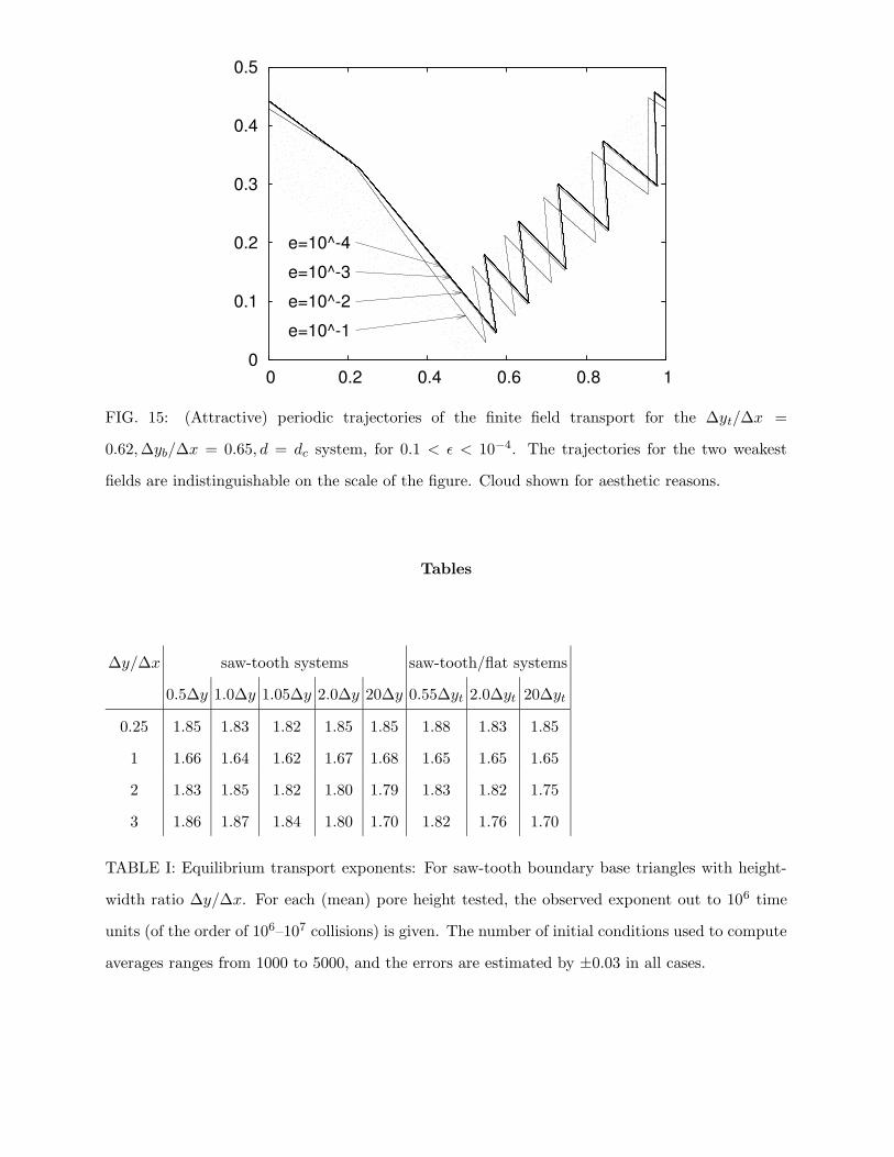
41

0

0.1

0.2

0.3

0.4

0.5

0 0.2 0.4 0.6 0.8 1

e=10^-1e=10^-2e=10^-3e=10^-4

FIG. 15: (Attractive) periodic trajectories of the finite field transport for the ∆yt/∆x =

0.62,∆yb/∆x = 0.65, d = dc system, for 0.1 < ε < 10−4. The trajectories for the two weakest

fields are indistinguishable on the scale of the figure. Cloud shown for aesthetic reasons.

Tables

∆y/∆x saw-tooth systems saw-tooth/flat systems

0.5∆y 1.0∆y 1.05∆y 2.0∆y 20∆y 0.55∆yt 2.0∆yt 20∆yt

0.25 1.85 1.83 1.82 1.85 1.85 1.88 1.83 1.85

1 1.66 1.64 1.62 1.67 1.68 1.65 1.65 1.65

2 1.83 1.85 1.82 1.80 1.79 1.83 1.82 1.75

3 1.86 1.87 1.84 1.80 1.70 1.82 1.76 1.70

TABLE I: Equilibrium transport exponents: For saw-tooth boundary base triangles with height-

width ratio ∆y/∆x. For each (mean) pore height tested, the observed exponent out to 106 time

units (of the order of 106–107 collisions) is given. The number of initial conditions used to compute

averages ranges from 1000 to 5000, and the errors are estimated by ±0.03 in all cases.

42

∆yt/∆x ∆yb/∆x saw-tooth systems

0.5∆y 1.0∆y 1.05∆y 2.0∆y 20∆y

0.62 0.63 1.00(2) 1.02(2) 0.97(3) 1.03(7) 0.72(3)

0.62 0.64 1.00(1) 1.2(1) 1.03(3) 1.19(7) 1.10(5)

0.62 0.65 0.99(2) 1.02(2) 1.02(3) 0.97(6) 1.13(5)

TABLE II: Equilibrium transport exponents: For unparallel saw-tooth boundary base triangles

with height-width ratio ∆y/∆x. For each (mean) pore height tested, the observed exponent out to

106 time units (of the order of 106–107 collisions) is given. The number of initial conditions used to

compute averages varies from 2000 up to 104. Numbers in brackets correspond to error estimates

from Marquardt-Levenberg least-squares fits.

field strength ε parallel system parallel system unparallel system unparallel system

(raw) (corrected) (raw) (corrected)

0.1 0.0935± 0.0001 0.0935± 0.0001 2.390± 0.003 2.390± 0.003

0.01 9.75± 0.2 0.205± 0.008 18.3± 0.2 0.24± 0.04

0.001 0.57± 0.04 0.57± 0.04 11± 1 0.19± 0.02

0.0001 0.28± 0.4 0.28± 0.4 1.2± 1 0.28± 0.14

equilibrium ∞ ∞ 0.386± 0.05 0.386± 0.05

TABLE III: Best estimates of the finite field diffusion coefficient D(ε; t) for 0.1 < ε < 10−4, t = 106

for the parallel ∆y/∆x = 2 system, and the unparallel ∆yt/∆x = 0.62,∆yb/∆x = 0.65, d = dc

system, showing the raw data and data corrected for periodic orbits. Also included, for comparison,

are the equilibrium results for the parallel case (exhibiting super-diffusive behaviour) and the

unparallel case.

∆yt/∆x ∆yb/∆x γ ∆yt/∆x ∆yb/∆x γ

1 1.01 0.71(4) 2 2.02 1.04(2)

1 1.001 0.35(6) 2 2.002 1.01(2)

1 1.0001 0.66(5) 2 2.0002 1.04(2)

1 1.00001 0.58(3) 2 2.00002 1.02(2)

1 1.000001 0.53(5) 2 2.000002 0.98(2)

1 1 1.66(3) 2 2 1.83(3)

43

TABLE IV: Transport law exponent γ, as identified by (20), observed for various choices of ∆yt/∆x

and ∆yb/∆x. There appears to be no trend toward super-diffusive transport, arbitrarily close to

(but away from) the parallel case. Numbers in brackets indicate errors in the last figure.