THERMAL MECHANICAL ANALYSIS OF APPLICATIONS WITH …

THERMAL MECHANICAL ANALYSIS

OF APPLICATIONS WITH

INTERNAL HEAT GENERATION

_______________________________________

A Dissertation

presented to

the Faculty of the Graduate School

at the University of Missouri-Columbia

_______________________________________________________

In Partial Fulfillment

of the Requirements for the Degree

Doctor of Philosophy

_____________________________________________________

by

SRISHARAN GARG GOVINDARAJAN

Dr. Gary Solbrekken, Dissertation Supervisor

DECEMBER 2014

The undersigned, appointed by the dean of the Graduate School, have examined the

dissertation entitled

THERMAL MECHANICAL ANALYSIS

OF APPLICATIONS WITH

INTERNAL HEAT GENERATION

presented by Srisharan Garg Govindarajan,

a candidate for the degree of doctor of philosophy,

and hereby certify that, in their opinion, it is worthy of acceptance.

Professor Gary Solbrekken

Professor Chung Lung Chen

Professor Robert Winholtz

Professor Hani Salim

ii

ACKNOWLEDGEMENTS

I am grateful to my supervisor Dr. Gary Solbrekken for having guided me through

this dissertation with his patience and knowledge, while giving me the independence to

work in my own way. My family has been a great source of support through all these

years and I would like to thank them for believing in me and making this possible. I am

also fortunate to have made some great friends during my time as a graduate student and

they have certainly helped me tide over difficult periods with all their encouragement.

Interacting and working with accomplished researchers has greatly benefitted me

and I would like to thank Dr. George Vandegrift at the Argonne National Laboratory,

Charlie Allen from the Missouri University Research Reactor, Dr. Sherif El-Gizawy at

the University of Missouri, Chris Bryan, Dr. James Freels, Dr. Prashanth Jain, Dr. David

Chandler, Dr. Paul Williams, Larry Ott, Randy Hobbs, Cliff Hayman, Fred Griffin, and

Christopher Hurt at the Oak Ridge National Laboratory.

Finally, I would like to thank my colleagues, Dr. Kyler Turner, John Kennedy,

Philip Makarewicz, Casey Jesse, Brian Graybill, Annemarie Hoyer, and Alex Moreland,

for offering their perspectives on various issues during the course of this dissertation.

iii

TABLE OF CONTENTS

ACKNOWLEDGEMENTS ................................................................................................ ii

LIST OF FIGURES .......................................................................................................... vii

LIST OF TABLES ........................................................................................................... xiv

NOMENCLATURE ..........................................................................................................xv

ABSTRACT ..................................................................................................................... xvi

Chapter

1. INTRODUCTION ...................................................................................................1

1.1 Molybdenum-99 and Technetium-99m .......................................................2

1.2 Production Methods and Target Development ............................................4

1.3 Thermal Contact Resistance ........................................................................8

1.4 Control Blades ...........................................................................................10

1.5 Objective of Work......................................................................................12

2. LITERATURE REVIEW ......................................................................................14

2.1 Target Design and Irradiations...................................................................14

2.2 Thermal Contact Resistance ......................................................................17

2.3 Thermal Stresses in Cylinders ...................................................................20

2.4 Fission Gas Release and Uranium Swelling ..............................................22

3. ANNULAR TARGET THERMAL- MECHANICAL SAFETY ANALYSIS .....24

3.1 Target Design .............................................................................................24

3.2 Plate Target ................................................................................................24

3.3 Annular Target ...........................................................................................26

4. MODELING WITHOUT RESIDUAL STRESSES ..............................................31

iv

4.1 Non-Uniform Heating Numerical Model...................................................31

4.2 Uniform Heating Numerical Model ...........................................................41

4.3 Uniform Heating Analytical Model- Dimensional Form...........................43

4.4 Uniform Heating Analytical Model- Sensitivity Studies ...........................58

5. MODELING WITHOUT RESIDUAL STRESSES - RESULTS .........................61

5.1 Uniform Heating- Analytical and Numerical ............................................61

5.2 Non-Uniform Heating ................................................................................68

5.3 Uniform and Non-Uniform Heating Comparison ......................................76

5.4 Uniform Heating Sensitivity Studies .........................................................81

6. DIMENSIONLESS ANALYTICAL MODEL - UNIFORM HEATING .............94

6.1 Dimensionless Thermal-Mechanical Expressions .....................................94

6.2 Dimensionless Model Results ..................................................................100

7. MODELING WITH RESIDUAL STRESSES ....................................................104

7.1 Hydroforming Assembly Description ......................................................105

7.2 Draw-Plug Assembly Description ...........................................................107

8. HYDROFORMING ASSEMBLY AND IRRADIATION ANALYSIS .............108

8.1 Material Model.........................................................................................108

8.2 Numerical Finite Element Model.............................................................109

8.3 Hydroforming Analysis Results ...............................................................113

9. DRAW-PLUG ASSEMBLY AND IRRADIATION ANALYSIS......................119

9.1 Material Model.........................................................................................119


9.3 Draw-Plug Analysis Results ....................................................................124

v

10. INTERFACIAL PHENOMENA AND URANIUM SWELLING ......................130

10.1 Fission Gas Release and Uranium Swelling Model .................................130

10.2 Interfacial Conductance Model ................................................................136

10.3 Additional Effects ....................................................................................141

10.4 Numerical Model .....................................................................................142

10.5 Results ......................................................................................................143

11. REACTOR SPECIFIC ANNULAR TARGET ANALYSIS ...............................149

11.1 Reactor Description .................................................................................149

11.2 Target Geometry ......................................................................................151

11.3 Calculation of Input .................................................................................153

11.4 Finite Element Model Development ........................................................155

11.5 Results ......................................................................................................161

11.6 Technical Adequacy and Independent Review Comments .....................167

12. BORAL CONTROL BLADE SAFETY ANALYSIS .........................................168

12.1 Control Blade Geometry and Model Development .................................168

12.2 Heating Profile Development ..................................................................171


12.4 Results ......................................................................................................181

13. CONCLUSIONS AND RECOMMENDATIONS ..............................................183

APPENDIX ......................................................................................................................187

1. Mathematica Code to Determine Heat Flux ........................................................187

2. Mathematica Code to Determine Outer Tube Parameters ...................................189

3. Mathematica code to Determine Inner Tube Parameters .....................................190

vi

4. Mathematica Code to Determine Contact Pressure .............................................192

5. Mathematica Code to Calculate Fission Gas Pressure .........................................194

6. Mathematica Code to Develop a Thermal Conductance Model for

Al 6061-T6 and Al 6061-T6 Interface .................................................................197


Al 6061-T6 and Nickel Interface .........................................................................200


Uranium and Nickel interface ..............................................................................203


Al 6061-T4 and Al 6061-T4 interface .................................................................206


Al 6061-T4 and Pure Al interface ........................................................................209

11. Abaqus Input File for the Planar Model with Non-Uniform Heating ..................212

12. Abaqus Input File for the Hydroforming and Irradiation Model .........................215

13. Abaqus Input File for the Draw-Plug Based Irradiation Model ..........................227

14. Abaqus Input File for the Control Blade Analysis...............................................246

REFERENCES ................................................................................................................249

VITA ................................................................................................................................261

vii

LIST OF FIGURES

Figure Page

1. (a) Australian Nuclear Science and Technology Organization's (ANSTO)

technetium generator external view. (b) General internal structure of a

technetium generator.. ..............................................................................................3

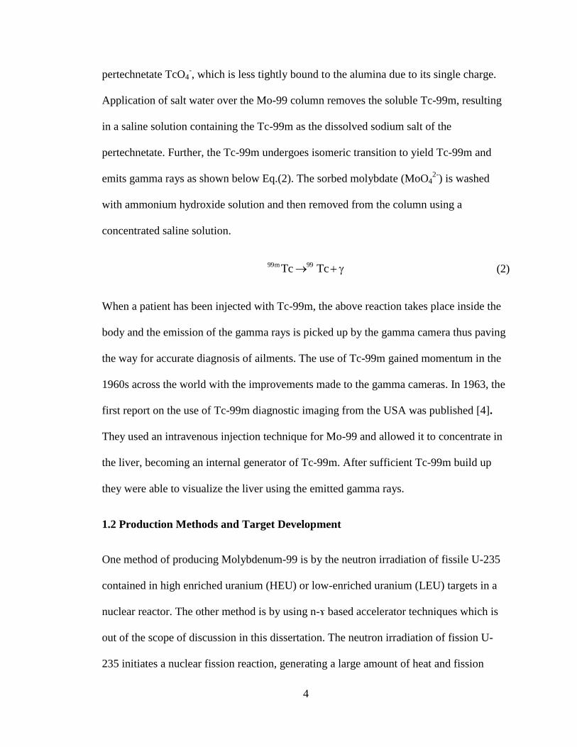
2. Traditional powder dispersion method using HEU. ................................................5

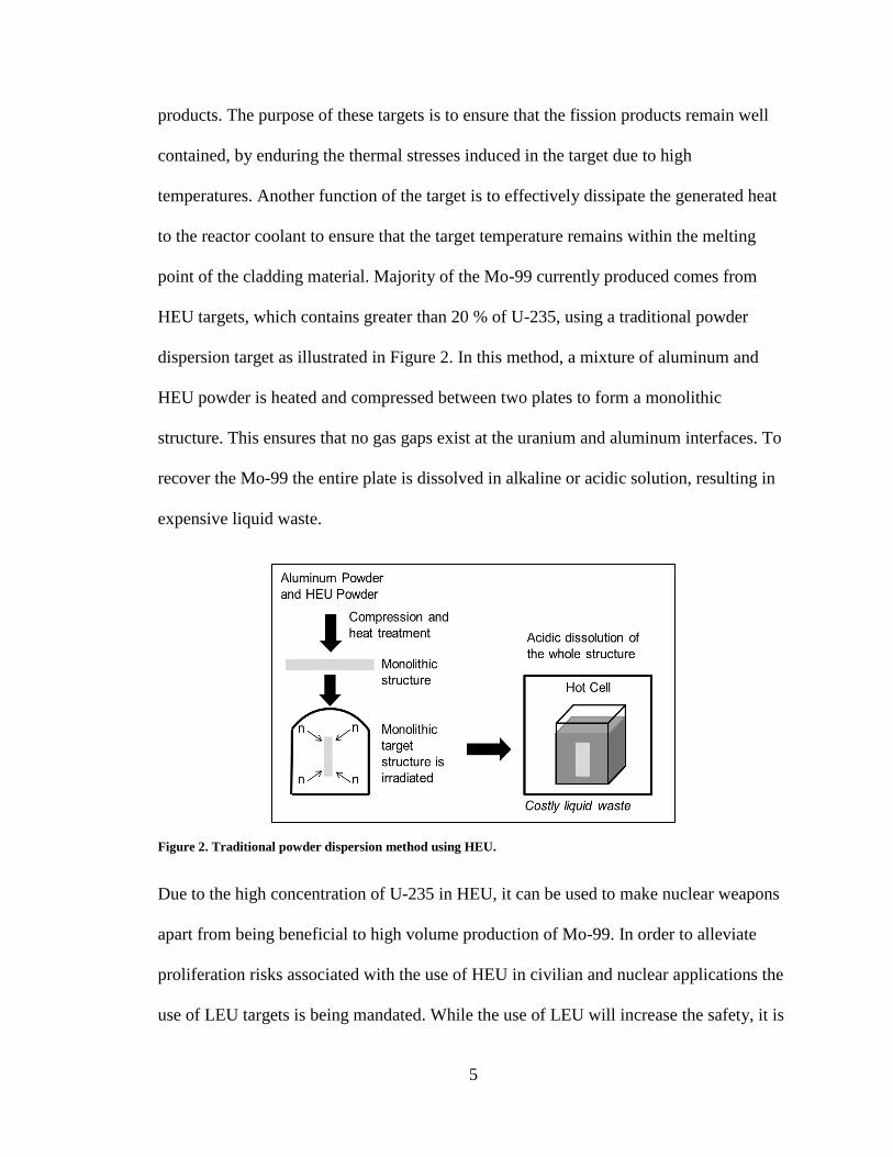
3. Mo-99 activity vs. uranium density for HEU and LEU dispersion. ........................6

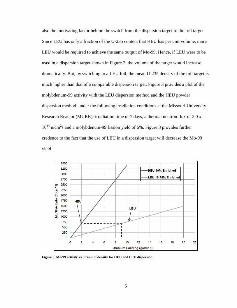
4. Proposed LEU metal foil based approach for Mo-99 production. ...........................7

5. Hot cells at (a) Comision Nactional de Energia Atomica (CNEA) in Argentina,

and (b) Missouri University Research Reactor (MURR).. ......................................8

6. Surface irregularities offering resistance to heat flow through a compound

cylinder assembly.....................................................................................................9

7. MURR core showing the reflector, control blade and pressure vessel.. ................11

8. Flat plate target with welded edges. .......................................................................25

9. Curved plate type target with welded edges. .........................................................25

10. A simple diagram of the annular target illustrating the position of the foil

longitudinally and the location of the circumferential gap. ...................................26

11. A prototype annular target with welded edges. .....................................................27

12. Interfacial contact bond formed by solid contact spots and interstitial gaps. ........27

13. Sketch depicting the resistances across the interfacial thickness...........................28

14. Annular target design using Al 3003-H14 as the cladding.. ..................................30

15. Pictorial representation of the modeling strategy for the analysis of the

annular target without initial residual stresses. ......................................................32

16. Numerical model assembly showing: (a) The inner tube alone with the recess

and (b) The inner tube after the addition of the outer tube. ...................................32

17. Pictorial representation of the position of the annular target in the vertical

experimental facility relative to the reactor core. ..................................................33

18. Numerical setup of the 2D plane strain model of the annular target modeled

without the nickel recoil barrier. ............................................................................34

19. Annular target assembly procedure in Abaqus FEA..............................................35

viii

20. Mechanical boundary condition applied to the annular target assembly. ..............37

21. Representation of the coolant flow internally and through the annulus. ...............38

22. Finite element mesh used to simulate the non-uniform heating model. ................41

23. Setup of the uniform heating 2D plane strain model of the annular target. ...........42

24. Mechanical boundary conditions used in the uniform heating model. ..................43

25. Symbolic dimensions and thermal resistance network of the uniform heating

annular target case..................................................................................................44

26. Representation of the simplified solution approach for stresses and

displacement. .........................................................................................................48

27. Circumferential temperature distribution on the inner and outer cladding for

uniform heating with q'''=1.6 x 1010

W/m3. ..........................................................61

28. Assembly temperature distribution contour for uniform heating with

q'''=1.6x1010

W/m3. ................................................................................................62

29. Radial temperature distribution in the cladding for q'''=1.6 x 1010

W/m3

and uniform heating. ..............................................................................................62

30. Radial stress distribution in the cladding at θ=270ᵒfor uniform heating with

q"'=1.6x1010

W/m3. ................................................................................................63

31. Radial stress distribution contour of the assembly for uniform heating with

q'''=1.6x1010

W/m3. ................................................................................................64

32. Hoop stress distribution in the cladding at θ=270ᵒ for uniform heating at

q'''=1.6x1010

W/m3. ................................................................................................64

33. Hoop stress distribution contour of the assembly for uniform heating

with q'''=1.6x1010

W/m3. ........................................................................................65

34. Separation between the foil and the outer tube for uniform heating with

q'''=1.6x1010

W/m3. ................................................................................................66

35. Interfacial separation between the foil and the outer tube cladding for

uniform heating with q'''=1.6x1010

W/m3. .............................................................66

36. Circumferential contact pressure distribution in the inner tube for uniform

heating with q'''=1.6x1010

W/m3. ...........................................................................67

37. Assembly temperature distribution contour for non-uniform heating. ..................68

38. Radial stress and temperature distribution for non-uniform heating. ....................69

39. Radial displacement contour illustrating the interfacial separation between

the foil and the cladding for non-uniform heating. ................................................70

ix

40. Hoop stress and separation along the circumference of the outer tube inner

surface for non-uniform heating. ...........................................................................70

41. Assembly hoop stress contour for non-uniform heating. .......................................70

42. Temperature and hoop stresses in the outer tube for non-uniform heating. ..........72

43. Interfacial separation and contact pressure variation in the inner surface

of the outer tube for non-uniform heating..............................................................72

44. Temperature and hoop stresses in the inner tube for non-uniform heating ...........73

45. Contact pressure in the inner tube outer surface for non-uniform heating. ...........74

46. Deformed and un-deformed radial distribution contours of the inner tube for

non-uniform heating...............................................................................................75

47. Deformed and un-deformed radial distribution contours of the outer tube for


48. Deformed and un-deformed radial displacement contours of the LEU foil for


49. Final deformed shape of the annular target post irradiation for non-uniform

heating. ...................................................................................................................75

50. Assembly temperature distribution comparison for uniform and non-uniform

heating. ...................................................................................................................77

51. Circumferential temperature distribution on the outer surface of the inner

tube: comparison between uniform and non-uniform heating. ..............................77

52. Circumferential temperature distribution on the inner surface of the

outer tube: comparison between uniform and non-uniform heating. .....................78

53. Assembly radial stress distribution comparison for uniform and non-uniform

heating. ...................................................................................................................78

54. Comparison of contact pressure on the outer surface of the inner tube for

uniform and non-uniform heating. .........................................................................79

55. Comparison of hoop stresses on the outer surface of the inner tube for


56. Comparison of hoop stresses on the inner surface of the outer tube for


57. Comparison of the magnitude of separation at the interface of the foil and

the outer tube for uniform and non-uniform heating conditions............................80

x

58. Radial temperature distributionin the inner and outer tubes for varying

LEU heat generation rates with Twall =373 K for uniform heating. ......................82

59. Radial stress distribution in the inner and outer tubes for varying LEU heat

generation rates with Twall =373 K for uniform heating. .......................................82

60. Hoop stress distribution in the inner and outer tubes for varying LEU heat

generation rates with Twall =373 K for uniform heating. .....................................83

61. Temperature variation on the surfaces of the tubes with varying heat transfer

coefficient ratios with Twall = 373 K for uniform heating. .....................................84

62. (a) Radial stress distribution and (b) contact pressure on the outer surface of

the inner tube for varying heat transfer coefficient ratios with Twall=373 K for

uniform heating. .....................................................................................................85

63. Hoop stress distribution in the inner and outer tubes for varying heat transfer

coefficient ratios with Twall = 373 K for uniform heating. .....................................85

64. Separation at the interface of the outer tube and LEU foil for varying

heat transfer coefficient ratios with Twall= 373 K for uniform heating. .................86

65. Hoop stress in the inner tube for varying heat transfer coefficient ratios with

Twall =373 K for uniform heating. ..........................................................................87

66. Cladding temperature distribution for varying LEU heat generation rates

with the heat transfer coefficient ratio H=1, with no restrictions on wall

temperature and for uniform heating. ....................................................................88

67. Radial stress distribution in the cladding for varying LEU heat generation

rates with the heat transfer coefficient ratio H=1, with no restrictions on wall

temperatures and for uniform heating. ...................................................................88

68. Hoop stress distribution in the cladding for varying LEU heat generation rates

with the heat transfer coefficient ratio H=1, with no restrictions on wall

temperature and for uniform heating. ....................................................................89

69. Temperature distribution in the cladding with varying heat transfer coefficient

ratios for uniform heating with no restrictions on wall temperature. ....................90

70. Radial stress and contact pressure distribution in the inner tube outer surface

with varying heat transfer coefficient ratios for uniform heating with no

restrictions on wall temperature. ............................................................................91

71. Hoop stress distribution in the cladding with varying heat transfer coefficient

ratios for uniform heating with no restrictions on wall temperature. ....................92

72. Separation at the interface of the foil and the outer tube with varying heat

transfer coefficient ratios for uniform heating and no restrictions on wall

temperature. ...........................................................................................................92

xi

73. Variation of hoop stress in the inner tube at H=1 for different tube thickness

ratios and LEU heat generation rates. ....................................................................93

74. Hoop stress in the inner tube at q'''=1.6 E10 W/m3 at various tube thickness

and heattransfer coefficient ratios. .........................................................................93

75. Dimensionless radial temperature distribution in the annular target. ..................100

76. Dimensionless radial stress distribution in the annular target. ............................101

77. Dimensionless hoop stress distribution in the inner tube and the outer tube. ......102

78. Dimensionless radial displacement in the inner tube and the LEU foil ...............102

79. Dimensionless radial displacement in the outer tube. ..........................................103

80. The draw-plug and the hydroforming assembly techniques. ...............................104

81. Drawing of the geometry in the first analysis step of the assembly

simulation model. .................................................................................................106

82. (a) Hydroforming test rig with the annular target in place and (b) assembled

hydroforming test rig. ..........................................................................................106

83. Pre-assembly state of the annular target. .............................................................107

84. Draw-plug assembly device. ................................................................................107

85. True stress and plastic strain curves for Al 6061-T6 and uranium. .....................109

86. Finite element mesh used in the assembly and irradiation modeling. .................110

87. Loading and mechanical boundary conditions for the assembly

hydroforming simulation in the first analysis step. ..............................................111

88. Loading and boundary conditions for the irradiation model ...............................112

89. Numerical displacement contour and microscopic images of the annular

target after the assembly process. ........................................................................113

90. Equivalent plastic strain across the radius of the annular target at θ=270ᵒ. .........114

91. Separation at the interface of the foil and the outer tube after the various

modeling steps. ....................................................................................................115

92. Radial temperature distribution across the inner and the outer cladding. ............116

93. Hoop stress distribution in the inner tube through various modeling steps .........117

94. Hoop stress distribution in the outer tube through various modeling steps .........118

95. True stress and plastic strain curve for nickel used in the numerical model. ......120

xii

96. Pre-assembly target tubes and the plug dimensions. ...........................................121

97. The model change command in Abaqus to remove the plug. ..............................122

98. The three-step axisymmetric modeling procedure with boundary and

loading conditions. ...............................................................................................123

99. Finite element mesh used in the draw-plug based analysis. ................................124

100. Sectioning locations along the assembled target length. .....................................125

101. Post-assembly views of the sectioned images against the numerical model. ......126

102. Longitudinal separation at the outer tube interface. .............................................126

103. Equivalent plastic strain across the thickness at half the target length. ...............127

104. Hoop stress distribution across the cladding thickness. .......................................128

105. Longitudinal temperature distribution for Target-1 and Target-2. ......................129

106. Irradiation stress state of Target-1 and Target-2. .................................................129

107. The dependence of swelling on temperature for high purity uranium .................136

108. Mechanical and thermal loading during the irradiation step. ..............................142

109. Volumetric swelling strain rate definition location. ............................................143

110. Von Mises stresses in the cladding for case-1 compared against Target-2

values from Figure 107. .......................................................................................145

111. Thermal contact conductance as a function of pressure for various interfacial

combinations. .......................................................................................................145

112. Radial temperature distribution in the annular target for case-1 ..........................146

113. Variation of maximum temperature with the heat generation rate for case-4. ....148

114. Variation of von Mises stresses with the heat generation rate for case-5. ...........148

115. Aerial view of the HFIR facility. .........................................................................150

116. The HFIR core illustrating the location of the experimental facilities ................150

117. Pre-assembly annular target dimensions for HFIR irradiation. ...........................151

118. Dimensions of the draw-plug used to assemble the annular target with the

6061-T4 Al cladding. ...........................................................................................152

119. Material models for Al 6061-T4 and uranium. ....................................................153

120. Draw-plug assembly model setup for the HFIR annular target. ..........................157

xiii

121. Finite element mesh of the assembly model for the HFIR annular target. ..........158

122. Irradiation model setup for the HFIR annular target. ..........................................159

123. Finite element mesh of the irradiation model for the HFIR annular target. ........160

124. Von Mises stress distribution in the cladding for the HFIR annular target. ........164

125. Radial temperature distribution in the HFIR annular target ................................164

126. Longitudinal temperature distribution in the inner tube for the HFIR target. .....165

127. Longitudinal temperature distribution in the outer tube for the HFIR target. .....166

128. Dimensions of the BORAL control blade. ...........................................................169

129. A cross- sectional view of the MCNP MURR core model ..................................170

130. Linearized exponential decay function for a given thickness and azimuthal

location for alpha heating.....................................................................................173

131. 'A' and 'B' coefficient variations with thickness in BORAL core for alpha

heating at left edge location. ................................................................................173

132. 'A' and 'B' coefficient variation with thickness in the BORAL core for gamma

heating at the left edge location. ..........................................................................173

133. Alpha heat generation data and fit through the BORAL core at the left edge. ....175

134. Alpha heat generation data and fit at the fuel-side BORAL face. .......................175

135. Components of the assembled control blade along with the mechanical

boundary conditions. ............................................................................................180

136. Finite element mesh of the (a) BORAL meat and (b) aluminum cladding

used in the Abaqus model. ...................................................................................180

137. (a) Temperature distribution contour of the control blade and (b) variation of

temperature along the cladding centerline. ..........................................................182

138. (a) Radial deflection contour and (b) deflection variation on the sides of the

control blade.........................................................................................................182

139. Deflection variation along the length of the control blade with varying

thermal conductivity of the BORAL. ...................................................................182

xiv

LIST OF TABLES

Table Page

1. Material properties of the foil and the cladding used in the analysis. ....................34

2. Mesh configuration for the non-uniform heating numerical model without

residual stresses. .....................................................................................................40

3. LEU heat generation rates used in the sensitivity studies. .....................................58

4. Heat transfer coefficient parametric study for wall temperatures maintained

at 373 K. .................................................................................................................59

5. Heat transfer coefficient study with no restriction on wall temperature. ...............60

6. Tube thickness variation study...............................................................................60

7. Percent difference comparison between the analytical and numerical models

for the inner and the outer tubes. ...........................................................................67

8. Uniform and non-uniform heating comparison summary. ....................................81

9. Material properties used in the draw plug model.................................................120

10. Post assembly target measurements: Measured vs. model results. ......................125

11. Properties and of quantity of gases used in the calculations. ...............................131

12. Material and surface properties of the metals. .....................................................138

13. Thermophysical properties of the gases in the gap conductance calculations. ....140

14. Maximum von Mises stress variation with the addition of constraints. ..............144

15. Maximum cladding temperature variation with the addition of constraints. .......146

16. Material properties used in the calculations.........................................................152

17. Properties of the fission gases used in the reactor specific calculations. .............154

18. Assembled dimensions of the annular target: measurement vs. model results. ...162

19. Maximum residual stresses in the inner and outer tubes .....................................162

20. Annular target temperature results for the safety basis analysis. .........................163

21. Alpha volumetric heat generation data and fit comparison at the left edge.........176

22. Material properties of the BORAL and the aluminum cladding used in the

analysis. ................................................................................................................180

xv

NOMENCLATURE

Cp heat capacity n number of moles Subscripts

B virial coefficient q power F foil

D diameter q" heat flux IF interface

E elastic modulus q'''

volumetric heat

generation IT inner tube

G shear modulus r radius OT outer tube

H microhardness u displacement cond conduction

L length x mass fraction conv convection

M molecular mass y mole fraction eff effective

Nu Nusselt number Greek gen generation

P pressure α thermal expansion

coefficient fD fully developed

Pr Prandtl number β accommodation

coefficient in inner surface

Q dimensionless heat

generation Δ quantitative change out outer surface

R dimensionless radius δ gap thickness max maximum

R' thermal resistance ε strain Abbreviation

Re Reynolds number γ ratio of specific heat ANL Argonne national lab

T temperature κ bulk modulus DOE Department of energy

U total interference λ mean free path FEA finite element analysis

V flow velocity ϕ asperity slope HEU high enriched uranium

Z compressibility factor Ψ plasticity index HFIR high flux isotope reactor

f fissions ρ density LEU low enriched uranium

g temperature jump

distance µ dynamic viscosity MURR

Missouri university

research reactor

h heat transfer

coefficient υ Poisson’s ratio ORNL

Oak ridge national

laboratory

h' thermal conductance σ stress (or) roughness PVD physical vapor

deposition

k thermal conductivity θ dimensionless

temperature

xvi

ABSTRACT

The radioactive tracer Technetium-99m is widely used in medical imaging and is derived

from its parent isotope Molybedenum-99 (Mo-99) by radioactive decay. The majority of

Molybdenum-99 (Mo-99) produced internationally is extracted from high enriched

uranium (HEU) dispersion targets that have been irradiated. To alleviate proliferation

risks associated with HEU-based targets, the use of non-HEU sources is being mandated.

However, the conversion of HEU to LEU based dispersion targets affects the Mo-99

available for chemical extraction. A possible approach to increase the uranium density, to

recover the loss in Mo-99 production-per-target, is to use an LEU metal foil placed

within an aluminum cladding to form a composite structure. The target is expected to

contain the fission products and to dissipate the generated heat to the reactor coolant. In

the event of interfacial separation, an increase in the thermal resistance could lead to an

unacceptable rise in the LEU temperature and stresses in the target. The target can be

deemed structurally safe as long as the thermally induced stresses are within the yield

strength of the cladding and welds.

As with the thermal and structural safety of the annular target, the thermally induced

deflection of the BORAL®-based control blades, used by the University of Missouri

Research Reactor (MURR®), during reactor operation has been analyzed. The boron,

which is the neutron absorber in BORAL, and aluminum mixture (BORAL meat) and the

aluminum cladding are bonded together through powder metallurgy to establish an

adherent bonded plate. As the BORAL absorbs both neutron particles and gamma rays,

there is volumetric heat generation and a corresponding rise in temperature. Since the

BORAL meat and aluminum cladding materials have different thermal expansion

xvii

coefficients, the blade may have a tendency to deform as the blade temperature changes

and the materials expand at different rates. In addition to the composite nature of the

control blade, spatial variations in temperature within the control blade occur from the

non-uniform heat generation within the BORAL as a result of the non-uniform thermal

neutron flux along the longitudinal direction when the control blade is partially

withdrawn. There is also variation in the heating profile through the thickness and about

the circumferential width of the control blade. Mathematical curve-fits are generated for

the non-uniform volumetric heat generation profile caused by the thermal neutron

absorption and the functions are applied as heating conditions within a finite element

model of the control blade built using the commercial finite element code Abaqus FEA.

The finite element model is solved as a fully coupled thermal mechanical problem as in

the case of the annular target. The resulting deflection is compared with the channel gap

to determine if there is a significant risk of the control blade binding during reactor

operation.

Hence, this dissertation will consist of two sections. The first section will seek to present

the thermal and structural safety analyses of the annular targets for the production of

molybdenum-99. Since there hasn’t been any detailed, documented, study on these

annular targets in the past, the work complied in this dissertation will help to understand

the thermal-mechanical behavior and failure margins of the target during in-vessel

irradiation. As the work presented in this dissertation provides a general performance

analysis envelope for the annular target, the tools developed in the process can also be

used as useful references for future analyses that are specific to any reactor. The

numerical analysis approach adopted and the analytical models developed, can also be

xviii

applied to other applications, outside the Mo-99 project domain, where internal heat

generation exists such as in electronic components and nuclear reactor control blades.

The second section will focus on estimating the thermally induced deflection and hence

establish operational safety of the BORAL control blades used at the Missouri University

Research Reactor (MURR) to support their relicensing efforts with the Nuclear

Regulatory Commission (NRC). The common theme in both these sections is the nuclear

heat source, high heat flux, non-uniform heating, composite structures and differential

thermal expansion. The goal is to establish the target and component operational safety,

and also provide documented analysis that can be referred to in the future.

1

Chapter 1: Introduction

In 1934, Marie and Pierre Curie reported the first artificial production of radioactive

material, after discovering radioactivity in aluminum foil that was irradiated with a

polonium preparation. The discoveries by Wilhelm Konrad Roentgen (X-ray), Marie

Curie (radioactive thorium and coining the term ‘radioactivity’) and Henri Becquerel

(radioactive uranium salts), formed the basis for their work. An article [1] published in

the Journal of the American Medical Association in 1946 described the successful

application of Iodine-131, a radioisotope, to treat a patient with thyroid cancer

metastases. This provided the much needed boost to the field of nuclear medicine and led

to extensive research and development of non-invasive medical procedures to provide

diagnostic treatment to patients. Positron emission tomography (PET), magnetic

resonance imaging (MRI), computed X-ray tomography (CT), single-photon emission

computed tomography (SPECT), and X-rays, are some of the non-invasive medical

techniques. These procedures involving nuclear medicine employ the use of radioactive

tracers which emit gamma rays from within the body. The tracers are short lived isotopes

linked to chemical compounds which permit specific physiological processes to be

examined. For example, PET uses radio nuclides that are isotopes with short half-lives

such as fluorine-18 (~110 minutes), carbon-11 (~20 minutes), nitrogen-13 (~ 10 minutes)

and oxygen-15 (~2 minutes). These radio nuclides are either injected into the patient’s

bloodstream or given orally so that they interact with the compounds normally used by

the body such as glucose, water, or ammonia. The positron emitting radionuclide

accumulates in the area of concern and emits a positron that combines with an electron to

emit gamma rays in opposite directions which are picked up by PET gamma cameras.

2

Apart from being helpful in cardiac and brain imaging, the PET has been found to be

very accurate in detecting and evaluating cancers. Despite advances in other imaging

methods such as CT and MRI, the ability to image the metabolic abnormalities associated

with a disease has made PET one of the most significant diagnostic tools. Amongst all the

radio nuclides used in various medical procedures, Technetium-99m is the most

commonly used diagnostic radioactive tracer element and more information about the

same can be found in the following section.

1.1 Molybdenum-99 and Technetium-99m

Molybdenum, a transition metal found in group 6 in the periodic table, was discovered in

1778 by Carl Wilhelm Scheele. There are approximately 35 recognized isotopes of

molybdenum, with atomic mass numbers ranging from 83 to 117. The isotopes with

atomic masses 92, 94, 95, 96, 97, 98 and 100 occurs naturally while the isotope with

atomic mass of 100 is considered to be unstable [2]. Molybdenum-99 (Mo-99) is obtained

as a fission product after neutron irradiation of uranium-235 (U-235). Technetium-99m

(Tc-99m) is the daughter isotope of Mo-99, was discovered in 1937 by Carlo Perrier (an

Italian mineralogist) and Emilio Gino Segre (a Nobel laureate in physics), to fill space

number 43 in the periodic table. In 1940, Emilio Segre and Chien-Wu performed

experiments to analyze the fission products of U-235 which contained Mo-99 [3].Their

analysis results helped them conclude that the element 43 had a 6 hour half-life. The short

half-life of Tc-99m (6 hours) restricts it from being transported. Due to this, the Mo-99

(half-life of 66 hours) is directly shipped to hospitals and radio-pharmacies in radiation

shielded containers known as technetium generators (Figure 1). The Mo-99, with its 66

hour half-life, decays to Tc-99m. As shown in Figure 1[9], the Tc-99m can be obtained

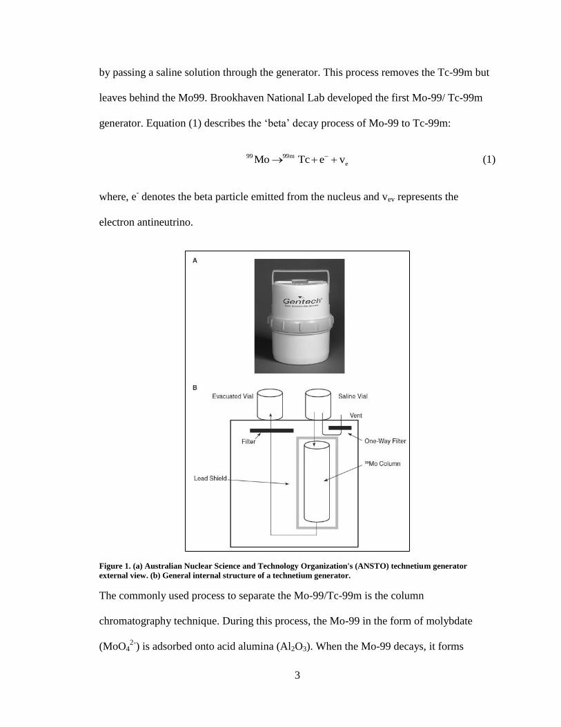
3

by passing a saline solution through the generator. This process removes the Tc-99m but

leaves behind the Mo99. Brookhaven National Lab developed the first Mo-99/ Tc-99m

generator. Equation (1) describes the ‘beta’ decay process of Mo-99 to Tc-99m:

99 99m

eMo Tc e v (1)

where, e- denotes the beta particle emitted from the nucleus and vev represents the

electron antineutrino.

Figure 1. (a) Australian Nuclear Science and Technology Organization's (ANSTO) technetium generator

external view. (b) General internal structure of a technetium generator.

The commonly used process to separate the Mo-99/Tc-99m is the column

chromatography technique. During this process, the Mo-99 in the form of molybdate

(MoO42-

) is adsorbed onto acid alumina (Al2O3). When the Mo-99 decays, it forms

4

pertechnetate TcO4-, which is less tightly bound to the alumina due to its single charge.

Application of salt water over the Mo-99 column removes the soluble Tc-99m, resulting

in a saline solution containing the Tc-99m as the dissolved sodium salt of the

pertechnetate. Further, the Tc-99m undergoes isomeric transition to yield Tc-99m and

emits gamma rays as shown below Eq.(2). The sorbed molybdate (MoO42-

) is washed

with ammonium hydroxide solution and then removed from the column using a

concentrated saline solution.

99m 99Tc Tc (2)

When a patient has been injected with Tc-99m, the above reaction takes place inside the

body and the emission of the gamma rays is picked up by the gamma camera thus paving

the way for accurate diagnosis of ailments. The use of Tc-99m gained momentum in the

1960s across the world with the improvements made to the gamma cameras. In 1963, the

first report on the use of Tc-99m diagnostic imaging from the USA was published [4].

They used an intravenous injection technique for Mo-99 and allowed it to concentrate in

the liver, becoming an internal generator of Tc-99m. After sufficient Tc-99m build up

they were able to visualize the liver using the emitted gamma rays.

1.2 Production Methods and Target Development

One method of producing Molybdenum-99 is by the neutron irradiation of fissile U-235

contained in high enriched uranium (HEU) or low-enriched uranium (LEU) targets in a

nuclear reactor. The other method is by using n-ɤ based accelerator techniques which is

out of the scope of discussion in this dissertation. The neutron irradiation of fission U-

235 initiates a nuclear fission reaction, generating a large amount of heat and fission

5

products. The purpose of these targets is to ensure that the fission products remain well

contained, by enduring the thermal stresses induced in the target due to high

temperatures. Another function of the target is to effectively dissipate the generated heat

to the reactor coolant to ensure that the target temperature remains within the melting

point of the cladding material. Majority of the Mo-99 currently produced comes from

HEU targets, which contains greater than 20 % of U-235, using a traditional powder

dispersion target as illustrated in Figure 2. In this method, a mixture of aluminum and

HEU powder is heated and compressed between two plates to form a monolithic

structure. This ensures that no gas gaps exist at the uranium and aluminum interfaces. To

recover the Mo-99 the entire plate is dissolved in alkaline or acidic solution, resulting in

expensive liquid waste.

Figure 2. Traditional powder dispersion method using HEU.

Due to the high concentration of U-235 in HEU, it can be used to make nuclear weapons

apart from being beneficial to high volume production of Mo-99. In order to alleviate

proliferation risks associated with the use of HEU in civilian and nuclear applications the

use of LEU targets is being mandated. While the use of LEU will increase the safety, it is

6

also the motivating factor behind the switch from the dispersion target to the foil target.

Since LEU has only a fraction of the U-235 content that HEU has per unit volume, more

LEU would be required to achieve the same output of Mo-99. Hence, if LEU were to be

used in a dispersion target shown in Figure 2, the volume of the target would increase

dramatically. But, by switching to a LEU foil, the mean U-235 density of the foil target is

much higher than that of a comparable dispersion target. Figure 3 provides a plot of the

molybdenum-99 activity with the LEU dispersion method and the HEU powder

dispersion method, under the following irradiation conditions at the Missouri University

Research Reactor (MURR): irradiation time of 7 days, a thermal neutron flux of 2.0 x

1014

n/cm2s and a molybdenum-99 fission yield of 6%. Figure 3 provides further

credence to the fact that the use of LEU in a dispersion target will decrease the Mo-99

yield.

Figure 3. Mo-99 activity vs. uranium density for HEU and LEU dispersion.

7

The alternative to HEU dispersion targets is to use LEU foil based targets, where the

LEU foil is wrapped in a nickel foil and sandwiched between two concentric aluminum

tubes to form a composite structure [6]. The role of the nickel foil is to act as a recoil

barrier [7] and prevent any bonding between the aluminum cladding and the LEU foil

during irradiation. After irradiation the aluminum cladding is cut open to retrieve the

LEU foil alone, which is then dissolved to retrieve the Mo-99. A pictorial representation

of this process is illustrated in Figure 4 with the annular target and the flat plate target [8].

Figure 4. Proposed LEU metal foil based approach for Mo-99 production.

Upon removal of the targets from the reactor after irradiation; they are cooled for about a

day before being transported to the processing facilities in radiation shielded containers.

The cooling of the targets is a safety measure to reduce the overall irradiation doses in the

target processing system, to prevent the target from being damaged due to the high

temperatures, and to provide time for short lived fission gases to decay. The chemical

processing of the targets takes place inside ‘hot cells’. Post-irradiation, approximately 1

% of the Mo-99 produced in the target is lost to radioactive decay every hour. Hence it is

important to quickly carry out the processing in the hot cell to recover the Mo-99. The

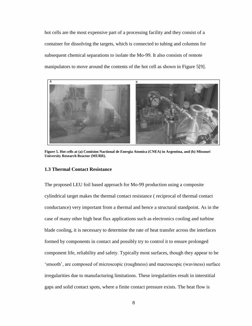
8

hot cells are the most expensive part of a processing facility and they consist of a

container for dissolving the targets, which is connected to tubing and columns for

subsequent chemical separations to isolate the Mo-99. It also consists of remote

manipulators to move around the contents of the hot cell as shown in Figure 5[9].

Figure 5. Hot cells at (a) Comision Nactional de Energia Atomica (CNEA) in Argentina, and (b) Missouri

University Research Reactor (MURR).

1.3 Thermal Contact Resistance

The proposed LEU foil based approach for Mo-99 production using a composite

cylindrical target makes the thermal contact resistance ( reciprocal of thermal contact

conductance) very important from a thermal and hence a structural standpoint. As in the

case of many other high heat flux applications such as electronics cooling and turbine

blade cooling, it is necessary to determine the rate of heat transfer across the interfaces

formed by components in contact and possibly try to control it to ensure prolonged

component life, reliability and safety. Typically most surfaces, though they appear to be

‘smooth’, are composed of microscopic (roughness) and macroscopic (waviness) surface

irregularities due to manufacturing limitations. These irregularities result in interstitial

gaps and solid contact spots, where a finite contact pressure exists. The heat flow is

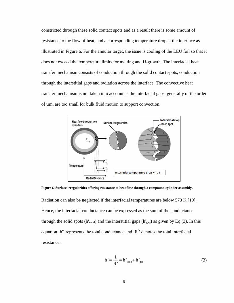
9

constricted through these solid contact spots and as a result there is some amount of

resistance to the flow of heat, and a corresponding temperature drop at the interface as

illustrated in Figure 6. For the annular target, the issue is cooling of the LEU foil so that it

does not exceed the temperature limits for melting and U-growth. The interfacial heat

transfer mechanism consists of conduction through the solid contact spots, conduction

through the interstitial gaps and radiation across the interface. The convective heat

transfer mechanism is not taken into account as the interfacial gaps, generally of the order

of µm, are too small for bulk fluid motion to support convection.

Figure 6. Surface irregularities offering resistance to heat flow through a compound cylinder assembly.

Radiation can also be neglected if the interfacial temperatures are below 573 K [10].

Hence, the interfacial conductance can be expressed as the sum of the conductance

through the solid spots (h'solid) and the interstitial gaps (h'gap) as given by Eq.(3). In this

equation ‘h'’ represents the total conductance and ‘R'’ denotes the total interfacial

resistance.

solid gap

1h ' h ' h '

R ' (3)

10

1.4 Control Blades

The nuclear fission chain reaction is the fundamental process by which nuclear reactors

produce usable energy. In this process, a U-235 atom is struck by an incident neutron,

causing the atom to fission into smaller fragments. These new neutrons then collide with

other U-235 atoms, creating a chain reaction that releases a substantial amount of energy.

Hence the key to sustaining a fission chain reaction is to be able to control the amount of

neutrons that propagate to the subsequent fission step. The control blades are an

important technology for maintaining the desired state of fission reactions within a

nuclear reactor. They help with real time control of the fission process, which is crucial to

keep the fission chain reaction active and prevent it from accelerating beyond control.

The design of a reactor influences the selection of material to be used for control blades.

For the control blade to be able to absorb neutrons, it should have a large neutron

absorption cross section and should be resilient to quick burn out. The material selection

for a control blade is also dependent on the ability of the rod to resonantly absorb

neutrons. Cross sections with this quality are usually preferred over cross sections that

have a high thermal neutron absorption capability [11].

In a nuclear reactor, the reactor core is enclosed by a thick walled cylindrical pressure

vessel. Protecting the inside of the vessel from fast neutrons escaping from the fuel

assembly is a cylindrical shield wrapped around the fuel assembly called the reflector.

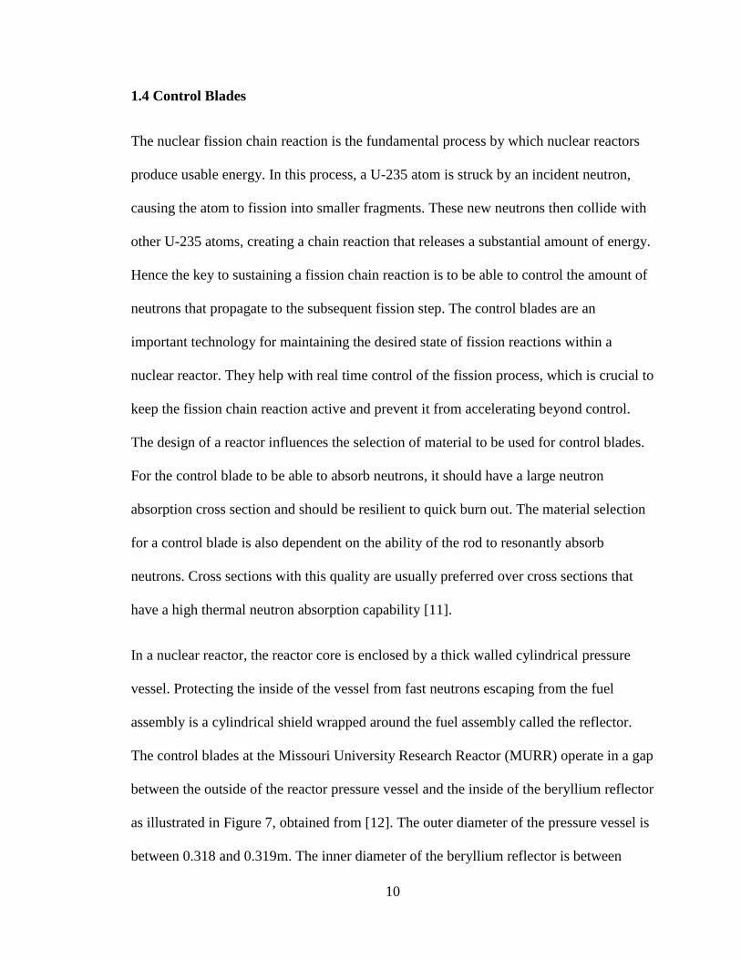
The control blades at the Missouri University Research Reactor (MURR) operate in a gap

between the outside of the reactor pressure vessel and the inside of the beryllium reflector

as illustrated in Figure 7, obtained from [12]. The outer diameter of the pressure vessel is

between 0.318 and 0.319m. The inner diameter of the beryllium reflector is between

11

0.347 and 0.348m. The gap width is maintained by vertical spacers which are set into the

beryllium reflector and cross the gap to the outer diameter of the reactor pressure vessel.

Figure 7. View of the MURR core showing the reflector, control blade and pressure vessel.

The BORAL® control blades used by MURR will experience a thermally induced

deflection during reactor operation due to the composite structure of the control blade.

The neutron absorber in BORAL is boron. BORAL has an aluminum and boron carbide

mixture enclosed in an aluminum cladding. The boron and aluminum mixture (BORAL

meat) and the aluminum cladding are bonded together through powder metallurgy to

establish an adherent bonded plate. As the BORAL absorbs both neutron particles and

gamma rays there is volumetric heat generation and a corresponding rise in temperature.

Since the BORAL meat and the aluminum cladding materials have different thermal

expansion coefficients, the blade may have a tendency to deform as the blade temperature

changes and the materials expand at different rates. In addition to the composite nature of

the control blade, spatial variations in temperature within the control blade occur from the

non-uniform heat generation within the BORAL meat. The high boron-10 cross section

12

of the B-10 (n, α) Li-7 thermal neutron reaction produces the vast majority of the heating

in the control blade. This reaction primarily occurs within the first 0.051 x 10-2

m of the

BORAL meat surface and produces about 2.79 MeV of energy, of which 0.84 MeV is the

reaction energy of the Li-7 and 1.47 MeV is the alpha particle. The remaining 0.48 MeV

is a gamma rays. Hence, about 80 % of the nuclear reaction’s energy is deposited within a

few millimeters of the reaction location. Consequently, the major heating is in the outer

two surfaces of the BORAL meat, making the heat generation through the blade low

except for the outer 0.051 x 10-2

m of each surface. These combine to produce a variation

in the heating profile through the thickness and about the circumferential width of the

control blade. The heat generation is also non-uniform along the longitudinal direction

because the thermal neutron flux drops off significantly from the leading edge (bottom)

of the control blade to the top. Mathematical curve fits are generated for the non-uniform

volumetric heat generation profile caused by the thermal neutron absorption in a B-10 (n,

α) Li-7 reaction and the gamma heating. The functions are applied as heating conditions

within a finite element model of the control blade built using the commercial finite

element code Abaqus FEA. A convective heat transfer coefficient is applied to the outer

boundaries of the control blade and neutral assembly temperature is assumed to be room

temperature. The finite element model is solved as a fully coupled thermal stress analysis,

where the temperature distribution is solved for and then used to determine the

mechanical deflection of the control blade.

1.5 Objective of Work

For the annular target, since most analysis parameters are reactor specific, the goal is to

develop a general performance analysis envelope, using numerical models and simplified

13

analytical expressions for thermal-stresses in composite cylinders, which covers most

operational parameters (heat generation rates, heat transfer coefficients) that are likely to

be used by reactors. The importance of the analysis stems from the fact that, though these

annular targets have been safely irradiated in the past, there is no documented safety

analysis to completely understand the behavior of the targets during irradiation. Hence,

the objective of annular target investigation is to analyze its thermal mechanical behavior,

develop a general performance analysis envelope and assess the conditions under which

the targets could potentially fail.

While the annular target analysis is focused on establishing the magnitude of temperature

and thermally induced stresses in the target, relative to the melting temperature and the

yield strength of the cladding, the goal of the BORAL control blade analysis for MURR

is centered around determining whether the thermally induced deflection of the control

blade will be within the specified channel gap limits for safe operation. The results from

this reactor-specific control blade analysis were used to help MURR with their reactor

relicensing efforts during the summer of 2012. Broadly, it is the thermal-mechanical

behavior of the both these internal heat generating applications that is being analyzed.

Hence, this dissertation will seek to provide analysis results based on two internal heat

generation applications (annular target for Mo-99 production and the control blade

analysis to support MURR relicensing efforts). In both these applications the heat source

is nuclear, there exists high heat flux that needs to be managed by effective cooling, non-

uniform heating, the presence of composite structures and differential thermal expansion,

with the end goal in both these analyses being – component and operational safety.

14

Chapter 2: Literature Review

2.1 Target Design and Irradiations

Low-enriched uranium foil based annular target design and developmental work was

carried out by the Argonne National Lab (ANL) [13]. The design consisted of an LEU

foil sandwiched between concentric cylindrical tubes. A recess was cut on the inner tube

to accommodate the LEU foil. Their analysis focused on developing a cost effective

annular target design that would minimize the thermal contact resistance between the

LEU foil and the target tubes. They performed thermal cycling tests, over a period of 7

days in a furnace at 473 K, on the assembled annular targets and established that they

would perform well when irradiated. They also established the average value of hoop

stress in the outer tube to be 3 MPa. This target design concept was successfully

irradiated in 1999 [14]. Good radiation performance and no heat transfer problems were

reported based on their test results. During disassembly the targets were easily removed

from the irradiation holders and this proved that no significant mechanical distortions

existed during in-pile irradiation. Their conclusions, based on the disassembly, were that

the nickel recoil barriers perform the best while aluminum and zirconium as target tubes

work well.

The thermal mechanical behavior of the LEU foil based annular target developed by [13]

was evaluated by Areva-Cerca [15]. They performed their thermal analysis using the

numerical code CFX and used experiments to determine the thermal contact resistance. In

their experiments they used a perfectly flat rolled LEU foil and did not account for the

surface irregularities (macroscopic and microscopic) on the foil surface which is

15

important in the thermal contact resistance analysis [16]. A feasibility study [17] was

carried out by performing a preliminary thermal and fluid flow analysis to estimate the

heat removal capability for a 20 g LEU foil annular target irradiated in MURR. In the

parametric studies they varied the pressure drop and the thermal load separately. They

concluded that a minimum pressure drop of 15 kPa is required, for a 15 kW heat

dissipation, to ensure that boiling is suppressed. Their thermal load variation studies were

aimed at determining the maximum possible heat dissipation for the target while

maintaining the temperature below 373 K. They concluded that for a uniform heating

configuration, 30 kW heat can be removed before reaching 373 K, and for the non-

uniform heating case, 16 kW heat can be removed before reaching 373 K. Their

parametric studies also helped them conclude that the cladding temperatures for the non-

uniform heating case can be controlled by optimizing the thickness of the aluminum

tubes. The results from the analysis were found to comply with the acceptance criteria

established by the MURR operating licensing technical specifications.

Preliminary safety calculations on a prototype LEU foil based annular target can and

subsequently trials at HIFAR were carried out by the Australian Nuclear Science and

Technology Organization (ANSTO) [18]. In their numerical calculations using CFX4,

they used a 125 micro meter foil, with a target mass of 0.4 g and a thermal neutron flux

of 0.19 E14 n/cm2s. Their analysis predicted a maximum foil temperature of 138

ᵒC and a

maximum can wall temperature of 92ᵒC. They also determined the optimum diameter of

the coolant exit to be 3 mm as it provided greater flow through the inner channel than

through the can-rig channel. This is consistent with the analysis in [17], which also

concluded that there is greater flow through the inner flow channel as compared to the

16

coolant flow between the outer tube and the channel wall. Their trial irradiation results

were also found to be consistent with their numerical analysis results.

A physics study [19], using the neutronics code MCNP, was carried out on the target

irradiation for fission molybdenum production at the High-Flux Advanced Neutron

Application Reactor (HANARO) in Korea. An annulus type of uranium foil (with no

circumferential gap), 100 micro meter in thickness and 100 mm in length was used in the

analysis. The nickel coated uranium foil was sandwiched between two aluminum tubes.

To evaluate the effect of surface roughness, they varied the target foil thickness from 75-

125 micro meters. They found the reactivity change due to loading of targets to be much

lower than that prescribed by the HANARO safety limits. Thermal hydraulic and

neutronics analysis was performed on LEU foil based annular targets for the production

of 100 Ci of molybdenum-99 at the Pakistan research reactor-1 (PARR-1) [20, 21]. They

used a 125 µm thick uranium foil at 19.99 % enrichment, enveloped in a 15 µm thick Ni

foil. This configuration was placed between two aluminum tubes of 162 mm length and

the edges were welded. The reactivity of fission molybdenum-99 was analyzed for

various power levels between 5.4 kW and 17.41 kW. However, for their analysis, they

used the maximum power of 17.41 kW and found the corresponding maximum surface

temperature rise of 317 K to be within the saturation temperature (386 K) at the core

pressure level. Based on their analysis they reported that the reactor safety will not be

compromised in adopting the proposed annular target and holder designs for the

molybdenum-99 production.

Thermal mechanical studies were carried out on LEU foil based flat plate targets by

varying the boundary conditions applied to the aluminum plates [22]. The focus of the

17

analysis was to evaluate the impact of changing boundary conditions (fully constrained,

partially constrained and free) on the thermal mechanical behavior of these plates. They

reported that the variation of stresses and strains induced in the plates was related to the

manner in which the plate was constrained. They also showed that the magnitude of

deflection through the thickness of the plate was greatest when the plate was fully

constrained as opposed to being partially constrained with free edges.

Thermal stress numerical and analytical analyses of annular targets for Mo-99 production

using LEU metal foils have recently been analyzed [23, 24]. In [23] the authors did not

account for the pre stresses from the assembly process. They assumed that their

numerical thermal-mechanical model began from a stress- free state. Their target design

was based on the ANL annular target design [13], but the cladding material was Al 6061-

T6 as compared to the Al 3003-H14 used in [13, 14]. In [24] the authors included the

residual stresses from the hydroforming assembly process and the numerical model was

built to simulate the hydroforming assembly process first, followed by the thermal-

mechanical irradiation analysis. In both these instances [23, 24] they concluded safe

irradiation of these annular targets based on analysis results.

2.2 Thermal Contact Resistance

A good understanding of the interface integrity is an important aspect in high heat flux

applications as the presence of surface irregularities and its incorrect evaluation will

result in overheating and subsequent failure of components. Typically in thermal contact

resistance studies involving flat joints the contact pressure is known and can be taken as

the independent variable. In cylindrical joints, the flow of heat causes the expansion of

18

the tubes which results in the contact pressure [25]. Hence the heat flux is the

independent variable in cylindrical joints.

Results from tests on cylindrical joints with varying interface heat fluxes [26] showed

that the thermal contact resistance is dependent upon the initial gap, the differential

thermal expansion due to an interfacial temperature drop and the differential expansion

due to the temperature gradients. Also, due to the contact resistance being dependent on

the initial gap, the results illustrate that joints with an interference fit will have negligible

thermal contact resistance. This is true as with an interference fit, the interface

temperature discontinuity will be negligible. They also report that the there is a dearth of

literature based on contact conductance studies of cylindrical joints and often the effects

of differential expansion are neglected assuming the thermal contact resistance to be

constant. Power law correlations based on previous experimental work were obtained

[27], to predict the solid spot thermal conductance at the interface of Zircaloy-2 and

Uranium Dioxide. The investigators concluded that more work is required to determine

the effect of mean junction temperature on the thermal contact conductance. They also

stated that the surface parameters other than the roughness effects must be accounted for

future analysis.

Experiments on composite cylinders were performed by Hsu and Tam [28]. They varied

the heat flux, microscopic surface properties only on one side of the interface and

compared their results with those of Ross and Stoute [29]. They found these experimental

results to be much lower than the calculated values and attributed it to the increase in

micro-contact area due to the lateral expansion of the flat contacts and thermally induced

strain at the interface. A study on the coaxial cylindrical casings in a vacuum

19

environment was performed [30], taking into account the mechanical and thermo physical

properties of the tubes. The investigators report a dependency between the contact

pressure, thermal load, initial interference of the tubes and the ratio of thermal expansion

coefficients of the tubes without considering the microscopic or macroscopic surface

irregularities. They concluded that for a case of radially outward heat flow, if the thermal

expansion coefficient of the inner tube is lesser than that of the outer tube then the

thermal contact resistance at the interface will increase due to a decrease in the interfacial

contact pressure.

An iterative procedure [31] was used, based on a plane stress and interference fit

assumption, to predict the contact conductance of cylindrical joints based on flat contact

conductance models. The iterative procedure takes into account the surface roughness,

microhardness and the contact pressure at the interface. The thermal contact conductance

is presented as a function of the contact pressure, thus recommending that accounting for

the difference between the circumferential and axial roughness is important. Their model

was in good agreement with that of Hsu and Tam [28] and the modified flat contact

models of Ross and Stoute [29]. A laser flash technique [32] along with a Gaussian

parameter estimation procedure was employed to estimate the thermal contact resistance

at the interface of a double layer sample. The investigators provide the analysis of

sensitivity coefficients for each parameter of the double-layer sample which can be

extended for use in designing experiments. Based on their numerical simulations they

concluded that their method could estimate the thermal contact resistance between the

layers with high accuracy if any one of the sample materials is a good conductor of heat

or if a thin layer assumption is used. They also found that the energy absorbed by the

20

sample from the laser pulse can be estimated with ease if a high signal to noise ratio

exists. An experimental methodology to predict the thermal contact resistance based on

the interfacial stresses in a pair of concentric aluminum tubes was identified [33]. The

authors showed that for a couple of aluminum tubes in perfect contact, external heating of

the outer tube would result in tensile stresses being generated on both the tubes. This

opens up a gap between the tubes and increases the thermal contact resistance. Internal

heating of the inner tube would result in compressive stresses being generated on the

tubes, thus reducing the thermal contact resistance. Thus by controlling the direction of

heat flow, contact is either established or withdrawn due to the compressive and tensile

stresses respectively.

An expression for the thermal contact conductance (reciprocal of thermal contact

resistance) as a function of the contact pressure, at the interface of Al 6061-T6 and

uranium was recently developed [34]. The expression is based on a widely used

correlation from literature [35] that assumes plastic deformation of the asperities at the

interface. The authors assumed the total conductance to be a sum of the solid spot

conductance and the gap conductance. In the gap conductance calculations, they assumed

that the interstitial gaps would be filled with a mixture of Helium (He), Xenon (Xe),

Krypton (Kr) and Iodine (I). The assumption of the existence of these gases in the

interstitial gaps was made based on the data available from an irradiation study [36].

2.3 Thermal Stresses in Cylinders

Compound cylinders and composite layered structures have a wide range of applications

in gas storage, spacecraft structures, nuclear power plants, nuclear reactor control blades

and also in applications for medical isotope production [24]. Compound cylinders are

21

generally preferred over a single cylinder, as the composite structure provides

reinforcement, thereby increasing its capability to withstand a comparatively larger stress

state. This is especially beneficial in high heat flux applications, such as in nuclear

reactors, where material or component failure due to yielding is undesirable. Over the

years many investigators have come up with steady state and time dependent analytical

solutions for thermal stresses in compound cylinders. The Laplace transform solution

technique has been commonly used to solve the transient problem in compound cylinders

[37] and a single hollow cylinder [38]. The transient thermo elastic solution in compound

cylinders with traction free boundary conditions [37] was solved by utilizing the Laplace

transform and the matrix similarity transform, to obtain a solution that can be applied to

the thermal stress estimation in multilayered composite cylinders with non-homogeneous

materials. The compound cylinders usually undergo an assembly process to fit them

together. This process induces stresses in the material, as a result of which a finite

pressure exists at the interface of the cylinders. The thermal stresses in compound

cylinders with an initial interface pressure have been solved using the finite difference

method in conjunction with the Laplace transform and matrix similarity transform [39].

In compound cylinders with radial heat flow, the thermal expansion coefficient of the

materials, along with the direction of the heat flow dictates the integrity of interfacial

contact [25]. Earlier work [40] also concluded that local separation occurs at the interface

when heat flows into a higher distortivity material. The exact steady state thermo elastic

solution for functionally graded cylinders with the thermal expansion coefficient as a

function of the radius of the cylinder has also been studied [41]. The authors were able to

establish the location of maximum stresses and concluded that the volumetric average of

22

the thermal expansion coefficient can be used to represent the effective thermal

expansion coefficient.

In the nuclear industry there has been an effort to utilize low-enriched uranium metal foil

based annular targets [34] to produce molybdenum-99 and hence obtain its daughter

element technetium-99m which is used as a radioactive tracer. The annular targets used

for this purpose typically consist of a uranium metal foil sandwiched between two

aluminum cylinders to form a composite cylindrical structure [23, 42]. The inner and

outer aluminum cylinders are collectively referred to as the ‘cladding’. Extensive analysis

has been performed in this area using other composite geometries as well [8, 43].

2.4 Fission Gas Release and Uranium Swelling

It has been shown [44, 45] that during irradiation the uranium increases in volume by a

number of mechanisms (increase in atomic volume, low temperature distortion, swelling

by absorption of vacancies and swelling due to fission product gas pressure) each

depending on the irradiation temperature. Most of the available literature [46, 47and 48]

presents the swelling of uranium fuel pins/ rods and there is no available data (to the

knowledge of the author) on swelling of LEU metal foils during irradiation. An available

data source for swelling of pure uranium metal [49] indicates that the swelling due to

irradiation is an integral function of the neutron damage at temperature and time. The

data from this source [49] also indicates that there would be significant swelling at

temperatures in excess of 400ᵒC (673 K) but essentially no swelling at temperatures

below 350ᵒC (623 K). Hence the current approach to address uranium swelling is to

ensure that the LEU temperature remains below 350ᵒC (623 K) at the 100 % power case.

In case the temperatures are found to exceed this value while performing analyses at a

23

higher power (> 100 %), it can be argued that all power ranges above the 100 % power

represent end of the cycle situations and is therefore highly transient, where the reactor

will be scrammed automatically or manually within minutes of the start of the transient.

Irradiation of the LEU foil will produce large amounts of heat along with which fission

by-products are created that include fission gases. The irradiation time dictates the

quantity of gases (number of moles) that are usually generated and released. The noble

gases Xe (Xe-131) and Kr (Kr-84) along with Iodine (I-127) account for the majority of

the fission gases generated [36]. However Iodine release is not expected [50] and only Kr

and Xe are expected to contribute towards the gas release fraction along with He (if the

target was He back filled and the ends were TIG welded). An aspect that needs to be

given consideration is the determination of the volume in which these gases are likely to

be contained. Difficulty arises in determining this volume due to the surface

irregularities. ANSTO in their calculations [18] determined the volume at the elastic limit

and used this value in their fission gas pressure calculations. It is usually assumed that the

gas mixture is ‘ideal’ and the ideal gas law is used to estimate the gas pressure. In their

safety calculations, the gas mixture was assumed to be ideal and a release fraction [51]

was used to determine the fission gas pressure.

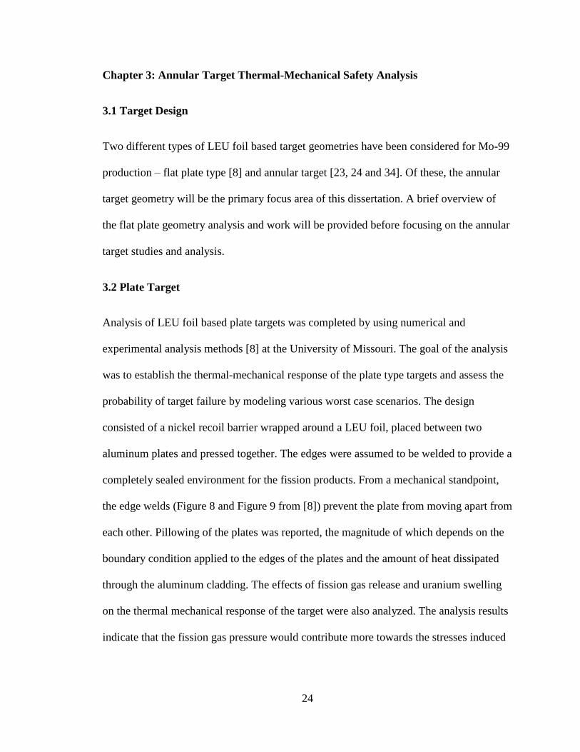
24

Chapter 3: Annular Target Thermal-Mechanical Safety Analysis

3.1 Target Design

Two different types of LEU foil based target geometries have been considered for Mo-99

production – flat plate type [8] and annular target [23, 24 and 34]. Of these, the annular

target geometry will be the primary focus area of this dissertation. A brief overview of

the flat plate geometry analysis and work will be provided before focusing on the annular

target studies and analysis.

3.2 Plate Target

Analysis of LEU foil based plate targets was completed by using numerical and

experimental analysis methods [8] at the University of Missouri. The goal of the analysis

was to establish the thermal-mechanical response of the plate type targets and assess the

probability of target failure by modeling various worst case scenarios. The design

consisted of a nickel recoil barrier wrapped around a LEU foil, placed between two

aluminum plates and pressed together. The edges were assumed to be welded to provide a

completely sealed environment for the fission products. From a mechanical standpoint,

the edge welds (Figure 8 and Figure 9 from [8]) prevent the plate from moving apart from

each other. Pillowing of the plates was reported, the magnitude of which depends on the

boundary condition applied to the edges of the plates and the amount of heat dissipated

through the aluminum cladding. The effects of fission gas release and uranium swelling

on the thermal mechanical response of the target were also analyzed. The analysis results

indicate that the fission gas pressure would contribute more towards the stresses induced

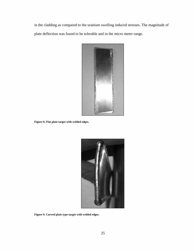
25

in the cladding as compared to the uranium swelling induced stresses. The magnitude of

plate deflection was found to be tolerable and in the micro meter range.

Figure 8. Flat plate target with welded edges.

Figure 9. Curved plate type target with welded edges.

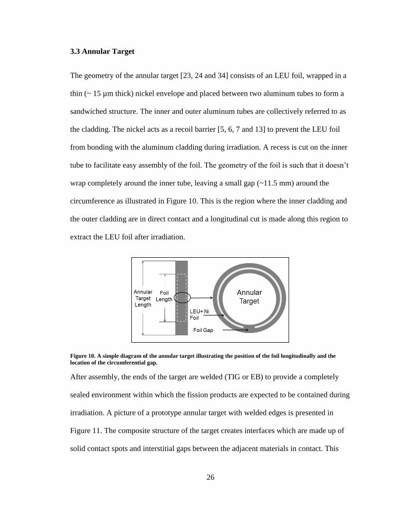
26

3.3 Annular Target

The geometry of the annular target [23, 24 and 34] consists of an LEU foil, wrapped in a

thin (~ 15 µm thick) nickel envelope and placed between two aluminum tubes to form a

sandwiched structure. The inner and outer aluminum tubes are collectively referred to as

the cladding. The nickel acts as a recoil barrier [5, 6, 7 and 13] to prevent the LEU foil

from bonding with the aluminum cladding during irradiation. A recess is cut on the inner

tube to facilitate easy assembly of the foil. The geometry of the foil is such that it doesn’t

wrap completely around the inner tube, leaving a small gap (~11.5 mm) around the

circumference as illustrated in Figure 10. This is the region where the inner cladding and

the outer cladding are in direct contact and a longitudinal cut is made along this region to

extract the LEU foil after irradiation.

Figure 10. A simple diagram of the annular target illustrating the position of the foil longitudinally and the

location of the circumferential gap.

After assembly, the ends of the target are welded (TIG or EB) to provide a completely

sealed environment within which the fission products are expected to be contained during

irradiation. A picture of a prototype annular target with welded edges is presented in

Figure 11. The composite structure of the target creates interfaces which are made up of

solid contact spots and interstitial gaps between the adjacent materials in contact. This

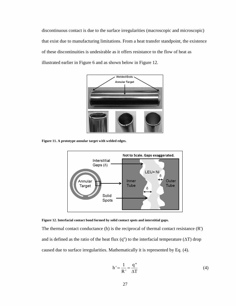
27

discontinuous contact is due to the surface irregularities (macroscopic and microscopic)

that exist due to manufacturing limitations. From a heat transfer standpoint, the existence

of these discontinuities is undesirable as it offers resistance to the flow of heat as

illustrated earlier in Figure 6 and as shown below in Figure 12.

Figure 11. A prototype annular target with welded edges.

Figure 12. Interfacial contact bond formed by solid contact spots and interstitial gaps.

The thermal contact conductance (h) is the reciprocal of thermal contact resistance (R')

and is defined as the ratio of the heat flux (q'') to the interfacial temperature (ΔT) drop

caused due to surface irregularities. Mathematically it is represented by Eq. (4).

1 q ''

h 'R ' T

(4)

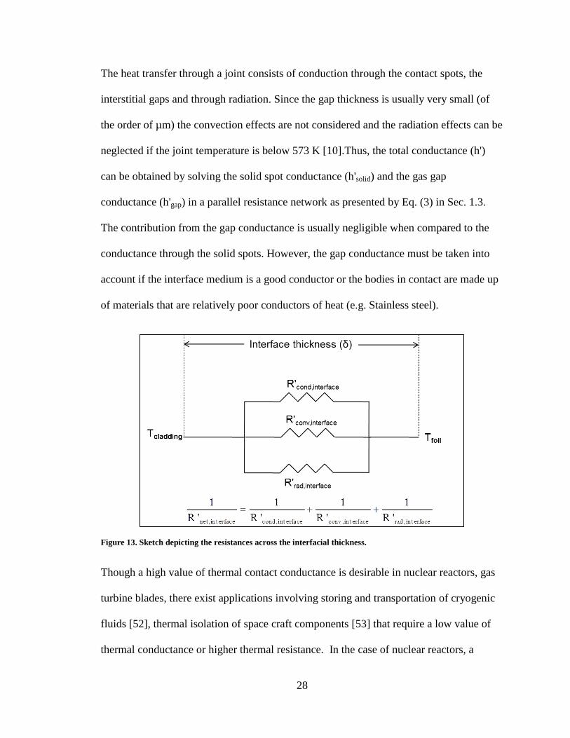
28

The heat transfer through a joint consists of conduction through the contact spots, the

interstitial gaps and through radiation. Since the gap thickness is usually very small (of

the order of µm) the convection effects are not considered and the radiation effects can be

neglected if the joint temperature is below 573 K [10].Thus, the total conductance (h')

can be obtained by solving the solid spot conductance (h'solid) and the gas gap

conductance (h'gap) in a parallel resistance network as presented by Eq. (3) in Sec. 1.3.

The contribution from the gap conductance is usually negligible when compared to the

conductance through the solid spots. However, the gap conductance must be taken into

account if the interface medium is a good conductor or the bodies in contact are made up

of materials that are relatively poor conductors of heat (e.g. Stainless steel).

Figure 13. Sketch depicting the resistances across the interfacial thickness.

Though a high value of thermal contact conductance is desirable in nuclear reactors, gas

turbine blades, there exist applications involving storing and transportation of cryogenic

fluids [52], thermal isolation of space craft components [53] that require a low value of

thermal conductance or higher thermal resistance. In the case of nuclear reactors, a

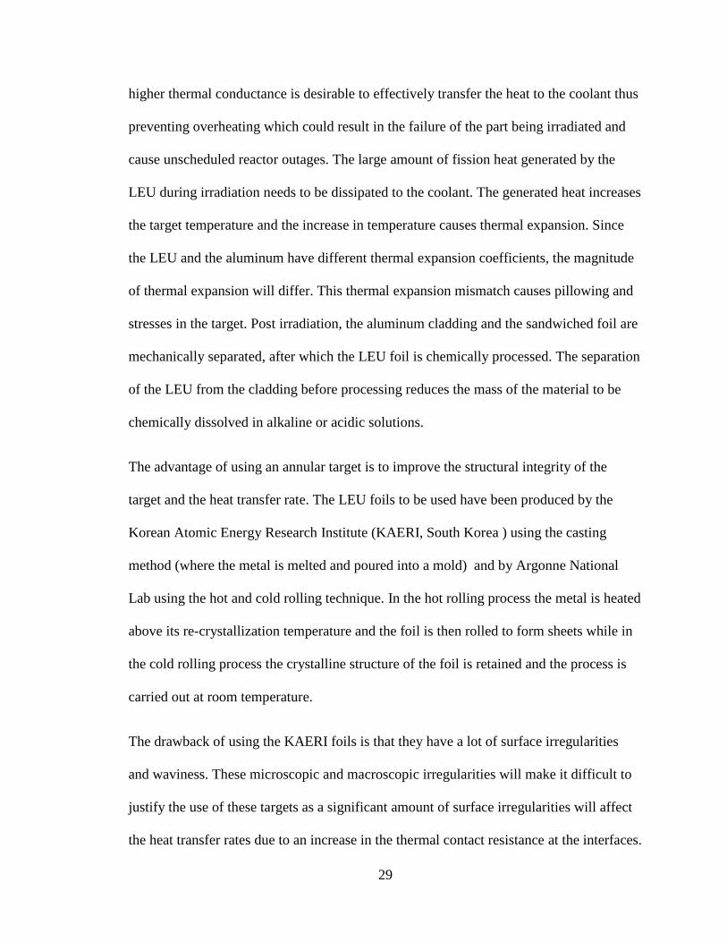
29

higher thermal conductance is desirable to effectively transfer the heat to the coolant thus

preventing overheating which could result in the failure of the part being irradiated and

cause unscheduled reactor outages. The large amount of fission heat generated by the

LEU during irradiation needs to be dissipated to the coolant. The generated heat increases

the target temperature and the increase in temperature causes thermal expansion. Since

the LEU and the aluminum have different thermal expansion coefficients, the magnitude

of thermal expansion will differ. This thermal expansion mismatch causes pillowing and

stresses in the target. Post irradiation, the aluminum cladding and the sandwiched foil are

mechanically separated, after which the LEU foil is chemically processed. The separation

of the LEU from the cladding before processing reduces the mass of the material to be

chemically dissolved in alkaline or acidic solutions.

The advantage of using an annular target is to improve the structural integrity of the

target and the heat transfer rate. The LEU foils to be used have been produced by the

Korean Atomic Energy Research Institute (KAERI, South Korea ) using the casting

method (where the metal is melted and poured into a mold) and by Argonne National

Lab using the hot and cold rolling technique. In the hot rolling process the metal is heated

above its re-crystallization temperature and the foil is then rolled to form sheets while in

the cold rolling process the crystalline structure of the foil is retained and the process is

carried out at room temperature.

The drawback of using the KAERI foils is that they have a lot of surface irregularities

and waviness. These microscopic and macroscopic irregularities will make it difficult to

justify the use of these targets as a significant amount of surface irregularities will affect

the heat transfer rates due to an increase in the thermal contact resistance at the interfaces.

30

The cold rolling technique used by the Argonne National Lab, though an expensive and

labor intensive method can eliminate the surface irregularities. The annular target design

[54] used by the Missouri University Research Reactor (MURR) is presented in the

Figure 14. It should be noted that the choice of cladding material for this target presented

in Figure 14 is Al 3003-H14, but the current analysis considers Al 6061-T6 to be the

cladding material. Aluminum alloy 6061-T6 has higher material yield strength (276 MPa)

as compared to Al 3003-H14 (145 MPa).

Figure 14. Annular target design using Al 3003-H14 as the cladding with the dimensions.

31

Chapter 4: Modeling Without Residual Stresses

Prior to being irradiated in a nuclear reactor, the annular targets undergo ‘preparation’.

This preparation involves assembling the targets [24, 55] and welding the target ends.

The assembly process induces residual stresses in the target and these residual stresses

remain in the target prior to irradiation. The initial part of the analysis does not account

for the residual stresses in the thermal-mechanical irradiation modeling and all the

analysis in Sec 4 and its sub-sections will provide analysis and results without the effects

of the assembly residual stresses. The analysis results with the residual stresses will be

presented in detail in Sec. 7 and its sub-sections.

The commercial finite element code Abaqus FEA [56], version 6.10, was used to perform

a thermal-mechanical analysis on the annular foil based target. Originally released in the

year 1978, Abaqus FEA is a set of software applications meant for finite element analysis

and computer aided engineering. A numerical simulation in Abaqus FEA typically

consists of 3 separate stages namely the pre-processing stage, simulation evaluation stage

and the post processing stage. The pre-processing stage involves creation of an input file

which contains all the constraints under which the model is to be numerically evaluated.

In the second stage the numerical analysis is evaluated based on the constraints specified

in the pre-processing stage or the Abaqus FEA input file. The post-processing stage

involves visualizing the results and extracting data.

4.1 Non-Uniform Heating Numerical Model

Since running full blown 3D finite element simulations is time consuming and not cost

effective, it was decided to simplify the analysis and create a 2D model of the heated

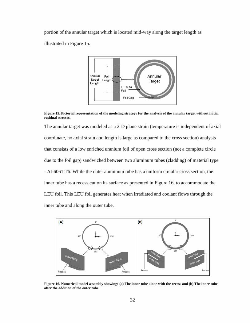
32

portion of the annular target which is located mid-way along the target length as

illustrated in Figure 15.

Figure 15. Pictorial representation of the modeling strategy for the analysis of the annular target without initial

residual stresses.

The annular target was modeled as a 2-D plane strain (temperature is independent of axial

coordinate, no axial strain and length is large as compared to the cross section) analysis

that consists of a low enriched uranium foil of open cross section (not a complete circle

due to the foil gap) sandwiched between two aluminum tubes (cladding) of material type

- Al-6061 T6. While the outer aluminum tube has a uniform circular cross section, the

inner tube has a recess cut on its surface as presented in Figure 16, to accommodate the

LEU foil. This LEU foil generates heat when irradiated and coolant flows through the

inner tube and along the outer tube.

Figure 16. Numerical model assembly showing: (a) The inner tube alone with the recess and (b) The inner tube

after the addition of the outer tube.

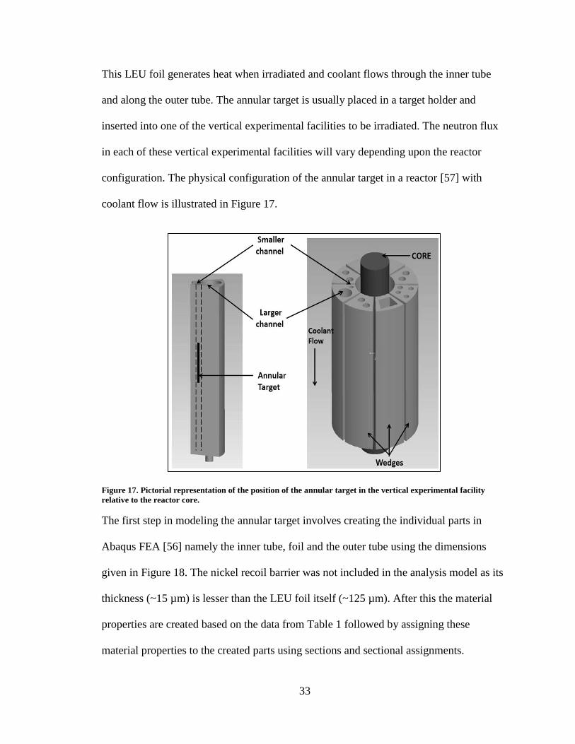
33

This LEU foil generates heat when irradiated and coolant flows through the inner tube

and along the outer tube. The annular target is usually placed in a target holder and

inserted into one of the vertical experimental facilities to be irradiated. The neutron flux

in each of these vertical experimental facilities will vary depending upon the reactor

configuration. The physical configuration of the annular target in a reactor [57] with

coolant flow is illustrated in Figure 17.

Figure 17. Pictorial representation of the position of the annular target in the vertical experimental facility

relative to the reactor core.

The first step in modeling the annular target involves creating the individual parts in

Abaqus FEA [56] namely the inner tube, foil and the outer tube using the dimensions

given in Figure 18. The nickel recoil barrier was not included in the analysis model as its

thickness (~15 µm) is lesser than the LEU foil itself (~125 µm). After this the material

properties are created based on the data from Table 1 followed by assigning these

material properties to the created parts using sections and sectional assignments.

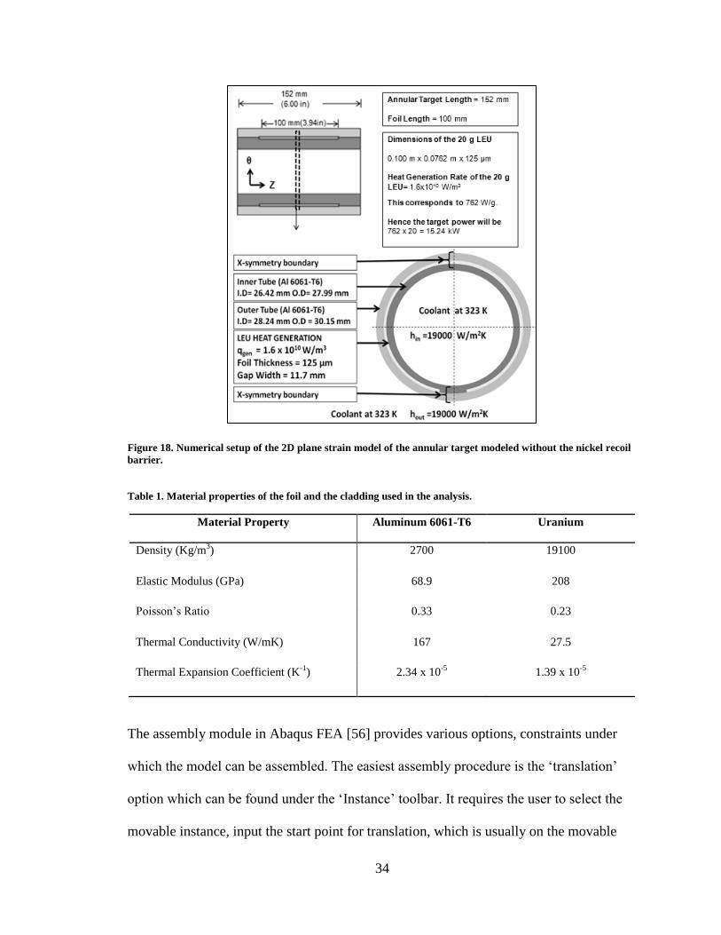
34

Figure 18. Numerical setup of the 2D plane strain model of the annular target modeled without the nickel recoil

barrier.

Table 1. Material properties of the foil and the cladding used in the analysis.

Material Property Aluminum 6061-T6 Uranium

Density (Kg/m3) 2700 19100

Elastic Modulus (GPa) 68.9 208

Poisson’s Ratio 0.33 0.23

Thermal Conductivity (W/mK) 167 27.5

Thermal Expansion Coefficient (K-1

) 2.34 x 10-5

1.39 x 10-5

The assembly module in Abaqus FEA [56] provides various options, constraints under

which the model can be assembled. The easiest assembly procedure is the ‘translation’

option which can be found under the ‘Instance’ toolbar. It requires the user to select the

movable instance, input the start point for translation, which is usually on the movable

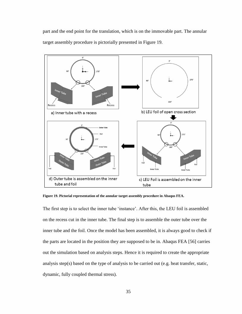
35

part and the end point for the translation, which is on the immovable part. The annular

target assembly procedure is pictorially presented in Figure 19.

Figure 19. Pictorial representation of the annular target assembly procedure in Abaqus FEA.

The first step is to select the inner tube ‘instance’. After this, the LEU foil is assembled

on the recess cut in the inner tube. The final step is to assemble the outer tube over the

inner tube and the foil. Once the model has been assembled, it is always good to check if

the parts are located in the position they are supposed to be in. Abaqus FEA [56] carries

out the simulation based on analysis steps. Hence it is required to create the appropriate

analysis step(s) based on the type of analysis to be carried out (e.g. heat transfer, static,

dynamic, fully coupled thermal stress).

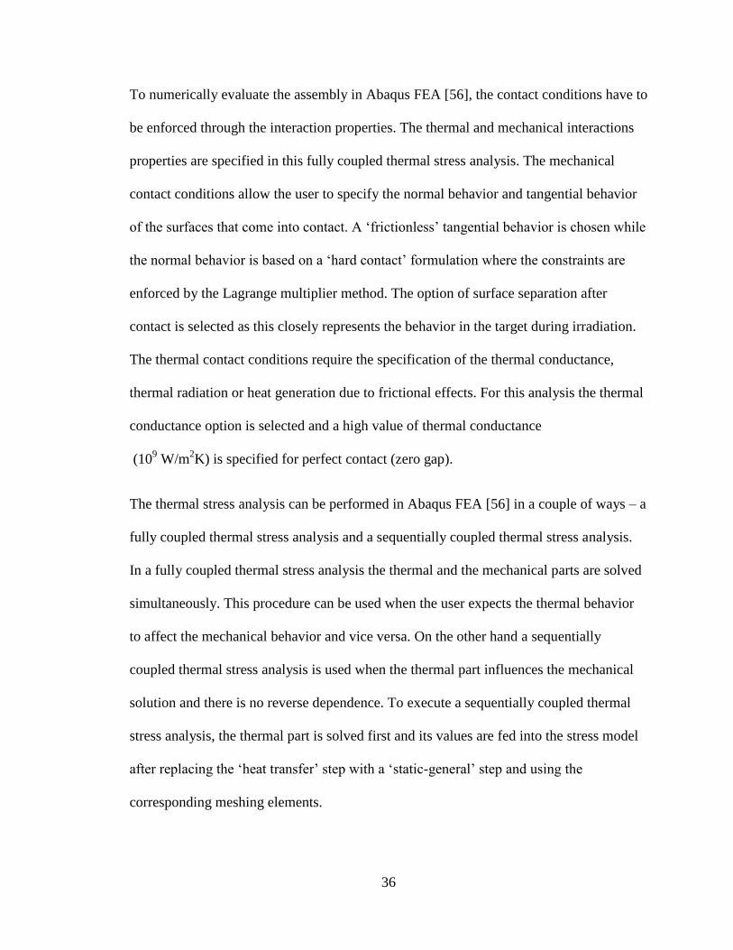
36

To numerically evaluate the assembly in Abaqus FEA [56], the contact conditions have to

be enforced through the interaction properties. The thermal and mechanical interactions

properties are specified in this fully coupled thermal stress analysis. The mechanical

contact conditions allow the user to specify the normal behavior and tangential behavior

of the surfaces that come into contact. A ‘frictionless’ tangential behavior is chosen while

the normal behavior is based on a ‘hard contact’ formulation where the constraints are

enforced by the Lagrange multiplier method. The option of surface separation after

contact is selected as this closely represents the behavior in the target during irradiation.

The thermal contact conditions require the specification of the thermal conductance,

thermal radiation or heat generation due to frictional effects. For this analysis the thermal

conductance option is selected and a high value of thermal conductance

(109 W/m

2K) is specified for perfect contact (zero gap).

The thermal stress analysis can be performed in Abaqus FEA [56] in a couple of ways – a

fully coupled thermal stress analysis and a sequentially coupled thermal stress analysis.

In a fully coupled thermal stress analysis the thermal and the mechanical parts are solved

simultaneously. This procedure can be used when the user expects the thermal behavior

to affect the mechanical behavior and vice versa. On the other hand a sequentially

coupled thermal stress analysis is used when the thermal part influences the mechanical

solution and there is no reverse dependence. To execute a sequentially coupled thermal

stress analysis, the thermal part is solved first and its values are fed into the stress model

after replacing the ‘heat transfer’ step with a ‘static-general’ step and using the

corresponding meshing elements.

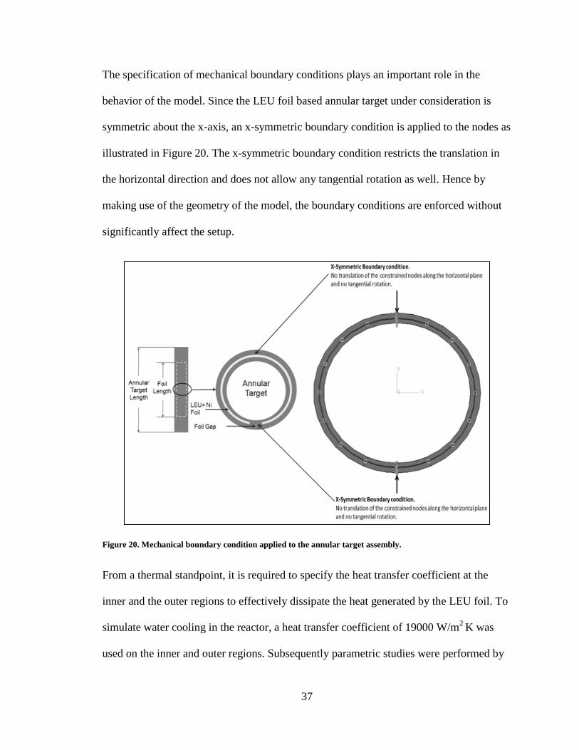
37

The specification of mechanical boundary conditions plays an important role in the

behavior of the model. Since the LEU foil based annular target under consideration is

symmetric about the x-axis, an x-symmetric boundary condition is applied to the nodes as

illustrated in Figure 20. The x-symmetric boundary condition restricts the translation in

the horizontal direction and does not allow any tangential rotation as well. Hence by

making use of the geometry of the model, the boundary conditions are enforced without

significantly affect the setup.

Figure 20. Mechanical boundary condition applied to the annular target assembly.

From a thermal standpoint, it is required to specify the heat transfer coefficient at the

inner and the outer regions to effectively dissipate the heat generated by the LEU foil. To

simulate water cooling in the reactor, a heat transfer coefficient of 19000 W/m2

K was

used on the inner and outer regions. Subsequently parametric studies were performed by

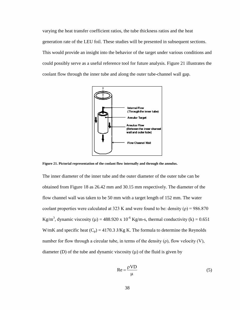
38

varying the heat transfer coefficient ratios, the tube thickness ratios and the heat

generation rate of the LEU foil. These studies will be presented in subsequent sections.

This would provide an insight into the behavior of the target under various conditions and

could possibly serve as a useful reference tool for future analysis. Figure 21 illustrates the

coolant flow through the inner tube and along the outer tube-channel wall gap.

Figure 21. Pictorial representation of the coolant flow internally and through the annulus.

The inner diameter of the inner tube and the outer diameter of the outer tube can be

obtained from Figure 18 as 26.42 mm and 30.15 mm respectively. The diameter of the

flow channel wall was taken to be 50 mm with a target length of 152 mm. The water

coolant properties were calculated at 323 K and were found to be: density (ρ) = 986.870

Kg/m3, dynamic viscosity (µ) = 488.920 x 10

-6 Kg/m-s, thermal conductivity (k) = 0.651

W/mK and specific heat (Cp) = 4170.3 J/Kg K. The formula to determine the Reynolds

number for flow through a circular tube, in terms of the density (ρ), flow velocity (V),

diameter (D) of the tube and dynamic viscosity (µ) of the fluid is given by

VD

Re

(5)

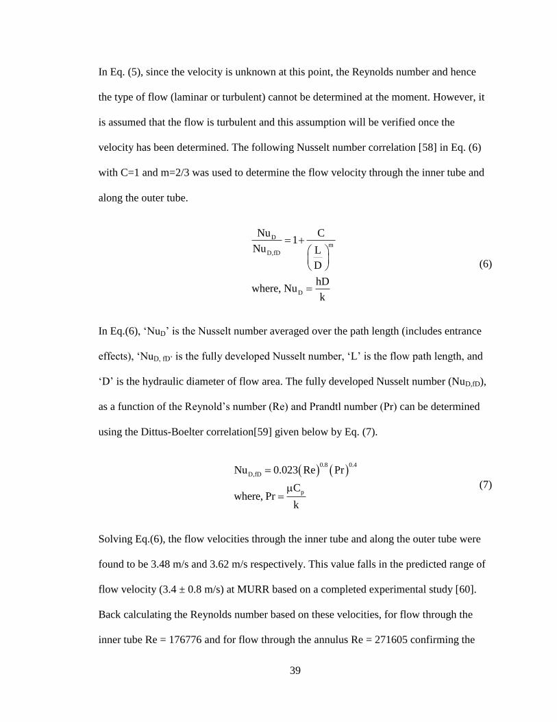
39

In Eq. (5), since the velocity is unknown at this point, the Reynolds number and hence

the type of flow (laminar or turbulent) cannot be determined at the moment. However, it

is assumed that the flow is turbulent and this assumption will be verified once the

velocity has been determined. The following Nusselt number correlation [58] in Eq. (6)

with C=1 and m=2/3 was used to determine the flow velocity through the inner tube and

along the outer tube.

D

m

D,fD

D

Nu C1

Nu L

D

hDwhere, Nu

k

(6)

In Eq.(6), ‘NuD’ is the Nusselt number averaged over the path length (includes entrance

effects), ‘NuD, fD’ is the fully developed Nusselt number, ‘L’ is the flow path length, and

‘D’ is the hydraulic diameter of flow area. The fully developed Nusselt number (NuD,fD),

as a function of the Reynold’s number (Re) and Prandtl number (Pr) can be determined

using the Dittus-Boelter correlation[59] given below by Eq. (7).

0.8 0.4

D,fD

p

Nu 0.023 Re Pr

Cwhere, Pr

k

(7)

Solving Eq.(6), the flow velocities through the inner tube and along the outer tube were

found to be 3.48 m/s and 3.62 m/s respectively. This value falls in the predicted range of

flow velocity (3.4 ± 0.8 m/s) at MURR based on a completed experimental study [60].

Back calculating the Reynolds number based on these velocities, for flow through the

inner tube Re = 176776 and for flow through the annulus Re = 271605 confirming the

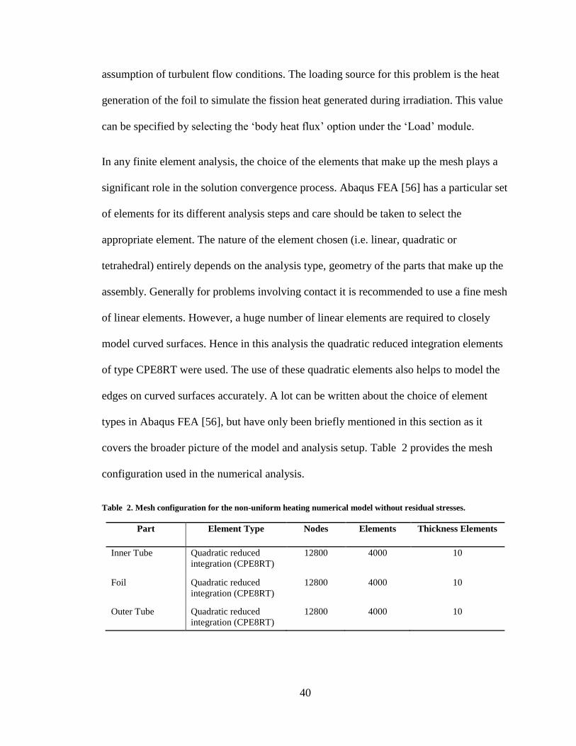
40

assumption of turbulent flow conditions. The loading source for this problem is the heat

generation of the foil to simulate the fission heat generated during irradiation. This value

can be specified by selecting the ‘body heat flux’ option under the ‘Load’ module.

In any finite element analysis, the choice of the elements that make up the mesh plays a

significant role in the solution convergence process. Abaqus FEA [56] has a particular set

of elements for its different analysis steps and care should be taken to select the

appropriate element. The nature of the element chosen (i.e. linear, quadratic or

tetrahedral) entirely depends on the analysis type, geometry of the parts that make up the

assembly. Generally for problems involving contact it is recommended to use a fine mesh

of linear elements. However, a huge number of linear elements are required to closely

model curved surfaces. Hence in this analysis the quadratic reduced integration elements

of type CPE8RT were used. The use of these quadratic elements also helps to model the

edges on curved surfaces accurately. A lot can be written about the choice of element

types in Abaqus FEA [56], but have only been briefly mentioned in this section as it

covers the broader picture of the model and analysis setup. Table 2 provides the mesh

configuration used in the numerical analysis.

Table 2. Mesh configuration for the non-uniform heating numerical model without residual stresses.

Part Element Type Nodes Elements Thickness Elements

Inner Tube Quadratic reduced

integration (CPE8RT)

12800 4000 10

Foil Quadratic reduced


12800 4000 10

Outer Tube Quadratic reduced


12800 4000 10

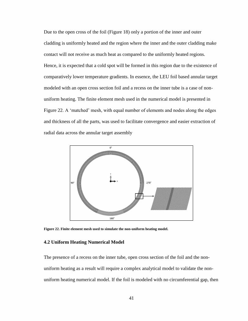
41

Due to the open cross of the foil (Figure 18) only a portion of the inner and outer

cladding is uniformly heated and the region where the inner and the outer cladding make

contact will not receive as much heat as compared to the uniformly heated regions.

Hence, it is expected that a cold spot will be formed in this region due to the existence of

comparatively lower temperature gradients. In essence, the LEU foil based annular target

modeled with an open cross section foil and a recess on the inner tube is a case of non-

uniform heating. The finite element mesh used in the numerical model is presented in

Figure 22. A ‘matched’ mesh, with equal number of elements and nodes along the edges

and thickness of all the parts, was used to facilitate convergence and easier extraction of

radial data across the annular target assembly

Figure 22. Finite element mesh used to simulate the non-uniform heating model.

4.2 Uniform Heating Numerical Model

The presence of a recess on the inner tube, open cross section of the foil and the non-

uniform heating as a result will require a complex analytical model to validate the non-

uniform heating numerical model. If the foil is modeled with no circumferential gap, then

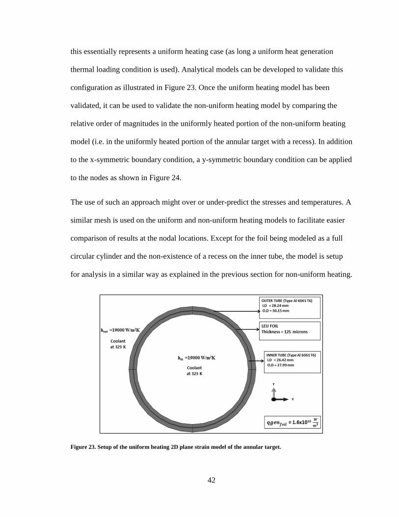
42

this essentially represents a uniform heating case (as long a uniform heat generation

thermal loading condition is used). Analytical models can be developed to validate this

configuration as illustrated in Figure 23. Once the uniform heating model has been

validated, it can be used to validate the non-uniform heating model by comparing the

relative order of magnitudes in the uniformly heated portion of the non-uniform heating

model (i.e. in the uniformly heated portion of the annular target with a recess). In addition

to the x-symmetric boundary condition, a y-symmetric boundary condition can be applied

to the nodes as shown in Figure 24.

The use of such an approach might over or under-predict the stresses and temperatures. A

similar mesh is used on the uniform and non-uniform heating models to facilitate easier

comparison of results at the nodal locations. Except for the foil being modeled as a full

circular cylinder and the non-existence of a recess on the inner tube, the model is setup

for analysis in a similar way as explained in the previous section for non-uniform heating.

Figure 23. Setup of the uniform heating 2D plane strain model of the annular target.

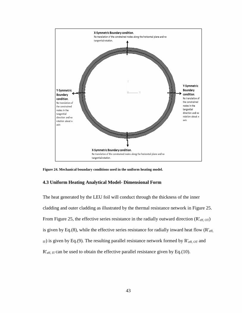
43

Figure 24. Mechanical boundary conditions used in the uniform heating model.

4.3 Uniform Heating Analytical Model- Dimensional Form

The heat generated by the LEU foil will conduct through the thickness of the inner

cladding and outer cladding as illustrated by the thermal resistance network in Figure 25.

From Figure 25, the effective series resistance in the radially outward direction (R'eff, OT)

is given by Eq.(8), while the effective series resistance for radially inward heat flow (R'eff,

IT) is given by Eq.(9). The resulting parallel resistance network formed by R'eff, OT and

R'eff, IT can be used to obtain the effective parallel resistance given by Eq.(10).

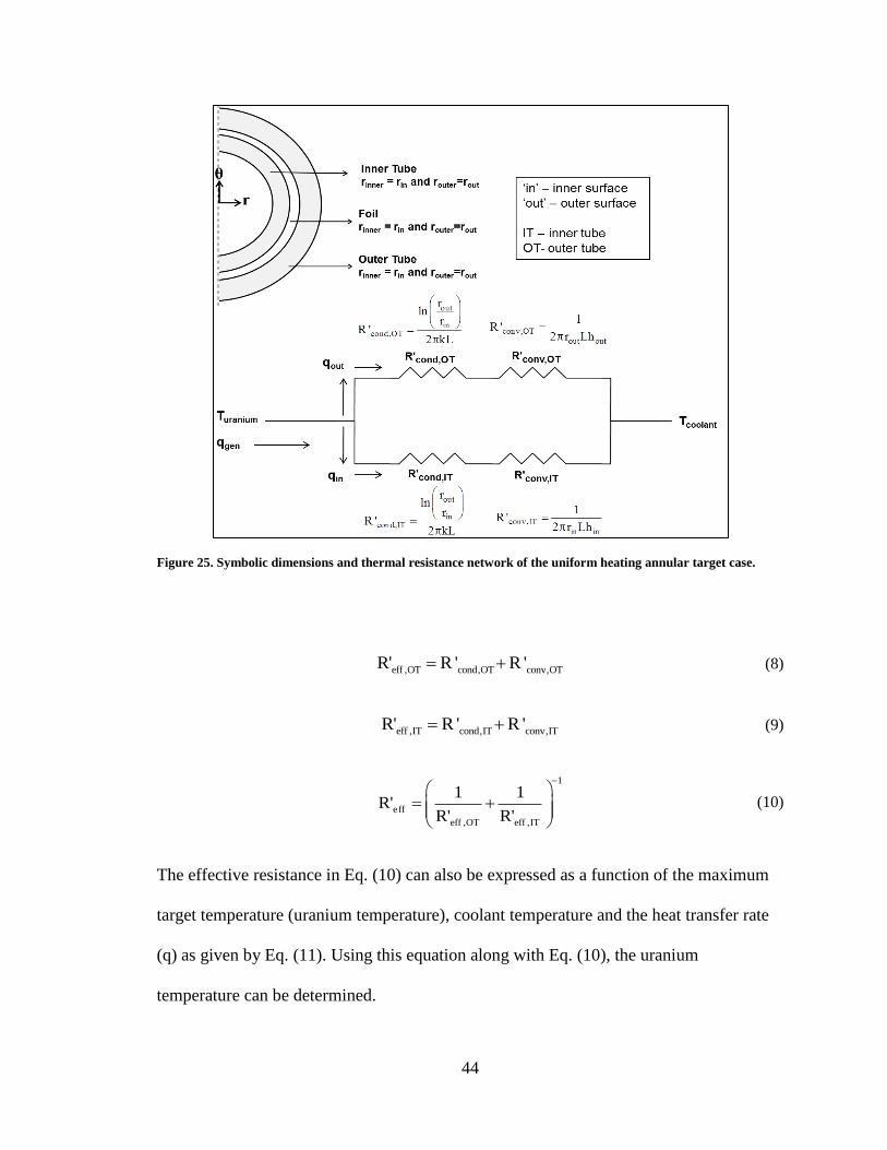
44

Figure 25. Symbolic dimensions and thermal resistance network of the uniform heating annular target case.

eff ,OT cond,OT conv,OTR' R ' R ' (8)

eff ,IT cond,IT conv,ITR' R ' R ' (9)

1

eff

eff ,OT eff ,IT

1 1R'

R' R'

(10)

The effective resistance in Eq. (10) can also be expressed as a function of the maximum

target temperature (uranium temperature), coolant temperature and the heat transfer rate

(q) as given by Eq. (11). Using this equation along with Eq. (10), the uranium

temperature can be determined.

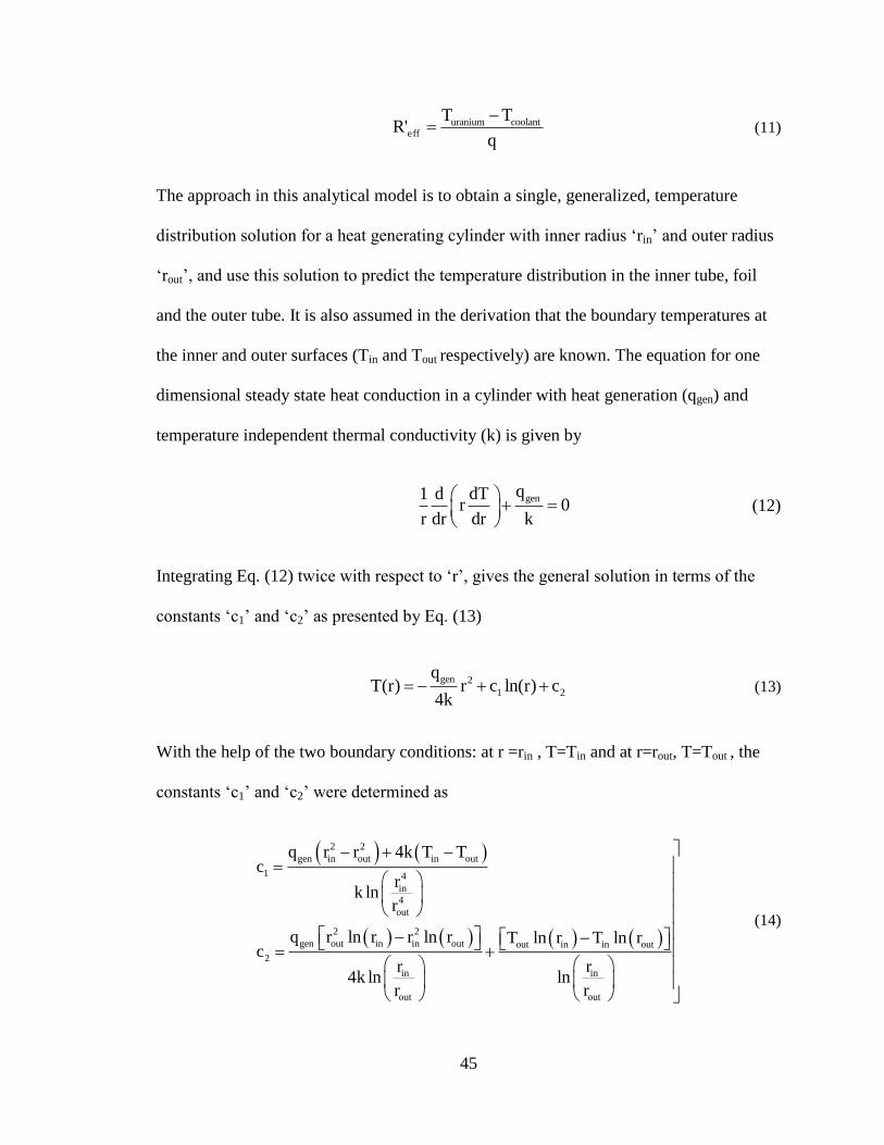
45

uranium coolanteff

T TR'

q

(11)

The approach in this analytical model is to obtain a single, generalized, temperature

distribution solution for a heat generating cylinder with inner radius ‘rin’ and outer radius

‘rout’, and use this solution to predict the temperature distribution in the inner tube, foil

and the outer tube. It is also assumed in the derivation that the boundary temperatures at

the inner and outer surfaces (Tin and Tout respectively) are known. The equation for one

dimensional steady state heat conduction in a cylinder with heat generation (qgen) and

temperature independent thermal conductivity (k) is given by

genq1 d dTr 0

r dr dr k

(12)

Integrating Eq. (12) twice with respect to ‘r’, gives the general solution in terms of the

constants ‘c1’ and ‘c2’ as presented by Eq. (13)

gen 2

1 2

qT(r) r c ln(r) c

4k (13)

With the help of the two boundary conditions: at r =rin , T=Tin and at r=rout, T=Tout , the

constants ‘c1’ and ‘c2’ were determined as

2 2

gen in out in out

1 4

in

4

out

2 2

gen out in in out out in in out

2

in in

out out

q r r 4k T Tc

rk ln

r

q r ln r r ln r T ln r T ln rc

r r4k ln ln

r r

(14)

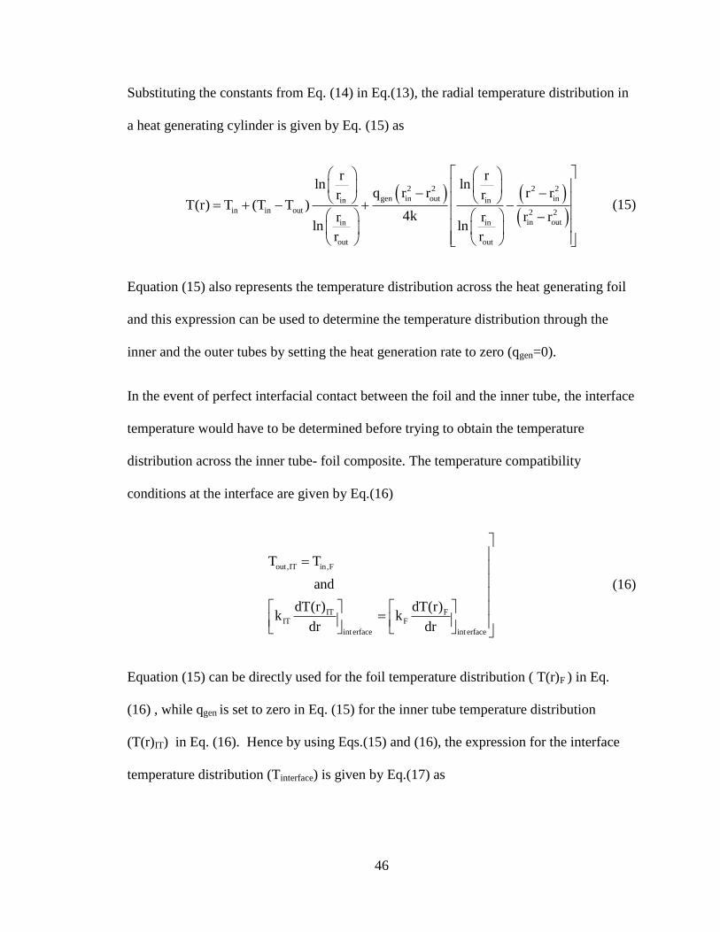
46

Substituting the constants from Eq. (14) in Eq.(13), the radial temperature distribution in

a heat generating cylinder is given by Eq. (15) as

2 2 2 2

gen in out inin in

in in out 2 2

in outin in

out out

r rln ln

q r r r rr rT(r) T (T T )

4k r rr rln ln

r r

(15)

Equation (15) also represents the temperature distribution across the heat generating foil

and this expression can be used to determine the temperature distribution through the

inner and the outer tubes by setting the heat generation rate to zero (qgen=0).

In the event of perfect interfacial contact between the foil and the inner tube, the interface

temperature would have to be determined before trying to obtain the temperature

distribution across the inner tube- foil composite. The temperature compatibility

conditions at the interface are given by Eq.(16)

out,IT in,F

IT FIT F

int erface int erface

T T

and

dT(r) dT(r)k k

dr dr

(16)

Equation (15) can be directly used for the foil temperature distribution ( T(r)F ) in Eq.

(16) , while qgen is set to zero in Eq. (15) for the inner tube temperature distribution

(T(r)IT) in Eq. (16). Hence by using Eqs.(15) and (16), the expression for the interface

temperature distribution (Tinterface) is given by Eq.(17) as

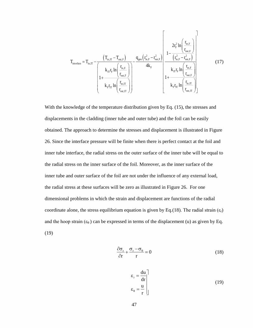
47

in,F2

F

out,F

2 2 2 2

gen in,F out,F in,F out,Fin,IT out,F

int erface in,IT

F in,Fin,FIT FIT F

out,Fout,F

in,ITF ITF IT

out,IT

r2r ln

r1

q r r r rT TT T

4k rrk r lnk r ln

rr11

rrk r lnk r ln

r

in,IT

out,ITr

(17)

With the knowledge of the temperature distribution given by Eq. (15), the stresses and

displacements in the cladding (inner tube and outer tube) and the foil can be easily

obtained. The approach to determine the stresses and displacement is illustrated in Figure

26. Since the interface pressure will be finite when there is perfect contact at the foil and

inner tube interface, the radial stress on the outer surface of the inner tube will be equal to

the radial stress on the inner surface of the foil. Moreover, as the inner surface of the

inner tube and outer surface of the foil are not under the influence of any external load,

the radial stress at these surfaces will be zero as illustrated in Figure 26. For one

dimensional problems in which the strain and displacement are functions of the radial

coordinate alone, the stress equilibrium equation is given by Eq.(18). The radial strain (εr)

and the hoop strain (εθ ) can be expressed in terms of the displacement (u) as given by Eq.

(19)

rr 0r r

(18)

r

du

dr

u

r

(19)

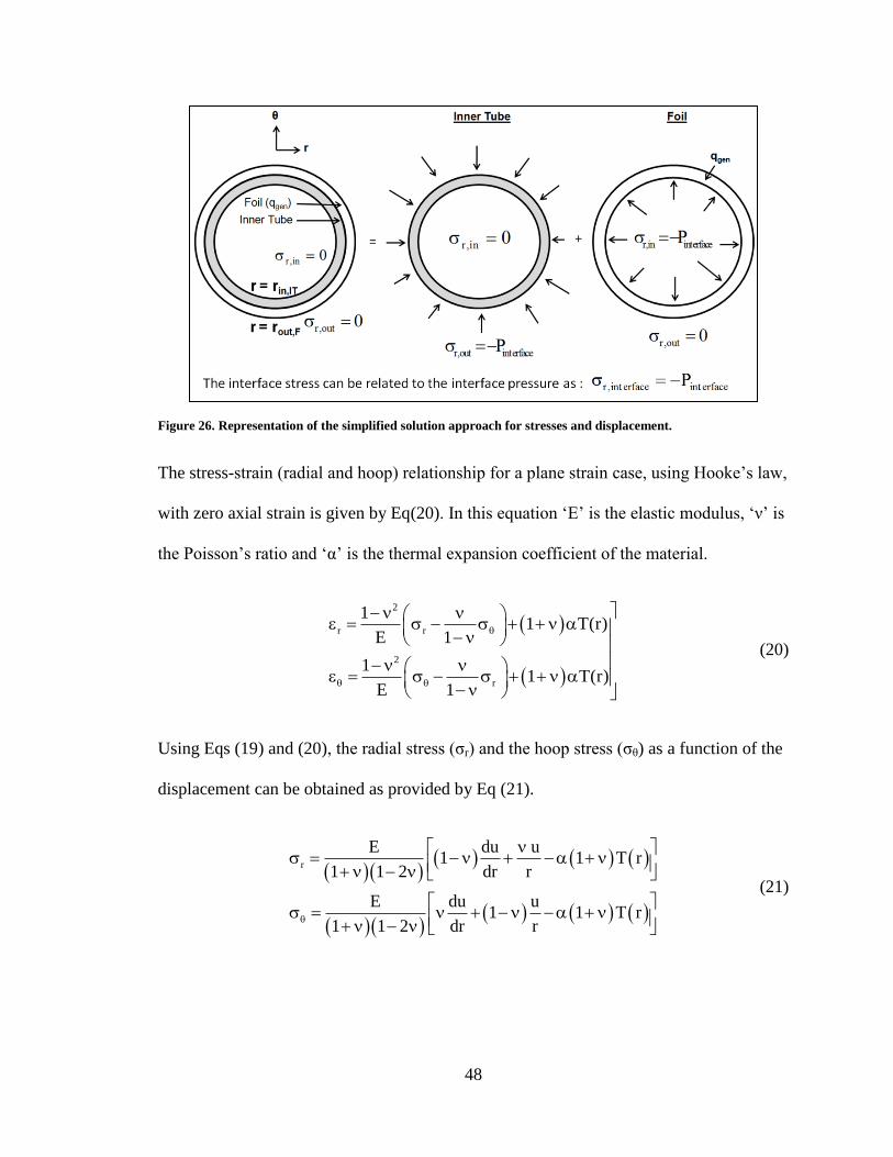
48

Figure 26. Representation of the simplified solution approach for stresses and displacement.

The stress-strain (radial and hoop) relationship for a plane strain case, using Hooke’s law,

with zero axial strain is given by Eq(20). In this equation ‘E’ is the elastic modulus, ‘ν’ is

the Poisson’s ratio and ‘α’ is the thermal expansion coefficient of the material.

2

r r

2

r

11 T(r)

E 1

11 T(r)

E 1

(20)

Using Eqs (19) and (20), the radial stress (σr) and the hoop stress (σθ) as a function of the

displacement can be obtained as provided by Eq (21).

r

E du u1 1 T r

1 1 2 dr r

E du u1 1 T r

1 1 2 dr r

(21)

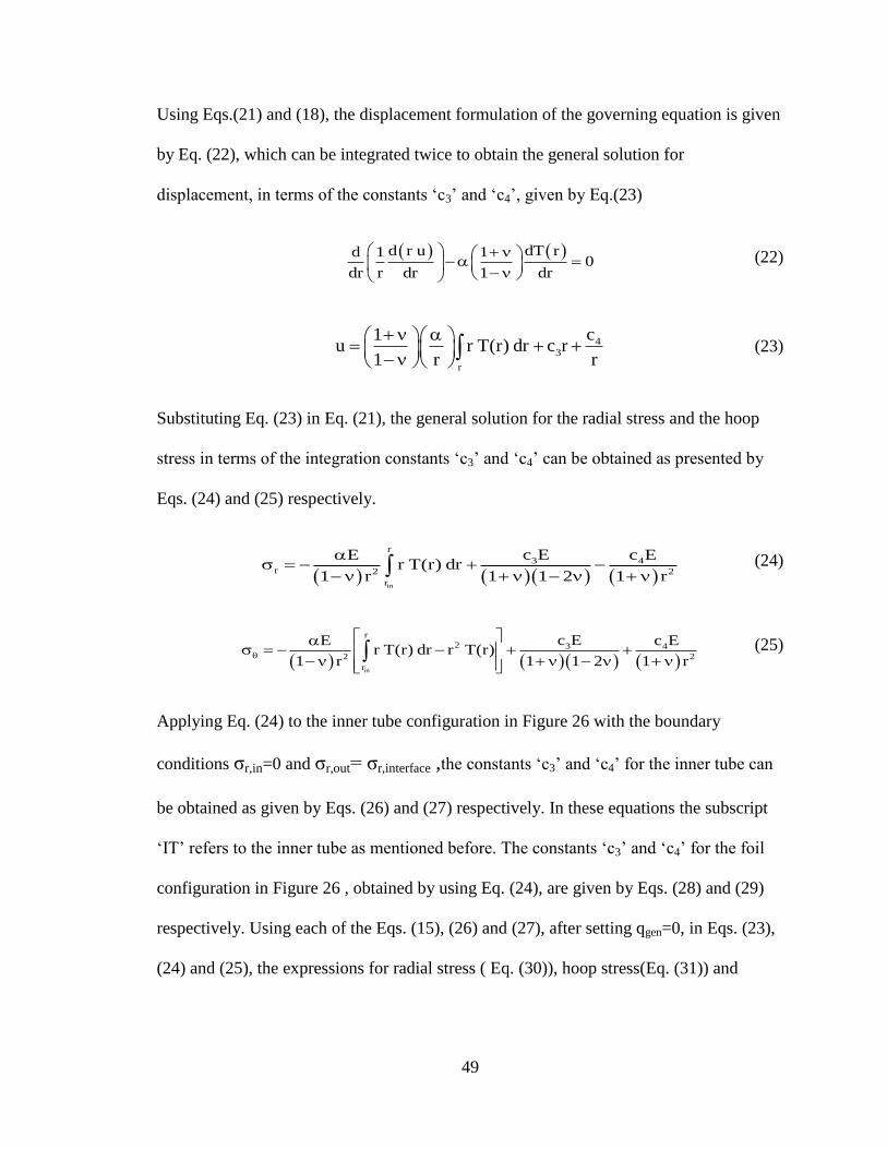
49

Using Eqs.(21) and (18), the displacement formulation of the governing equation is given

by Eq. (22), which can be integrated twice to obtain the general solution for

displacement, in terms of the constants ‘c3’ and ‘c4’, given by Eq.(23)

d r u dT rd 1 10

dr r dr 1 dr

(22)

43

r

c1u r T(r) dr c r

1 r r

(23)

Substituting Eq. (23) in Eq. (21), the general solution for the radial stress and the hoop

stress in terms of the integration constants ‘c3’ and ‘c4’ can be obtained as presented by

Eqs. (24) and (25) respectively.

in

r

3 4r 2 2

r

c E c EEr T(r) dr

1 r 1 1 2 1 r

(24)

in

r

2 3 4

2 2

r

c E c EEr T(r) dr r T(r)

1 r 1 1 2 1 r

(25)

Applying Eq. (24) to the inner tube configuration in Figure 26 with the boundary

conditions σr,in=0 and σr,out= σr,interface ,the constants ‘c3’ and ‘c4’ for the inner tube can

be obtained as given by Eqs. (26) and (27) respectively. In these equations the subscript

‘IT’ refers to the inner tube as mentioned before. The constants ‘c3’ and ‘c4’ for the foil

configuration in Figure 26 , obtained by using Eq. (24), are given by Eqs. (28) and (29)

respectively. Using each of the Eqs. (15), (26) and (27), after setting qgen=0, in Eqs. (23),

(24) and (25), the expressions for radial stress ( Eq. (30)), hoop stress(Eq. (31)) and

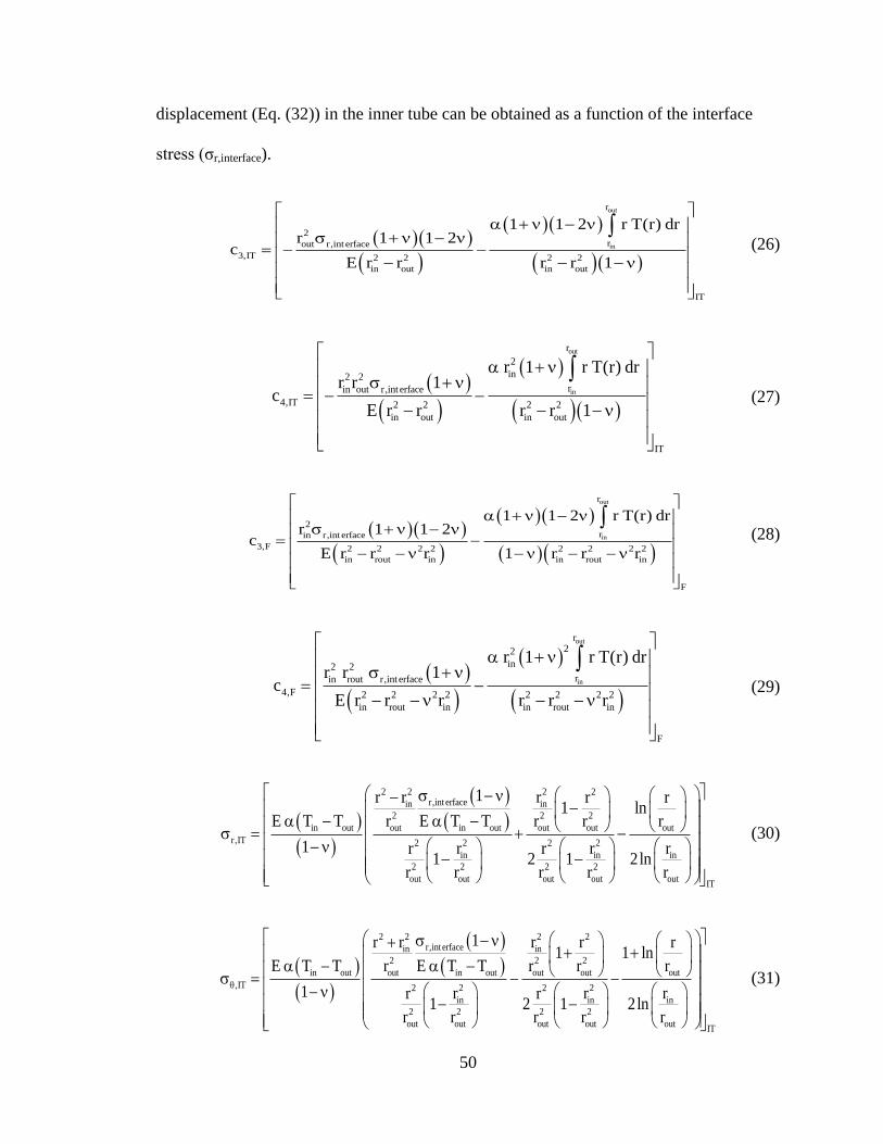
50

displacement (Eq. (32)) in the inner tube can be obtained as a function of the interface

stress (σr,interface).

out

in

r

2rout r,int erface

3,IT 2 2 2 2

in out in out

IT

1 1 2 r T(r) drr 1 1 2

cE r r r r 1

(26)

out

in

r

2

in2 2rin out r,int erface

4,IT 2 2 2 2

in out in out

IT

r 1 r T(r) drr r 1

cE r r r r 1

(27)

out

in

r

2rin r,int erface

3,F 2 2 2 2 2 2 2 2

in rout in in rout in

F

1 1 2 r T(r) drr 1 1 2

cE r r r 1 r r r

(28)

out

in

r22

in2 2rin rout r,int erface

4,F 2 2 2 2 2 2 2 2

in rout in in rout in

F

r 1 r T(r) drr r 1

cE r r r r r r

(29)

22 2 2r,int erface inin

2 22

out out outin out out in out

r,IT 2 22 2

in in in

2 2 2 2

out out out out outIT

1 rr r r r1 ln

r r rE T T r E T T

1 r r rr r1 2 1 2ln

r r r r r

(30)

22 2 2r,int erface inin

2 22

out out outin out out in out

,IT 2 22 2

in in in

2 2 2 2

out out out out outIT

1 rr r r r1 1 ln

r r rE T T r E T T

1 r r rr r1 2 1 2ln

r r r r r

(31)

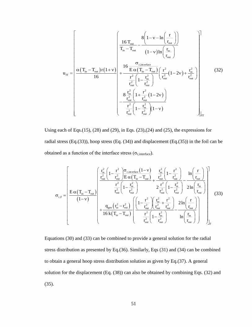
51

outout

in out in

out

r,int erface

22in out in out in

IT 2 222out outin

2 2

out out

2 2

in

2 2

out out

22

in

2 2

out out

r8 1 ln

r16 T

T T r1 ln

r

16T T r 1 E T T rr

u 1 216 r rrr

1r r

r r8 1 1 2

r r

rr1

r r

IT

1

(32)

Using each of Eqs.(15), (28) and (29), in Eqs. (23),(24) and (25), the expressions for

radial stress (Eq.(33)), hoop stress (Eq. (34)) and displacement (Eq.(35)) in the foil can be

obtained as a function of the interface stress (σr,interface).

2 22 2r,int erfacein in

2 2 2 2

out out in out out out out

2 22 2

in in in

2 2 2 2

out out out out outin out

r,F

2 2

gen in out

in out

1r rr r r1 1 ln

r r E T T r r r

r r rr r1 2 1 2ln

r r r r rE T T

1 r1

q r r

16 k T T

22 2

in

2 2 2

out out out out

22

in in

2 2

out out outF

r r r2 ln

r r r r

r rr1 ln

r r r

(33)

Equations (30) and (33) can be combined to provide a general solution for the radial

stress distribution as presented by Eq.(36). Similarly, Eqs (31) and (34) can be combined

to obtain a general hoop stress distribution solution as given by Eq.(37). A general

solution for the displacement (Eq. (38)) can also be obtained by combining Eqs. (32) and

(35).

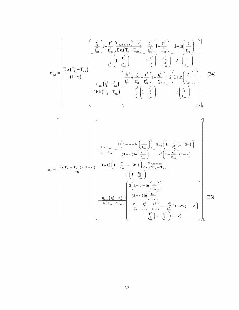
52


2 2 2 2

out out in out out out out

2 22 2

in in in

2 2 2 2

out out out out out

in out

,F

2 2

gen in out

in out

1r rr r r1 1 1 ln

r r E T T r r r

r r rr r1 2 1 2ln

r r r r rE T T

1

q r r

16 k T T

2 24 2

in in

4 2 2 2outout out out out

22

in in

2 2

out out out

F

rr r3r r2 1 ln1

rr r r r

r rr1 ln

r r r

(34)

22

in 2out outout

22in out in in

2

out out

2r,int erface2

in 2

out in outin out

F 22 in

2

out

2

gen in

r r8 1 ln 8 r 1 1 2

r r16 T

T T r r1 ln r 1 1

r r

r16 r 1 1 2

r E T TT T r 1u

16 rr 1

r

q r r

in

in2

out out

2 24 2in out

in in

4 2 2 2

out out out out

22

in

2 2

out out

r2 1 ln

r

r1 ln

r

k T T r rr r3 1 2 2

r r r r

rr1 1

r r

F

(35)

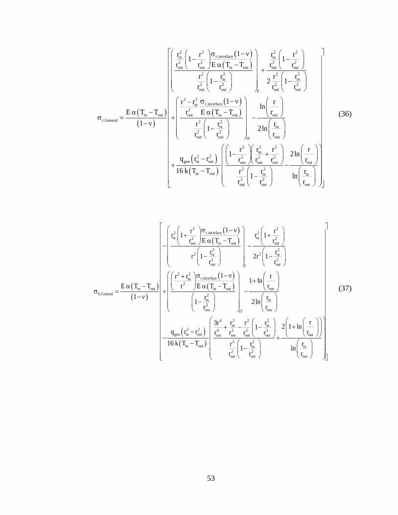
53


2 2 2 2

out out in out out out

2 22 2

in in

2 2 2 2

out out out outF

2 2r,int erfacein

2

in out out in out

r,General

1r rr r1 1

r r E T T r r

r rr r1 2 1

r r r r

1r r

E T T r E T T

1

out

22

in in

2 2

out out outIT

22 2

in2 2 2 2 2

gen in out out out out out

22in out in in

2 2

out out out

rln

r

r rr1 2ln

r r r

rr r r1 2ln

q r r r r r r

16 k T T r rr1 ln

r r r

(36)

2 2r,int erface2 2

in in2 2

out in out out

2 22 2in in

2 2

out outF

2 2r,int erfacein

2

in out in out

,General 2

in

2

out

1r rr 1 r 1

r E T T r

r rr 1 2r 1

r r

1r r

E T T r E T T

1 r1

r

out

in

outIT

2 24 2

in in2 2 4 2 2 2

gen in out outout out out out

22in out in in

2 2

out out out

r1 ln

r

r2 ln

r

rr r3r r2 1 ln1

q r r rr r r r

16 k T T r rr1 ln

r r r

(37)

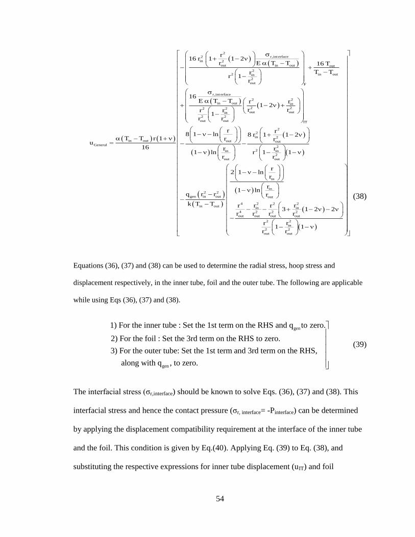
54

2r,int erface2

in 2

out in out out

22 in outin

2

out F

r,int erface

22in out in

2 222out outin

2 2

out out

in out

General

r16 r 1 1 2

r E T T 16 T

T Trr 1

r

16E T T rr

1 2r rrr

1r r

T T r 1u

16

IT

22

in 2out out

22in in

2

out out

in

in2 2

gen in out out

2 24 2in out

in in

4 2 2

out out out

r r8 1 ln 8 r 1 1 2

r r

r r1 ln r 1 1

r r

r2 1 ln

r

r1 ln

q r r r

k T T r rr r3

r r r

2

out

22

in

2 2

out out

1 2 2r

rr1 1

r r

(38)

Equations (36), (37) and (38) can be used to determine the radial stress, hoop stress and

displacement respectively, in the inner tube, foil and the outer tube. The following are applicable

while using Eqs (36), (37) and (38).

gen1) For the inner tube : Set the 1st term on the RHS and q to zero.

2) For the foil : Set the 3rd term on the RHS to zero.

3) For the outer tube: Set the 1st term and 3rd term on the RHS,

along wit genh q , to zero.

(39)

The interfacial stress (σr,interface) should be known to solve Eqs. (36), (37) and (38). This

interfacial stress and hence the contact pressure (σr, interface= -Pinterface) can be determined

by applying the displacement compatibility requirement at the interface of the inner tube

and the foil. This condition is given by Eq.(40). Applying Eq. (39) to Eq. (38), and

substituting the respective expressions for inner tube displacement (uIT) and foil

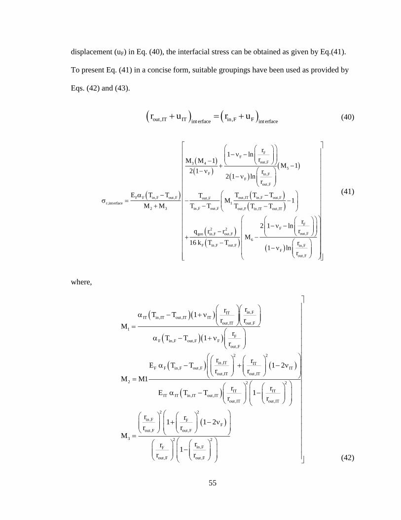
55

displacement (uF) in Eq. (40), the interfacial stress can be obtained as given by Eq.(41).

To present Eq. (41) in a concise form, suitable groupings have been used as provided by

Eqs. (42) and (43).

out,IT IT in,F Fint erface int erfacer u r u (40)

FF

out,F3 4

5

F in,F

F

out,F

F F in,F out,F out,IT in,F out,Fout,F

r,int erface 1

2 3 in,F out,F out,F in,IT out,IT

2 2

gen in,F out,F

F

r1 ln

rM M 1M 1

2 1 r2 1 ln

r

E T T T T TTM 1

M M T T T T T

q r r

16 k

FF

out,F

6

in,F out,F in,F

F

out,F

r2 1 ln

rM

T T r1 ln

r

(41)

where,

in,FITIT in,IT out,IT IT

out,IT out,F

1

FF in,F out,F F

out,F

2 2

in,IT ITF F in,F out,F IT

out,IT out,IT

2

ITIT IT in,IT out,IT

out

rrT T 1

r rM

rT T 1

r

r rE T T 1 2

r rM M1

rE T T

r

2 2

IT

,IT out,IT

2 2

in,F FF

out,F out,F

3 2 2

in,FF

out,F out,F

r1

r

r r1 1 2

r rM

rr1

r r

(42)

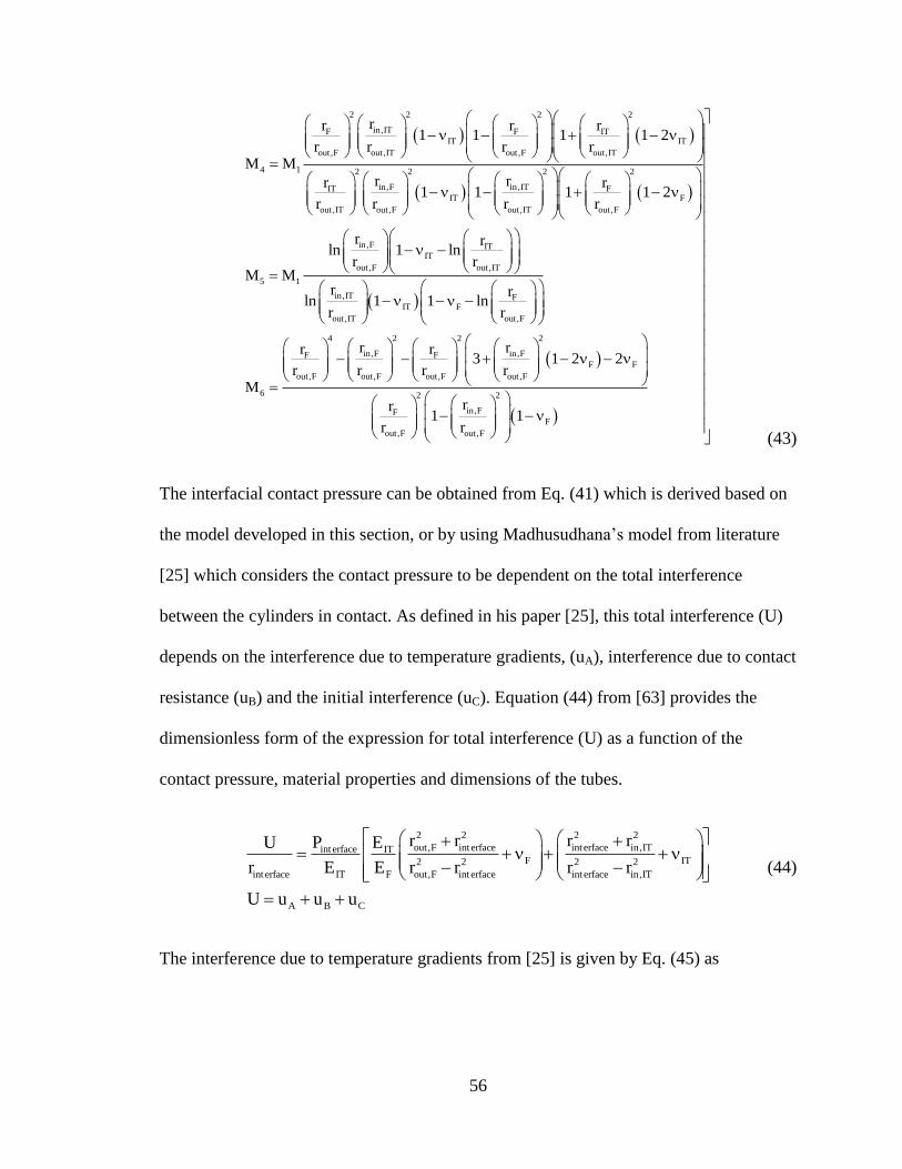
56

2 2 2 2

in,ITF F ITIT IT

out,F out,IT out,F out,IT

4 1 2 2 2

in,F in,ITIT FIT

out,IT out,F out,IT out,F

rr r r1 1 1 1 2

r r r rM M

r rr r1 1 1

r r r r

2

F

in,F ITIT

out,F out,IT

5 1

in,IT FIT F

out,IT out,F

4 2 2

in,FF F

out,F out,F out,F

6

1 2

r rln 1 ln

r rM M

r rln 1 1 ln

r r

r rr r3

r r rM

2

in,F

F F

out,F

2 2

in,FFF

out,F out,F

1 2 2r

rr1 1

r r

(43)

The interfacial contact pressure can be obtained from Eq. (41) which is derived based on

the model developed in this section, or by using Madhusudhana’s model from literature

[25] which considers the contact pressure to be dependent on the total interference

between the cylinders in contact. As defined in his paper [25], this total interference (U)

depends on the interference due to temperature gradients, (uA), interference due to contact

resistance (uB) and the initial interference (uC). Equation (44) from [63] provides the

dimensionless form of the expression for total interference (U) as a function of the

contact pressure, material properties and dimensions of the tubes.

2 2 2 2

out,F int erface int erface in,ITint erface ITF IT2 2 2 2

int erface IT F out,F int erface int erface in,IT

A B C

r r r rP EU

r E E r r r r

U u u u

(44)

The interference due to temperature gradients from [25] is given by Eq. (45) as

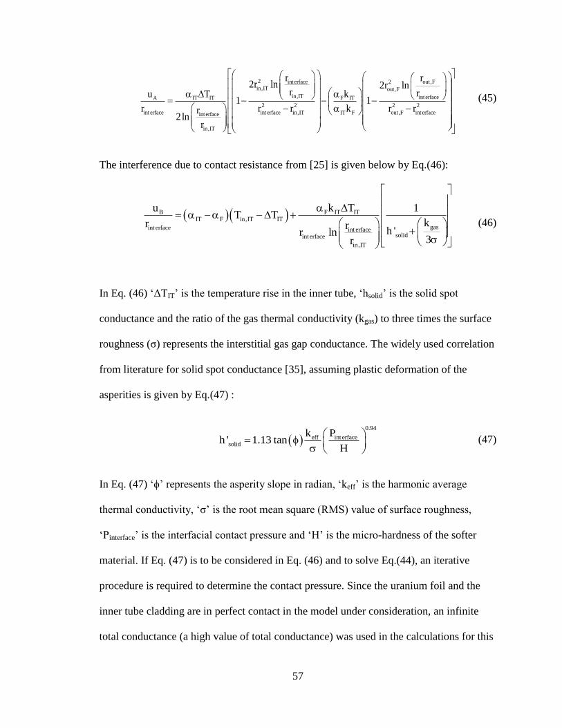
57

2 int erface out,F2in,IT out,F

in,IT int erfaceA IT IT F IT

2 2 2 2

int erface int erface in,IT IT F out,F int erfaceint erface

in,IT

r r2r ln 2r ln

r ru T k1 1

r r r k r rr2ln

r

(45)

The interference due to contact resistance from [25] is given below by Eq.(46):

B F IT IT

IT F in,IT IT

gasint erface int erfacesolidint erface

in,IT

u k T 1T T

kr rh 'r ln

3r

(46)

In Eq. (46) ‘ΔTIT’ is the temperature rise in the inner tube, ‘hsolid’ is the solid spot

conductance and the ratio of the gas thermal conductivity (kgas) to three times the surface

roughness (σ) represents the interstitial gas gap conductance. The widely used correlation

from literature for solid spot conductance [35], assuming plastic deformation of the

asperities is given by Eq.(47) :

0.94

eff int erfacesolid

k Ph ' 1.13 tan

H

(47)

In Eq. (47) ‘ϕ’ represents the asperity slope in radian, ‘keff’ is the harmonic average

thermal conductivity, ‘σ’ is the root mean square (RMS) value of surface roughness,

‘Pinterface’ is the interfacial contact pressure and ‘H’ is the micro-hardness of the softer

material. If Eq. (47) is to be considered in Eq. (46) and to solve Eq.(44), an iterative

procedure is required to determine the contact pressure. Since the uranium foil and the

inner tube cladding are in perfect contact in the model under consideration, an infinite

total conductance (a high value of total conductance) was used in the calculations for this

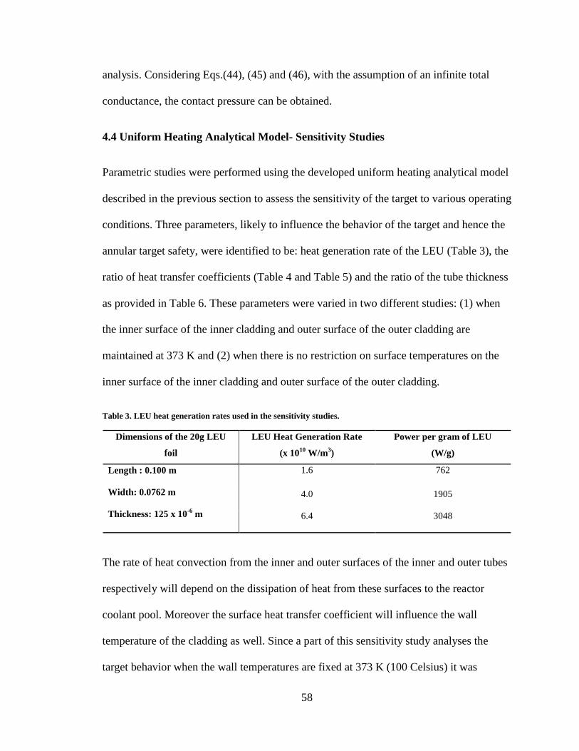
58

analysis. Considering Eqs.(44), (45) and (46), with the assumption of an infinite total

conductance, the contact pressure can be obtained.

4.4 Uniform Heating Analytical Model- Sensitivity Studies

Parametric studies were performed using the developed uniform heating analytical model

described in the previous section to assess the sensitivity of the target to various operating

conditions. Three parameters, likely to influence the behavior of the target and hence the

annular target safety, were identified to be: heat generation rate of the LEU (Table 3), the

ratio of heat transfer coefficients (Table 4 and Table 5) and the ratio of the tube thickness

as provided in Table 6. These parameters were varied in two different studies: (1) when

the inner surface of the inner cladding and outer surface of the outer cladding are

maintained at 373 K and (2) when there is no restriction on surface temperatures on the

inner surface of the inner cladding and outer surface of the outer cladding.

Table 3. LEU heat generation rates used in the sensitivity studies.

Dimensions of the 20g LEU

foil

LEU Heat Generation Rate

(x 1010

W/m3)

Power per gram of LEU

(W/g)

Length : 0.100 m

Width: 0.0762 m

Thickness: 125 x 10-6

m

1.6 762

4.0 1905

6.4 3048

The rate of heat convection from the inner and outer surfaces of the inner and outer tubes

respectively will depend on the dissipation of heat from these surfaces to the reactor

coolant pool. Moreover the surface heat transfer coefficient will influence the wall

temperature of the cladding as well. Since a part of this sensitivity study analyses the

target behavior when the wall temperatures are fixed at 373 K (100 Celsius) it was

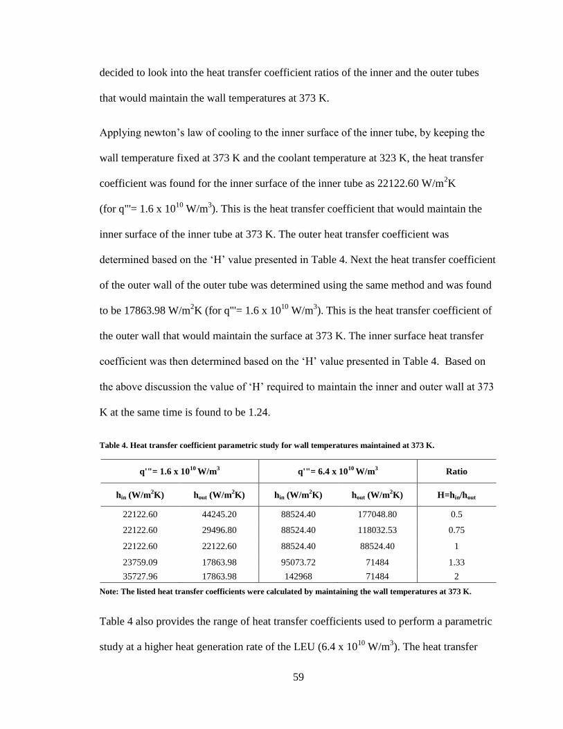
59

decided to look into the heat transfer coefficient ratios of the inner and the outer tubes

that would maintain the wall temperatures at 373 K.

Applying newton’s law of cooling to the inner surface of the inner tube, by keeping the

wall temperature fixed at 373 K and the coolant temperature at 323 K, the heat transfer

coefficient was found for the inner surface of the inner tube as 22122.60 W/m2K

(for q"'= 1.6 x 1010

W/m3). This is the heat transfer coefficient that would maintain the

inner surface of the inner tube at 373 K. The outer heat transfer coefficient was

determined based on the ‘H’ value presented in Table 4. Next the heat transfer coefficient

of the outer wall of the outer tube was determined using the same method and was found

to be 17863.98 W/m2K (for q"'= 1.6 x 10

10 W/m

3). This is the heat transfer coefficient of

the outer wall that would maintain the surface at 373 K. The inner surface heat transfer

coefficient was then determined based on the ‘H’ value presented in Table 4. Based on

the above discussion the value of ‘H’ required to maintain the inner and outer wall at 373

K at the same time is found to be 1.24.

Table 4. Heat transfer coefficient parametric study for wall temperatures maintained at 373 K.

q'"= 1.6 x 1010

W/m3 q'"= 6.4 x 10

10 W/m

3 Ratio

hin (W/m2K) hout (W/m

2K) hin (W/m

2K) hout (W/m

2K) H=hin/hout

22122.60 44245.20 88524.40 177048.80 0.5

22122.60 29496.80 88524.40 118032.53 0.75

22122.60 22122.60 88524.40 88524.40 1

23759.09 17863.98 95073.72 71484 1.33

35727.96 17863.98 142968 71484 2

Note: The listed heat transfer coefficients were calculated by maintaining the wall temperatures at 373 K.

Table 4 also provides the range of heat transfer coefficients used to perform a parametric

study at a higher heat generation rate of the LEU (6.4 x 1010

W/m3). The heat transfer

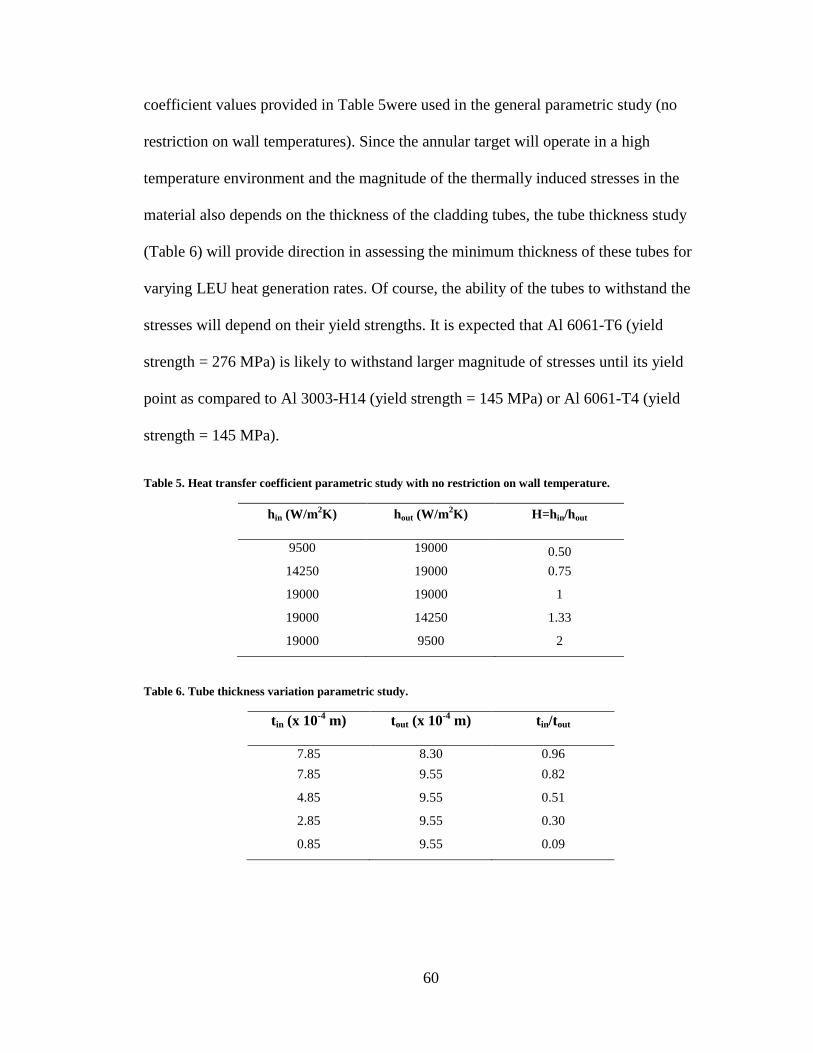
60

coefficient values provided in Table 5were used in the general parametric study (no

restriction on wall temperatures). Since the annular target will operate in a high

temperature environment and the magnitude of the thermally induced stresses in the

material also depends on the thickness of the cladding tubes, the tube thickness study

(Table 6) will provide direction in assessing the minimum thickness of these tubes for

varying LEU heat generation rates. Of course, the ability of the tubes to withstand the

stresses will depend on their yield strengths. It is expected that Al 6061-T6 (yield

strength = 276 MPa) is likely to withstand larger magnitude of stresses until its yield

point as compared to Al 3003-H14 (yield strength = 145 MPa) or Al 6061-T4 (yield

strength = 145 MPa).

Table 5. Heat transfer coefficient parametric study with no restriction on wall temperature.

hin (W/m2K) hout (W/m

2K) H=hin/hout

9500 19000 0.50

14250 19000 0.75

19000 19000 1

19000 14250 1.33

19000 9500 2

Table 6. Tube thickness variation parametric study.

tin (x 10-4

m) tout (x 10-4

m) tin/tout

7.85 8.30 0.96

7.85 9.55 0.82

4.85 9.55 0.51

2.85 9.55 0.30

0.85 9.55 0.09

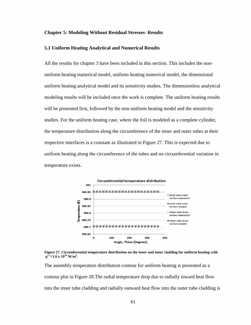
61

Chapter 5: Modeling Without Residual Stresses- Results

5.1 Uniform Heating Analytical and Numerical Results

All the results for chapter 3 have been included in this section. This includes the non-

uniform heating numerical model, uniform heating numerical model, the dimensional

uniform heating analytical model and its sensitivity studies. The dimensionless analytical

modeling results will be included once the work is complete. The uniform heating results

will be presented first, followed by the non-uniform heating model and the sensitivity

studies. For the uniform heating case, where the foil is modeled as a complete cylinder,

the temperature distribution along the circumference of the inner and outer tubes at their

respective interfaces is a constant as illustrated in Figure 27. This is expected due to

uniform heating along the circumference of the tubes and no circumferential variation in

temperature exists.

Figure 27. Circumferential temperature distribution on the inner and outer cladding for uniform heating with

q'''=1.6 x 1010 W/m3.

The assembly temperature distribution contour for uniform heating is presented as a

contour plot in Figure 28.The radial temperature drop due to radially inward heat flow

into the inner tube cladding and radially outward heat flow into the outer tube cladding is

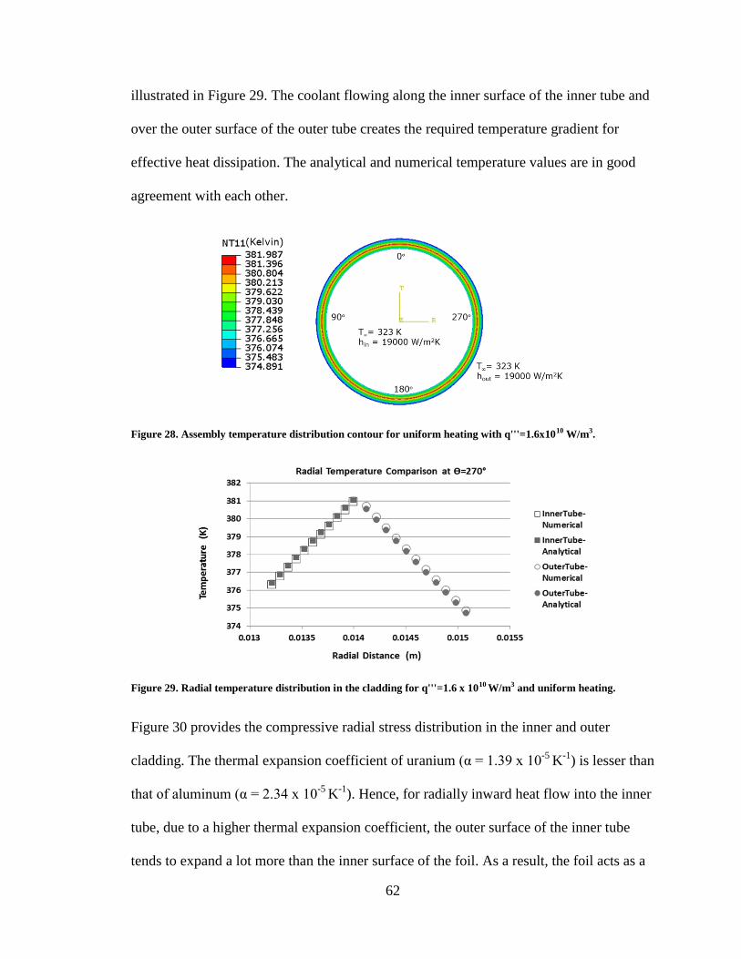
62

illustrated in Figure 29. The coolant flowing along the inner surface of the inner tube and

over the outer surface of the outer tube creates the required temperature gradient for

effective heat dissipation. The analytical and numerical temperature values are in good

agreement with each other.

Figure 28. Assembly temperature distribution contour for uniform heating with q'''=1.6x1010 W/m3.

Figure 29. Radial temperature distribution in the cladding for q'''=1.6 x 1010 W/m3 and uniform heating.

Figure 30 provides the compressive radial stress distribution in the inner and outer

cladding. The thermal expansion coefficient of uranium (α = 1.39 x 10-5

K-1

) is lesser than

that of aluminum (α = 2.34 x 10-5

K-1

). Hence, for radially inward heat flow into the inner

tube, due to a higher thermal expansion coefficient, the outer surface of the inner tube

tends to expand a lot more than the inner surface of the foil. As a result, the foil acts as a

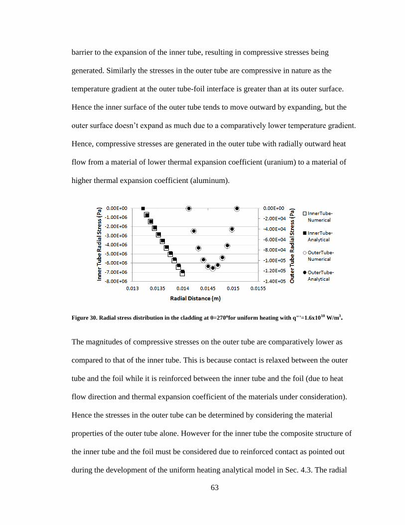
63

barrier to the expansion of the inner tube, resulting in compressive stresses being

generated. Similarly the stresses in the outer tube are compressive in nature as the

temperature gradient at the outer tube-foil interface is greater than at its outer surface.

Hence the inner surface of the outer tube tends to move outward by expanding, but the

outer surface doesn’t expand as much due to a comparatively lower temperature gradient.

Hence, compressive stresses are generated in the outer tube with radially outward heat

flow from a material of lower thermal expansion coefficient (uranium) to a material of

higher thermal expansion coefficient (aluminum).

Figure 30. Radial stress distribution in the cladding at θ=270ᵒfor uniform heating with q"'=1.6x1010 W/m3.

The magnitudes of compressive stresses on the outer tube are comparatively lower as

compared to that of the inner tube. This is because contact is relaxed between the outer

tube and the foil while it is reinforced between the inner tube and the foil (due to heat

flow direction and thermal expansion coefficient of the materials under consideration).

Hence the stresses in the outer tube can be determined by considering the material

properties of the outer tube alone. However for the inner tube the composite structure of

the inner tube and the foil must be considered due to reinforced contact as pointed out

during the development of the uniform heating analytical model in Sec. 4.3. The radial

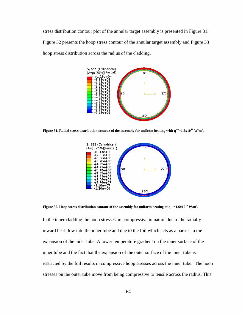
64

stress distribution contour plot of the annular target assembly is presented in Figure 31.

Figure 32 presents the hoop stress contour of the annular target assembly and Figure 33

hoop stress distribution across the radius of the cladding.

Figure 31. Radial stress distribution contour of the assembly for uniform heating with q'''=1.6x1010 W/m3.

Figure 32. Hoop stress distribution contour of the assembly for uniform heating at q'''=1.6x1010 W/m3.

In the inner cladding the hoop stresses are compressive in nature due to the radially

inward heat flow into the inner tube and due to the foil which acts as a barrier to the

expansion of the inner tube. A lower temperature gradient on the inner surface of the

inner tube and the fact that the expansion of the outer surface of the inner tube is

restricted by the foil results in compressive hoop stresses across the inner tube. The hoop

stresses on the outer tube move from being compressive to tensile across the radius. This

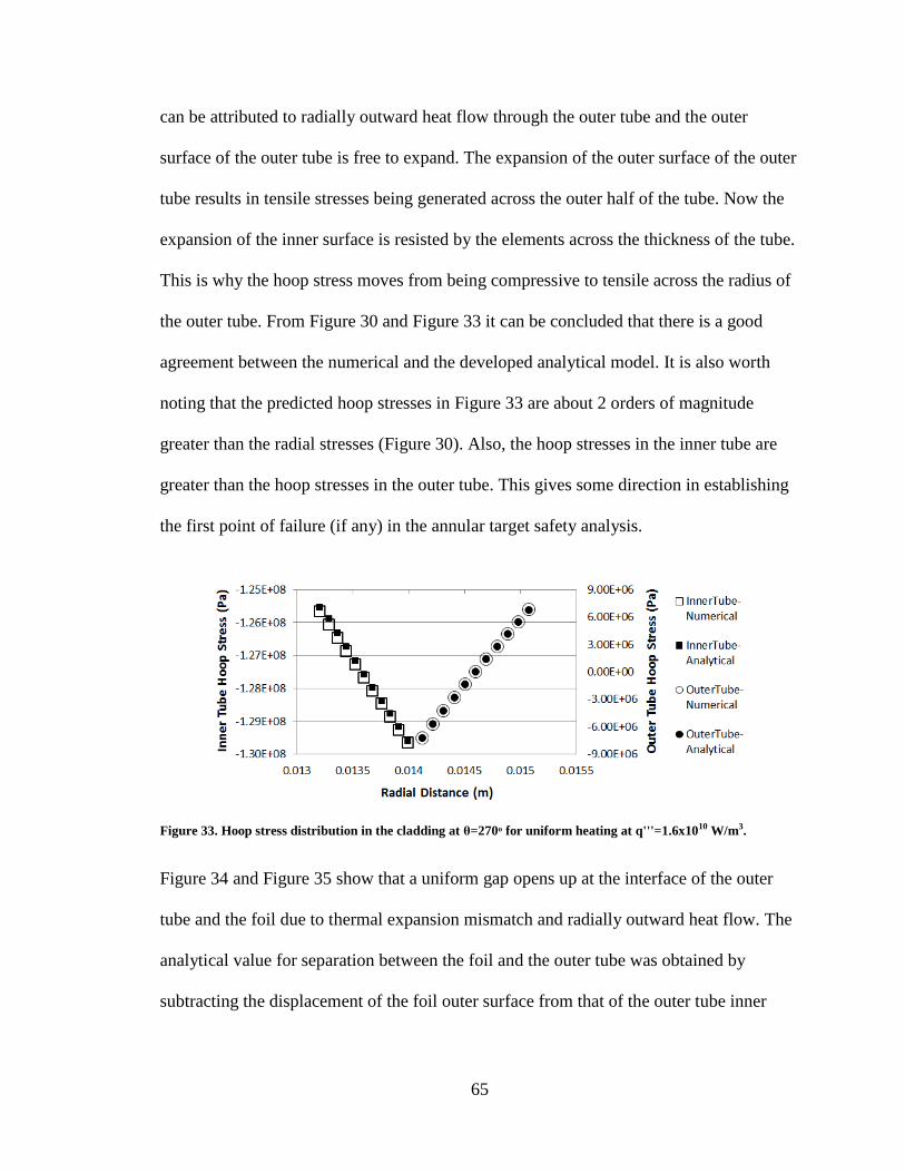
65

can be attributed to radially outward heat flow through the outer tube and the outer

surface of the outer tube is free to expand. The expansion of the outer surface of the outer

tube results in tensile stresses being generated across the outer half of the tube. Now the

expansion of the inner surface is resisted by the elements across the thickness of the tube.

This is why the hoop stress moves from being compressive to tensile across the radius of

the outer tube. From Figure 30 and Figure 33 it can be concluded that there is a good

agreement between the numerical and the developed analytical model. It is also worth

noting that the predicted hoop stresses in Figure 33 are about 2 orders of magnitude

greater than the radial stresses (Figure 30). Also, the hoop stresses in the inner tube are

greater than the hoop stresses in the outer tube. This gives some direction in establishing

the first point of failure (if any) in the annular target safety analysis.

Figure 33. Hoop stress distribution in the cladding at θ=270ᵒ for uniform heating at q'''=1.6x1010 W/m3.

Figure 34 and Figure 35 show that a uniform gap opens up at the interface of the outer

tube and the foil due to thermal expansion mismatch and radially outward heat flow. The

analytical value for separation between the foil and the outer tube was obtained by

subtracting the displacement of the foil outer surface from that of the outer tube inner

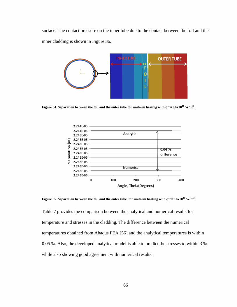
66

surface. The contact pressure on the inner tube due to the contact between the foil and the

inner cladding is shown in Figure 36.

Figure 34. Separation between the foil and the outer tube for uniform heating with q'''=1.6x1010 W/m3.

Figure 35. Separation between the foil and the outer tube for uniform heating with q'''=1.6x1010 W/m3.

Table 7 provides the comparison between the analytical and numerical results for

temperature and stresses in the cladding. The difference between the numerical

temperatures obtained from Abaqus FEA [56] and the analytical temperatures is within

0.05 %. Also, the developed analytical model is able to predict the stresses to within 3 %

while also showing good agreement with numerical results.

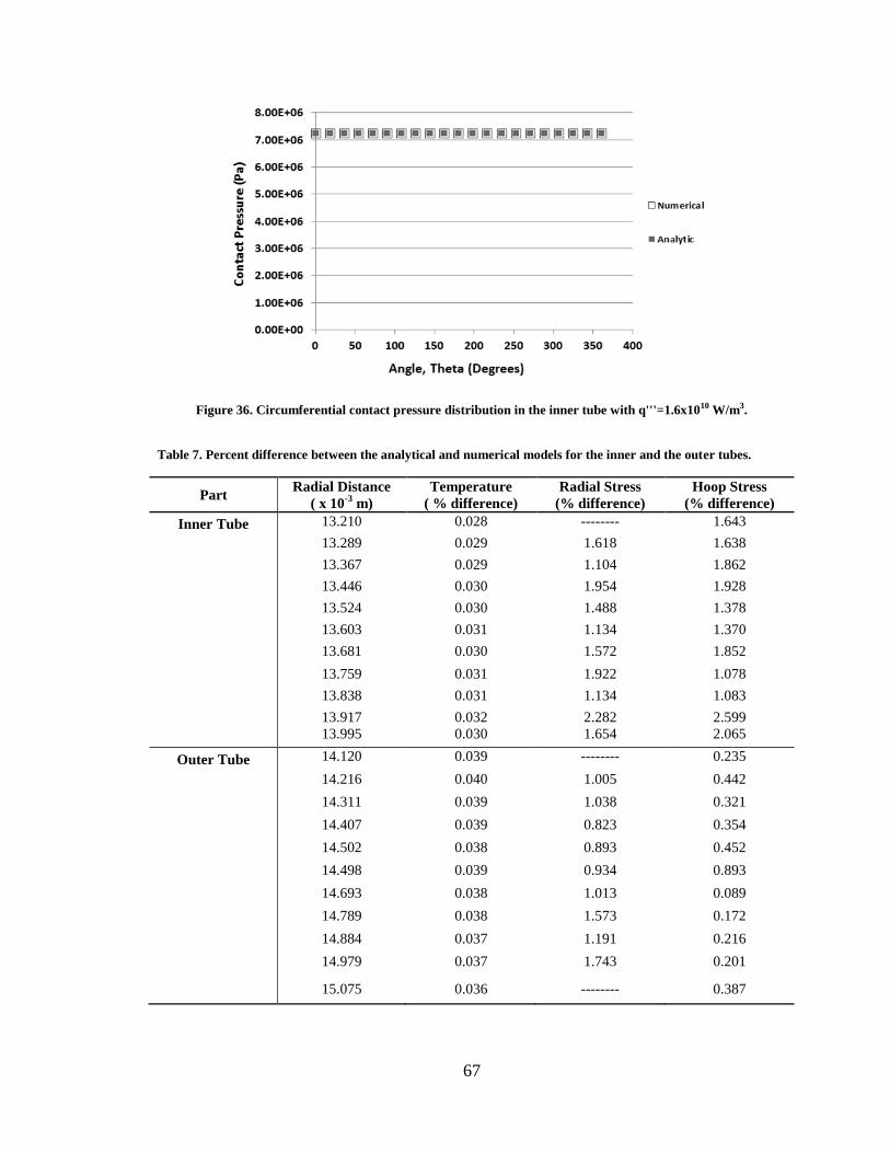
67

Figure 36. Circumferential contact pressure distribution in the inner tube with q'''=1.6x1010 W/m3.

Table 7. Percent difference between the analytical and numerical models for the inner and the outer tubes.

Part Radial Distance

( x 10-3

m)

Temperature

( % difference)

Radial Stress

(% difference)

Hoop Stress

(% difference)

Inner Tube 13.210 0.028 -------- 1.643

13.289 0.029 1.618 1.638

13.367 0.029 1.104 1.862

13.446 0.030 1.954 1.928

13.524 0.030 1.488 1.378

13.603 0.031 1.134 1.370

13.681 0.030 1.572 1.852

13.759 0.031 1.922 1.078

13.838 0.031 1.134 1.083

13.917 0.032 2.282 2.599

13.995 0.030 1.654 2.065

Outer Tube 14.120 0.039 -------- 0.235

14.216 0.040 1.005 0.442

14.311 0.039 1.038 0.321

14.407 0.039 0.823 0.354

14.502 0.038 0.893 0.452

14.498 0.039 0.934 0.893

14.693 0.038 1.013 0.089

14.789 0.038 1.573 0.172

14.884 0.037 1.191 0.216

14.979 0.037 1.743 0.201

15.075 0.036 -------- 0.387

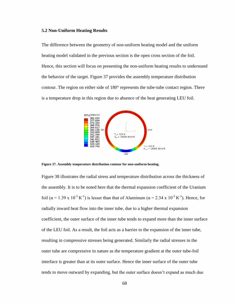
68

5.2 Non-Uniform Heating Results

The difference between the geometry of non-uniform heating model and the uniform

heating model validated in the previous section is the open cross section of the foil.

Hence, this section will focus on presenting the non-uniform heating results to understand

the behavior of the target. Figure 37 provides the assembly temperature distribution

contour. The region on either side of 180° represents the tube-tube contact region. There

is a temperature drop in this region due to absence of the heat generating LEU foil.

Figure 37. Assembly temperature distribution contour for non-uniform heating.

Figure 38 illustrates the radial stress and temperature distribution across the thickness of

the assembly. It is to be noted here that the thermal expansion coefficient of the Uranium

foil (α = 1.39 x 10-5

K-1

) is lesser than that of Aluminum (α = 2.34 x 10-5

K-1

). Hence, for

radially inward heat flow into the inner tube, due to a higher thermal expansion

coefficient, the outer surface of the inner tube tends to expand more than the inner surface

of the LEU foil. As a result, the foil acts as a barrier to the expansion of the inner tube,

resulting in compressive stresses being generated. Similarly the radial stresses in the

outer tube are compressive in nature as the temperature gradient at the outer tube-foil

interface is greater than at its outer surface. Hence the inner surface of the outer tube

tends to move outward by expanding, but the outer surface doesn’t expand as much due

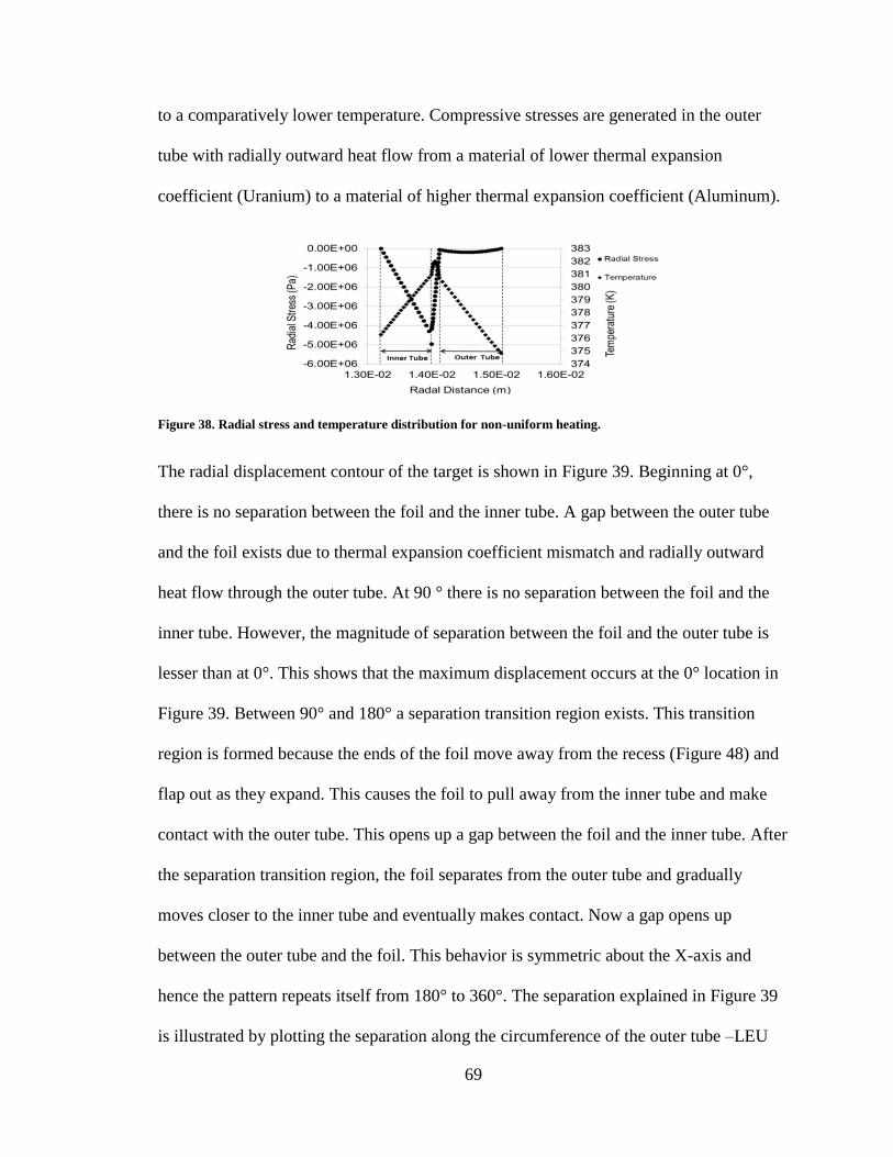
69

to a comparatively lower temperature. Compressive stresses are generated in the outer

tube with radially outward heat flow from a material of lower thermal expansion

coefficient (Uranium) to a material of higher thermal expansion coefficient (Aluminum).

Figure 38. Radial stress and temperature distribution for non-uniform heating.

The radial displacement contour of the target is shown in Figure 39. Beginning at 0°,

there is no separation between the foil and the inner tube. A gap between the outer tube

and the foil exists due to thermal expansion coefficient mismatch and radially outward

heat flow through the outer tube. At 90 ° there is no separation between the foil and the

inner tube. However, the magnitude of separation between the foil and the outer tube is

lesser than at 0°. This shows that the maximum displacement occurs at the 0° location in

Figure 39. Between 90° and 180° a separation transition region exists. This transition

region is formed because the ends of the foil move away from the recess (Figure 48) and

flap out as they expand. This causes the foil to pull away from the inner tube and make

contact with the outer tube. This opens up a gap between the foil and the inner tube. After

the separation transition region, the foil separates from the outer tube and gradually

moves closer to the inner tube and eventually makes contact. Now a gap opens up

between the outer tube and the foil. This behavior is symmetric about the X-axis and

hence the pattern repeats itself from 180° to 360°. The separation explained in Figure 39

is illustrated by plotting the separation along the circumference of the outer tube –LEU

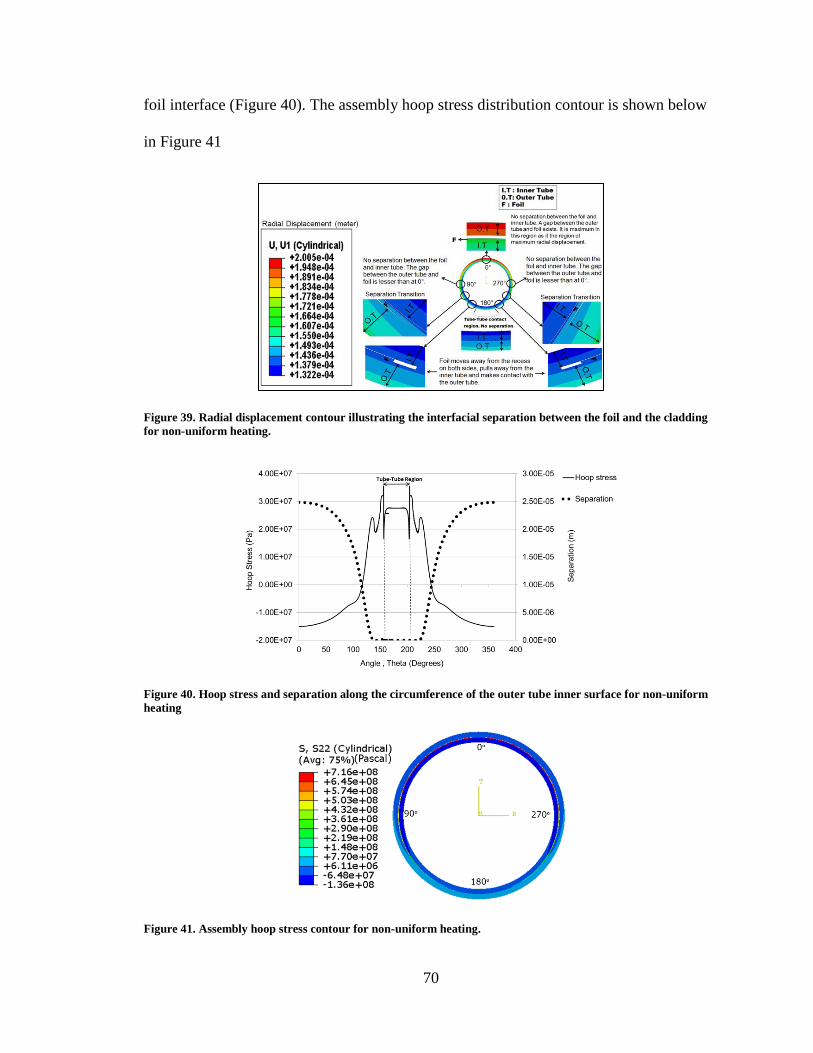
70

foil interface (Figure 40). The assembly hoop stress distribution contour is shown below

in Figure 41

Figure 39. Radial displacement contour illustrating the interfacial separation between the foil and the cladding

for non-uniform heating.

Figure 40. Hoop stress and separation along the circumference of the outer tube inner surface for non-uniform

heating

Figure 41. Assembly hoop stress contour for non-uniform heating.

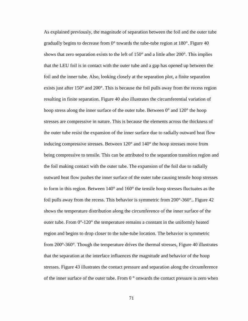
71

As explained previously, the magnitude of separation between the foil and the outer tube

gradually begins to decrease from 0° towards the tube-tube region at 180°. Figure 40

shows that zero separation exists to the left of 150° and a little after 200°. This implies

that the LEU foil is in contact with the outer tube and a gap has opened up between the

foil and the inner tube. Also, looking closely at the separation plot, a finite separation

exists just after 150° and 200°. This is because the foil pulls away from the recess region

resulting in finite separation. Figure 40 also illustrates the circumferential variation of

hoop stress along the inner surface of the outer tube. Between 0° and 120° the hoop

stresses are compressive in nature. This is because the elements across the thickness of

the outer tube resist the expansion of the inner surface due to radially outward heat flow

inducing compressive stresses. Between 120° and 140° the hoop stresses move from

being compressive to tensile. This can be attributed to the separation transition region and

the foil making contact with the outer tube. The expansion of the foil due to radially

outward heat flow pushes the inner surface of the outer tube causing tensile hoop stresses

to form in this region. Between 140° and 160° the tensile hoop stresses fluctuates as the

foil pulls away from the recess. This behavior is symmetric from 200°-360°.. Figure 42

shows the temperature distribution along the circumference of the inner surface of the

outer tube. From 0°-120° the temperature remains a constant in the uniformly heated

region and begins to drop closer to the tube-tube location. The behavior is symmetric

from 200°-360°. Though the temperature drives the thermal stresses, Figure 40 illustrates

that the separation at the interface influences the magnitude and behavior of the hoop

stresses. Figure 43 illustrates the contact pressure and separation along the circumference

of the inner surface of the outer tube. From 0 ° onwards the contact pressure is zero when

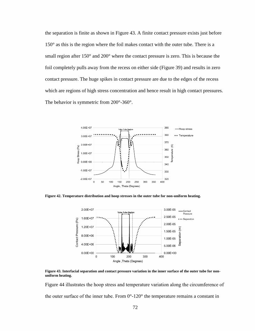
72

the separation is finite as shown in Figure 43. A finite contact pressure exists just before

150° as this is the region where the foil makes contact with the outer tube. There is a

small region after 150° and 200° where the contact pressure is zero. This is because the

foil completely pulls away from the recess on either side (Figure 39) and results in zero

contact pressure. The huge spikes in contact pressure are due to the edges of the recess

which are regions of high stress concentration and hence result in high contact pressures.

The behavior is symmetric from 200°-360°.

Figure 42. Temperature distribution and hoop stresses in the outer tube for non-uniform heating.

Figure 43. Interfacial separation and contact pressure variation in the inner surface of the outer tube for non-

uniform heating.

Figure 44 illustrates the hoop stress and temperature variation along the circumference of

the outer surface of the inner tube. From 0°-120° the temperature remains a constant in

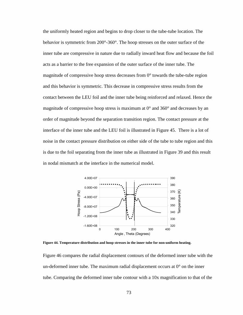
73

the uniformly heated region and begins to drop closer to the tube-tube location. The

behavior is symmetric from 200°-360°. The hoop stresses on the outer surface of the

inner tube are compressive in nature due to radially inward heat flow and because the foil

acts as a barrier to the free expansion of the outer surface of the inner tube. The

magnitude of compressive hoop stress decreases from 0° towards the tube-tube region

and this behavior is symmetric. This decrease in compressive stress results from the

contact between the LEU foil and the inner tube being reinforced and relaxed. Hence the

magnitude of compressive hoop stress is maximum at 0° and 360° and decreases by an

order of magnitude beyond the separation transition region. The contact pressure at the

interface of the inner tube and the LEU foil is illustrated in Figure 45. There is a lot of

noise in the contact pressure distribution on either side of the tube to tube region and this

is due to the foil separating from the inner tube as illustrated in Figure 39 and this result

in nodal mismatch at the interface in the numerical model.

Figure 44. Temperature distribution and hoop stresses in the inner tube for non-uniform heating.

Figure 46 compares the radial displacement contours of the deformed inner tube with the

un-deformed inner tube. The maximum radial displacement occurs at 0° on the inner

tube. Comparing the deformed inner tube contour with a 10x magnification to that of the

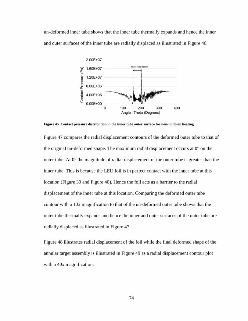
74

un-deformed inner tube shows that the inner tube thermally expands and hence the inner

and outer surfaces of the inner tube are radially displaced as illustrated in Figure 46.

Figure 45. Contact pressure distribution in the inner tube outer surface for non-uniform heating.

Figure 47 compares the radial displacement contours of the deformed outer tube to that of

the original un-deformed shape. The maximum radial displacement occurs at 0° on the

outer tube. At 0° the magnitude of radial displacement of the outer tube is greater than the

inner tube. This is because the LEU foil is in perfect contact with the inner tube at this

location (Figure 39 and Figure 40). Hence the foil acts as a barrier to the radial

displacement of the inner tube at this location. Comparing the deformed outer tube

contour with a 10x magnification to that of the un-deformed outer tube shows that the

outer tube thermally expands and hence the inner and outer surfaces of the outer tube are

radially displaced as illustrated in Figure 47.

Figure 48 illustrates radial displacement of the foil while the final deformed shape of the

annular target assembly is illustrated in Figure 49 as a radial displacement contour plot

with a 40x magnification.

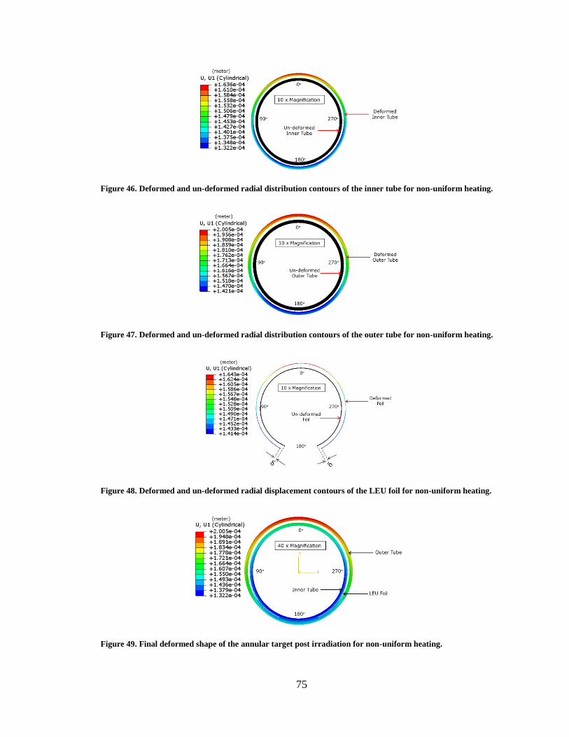
75

Figure 46. Deformed and un-deformed radial distribution contours of the inner tube for non-uniform heating.

Figure 47. Deformed and un-deformed radial distribution contours of the outer tube for non-uniform heating.

Figure 48. Deformed and un-deformed radial displacement contours of the LEU foil for non-uniform heating.

Figure 49. Final deformed shape of the annular target post irradiation for non-uniform heating.

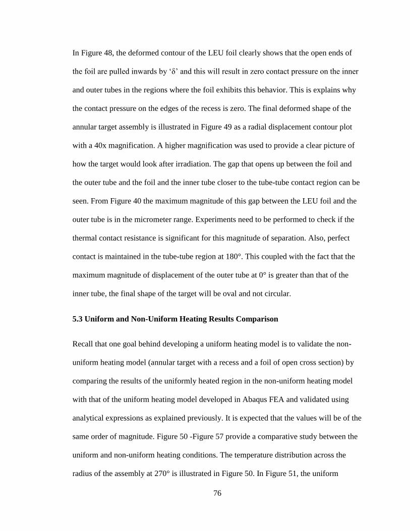
76

In Figure 48, the deformed contour of the LEU foil clearly shows that the open ends of

the foil are pulled inwards by ‘δ’ and this will result in zero contact pressure on the inner

and outer tubes in the regions where the foil exhibits this behavior. This is explains why

the contact pressure on the edges of the recess is zero. The final deformed shape of the

annular target assembly is illustrated in Figure 49 as a radial displacement contour plot

with a 40x magnification. A higher magnification was used to provide a clear picture of

how the target would look after irradiation. The gap that opens up between the foil and

the outer tube and the foil and the inner tube closer to the tube-tube contact region can be

seen. From Figure 40 the maximum magnitude of this gap between the LEU foil and the

outer tube is in the micrometer range. Experiments need to be performed to check if the

thermal contact resistance is significant for this magnitude of separation. Also, perfect

contact is maintained in the tube-tube region at 180°. This coupled with the fact that the

maximum magnitude of displacement of the outer tube at 0° is greater than that of the

inner tube, the final shape of the target will be oval and not circular.

5.3 Uniform and Non-Uniform Heating Results Comparison

Recall that one goal behind developing a uniform heating model is to validate the non-

uniform heating model (annular target with a recess and a foil of open cross section) by

comparing the results of the uniformly heated region in the non-uniform heating model

with that of the uniform heating model developed in Abaqus FEA and validated using

analytical expressions as explained previously. It is expected that the values will be of the

same order of magnitude. Figure 50 -Figure 57 provide a comparative study between the

uniform and non-uniform heating conditions. The temperature distribution across the

radius of the assembly at 270° is illustrated in Figure 50. In Figure 51, the uniform

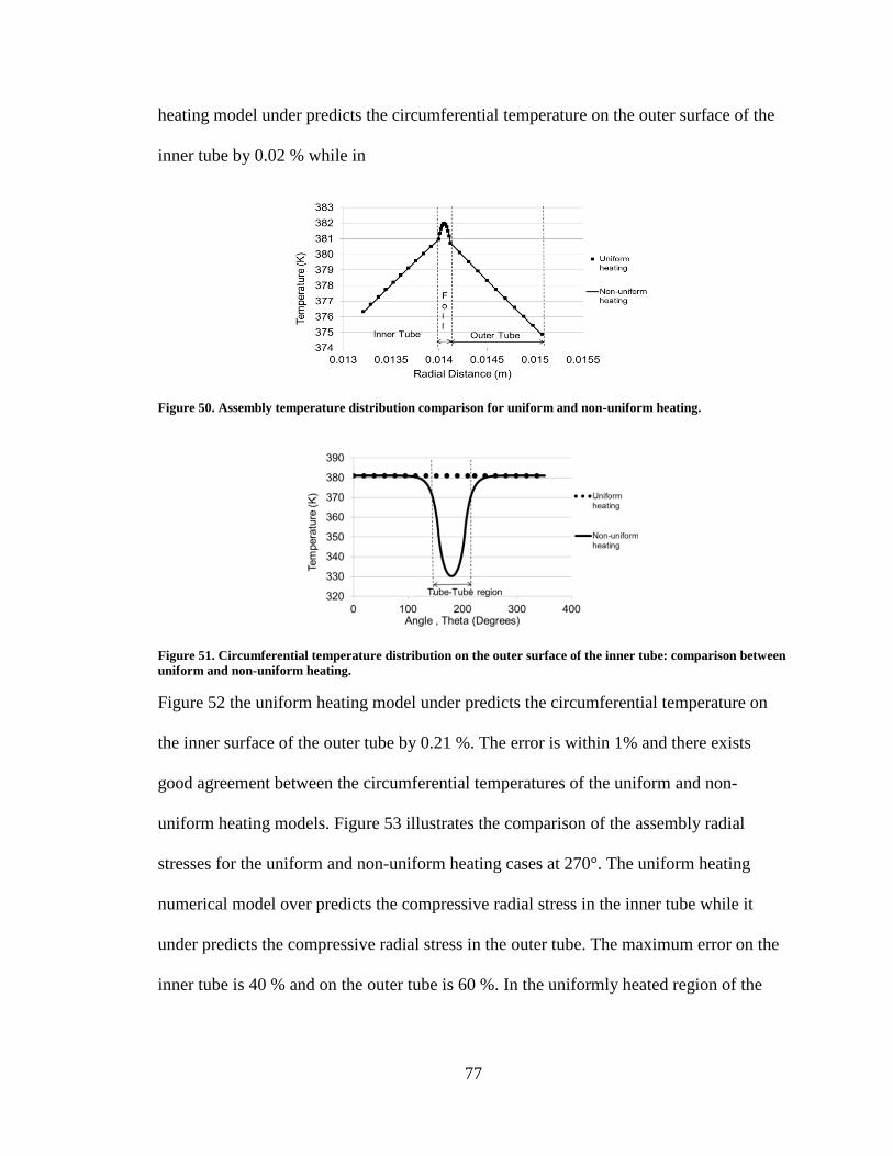
77

heating model under predicts the circumferential temperature on the outer surface of the

inner tube by 0.02 % while in

Figure 50. Assembly temperature distribution comparison for uniform and non-uniform heating.

Figure 51. Circumferential temperature distribution on the outer surface of the inner tube: comparison between

uniform and non-uniform heating.

Figure 52 the uniform heating model under predicts the circumferential temperature on

the inner surface of the outer tube by 0.21 %. The error is within 1% and there exists

good agreement between the circumferential temperatures of the uniform and non-

uniform heating models. Figure 53 illustrates the comparison of the assembly radial

stresses for the uniform and non-uniform heating cases at 270°. The uniform heating

numerical model over predicts the compressive radial stress in the inner tube while it

under predicts the compressive radial stress in the outer tube. The maximum error on the

inner tube is 40 % and on the outer tube is 60 %. In the uniformly heated region of the

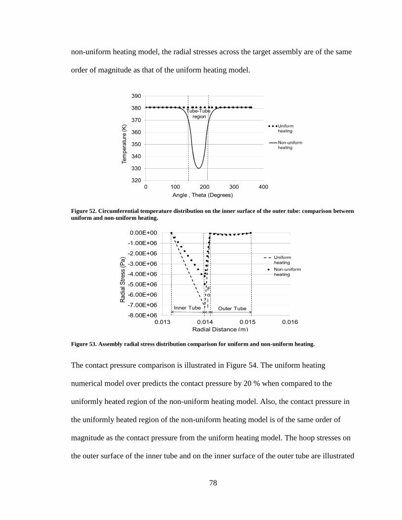
78

non-uniform heating model, the radial stresses across the target assembly are of the same

order of magnitude as that of the uniform heating model.

Figure 52. Circumferential temperature distribution on the inner surface of the outer tube: comparison between

uniform and non-uniform heating.

Figure 53. Assembly radial stress distribution comparison for uniform and non-uniform heating.

The contact pressure comparison is illustrated in Figure 54. The uniform heating

numerical model over predicts the contact pressure by 20 % when compared to the

uniformly heated region of the non-uniform heating model. Also, the contact pressure in

the uniformly heated region of the non-uniform heating model is of the same order of

magnitude as the contact pressure from the uniform heating model. The hoop stresses on

the outer surface of the inner tube and on the inner surface of the outer tube are illustrated

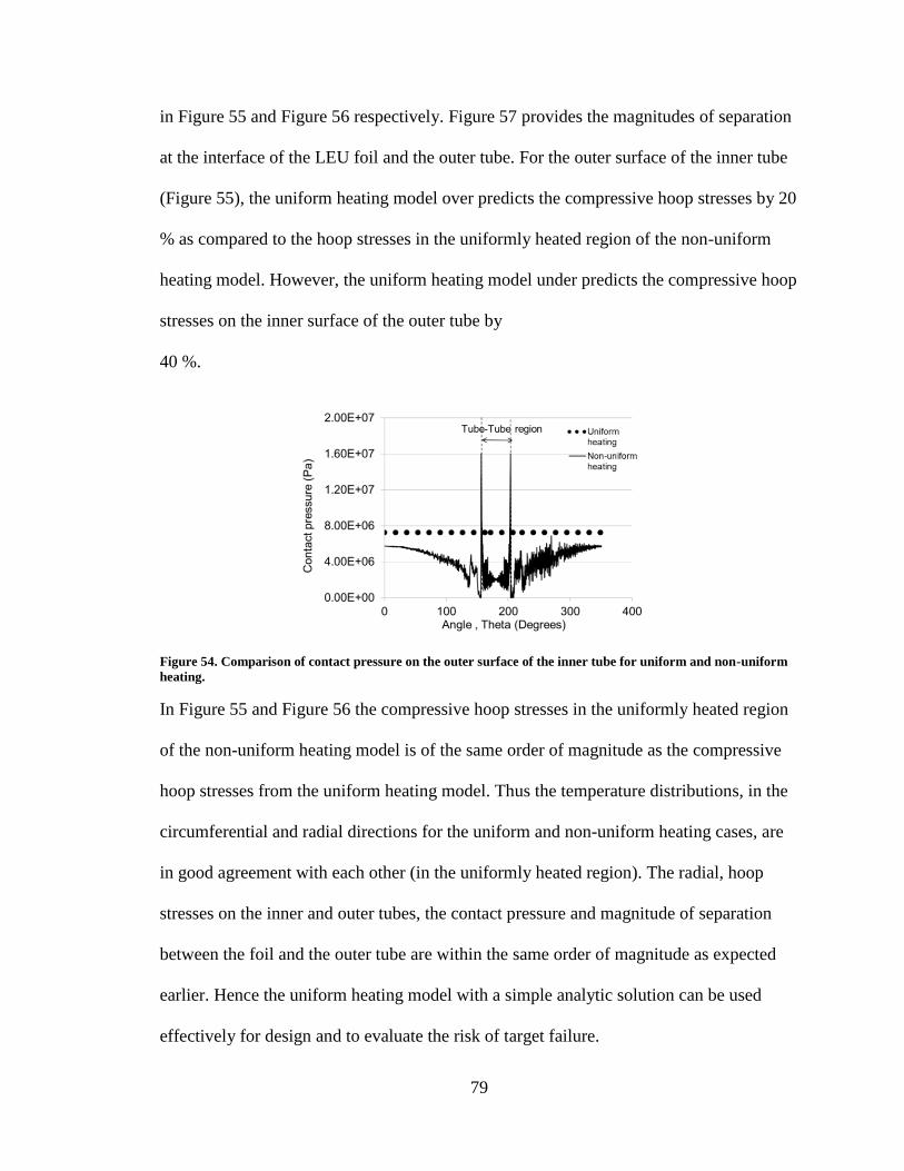
79

in Figure 55 and Figure 56 respectively. Figure 57 provides the magnitudes of separation

at the interface of the LEU foil and the outer tube. For the outer surface of the inner tube

(Figure 55), the uniform heating model over predicts the compressive hoop stresses by 20

% as compared to the hoop stresses in the uniformly heated region of the non-uniform

heating model. However, the uniform heating model under predicts the compressive hoop

stresses on the inner surface of the outer tube by

40 %.

Figure 54. Comparison of contact pressure on the outer surface of the inner tube for uniform and non-uniform

heating.

In Figure 55 and Figure 56 the compressive hoop stresses in the uniformly heated region

of the non-uniform heating model is of the same order of magnitude as the compressive

hoop stresses from the uniform heating model. Thus the temperature distributions, in the

circumferential and radial directions for the uniform and non-uniform heating cases, are

in good agreement with each other (in the uniformly heated region). The radial, hoop

stresses on the inner and outer tubes, the contact pressure and magnitude of separation

between the foil and the outer tube are within the same order of magnitude as expected

earlier. Hence the uniform heating model with a simple analytic solution can be used

effectively for design and to evaluate the risk of target failure.

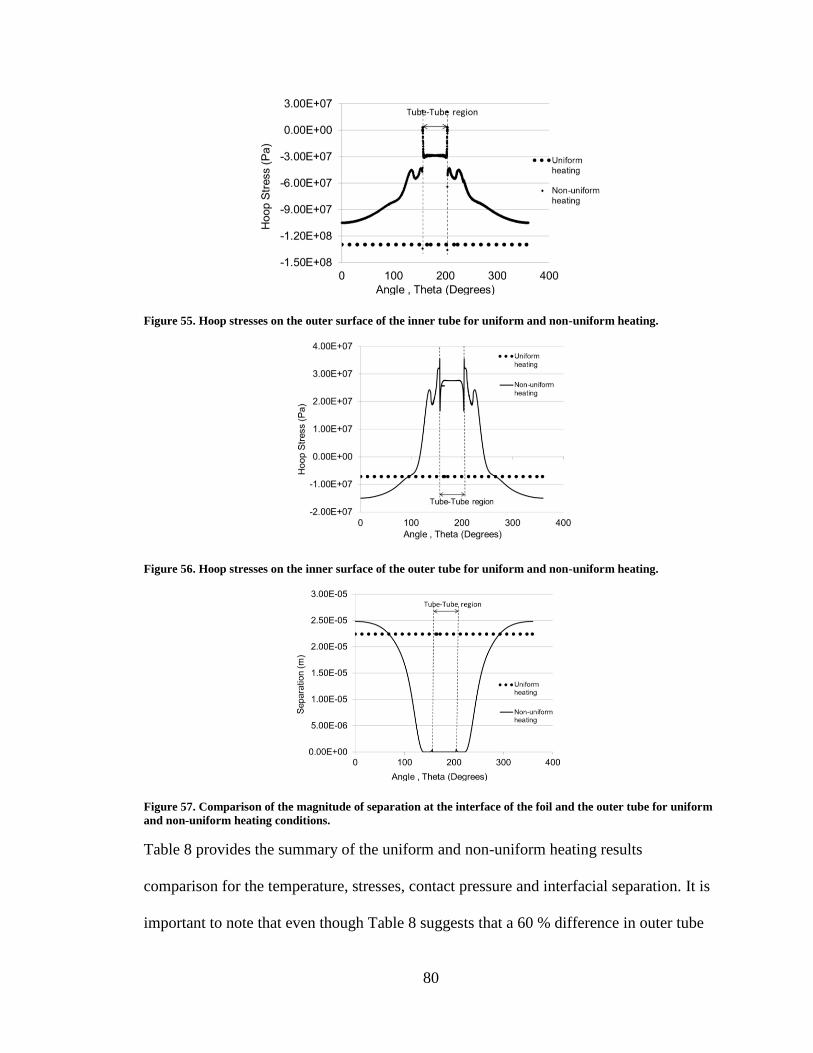
80

Figure 55. Hoop stresses on the outer surface of the inner tube for uniform and non-uniform heating.

Figure 56. Hoop stresses on the inner surface of the outer tube for uniform and non-uniform heating.

Figure 57. Comparison of the magnitude of separation at the interface of the foil and the outer tube for uniform

and non-uniform heating conditions.

Table 8 provides the summary of the uniform and non-uniform heating results

comparison for the temperature, stresses, contact pressure and interfacial separation. It is

important to note that even though Table 8 suggests that a 60 % difference in outer tube

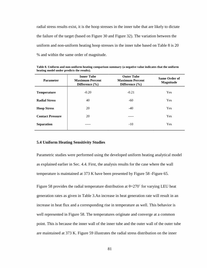
81

radial stress results exist, it is the hoop stresses in the inner tube that are likely to dictate

the failure of the target (based on Figure 30 and Figure 32). The variation between the

uniform and non-uniform heating hoop stresses in the inner tube based on Table 8 is 20

% and within the same order of magnitude.

Table 8. Uniform and non-uniform heating comparison summary (a negative value indicates that the uniform

heating model under predicts the results).

Parameter

Inner Tube

Maximum Percent

Difference (%)

Outer Tube

Maximum Percent

Difference (%)

Same Order of

Magnitude

Temperature

-0.20

-0.21

Yes

Radial Stress 40 -60 Yes

Hoop Stress 20 -40 Yes

Contact Pressure 20 ----- Yes

Separation ----- -10 Yes

5.4 Uniform Heating Sensitivity Studies

Parametric studies were performed using the developed uniform heating analytical model

as explained earlier in Sec. 4.4. First, the analysis results for the case where the wall

temperature is maintained at 373 K have been presented by Figure 58 -Figure 65.

Figure 58 provides the radial temperature distribution at θ=270˚ for varying LEU heat

generation rates as given in Table 3.An increase in heat generation rate will result in an

increase in heat flux and a corresponding rise in temperature as well. This behavior is

well represented in Figure 58. The temperatures originate and converge at a common

point. This is because the inner wall of the inner tube and the outer wall of the outer tube

are maintained at 373 K. Figure 59 illustrates the radial stress distribution on the inner

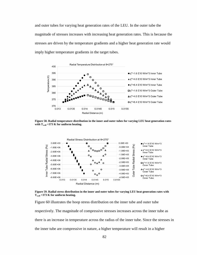
82

and outer tubes for varying heat generation rates of the LEU. In the outer tube the

magnitude of stresses increases with increasing heat generation rates. This is because the

stresses are driven by the temperature gradients and a higher heat generation rate would

imply higher temperature gradients in the target tubes.

Figure 58. Radial temperature distribution in the inner and outer tubes for varying LEU heat generation rates

with Twall =373 K for uniform heating.

Figure 59. Radial stress distribution in the inner and outer tubes for varying LEU heat generation rates with

Twall =373 K for uniform heating.

Figure 60 illustrates the hoop stress distribution on the inner tube and outer tube

respectively. The magnitude of compressive stresses increases across the inner tube as

there is an increase in temperature across the radius of the inner tube. Since the stresses in

the inner tube are compressive in nature, a higher temperature will result in a higher

83

compressive stress state. An increase in the LEU heat generation rate will increase the

magnitude of temperature gradients (Figure 58) and results in a higher compressive

stress.

Figure 60. Hoop stress distribution in the inner and outer tubes for varying LEU heat generation rates with

Twall =373 K for uniform heating.

Figure 60 also shows that the maximum compressive hoop stress is induced on the inner

surface of the outer tube. This is because the inner surface of the outer tube is the surface

closer to the heat generating LEU and the temperature of the outer tube will be the

highest at this point as shown in Figure 58. Next, the inner to outer heat transfer

coefficient ratio was varied based on Table 4 and the results are provided by Figure 61-

Figure 64. Figure 61 shows the variation of temperature at the outer and inner surfaces of

the tubes for various heat transfer coefficient ratios and at the lowest and highest heat

generation rate of the LEU. A heat transfer coefficient ratio of below 1 implies that the

outer surface heat transfer coefficient is greater than that of the inner surface while a heat

transfer coefficient ratio greater than 1 implies a higher inner surface heat transfer

coefficient. In Figure 61, for a heat transfer coefficient ratio of 0.5 the outer surface of the

inner tube is at a higher temperature than the inner surface of the outer tube. This is

because the inner tube inner surface is at a comparatively lower heat transfer coefficient

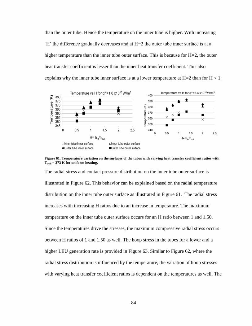
84

than the outer tube. Hence the temperature on the inner tube is higher. With increasing

‘H’ the difference gradually decreases and at H=2 the outer tube inner surface is at a

higher temperature than the inner tube outer surface. This is because for H=2, the outer

heat transfer coefficient is lesser than the inner heat transfer coefficient. This also

explains why the inner tube inner surface is at a lower temperature at H=2 than for H < 1.

Figure 61. Temperature variation on the surfaces of the tubes with varying heat transfer coefficient ratios with

Twall = 373 K for uniform heating.

The radial stress and contact pressure distribution on the inner tube outer surface is

illustrated in Figure 62. This behavior can be explained based on the radial temperature

distribution on the inner tube outer surface as illustrated in Figure 61. The radial stress

increases with increasing H ratios due to an increase in temperature. The maximum

temperature on the inner tube outer surface occurs for an H ratio between 1 and 1.50.

Since the temperatures drive the stresses, the maximum compressive radial stress occurs

between H ratios of 1 and 1.50 as well. The hoop stress in the tubes for a lower and a

higher LEU generation rate is provided in Figure 63. Similar to Figure 62, where the

radial stress distribution is influenced by the temperature, the variation of hoop stresses

with varying heat transfer coefficient ratios is dependent on the temperatures as well. The

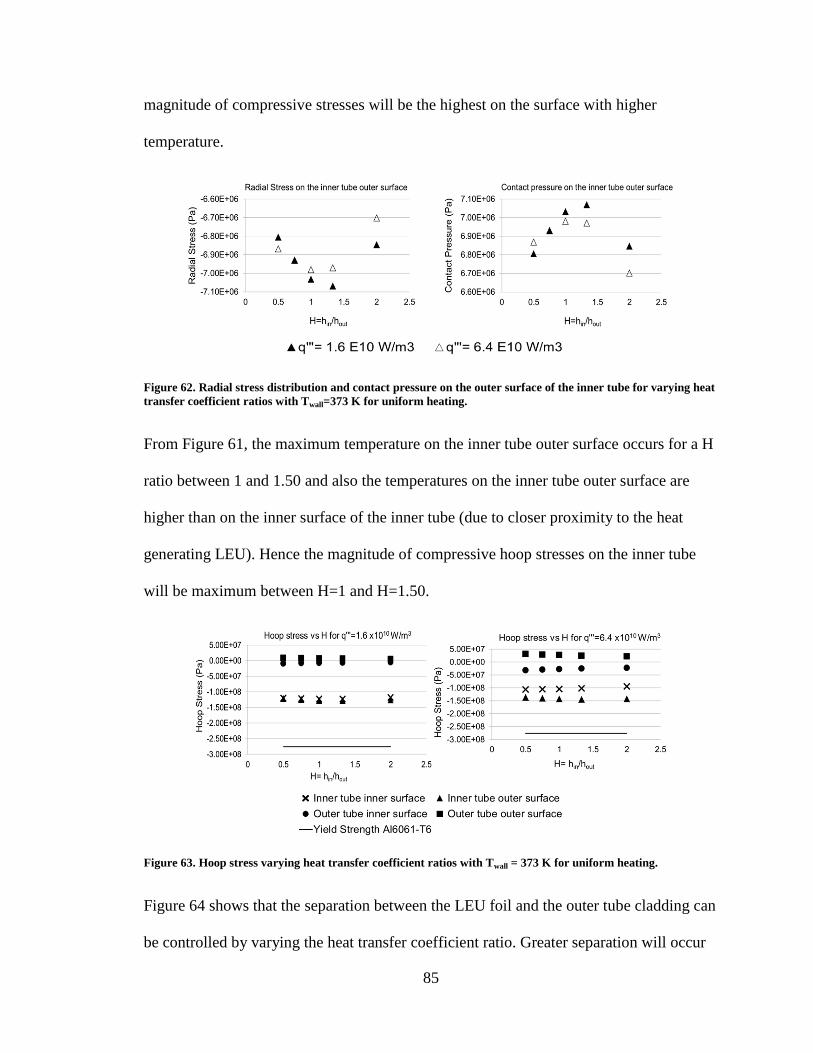
85

magnitude of compressive stresses will be the highest on the surface with higher

temperature.

Figure 62. Radial stress distribution and contact pressure on the outer surface of the inner tube for varying heat

transfer coefficient ratios with Twall=373 K for uniform heating.

From Figure 61, the maximum temperature on the inner tube outer surface occurs for a H

ratio between 1 and 1.50 and also the temperatures on the inner tube outer surface are

higher than on the inner surface of the inner tube (due to closer proximity to the heat

generating LEU). Hence the magnitude of compressive hoop stresses on the inner tube

will be maximum between H=1 and H=1.50.

Figure 63. Hoop stress varying heat transfer coefficient ratios with Twall = 373 K for uniform heating.

Figure 64 shows that the separation between the LEU foil and the outer tube cladding can

be controlled by varying the heat transfer coefficient ratio. Greater separation will occur

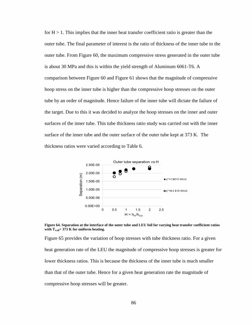
86

for H > 1. This implies that the inner heat transfer coefficient ratio is greater than the

outer tube. The final parameter of interest is the ratio of thickness of the inner tube to the

outer tube. From Figure 60, the maximum compressive stress generated in the outer tube

is about 30 MPa and this is within the yield strength of Aluminum 6061-T6. A

comparison between Figure 60 and Figure 61 shows that the magnitude of compressive

hoop stress on the inner tube is higher than the compressive hoop stresses on the outer

tube by an order of magnitude. Hence failure of the inner tube will dictate the failure of

the target. Due to this it was decided to analyze the hoop stresses on the inner and outer

surfaces of the inner tube. This tube thickness ratio study was carried out with the inner

surface of the inner tube and the outer surface of the outer tube kept at 373 K. The

thickness ratios were varied according to Table 6.

Figure 64. Separation at the interface of the outer tube and LEU foil for varying heat transfer coefficient ratios

with Twall= 373 K for uniform heating.

Figure 65 provides the variation of hoop stresses with tube thickness ratio. For a given

heat generation rate of the LEU the magnitude of compressive hoop stresses is greater for

lower thickness ratios. This is because the thickness of the inner tube is much smaller

than that of the outer tube. Hence for a given heat generation rate the magnitude of

compressive hoop stresses will be greater.

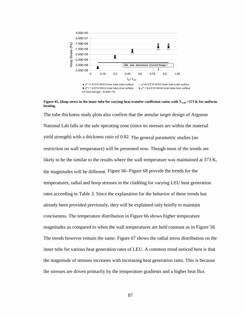
87

Figure 65. Hoop stress in the inner tube for varying heat transfer coefficient ratios with Twall =373 K for uniform

heating.

The tube thickness study plots also confirm that the annular target design of Argonne

National Lab falls in the safe operating zone (since its stresses are within the material

yield strength) with a thickness ratio of 0.82. The general parametric studies (no

restriction on wall temperature) will be presented now. Though most of the trends are

likely to be the similar to the results where the wall temperature was maintained at 373 K,

the magnitudes will be different. Figure 66- Figure 68 provide the trends for the

temperatures, radial and hoop stresses in the cladding for varying LEU heat generation

rates according to Table 3. Since the explanation for the behavior of these trends has

already been provided previously, they will be explained only briefly to maintain

conciseness. The temperature distribution in Figure 66 shows higher temperature

magnitudes as compared to when the wall temperatures are held constant as in Figure 58.

The trends however remain the same. Figure 67 shows the radial stress distribution on the

inner tube for various heat generation rates of LEU. A common trend noticed here is that

the magnitude of stresses increases with increasing heat generation rates. This is because

the stresses are driven primarily by the temperature gradients and a higher heat flux

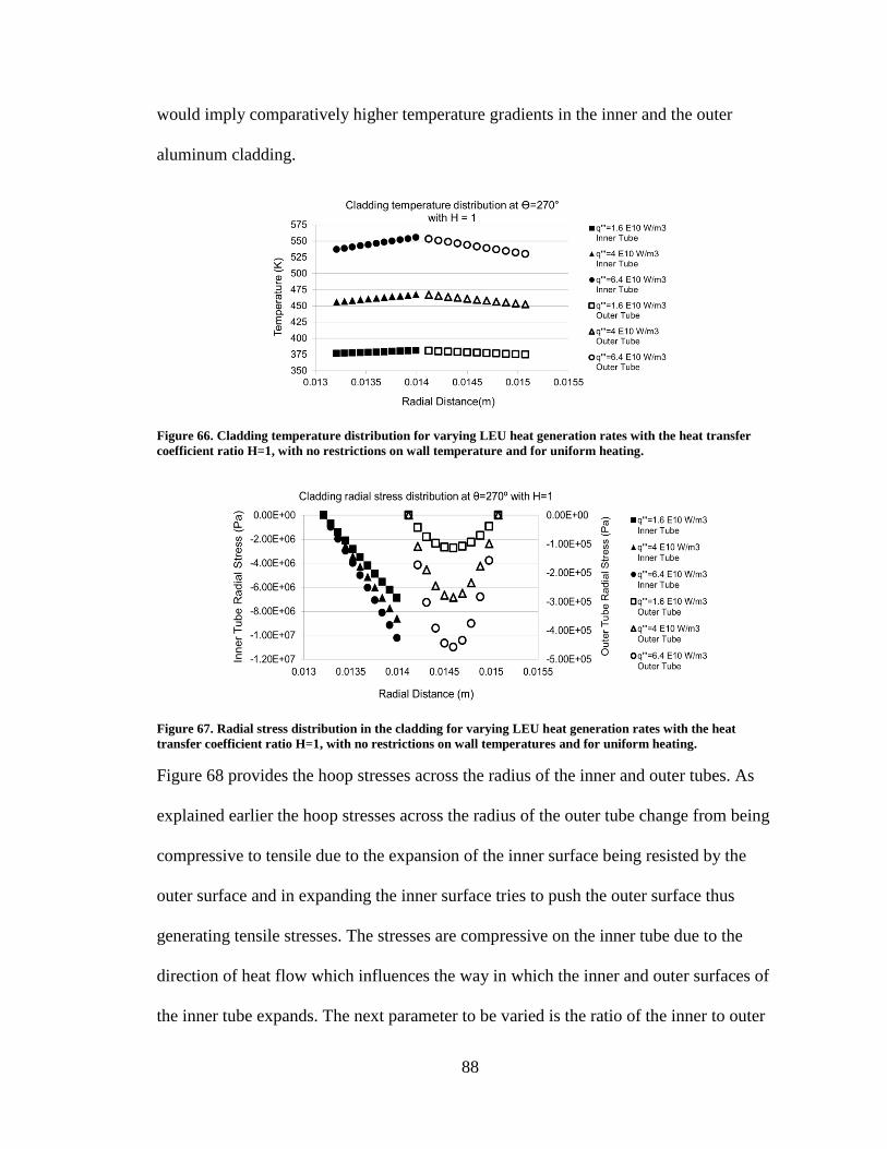
88

would imply comparatively higher temperature gradients in the inner and the outer

aluminum cladding.

Figure 66. Cladding temperature distribution for varying LEU heat generation rates with the heat transfer

coefficient ratio H=1, with no restrictions on wall temperature and for uniform heating.

Figure 67. Radial stress distribution in the cladding for varying LEU heat generation rates with the heat

transfer coefficient ratio H=1, with no restrictions on wall temperatures and for uniform heating.

Figure 68 provides the hoop stresses across the radius of the inner and outer tubes. As

explained earlier the hoop stresses across the radius of the outer tube change from being

compressive to tensile due to the expansion of the inner surface being resisted by the

outer surface and in expanding the inner surface tries to push the outer surface thus

generating tensile stresses. The stresses are compressive on the inner tube due to the

direction of heat flow which influences the way in which the inner and outer surfaces of

the inner tube expands. The next parameter to be varied is the ratio of the inner to outer

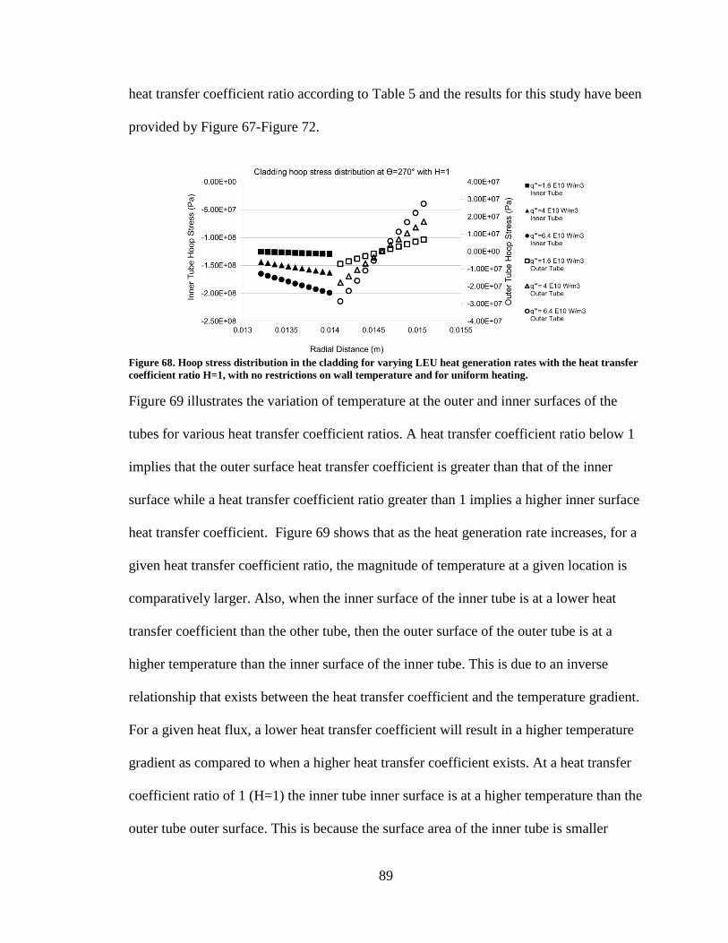
89

heat transfer coefficient ratio according to Table 5 and the results for this study have been

provided by Figure 67-Figure 72.

Figure 68. Hoop stress distribution in the cladding for varying LEU heat generation rates with the heat transfer

coefficient ratio H=1, with no restrictions on wall temperature and for uniform heating.

Figure 69 illustrates the variation of temperature at the outer and inner surfaces of the

tubes for various heat transfer coefficient ratios. A heat transfer coefficient ratio below 1

implies that the outer surface heat transfer coefficient is greater than that of the inner

surface while a heat transfer coefficient ratio greater than 1 implies a higher inner surface

heat transfer coefficient. Figure 69 shows that as the heat generation rate increases, for a

given heat transfer coefficient ratio, the magnitude of temperature at a given location is

comparatively larger. Also, when the inner surface of the inner tube is at a lower heat

transfer coefficient than the other tube, then the outer surface of the outer tube is at a

higher temperature than the inner surface of the inner tube. This is due to an inverse

relationship that exists between the heat transfer coefficient and the temperature gradient.

For a given heat flux, a lower heat transfer coefficient will result in a higher temperature

gradient as compared to when a higher heat transfer coefficient exists. At a heat transfer

coefficient ratio of 1 (H=1) the inner tube inner surface is at a higher temperature than the

outer tube outer surface. This is because the surface area of the inner tube is smaller

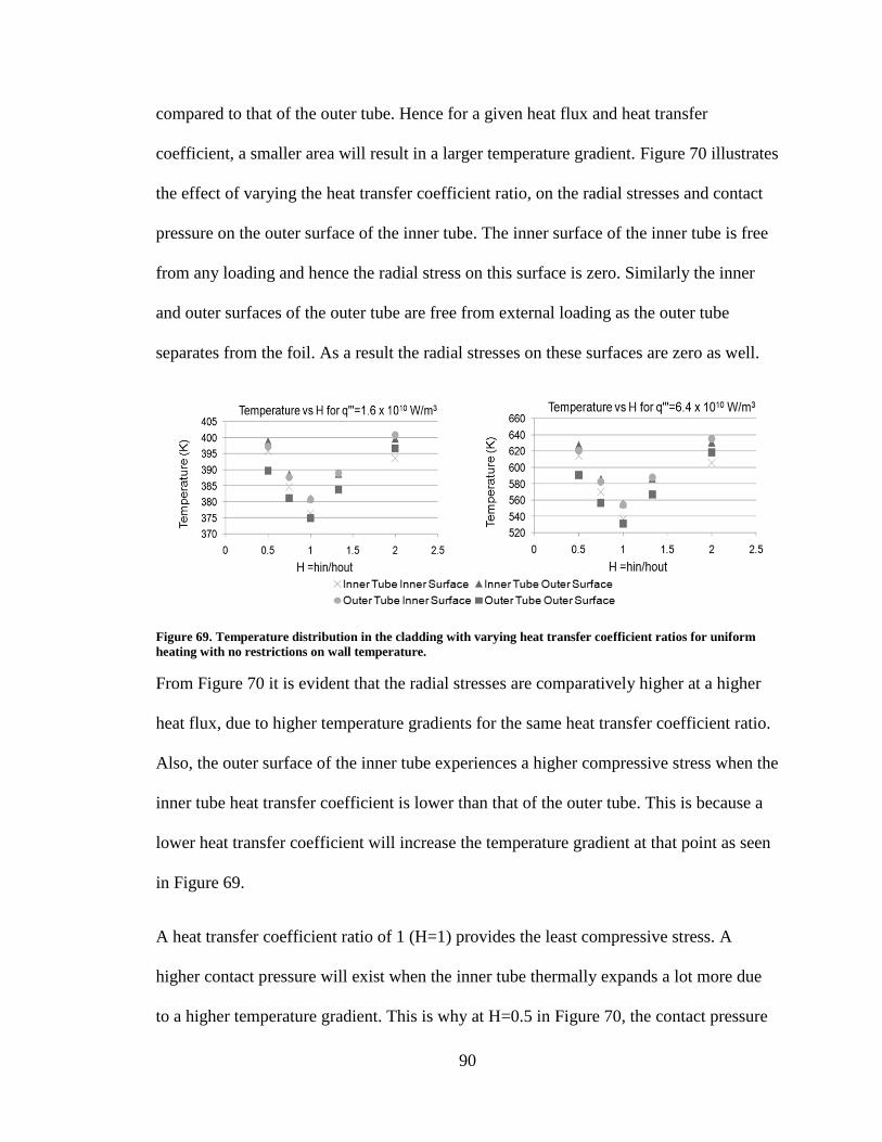
90

compared to that of the outer tube. Hence for a given heat flux and heat transfer

coefficient, a smaller area will result in a larger temperature gradient. Figure 70 illustrates

the effect of varying the heat transfer coefficient ratio, on the radial stresses and contact

pressure on the outer surface of the inner tube. The inner surface of the inner tube is free

from any loading and hence the radial stress on this surface is zero. Similarly the inner

and outer surfaces of the outer tube are free from external loading as the outer tube

separates from the foil. As a result the radial stresses on these surfaces are zero as well.

Figure 69. Temperature distribution in the cladding with varying heat transfer coefficient ratios for uniform

heating with no restrictions on wall temperature.

From Figure 70 it is evident that the radial stresses are comparatively higher at a higher

heat flux, due to higher temperature gradients for the same heat transfer coefficient ratio.

Also, the outer surface of the inner tube experiences a higher compressive stress when the

inner tube heat transfer coefficient is lower than that of the outer tube. This is because a

lower heat transfer coefficient will increase the temperature gradient at that point as seen

in Figure 69.

A heat transfer coefficient ratio of 1 (H=1) provides the least compressive stress. A

higher contact pressure will exist when the inner tube thermally expands a lot more due

to a higher temperature gradient. This is why at H=0.5 in Figure 70, the contact pressure

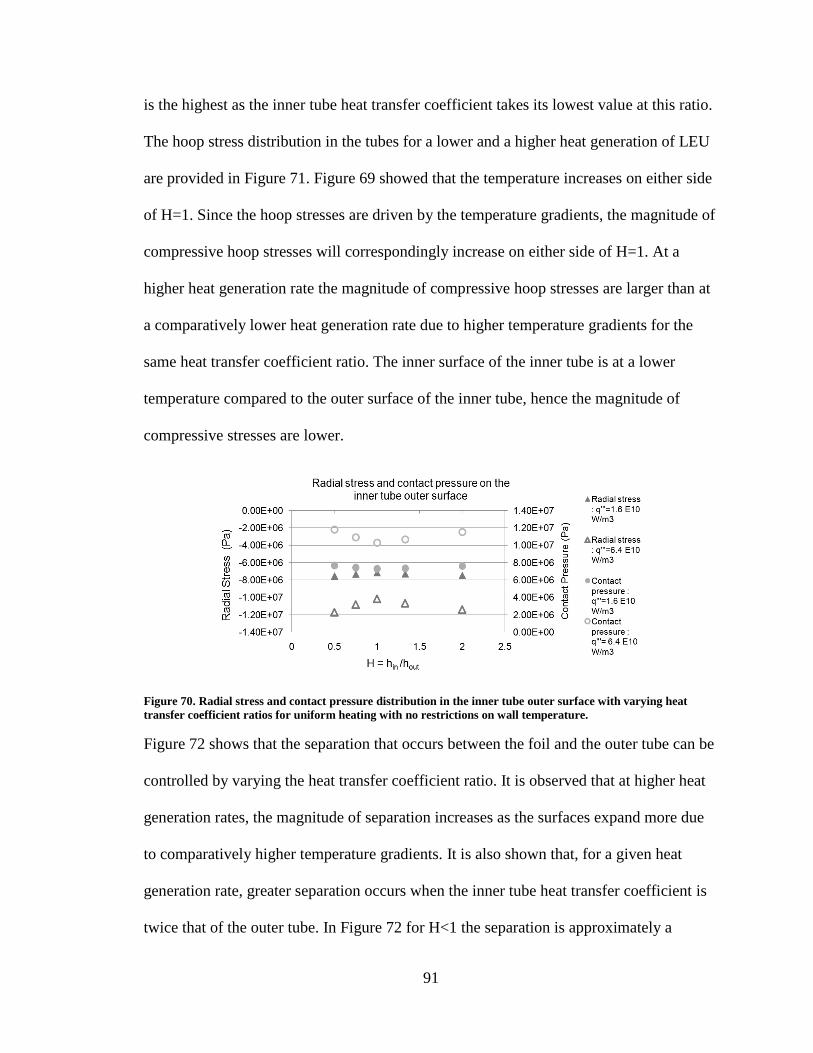
91

is the highest as the inner tube heat transfer coefficient takes its lowest value at this ratio.

The hoop stress distribution in the tubes for a lower and a higher heat generation of LEU

are provided in Figure 71. Figure 69 showed that the temperature increases on either side

of H=1. Since the hoop stresses are driven by the temperature gradients, the magnitude of

compressive hoop stresses will correspondingly increase on either side of H=1. At a

higher heat generation rate the magnitude of compressive hoop stresses are larger than at

a comparatively lower heat generation rate due to higher temperature gradients for the

same heat transfer coefficient ratio. The inner surface of the inner tube is at a lower

temperature compared to the outer surface of the inner tube, hence the magnitude of

compressive stresses are lower.

Figure 70. Radial stress and contact pressure distribution in the inner tube outer surface with varying heat

transfer coefficient ratios for uniform heating with no restrictions on wall temperature.

Figure 72 shows that the separation that occurs between the foil and the outer tube can be

controlled by varying the heat transfer coefficient ratio. It is observed that at higher heat

generation rates, the magnitude of separation increases as the surfaces expand more due

to comparatively higher temperature gradients. It is also shown that, for a given heat

generation rate, greater separation occurs when the inner tube heat transfer coefficient is

twice that of the outer tube. In Figure 72 for H<1 the separation is approximately a

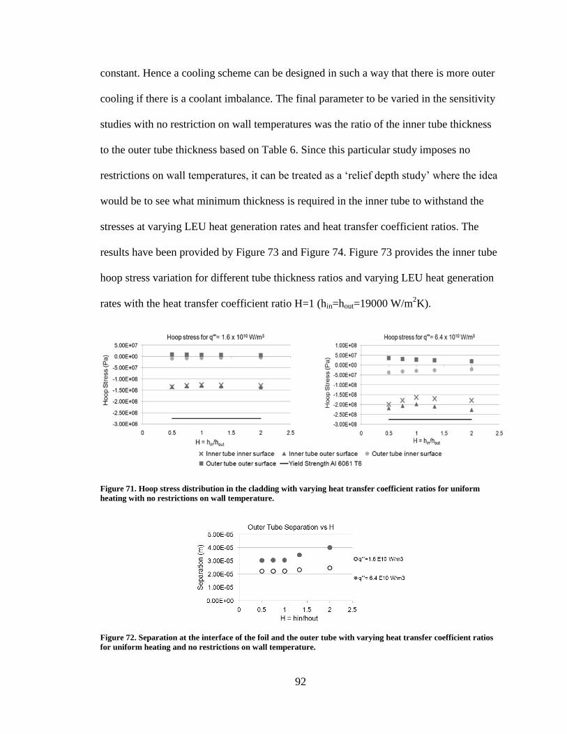
92

constant. Hence a cooling scheme can be designed in such a way that there is more outer

cooling if there is a coolant imbalance. The final parameter to be varied in the sensitivity

studies with no restriction on wall temperatures was the ratio of the inner tube thickness

to the outer tube thickness based on Table 6. Since this particular study imposes no

restrictions on wall temperatures, it can be treated as a ‘relief depth study’ where the idea

would be to see what minimum thickness is required in the inner tube to withstand the

stresses at varying LEU heat generation rates and heat transfer coefficient ratios. The

results have been provided by Figure 73 and Figure 74. Figure 73 provides the inner tube

hoop stress variation for different tube thickness ratios and varying LEU heat generation

rates with the heat transfer coefficient ratio H=1 (hin=hout=19000 W/m2K).

Figure 71. Hoop stress distribution in the cladding with varying heat transfer coefficient ratios for uniform

heating with no restrictions on wall temperature.

Figure 72. Separation at the interface of the foil and the outer tube with varying heat transfer coefficient ratios

for uniform heating and no restrictions on wall temperature.

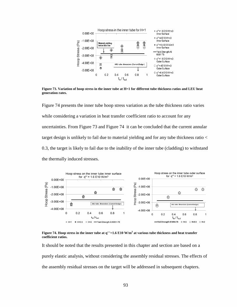
93

Figure 73. Variation of hoop stress in the inner tube at H=1 for different tube thickness ratios and LEU heat

generation rates.

Figure 74 presents the inner tube hoop stress variation as the tube thickness ratio varies

while considering a variation in heat transfer coefficient ratio to account for any

uncertainties. From Figure 73 and Figure 74 it can be concluded that the current annular

target design is unlikely to fail due to material yielding and for any tube thickness ratio <

0.3, the target is likely to fail due to the inability of the inner tube (cladding) to withstand

the thermally induced stresses.

Figure 74. Hoop stress in the inner tube at q'''=1.6 E10 W/m3 at various tube thickness and heat transfer

coefficient ratios.

It should be noted that the results presented in this chapter and section are based on a

purely elastic analysis, without considering the assembly residual stresses. The effects of

the assembly residual stresses on the target will be addressed in subsequent chapters.

94

Chapter 6: Dimensionless Analytical Model- Uniform Heating

The dimensional form of the analytical model for uniform heating in a three layer annular

cylinder in Sec. 4.3 is difficult to reproduce considering the length of the equations

presented. It was decided to present those models in dimensionless form, which would

make them more general and usable for design purposes, irrespective of the geometry and

heat generation rates. The concept of thermal expansion mismatch has been used to

develop an axisymmetric, non-dimensional, analytic solution, to predict the thermal

mechanical behavior in a three layer composite cylinder. The middle cylinder represents

the heat generating source and its thermal expansion coefficient being lesser than that of

the two cylinders enclosing it. The development of the solution is based on the

assumption that the separation occurs at the interface of the middle cylinder and the outer

cylinder, while contact is reinforced between the middle cylinder and the inner cylinder.

If the middle cylinder is assumed to be the uranium foil and the two cylinders enclosing it

as the aluminum cladding, this dimensionless model can be applied to the current annular

target configuration for a uniform heating condition.

6.1 Dimensionless Thermal-Mechanical Expressions

The dimensional form of the temperature and stresses, for the approach presented in

Figure 26, is given by Eqs.(18)-(43). The following dimensionless quantities, given by

Eq. (48), are used in developing the dimensionless expressions for the temperature

distribution, interface temperature, radial stress, hoop stress, displacement and interface

stress as given by Eqs. (49)- (54) respectively.

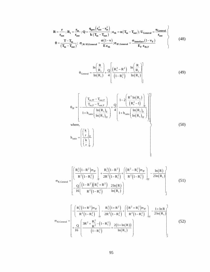
95

2 2

,/,

; ; ; ;

1 1; ;

gen out in Generalint th in out General

out out in out out

Interface FinIF GeneralR H General

in out th F th F

q r r urrR R Q T T U

r r k T T r

T T

T T E E

(48)

2 2tt t

General 2t tt

R Rln ln

R RR RQ

ln R 4 ln R1 R

(49)

2t

in,IT out,F2tin,F out,F F

IF

t tF Fratio ratio

t tIT IT

ITratio

F

R ln RT T 1 2R 1T T Q

4ln R ln R1 h 1 h

ln R ln R

where,

k

rh

k

r

(50)

2 2 2 2 2 2t IF t t IF

2 2 2 2 2 2tt t t

F ITR,General

2 2 2t

2 2tt

R 1 R R 1 R R R ln R

2ln RR 1 R 2R 1 R R 1 R

1 R R R 2ln RQ

16 ln RR 1 R

(51)

2 2 2 2 2 2t IF t t IF

2 2 2 2 2 2tt t t

F IT

2H,General 2 2t

t2

2tt

R 1 R R 1 R R R 1 ln R

2ln RR 1 R 2R 1 R R 1 R

R3R 1 R 2 1 ln RQ R

16 ln R1 R

(52)

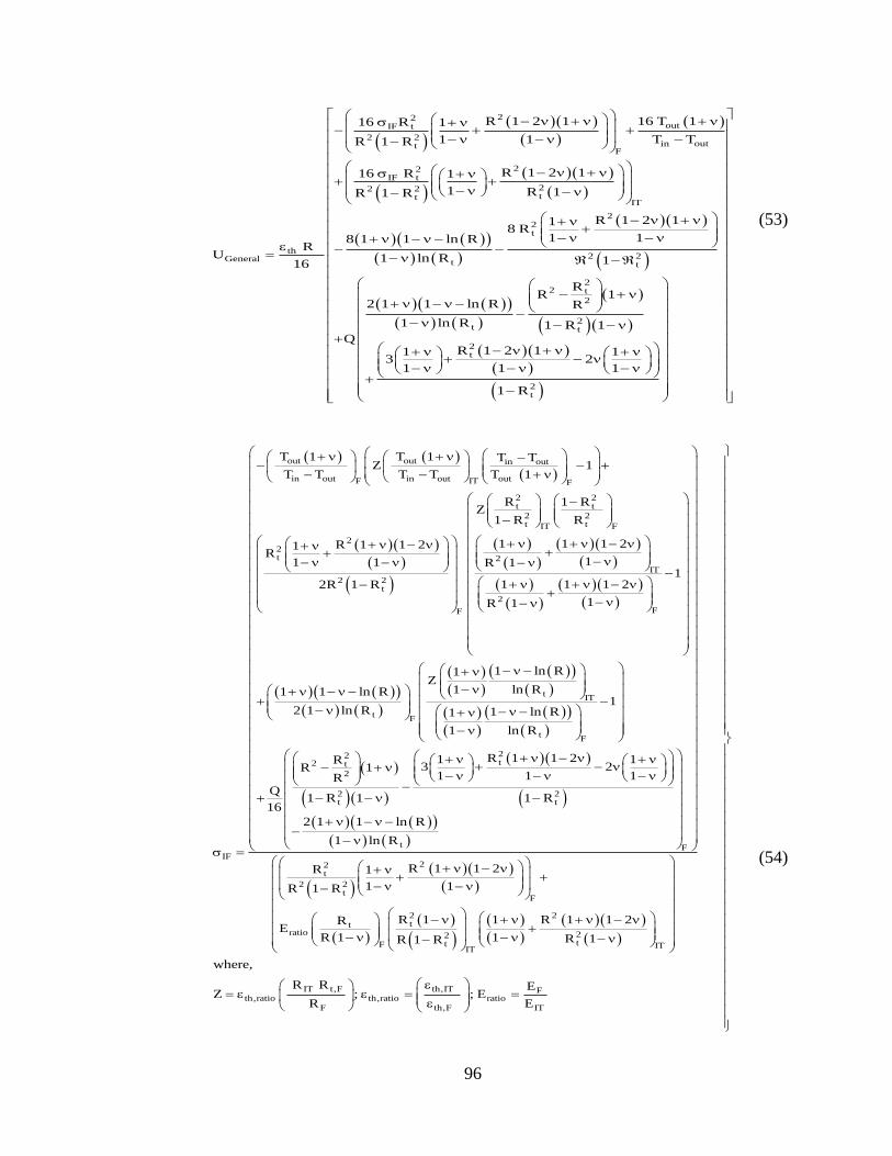
96

22outIF t

2 2in outt

F

22IF t

22 2tt

IT

22t

th2General t

R 1 2 1 16 T 116 R 1

1 1 T TR 1 R

R 1 2 116 R 1

1 R 1R 1 R

R 1 2 118 R

1 18 1 1 ln RR

U 1 ln R16

2t

22 t

2

2t t

2t

2t

1

RR 1

2 1 1 ln R R

1 ln R 1 R 1

QR 1 2 11 1

3 21 1 1

1 R

(53)

out out in out

in out in out outF IT F

2 2t t

2 2t tIT F

22t 2

2 2t

F

IF

T 1 T 1 T TZ 1

T T T T T 1

R 1 RZ

1 R R

1 1 1 2R 1 1 21R

11 1 R 1

2R 1 R

IT

2

F

tIT

tF

tF

22 t

2

2t

11 1 1 2

1R 1

1 ln R1Z

1 ln R1 1 ln R1

2 1 ln R 1 ln R1

1 ln R

1R3R 1

RQ

1 R 116

2t

2t

t F

22t

2 2t

R 1 1 2 12

1 1 1

1 R

2 1 1 ln R

1 ln R

R 1 1 2R 1

1 1R 1 R

F

2 2tt

ratio 22ttF IT

IT

IT t,F th,IT Fth,ratio th,ratio ratio

F th,F IT

R 1 1 R 1 1 2RE

R 1 1 R 1R 1 R

where,

R R EZ ; ; E

R E

(54)

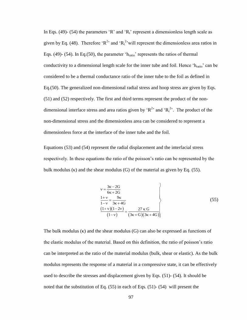
97

In Eqs. (49)- (54) the parameters ‘R’ and ‘Rt’ represent a dimensionless length scale as

given by Eq. (48). Therefore ‘R2’ and ‘Rt

2’will represent the dimensionless area ratios in

Eqs. (49)- (54). In Eq.(50), the parameter ‘hratio’ represents the ratios of thermal

conductivity to a dimensional length scale for the inner tube and foil. Hence ‘hratio’ can be

considered to be a thermal conductance ratio of the inner tube to the foil as defined in

Eq.(50). The generalized non-dimensional radial stress and hoop stress are given by Eqs.

(51) and (52) respectively. The first and third terms represent the product of the non-

dimensional interface stress and area ratios given by ‘R2’ and ‘Rt

2’. The product of the

non-dimensional stress and the dimensionless area can be considered to represent a

dimensionless force at the interface of the inner tube and the foil.

Equations (53) and (54) represent the radial displacement and the interfacial stress

respectively. In these equations the ratio of the poisson’s ratio can be represented by the

bulk modulus (κ) and the shear modulus (G) of the material as given by Eq. (55).

3 2G

6 2G

1 9

1 3 4G

1 1 2 27 G

1 3 G 3 4G

(55)

The bulk modulus (κ) and the shear modulus (G) can also be expressed as functions of

the elastic modulus of the material. Based on this definition, the ratio of poisson’s ratio

can be interpreted as the ratio of the material modulus (bulk, shear or elastic). As the bulk

modulus represents the response of a material in a compressive state, it can be effectively

used to describe the stresses and displacement given by Eqs. (51)- (54). It should be

noted that the substitution of Eq. (55) in each of Eqs. (51)- (54) will present the

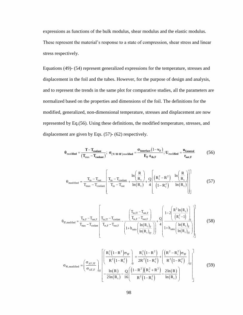
98

expressions as functions of the bulk modulus, shear modulus and the elastic modulus.

These represent the material’s response to a state of compression, shear stress and linear

stress respectively.

Equations (49)- (54) represent generalized expressions for the temperature, stresses and

displacement in the foil and the tubes. However, for the purpose of design and analysis,

and to represent the trends in the same plot for comparative studies, all the parameters are

normalized based on the properties and dimensions of the foil. The definitions for the

modified, generalized, non-dimensional temperature, stresses and displacement are now

represented by Eq.(56). Using these definitions, the modified temperature, stresses, and

displacement are given by Eqs. (57)- (62) respectively.

mod mod/ / mod

max , ,

1; ;

Interface Fcoolant Generalified ifiedH IF ified

coolant F th F out F

T T uU

T T E r

(56)

2 2tt tin out in coolant

modified 2max coolant in out t tt

R Rln ln

R RR RT T T T Q

T T T T ln R 4 ln R1 R

(57)

2t

in,IT out,F2tin,F out,Fin,F out,F in,IT coolant F

IF,modifiedmax coolant in,F out,F tt FF

ratioratiott ITIT

R ln RT T 1 2R 1T TT T T T Q

T T T T 4 ln Rln R1 h1 h

ln Rln R

(58)

2 2 2 2 2 2t IF t t IF

2 2 2 2 2 2t t t

T,IT F IT,modified

2 2 2T,F IT t

2 2t tt

R 1 R R 1 R R R

R 1 R 2R 1 R R 1 R

1 R R Rln R 2ln RQ

2ln R 16 ln RR 1 R

(59)

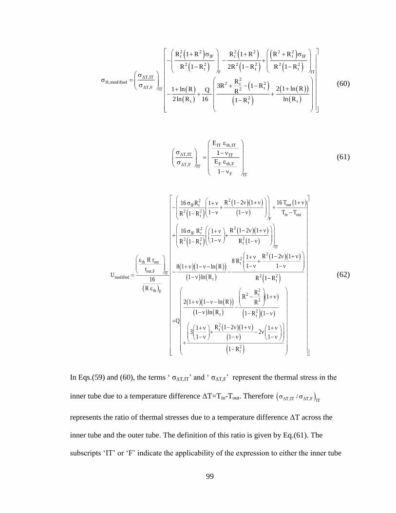
99

2 2 2 2 2 2t IF t t IF

2 2 2 2 2 2t t t

F IT

T,IT 2H,modified 2 2t

T,F t2IT

2t tt

R 1 R R 1 R R R

R 1 R 2R 1 R R 1 R

R3R 1 R 2 1 ln R1 ln R Q R

2ln R 16 ln R1 R

(60)

IT th,IT

T,IT IT

F th,FT,F IT

F IT

E

1

E

1

(61)

22outIF t

2 2in outt

F

22IF t

22 2tt

IT

2th out t

out,F ITmodified t

th F

R 1 2 1 16 T 116 R 1

1 1 T TR 1 R

R 1 2 116 R 1

1 R 1R 1 R

1R r 8 R8 1 1 ln Rr

U 1 ln R16

R

2

2 2t

22 t

2

2t t

2t

2t

R 1 2 1

1 1

R 1 R

RR 1

2 1 1 ln R R

1 ln R 1 R 1

QR 1 2 11 1

3 21 1 1

1 R

(62)

In Eqs.(59) and (60), the terms ‘ σΔT,IT’ and ‘ σΔT,F’ represent the thermal stress in the

inner tube due to a temperature difference ΔT=Tin-Tout. Therefore T,IT T,F IT/

represents the ratio of thermal stresses due to a temperature difference ΔT across the

inner tube and the outer tube. The definition of this ratio is given by Eq.(61). The

subscripts ‘IT’ or ‘F’ indicate the applicability of the expression to either the inner tube

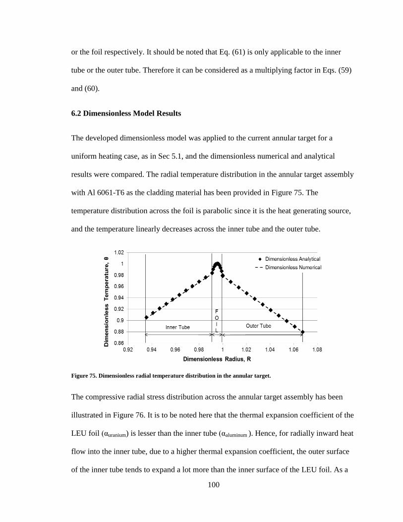
100

or the foil respectively. It should be noted that Eq. (61) is only applicable to the inner

tube or the outer tube. Therefore it can be considered as a multiplying factor in Eqs. (59)

and (60).

6.2 Dimensionless Model Results

The developed dimensionless model was applied to the current annular target for a

uniform heating case, as in Sec 5.1, and the dimensionless numerical and analytical

results were compared. The radial temperature distribution in the annular target assembly

with Al 6061-T6 as the cladding material has been provided in Figure 75. The

temperature distribution across the foil is parabolic since it is the heat generating source,

and the temperature linearly decreases across the inner tube and the outer tube.

Figure 75. Dimensionless radial temperature distribution in the annular target.

The compressive radial stress distribution across the annular target assembly has been

illustrated in Figure 76. It is to be noted here that the thermal expansion coefficient of the

LEU foil (αuranium) is lesser than the inner tube (αaluminum ). Hence, for radially inward heat

flow into the inner tube, due to a higher thermal expansion coefficient, the outer surface

of the inner tube tends to expand a lot more than the inner surface of the LEU foil. As a

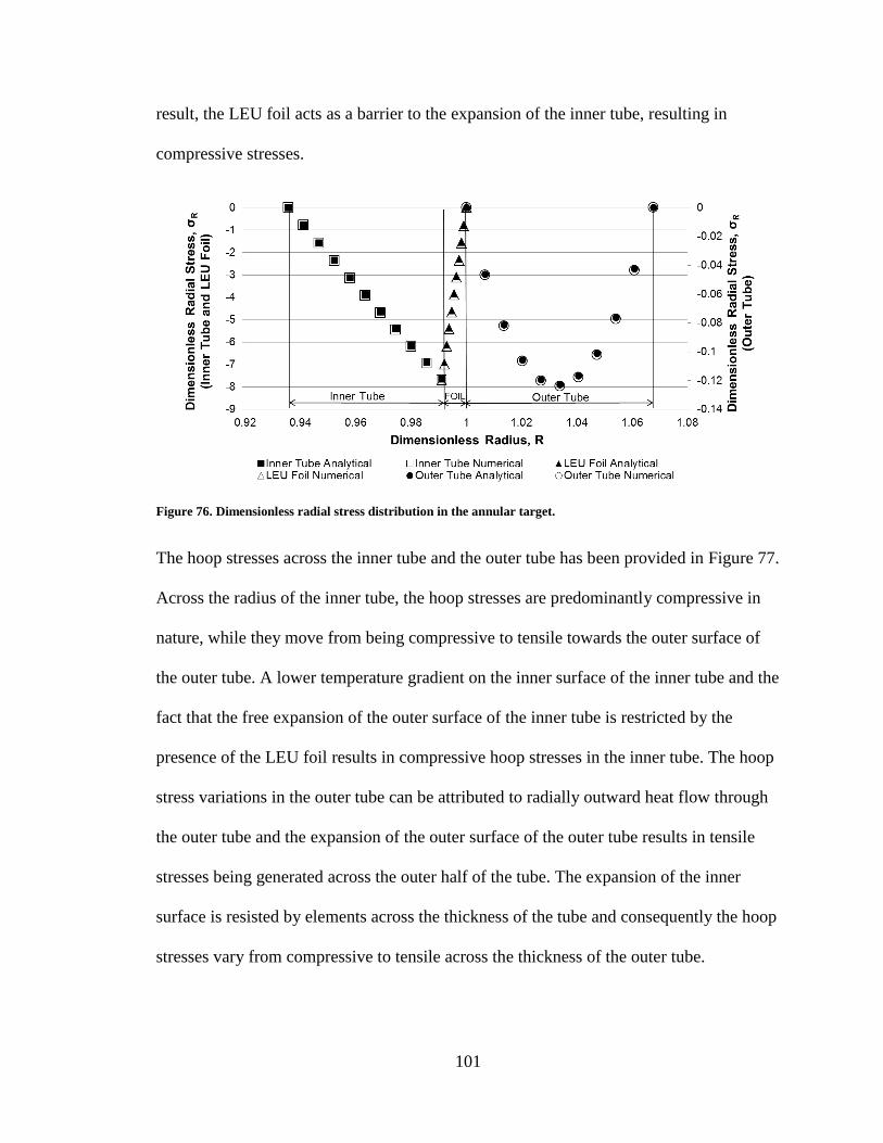
101

result, the LEU foil acts as a barrier to the expansion of the inner tube, resulting in

compressive stresses.

Figure 76. Dimensionless radial stress distribution in the annular target.

The hoop stresses across the inner tube and the outer tube has been provided in Figure 77.

Across the radius of the inner tube, the hoop stresses are predominantly compressive in

nature, while they move from being compressive to tensile towards the outer surface of

the outer tube. A lower temperature gradient on the inner surface of the inner tube and the

fact that the free expansion of the outer surface of the inner tube is restricted by the

presence of the LEU foil results in compressive hoop stresses in the inner tube. The hoop

stress variations in the outer tube can be attributed to radially outward heat flow through

the outer tube and the expansion of the outer surface of the outer tube results in tensile

stresses being generated across the outer half of the tube. The expansion of the inner

surface is resisted by elements across the thickness of the tube and consequently the hoop

stresses vary from compressive to tensile across the thickness of the outer tube.

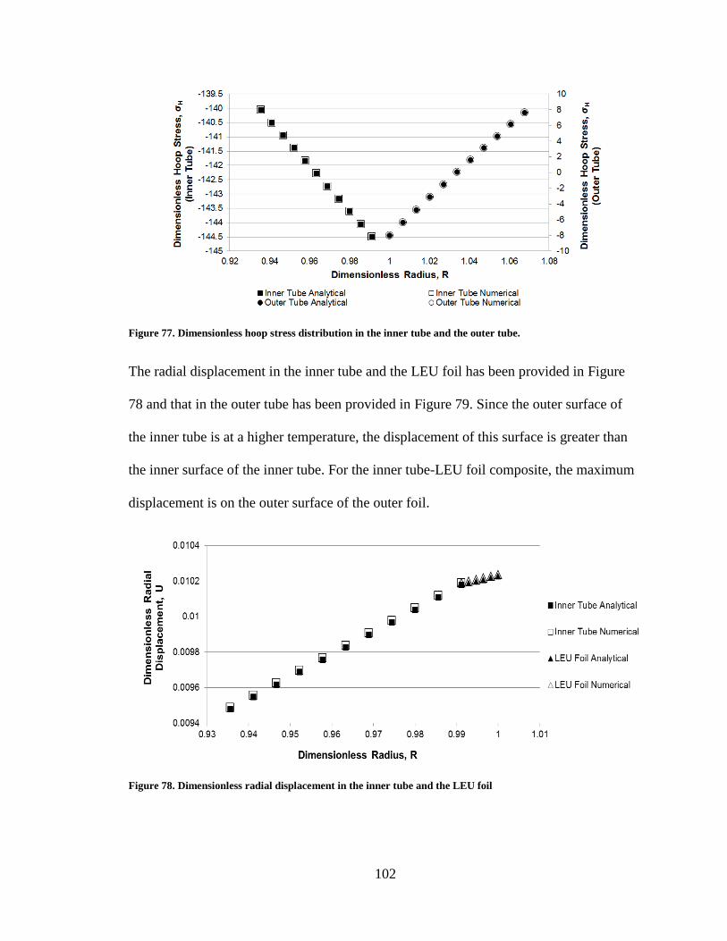
102

Figure 77. Dimensionless hoop stress distribution in the inner tube and the outer tube.

The radial displacement in the inner tube and the LEU foil has been provided in Figure

78 and that in the outer tube has been provided in Figure 79. Since the outer surface of

the inner tube is at a higher temperature, the displacement of this surface is greater than

the inner surface of the inner tube. For the inner tube-LEU foil composite, the maximum

displacement is on the outer surface of the outer foil.

Figure 78. Dimensionless radial displacement in the inner tube and the LEU foil

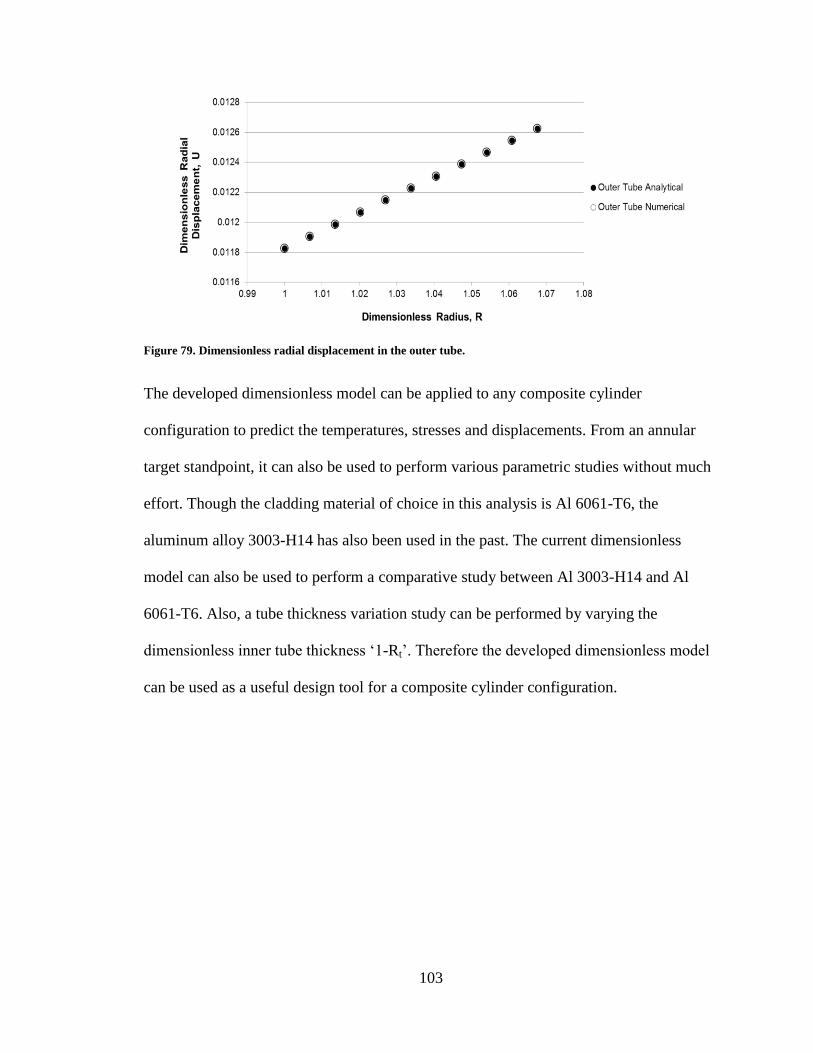
103

Figure 79. Dimensionless radial displacement in the outer tube.

The developed dimensionless model can be applied to any composite cylinder

configuration to predict the temperatures, stresses and displacements. From an annular

target standpoint, it can also be used to perform various parametric studies without much

effort. Though the cladding material of choice in this analysis is Al 6061-T6, the

aluminum alloy 3003-H14 has also been used in the past. The current dimensionless

model can also be used to perform a comparative study between Al 3003-H14 and Al

6061-T6. Also, a tube thickness variation study can be performed by varying the

dimensionless inner tube thickness ‘1-Rt’. Therefore the developed dimensionless model

can be used as a useful design tool for a composite cylinder configuration.

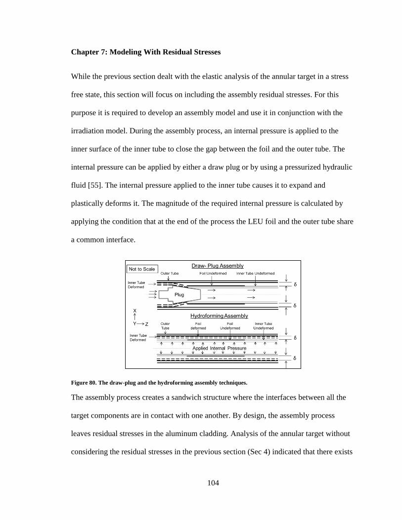
104

Chapter 7: Modeling With Residual Stresses

While the previous section dealt with the elastic analysis of the annular target in a stress

free state, this section will focus on including the assembly residual stresses. For this

purpose it is required to develop an assembly model and use it in conjunction with the

irradiation model. During the assembly process, an internal pressure is applied to the

inner surface of the inner tube to close the gap between the foil and the outer tube. The

internal pressure can be applied by either a draw plug or by using a pressurized hydraulic

fluid [55]. The internal pressure applied to the inner tube causes it to expand and

plastically deforms it. The magnitude of the required internal pressure is calculated by

applying the condition that at the end of the process the LEU foil and the outer tube share

a common interface.

Figure 80. The draw-plug and the hydroforming assembly techniques.

The assembly process creates a sandwich structure where the interfaces between all the

target components are in contact with one another. By design, the assembly process

leaves residual stresses in the aluminum cladding. Analysis of the annular target without

considering the residual stresses in the previous section (Sec 4) indicated that there exists

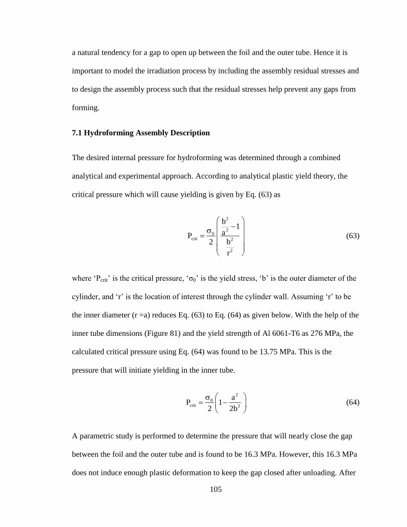
105

a natural tendency for a gap to open up between the foil and the outer tube. Hence it is

important to model the irradiation process by including the assembly residual stresses and

to design the assembly process such that the residual stresses help prevent any gaps from

forming.

7.1 Hydroforming Assembly Description

The desired internal pressure for hydroforming was determined through a combined

analytical and experimental approach. According to analytical plastic yield theory, the

critical pressure which will cause yielding is given by Eq. (63) as

2

20

crit 2

2

b1

aPb2

r

(63)

where ‘Pcrit’ is the critical pressure, ‘σ0’ is the yield stress, ‘b’ is the outer diameter of the

cylinder, and ‘r’ is the location of interest through the cylinder wall. Assuming ‘r’ to be

the inner diameter (r =a) reduces Eq. (63) to Eq. (64) as given below. With the help of the

inner tube dimensions (Figure 81) and the yield strength of Al 6061-T6 as 276 MPa, the

calculated critical pressure using Eq. (64) was found to be 13.75 MPa. This is the

pressure that will initiate yielding in the inner tube.

2

0crit 2

aP 1

2 2b

(64)

A parametric study is performed to determine the pressure that will nearly close the gap

between the foil and the outer tube and is found to be 16.3 MPa. However, this 16.3 MPa

does not induce enough plastic deformation to keep the gap closed after unloading. After

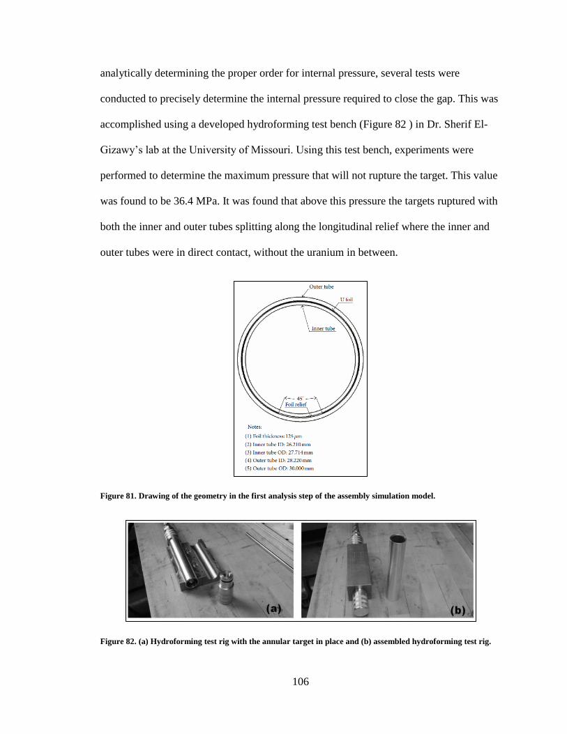
106

analytically determining the proper order for internal pressure, several tests were

conducted to precisely determine the internal pressure required to close the gap. This was

accomplished using a developed hydroforming test bench (Figure 82 ) in Dr. Sherif El-

Gizawy’s lab at the University of Missouri. Using this test bench, experiments were

performed to determine the maximum pressure that will not rupture the target. This value

was found to be 36.4 MPa. It was found that above this pressure the targets ruptured with

both the inner and outer tubes splitting along the longitudinal relief where the inner and

outer tubes were in direct contact, without the uranium in between.

Figure 81. Drawing of the geometry in the first analysis step of the assembly simulation model.

Figure 82. (a) Hydroforming test rig with the annular target in place and (b) assembled hydroforming test rig.

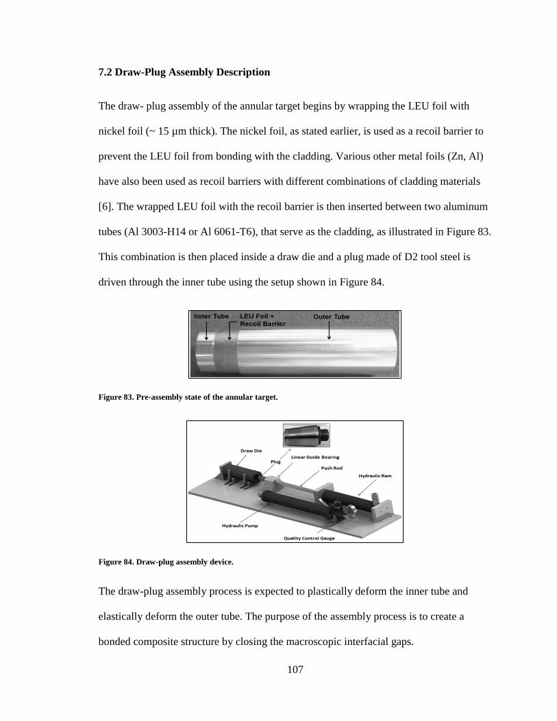
107

7.2 Draw-Plug Assembly Description

The draw- plug assembly of the annular target begins by wrapping the LEU foil with

nickel foil (~ 15 µm thick). The nickel foil, as stated earlier, is used as a recoil barrier to

prevent the LEU foil from bonding with the cladding. Various other metal foils (Zn, Al)

have also been used as recoil barriers with different combinations of cladding materials

[6]. The wrapped LEU foil with the recoil barrier is then inserted between two aluminum

tubes (Al 3003-H14 or Al 6061-T6), that serve as the cladding, as illustrated in Figure 83.

This combination is then placed inside a draw die and a plug made of D2 tool steel is

driven through the inner tube using the setup shown in Figure 84.

Figure 83. Pre-assembly state of the annular target.

Figure 84. Draw-plug assembly device.

The draw-plug assembly process is expected to plastically deform the inner tube and

elastically deform the outer tube. The purpose of the assembly process is to create a

bonded composite structure by closing the macroscopic interfacial gaps.

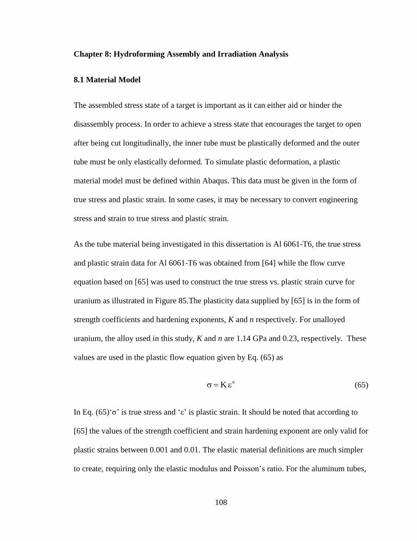
108

Chapter 8: Hydroforming Assembly and Irradiation Analysis

8.1 Material Model

The assembled stress state of a target is important as it can either aid or hinder the

disassembly process. In order to achieve a stress state that encourages the target to open

after being cut longitudinally, the inner tube must be plastically deformed and the outer

tube must be only elastically deformed. To simulate plastic deformation, a plastic

material model must be defined within Abaqus. This data must be given in the form of

true stress and plastic strain. In some cases, it may be necessary to convert engineering

stress and strain to true stress and plastic strain.

As the tube material being investigated in this dissertation is Al 6061-T6, the true stress

and plastic strain data for Al 6061-T6 was obtained from [64] while the flow curve

equation based on [65] was used to construct the true stress vs. plastic strain curve for

uranium as illustrated in Figure 85.The plasticity data supplied by [65] is in the form of

strength coefficients and hardening exponents, K and n respectively. For unalloyed

uranium, the alloy used in this study, K and n are 1.14 GPa and 0.23, respectively. These

values are used in the plastic flow equation given by Eq. (65) as

nK (65)

In Eq. (65)‘σ’ is true stress and ‘ε’ is plastic strain. It should be noted that according to

[65] the values of the strength coefficient and strain hardening exponent are only valid for

plastic strains between 0.001 and 0.01. The elastic material definitions are much simpler

to create, requiring only the elastic modulus and Poisson’s ratio. For the aluminum tubes,

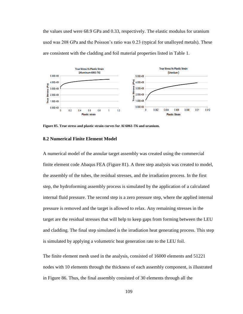
109

the values used were 68.9 GPa and 0.33, respectively. The elastic modulus for uranium

used was 208 GPa and the Poisson’s ratio was 0.23 (typical for unalloyed metals). These

are consistent with the cladding and foil material properties listed in Table 1.

Figure 85. True stress and plastic strain curves for Al 6061-T6 and uranium.

8.2 Numerical Finite Element Model

A numerical model of the annular target assembly was created using the commercial

finite element code Abaqus FEA (Figure 81). A three step analysis was created to model,

the assembly of the tubes, the residual stresses, and the irradiation process. In the first

step, the hydroforming assembly process is simulated by the application of a calculated

internal fluid pressure. The second step is a zero pressure step, where the applied internal

pressure is removed and the target is allowed to relax. Any remaining stresses in the

target are the residual stresses that will help to keep gaps from forming between the LEU

and cladding. The final step simulated is the irradiation heat generating process. This step

is simulated by applying a volumetric heat generation rate to the LEU foil.

The finite element mesh used in the analysis, consisted of 16000 elements and 51221

nodes with 10 elements through the thickness of each assembly component, is illustrated

in Figure 86. Thus, the final assembly consisted of 30 elements through all the

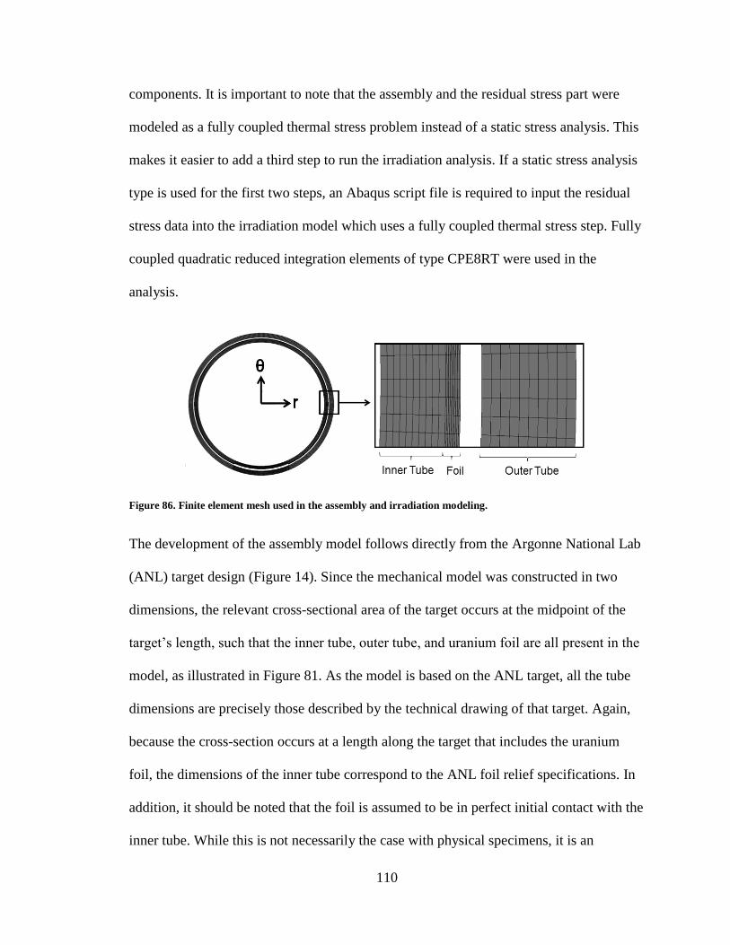
110

components. It is important to note that the assembly and the residual stress part were

modeled as a fully coupled thermal stress problem instead of a static stress analysis. This

makes it easier to add a third step to run the irradiation analysis. If a static stress analysis

type is used for the first two steps, an Abaqus script file is required to input the residual

stress data into the irradiation model which uses a fully coupled thermal stress step. Fully

coupled quadratic reduced integration elements of type CPE8RT were used in the

analysis.

Figure 86. Finite element mesh used in the assembly and irradiation modeling.

The development of the assembly model follows directly from the Argonne National Lab

(ANL) target design (Figure 14). Since the mechanical model was constructed in two

dimensions, the relevant cross-sectional area of the target occurs at the midpoint of the

target’s length, such that the inner tube, outer tube, and uranium foil are all present in the

model, as illustrated in Figure 81. As the model is based on the ANL target, all the tube

dimensions are precisely those described by the technical drawing of that target. Again,

because the cross-section occurs at a length along the target that includes the uranium

foil, the dimensions of the inner tube correspond to the ANL foil relief specifications. In

addition, it should be noted that the foil is assumed to be in perfect initial contact with the

inner tube. While this is not necessarily the case with physical specimens, it is an

111

essential simplification to the model. The loading and boundary conditions for the

assembly model have been provided in Figure 87. The calculated maximum allowable

pressure using the hydroforming test bench experiments of 36.4 MPa was applied as an

internal pressure to the annular target as shown in Figure 87.

Figure 87. Loading and mechanical boundary conditions for the assembly hydroforming simulation in the first

analysis step.

To model the irradiation behavior which takes into account the residual stresses from the

assembly process, a fully coupled thermal stress step was added after the residual stress

step. The loading conditions and the contact definitions from the first two steps were

suppressed. A heat generation rate of 1.6 x 1010

W/m3

was applied to the foil, which

corresponds to a heat flux of 100 W/cm2incident on the outer surface of the inner tube

and the inner surface of the outer tube. Water coolant flow at 323 K through the inner and

along the outer tubes was simulated by defining a surface heat transfer coefficient and a

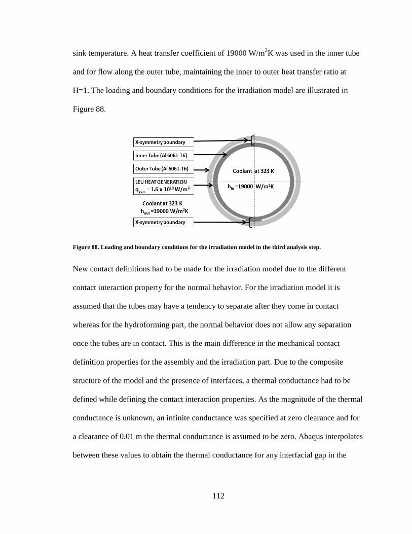
112

sink temperature. A heat transfer coefficient of 19000 W/m2K was used in the inner tube

and for flow along the outer tube, maintaining the inner to outer heat transfer ratio at

H=1. The loading and boundary conditions for the irradiation model are illustrated in

Figure 88.

Figure 88. Loading and boundary conditions for the irradiation model in the third analysis step.

New contact definitions had to be made for the irradiation model due to the different

contact interaction property for the normal behavior. For the irradiation model it is

assumed that the tubes may have a tendency to separate after they come in contact

whereas for the hydroforming part, the normal behavior does not allow any separation

once the tubes are in contact. This is the main difference in the mechanical contact

definition properties for the assembly and the irradiation part. Due to the composite

structure of the model and the presence of interfaces, a thermal conductance had to be

defined while defining the contact interaction properties. As the magnitude of the thermal

conductance is unknown, an infinite conductance was specified at zero clearance and for

a clearance of 0.01 m the thermal conductance is assumed to be zero. Abaqus interpolates

between these values to obtain the thermal conductance for any interfacial gap in the

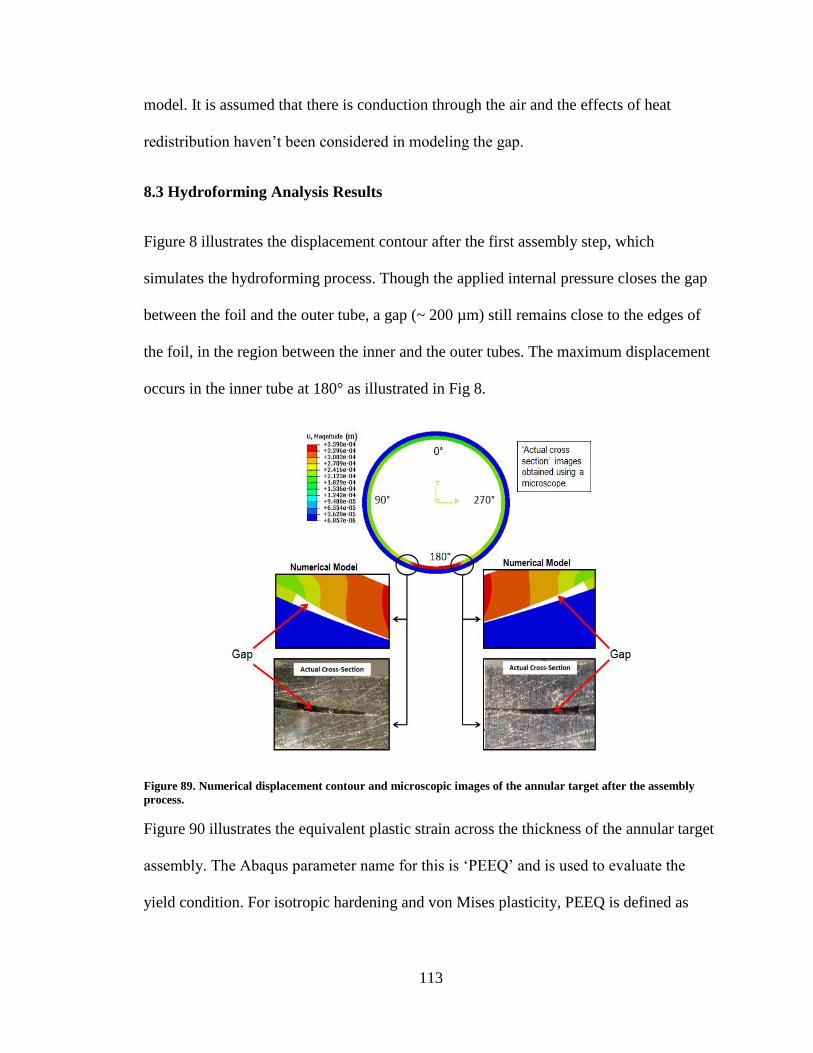
113

model. It is assumed that there is conduction through the air and the effects of heat

redistribution haven’t been considered in modeling the gap.

8.3 Hydroforming Analysis Results

Figure 8 illustrates the displacement contour after the first assembly step, which

simulates the hydroforming process. Though the applied internal pressure closes the gap

between the foil and the outer tube, a gap (~ 200 µm) still remains close to the edges of

the foil, in the region between the inner and the outer tubes. The maximum displacement

occurs in the inner tube at 180° as illustrated in Fig 8.

Figure 89. Numerical displacement contour and microscopic images of the annular target after the assembly

process.

Figure 90 illustrates the equivalent plastic strain across the thickness of the annular target

assembly. The Abaqus parameter name for this is ‘PEEQ’ and is used to evaluate the

yield condition. For isotropic hardening and von Mises plasticity, PEEQ is defined as

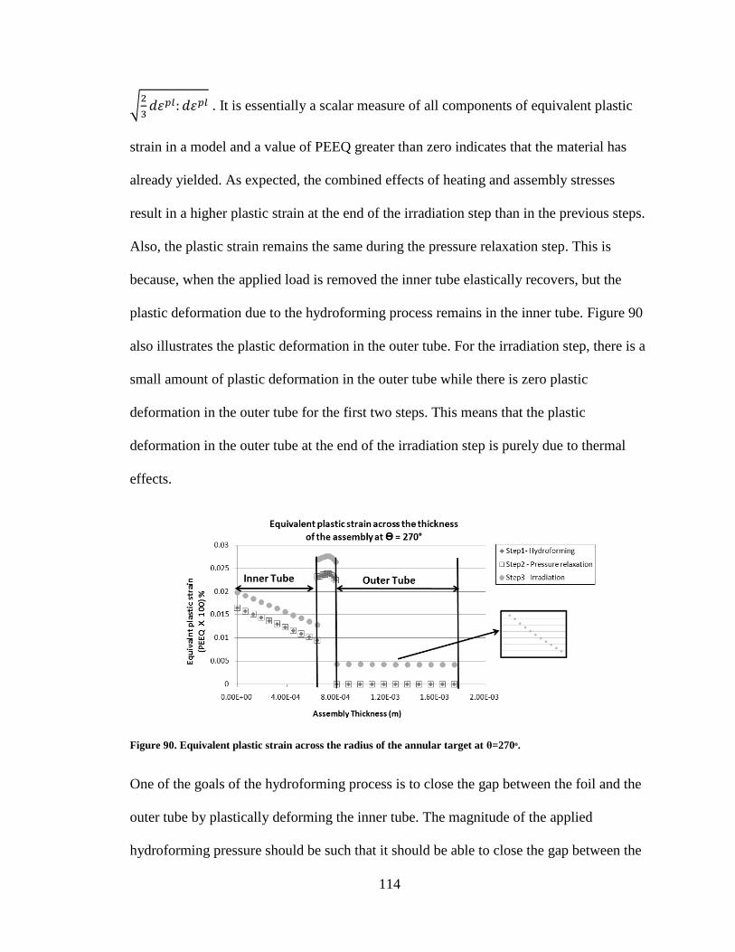
114

√2

3𝑑𝜀𝑝𝑙: 𝑑𝜀𝑝𝑙 . It is essentially a scalar measure of all components of equivalent plastic

strain in a model and a value of PEEQ greater than zero indicates that the material has

already yielded. As expected, the combined effects of heating and assembly stresses

result in a higher plastic strain at the end of the irradiation step than in the previous steps.

Also, the plastic strain remains the same during the pressure relaxation step. This is

because, when the applied load is removed the inner tube elastically recovers, but the

plastic deformation due to the hydroforming process remains in the inner tube. Figure 90

also illustrates the plastic deformation in the outer tube. For the irradiation step, there is a

small amount of plastic deformation in the outer tube while there is zero plastic

deformation in the outer tube for the first two steps. This means that the plastic

deformation in the outer tube at the end of the irradiation step is purely due to thermal

effects.

Figure 90. Equivalent plastic strain across the radius of the annular target at θ=270ᵒ.

One of the goals of the hydroforming process is to close the gap between the foil and the

outer tube by plastically deforming the inner tube. The magnitude of the applied

hydroforming pressure should be such that it should be able to close the gap between the

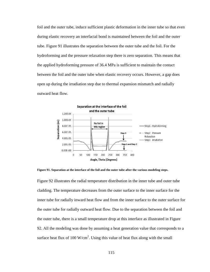
115

foil and the outer tube, induce sufficient plastic deformation in the inner tube so that even

during elastic recovery an interfacial bond is maintained between the foil and the outer

tube. Figure 91 illustrates the separation between the outer tube and the foil. For the

hydroforming and the pressure relaxation step there is zero separation. This means that

the applied hydroforming pressure of 36.4 MPa is sufficient to maintain the contact

between the foil and the outer tube when elastic recovery occurs. However, a gap does

open up during the irradiation step due to thermal expansion mismatch and radially

outward heat flow.

Figure 91. Separation at the interface of the foil and the outer tube after the various modeling steps.

Figure 92 illustrates the radial temperature distribution in the inner tube and outer tube

cladding. The temperature decreases from the outer surface to the inner surface for the

inner tube for radially inward heat flow and from the inner surface to the outer surface for

the outer tube for radially outward heat flow. Due to the separation between the foil and

the outer tube, there is a small temperature drop at this interface as illustrated in Figure

92. All the modeling was done by assuming a heat generation value that corresponds to a

surface heat flux of 100 W/cm2. Using this value of heat flux along with the small

116

temperature drop shown in Figure 92 results in a negligibly small value of thermal

contact resistance. However, it remains to be seen if such a small value of thermal contact

resistance is significant.

Figure 93 illustrates the hoop stress across the inner tube radius for all the steps in the

model. Beginning with the hydroforming step (Figure 93a), the hoop stress is greater on

the outer surface than on the inner surface of the inner tube. As the load is removed, the

resulting residual hoop stresses drop by an order of magnitude. Figure 93b illustrates the

variation of residual hoop stresses during the pressure relaxation step and during the

irradiation step. These residual hoop stresses are compressive in the inner surface and the

magnitude of compressive stress gradually decreases across the thickness.

Figure 92. Radial temperature distribution across the inner and the outer cladding.

The maximum compressive stress is on the inner surface as this is where yielding begins.

Previous analysis in Sec 4 has shown that for an elastic irradiation model of an annular

target that begins from a zero residual stress state, the hoop stresses in the inner tube are

completely compressive and increase towards the outer surface of the inner tube. This

behavior can be obtained from Figure 93b by subtracting the residual stresses from the

117

post irradiation hoop stresses. This would effectively give the hoop stresses in a tube for

zero residual stress state. Thus the tensile residual stresses reduce the amount of post

irradiation hoop stresses in the inner tube.

Figure 93. Hoop stress distribution in the inner tube through various modeling steps at θ=270ᵒ.

The hoop stresses in the outer tube through the three modeling steps have been illustrated

in Figure 94. For the hydroforming process, the hoop stresses are greater on the inner

surface than on the outer surface of the outer tube. The internal pressure applied during

the hydroforming process causes the outer surface of the foil to be displaced towards the

inner surface of the outer tube. When these interfaces meet, the inner surface of the outer

tube is displaced outwards resulting in compressive stresses.

The residual stresses from the assembly process are completely compressive in the outer

tube with the hoop stresses being higher on the inner surface. The resulting hoop stresses

from the final irradiation step are compressive on the inner surface and tensile on the

outer surface. This can be attributed to radially outward heat flow through the outer tube.

The outer surface of the outer tube is unrestrained and therefore free to expand. The free

expansion of the outer surface results in tensile stresses being generated across the outer

118

half of the tube but expansion of the inner surface is resisted by the elements across the

thickness of the tube.

Figure 94. Hoop stress distribution in the outer tube through various modeling steps at θ=270ᵒ.

The results from the hydroforming analysis show that the applied internal pressure is

adequate to induce enough plastic deformation to maintain the bond at the interface of the

foil and the outer tube. The residual stresses from the assembly process tend to negate

and decrease the hoop stresses in the inner and outer tubes at the end of the irradiation

step. This is favorable from a material standpoint as the inner and outer tubes are unlikely

to fail under the applied heat generation of 1.6 x 1010

W/m3. This corresponds to a heat

flux of 100 W/cm2

incident on the outer surface of the inner tube and the inner surface of

the outer tube. The post irradiation hoop stresses in the inner tube are greater than in the

outer tube. Hence, the inner tube is likely to dictate the failure of the target.

119

Chapter 9: Draw-Plug Assembly and Irradiation Analysis

The hydroforming assembly [24] described in Sec 8 is one of the techniques used to

assemble the annular target. However, the preferred assembly method for the annular

target is the draw-plug technique. In this process, the annular target is placed inside the

draw die and a plug made of D2 tool steel is driven through the inner tube using the setup

illustrated in Figure 84.

The assembly process is designed to plastically deform the inner tube and elastically

deform the outer tube. It is also expected to close the macroscopic interfacial gaps and

reinforce the interfacial bond in the process. Similar to the hydroforming analysis, the

goal here is to include the assembly residual stresses from the draw plug process into the

irradiation model, and hence evaluate the thermal and structural limits of the annular

target. While the hydroforming model did not include the nickel foil, the current analysis

includes a 10 µm thick Ni foil.

9.1 Material Model

The material models for Al 6061-T6 and uranium, presented in Sec 8.1, were used in the

draw-plug analysis as well. In addition to these, a material model for nickel from [66]

was used. This is given by Figure 95. The material properties used in the draw plug

model have been provided in Table 9 and the properties of the Al 6061-T6 and the

uranium are consistent with the values provided in Table 1.

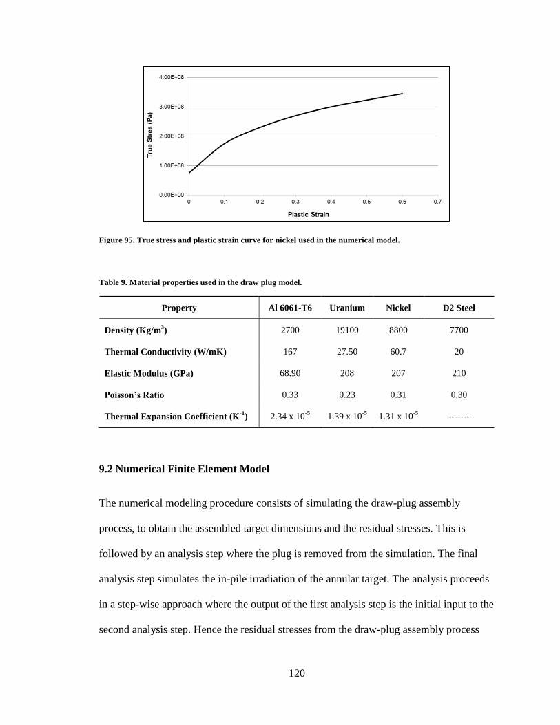
120

Figure 95. True stress and plastic strain curve for nickel used in the numerical model.

Table 9. Material properties used in the draw plug model.

Property Al 6061-T6 Uranium Nickel D2 Steel

Density (Kg/m3) 2700 19100 8800 7700

Thermal Conductivity (W/mK) 167 27.50 60.7 20

Elastic Modulus (GPa) 68.90 208 207 210

Poisson’s Ratio 0.33 0.23 0.31 0.30


) 2.34 x 10-5

1.39 x 10-5

1.31 x 10-5

-------


The numerical modeling procedure consists of simulating the draw-plug assembly

process, to obtain the assembled target dimensions and the residual stresses. This is

followed by an analysis step where the plug is removed from the simulation. The final

analysis step simulates the in-pile irradiation of the annular target. The analysis proceeds

in a step-wise approach where the output of the first analysis step is the initial input to the

second analysis step. Hence the residual stresses from the draw-plug assembly process

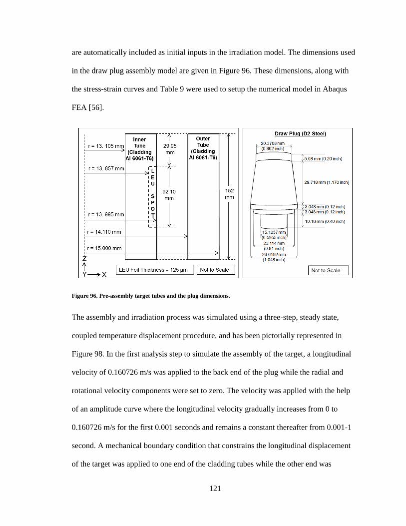
121

are automatically included as initial inputs in the irradiation model. The dimensions used

in the draw plug assembly model are given in Figure 96. These dimensions, along with

the stress-strain curves and Table 9 were used to setup the numerical model in Abaqus

FEA [56].

Figure 96. Pre-assembly target tubes and the plug dimensions.

The assembly and irradiation process was simulated using a three-step, steady state,

coupled temperature displacement procedure, and has been pictorially represented in

Figure 98. In the first analysis step to simulate the assembly of the target, a longitudinal

velocity of 0.160726 m/s was applied to the back end of the plug while the radial and

rotational velocity components were set to zero. The velocity was applied with the help

of an amplitude curve where the longitudinal velocity gradually increases from 0 to

0.160726 m/s for the first 0.001 seconds and remains a constant thereafter from 0.001-1

second. A mechanical boundary condition that constrains the longitudinal displacement

of the target was applied to one end of the cladding tubes while the other end was

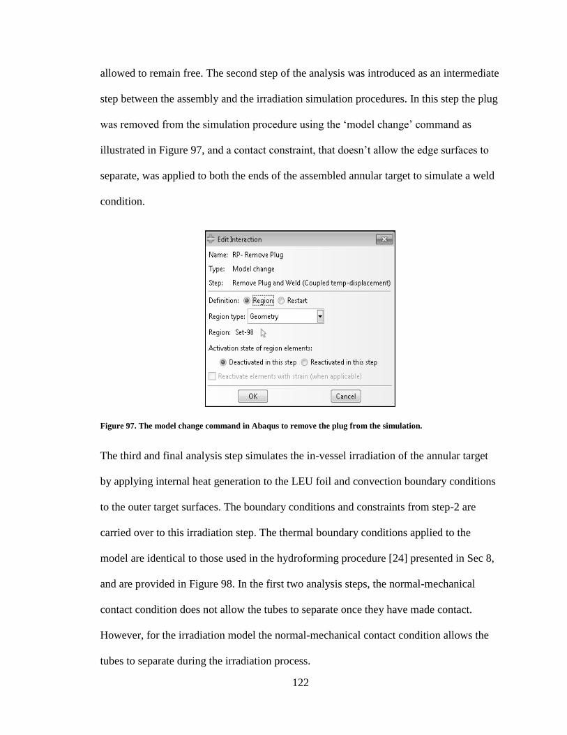
122

allowed to remain free. The second step of the analysis was introduced as an intermediate

step between the assembly and the irradiation simulation procedures. In this step the plug

was removed from the simulation procedure using the ‘model change’ command as

illustrated in Figure 97, and a contact constraint, that doesn’t allow the edge surfaces to

separate, was applied to both the ends of the assembled annular target to simulate a weld

condition.

Figure 97. The model change command in Abaqus to remove the plug from the simulation.

The third and final analysis step simulates the in-vessel irradiation of the annular target

by applying internal heat generation to the LEU foil and convection boundary conditions

to the outer target surfaces. The boundary conditions and constraints from step-2 are

carried over to this irradiation step. The thermal boundary conditions applied to the

model are identical to those used in the hydroforming procedure [24] presented in Sec 8,

and are provided in Figure 98. In the first two analysis steps, the normal-mechanical

contact condition does not allow the tubes to separate once they have made contact.

However, for the irradiation model the normal-mechanical contact condition allows the

tubes to separate during the irradiation process.

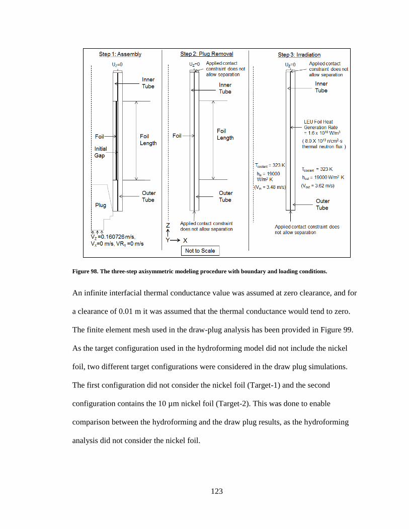
123

Figure 98. The three-step axisymmetric modeling procedure with boundary and loading conditions.

An infinite interfacial thermal conductance value was assumed at zero clearance, and for

a clearance of 0.01 m it was assumed that the thermal conductance would tend to zero.

The finite element mesh used in the draw-plug analysis has been provided in Figure 99.

As the target configuration used in the hydroforming model did not include the nickel

foil, two different target configurations were considered in the draw plug simulations.

The first configuration did not consider the nickel foil (Target-1) and the second

configuration contains the 10 µm nickel foil (Target-2). This was done to enable

comparison between the hydroforming and the draw plug results, as the hydroforming

analysis did not consider the nickel foil.

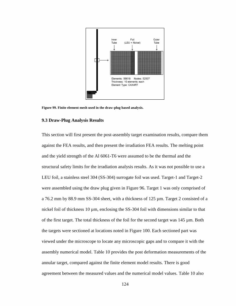
124

Figure 99. Finite element mesh used in the draw-plug based analysis.

9.3 Draw-Plug Analysis Results

This section will first present the post-assembly target examination results, compare them

against the FEA results, and then present the irradiation FEA results. The melting point

and the yield strength of the Al 6061-T6 were assumed to be the thermal and the

structural safety limits for the irradiation analysis results. As it was not possible to use a

LEU foil, a stainless steel 304 (SS-304) surrogate foil was used. Target-1 and Target-2

were assembled using the draw plug given in Figure 96. Target 1 was only comprised of

a 76.2 mm by 88.9 mm SS-304 sheet, with a thickness of 125 µm. Target 2 consisted of a

nickel foil of thickness 10 µm, enclosing the SS-304 foil with dimensions similar to that

of the first target. The total thickness of the foil for the second target was 145 µm. Both

the targets were sectioned at locations noted in Figure 100. Each sectioned part was

viewed under the microscope to locate any microscopic gaps and to compare it with the

assembly numerical model. Table 10 provides the post deformation measurements of the

annular target, compared against the finite element model results. There is good

agreement between the measured values and the numerical model values. Table 10 also

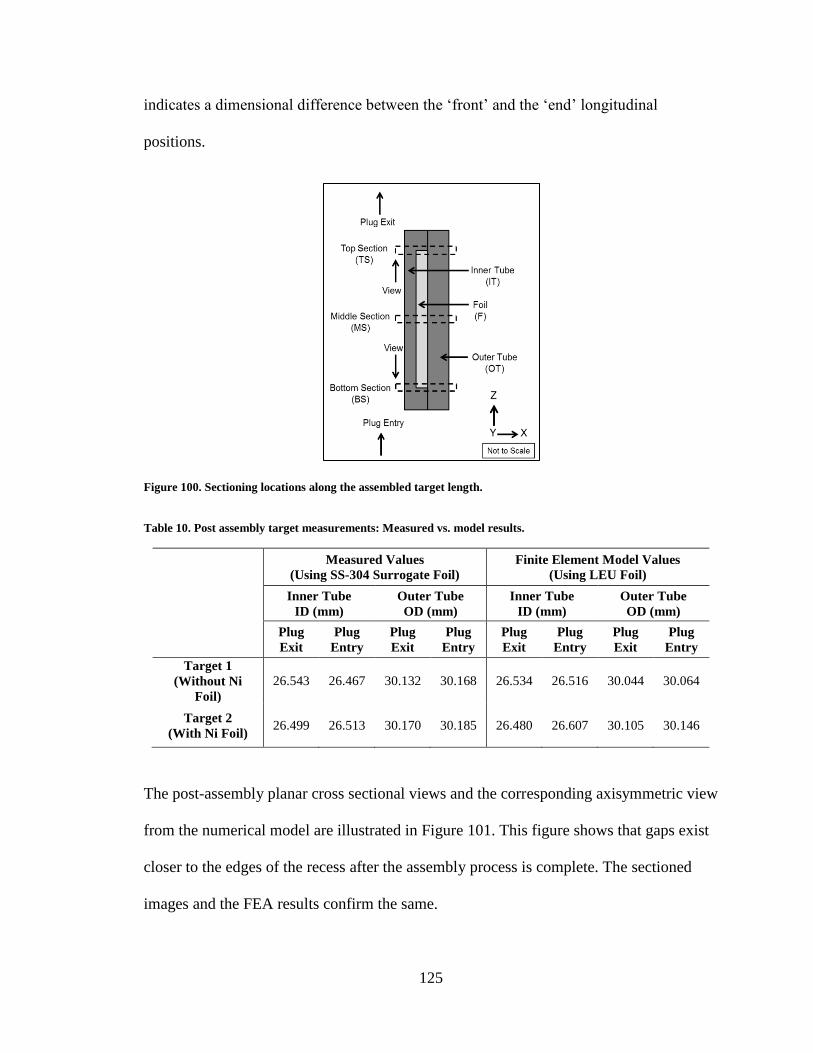
125

indicates a dimensional difference between the ‘front’ and the ‘end’ longitudinal

positions.

Figure 100. Sectioning locations along the assembled target length.

Table 10. Post assembly target measurements: Measured vs. model results.

Measured Values

(Using SS-304 Surrogate Foil)

Finite Element Model Values

(Using LEU Foil)

Inner Tube

ID (mm)

Outer Tube

OD (mm)

Inner Tube

ID (mm)

Outer Tube

OD (mm)

Plug

Exit

Plug

Entry

Plug

Exit

Plug

Entry

Plug

Exit

Plug

Entry

Plug

Exit

Plug

Entry

Target 1

(Without Ni

Foil)

26.543 26.467 30.132 30.168 26.534 26.516 30.044 30.064

Target 2

(With Ni Foil) 26.499 26.513 30.170 30.185 26.480 26.607 30.105 30.146

The post-assembly planar cross sectional views and the corresponding axisymmetric view

from the numerical model are illustrated in Figure 101. This figure shows that gaps exist

closer to the edges of the recess after the assembly process is complete. The sectioned

images and the FEA results confirm the same.

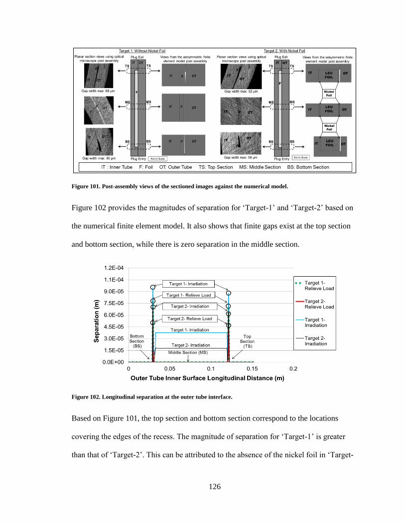
126

Figure 101. Post-assembly views of the sectioned images against the numerical model.

Figure 102 provides the magnitudes of separation for ‘Target-1’ and ‘Target-2’ based on

the numerical finite element model. It also shows that finite gaps exist at the top section

and bottom section, while there is zero separation in the middle section.

Figure 102. Longitudinal separation at the outer tube interface.

Based on Figure 101, the top section and bottom section correspond to the locations

covering the edges of the recess. The magnitude of separation for ‘Target-1’ is greater

than that of ‘Target-2’. This can be attributed to the absence of the nickel foil in ‘Target-

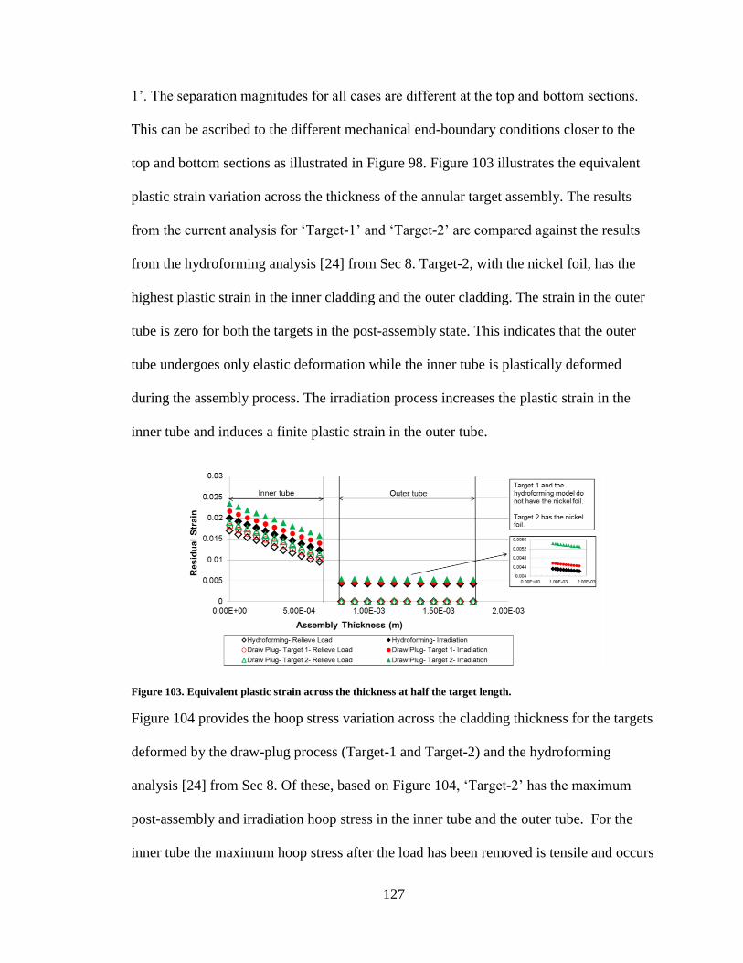
127

1’. The separation magnitudes for all cases are different at the top and bottom sections.

This can be ascribed to the different mechanical end-boundary conditions closer to the

top and bottom sections as illustrated in Figure 98. Figure 103 illustrates the equivalent

plastic strain variation across the thickness of the annular target assembly. The results

from the current analysis for ‘Target-1’ and ‘Target-2’ are compared against the results

from the hydroforming analysis [24] from Sec 8. Target-2, with the nickel foil, has the

highest plastic strain in the inner cladding and the outer cladding. The strain in the outer

tube is zero for both the targets in the post-assembly state. This indicates that the outer

tube undergoes only elastic deformation while the inner tube is plastically deformed

during the assembly process. The irradiation process increases the plastic strain in the

inner tube and induces a finite plastic strain in the outer tube.

Figure 103. Equivalent plastic strain across the thickness at half the target length.

Figure 104 provides the hoop stress variation across the cladding thickness for the targets

deformed by the draw-plug process (Target-1 and Target-2) and the hydroforming

analysis [24] from Sec 8. Of these, based on Figure 104, ‘Target-2’ has the maximum

post-assembly and irradiation hoop stress in the inner tube and the outer tube. For the

inner tube the maximum hoop stress after the load has been removed is tensile and occurs

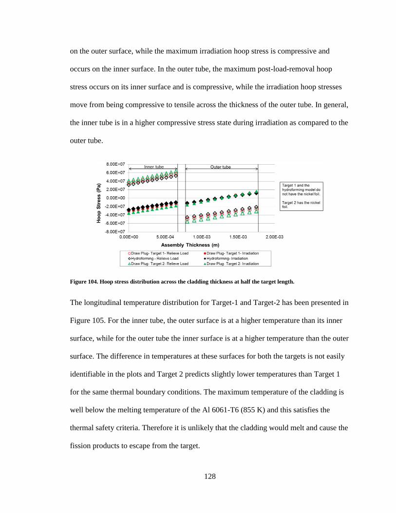
128

on the outer surface, while the maximum irradiation hoop stress is compressive and

occurs on the inner surface. In the outer tube, the maximum post-load-removal hoop

stress occurs on its inner surface and is compressive, while the irradiation hoop stresses

move from being compressive to tensile across the thickness of the outer tube. In general,

the inner tube is in a higher compressive stress state during irradiation as compared to the

outer tube.

Figure 104. Hoop stress distribution across the cladding thickness at half the target length.

The longitudinal temperature distribution for Target-1 and Target-2 has been presented in

Figure 105. For the inner tube, the outer surface is at a higher temperature than its inner

surface, while for the outer tube the inner surface is at a higher temperature than the outer

surface. The difference in temperatures at these surfaces for both the targets is not easily

identifiable in the plots and Target 2 predicts slightly lower temperatures than Target 1

for the same thermal boundary conditions. The maximum temperature of the cladding is

well below the melting temperature of the Al 6061-T6 (855 K) and this satisfies the

thermal safety criteria. Therefore it is unlikely that the cladding would melt and cause the

fission products to escape from the target.

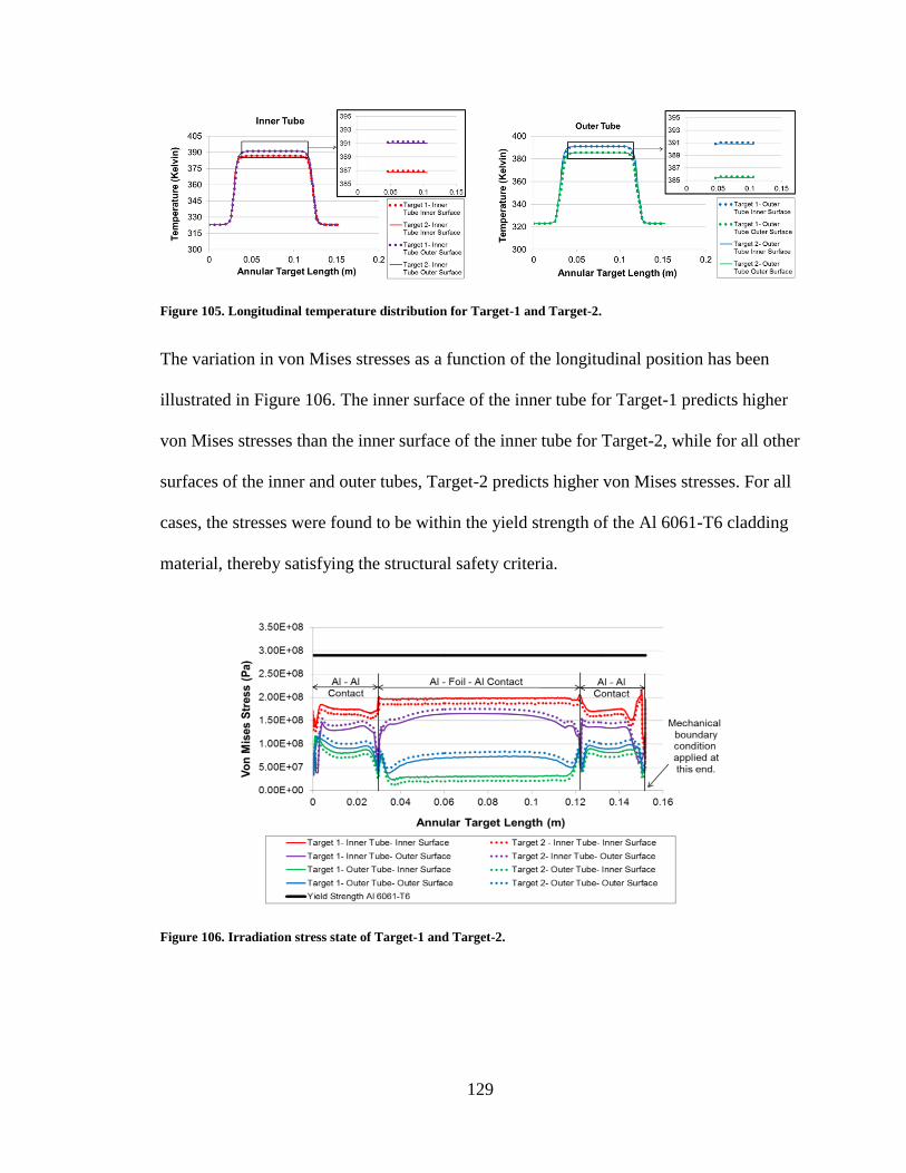
129

Figure 105. Longitudinal temperature distribution for Target-1 and Target-2.

The variation in von Mises stresses as a function of the longitudinal position has been

illustrated in Figure 106. The inner surface of the inner tube for Target-1 predicts higher

von Mises stresses than the inner surface of the inner tube for Target-2, while for all other

surfaces of the inner and outer tubes, Target-2 predicts higher von Mises stresses. For all

cases, the stresses were found to be within the yield strength of the Al 6061-T6 cladding

material, thereby satisfying the structural safety criteria.

Figure 106. Irradiation stress state of Target-1 and Target-2.

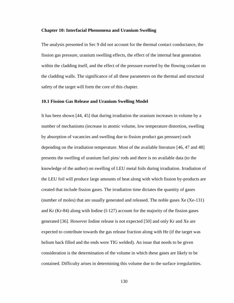
130

Chapter 10: Interfacial Phenomena and Uranium Swelling

The analysis presented in Sec 9 did not account for the thermal contact conductance, the

fission gas pressure, uranium swelling effects, the effect of the internal heat generation

within the cladding itself, and the effect of the pressure exerted by the flowing coolant on

the cladding walls. The significance of all these parameters on the thermal and structural

safety of the target will form the core of this chapter.

10.1 Fission Gas Release and Uranium Swelling Model

It has been shown [44, 45] that during irradiation the uranium increases in volume by a

number of mechanisms (increase in atomic volume, low temperature distortion, swelling

by absorption of vacancies and swelling due to fission product gas pressure) each

depending on the irradiation temperature. Most of the available literature [46, 47 and 48]

presents the swelling of uranium fuel pins/ rods and there is no available data (to the

knowledge of the author) on swelling of LEU metal foils during irradiation. Irradiation of

the LEU foil will produce large amounts of heat along with which fission by-products are

created that include fission gases. The irradiation time dictates the quantity of gases

(number of moles) that are usually generated and released. The noble gases Xe (Xe-131)

and Kr (Kr-84) along with Iodine (I-127) account for the majority of the fission gases

generated [36]. However Iodine release is not expected [50] and only Kr and Xe are

expected to contribute towards the gas release fraction along with He (if the target was

helium back filled and the ends were TIG welded). An issue that needs to be given

consideration is the determination of the volume in which these gases are likely to be

contained. Difficulty arises in determining this volume due to the surface irregularities.

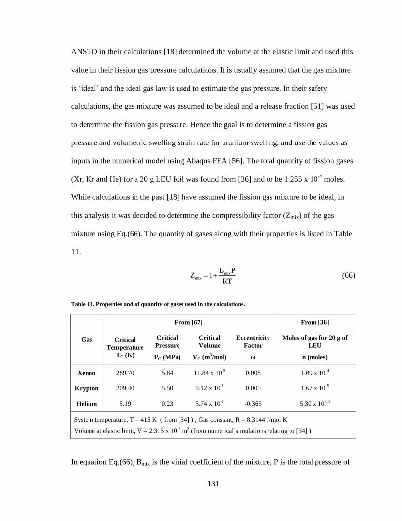
131

ANSTO in their calculations [18] determined the volume at the elastic limit and used this

value in their fission gas pressure calculations. It is usually assumed that the gas mixture

is ‘ideal’ and the ideal gas law is used to estimate the gas pressure. In their safety

calculations, the gas mixture was assumed to be ideal and a release fraction [51] was used

to determine the fission gas pressure. Hence the goal is to determine a fission gas

pressure and volumetric swelling strain rate for uranium swelling, and use the values as

inputs in the numerical model using Abaqus FEA [56]. The total quantity of fission gases

(Xr, Kr and He) for a 20 g LEU foil was found from [36] and to be 1.255 x 10-4

moles.

While calculations in the past [18] have assumed the fission gas mixture to be ideal, in

this analysis it was decided to determine the compressibility factor (Zmix) of the gas

mixture using Eq.(66). The quantity of gases along with their properties is listed in Table

11.

mixmix

B PZ 1

RT (66)

Table 11. Properties and of quantity of gases used in the calculations.

Gas

From [67] From [36]

Critical

Temperature

TC (K)

Critical

Pressure

PC (MPa)

Critical

Volume

VC (m3/mol)

Eccentricity

Factor

ω

Moles of gas for 20 g of

LEU

n (moles)

Xenon 289.70 5.84 11.84 x 10-5

0.008 1.09 x 10-4

Krypton 209.40 5.50 9.12 x 10-5

0.005 1.67 x 10-5

Helium 5.19 0.23 5.74 x 10-5

-0.365 5.30 x 10-11

System temperature, T = 415 K ( from [34] ) ; Gas constant, R = 8.3144 J/mol K

Volume at elastic limit, V = 2.315 x 10-7

m3 (from numerical simulations relating to [34] )

In equation Eq.(66), Bmix is the virial coefficient of the mixture, P is the total pressure of

132

the mixture, R is the ideal gas constant, and T is the system temperature. The current

approach to determine the compressibility factor and the fission gas pressure was

obtained from [67]. The first part of the calculation is to estimate all the individual virial

coefficients, Bi, using Eq. (67). The critical compressibility factor, Zci, for each

component (i=He, Xe, Kr) can be calculated using Eq.(68).

i

i1.6 4.2

C,i

C,i C,

i

i

C,B P 0.422 0.1720.083 0.139

RT T T

T T

(67)

i C,i i

C,i

C,i C,i

B B1 1

R

P

VTZ (68)

Since the fission gas mixture in this analysis consists of three components, the mixing

rule for a two component interaction is extended. The formulas that apply to a two

component interaction to determine the critical temperature, critical compressibility

factor, critical volume, eccentricity factor, critical pressure and temperature, are given by

Eqs. (69)-(72) respectively. The subscripts ‘i’ and ‘j’ individually refer to any of the three

gases (Xe, Kr, He).

C,ij C,i C, jT T T (69)

C,i C, j

C,ij

Z ZZ

2

(70)

31/3 1/3

C,i C, j

C,ij

V VV

2

(71)

133

i j

ij

C,ij C,ij

C,ij

C,ij

2

Z RTP

V

(72)

The second virial coefficient, which accounts for the interactions between a component

pair can be determined using Eq.(73). With the knowledge of all the second virial

coefficients and the individual component mole fractions (yi or yj) the virial coefficient of

the mixture (Bmix) can be determined using Eq.(74). Once Bmix has been determined, the

gas mixture compressibility factor can be found using Eq.(66).

ij C,ij

ij1.6 4.2

C,ij

C,ij C,ij

B P 0.422 0.1720.083 0.139

RT T T

T T

(73)

mix i j ij

i j

ij ji

B y y B

B B

(74)

The compressibility factor, using the above equations and the information provided in

Table 11, was found to be 0.83 implying that the gas mixture is non-ideal. Hence the gas

pressure can be determined using Eq.(75). Using Table 11 and Eq.(75), the gas pressure

was found to be 1.59 MPa.

mix total

elastic limit

Z *n *R *TP

V (75)

This pressure of 1.59 MPa corresponds to a 100 % gas release situation. However, a 100

% gas release situation is unrealistic and typically lesser than 1 % of the generated gas is

134

released from the foil by the mechanism of recoil [68, 69]. It has been shown in literature

[51] that this recoil depth can be taken as 5 µm and a factor of 0.25 [70] be used to

account for the gas atoms that fail to make contact with the surface. Using the LEU foil

thickness of 125 µm, taking into consideration the recoil factor of 0.25, a recoil depth of

5 µm and multiplying by a factor of two to account for two sides of the foil, the gas

pressure was determined to be 47.74 kPa using Eq.(76).

interfacial

recoildepthP P 2* *(1 recoil factor)

foil thickness

(76)

Uranium swelling is the increase in volume of uranium during irradiation without

undergoing any change in shape. The noble fission gases (Xe and Kr) precipitate into

small gas bubbles due to their insolubility. A macroscopic increase of these gas bubbles

occurs with increasing temperature and the uranium tends to swell as a result. It is

expected that most of the gases are contained inside the bubbles, and remain constrained

by the surface tension of the metal. The surface tension effects are usually neglected in

the swelling calculations unless the bubble sizes are small [44].

Factors such as the composition of the specimen, irradiation temperature, fission rate and

external restraint have been reported [48] to influence the swelling of uranium. The

majority of the available swelling data in literature, to the author’s knowledge, are

correlations for U-Mo monolithic fuel, with little available data for swelling of low-

enriched uranium foils. Hence, the correlations for a U-Mo fuel will be used to determine

the swelling percentage and the corresponding volumetric strain rate. Work done by [71]

showed that the overall fuel swelling measured by the post irradiation dimensions is a

function of the fission density, and provided an empirical correlation for the percentage

135

volumetric swelling strain as a function of fission density for temperatures below 523 K.

This correlation has been provided by Eq.(77). For an irradiation time of 150 hours,

thermal power ~ 15 kW, and assuming that a single atom of U-235 releases 3.2 x 10-11

J

of energy, the number of fissions was calculated to be 2.36 x 1020

. For an LEU foil of

thickness 125 µm, length 92.10 mm and width 76.2 mm, the fission density was

calculated to be 0.27 x 1027

fissions/m3. Applying this to Eq.(77), the volumetric swelling

strain was calculated to be 1.35 %. The volumetric swelling strain rate was calculated

using Eq.(78) to be 2.48 x 10-8

s-1

.

d0 overall

27d 3

0 overall

27d 3

V5f

V

fissionsfor f 3x10 and T 523K

m

V is the volumetric swelling strain in [%]

V

fissionsf is the fission density in 10 [ ]

m

(77)

0 overall

irradiation

V

Vln 1

100

Volumetric swelling strain rate = Time

(78)

An alternate approach to assess the significance of volumetric swelling would be to

estimate the temperature levels in the target and compare against a swelling versus

temperature curve for uranium. The temperature dependence of swelling in uranium

metal from [49] has been provided in Figure 107. The swelling data from [49] presented

in Figure 107, along with data from [44], indicates significant swelling at temperatures in

excess of 673 K (400 ᵒC) and small to no swelling at temperatures below 623 K (350

ᵒC).

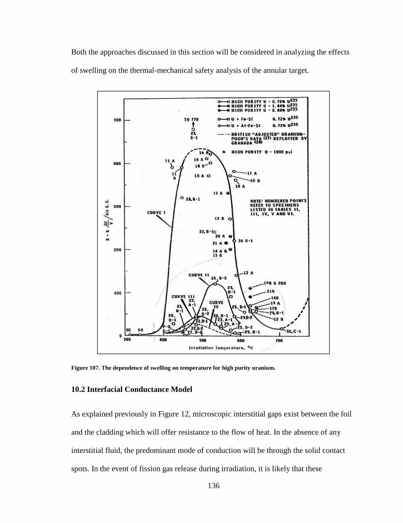
136

Both the approaches discussed in this section will be considered in analyzing the effects

of swelling on the thermal-mechanical safety analysis of the annular target.

Figure 107. The dependence of swelling on temperature for high purity uranium.

10.2 Interfacial Conductance Model

As explained previously in Figure 12, microscopic interstitial gaps exist between the foil

and the cladding which will offer resistance to the flow of heat. In the absence of any

interstitial fluid, the predominant mode of conduction will be through the solid contact

spots. In the event of fission gas release during irradiation, it is likely that these

137

interstitial gaps are filled mostly with a mixture of Xe (Xe-131), Kr (Kr-84), and He

(Helium). Hence the thermal conductivity of the gas in the interstices will depend on the

quantity of this gas mixture which can be obtained from neutronics calculations. It should

be noted that the quantity of fission gases will depend on the reactor, the neutron flux,

irradiation time and burn up. Calculation of the solid spot conductance will require

knowledge of the surface parameters asperity slope, surface roughness apart from the

material properties such as the harmonic average thermal conductivity, hardness of the

softer material.

The total conductance can be expressed as in Eq.(3), with the solid spot conductance

being expressed as a function of the contact pressure and the gap conductance being

expressed as a function of the interface thickness. The goal here is to develop an

expression for the total conductance as a function of the contact pressure and the

interfacial gap. To account for the temperature drop across the interfaces, a thermal

contact conductance model was setup and included in the analysis. The presence of the

nickel foil necessitates the calculation of the contact conductance at the aluminum 6061

T6 - nickel and nickel-uranium interfaces. The aluminum 6061 T6- aluminum 6061 T6

contact conductance model has been provided for reference. Due to the composite target

structure, interfaces exist between the parts in contact. Discontinuities exist at these

interfaces due to microscopic (surface roughness) and macroscopic (waviness)

irregularities on the surfaces of the parts in contact. This results in the formation of solid

contact spots and gas gaps. At the interface of the two surfaces in contact, the expressions

for the harmonic average thermal conductivity (keff), effective modulus of elasticity (E),

combined surface roughness (σcombined) and the effective asperity slope (tanϕ), from [10],

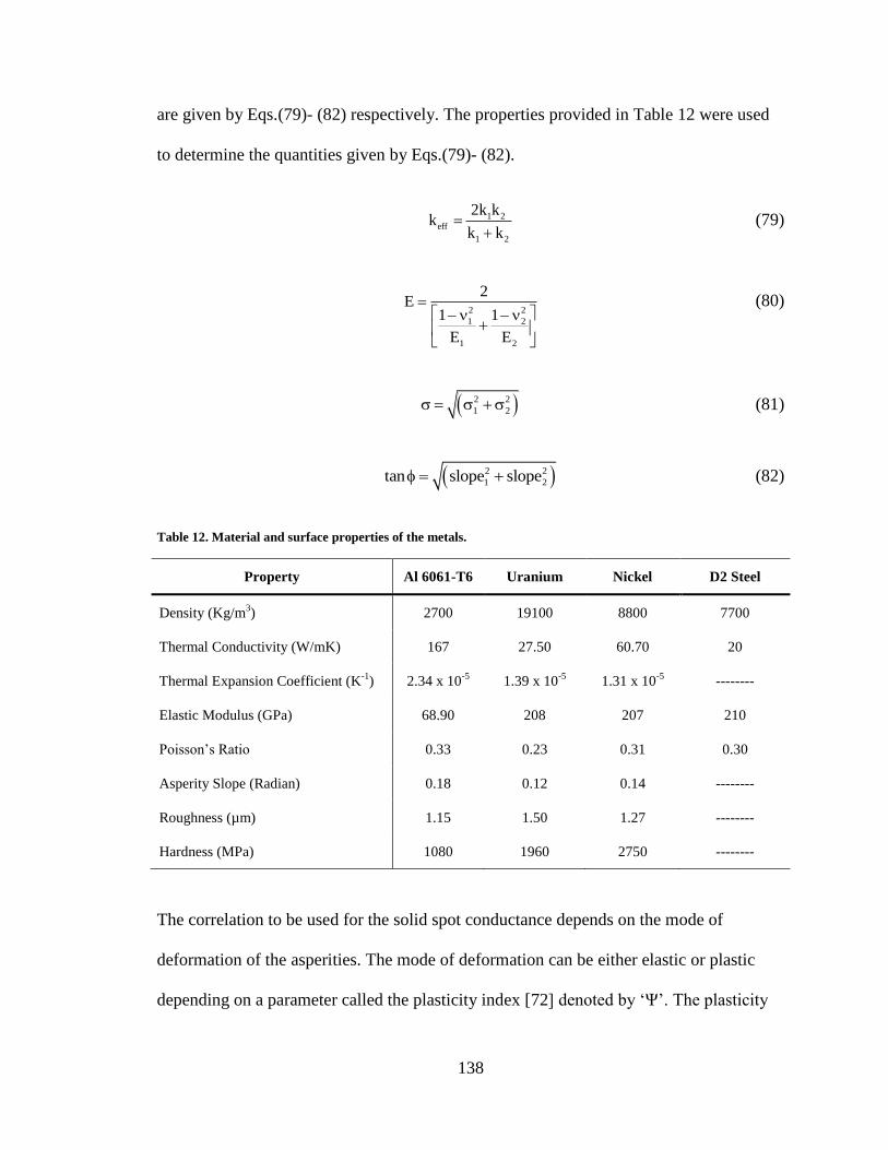
138

are given by Eqs.(79)- (82) respectively. The properties provided in Table 12 were used

to determine the quantities given by Eqs.(79)- (82).

1 2eff

1 2

2k kk

k k

(79)

2 2

1 2

1 2

2E

1 1

E E

(80)

2 2

1 2 (81)

2 2

1 2tan slope slope (82)

Table 12. Material and surface properties of the metals.

Property Al 6061-T6 Uranium Nickel D2 Steel

Density (Kg/m3) 2700 19100 8800 7700

Thermal Conductivity (W/mK) 167 27.50 60.70 20


) 2.34 x 10-5

1.39 x 10-5

1.31 x 10-5

--------


Poisson’s Ratio 0.33 0.23 0.31 0.30

Asperity Slope (Radian) 0.18 0.12 0.14 --------

Roughness (µm) 1.15 1.50 1.27 --------

Hardness (MPa) 1080 1960 2750 --------

The correlation to be used for the solid spot conductance depends on the mode of

deformation of the asperities. The mode of deformation can be either elastic or plastic

depending on a parameter called the plasticity index [72] denoted by ‘Ψ’. The plasticity

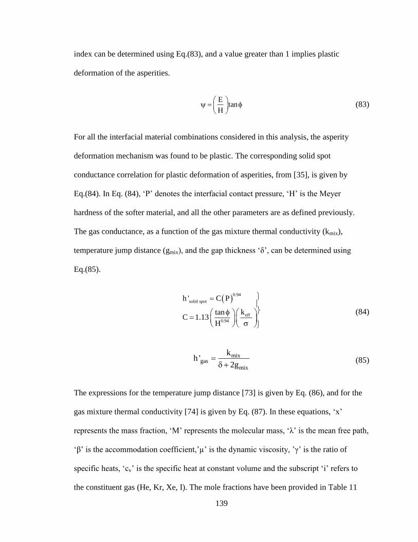
139

index can be determined using Eq.(83), and a value greater than 1 implies plastic

deformation of the asperities.

E

tanH

(83)

For all the interfacial material combinations considered in this analysis, the asperity

deformation mechanism was found to be plastic. The corresponding solid spot

conductance correlation for plastic deformation of asperities, from [35], is given by

Eq.(84). In Eq. (84), ‘P’ denotes the interfacial contact pressure, ‘H’ is the Meyer

hardness of the softer material, and all the other parameters are as defined previously.

The gas conductance, as a function of the gas mixture thermal conductivity (kmix),

temperature jump distance (gmix), and the gap thickness ‘δ’, can be determined using

Eq.(85).

0.94

solid spot

eff

0.94

h ' C P

ktanC 1.13

H

(84)

mix

gasmix

kh '

2g

(85)

The expressions for the temperature jump distance [73] is given by Eq. (86), and for the

gas mixture thermal conductivity [74] is given by Eq. (87). In these equations, ‘x’

represents the mass fraction, ‘M’ represents the molecular mass, ‘λ’ is the mean free path,

‘β’ is the accommodation coefficient,’µ’ is the dynamic viscosity, ’γ’ is the ratio of

specific heats, ‘cv’ is the specific heat at constant volume and the subscript ‘i’ refers to

the constituent gas (He, Kr, Xe, I). The mole fractions have been provided in Table 11

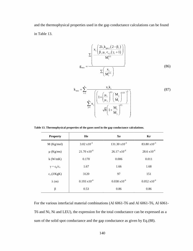
140

and the thermophysical properties used in the gap conductance calculations can be found

in Table 13.

i gas,i i

i

i i v,i i

0.5

i

mix

i

0.5

i

2 k 2x

c 1

M

gx

M

(86)

n

i imix 2

0.5 0.25i 1

ji

n j i

j 0.5j 1

i

j

x kk

M1

Mx

M8 1

M

(87)

Table 13. Thermophysical properties of the gases used in the gap conductance calculations.

Property He Xe Kr

M (Kg/mol) 3.02 x10-3

131.30 x10-3

83.80 x10-3

µ (Kg/ms) 21.70 x10-6

26.17 x10-6

28.6 x10-6

k (W/mK) 0.170 0.006 0.011

γ = cp/cv 1.67 1.66 1.68

cv (J/KgK) 3120 97 151

λ (m) 0.193 x10-6

0.038 x10-6

0.052 x10-6

β 0.53 0.86 0.86

For the various interfacial material combinations (Al 6061-T6 and Al 6061-T6, Al 6061-

T6 and Ni, Ni and LEU), the expression for the total conductance can be expressed as a

sum of the solid spot conductance and the gap conductance as given by Eq.(88).

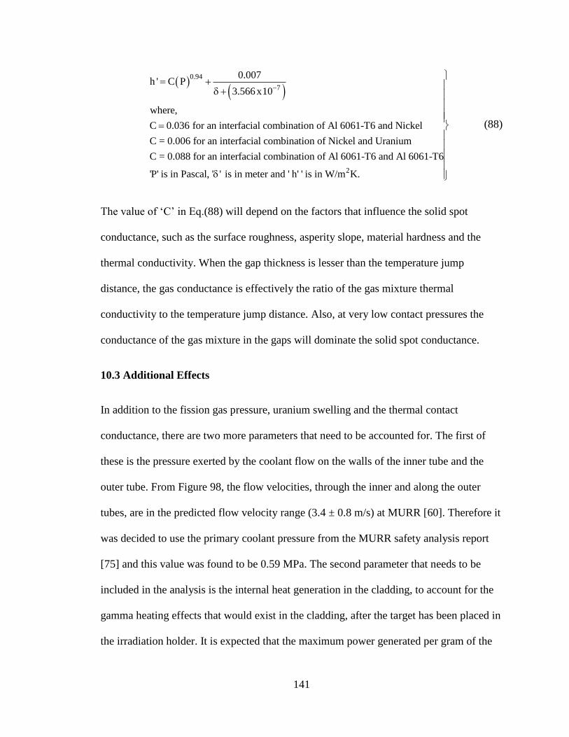
141

0.94

7

0.007h ' C P

3.566 x10

where,

C 0.036 for an interfacial combination of Al 6061-T6 and Nickel

C = 0.006 for an interfacial combination of Nickel and Uranium

C = 0.088 for an interfacial combination

2

of Al 6061-T6 and Al 6061-T6

'P' is in Pascal, ' ' is in meter and ' h' ' is in W/m K.

(88)

The value of ‘C’ in Eq.(88) will depend on the factors that influence the solid spot

conductance, such as the surface roughness, asperity slope, material hardness and the

thermal conductivity. When the gap thickness is lesser than the temperature jump

distance, the gas conductance is effectively the ratio of the gas mixture thermal

conductivity to the temperature jump distance. Also, at very low contact pressures the

conductance of the gas mixture in the gaps will dominate the solid spot conductance.

10.3 Additional Effects

In addition to the fission gas pressure, uranium swelling and the thermal contact

conductance, there are two more parameters that need to be accounted for. The first of

these is the pressure exerted by the coolant flow on the walls of the inner tube and the

outer tube. From Figure 98, the flow velocities, through the inner and along the outer

tubes, are in the predicted flow velocity range (3.4 ± 0.8 m/s) at MURR [60]. Therefore it

was decided to use the primary coolant pressure from the MURR safety analysis report

[75] and this value was found to be 0.59 MPa. The second parameter that needs to be

included in the analysis is the internal heat generation in the cladding, to account for the

gamma heating effects that would exist in the cladding, after the target has been placed in

the irradiation holder. It is expected that the maximum power generated per gram of the

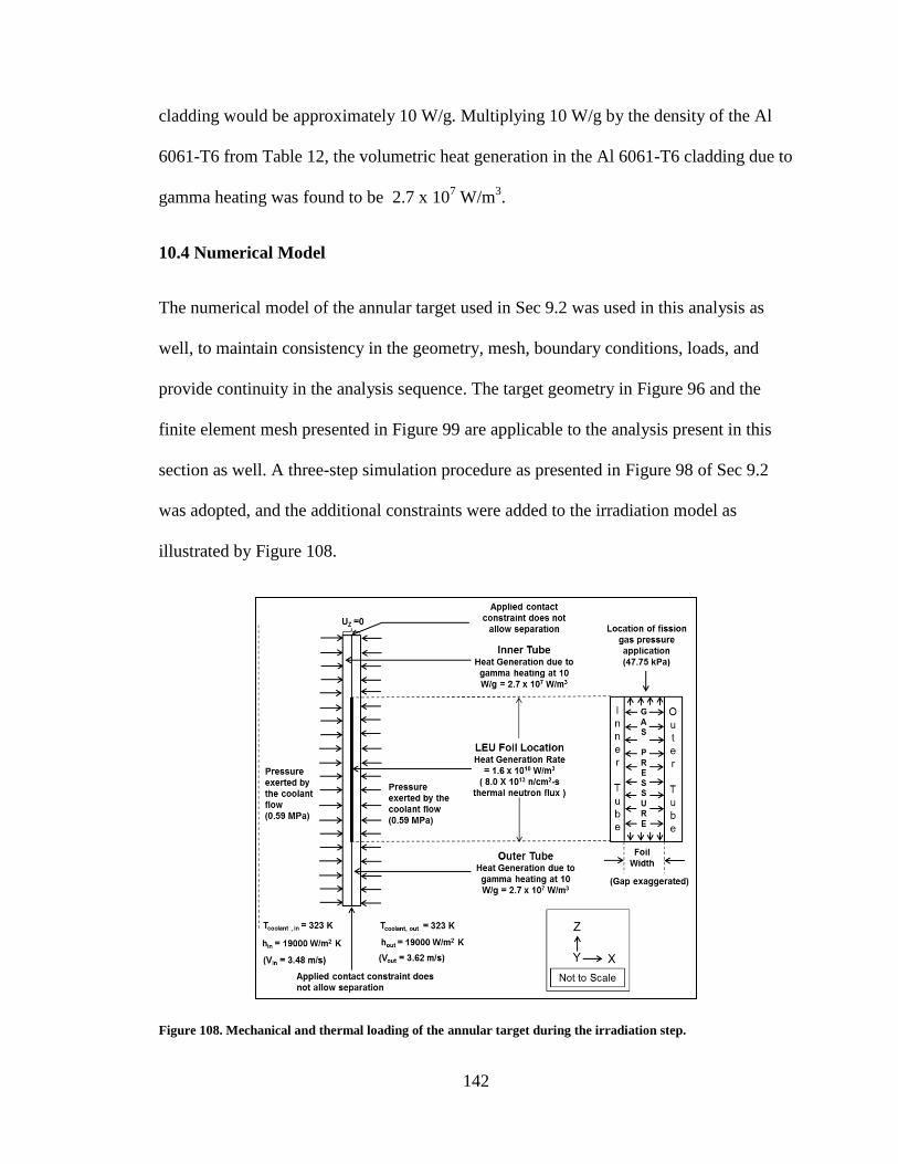
142

cladding would be approximately 10 W/g. Multiplying 10 W/g by the density of the Al

6061-T6 from Table 12, the volumetric heat generation in the Al 6061-T6 cladding due to

gamma heating was found to be 2.7 x 107 W/m

3.

10.4 Numerical Model

The numerical model of the annular target used in Sec 9.2 was used in this analysis as

well, to maintain consistency in the geometry, mesh, boundary conditions, loads, and

provide continuity in the analysis sequence. The target geometry in Figure 96 and the

finite element mesh presented in Figure 99 are applicable to the analysis present in this

section as well. A three-step simulation procedure as presented in Figure 98 of Sec 9.2

was adopted, and the additional constraints were added to the irradiation model as

illustrated by Figure 108.

Figure 108. Mechanical and thermal loading of the annular target during the irradiation step.

143

The developed thermal conductance model given by Eq. (88) was input into Abaqus FEA

[56] and applied to the appropriate interfaces. The normal and tangential mechanical

contact definitions were kept the same as in Sec 9.2. The calculated fission gas pressure

of 47.75 kPa (based on fractional gas release) was applied as a pressure loading condition

to the surfaces of the inner and outer tubes as illustrated in Figure 108. The calculated

volumetric swelling strain rate of 2.48 x 10-8

s-1

was included under the plastic material

property definition for uranium as illustrated in Figure 109.

Figure 109. Volumetric swelling strain rate definition location.

10.5 Results

The results will focus on the von Mises stresses and the temperature distribution in the

cladding, and provide comparisons against the yield strength and the melting point of the

Al 6061-T6. The various applied constraints have been split into 5 cases, as shown in

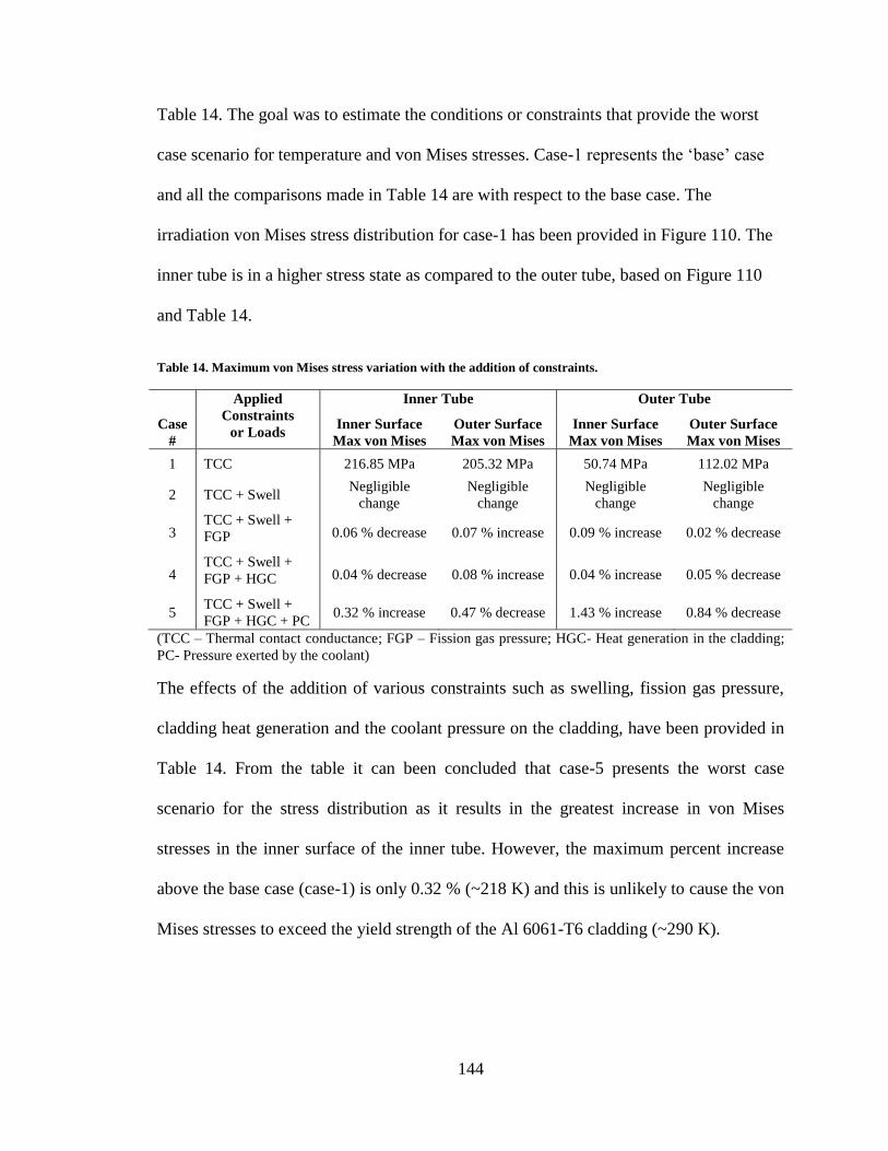
144

Table 14. The goal was to estimate the conditions or constraints that provide the worst

case scenario for temperature and von Mises stresses. Case-1 represents the ‘base’ case

and all the comparisons made in Table 14 are with respect to the base case. The

irradiation von Mises stress distribution for case-1 has been provided in Figure 110. The

inner tube is in a higher stress state as compared to the outer tube, based on Figure 110

and Table 14.

Table 14. Maximum von Mises stress variation with the addition of constraints.

Applied

Constraints

or Loads

Inner Tube Outer Tube

Case

#

Inner Surface

Max von Mises

Outer Surface

Max von Mises

Inner Surface

Max von Mises

Outer Surface

Max von Mises

1 TCC 216.85 MPa 205.32 MPa 50.74 MPa 112.02 MPa

2 TCC + Swell Negligible

change

Negligible

change

Negligible

change

Negligible

change

3 TCC + Swell +

FGP 0.06 % decrease 0.07 % increase 0.09 % increase 0.02 % decrease

4 TCC + Swell +

FGP + HGC 0.04 % decrease 0.08 % increase 0.04 % increase 0.05 % decrease

5 TCC + Swell +

FGP + HGC + PC 0.32 % increase 0.47 % decrease 1.43 % increase 0.84 % decrease

(TCC – Thermal contact conductance; FGP – Fission gas pressure; HGC- Heat generation in the cladding;

PC- Pressure exerted by the coolant)

The effects of the addition of various constraints such as swelling, fission gas pressure,

cladding heat generation and the coolant pressure on the cladding, have been provided in

Table 14. From the table it can been concluded that case-5 presents the worst case

scenario for the stress distribution as it results in the greatest increase in von Mises

stresses in the inner surface of the inner tube. However, the maximum percent increase

above the base case (case-1) is only 0.32 % (~218 K) and this is unlikely to cause the von

Mises stresses to exceed the yield strength of the Al 6061-T6 cladding (~290 K).

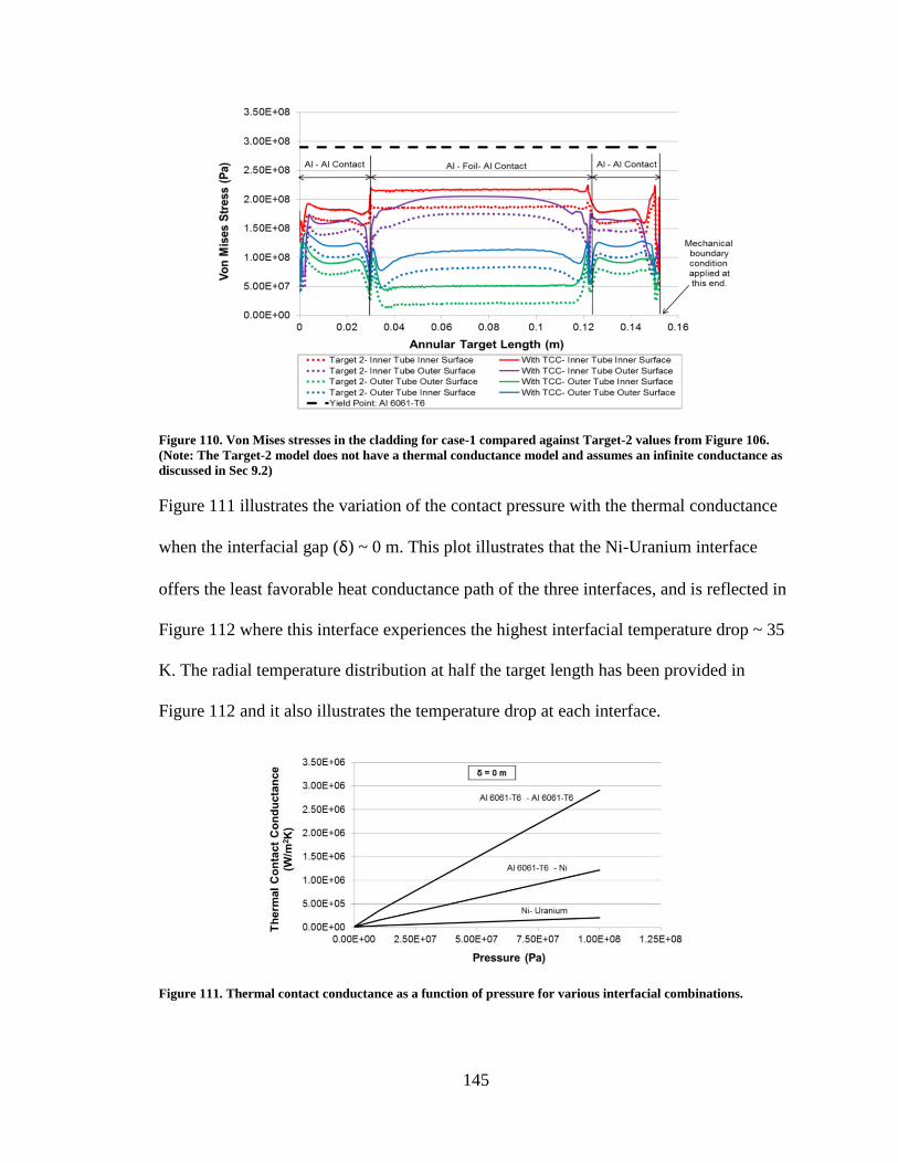
145

Figure 110. Von Mises stresses in the cladding for case-1 compared against Target-2 values from Figure 106.

(Note: The Target-2 model does not have a thermal conductance model and assumes an infinite conductance as

discussed in Sec 9.2)

Figure 111 illustrates the variation of the contact pressure with the thermal conductance

when the interfacial gap (δ) ~ 0 m. This plot illustrates that the Ni-Uranium interface

offers the least favorable heat conductance path of the three interfaces, and is reflected in

Figure 112 where this interface experiences the highest interfacial temperature drop ~ 35

K. The radial temperature distribution at half the target length has been provided in

Figure 112 and it also illustrates the temperature drop at each interface.

Figure 111. Thermal contact conductance as a function of pressure for various interfacial combinations.

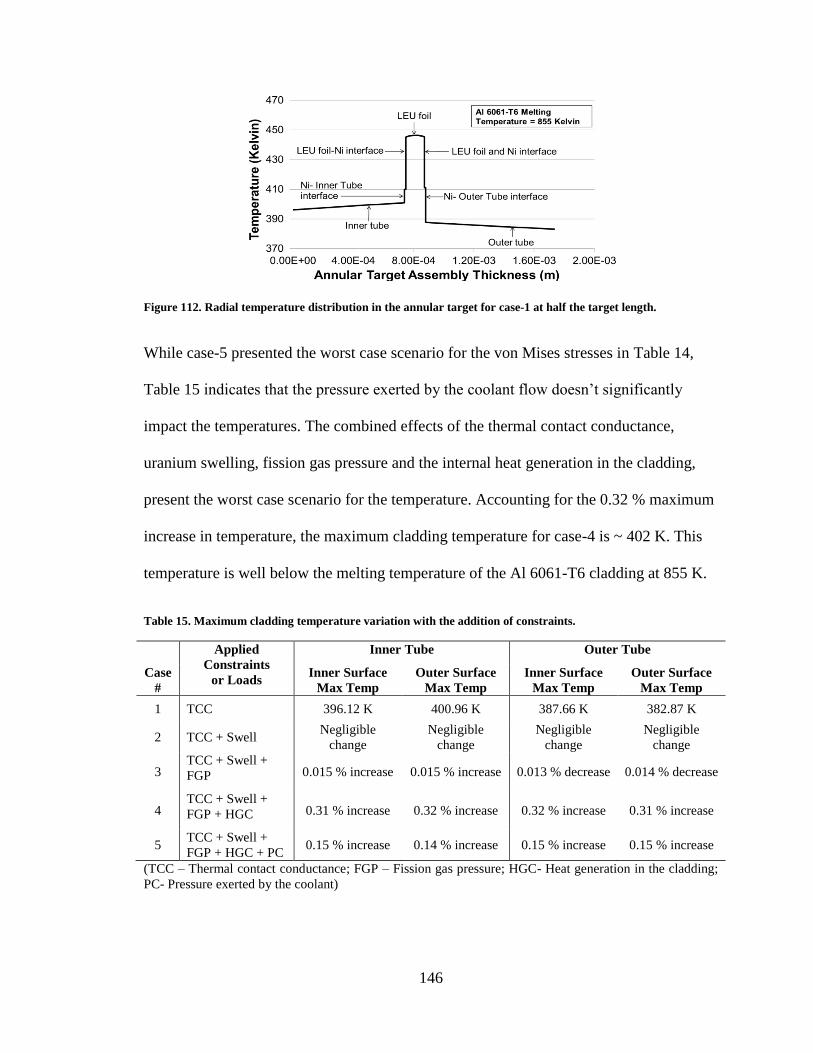
146

Figure 112. Radial temperature distribution in the annular target for case-1 at half the target length.

While case-5 presented the worst case scenario for the von Mises stresses in Table 14,

Table 15 indicates that the pressure exerted by the coolant flow doesn’t significantly

impact the temperatures. The combined effects of the thermal contact conductance,

uranium swelling, fission gas pressure and the internal heat generation in the cladding,

present the worst case scenario for the temperature. Accounting for the 0.32 % maximum

increase in temperature, the maximum cladding temperature for case-4 is ~ 402 K. This

temperature is well below the melting temperature of the Al 6061-T6 cladding at 855 K.

Table 15. Maximum cladding temperature variation with the addition of constraints.

Applied

Constraints

or Loads

Inner Tube Outer Tube

Case

#

Inner Surface

Max Temp

Outer Surface

Max Temp

Inner Surface

Max Temp

Outer Surface

Max Temp

1 TCC 396.12 K 400.96 K 387.66 K 382.87 K

2 TCC + Swell Negligible

change

Negligible

change

Negligible

change

Negligible

change

3 TCC + Swell +

FGP 0.015 % increase 0.015 % increase 0.013 % decrease 0.014 % decrease

4 TCC + Swell +

FGP + HGC 0.31 % increase 0.32 % increase 0.32 % increase 0.31 % increase

5 TCC + Swell +

FGP + HGC + PC 0.15 % increase 0.14 % increase 0.15 % increase 0.15 % increase

(TCC – Thermal contact conductance; FGP – Fission gas pressure; HGC- Heat generation in the cladding;

PC- Pressure exerted by the coolant)

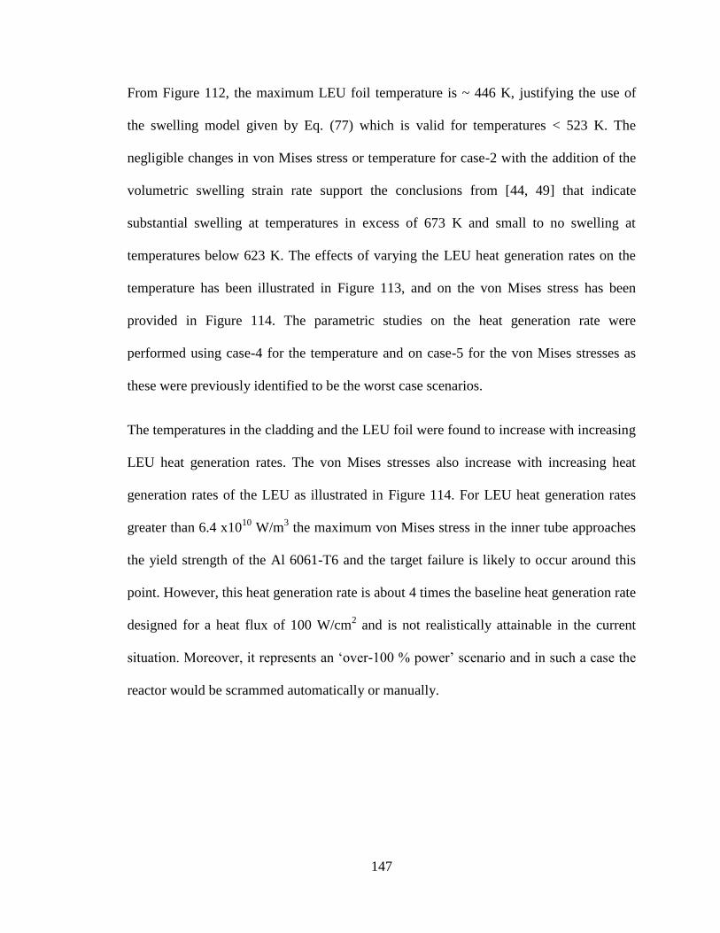
147

From Figure 112, the maximum LEU foil temperature is ~ 446 K, justifying the use of

the swelling model given by Eq. (77) which is valid for temperatures < 523 K. The

negligible changes in von Mises stress or temperature for case-2 with the addition of the

volumetric swelling strain rate support the conclusions from [44, 49] that indicate

substantial swelling at temperatures in excess of 673 K and small to no swelling at

temperatures below 623 K. The effects of varying the LEU heat generation rates on the

temperature has been illustrated in Figure 113, and on the von Mises stress has been

provided in Figure 114. The parametric studies on the heat generation rate were

performed using case-4 for the temperature and on case-5 for the von Mises stresses as

these were previously identified to be the worst case scenarios.

The temperatures in the cladding and the LEU foil were found to increase with increasing

LEU heat generation rates. The von Mises stresses also increase with increasing heat

generation rates of the LEU as illustrated in Figure 114. For LEU heat generation rates

greater than 6.4 x1010

W/m3 the maximum von Mises stress in the inner tube approaches

the yield strength of the Al 6061-T6 and the target failure is likely to occur around this

point. However, this heat generation rate is about 4 times the baseline heat generation rate

designed for a heat flux of 100 W/cm2 and is not realistically attainable in the current

situation. Moreover, it represents an ‘over-100 % power’ scenario and in such a case the

reactor would be scrammed automatically or manually.

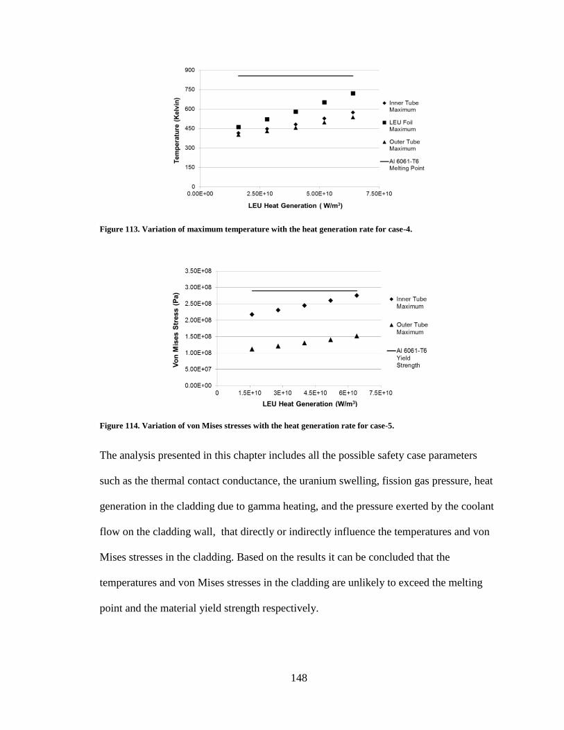
148

Figure 113. Variation of maximum temperature with the heat generation rate for case-4.

Figure 114. Variation of von Mises stresses with the heat generation rate for case-5.

The analysis presented in this chapter includes all the possible safety case parameters

such as the thermal contact conductance, the uranium swelling, fission gas pressure, heat

generation in the cladding due to gamma heating, and the pressure exerted by the coolant

flow on the cladding wall, that directly or indirectly influence the temperatures and von

Mises stresses in the cladding. Based on the results it can be concluded that the

temperatures and von Mises stresses in the cladding are unlikely to exceed the melting

point and the material yield strength respectively.

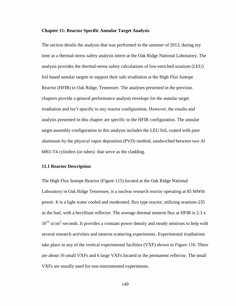
149

Chapter 11: Reactor Specific Annular Target Analysis

The section details the analysis that was performed in the summer of 2013, during my

time as a thermal-stress safety analysis intern at the Oak Ridge National Laboratory. The

analysis provides the thermal-stress safety calculations of low-enriched uranium (LEU)

foil based annular targets to support their safe irradiation at the High Flux Isotope

Reactor (HFIR) in Oak Ridge, Tennessee. The analyses presented in the previous

chapters provide a general performance analysis envelope for the annular target

irradiation and isn’t specific to any reactor configuration. However, the results and

analysis presented in this chapter are specific to the HFIR configuration. The annular

target assembly configuration in this analysis includes the LEU foil, coated with pure

aluminum by the physical vapor deposition (PVD) method, sandwiched between two Al

6061-T4 cylinders (or tubes) that serve as the cladding.

11.1 Reactor Description

The High Flux Isotope Reactor (Figure 115) located at the Oak Ridge National

Laboratory in Oak Ridge Tennessee, is a nuclear research reactor operating at 85 MWth

power. It is a light water cooled and moderated, flux type reactor, utilizing uranium-235

as the fuel, with a beryllium reflector. The average thermal neutron flux at HFIR is 2.3 x

1015

n/cm2-seconds. It provides a constant power density and steady neutrons to help with

several research activities and neutron scattering experiments. Experimental irradiations

take place in any of the vertical experimental facilities (VXF) shown in Figure 116. There

are about 16 small VXFs and 6 large VXFs located in the permanent reflector. The small

VXFs are usually used for non-instrumented experiments.

150

Figure 115. Aerial view of the HFIR facility. (SOURCE: http://energyfromthorium.com/wp-

content/uploads/2012/06/ORNL-aerial-labeled-500x534.jpg)

Figure 116. The HFIR core illustrating the location of the experimental facilities. (SOURCE:

http://upload.wikimedia.org/wikipedia/commons/4/48/High_Flux_Isotope_Reactor_Core_Cross_Section.jpg)

http://energyfromthorium.com/wp-content/uploads/2012/06/ORNL-aerial-labeled-500x534.jpg

http://energyfromthorium.com/wp-content/uploads/2012/06/ORNL-aerial-labeled-500x534.jpg

http://upload.wikimedia.org/wikipedia/commons/4/48/High_Flux_Isotope_Reactor_Core_Cross_Section.jpg

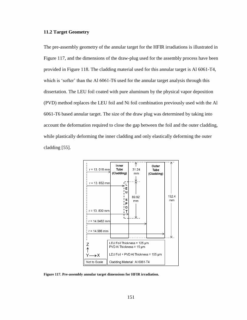
151

11.2 Target Geometry

The pre-assembly geometry of the annular target for the HFIR irradiations is illustrated in

Figure 117, and the dimensions of the draw-plug used for the assembly process have been

provided in Figure 118. The cladding material used for this annular target is Al 6061-T4,

which is ‘softer’ than the Al 6061-T6 used for the annular target analysis through this

dissertation. The LEU foil coated with pure aluminum by the physical vapor deposition

(PVD) method replaces the LEU foil and Ni foil combination previously used with the Al

6061-T6 based annular target. The size of the draw plug was determined by taking into

account the deformation required to close the gap between the foil and the outer cladding,

while plastically deforming the inner cladding and only elastically deforming the outer

cladding [55].

Figure 117. Pre-assembly annular target dimensions for HFIR irradiation.

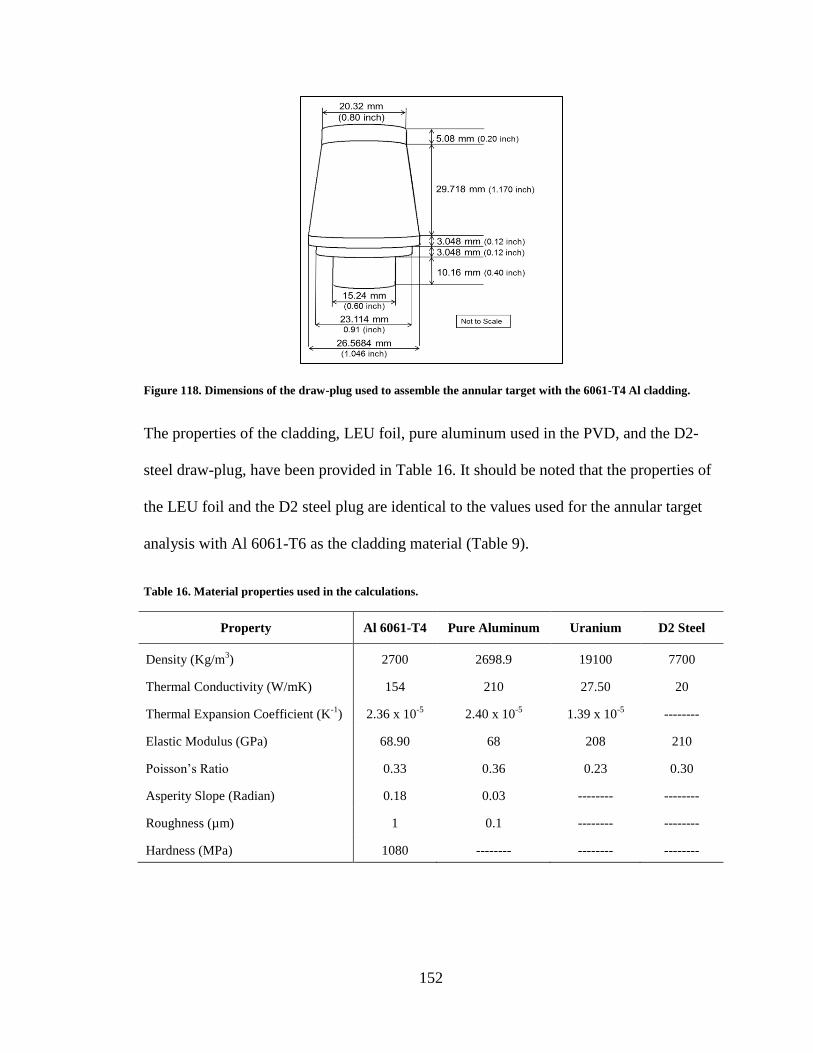
152

Figure 118. Dimensions of the draw-plug used to assemble the annular target with the 6061-T4 Al cladding.

The properties of the cladding, LEU foil, pure aluminum used in the PVD, and the D2-

steel draw-plug, have been provided in Table 16. It should be noted that the properties of

the LEU foil and the D2 steel plug are identical to the values used for the annular target

analysis with Al 6061-T6 as the cladding material (Table 9).

Table 16. Material properties used in the calculations.

Property Al 6061-T4 Pure Aluminum Uranium D2 Steel

Density (Kg/m3) 2700 2698.9 19100 7700

Thermal Conductivity (W/mK) 154 210 27.50 20


) 2.36 x 10-5

2.40 x 10-5

1.39 x 10-5

--------


Poisson’s Ratio 0.33 0.36 0.23 0.30

Asperity Slope (Radian) 0.18 0.03 -------- --------

Roughness (µm) 1 0.1 -------- --------

Hardness (MPa) 1080 -------- -------- --------

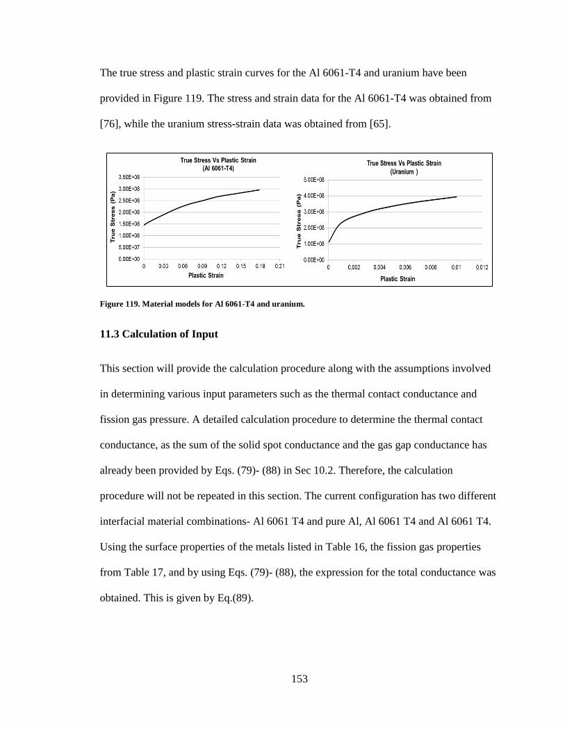
153

The true stress and plastic strain curves for the Al 6061-T4 and uranium have been

provided in Figure 119. The stress and strain data for the Al 6061-T4 was obtained from

[76], while the uranium stress-strain data was obtained from [65].

Figure 119. Material models for Al 6061-T4 and uranium.

11.3 Calculation of Input

This section will provide the calculation procedure along with the assumptions involved

in determining various input parameters such as the thermal contact conductance and

fission gas pressure. A detailed calculation procedure to determine the thermal contact

conductance, as the sum of the solid spot conductance and the gas gap conductance has

already been provided by Eqs. (79)- (88) in Sec 10.2. Therefore, the calculation

procedure will not be repeated in this section. The current configuration has two different

interfacial material combinations- Al 6061 T4 and pure Al, Al 6061 T4 and Al 6061 T4.

Using the surface properties of the metals listed in Table 16, the fission gas properties

from Table 17, and by using Eqs. (79)- (88), the expression for the total conductance was

obtained. This is given by Eq.(89).

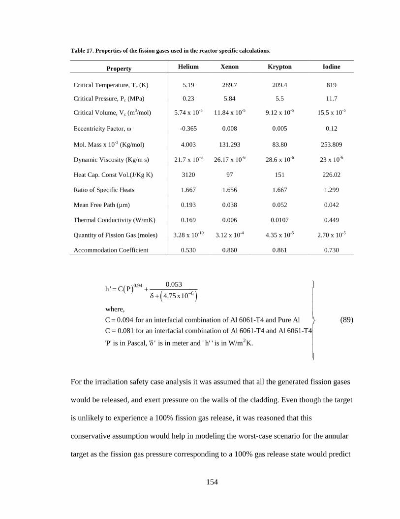
154

Table 17. Properties of the fission gases used in the reactor specific calculations.

Property Helium Xenon Krypton Iodine

Critical Temperature, Tc (K) 5.19 289.7 209.4 819

Critical Pressure, Pc (MPa) 0.23 5.84 5.5 11.7

Critical Volume, Vc (m3/mol) 5.74 x 10

-5 11.84 x 10

-5 9.12 x 10

-5 15.5 x 10

-5

Eccentricity Factor, ω -0.365 0.008 0.005 0.12

Mol. Mass x 10-3

(Kg/mol)

4.003

131.293

83.80

253.809

Dynamic Viscosity (Kg/m s)

21.7 x 10-6

26.17 x 10-6

28.6 x 10-6

23 x 10-6

Heat Cap. Const Vol.(J/Kg K)

3120

97

151

226.02

Ratio of Specific Heats

1.667

1.656

1.667

1.299

Mean Free Path (µm)

0.193

0.038

0.052

0.042

Thermal Conductivity (W/mK)

0.169

0.006

0.0107

0.449

Quantity of Fission Gas (moles)

3.28 x 10-10

3.12 x 10-4

4.35 x 10-5

2.70 x 10-5

Accommodation Coefficient

0.530

0.860

0.861

0.730

0.94

6

0.053h ' C P

4.75x10

where,

C 0.094 for an interfacial combination of Al 6061-T4 and Pure Al

C = 0.081 for an interfacial combination of Al 6061-T4 and Al 6061-T4

'P' is in Pascal, ' ' is in meter

2

and ' h' ' is in W/m K.

(89)

For the irradiation safety case analysis it was assumed that all the generated fission gases

would be released, and exert pressure on the walls of the cladding. Even though the target

is unlikely to experience a 100% fission gas release, it was reasoned that this

conservative assumption would help in modeling the worst-case scenario for the annular

target as the fission gas pressure corresponding to a 100% gas release state would predict

155

a higher irradiation thermal stress margin as compared to when the percentage of gas

release, and hence the fission gas pressure is lower. The procedure to calculate the fission

gas pressure has already been outlined in Sec 10.1 and is given by Eqs. (66)-(75). Using

these equations along with the fission gas data given in Table 17, the fission gas pressure

corresponding to a 100 % gas release situation was found to be 7.5 MPa. Uranium

swelling effects were not included in the model as there was a lot of uncertainty, at that

point, over selecting the best approach to model the swelling effects. Therefore, this

aspect was left to the independent reviewer of the calculation to address.

The coolant flow velocity for this irradiation experiment was to be 6.09 m/s. Taking the

density of water as 984.55 Kg/m3, the dynamic viscosity as 487 x 10

-6 Kg/m-s, thermal

conductivity as 0.650 W/mK, Prandtl number as 3.1348, along with the dimensions from

Figure 117, and the Nusselt number correlations for fully developed turbulent flow given

by Eqs. (6)-(7), the surface heat transfer coefficient for the inner tube was found to be

30118.3 W/m2K, and for flow over the outer tube was 32220.5 W/m

2K.

11.4 Finite Element Model Development

The commercial finite element code Abaqus FEA [56] was used to first model the draw-

plug assembly process of the annular target, and then use the residual stress results in a

separate irradiation model. It should be noted that the successive three-step analysis

procedure, outlined in Sec.9 and Sec. 10, was developed towards the later part of 2013.

The safety analysis was completed using the procedure outlined in this section. The draw-

plug assembly process was the preferred method to assemble the annular targets for the

HFIR irradiation. In this process, pure aluminum is deposited on the edges of the LEU

156

foil using a process known as physical vapor deposition (PVD). Following this, the foil

with Al coating is wrapped around the inner Al 6061-T4 tube and slid into the outer Al

6061-T4 tube. This combination is placed inside a draw-die and a tapered plug is driven

through the inner tube. This expands the inner tube, which in-turn pushes the foil towards

the outer tube and enforces interfacial contact. The draw plug assembly process is

designed to plastically deform the inner tube and elastically deform the outer tube. After

assembly, the ends of the target are welded to provide a completely sealed environment.

Due to the difficulty associated with physically measuring certain dimensions of the

annular target assembly, it was decided to simulate the assembly process by means of an

axisymmetric stress analysis, using the commercial finite element code Abaqus FEA. The

dimensions of the annular target obtained from the assembly were used to build an

irradiation model, by including the assembly residual stresses as an initial input. The

purpose of the irradiation model is to simulate the in-vessel irradiation by accounting for

the volumetric heat generation in the LEU foil, gamma heating in the cladding, fission

gas release.

The draw-plug assembly model was setup using the dimensions of the annular target

from Figure 117 and the material properties from Table 16. The end of the target, away

from the plug, was not allowed to translate in the longitudinal direction, as this is the case

during the draw-plug assembly procedure. The assembly model does not have any

external loading conditions imposed on it. As the plug moves through the inner tube, a

velocity boundary condition was applied to the based of the plug. The radial and

rotational velocity components were set to zero, while the longitudinal velocity

component was enabled. As the applied drawing force to the plug was unknown to the

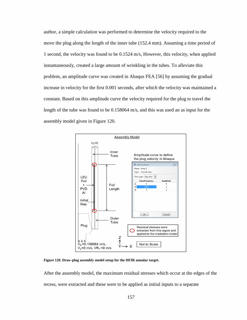
157

author, a simple calculation was performed to determine the velocity required to the

move the plug along the length of the inner tube (152.4 mm). Assuming a time period of

1 second, the velocity was found to be 0.1524 m/s, However, this velocity, when applied

instantaneously, created a large amount of wrinkling in the tubes. To alleviate this

problem, an amplitude curve was created in Abaqus FEA [56] by assuming the gradual

increase in velocity for the first 0.001 seconds, after which the velocity was maintained a

constant. Based on this amplitude curve the velocity required for the plug to travel the

length of the tube was found to be 0.158064 m/s, and this was used an as input for the

assembly model given in Figure 120.

Figure 120. Draw-plug assembly model setup for the HFIR annular target.

After the assembly model, the maximum residual stresses which occur at the edges of the

recess, were extracted and these were to be applied as initial inputs to a separate

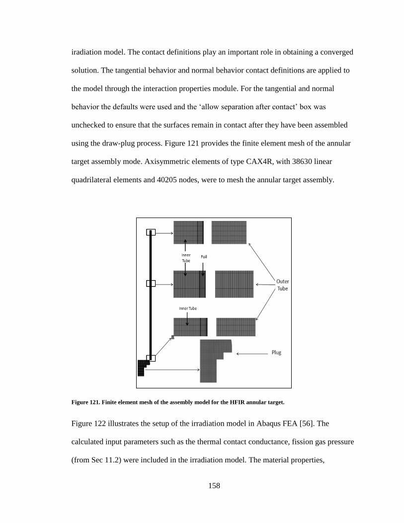
158

iradiation model. The contact definitions play an important role in obtaining a converged

solution. The tangential behavior and normal behavior contact definitions are applied to

the model through the interaction properties module. For the tangential and normal

behavior the defaults were used and the ‘allow separation after contact’ box was

unchecked to ensure that the surfaces remain in contact after they have been assembled

using the draw-plug process. Figure 121 provides the finite element mesh of the annular

target assembly mode. Axisymmetric elements of type CAX4R, with 38630 linear

quadrilateral elements and 40205 nodes, were to mesh the annular target assembly.

Figure 121. Finite element mesh of the assembly model for the HFIR annular target.

Figure 122 illustrates the setup of the irradiation model in Abaqus FEA [56]. The

calculated input parameters such as the thermal contact conductance, fission gas pressure

(from Sec 11.2) were included in the irradiation model. The material properties,

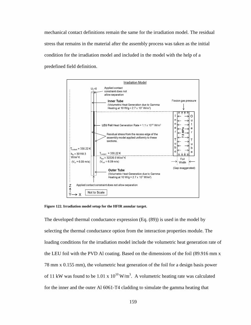
159

mechanical contact definitions remain the same for the irradiation model. The residual

stress that remains in the material after the assembly process was taken as the initial

condition for the irradiation model and included in the model with the help of a

predefined field definition.

Figure 122. Irradiation model setup for the HFIR annular target.

The developed thermal conductance expression (Eq. (89)) is used in the model by

selecting the thermal conductance option from the interaction properties module. The

loading conditions for the irradiation model include the volumetric heat generation rate of

the LEU foil with the PVD Al coating. Based on the dimensions of the foil (89.916 mm x

78 mm x 0.155 mm), the volumetric heat generation of the foil for a design basis power

of 11 kW was found to be 1.01 x 1010

W/m3. A volumetric heating rate was calculated

for the inner and the outer Al 6061-T4 cladding to simulate the gamma heating that

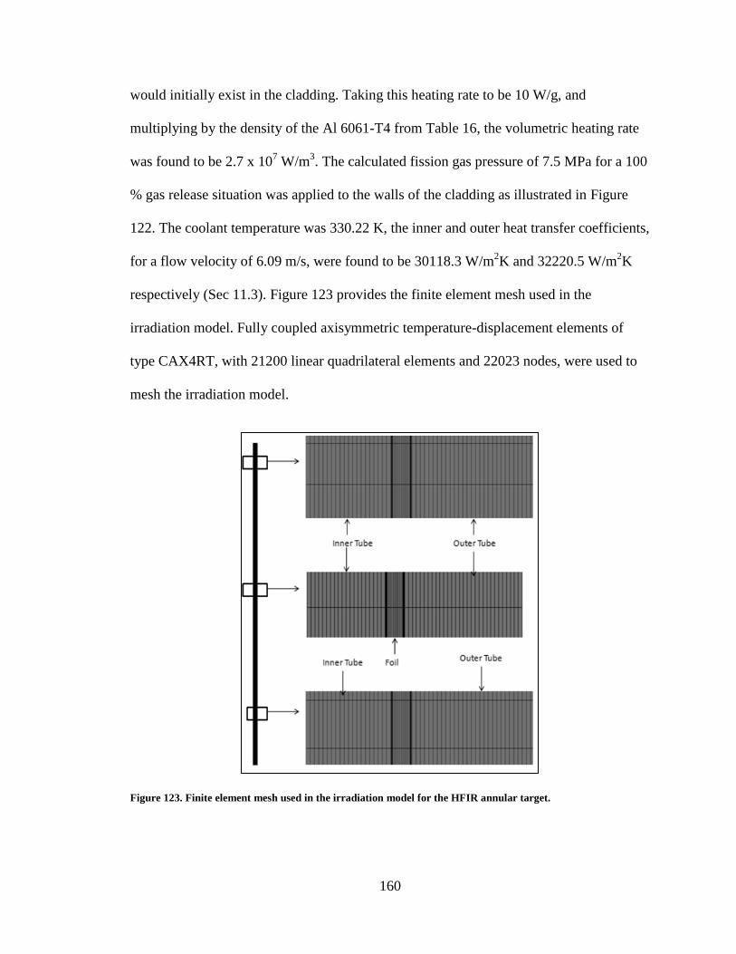
160

would initially exist in the cladding. Taking this heating rate to be 10 W/g, and

multiplying by the density of the Al 6061-T4 from Table 16, the volumetric heating rate

was found to be 2.7 x 107 W/m

3. The calculated fission gas pressure of 7.5 MPa for a 100

% gas release situation was applied to the walls of the cladding as illustrated in Figure

122. The coolant temperature was 330.22 K, the inner and outer heat transfer coefficients,

for a flow velocity of 6.09 m/s, were found to be 30118.3 W/m2K and 32220.5 W/m

2K

respectively (Sec 11.3). Figure 123 provides the finite element mesh used in the

irradiation model. Fully coupled axisymmetric temperature-displacement elements of

type CAX4RT, with 21200 linear quadrilateral elements and 22023 nodes, were used to

mesh the irradiation model.

Figure 123. Finite element mesh used in the irradiation model for the HFIR annular target.

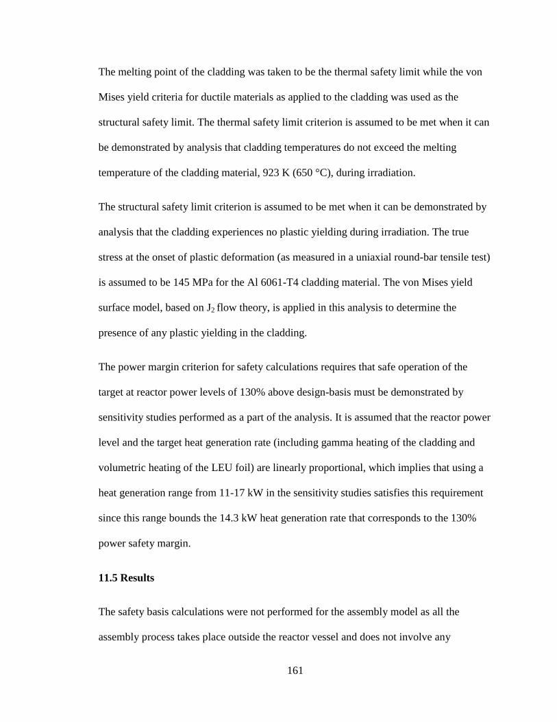
161

The melting point of the cladding was taken to be the thermal safety limit while the von

Mises yield criteria for ductile materials as applied to the cladding was used as the

structural safety limit. The thermal safety limit criterion is assumed to be met when it can

be demonstrated by analysis that cladding temperatures do not exceed the melting

temperature of the cladding material, 923 K (650 °C), during irradiation.

The structural safety limit criterion is assumed to be met when it can be demonstrated by

analysis that the cladding experiences no plastic yielding during irradiation. The true

stress at the onset of plastic deformation (as measured in a uniaxial round-bar tensile test)

is assumed to be 145 MPa for the Al 6061-T4 cladding material. The von Mises yield

surface model, based on J2 flow theory, is applied in this analysis to determine the

presence of any plastic yielding in the cladding.

The power margin criterion for safety calculations requires that safe operation of the

target at reactor power levels of 130% above design-basis must be demonstrated by

sensitivity studies performed as a part of the analysis. It is assumed that the reactor power

level and the target heat generation rate (including gamma heating of the cladding and

volumetric heating of the LEU foil) are linearly proportional, which implies that using a

heat generation range from 11-17 kW in the sensitivity studies satisfies this requirement

since this range bounds the 14.3 kW heat generation rate that corresponds to the 130%

power safety margin.

11.5 Results

The safety basis calculations were not performed for the assembly model as all the

assembly process takes place outside the reactor vessel and does not involve any

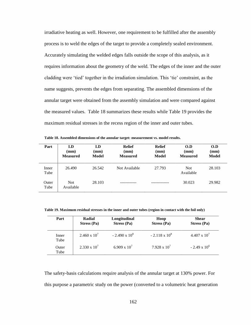
162

irradiative heating as well. However, one requirement to be fulfilled after the assembly

process is to weld the edges of the target to provide a completely sealed environment.

Accurately simulating the welded edges falls outside the scope of this analysis, as it

requires information about the geometry of the weld. The edges of the inner and the outer

cladding were ‘tied’ together in the irradiation simulation. This ‘tie’ constraint, as the

name suggests, prevents the edges from separating. The assembled dimensions of the

annular target were obtained from the assembly simulation and were compared against

the measured values. Table 18 summarizes these results while Table 19 provides the

maximum residual stresses in the recess region of the inner and outer tubes.

Table 18. Assembled dimensions of the annular target: measurement vs. model results.

Part I.D

(mm)

Measured

I.D

(mm)

Model

Relief

(mm)

Measured

Relief

(mm)

Model

O.D

(mm)

Measured

O.D

(mm)

Model

Inner

Tube

26.490 26.542 Not Available 27.793 Not

Available

28.103

Outer

Tube

Not

Available

28.103 ------------ ------------- 30.023 29.982

Table 19. Maximum residual stresses in the inner and outer tubes (region in contact with the foil only)

Part Radial

Stress (Pa)

Longitudinal

Stress (Pa)

Hoop

Stress (Pa)

Shear

Stress (Pa)

Inner

Tube

2.460 x 107 - 2.490 x 10

8 - 2.118 x 10

8 4.407 x 10

7

Outer

Tube

2.330 x 107 6.909 x 10

7 7.928 x 10

7 - 2.49 x 10

6

The safety-basis calculations require analysis of the annular target at 130% power. For

this purpose a parametric study on the power (converted to a volumetric heat generation

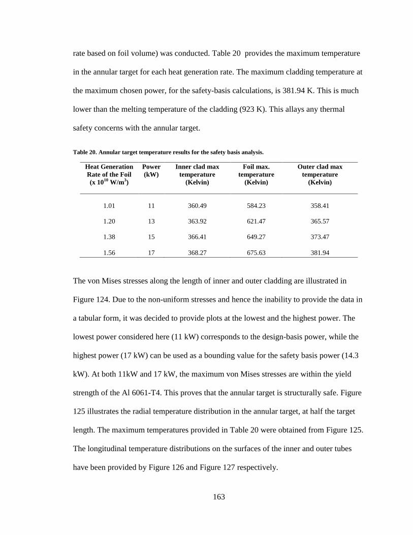
163

rate based on foil volume) was conducted. Table 20 provides the maximum temperature

in the annular target for each heat generation rate. The maximum cladding temperature at

the maximum chosen power, for the safety-basis calculations, is 381.94 K. This is much

lower than the melting temperature of the cladding (923 K). This allays any thermal

safety concerns with the annular target.

Table 20. Annular target temperature results for the safety basis analysis.

Heat Generation

Rate of the Foil

(x 1010

W/m3)

Power

(kW)

Inner clad max

temperature

(Kelvin)

Foil max.

temperature

(Kelvin)

Outer clad max

temperature

(Kelvin)

1.01

11

360.49

584.23

358.41

1.20

13

363.92

621.47

365.57

1.38

15

366.41

649.27

373.47

1.56

17

368.27

675.63

381.94

The von Mises stresses along the length of inner and outer cladding are illustrated in

Figure 124. Due to the non-uniform stresses and hence the inability to provide the data in

a tabular form, it was decided to provide plots at the lowest and the highest power. The

lowest power considered here (11 kW) corresponds to the design-basis power, while the

highest power (17 kW) can be used as a bounding value for the safety basis power (14.3

kW). At both 11kW and 17 kW, the maximum von Mises stresses are within the yield

strength of the Al 6061-T4. This proves that the annular target is structurally safe. Figure

125 illustrates the radial temperature distribution in the annular target, at half the target

length. The maximum temperatures provided in Table 20 were obtained from Figure 125.

The longitudinal temperature distributions on the surfaces of the inner and outer tubes

have been provided by Figure 126 and Figure 127 respectively.

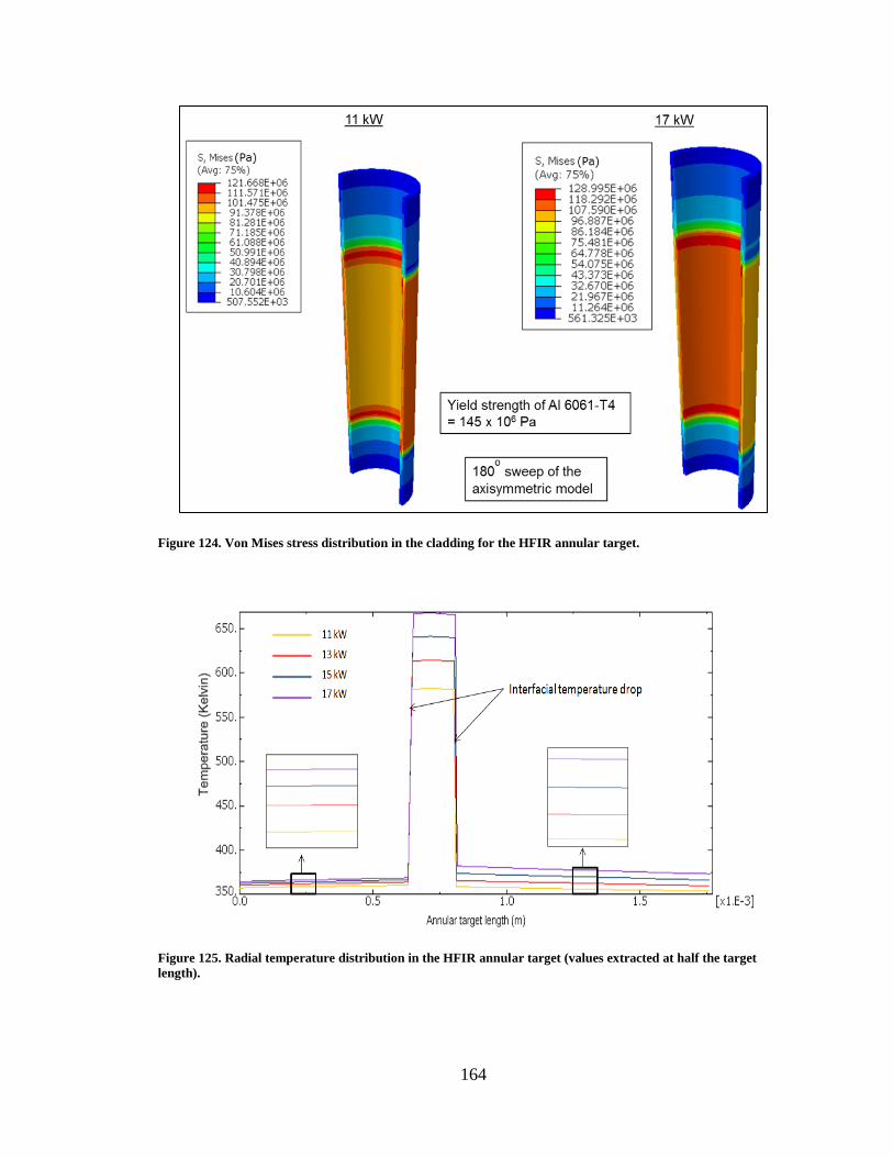
164

Figure 124. Von Mises stress distribution in the cladding for the HFIR annular target.

Figure 125. Radial temperature distribution in the HFIR annular target (values extracted at half the target

length).

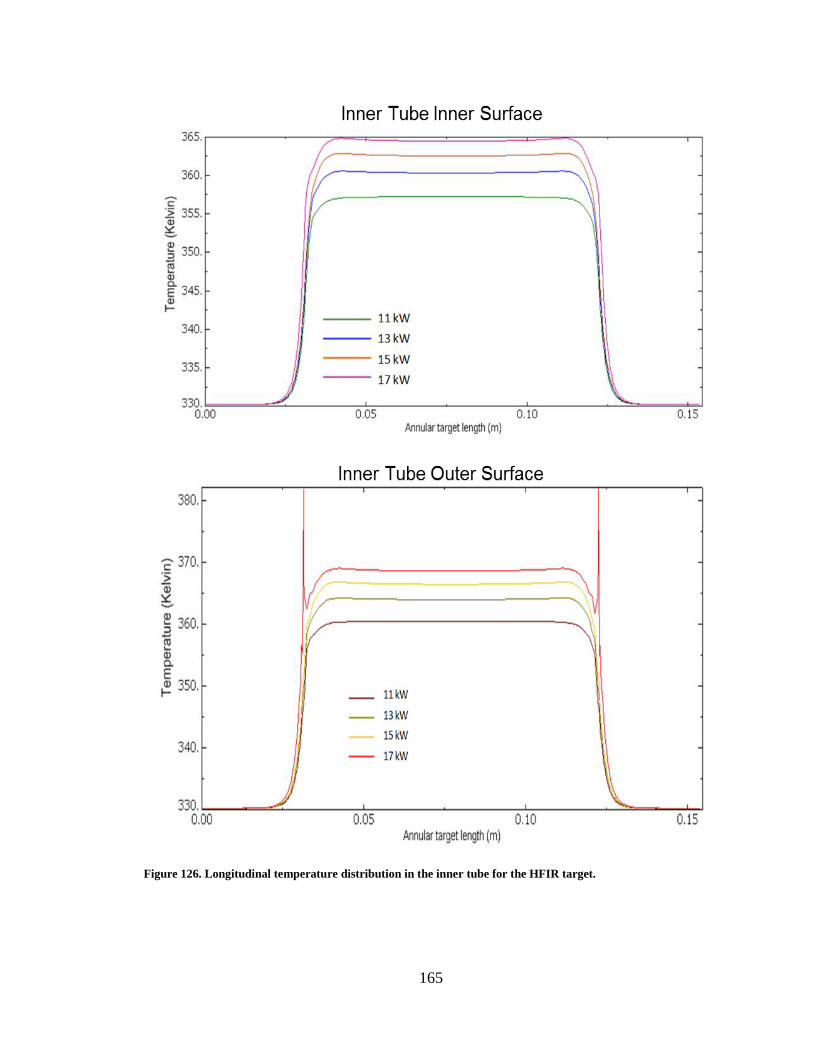
165

Figure 126. Longitudinal temperature distribution in the inner tube for the HFIR target.

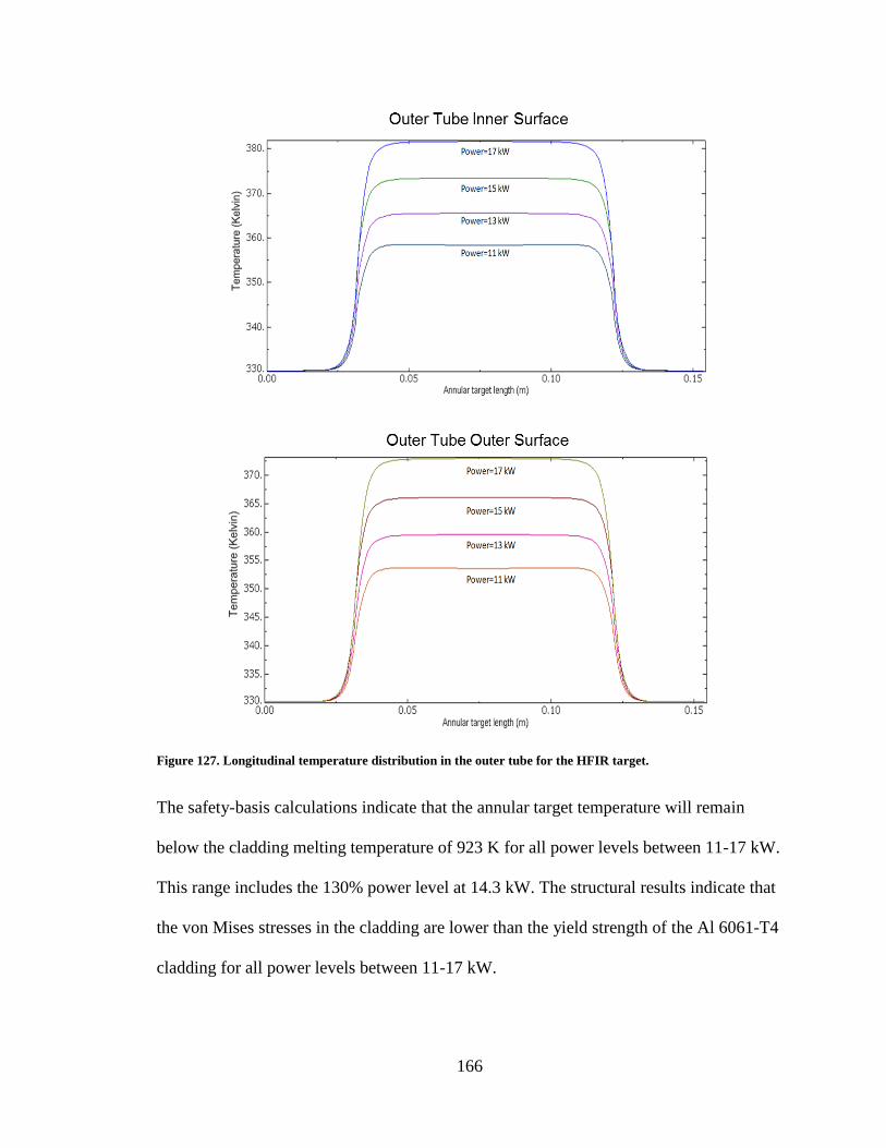
166

Figure 127. Longitudinal temperature distribution in the outer tube for the HFIR target.

The safety-basis calculations indicate that the annular target temperature will remain

below the cladding melting temperature of 923 K for all power levels between 11-17 kW.

This range includes the 130% power level at 14.3 kW. The structural results indicate that

the von Mises stresses in the cladding are lower than the yield strength of the Al 6061-T4

cladding for all power levels between 11-17 kW.

167

11.6 Comments from the Technical Adequacy and Independent Review Committee

One of the requirements to be fulfilled before the calculation is formally accepted is that

it should pass the technical adequacy review and the independent review. The developed

calculation was approved by the committee and their respective conclusions have been

provided below in quotations.

“A check and technical adequacy review (TAR) has been carried out for the safety-basis

SBP-1000 analysis documented in “Mechanical and Thermal-Stress Analysis of an

Annular Target with a Low-Enriched Uranium Foil for HFIR Irradiation,”

C-HFIR-2013-023, prepared by S.G. Govindarajan. This TAR, guided by the Technical

Adequacy Review Checklist (SBPF-1000.1) shown on p. 1 of this document, was

performed pursuant to the procedures given in “Preparation, Review, and Handling of

Calculations” SBP-1000, rev. 2, and “Configuration Controls of Software for HFIR

Safety Basis Calculations,” SBP-1300, rev. 1, where applicable. All inputs were checked

to ensure that the values reported in C-HFIR-2013-023 correctly reflected the values

applied in the Abaqus input files. All significant assumptions were identified and

adequately justified in the document. Selected Abaqus baseline cases were re-run by the

author of this TAR to check that the results reported in C-HFIR-2013-023 could be easily

identified in the Abaqus output by any future re-analysis of the target assembly. A

“separate-effects” study was carried out for this TAR for the purpose of checking the

sensitivity of the analysis results to small modifications to the input data by identifying

and applying different (but still valid) modeling decisions and assumptions. The results of

the study indicated that small changes to the inputs produced small changes in the

output, and the changes in the results followed trends expected from the physics being

simulated by the model.”

- Technical Adequacy Reviewer

“This independent review of C-HFIR-2013-023/R0 has determined that the calculation is

technically adequate (the models employed are generally text-book and have been used

extensively in the current fuel performance codes that are available today). Also, a

critique (Sections 3.2.2 through 3.2.5, above) of the assumptions employed in the

calculation irradiation modeling indicate that these assumptions are overly conservative;

that is, the calculated gas gap conductances are probably conservatively low which

results in higher calculated foil temperatures.”

- Independent Reviewer

168

Chapter 12: Boral Control Blade Safety Analysis

This chapter will focus on the 2nd

part of this dissertation – safety analysis of a nuclear

reactor component. The analysis presented in this section was performed by the author of

this dissertation for MURR to help them with their relicensing efforts. The work [77] was

presented at the 5th

international symposium for material testing reactors (ISMTR) held in

Columbia, Missouri.

12.1 Control Blade Geometry and Model Development

Since a detailed introduction of the BORAL [78] control blades used at MURR has

already been provided in Sec 1.4, this section will first introduce the geometry of the

control blade followed by the model development.

The neutron absorber in the BORAL [78] control blades at MURR is boron. The control

blades operate in a gap between the outside of the reactor pressure vessel and the inside

of the beryllium reflector as shown in Figure 7. The BORAL core geometry is 0.863 m

long, 0.254 x 10-2

m thick and 0.205 m wide. The radius of curvature of the centerline of

the blade is 0.166 m. The aluminum cladding thickness of 9.5 x 10-4

m on the front and

back faces of the BORAL with 0.003 m on both edges. The mounting region of the blade

extends to 0.139 m beyond the BORAL cavity. Thus the overall profile of the control

blade including the mounting region is 0.211 m wide x 0.004 m thick x 0.101 m long.

The geometry of the control blade has been provided in Figure 128. The outer diameter of

the pressure vessel is between 0.318m and 0.319m. The inner diameter of the beryllium

reflector is between 0.347m and 0.348 m. The gap width is maintained by vertical spacers

which are set into the beryllium reflector and cross the gap to the outer diameter of the

169

reactor pressure vessel. The minimum width of the gap in which the rods operate is 1.4 x

10-2

m. The thickness of the control blade is 0.635 x 10-2

m, leaving a gap of

approximately 0.381 x 10-2

m on either side of the blade [79]. The displacement of the

blade would be as a result of differential expansion between the inner and outer

longitudinal fibers with a radial temperature gradient through the blade.

Figure 128. Dimensions of the BORAL control blade at the Missouri University Research Reactor (MURR).

The energy deposition in a highly discretized model of a MURR control blade, that can

be in any four possible positions “A”, “B”, “C” or “D” of the MURR core configuration,

was studied using the Monte Carlo N-Particle (MCNP) model [80] by Nickie J. Peters

[81] from MURR. A control blade of nominal length 0.863 m, placed in any one of these

positions, travels within a narrow annular water channel between the outer surface of the

outer reactor pressure vessel and the inner wall of the beryllium reflector, which is 1.42 x

10-2

m wide. Figure 129 provides the cross sectional view [82] of the MCNP MURR core

model showing the four control blade positions. For the MCNP [80] computations, the

control blade was divided into 154 independent zones (cells), which include: (i) 4

azimuthal sections (over the entire length), (ii) 9 radial sections over each of the 4

incremental unit length sections for each azimuthal section, and (iii) 2 radial sections over

170

each of the next five incremental sections for each azimuthal section. The discretization

scheme was chosen to properly account for correct spatial distribution of the energy

release from the 10

B(n, α)6Li reaction, the major component of the energy deposited in

the blade. The increase discretization in the (four) lowest portions reflect the most active

regions of the control blade.

Figure 129. A cross- sectional view of the MCNP MURR core model showing the four positions of the control

blades in a narrow water channel between the outer surface of the outer reactor pressure vessel and the inner

wall of the beryllium reflector.

The F6 neutron tally in MCNP [80] was used to recover the energy-release from the 10

B

fission within the blade. Since the second most significant source of energy deposition in

the control blade comes from gamma rays, that mostly originate from uranium fission in

the fuel and (n, γ) capture interactions throughout the core, the F6 photon tally in MCNP

[80] in addition to the method described [81] was used to predict this contribution. Since

the energy deposited from the 10

B(n, α)6Li reaction and the gamma interactions have

different origins, their energy deposition profiles throughout the blade are expected to be

different. This is important because deflection in the blade is directly related to the

magnitudes of thermal stresses across different regions in the blade. The energy

deposition profiles (i.e., alpha + gamma) determine how the heating rate varies

throughout the blade as it is being irradiated. The bottom of the blade is predicted to be

B

A

D

C

Control

Blade

Water

Channel

171

the region of highest energy deposition. This is expected since the bottom edge of the

control blade is always constrained to be within the length of the fuel even at maximum

travel.

12.2 Heating Profile Development

The BORAL meat was split into 4 quadrants. The heat generation rate as a function of the

thickness and longitudinal position due to radiative heating was calculated. A curve fit

was created using the discrete points obtained from the MCNP [80] simulations. The data

at the longitudinal locations 0.259 m, 0.432 m, 0.604 m and 0.777 m from the fuel-side

aluminum cladding and beryllium side aluminum cladding were used for the heat

generation values within the BORAL thickness Fuel-side data points were considered

constant through the first four BORAL thickness locations. Beryllium side data points

were considered constant through the last four BORAL thickness locations. The data

point at the center of the BORAL was averaged from the fuel side and beryllium side

points. For a given azimuthal position, the volumetric heat generation data was plotted

against thickness and longitudinal position using 3-D plotting software to visualize the

general functional trends. Additionally, for a given thickness, the data was plotted against

azimuthal and longitudinal position to further aid in visualization. These plots suggested

that the volumetric heat generation follows an even polynomial profile in the radial

direction, t, and a decaying exponential in the longitudinal direction, z. Hence, a function

of the form given by Eq. (90) was assumed, where the functions A(t) and B(t) allow for a

different decaying functions to be determined at a given radial position.

B t zq ''' f t, z A t e (90)

172

A function of this form was determined for each of the four partitions the blade was

divided into, the left edge, left middle, right middle and right edge quadrants. The

equation governing the left edge section was held constant along the azimuthal direction

between -36.3˚ and -18.15˚. The equation governing the left middle section was held

constant along the azimuthal direction for -18.15˚ to 0˚. Likewise, the right middle

section applied to the 0˚ to 18.15˚ portion of the blade and the right edge equation applied

to the 18.15˚ to 36.3˚ partition. To derive the functions A(t) and B(t), the natural

logarithm of Eq. (90) to obtain Eq. (91).

ln q ''' ln A t B t z C t (91)

Using the above equation it is simple to fit a straight line relating the ln (q"') to z at each

thickness location. An example of this process can be seen in the Figure 130where ln q′′′

is plotted against z at the BORAL fuel-side surface (t = 9.5 x 10-4

m) at the left edge

location for alpha heat generation. The slope and intercept are provided on the plot, with

the slope being the value of B and intercept the value of C. Equations of the form of Eq.

(91) were determined for each of the provided thickness and azimuthal locations. These

equations were then used as the exponent of the exponential function to return it to the

form of Eq.(90). Similar results were obtained for the gamma heating profile. The A and

B coefficient variation with thickness was then determined. Due to the discontinuities

occurring at the interfaces of the aluminum cladding and BORAL core, the overall

function for volumetric heat generation was defined in a piecewise fashion where the A

and B coefficients remained constant with thickness through the cladding on the fuel-side

and beryllium-side, while the coefficients varied with thickness through the BORAL

core. The A coefficient variation followed a 4th

order polynomial for the alpha heating

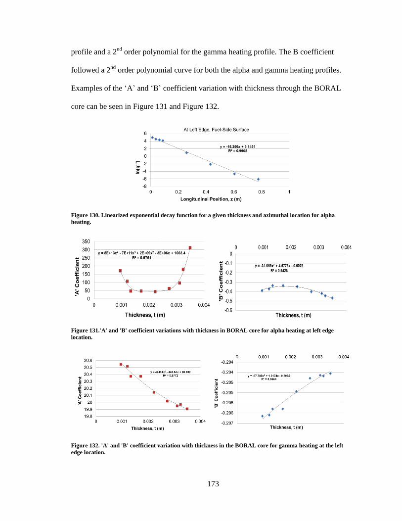
173

profile and a 2nd

order polynomial for the gamma heating profile. The B coefficient

followed a 2nd

order polynomial curve for both the alpha and gamma heating profiles.

Examples of the ‘A’ and ‘B’ coefficient variation with thickness through the BORAL

core can be seen in Figure 131 and Figure 132.

Figure 130. Linearized exponential decay function for a given thickness and azimuthal location for alpha

heating.

Figure 131.'A' and 'B' coefficient variations with thickness in BORAL core for alpha heating at left edge

location.

Figure 132. 'A' and 'B' coefficient variation with thickness in the BORAL core for gamma heating at the left

edge location.

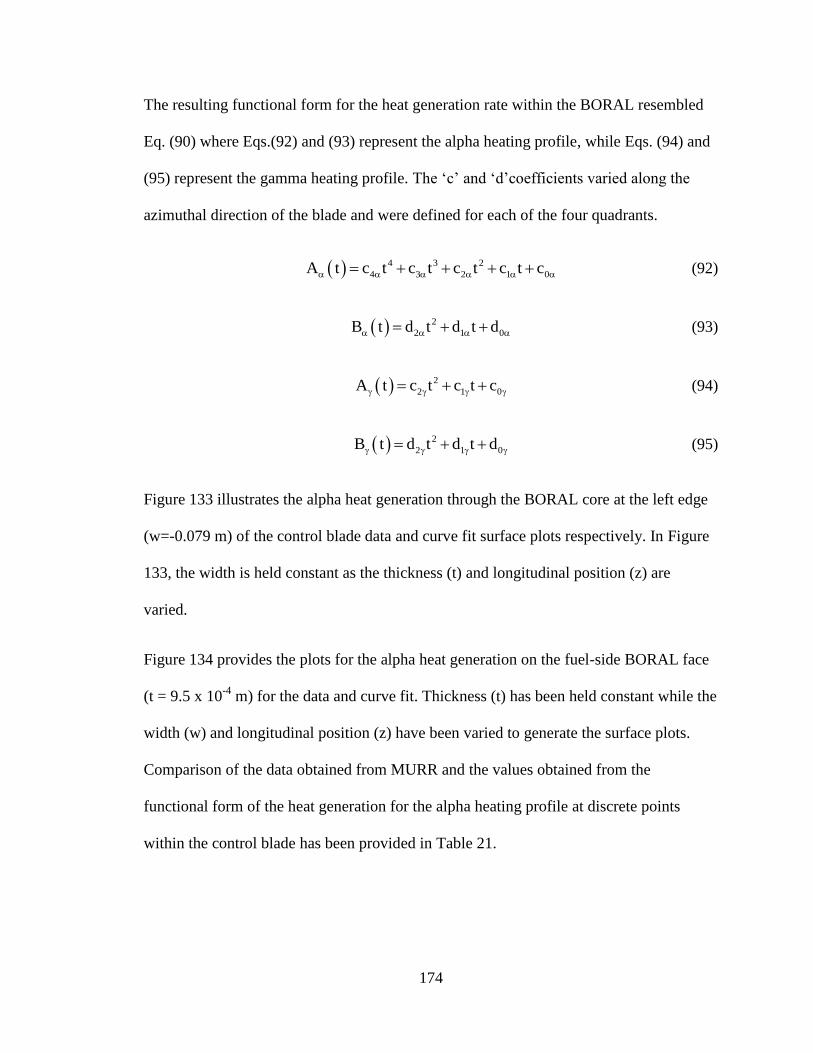
174

The resulting functional form for the heat generation rate within the BORAL resembled

Eq. (90) where Eqs.(92) and (93) represent the alpha heating profile, while Eqs. (94) and

(95) represent the gamma heating profile. The ‘c’ and ‘d’coefficients varied along the

azimuthal direction of the blade and were defined for each of the four quadrants.

4 3 2

4 3 2 1 0A t c t c t c t c t c (92)

2

2 1 0B t d t d t d (93)

2

2 1 0A t c t c t c (94)

2

2 1 0B t d t d t d (95)

Figure 133 illustrates the alpha heat generation through the BORAL core at the left edge

(w=-0.079 m) of the control blade data and curve fit surface plots respectively. In Figure

133, the width is held constant as the thickness (t) and longitudinal position (z) are

varied.

Figure 134 provides the plots for the alpha heat generation on the fuel-side BORAL face

(t = 9.5 x 10-4

m) for the data and curve fit. Thickness (t) has been held constant while the

width (w) and longitudinal position (z) have been varied to generate the surface plots.

Comparison of the data obtained from MURR and the values obtained from the

functional form of the heat generation for the alpha heating profile at discrete points

within the control blade has been provided in Table 21.

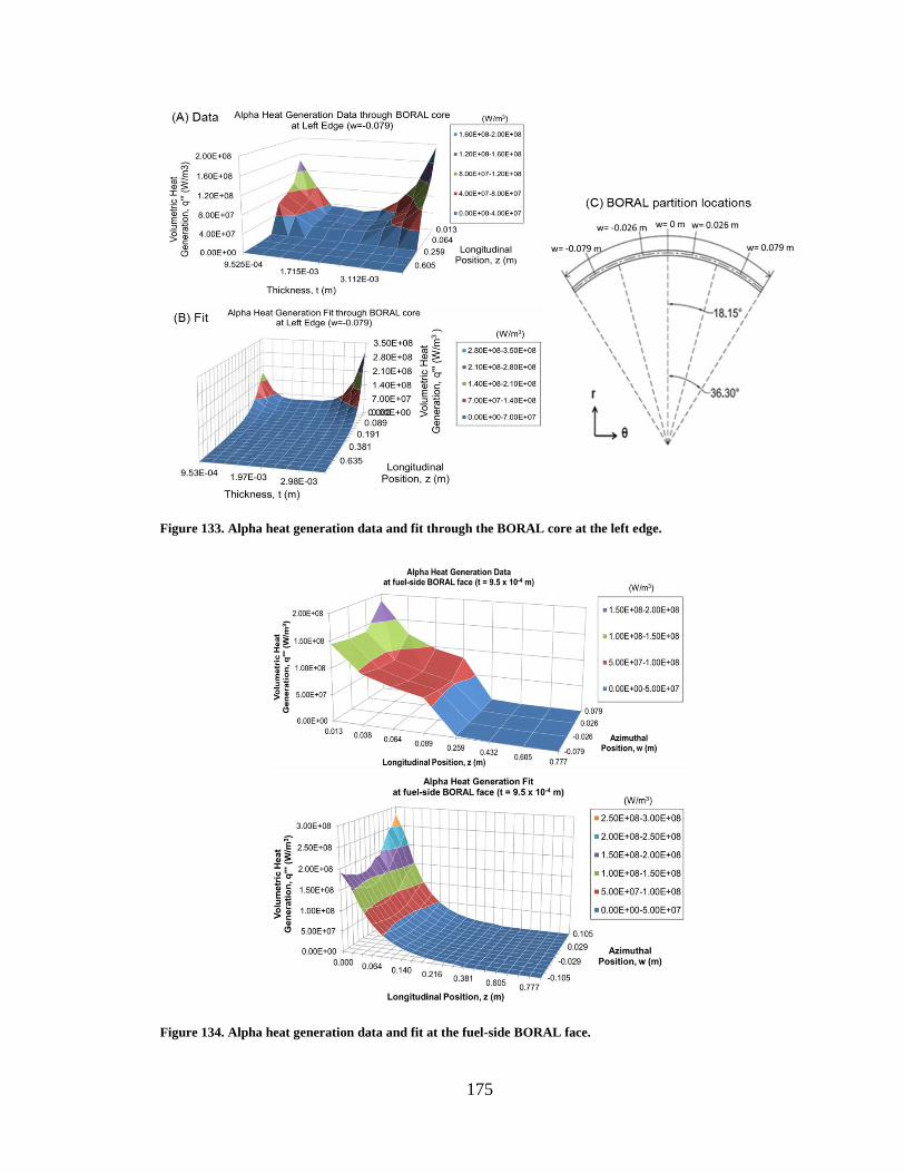
175

Figure 133. Alpha heat generation data and fit through the BORAL core at the left edge.

Figure 134. Alpha heat generation data and fit at the fuel-side BORAL face.

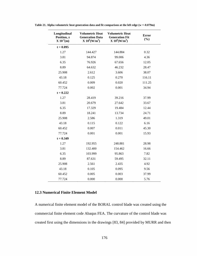
176

Table 21. Alpha volumetric heat generation data and fit comparison at the left edge (w =-0.079m)

Longitudinal

Position, z

X 10-2

(m)

Volumetric Heat

Generation Data

X 106(W/m

3)

Volumetric Heat

Generation Fit

X 106(W/m

3)

Error

(%)

t = 0.095

1.27 144.427 144.884 0.32

3.81 94.874 99.006 4.36

6.35 76.926 67.656 12.05

8.89 64.632 46.232 28.47

25.908 2.612 3.606 38.07

43.18 0.125 0.270 116.11

60.452 0.009 0.020 111.25

77.724 0.002 0.001 34.94

t = 0.222

1.27 28.419 39.216 37.99

3.81 20.679 27.642 33.67

6.35 17.329 19.484 12.44

8.89 18.241 13.734 24.71

25.908 2.586 1.319 49.01

43.18 0.115 0.122 6.16

60.452 0.007 0.011 45.30

77.724 0.001 0.001 15.93

t = 0.349

1.27 192.955 248.881 28.98

3.81 132.400 154.462 16.66

6.35 103.999 95.863 7.82

8.89 87.631 59.495 32.11

25.908 2.561 2.435 4.92

43.18 0.105 0.095 9.56

60.452 0.005 0.003 37.99

77.724 0.000 0.000 5.76


A numerical finite element model of the BORAL control blade was created using the

commercial finite element code Abaqus FEA. The curvature of the control blade was

created first using the dimensions in the drawings [83, 84] provided by MURR and then

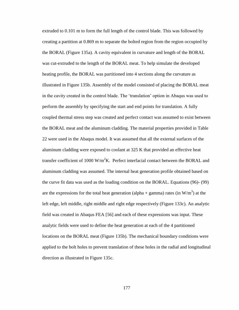
177

extruded to 0.101 m to form the full length of the control blade. This was followed by

creating a partition at 0.869 m to separate the bolted region from the region occupied by

the BORAL (Figure 135a). A cavity equivalent in curvature and length of the BORAL

was cut-extruded to the length of the BORAL meat. To help simulate the developed

heating profile, the BORAL was partitioned into 4 sections along the curvature as

illustrated in Figure 135b. Assembly of the model consisted of placing the BORAL meat

in the cavity created in the control blade. The ‘translation’ option in Abaqus was used to

perform the assembly by specifying the start and end points for translation. A fully

coupled thermal stress step was created and perfect contact was assumed to exist between

the BORAL meat and the aluminum cladding. The material properties provided in Table

22 were used in the Abaqus model. It was assumed that all the external surfaces of the

aluminum cladding were exposed to coolant at 325 K that provided an effective heat

transfer coefficient of 1000 W/m2K. Perfect interfacial contact between the BORAL and

aluminum cladding was assumed. The internal heat generation profile obtained based on

the curve fit data was used as the loading condition on the BORAL. Equations (96)- (99)

are the expressions for the total heat generation (alpha + gamma) rates (in W/m3) at the

left edge, left middle, right middle and right edge respectively (Figure 133c). An analytic

field was created in Abaqus FEA [56] and each of these expressions was input. These

analytic fields were used to define the heat generation at each of the 4 partitioned

locations on the BORAL meat (Figure 135b). The mechanical boundary conditions were

applied to the bolt holes to prevent translation of these holes in the radial and longitudinal

direction as illustrated in Figure 135c.

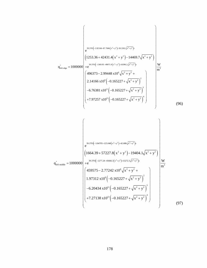
178

2 2 2 2

2 2 2 2

39.3701 2.82166 87.7846 x y 30.3262 x y z

2 2 2 2

39.3701 1369.95 49071.9 x y 16396.2 x y z'''

left edge

6 2 2

29 2 2

e

1253.36 42431.4 x y 14469.7 x y

q 1000000 e

496373 2.99448 x10 x y

2.14166 x10 0.165227 x y

6.76381 x

3

311 2 2

413 2 2

W

m

10 0.165227 x y

7.97257 x10 0.165227 x y

(96)

2 2 2 2

2 2 2 2

39.3701 3.84705 125.048 x y 42.688 x y z

2 2 2 2

39.3701 1277.24 45666.3 x y 15272.3 x y z'''

left middle

6 2 2

29 2 2

e

1664.39 57227.8 x y 19404.1 x y

q 1000000 e

459575 2.77242 x10 x y

1.97312 x10 0.165227 x y

6.20434

3

311 2 2

413 2 2

W

m

x10 0.165227 x y

7.27138 x10 0.165227 x y

(97)

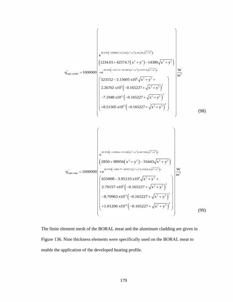
179

2 2 2 2

2 2 2 2

39.3701 4.09969 125.241 x y 44.241 x y z

2 2 2 2

39.3701 1317.27 47138.9 x y 15757.8 x y z'''

right middle

6 2 2

29 2 2

e

1234.01 42574.7 x y 14380 x y

q 1000000 e

523152 3.15605 x10 x y

2.26702 x10 0.165227 x y

7.1948 x1

3

311 2 2

413 2 2

W

m

0 0.165227 x y

8.51505 x10 0.165227 x y

(98)

2 2 2 2

2 2 2 2

39.3701 5.19054 173.182 x y 58.7592 x y z

2 2 2 2

39.3701 1281.77 45767.5 x y 15316.4 x y z'''

right edge

6 2 2

29 2 2

11

e

2850 98956 x y 33443 x y

q 1000000 e

655008 3.95133 x10 x y

2.79157 x10 0.165227 x y

8.70963 x10 0

3

32 2

414 2 2

W

m

.165227 x y

1.01206 x10 0.165227 x y

(99)

The finite element mesh of the BORAL meat and the aluminum cladding are given in

Figure 136. Nine thickness elements were specifically used on the BORAL meat to

enable the application of the developed heating profile.

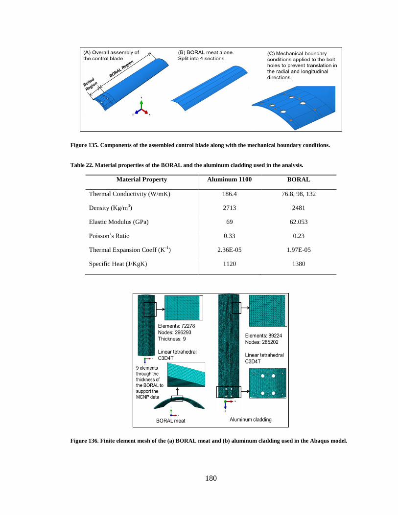
180

Figure 135. Components of the assembled control blade along with the mechanical boundary conditions.

Table 22. Material properties of the BORAL and the aluminum cladding used in the analysis.

Material Property Aluminum 1100 BORAL

Thermal Conductivity (W/mK) 186.4 76.8, 98, 132

Density (Kg/m3) 2713 2481

Elastic Modulus (GPa) 69 62.053

Poisson’s Ratio 0.33 0.23

Thermal Expansion Coeff (K-1

) 2.36E-05 1.97E-05

Specific Heat (J/KgK) 1120 1380

Figure 136. Finite element mesh of the (a) BORAL meat and (b) aluminum cladding used in the Abaqus model.

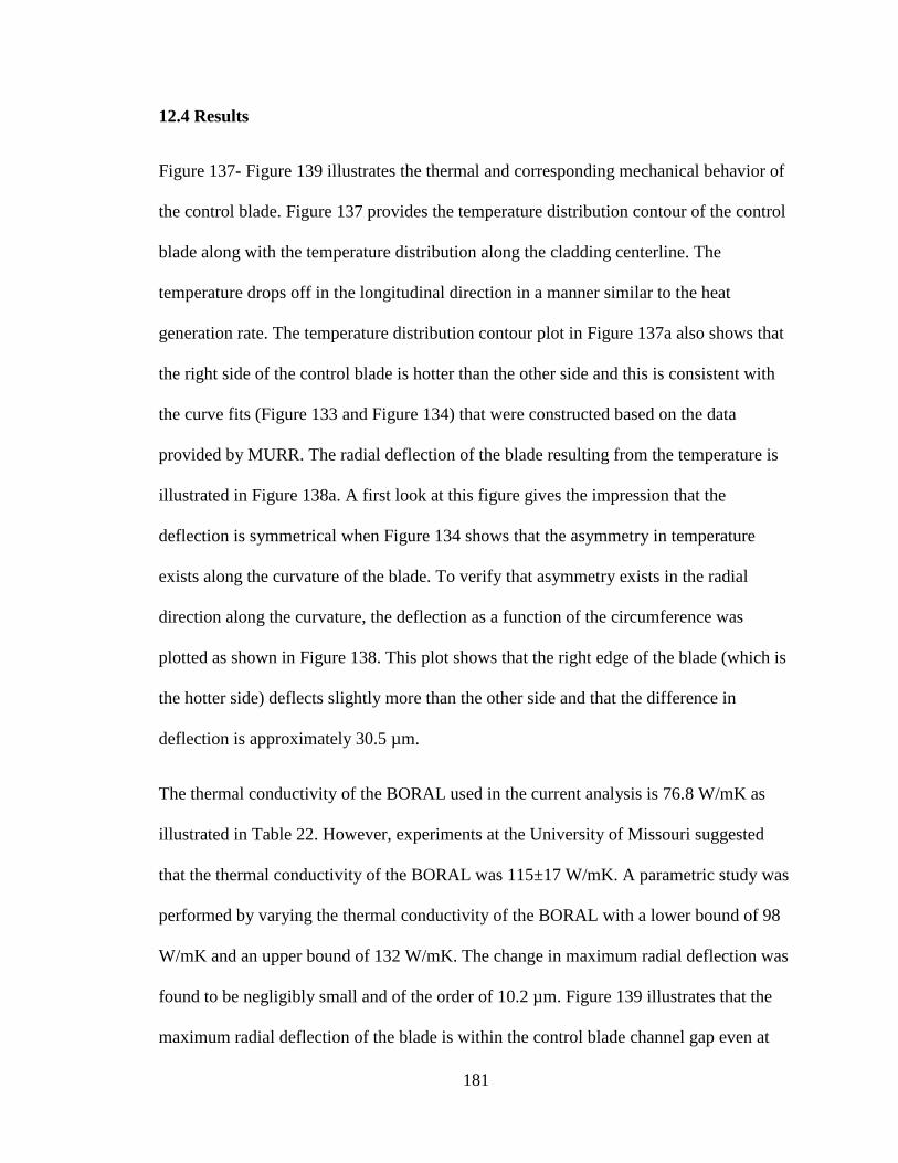
181

12.4 Results

Figure 137- Figure 139 illustrates the thermal and corresponding mechanical behavior of

the control blade. Figure 137 provides the temperature distribution contour of the control

blade along with the temperature distribution along the cladding centerline. The

temperature drops off in the longitudinal direction in a manner similar to the heat

generation rate. The temperature distribution contour plot in Figure 137a also shows that

the right side of the control blade is hotter than the other side and this is consistent with

the curve fits (Figure 133 and Figure 134) that were constructed based on the data

provided by MURR. The radial deflection of the blade resulting from the temperature is

illustrated in Figure 138a. A first look at this figure gives the impression that the

deflection is symmetrical when Figure 134 shows that the asymmetry in temperature

exists along the curvature of the blade. To verify that asymmetry exists in the radial

direction along the curvature, the deflection as a function of the circumference was

plotted as shown in Figure 138. This plot shows that the right edge of the blade (which is

the hotter side) deflects slightly more than the other side and that the difference in

deflection is approximately 30.5 µm.

The thermal conductivity of the BORAL used in the current analysis is 76.8 W/mK as

illustrated in Table 22. However, experiments at the University of Missouri suggested

that the thermal conductivity of the BORAL was 115±17 W/mK. A parametric study was

performed by varying the thermal conductivity of the BORAL with a lower bound of 98

W/mK and an upper bound of 132 W/mK. The change in maximum radial deflection was

found to be negligibly small and of the order of 10.2 µm. Figure 139 illustrates that the

maximum radial deflection of the blade is within the control blade channel gap even at

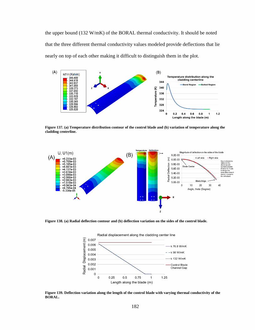
182

the upper bound (132 W/mK) of the BORAL thermal conductivity. It should be noted

that the three different thermal conductivity values modeled provide deflections that lie

nearly on top of each other making it difficult to distinguish them in the plot.

Figure 137. (a) Temperature distribution contour of the control blade and (b) variation of temperature along the

cladding centerline.

Figure 138. (a) Radial deflection contour and (b) deflection variation on the sides of the control blade.

Figure 139. Deflection variation along the length of the control blade with varying thermal conductivity of the

BORAL.

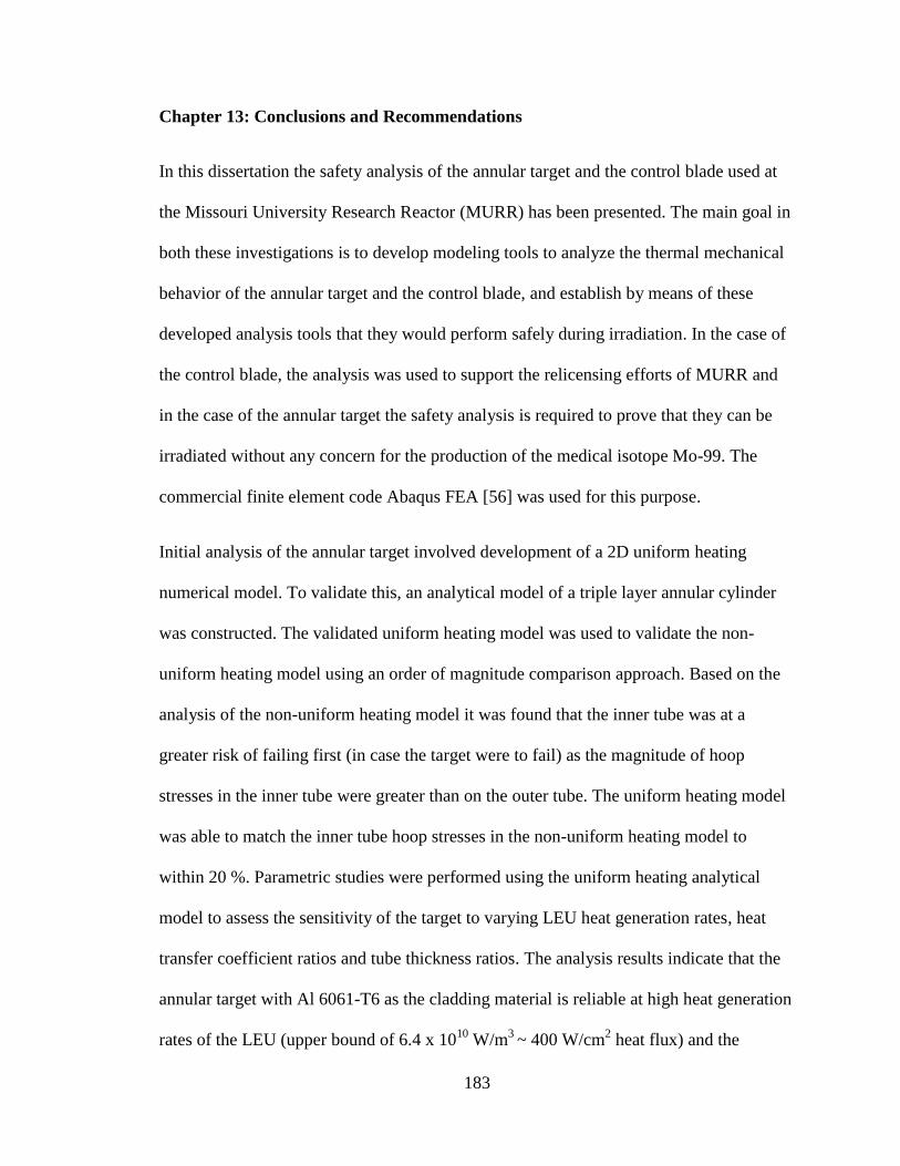
183

Chapter 13: Conclusions and Recommendations

In this dissertation the safety analysis of the annular target and the control blade used at

the Missouri University Research Reactor (MURR) has been presented. The main goal in

both these investigations is to develop modeling tools to analyze the thermal mechanical

behavior of the annular target and the control blade, and establish by means of these

developed analysis tools that they would perform safely during irradiation. In the case of

the control blade, the analysis was used to support the relicensing efforts of MURR and

in the case of the annular target the safety analysis is required to prove that they can be

irradiated without any concern for the production of the medical isotope Mo-99. The

commercial finite element code Abaqus FEA [56] was used for this purpose.

Initial analysis of the annular target involved development of a 2D uniform heating

numerical model. To validate this, an analytical model of a triple layer annular cylinder

was constructed. The validated uniform heating model was used to validate the non-

uniform heating model using an order of magnitude comparison approach. Based on the

analysis of the non-uniform heating model it was found that the inner tube was at a

greater risk of failing first (in case the target were to fail) as the magnitude of hoop

stresses in the inner tube were greater than on the outer tube. The uniform heating model

was able to match the inner tube hoop stresses in the non-uniform heating model to

within 20 %. Parametric studies were performed using the uniform heating analytical

model to assess the sensitivity of the target to varying LEU heat generation rates, heat

transfer coefficient ratios and tube thickness ratios. The analysis results indicate that the

annular target with Al 6061-T6 as the cladding material is reliable at high heat generation

rates of the LEU (upper bound of 6.4 x 1010

W/m3

~ 400 W/cm2 heat flux) and the

184

magnitude of separation can be controlled by adjusting the heat transfer coefficient split

between the inner and outer surfaces.

The second part of the annular target analysis involved inclusion of the assembly residual

stresses by simulating either the hydroforming or the draw-plug assembly process before

the irradiation analysis. A three step elasto-plastic model was built. In the hydroforming

analysis, the first analysis step simulated the hydroforming process using an internal

pressure of 36.4 MPa and this was followed by a pressure relaxation step to simulate the

recovery. In the axisymmetric draw-plug analysis, the first step simulated the draw-plug

assembly process by applying a velocity of 0.160726 m/s to the base of the plug. This

was followed by a step where the plug was removed from the simulation. Finally, in both

these analyses, the irradiation process was simulated by including the residual stresses

from the previous step. The results from the hydroforming and the draw-plug analysis

procedures indicate that the residual stresses from the assembly process tend to negate

and decrease the stresses at the end of the irradiation step. This is favorable from a

material standpoint as the inner and outer tubes are unlikely to fail under the applied heat

generation of 1.6 x 1010

W/m3. This corresponds to a heat flux of ~ 100 W/cm

2 incident

on the outer surface of the inner tube and the inner surface of the outer tube.

The effects of fission gas release, uranium swelling, thermal contact conductance, heat

generation in the cladding, and the pressure exerted by the coolant flow, were studied for

the draw-plug based irradiation model. The analysis results indicate very small changes

in temperatures and von Mises stresses for each of the cases considered in the analysis.

The group of parameters that provide the worst case scenarios for the temperatures and

von Mises stresses was found to be different. The combination of thermal contact

185

conductance, uranium swelling, fission gas pressure and the cladding heat generation

represent the worst case scenario for the temperatures, while this combination along with

the pressure exerted by the coolant represents the worst case scenario for the von Mises

stresses. The swelling of the uranium was found to have no significant impact on the

temperatures and von Mises stresses, while the fractional release based fission gas

pressure was found to have very small changes on the temperatures and the stresses.

The parametric study results showed that the maximum temperature even at the highest

heat generation rate is well within the melting temperature of the Al 6061-T6 cladding

material. While there is sufficient margin for the maximum cladding temperature at the

highest heat generation rate, the maximum von Mises stress nearly tends towards the

yield point of the cladding, providing a very narrow safety margin. However, it should be

noted that it is highly unlikely that this heat generation rate of 6.4 x 1010

W/m3 would be

attained during target irradiation as it represents an ‘over 100 % power’ scenario and the

reactor would be scrammed automatically or manually. Therefore, it can be concluded

that the annular target is thermally and structurally safe based on the parameters used in

the current analysis, and is unlikely to cause a safety concern.

For the BORAL control blades the task was to establish that the deflection of the blade

due to heating will be within the control blade channel gap of 6.5 mm. The BORAL meat

was split into 4 quadrants and a heat generation profile that varied with thickness and

longitudinal position was applied to each quadrant. The magnitude of the resulting

thermally induced deflection was found to be within the channel gap limit of 6.5 mm.

The heating profile showed some asymmetry in temperature and the corresponding

asymmetric deflection along the blade curvature has been discussed. Finally, thermal

186

conductivity parametric studies on the BORAL suggested that the maximum radial

deflection of the blade is still within the control blade channel gap limit even at a

BORAL thermal conductivity of 132 W/mK, which was considered to be the upper

bound in the thermal conductivity study.

Apart from providing an annular target performance analysis envelope, the ability to

successfully apply the developed tool set to other specific problems, such as the BORAL

control blade analysis to help with relicensing efforts and the HFIR safety case analysis

to support safe irradiation of targets, has also been demonstrated in this dissertation.

Analytical work has also been done, by developing a generalized dimensionless thermal-

stress model for a compound cylinder configuration. The work completed through the

course of this dissertation has been documented, presented in conferences, and published

in journals as well.

Recommendations for future work include extension of the dimensionless thermal stress

model to include the thermal contact conductance, and developing an experimental test

plan for the thermal contact conductance determination in a composite cylindrical

structure. As the determination of the surface parameters play a key role in accurate

experimental estimation of the thermal contact conductance, it is also recommended that

a test methodology to measure the surface roughness be developed.

187

APPENDIX

APPENDIX 1: Mathematica Code to Determine Heat Flux

Clear[r1,r2,r3,r4,Tinf,Kal,h1,h4,L,Rconvout,Rcondout,Rcondin,Rconvin,Reffout,Reffin,

REFF,quranium,qinward,qoutward,qfluxinward,qfluxoutward]

(*Rcondout,Rconvout,Reffout : conduction resistance through the outer aluminum tube ,

convective resistance on the outer tube outer surface and effective series resistance in the

radially outward direction *)

(*Rcondin,Rconvin,Reffin : conduction resistance through the inner aluminum tube ,

convective resistance on the inner tube inner surface and effective series resistance in the

radially inward direction *)

(* Dimensions and other definitions *)

r1=0.01321; (*meters*) (*Inner tube inner radius *)

r2= 0.013995;(*meters*) (* Inner tube outer radius = Foil Inner radius *)

r3= 0.01412; (*meters*)(* Foil outer radius =Outer tube Inner radius *)

r4=0.015075;(*meters*) (* Outer tube outer radius *)

foilthickness=125*10^-6;(*meters*)

rcenter=(r2+((r3-r2)/2)); (*meters*) (* Uranium foil center line radius *)

Tinf=323;(*Kelvin*)(* Coolant temperature *)

Kal=167; (*W/mK*)(* Thermal conductivity of Aluminum *)

Ku =27.5; (*W/mK*)(* Thermal conductivity of Uranium *)

h1 = 19000; (*W/m^2K*)(*Inner tube heat transfer coefficient *)

h4 = 19000;(*W/m^2K*)(*Outer tube heat transfer coefficient *)

L=0.100; (*meters*) (* length of the heated section which will be the length of the foil *)

(* Determination of uranium temperature *)

Rcondout= Log[r4/r3] / (2*Pi*Kal*L);(*Kelvin/Watt*) (* Conduction resistance in the

outer tube *)

Rconvout = 1/ (h4*2*Pi*r4*L);(*Kelvin/Watt*)(* Convective resistance outer coolant *)

Reffout=Rcondout+Rconvout;(*Kelvin/Watt*) (* Effective resistance of the outer tube *)

Rcondin= Log[r2/r1] / (2*Pi*Kal*L);(*Kelvin/Watt*)(* Conduction resistance in the

inner tube *)

Rconvin = 1/ (h1*2*Pi*r1*L);(*Kelvin/Watt*) (* Convective resistance inner coolant *)

188

Ruraniumin=Log[rcenter/r2]/(2*Pi*Ku*L);

Reffin =Rcondin+Rconvin(*+ Ruraniumin *);(*Kelvin/Watt*)

REFF = (Reffout*Reffin)/(Reffout+Reffin);(*Kelvin/Watt*) (* resistance in parallel *)

(*deltaT=Turanium-Tinf; (*Kelvin*) *)

quranium=17665.17 ; (*Watts*) (* obtain quranium from qgen =1.6*10^10 as follows :

quranium=qgen*2*Pi*rcenter*L*foilthickness *)

Turanium = Tinf + (REFF * quranium); (* Temperature of uranium *)

(* Now that the uranium temperature has been determined it can be used to calculate the

heat fluxes in the radially inward and outward directions *)

(* quranium = qoutward + qinward *)

qoutward = (Turanium-Tinf)/(Reffout) ;(*Watts*)

qfluxoutward=qoutward/(2*Pi*r3*L) ; (*W/m^2*)(* Radially outward heat flux *)

qinward=(Turanium-Tinf)/(Reffin) ; (*Watts*)

qfluxinward=qinward/(2*Pi*r2*L)(*W/m^2*) ; (* Radially inward heat flux *)

(*The heat fluxes obtained here are used to determine the analytical radial stress, hoop

stress , displacements and temperature*)

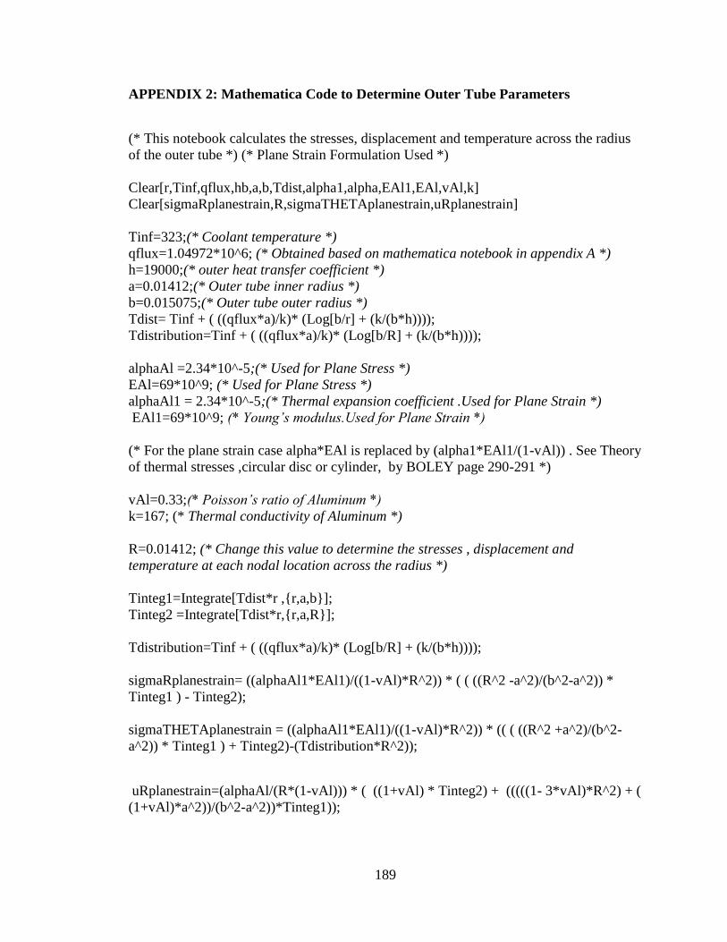
189

APPENDIX 2: Mathematica Code to Determine Outer Tube Parameters

(* This notebook calculates the stresses, displacement and temperature across the radius

of the outer tube *) (* Plane Strain Formulation Used *)

Clear[r,Tinf,qflux,hb,a,b,Tdist,alpha1,alpha,EAl1,EAl,vAl,k]

Clear[sigmaRplanestrain,R,sigmaTHETAplanestrain,uRplanestrain]

Tinf=323;(* Coolant temperature *)

qflux=1.04972*10^6; (* Obtained based on mathematica notebook in appendix A *)

h=19000;(* outer heat transfer coefficient *)

a=0.01412;(* Outer tube inner radius *)

b=0.015075;(* Outer tube outer radius *)

Tdist= Tinf + ( ((qflux*a)/k)* (Log[b/r] + (k/(b*h))));

Tdistribution=Tinf + ( ((qflux*a)/k)* (Log[b/R] + (k/(b*h))));

alphaAl =2.34*10^-5;(* Used for Plane Stress *)

EAl=69*10^9; (* Used for Plane Stress *)

alphaAl1 = 2.34*10^-5;(* Thermal expansion coefficient .Used for Plane Strain *)

EAl1=69*10^9; (* Young’s modulus.Used for Plane Strain *)

(* For the plane strain case alpha*EAl is replaced by (alpha1*EAl1/(1-vAl)) . See Theory

of thermal stresses ,circular disc or cylinder, by BOLEY page 290-291 *)

vAl=0.33;(* Poisson’s ratio of Aluminum *)

k=167; (* Thermal conductivity of Aluminum *)

R=0.01412; (* Change this value to determine the stresses , displacement and

temperature at each nodal location across the radius *)

Tinteg1=Integrate[Tdist*r ,{r,a,b}];

Tinteg2 =Integrate[Tdist*r,{r,a,R}];

Tdistribution=Tinf + ( ((qflux*a)/k)* (Log[b/R] + (k/(b*h))));

sigmaRplanestrain= ((alphaAl1*EAl1)/((1-vAl)*R^2)) * ( ( ((R^2 -a^2)/(b^2-a^2)) *

Tinteg1 ) - Tinteg2);

sigmaTHETAplanestrain = ((alphaAl1*EAl1)/((1-vAl)*R^2)) * (( ( ((R^2 +a^2)/(b^2-

a^2)) * Tinteg1 ) + Tinteg2)-(Tdistribution*R^2));

uRplanestrain=(alphaAl/(R*(1-vAl))) * ( ((1+vAl) * Tinteg2) + (((((1- 3*vAl)*R^2) + (

(1+vAl)*a^2))/(b^2-a^2))*Tinteg1));

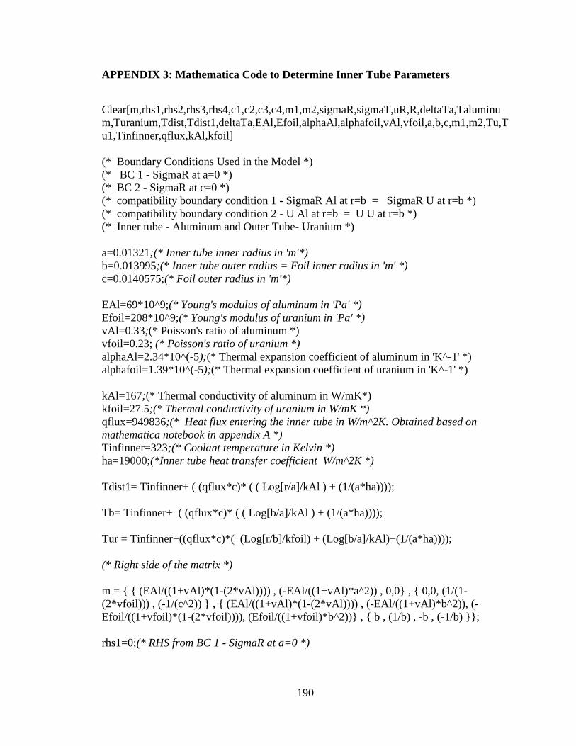
190

APPENDIX 3: Mathematica Code to Determine Inner Tube Parameters

Clear[m,rhs1,rhs2,rhs3,rhs4,c1,c2,c3,c4,m1,m2,sigmaR,sigmaT,uR,R,deltaTa,Taluminu

m,Turanium,Tdist,Tdist1,deltaTa,EAl,Efoil,alphaAl,alphafoil,vAl,vfoil,a,b,c,m1,m2,Tu,T

u1,Tinfinner,qflux,kAl,kfoil]

(* Boundary Conditions Used in the Model *)

(* BC 1 - SigmaR at a=0 *)

(* BC 2 - SigmaR at c=0 *)

(* compatibility boundary condition 1 - SigmaR Al at r=b = SigmaR U at r=b *)

(* compatibility boundary condition 2 - U Al at r=b = U U at r=b *)

(* Inner tube - Aluminum and Outer Tube- Uranium *)

a=0.01321;(* Inner tube inner radius in 'm'*)

b=0.013995;(* Inner tube outer radius = Foil inner radius in 'm' *)

c=0.0140575;(* Foil outer radius in 'm'*)

EAl=69*10^9;(* Young's modulus of aluminum in 'Pa' *)

Efoil=208*10^9;(* Young's modulus of uranium in 'Pa' *)

vAl=0.33;(* Poisson's ratio of aluminum *)

vfoil=0.23; (* Poisson's ratio of uranium *)

alphaAl=2.34*10^(-5);(* Thermal expansion coefficient of aluminum in 'K^-1' *)

alphafoil=1.39*10^(-5);(* Thermal expansion coefficient of uranium in 'K^-1' *)

kAl=167;(* Thermal conductivity of aluminum in W/mK*)

kfoil=27.5;(* Thermal conductivity of uranium in W/mK *)

qflux=949836;(* Heat flux entering the inner tube in W/m^2K. Obtained based on

mathematica notebook in appendix A *)

Tinfinner=323;(* Coolant temperature in Kelvin *)

ha=19000;(*Inner tube heat transfer coefficient W/m^2K *)

Tdist1= Tinfinner+ ( (qflux*c)* ( ( Log[r/a]/kAl ) + (1/(a*ha))));

Tb= Tinfinner+ ( (qflux*c)* ( ( Log[b/a]/kAl ) + (1/(a*ha))));

Tur = Tinfinner+((qflux*c)*( (Log[r/b]/kfoil) + (Log[b/a]/kAl)+(1/(a*ha))));

(* Right side of the matrix *)

m = { { (EAl/((1+vAl)*(1-(2*vAl)))) , (-EAl/((1+vAl)*a^2)) , 0,0} , { 0,0, (1/(1-

(2*vfoil))) , (-1/(c^2)) } , { (EAl/((1+vAl)*(1-(2*vAl)))) , (-EAl/((1+vAl)*b^2)), (-

Efoil/((1+vfoil)*(1-(2*vfoil)))), (Efoil/((1+vfoil)*b^2))} , { b , (1/b) , -b , (-1/b) }};

rhs1=0;(* RHS from BC 1 - SigmaR at a=0 *)

191

rhs2= ((alphafoil*(1+vfoil)) /((1-vfoil)* (c^2)))*Integrate[Tur*r,{r,a,c}];(* RHS from BC

2 - SigmaR at c=0 *)

rhs3= ((-alphafoil*Efoil / ((1-vfoil)*(b^2)))*Integrate[Tdist1*r,{r,a,b}])+((alphaAl*EAl /

((1-vAl)*(b^2)))*Integrate[Tb*r,{r,a,b}]); (* RHS from compatibility condition 1 -

SigmaR Al at r=b = SigmaR U at r=b *)

rhs4= (((1+vfoil)*alphafoil / ((1-vfoil)*(b)))*Integrate[Tdist1*r,{r,a,b}])+((-

(1+vAl)*alphaAl / ((1-vAl)*(b)))*Integrate[Tb*r,{r,a,b}]);(* RHS from compatibility

condition 2 - U Al at r=b=U U at r=b *)

(* Solving the matrix to determine the four constants *)

m1=c1; (* replace c1 with m1 just for convenience*)

m2=c2; (* replace c2 with m2 just for convenience*)

Clear[sigmaR,sigmaT,Tdist,R]

R=0.0132885;(* Change R to determine the stresses and temperature at any nodal

location across the radius of the tube *)

Tdist=Tinfinner+ ( (qflux*c)* ( ( Log[R/a]/kAl ) + (1/(a*ha))))

sigmaR = -(((alphaAl*EAl)/((1-vAl)*R^2))*Integrate[Tdist1*r ,{r,a,R}] )+ (

(EAl/(1+vAl))*( (m1/(1-(2*vAl)))-(m2/R^2)))

sigmaT = (((alphaAl*EAl)/((1-vAl)*R^2))*Integrate[ Tdist1*r,{r,a,R}])-

((alphaAl*EAl*Tdist)/(1-vAl))+ ( (EAl/(1+vAl))*( (m1/(1-(2*vAl)))+(m2/R^2)))

uRplanestrain = (( ((1+vAl)*alphaAl)/((1-vAl)*R))*Integrate[Tdist1*r,{r,a,R}]) +

(m11*R)+(m22/R)

192

APPENDIX 4: Mathematica Code to Determine Contact Pressure.

(* This mathematica notebook is to compare the pressure obtained using Abaqus to that

obtained using Madhusudhana's formulation *)

(* The obtained pressure will be in MPa *)

Clear[delTi,p,Ta]

a=13.21*10^(-3); (* Inner tube inner radius in 'm'*)

b=13.995*10^(-3); (* Inner tube outer radius = Foil inner radius in 'm' *)

c=14.12*10^(-3); (* Foil outer radius in 'm'*)

kAl=167; (* Thermal conductivity of aluminum in 'W/mK ' *)

alphaAl1=2.34*10^(-5);(* Thermal expansion coefficient of aluminum in ' W/mK ' *)

EAl1=70*10^9;(* Young's modulus of aluminum in 'Pa' *)

vAl1=0.33; (* Poisson's ratio of aluminum *)

kU=27.5; (* Thermal conductivity of uranium in 'W/mK ' *)

alphaU1=1.39*10^(-5);(* Thermal expansion coefficient of uranium in ' W/mK ' *)

EU1=208*10^9;(* Young's modulus of uranium in 'Pa' *)

vU1=0.23;(* Poisson's ratio of uranium *)

(* Writing E,v and alpha in terms of plane strain *)

Ei1=EAl1/(1-(vAl1^2));vi1=vAl1/(1-vAl1);alphai1=alphaAl1*(1+vAl1);ki=kAl;

E01=EU1/(1-(vU1^2));v01=vU1/(1-vU1);alpha01=alphaU1*(1+vU1);k0=kU;

uC=0.0; (* Initial interference in 'm' *)

h=10^9; (* Total contact conductance in 'W/m^2K '. A high value implies infinite

conductance and perfect contact *)

(*Ta- Temp at the inner surface of the inner tube *)

(*T1-Temp at the outer surface of the inner tube *)

delTi=Ta-T1; (* Temp rise in the inner tube *)

DELTAT = (ki*delTi )/((b*Log[b/a])*h); (* ie DELTAT= q/h where q=Q/A *)

c1=Ei1/E01;

c2=(c^2+b^2)/(c^2-b^2);

c3=(b^2+a^2)/(b^2-a^2);

(*delT0=(ki/k0)*delTi*(Log[c/b]/Log[b/a]);*)

uAi = (b*alphai1*delTi)* (1-( (2*a^2)/(b^2-a^2))*Log[b/a])/(2*Log[b/a]);

uA0 = (b*alphai1*delTi)* ((alpha01*ki)/(alphai1*k0))*( Log[c/b]/Log[b/a])* ( 1-(

(2*c^2)/(c^2-b^2))*Log[c/b]) / (2*Log[c/b]);

193

uA=uAi-uA0; (* Interference due to heat flux in ‘m’ *)

uB = b*(T1*(alphai1-alpha01) + (alphai1*DELTAT)); (* Interference due to contact

resistance in ‘m’*)

u=uA+uB+uC;(* Total interference in ‘m’ *)

(* Solving to obtain the contact pressure in MPa *)

Solve[u == ((b*p)/(Ei1))*(c1*(c2+v01)+(c3-vi1)),p]

194

APPENDIX 5: Mathematica Code to Calculate Fission Gas Pressure

(* This code calculates the fission gas pressure for the Al 6061-T6 model *)

Clear[T,Tc1,Tc2,Tc3,Vc1,Vc2,Vc3,w1,w2,w3,n1,n2,n3,ntotal,y1,y2,y3,Tr,B1,B2,B3,Bze

ro1,Bzero2,Bzero3,Bone1,Bone2,Bone3,Pc1,Pc2,Pc3,R,Zc1,Zc2,Zc3]

Clear[Tc11,Tc12,Tc13,Tc21,Tc22,Tc23,Tc31,Tc32,Tc33,Zc11,Zc12,Zc13,Zc21,Zc22,Zc

23,Zc31,Zc32,Zc33,Vc11,Vc12,Vc13,Vc21,Vc22,Vc23,Vc31,Vc32,Vc33]

Clear[w11,w12,w13,w21,w22,w23,w31,w32,w33,Pc11,Pc12,Pc13,Pc21,Pc22,Pc23,Pc31,

Pc32,Pc33,B11,B12,B13,B21,B22,B23,B31,B32,B33]

Clear[Bzero11,Bzero12,Bzero13,Bzero21,Bzero22,Bzero23,Bzero31,Bzero32,Bzero33,B

one11,Bone12,Bone13,Bone21,Bone22,Bone23,Bone31,Bone32,Bone33,Bmix,Zmix,Pfi

ssion,compressibilityfactor, Pfissiongas, volume, Prelease]

T=425; (* Actual system temperature *)

R=8.3144; (* J/mol K *)

volume= 2.315 *10^-7 ;

(* 1- Xenon ; 2- Krypton; 3- Helium*)

(* Critical temperature in Kelvin *)

Tc1=289.7;

Tc2=209.4;

Tc3=5.19;

(* Critical pressure in Pascal *)

Pc1=5840000;

Pc2=5500000;

Pc3=227000;

(* Critical Volume in m^3 /mol *)

Vc1 =0.0001184;

Vc2=0.0000912;

Vc3=0.0000574;

(* Eccentricity Factor *)

w1=0.008;

w2=0.005;

w3=-0.365;

(* Mole fraction yi. ni is the number of moles *)

n1=20*5.44* 10^-6;

n2=20*8.34 * 10^-7;

n3= 20*2.65 * 10^-12;

ntotal=n1+n2+n3;

y1=n1/ntotal;

y2=n2/ntotal;

y3=n3/ntotal;

195

(* Individual virial coefficients calculation *)

Bzero1=0.083- (0.422 / ( (T/Tc1)^1.6));

Bone1=0.139-( 0.172 / ((T/Tc1)^4.2));

Bzero2=0.083- (0.422 / ( (T/Tc2)^1.6));

Bone2=0.139-( 0.172 / ((T/Tc2)^4.2));

Bzero3=0.083- (0.422 / ( (T/Tc3)^1.6));

Bone3=0.139-( 0.172 / ((T/Tc3)^4.2));

B1=(((Bzero1 + (w1 * Bone1))*(R*Tc1)) /Pc1);

B2=(((Bzero2 + (w2 * Bone2))*(R*Tc2)) /Pc2);

B3=(((Bzero3+ (w3 * Bone3))*(R*Tc3)) /Pc3);

(* Individual component critical compressibility factor Zci *)

Zc1= (1 + ( B1/Vc1));

Zc2= (1 + ( B2/Vc2));

Zc3= (1 + ( B3/Vc3));

(* Mixing rules for 2 component interactions *)

Tc11= Sqrt[ Tc1 * Tc1];Tc12= Sqrt[ Tc1 * Tc2];Tc13= Sqrt[ Tc1 * Tc3];

Tc21=Sqrt[Tc2*Tc1];Tc22=Sqrt[Tc2*Tc2];Tc23=Sqrt[Tc2*Tc3];

Tc31=Sqrt[Tc3*Tc1];Tc32=Sqrt[Tc3*Tc2];Tc33=Sqrt[Tc3*Tc3];

Zc11=0.5*(Zc1+Zc1);Zc12=0.5*(Zc1+Zc2);Zc13=0.5*(Zc1+Zc3);



Vc11= (0.5*(((Vc1)^1/3)+((Vc1)^1/3)))^3 ; Vc12= (0.5*(((Vc1)^1/3)+((Vc2)^1/3)))^3 ;

Vc13= (0.5*(((Vc1)^1/3)+((Vc3)^1/3)))^3 ;

Vc21= (0.5*(((Vc2)^1/3)+((Vc1)^1/3)))^3 ; Vc22= (0.5*(((Vc2)^1/3)+((Vc2)^1/3)))^3 ;

Vc23= (0.5*(((Vc2)^1/3)+((Vc3)^1/3)))^3 ;

Vc31= (0.5*(((Vc3)^1/3)+((Vc1)^1/3)))^3 ; Vc32= (0.5*(((Vc3)^1/3)+((Vc2)^1/3)))^3 ;

Vc33= (0.5*(((Vc3)^1/3)+((Vc3)^1/3)))^3 ;

w11=0.5*(w1+w1); w12=0.5*(w1+w2);w13=0.5*(w1+w3);

w21=0.5*(w2+w1); w22=0.5*(w2+w2);w23=0.5*(w2+w3);

w31=0.5*(w3+w1); w32=0.5*(w3+w2);w33=0.5*(w3+w3);

Pc11 = (R* Zc11 * Tc11)/Vc11; Pc12 = (R* Zc12 * Tc12)/Vc12; Pc13 = (R* Zc13 *

Tc13)/Vc13;


Tc23)/Vc23;


Tc33)/Vc33;

196

(* Calculate Bij *)

Bzero11=0.083 - (0.422/(T/Tc11)^1.6);Bzero12=0.083 -

(0.422/(T/Tc12)^1.6);Bzero13=0.083 - (0.422/(T/Tc13)^1.6);

Bzero21=0.083 - (0.422/(T/Tc21)^1.6);Bzero22=0.083 -

(0.422/(T/Tc22)^1.6);Bzero23=0.083 - (0.422/(T/Tc23)^1.6);

Bzero31=0.083 - (0.422/(T/Tc31)^1.6);Bzero32=0.083 -

(0.422/(T/Tc32)^1.6);Bzero33=0.083 - (0.422/(T/Tc33)^1.6);

Bone11=0.139- (0.172/(T/Tc11)^4.2);Bone12=0.139-

(0.172/(T/Tc12)^4.2);Bone13=0.139- (0.172/(T/Tc13)^4.2);

Bone21=0.139- (0.172/(T/Tc21)^4.2);Bone22=0.139-

(0.172/(T/Tc22)^4.2);Bone23=0.139- (0.172/(T/Tc23)^4.2);

Bone31=0.139- (0.172/(T/Tc31)^4.2);Bone32=0.139-

(0.172/(T/Tc32)^4.2);Bone33=0.139- (0.172/(T/Tc33)^4.2);

B11 = ((Bzero11 + (w11 * Bone11))*(R * Tc11 ))/Pc11; B12 = ((Bzero12 + (w12 *

Bone12))*(R * Tc12 ))/Pc12;B13 = ((Bzero13 + (w13 * Bone13))*(R * Tc13 ))/Pc13;





Bmix = (B1 * y1^2)+(B2* y2^2)+ (B3 * y3^2) + (2*y1*y2*B12) +

(2*y1*y3*B13)+(2*y2*y3*B23);

(*Compressibility factor*)

Zmix = 1+ (Bmix/( (Vc1+Vc2+Vc3) ))

0.830825

(* 100 % gas release pressure *)

Pfissiongas= Zmix* ntotal *R*T / (volume)

(* Fractional gas release pressure *)

Prelease = Pfissiongas *(5/125)*(1-0.25)

47739.1

1.5913 106

197

APPENDIX 6: Mathematica Code to Develop a Thermal Conductance Model for Al

6061-T6 and Al 6061-T6 Interface.

Clear[mew_He,mew_Xe,mew_Kr,mew_I,Ms,Mg,Mg_He,Mg_Kr,Mg_Xe,Mg_I,Ts,T0,C

0,C1,g1,g2,g3,g4,alpha1,alpha2,alpha3,alpha4,gamma1,gamma2,gamma3,gamma4,kg1,k

g2,kg3,kg4,visc1,visc2,visc3,visc4,cv1,cv2,cv3,cv4,lambda1,lambda2,lambda3,lambda4,

gm,bt,sigma,X,Y,deltaeff,phi11,phi12,phi13,phi14,phi21,phi22,phi23,phi24,phi31,phi32,

phi33,phi34,phi41,phi42,phi43,phi44,kgmix,x1,x2,x2,x3,k1,k2,k3,k4,hgmix,CLAsigmaN

i,CLAsigmaU,kNi,kU,ENi,EU,slopeNi,slopeU,vNi,vU,keff,sigmaeff,tantheta,Eeff,si,hs,P

,htotal,delta, CLAsigmaAl, CLAsigmaU, kAl, kU,EAl,EU,slopeAl,slopeU,vAl,vU]

(* --------------------------------------------------------------------------------------------*)

(* Mg and Ms - Molecular weight of gas and solid respectively in 'g/mol'*)

(* mew - ratio of molecular weights *)

(* alpha - accomodation coefficient *)

(* Ts and T0 - Temp of the solid and reference temp respectively *)

(* g and gm - Temperature jump distance for an individual component and a mixture

respectively *)

(* visc - dynamic viscosity *)

(* kg - thermal conductivity of the individual gas in W/mK *)

(* lambda - mean free path in 'm'*)

(* sigma - surface roughness *)

(* deltaeff - effective gap thickness = delta+2gm *)

(* kgmix - thermal conductivity of the gas mixture in W/mK*)

(* x and y - mass fraction and mole fraction respectively *)

(* gamma - ratio of specific heats *)

(* cv - specific heat at constant volume in J/Kg K *)

(* --------------------------------------------------------------------------------------------*)

(* Input values *)

(* 1- Helium; 2- Xenon ; 3- Krypton; *)

Ms=26.981538 *10^-3 ; (* Al *)

Mg1=3.017*10^-3;

Mg2=131.293*10^-3;

Mg3=83.8*10^-3;(* Kg/mol *)

visc1=21.7*10^-6;

visc2=26.17*10^-6;

visc3=28.6*10^-6; (* Kg/m s *)

kg1=0.1696;

kg2=0.00625;

kg3=0.01067; (* W/m K*)

198

gamma1=1.667;gamma2=1.656;gamma3=1.667;

cv1=3120;cv2=97;cv3=151; (* J/Kg K *)

lambda1=0.19266*10^-6;lambda2=0.03788*10^-6;lambda3=0.05234*10^-6; (* meter *)

y1=4.22378*10^-7;y2=0.86707;y3=0.132929;

x1=Mg1/(Mg1+Mg2+Mg3);x2=Mg2/(Mg1+Mg2+Mg3);x3=Mg3/(Mg1+Mg2+Mg3);

H=1080*10^6; (*Pa Hardness of Al the softer material obtained from *)

bt=6*sigma;

CLAsigmaAl=1*10^-6;

slopeAl=0.18; (*rad*)

kAl=167;

EAl=68.9*10^9;

vAl=0.33;


(*Accomodation coefficients from literature *)

alpha1=0.53;alpha2=0.86;alpha3=0.861;

(* Temperature jump distance calculation *)

g1=((2-alpha1)/alpha1)*( 2/(gamma1+1))*( kg1/(visc1*cv1))*lambda1;



gm =

((x1*g1/(Mg1^0.5))+(x2*g2/(Mg2^0.5))+(x3*g3/(Mg3^0.5)))/((x1/(Mg1^0.5))+(x2/(Mg

2^0.5))+(x3/(Mg3^0.5)))

(* Gap thickness calculation *)

X= bt/ (2*gm);

Y= 1/(0.305+(1/X));

deltaeff = (X/Y)*(2*gm);

(* Thermal conductivity of a mixture calculation using Wilke’s mixture rule*)

phi11=1;phi22=1;phi33=1;phi44=1;

phi12=(( 1+(visc1/visc2)^0.5 ( Mg2/Mg1)^0.25)^2)/( Sqrt[8]*( 1+(Mg1/Mg2))^0.5);


1.78288 107

199





kgmix = ( y1*kg1 / ((y1*phi11) + (y2*phi12)+ (y3*phi13) ))+ ( y2*kg2 / ((y1*phi21) +

(y2*phi22)+ (y3*phi23) ))+ ( y3*kg3 / ((y1*phi31) +(y2*phi32)+ (y3*phi33) ));

hgmix= FullSimplify[kgmix/(delta + (2*gm)) ](* W/m2 K *)

(* Solid spot conductance Calculations *)

keff= 2*kAl*kAl/(kAl+kAl);

sigmaeff=1.25* Sqrt[ CLAsigmaAl^2 + CLAsigmaAl^2];

tantheta= Sqrt[ slopeAl^2 + slopeAl^2];

Eeff = 2*(( ((1-vAl^2)/EAl)+ ((1-vAl^2)/EAl))^-1);

si= (Eeff/H)*tantheta

18.2245

(* plasticity index 'si' > 1 =>Mikic's correlation can be used for plastic deformation of

asperities *)

hs= 1.13* (keff/ (H^0.94))*(tantheta/sigmaeff)* (P^0.94)

(* Total conductance Calculations *)

htotal=FullSimplify[ Factor[hs + hgmix], P>0]

0.00672368

3.56575 10 7 delta

0.0876474 P0.94

0.00672368

3.56575 10 7 1. delta0.0876474 P

0.94

200


6061-T6 and Nickel Interface.







,htotal,delta, CLAsigmaAl,CLAsigmaU,kAl,kU,EAl,EU,slopeAl,slopeU,vAl,vU]

(* --------------------------------------------------------------------------------------------*)






respectively *)










(* --------------------------------------------------------------------------------------------*)

(* Input values *)


Ms=26.981538 *10^-3 ; (* Al *)

Mg1=3.017*10^-3;

Mg2=131.293*10^-3;

Mg3=83.8*10^-3;(* Kg/mol *)

visc1=21.7*10^-6;visc2=26.17*10^-6;visc3=28.6*10^-6; (* Kg/m s *)

kg1=0.1696;kg2=0.00625;kg3=0.01067; (* W/m K*)


cv1=3120;cv2=97;cv3=151; (* J/Kg K *)

201


y1=4.22378*10^-7;y2=0.86707;y3=0.132929;


H=1080*10^6; (*Pa Hardness of Al the softer material *)

bt=6*sigma;

CLAsigmaNi=1.27*10^-6;CLAsigmaAl=1.15*10^-6;

slopeNi=0.137; (*rad*)slopeAl=0.18; (*rad*) (* Nickel slope from Antonetti and

Yovanovich Table 1 *)

kNi=60.7;kAl=167;

ENi=207*10^9;EAl=68.9*10^9;

vNi=0.31;vAl=0.33;








gm =


2^0.5))+(x3/(Mg3^0.5)))


X= bt/ (2*gm);

Y= 1/(0.305+(1/X));

deltaeff = (X/Y)*(2*gm);


phi11=1;phi22=1;phi33=1;phi44=1;




1.78288 107

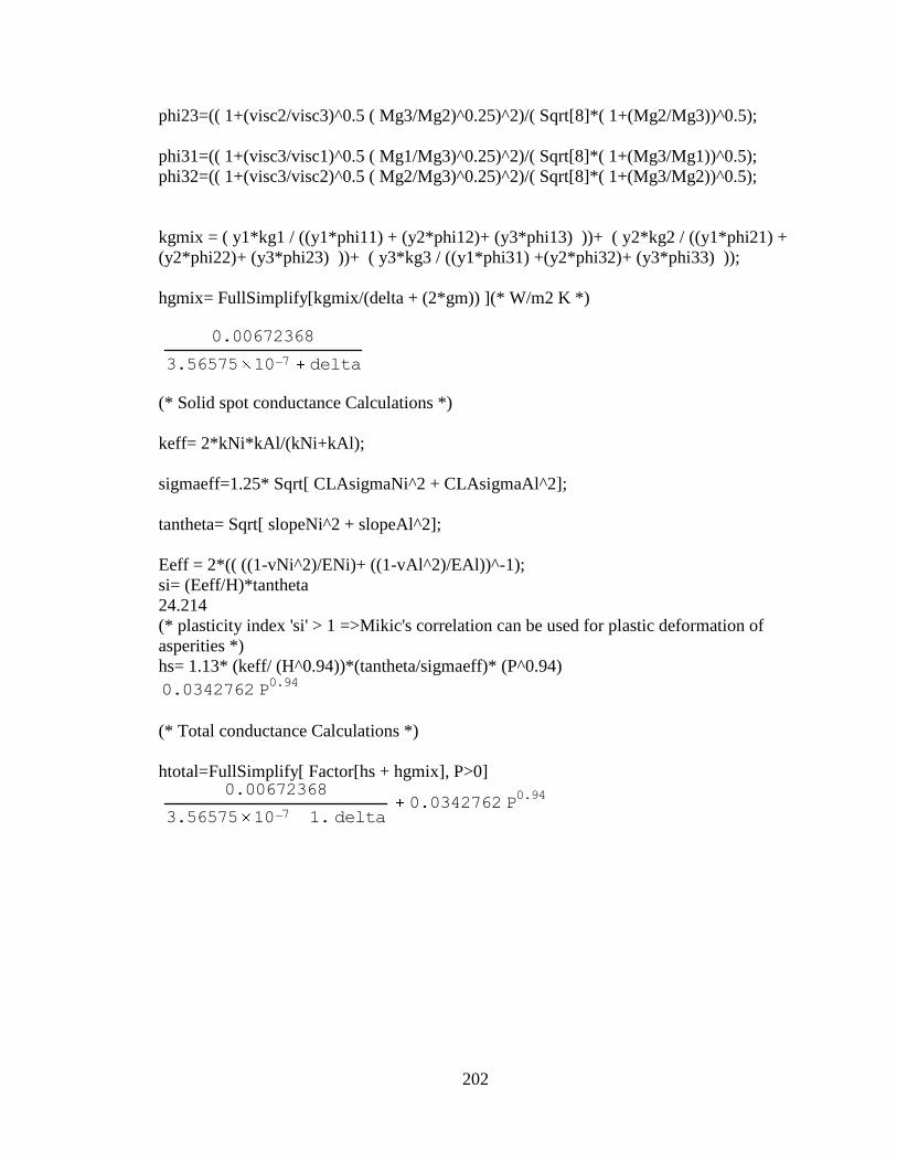
202








keff= 2*kNi*kAl/(kNi+kAl);

sigmaeff=1.25* Sqrt[ CLAsigmaNi^2 + CLAsigmaAl^2];

tantheta= Sqrt[ slopeNi^2 + slopeAl^2];

Eeff = 2*(( ((1-vNi^2)/ENi)+ ((1-vAl^2)/EAl))^-1);


24.214


asperities *)




0.00672368

3.56575 10 7 delta

0.0342762 P0.94

0.00672368

3.56575 10 7 1. delta0.0342762 P

0.94

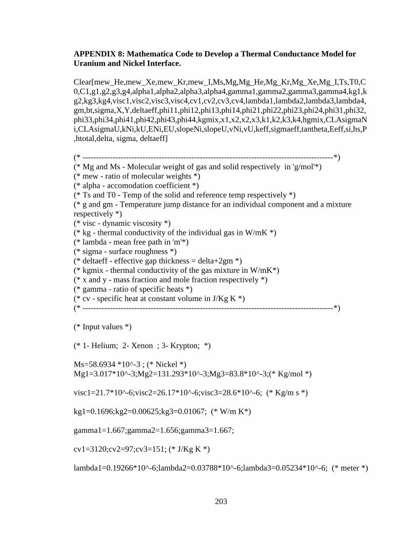
203

APPENDIX 8: Mathematica Code to Develop a Thermal Conductance Model for

Uranium and Nickel Interface.







,htotal,delta, sigma, deltaeff]

(* --------------------------------------------------------------------------------------------*)






respectively *)










(* --------------------------------------------------------------------------------------------*)

(* Input values *)


Ms=58.6934 *10^-3 ; (* Nickel *)

Mg1=3.017*10^-3;Mg2=131.293*10^-3;Mg3=83.8*10^-3;(* Kg/mol *)

visc1=21.7*10^-6;visc2=26.17*10^-6;visc3=28.6*10^-6; (* Kg/m s *)

kg1=0.1696;kg2=0.00625;kg3=0.01067; (* W/m K*)


cv1=3120;cv2=97;cv3=151; (* J/Kg K *)


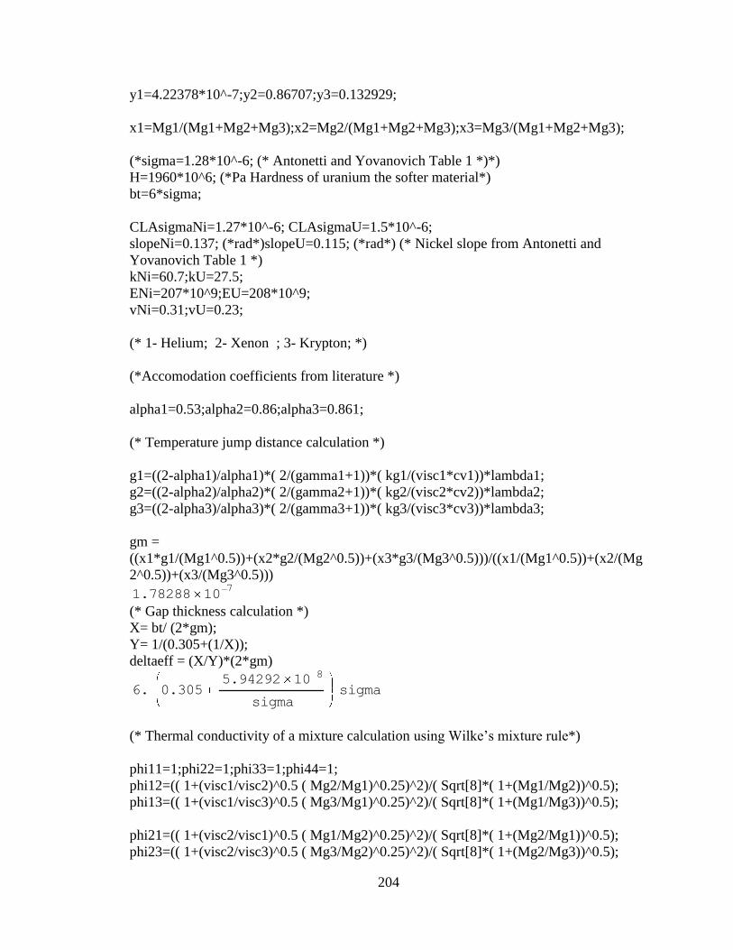
204

y1=4.22378*10^-7;y2=0.86707;y3=0.132929;


(*sigma=1.28*10^-6; (* Antonetti and Yovanovich Table 1 *)*)

H=1960*10^6; (*Pa Hardness of uranium the softer material*)

bt=6*sigma;

CLAsigmaNi=1.27*10^-6; CLAsigmaU=1.5*10^-6;

slopeNi=0.137; (*rad*)slopeU=0.115; (*rad*) (* Nickel slope from Antonetti and

Yovanovich Table 1 *)

kNi=60.7;kU=27.5;

ENi=207*10^9;EU=208*10^9;

vNi=0.31;vU=0.23;








gm =


2^0.5))+(x3/(Mg3^0.5)))


X= bt/ (2*gm);

Y= 1/(0.305+(1/X));

deltaeff = (X/Y)*(2*gm)


phi11=1;phi22=1;phi33=1;phi44=1;





1.78288 107

6. 0.3055.94292 10

8

sigmasigma

205







keff= 2*kNi*kU/(kNi+kU);

sigmaeff=1.25* Sqrt[ CLAsigmaNi^2 + CLAsigmaU^2];

tantheta= Sqrt[ slopeNi^2 + slopeU^2];

Eeff = 2*(( ((1-vNi^2)/ENi)+ ((1-vU^2)/EU))^-1);


20.4617


asperities *)




0.00672368

3.56575 10 7 delta

0.00573599 P0.94

0.00672368

3.56575 10 7 1. delta0.00573599 P

0.94

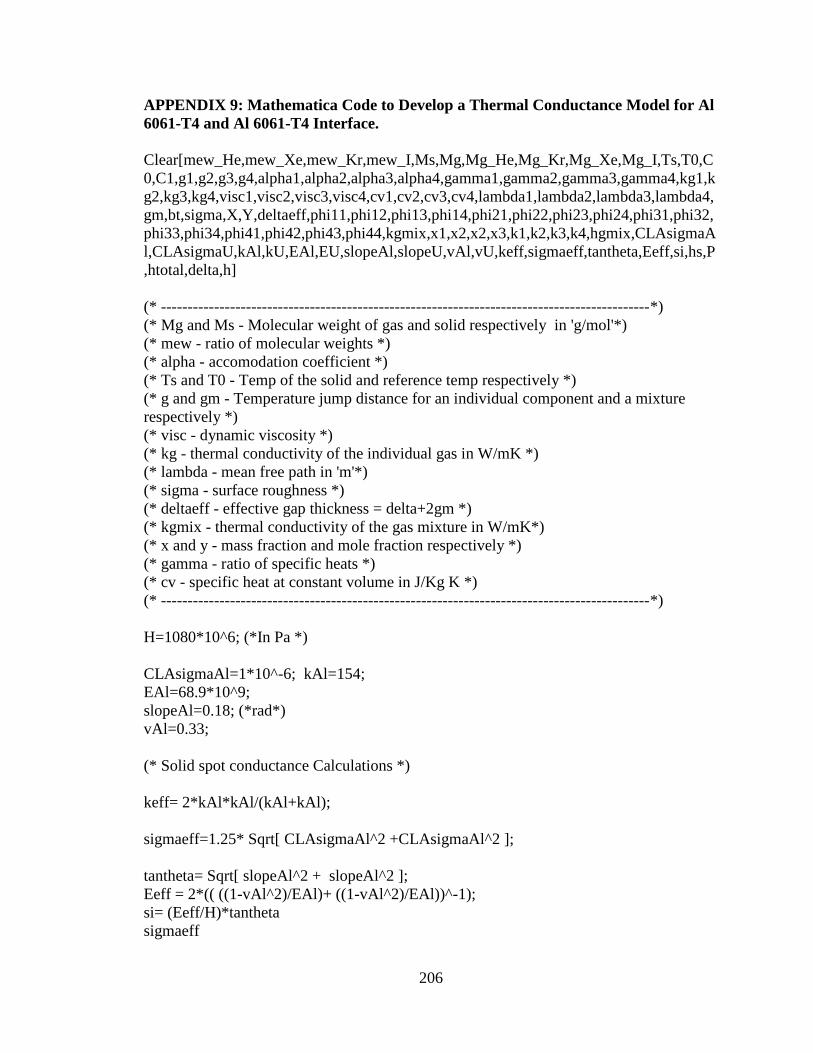
206


6061-T4 and Al 6061-T4 Interface.





phi33,phi34,phi41,phi42,phi43,phi44,kgmix,x1,x2,x2,x3,k1,k2,k3,k4,hgmix,CLAsigmaA

l,CLAsigmaU,kAl,kU,EAl,EU,slopeAl,slopeU,vAl,vU,keff,sigmaeff,tantheta,Eeff,si,hs,P

,htotal,delta,h]

(* --------------------------------------------------------------------------------------------*)






respectively *)










(* --------------------------------------------------------------------------------------------*)

H=1080*10^6; (*In Pa *)

CLAsigmaAl=1*10^-6; kAl=154;

EAl=68.9*10^9;

slopeAl=0.18; (*rad*)

vAl=0.33;


keff= 2*kAl*kAl/(kAl+kAl);

sigmaeff=1.25* Sqrt[ CLAsigmaAl^2 +CLAsigmaAl^2 ];

tantheta= Sqrt[ slopeAl^2 + slopeAl^2 ];

Eeff = 2*(( ((1-vAl^2)/EAl)+ ((1-vAl^2)/EAl))^-1);


sigmaeff

207


asperities *)


(* Input values For Gap Conductance Model *)

(* 1- Helium; 2- Xenon ; 3- Krypton; 4- Iodine *)

Ms=26.981538 *10^-3 ;Mg1=4.003*10^-3;Mg2=131.293*10^-3;Mg3=83.8*10^-

3;Mg4=253.809*10^-3; (* Kg/mol *)

visc1=21.7*10^-6; visc2=26.17*10^-6; visc3=28.6*10^-6; visc4= 23*10^-6; (* Kg/m s

*)

kg1=0.1696; kg2=0.00625; kg3=0.01067; kg4=0.449; (* W/m K*)

gamma1=1.667;gamma2=1.656;gamma3=1.667;gamma4=1.299;

cv1=3120;cv2=97;cv3=151;cv4=226.016; (* J/Kg K *)

lambda1=0.19266*10^-6; lambda2=0.03788*10^-6; lambda3=0.05234*10^-6;

lambda4=0.0419*10^-6; (* meter *)

y1=8.56*10^-5; y2=0.8146; y3=0.1136; y4=0.0705;

x1=Mg1/(Mg1+Mg2+Mg3+Mg4);





bt=6*sigmaeff;

alpha1=0.53;alpha2=0.86;alpha3=0.861;alpha4=0.73;






1.76777 106

0.0808246 P0.94

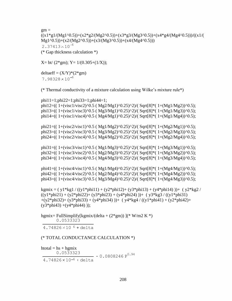
208

gm =

((x1*g1/(Mg1^0.5))+(x2*g2/(Mg2^0.5))+(x3*g3/(Mg3^0.5))+(x4*g4/(Mg4^0.5)))/((x1/(

Mg1^0.5))+(x2/(Mg2^0.5))+(x3/(Mg3^0.5))+(x4/(Mg4^0.5)))


X= bt/ (2*gm); Y= 1/(0.305+(1/X));



phi11=1;phi22=1;phi33=1;phi44=1;













kgmix = ( y1*kg1 / ((y1*phi11) + (y2*phi12)+ (y3*phi13) + (y4*phi14) ))+ ( y2*kg2 /

((y1*phi21) + (y2*phi22)+ (y3*phi23) + (y4*phi24) ))+ ( y3*kg3 / ((y1*phi31)

+(y2*phi32)+ (y3*phi33) + (y4*phi34) ))+ ( y4*kg4 / ((y1*phi41) + (y2*phi42)+

(y3*phi43) +(y4*phi44) ));


(* TOTAL CONDUCTANCE CALCULATION *)

htotal = hs + hgmix

2.37413 106

7.98328 106

0.0533323

4.74826 10 6 delta

0.0533323

4.74826 10 6 delta0.0808246 P

0.94

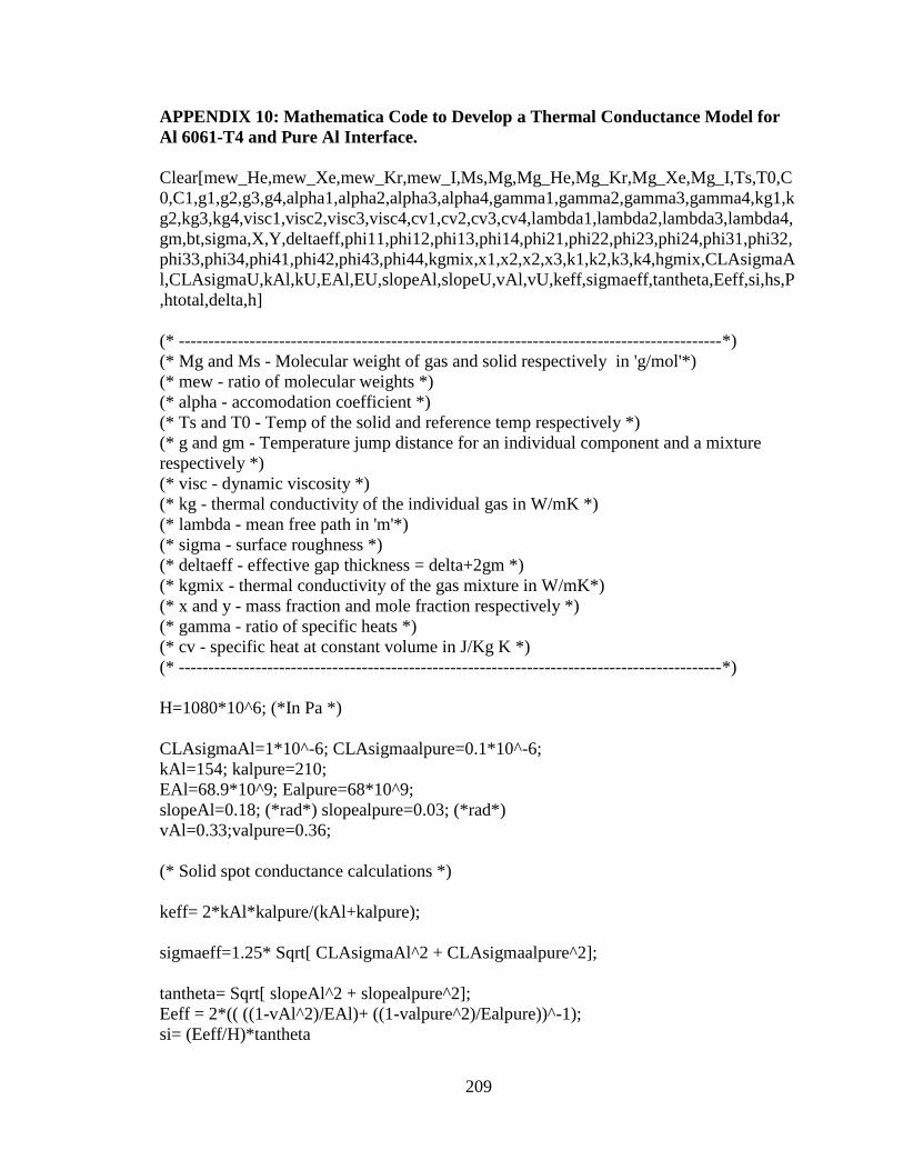
209

APPENDIX 10: Mathematica Code to Develop a Thermal Conductance Model for

Al 6061-T4 and Pure Al Interface.





phi33,phi34,phi41,phi42,phi43,phi44,kgmix,x1,x2,x2,x3,k1,k2,k3,k4,hgmix,CLAsigmaA

l,CLAsigmaU,kAl,kU,EAl,EU,slopeAl,slopeU,vAl,vU,keff,sigmaeff,tantheta,Eeff,si,hs,P

,htotal,delta,h]

(* --------------------------------------------------------------------------------------------*)






respectively *)










(* --------------------------------------------------------------------------------------------*)

H=1080*10^6; (*In Pa *)

CLAsigmaAl=1*10^-6; CLAsigmaalpure=0.1*10^-6;

kAl=154; kalpure=210;

EAl=68.9*10^9; Ealpure=68*10^9;

slopeAl=0.18; (*rad*) slopealpure=0.03; (*rad*)

vAl=0.33;valpure=0.36;

(* Solid spot conductance calculations *)

keff= 2*kAl*kalpure/(kAl+kalpure);

sigmaeff=1.25* Sqrt[ CLAsigmaAl^2 + CLAsigmaalpure^2];

tantheta= Sqrt[ slopeAl^2 + slopealpure^2];

Eeff = 2*(( ((1-vAl^2)/EAl)+ ((1-valpure^2)/Ealpure))^-1);


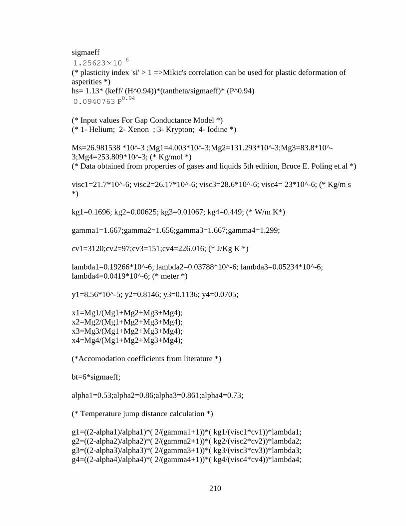
210

sigmaeff


asperities *)


(* Input values For Gap Conductance Model *)

(* 1- Helium; 2- Xenon ; 3- Krypton; 4- Iodine *)

Ms=26.981538 *10^-3 ;Mg1=4.003*10^-3;Mg2=131.293*10^-3;Mg3=83.8*10^-

3;Mg4=253.809*10^-3; (* Kg/mol *)

(* Data obtained from properties of gases and liquids 5th edition, Bruce E. Poling et.al *)

visc1=21.7*10^-6; visc2=26.17*10^-6; visc3=28.6*10^-6; visc4= 23*10^-6; (* Kg/m s

*)

kg1=0.1696; kg2=0.00625; kg3=0.01067; kg4=0.449; (* W/m K*)

gamma1=1.667;gamma2=1.656;gamma3=1.667;gamma4=1.299;

cv1=3120;cv2=97;cv3=151;cv4=226.016; (* J/Kg K *)

lambda1=0.19266*10^-6; lambda2=0.03788*10^-6; lambda3=0.05234*10^-6;

lambda4=0.0419*10^-6; (* meter *)

y1=8.56*10^-5; y2=0.8146; y3=0.1136; y4=0.0705;






bt=6*sigmaeff;

alpha1=0.53;alpha2=0.86;alpha3=0.861;alpha4=0.73;






1.25623 106

0.0940763 P0.94

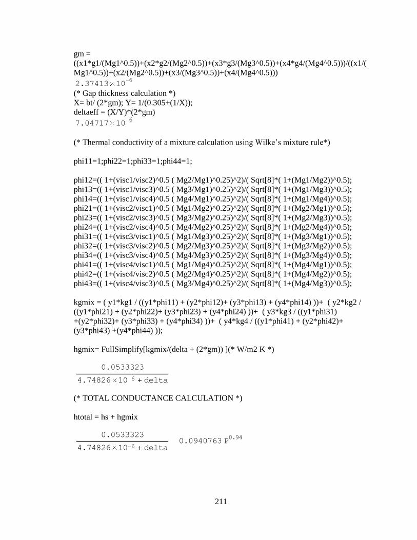
211

gm =

((x1*g1/(Mg1^0.5))+(x2*g2/(Mg2^0.5))+(x3*g3/(Mg3^0.5))+(x4*g4/(Mg4^0.5)))/((x1/(

Mg1^0.5))+(x2/(Mg2^0.5))+(x3/(Mg3^0.5))+(x4/(Mg4^0.5)))


X= bt/ (2*gm); Y= 1/(0.305+(1/X));



phi11=1;phi22=1;phi33=1;phi44=1;













kgmix = ( y1*kg1 / ((y1*phi11) + (y2*phi12)+ (y3*phi13) + (y4*phi14) ))+ ( y2*kg2 /

((y1*phi21) + (y2*phi22)+ (y3*phi23) + (y4*phi24) ))+ ( y3*kg3 / ((y1*phi31)

+(y2*phi32)+ (y3*phi33) + (y4*phi34) ))+ ( y4*kg4 / ((y1*phi41) + (y2*phi42)+

(y3*phi43) +(y4*phi44) ));


(* TOTAL CONDUCTANCE CALCULATION *)

htotal = hs + hgmix

2.37413 106

7.04717 106

0.0533323

4.74826 10 6 delta

0.0533323

4.74826 10 6 delta0.0940763 P

0.94

212

APPENDIX 11: Abaqus Input File for the Planar Model with Non-Uniform Heating

(The part and the mesh definitions have been omitted to make the presentation of the

code concise in this appendix. The description of the part creation along with the mesh

information has been provided in the dissertation write-up)

(To run the input file from the command window: abaqus job=**(the name of inp file,

without ".inp". To open the input file in the CAE environment: import the model. File

Import Model. This dialog will accept *.inp files)

*Heading

** Job name: FINEMESH-1 Model name: Model-1

** Generated by: Abaqus/CAE 6.10-2

*Preprint, echo=NO, model=NO, history=NO

**

**

** MATERIALS

**

*Material, name=al

*Conductivity

167.,

*Density

2700.,

*Elastic

6.9e+10, 0.33

*Expansion

2.34e-05,

*Specific Heat

963.,

*Material, name=uranium

*Conductivity

27.5,

*Density

19100.,

*Elastic

2.08e+11, 0.23

*Expansion

1.39e-05,

*Specific Heat

120.,

**

** INTERACTION PROPERTIES

**

*Surface Interaction, name=IntProp-1

1.,

*Friction

213

0.,

*Surface Behavior, pressure-overclosure=HARD

*Gap Conductance

1e+09, 0.

0., 0.1

**

** INTERACTIONS

**

** Interaction: IT-FOIL

*Contact Pair, interaction=IntProp-1, type=SURFACE TO SURFACE

_PickedSurf373, _PickedSurf372

** Interaction: OT-FOIL



** Interaction: it-ot



** ----------------------------------------------------------------

**

** STEP: Step-1

**

*Step, name=Step-1, nlgeom=YES

*Coupled Temperature-displacement, creep=none, steady state

1., 1., 1e-07, 1.

**

** BOUNDARY CONDITIONS

**

** Name: XSymm Type: Symmetry/Antisymmetry/Encastre

*Boundary

_PickedSet378, XSYMM

**

** LOADS

**

** Name: foil heat gen Type: Body heat flux

*Dflux

_PickedSet371, BF, 1.6e+10

**

** INTERACTIONS

**

** Contact Controls for Interaction: IT-FOIL

*Contact Controls, master=_PickedSurf372, slave=_PickedSurf373, stabilize=1.

** Contact Controls for Interaction: OT-FOIL


** Contact Controls for Interaction: it-ot


** Interaction: htc-inner

214

*Sfilm

_PickedSurf369, F, 323., 19000.

** Interaction: htc-outer

*Sfilm

_PickedSurf370, F, 323., 19000.

**

** OUTPUT REQUESTS

**

*Restart, write, frequency=0

**

** FIELD OUTPUT: F-Output-1

**

*Output, field, variable=PRESELECT

**

** HISTORY OUTPUT: H-Output-1

**

*Output, history, variable=PRESELECT

*End Step

215

APPENDIX 12: Abaqus Input File for the Hydroforming and Irradiation Model







*Heading

** Job name: Ar1 Model name: Ar



**

** PARTS

**

*Part, name=foil

*Node

(* foil part definitions omitted to maintain brevity *)

*Element, type=CPE8RT

(* element definitions omitted to maintain brevity *)

*Nset, nset=Set-2, generate

(* include node definitions here*)

*Elset, elset=Set-2, generate

(* include element set numbers/definitions here *)

*Elset, elset=_foil-inner_S4, internal


*Elset, elset=_foil-inner_S2, internal


*Surface, type=ELEMENT, name=foil-inner

(* include selected surface definitions here *)

*Elset, elset=_foil-outer_S2, internal


*Elset, elset=_foil-outer_S4, internal


*Surface, type=ELEMENT, name=foil-outer


** Section: foil

*Solid Section, elset=Set-2, material=uranium-plastic

*End Part

**

*Part, name="inner tube"

*Node

(* part definitions omitted to maintain brevity *)


216



(* include node set numbers/definitions here *)



*Elset, elset=_IT-inner_S4, internal


*Elset, elset=_IT-inner_S2, internal


*Surface, type=ELEMENT, name=IT-inner


*Elset, elset=_IT-outer_S2, internal


*Elset, elset=_IT-outer_S4, internal


*Surface, type=ELEMENT, name=IT-outer


** Section: inner tube

*Solid Section, elset=Set-2, material=Al6061-Plastic

*End Part

**

*Part, name="outer tube"

*Node

(* part definitions omitted to maintain brevity *)




(* include node set numbers/definitions here *)



*Elset, elset=_OT-outer_S2, internal


*Elset, elset=_OT-outer_S4, internal


*Surface, type=ELEMENT, name=OT-outer


*Elset, elset=_OT-inner_S4, internal


*Elset, elset=_OT-inner_S2, internal


*Surface, type=ELEMENT, name=OT-inner


** Section: outer tube

*Solid Section, elset=Set-3, material=Al6061-Plastic

*End Part

**

217

**

** ASSEMBLY

**

*Assembly, name=Assembly

**

*Instance, name="inner tube-1", part="inner tube"

*End Instance

**

*Instance, name=foil-1, part=foil

*End Instance

**

*Instance, name="outer tube-1", part="outer tube"

*End Instance

**

*Nset, nset=Set-1, instance="inner tube-1"

*Nset, nset=Set-1, instance=foil-1

*Nset, nset=Set-1, instance="outer tube-1"









*Nset, nset=Set-5, instance="inner tube-1", generate

*Nset, nset=Set-5, instance=foil-1, generate

*Nset, nset=Set-5, instance="outer tube-1", generate

*Elset, elset=Set-5, instance="inner tube-1", generate

*Elset, elset=Set-5, instance=foil-1, generate

*Elset, elset=Set-5, instance="outer tube-1", generate













*Elset, elset=_m_Surf-1_S4, internal, instance="inner tube-1", generate


*Surface, type=ELEMENT, name=m_Surf-1

218

*Elset, elset=_s_Surf-1_S2, internal, instance="outer tube-1", generate


*Surface, type=ELEMENT, name=s_Surf-1

*Elset, elset=_Surf-3_S2, internal, instance="outer tube-1"




*Surface, type=ELEMENT, name=Surf-3

*Elset, elset=_Surf-4_S4, internal, instance="inner tube-1"
















*Elset, elset=_m_Surf-8_S4, internal, instance=foil-1





*Elset, elset=_s_Surf-8_S2, internal, instance="inner tube-1"










*Elset, elset=_s_Surf-10_S4, internal, instance="outer tube-1"







219













































*End Assembly

**

220

** MATERIALS

**

*Material, name=Al6061-Plastic

*Conductivity

167.,

*Density

2700.,

*Elastic

6.89e+10, 0.33

*Expansion

2.34e-05,

*Plastic

2.97854e+08, 0.

3.03817e+08, 0.000103788

3.12636e+08, 0.000203785

3.14828e+08, 0.000303384

3.18827e+08, 0.000466394

3.20234e+08, 0.000552785

3.21799e+08, 0.000608999

3.22592e+08, 0.000731266

3.23178e+08, 0.000858794

3.23667e+08, 0.000971875

3.24081e+08, 0.00108532

3.28852e+08, 0.00200756

3.29762e+08, 0.00204261

3.30583e+08, 0.00401162

3.31514e+08, 0.00511611

3.32279e+08, 0.00602954

3.33093e+08, 0.00701644

3.33968e+08, 0.008079

3.34803e+08, 0.00909294

3.35637e+08, 0.0101208

3.36457e+08, 0.011144

3.37167e+08, 0.0120147

3.38029e+08, 0.0130966

3.38808e+08, 0.0140844

3.39581e+08, 0.0150898

3.40346e+08, 0.0160675

3.41153e+08, 0.0171126

3.4187e+08, 0.0180507

3.42642e+08, 0.0190953

3.43421e+08, 0.0201244

3.47061e+08, 0.0250944

3.50529e+08, 0.030057

3.53853e+08, 0.0350468

3.57066e+08, 0.0401315

221

3.59996e+08, 0.0450281

3.62781e+08, 0.0500108

3.65415e+08, 0.0550523

3.67808e+08, 0.0600356

3.70049e+08, 0.0651016

3.72034e+08, 0.070092

3.73799e+08, 0.0750486

3.75406e+08, 0.0800535

3.77033e+08, 0.0853327

3.78426e+08, 0.0900701

3.79805e+08, 0.0950171

3.81142e+08, 0.100062

3.92367e+08, 0.157004

4.02426e+08, 0.223144

4.11107e+08, 0.300105

4.20111e+08, 0.405465

4.26544e+08, 0.500775

4.31495e+08, 0.587787

4.32908e+08, 0.615186

4.36645e+08, 0.693147

4.37748e+08, 0.71784

4.40713e+08, 0.788457

4.41609e+08, 0.81093

4.44795e+08, 0.896088

4.45512e+08, 0.916291

4.48697e+08, 1.0116

*Material, name=uranium-plastic

*Conductivity

27.5,

*Density

19100.,

*Elastic

2.06327e+11, 0.23

*Expansion

1.39e-05,

*Plastic

1.11e+08, 0.

2.32e+08, 0.001

2.99e+08, 0.003

3.36e+08, 0.005

3.63e+08, 0.007

3.94e+08, 0.01

**


**

*Surface Interaction, name=contact-assembly

222

1.,

*Friction

0.,

*Surface Behavior, no separation, pressure-overclosure=HARD

*Gap Conductance

1e+09, 0.

0., 0.01

*Surface Interaction, name=contact-irrad

1.,

*Friction

0.,


*Gap Conductance

1e+09, 0.

0., 0.01

**

** INTERACTIONS

**

** Interaction: IT-OT

*Contact Pair, interaction=contact-assembly, type=SURFACE TO SURFACE

s_Surf-1, m_Surf-1

** Interaction: Inner-Foil-Irradiation

*Contact Pair, interaction=contact-irrad, type=SURFACE TO SURFACE

s_Surf-14, m_Surf-14

** Interaction: Inner-Outer-Irradiation



** Interaction: Outer-Foil-Irradiation



** Interaction: foil-innertube


"inner tube-1".IT-outer, foil-1.foil-inner

** Interaction: foil-outertube


"outer tube-1".OT-inner, foil-1.foil-outer

** ----------------------------------------------------------------

**

** STEP: Coupled-assembly

**

*Step, name=Coupled-assembly, nlgeom=YES, inc=1000


1., 1., 1e-09, 1.

**


**

223

** Name: xSymm Type: Symmetry/Antisymmetry/Encastre

*Boundary

Set-1, XSYMM

** Name: xsymm2 Type: Symmetry/Antisymmetry/Encastre

*Boundary

Set-2, XSYMM

** Name: ysymm1 Type: Symmetry/Antisymmetry/Encastre

*Boundary

Set-8, YSYMM

** Name: ysymm2 Type: Symmetry/Antisymmetry/Encastre

*Boundary

Set-9, YSYMM

**

** LOADS

**

** Name: internal pressure Type: Pressure

*Dsload

"inner tube-1".IT-inner, P, 3.6e+07

**

** INTERACTIONS

**

** Contact Controls for Interaction: IT-OT

*Contact Controls, master=m_Surf-1, slave=s_Surf-1, stabilize=1.


*Model Change, type=CONTACT PAIR, remove








** Contact Controls for Interaction: foil-innertube

*Contact Controls, master=foil-1.foil-inner, slave="inner tube-1".IT-outer, stabilize=1.

** Contact Controls for Interaction: foil-outertube

*Contact Controls, master=foil-1.foil-outer, slave="outer tube-1".OT-inner, stabilize=1.

**

** OUTPUT REQUESTS

**


**


**

*Output, field

*Node Output

CF, NT, RF, RFL, U

224

*Element Output, directions=YES

E, HFL, LE, PE, PEEQ, PEMAG, S, THE

*Contact Output

CDISP, CSTRESS

**


**


*End Step

** ----------------------------------------------------------------

**

** STEP: Relieve Pressure

**

*Step, name="Relieve Pressure", nlgeom=YES


1., 1., 1e-05, 1.

**

** LOADS

**

** Name: internal pressure Type: Pressure

*Dsload, op=NEW

**

** OUTPUT REQUESTS

**


**


**

*Output, field

*Node Output

CF, NT, RF, RFL, U



*Contact Output

CDISP, CSTRESS

**


**


*End Step

** ----------------------------------------------------------------

**

** STEP: Irradiation

**

*Step, name=Irradiation, nlgeom=YES


225

1., 1., 1e-09, 1.

**

** LOADS

**

** Name: HEAT GEN Type: Body heat flux

*Dflux

Set-10, BF, 1.6e+10

**

** INTERACTIONS

**

** Interaction: IT-OT


s_Surf-1, m_Surf-1


*Model Change, type=CONTACT PAIR, add


** Contact Controls for Interaction: Inner-Foil-Irradiation





** Contact Controls for Interaction: Inner-Outer-Irradiation





** Contact Controls for Interaction: Outer-Foil-Irradiation


** Interaction: foil-innertube


"inner tube-1".IT-outer, foil-1.foil-inner

** Interaction: foil-outertube


"outer tube-1".OT-inner, foil-1.foil-outer

** Interaction: InnerHTC

*Sfilm

Surf-20, F, 323., 19000.

** Interaction: OuterHTC

*Sfilm

Surf-21, F, 323., 19000.

**

** OUTPUT REQUESTS

**


**


226

**

*Output, field

*Node Output

CF, NT, RF, RFL, U



*Contact Output

CDISP, CSTRESS

**


**


*End Step

227

APPENDIX 13: Abaqus Input File for the Draw-Plug Based Irradiation Model







*Heading

** Job name: interf-1 Model name: interf


*Heading

** Job name: interf-1 Model name: interf



**

** PARTS

**

*Part, name="Ni foil"

*Node


*Element, type=CAX4RT






** Section: Nickel

*Solid Section, elset=Set-15, material=Nickel

*End Part

**

*Part, name=foil

*Node








*Elset, elset="_foil inner_S2", internal, generate

*Surface, type=ELEMENT, name="foil inner"

*Elset, elset="_foil outer_S4", internal, generate

*Surface, type=ELEMENT, name="foil outer"

228

** Section: Uranium

*Solid Section, elset=Set-24, material=URANIUM

*End Part

**

*Part, name=innertube

*Node




*Nset, nset=Set-1


2101, 3600, 1


1, 4149, 1


1, 3900, 1

*Elset, elset=_INNERcoolant_S3, internal

*Elset, elset=_INNERcoolant_S2, internal, generate

*Surface, type=ELEMENT, name=INNERcoolant

*Elset, elset="_recess reg- inner_S4", internal, generate

*Surface, type=ELEMENT, name="recess reg- inner"

*Elset, elset=_upper_S3, internal, generate

3851, 3900, 1

*Surface, type=ELEMENT, name=upper

_upper_S3, S3

*Elset, elset=_lower_S3, internal, generate

3701, 3750, 1

*Surface, type=ELEMENT, name=lower

** Section: Al6061-T6

*Solid Section, elset=Set-60, material=Al6061-T6

*End Part

**

*Part, name=outertube

*Node




*Elset, elset=Set-14


1, 4305, 1


1, 4080, 1

*Elset, elset="_recess reg-inner_S2", internal, generate

1000, 1040, 20

*Elset, elset="_recess reg-inner_S4", internal, generate

1041, 4001, 20

229

*Surface, type=ELEMENT, name="recess reg-inner"

*Elset, elset="_recess reg- outer_S4", internal, generate

*Elset, elset="_recess reg- outer_S2", internal, generate

*Surface, type=ELEMENT, name="recess reg- outer"

*Elset, elset=_upper-inner_S2, internal, generate

*Elset, elset=_upper-inner_S4, internal, generate

*Surface, type=ELEMENT, name=upper-inner

*Elset, elset=_OUTERcoolant_S4, internal, generate

*Elset, elset=_OUTERcoolant_S2, internal, generate

*Surface, type=ELEMENT, name=OUTERcoolant

** Section: Al6061-T6

*Solid Section, elset=Set-21, material=Al6061-T6

*End Part

**

*Part, name=plug1048

*Node





1, 395, 1


1, 357, 1

*Nset, nset=Set-9

*Elset, elset=Set-9



** Section: Plug

*Solid Section, elset=Set-12, material="D2 STEEL"

*End Part

**

**

** ASSEMBLY

**

*Assembly, name=Assembly

**

*Instance, name=innertube-1, part=innertube

*End Instance

**

*Instance, name="Ni foil-1", part="Ni foil"

*End Instance

**

*Instance, name=foil-1, part=foil

*End Instance

**

*Instance, name=outertube-1, part=outertube

230

*End Instance

**

*Instance, name=plug1048-1, part=plug1048

*End Instance

**

*Nset, nset=Set-74, instance=innertube-1

*Nset, nset=Set-74, instance=outertube-1

*Nset, nset=s_Set-76, instance=innertube-1



*Nset, nset=Set-78, instance=plug1048-1

*Elset, elset=Set-78, instance=plug1048-1




*Elset, elset=Set-80, instance=plug1048-1, generate

*Nset, nset=Set-81, instance=plug1048-1, generate


*Nset, nset=Set-82, instance=innertube-1

*Nset, nset=Set-82, instance=outertube-1

*Elset, elset=Set-82, instance=innertube-1

*Elset, elset=Set-82, instance=outertube-1, generate

*Nset, nset=s_Set-83, instance=innertube-1

*Nset, nset=Set-84, instance="Ni foil-1", generate


*Elset, elset=Set-84, instance="Ni foil-1", generate




*Nset, nset=Set-98, instance=plug1048-1, generate










*Nset, nset=Set-103, instance=innertube-1, generate

*Elset, elset=Set-103, instance=innertube-1, generate

*Nset, nset=Set-104, instance=outertube-1, generate

*Elset, elset=Set-104, instance=outertube-1, generate

*Elset, elset=_s_Surf-76_S3, internal, instance=innertube-1

*Elset, elset=_s_Surf-76_S2, internal, instance=innertube-1, generate


231

*Elset, elset=_m_Surf-78_S2, internal, instance=innertube-1



*Elset, elset=_s_Surf-78_S4, internal, instance="Ni foil-1"




*Elset, elset=_m_Surf-80_S2, internal, instance="Ni foil-1", generate

*Elset, elset=_m_Surf-80_S4, internal, instance="Ni foil-1"


*Elset, elset=_s_Surf-80_S1, internal, instance=foil-1, generate




*Elset, elset=_m_Surf-82_S4, internal, instance=foil-1, generate


*Elset, elset=_s_Surf-82_S2, internal, instance="Ni foil-1", generate





*Elset, elset=_s_Surf-84_S4, internal, instance=outertube-1, generate


*Elset, elset=_m_Surf-86_S3, internal, instance=innertube-1, generate























232








*Elset, elset=_m_Surf-103_S2, internal, instance=outertube-1, generate







































233




*Elset, elset=_Surf-121_S3, internal, instance=innertube-1

*Elset, elset=_Surf-121_S2, internal, instance=innertube-1, generate


*Elset, elset=_Surf-122_S4, internal, instance=outertube-1, generate



*Elset, elset=_m_Surf-123_S2, internal, instance=plug1048-1, generate
















*Elset, elset=_m_Surf-129_S4, internal, instance=outertube-1, generate





















234











*Elset, elset=_Surf-142_S2, internal, instance=innertube-1, generate





*Surface, type=NODE, name=s_Set-76_CNS_, internal

*Surface, type=NODE, name=s_Set-83_CNS_, internal

*End Assembly

*Amplitude, name=AMP-1, definition=SMOOTH STEP

0., 0., 0.001, 1., 1., 1.

**

** MATERIALS

**

*Material, name=Al6061-T6

*Conductivity

167.,

*Density

2700.,

*Elastic

6.89e+10, 0.33

*Expansion

2.36e-05,

*Plastic

2.97854e+08, 0.

3.03817e+08, 0.000104

3.12636e+08, 0.000204

3.14828e+08, 0.000303

3.18827e+08, 0.000466

3.20234e+08, 0.000553

3.21799e+08, 0.000609

3.22592e+08, 0.000731

3.23178e+08, 0.000859

3.23667e+08, 0.000972

3.24081e+08, 0.00109

3.28852e+08, 0.00201

3.29762e+08, 0.00204

235

3.30583e+08, 0.00401

3.31514e+08, 0.00512

3.32279e+08, 0.00603

3.33093e+08, 0.00702

3.33968e+08, 0.00808

3.34803e+08, 0.00909

3.35637e+08, 0.0101

3.36457e+08, 0.0111

3.37167e+08, 0.012

3.38029e+08, 0.0131

3.38808e+08, 0.0141

3.39581e+08, 0.0151

3.40346e+08, 0.0161

3.41153e+08, 0.0171

3.4187e+08, 0.0181

3.42642e+08, 0.0191

3.43421e+08, 0.0201

3.47061e+08, 0.0251

3.50529e+08, 0.0301

3.53853e+08, 0.035

3.57066e+08, 0.0401

3.59996e+08, 0.045

3.62781e+08, 0.05

3.65415e+08, 0.0551

3.67808e+08, 0.06

3.70049e+08, 0.0651

3.72034e+08, 0.0701

3.73799e+08, 0.075

3.75406e+08, 0.0801

3.77033e+08, 0.0853

3.78426e+08, 0.0901

3.79805e+08, 0.095

3.81142e+08, 0.1

3.92367e+08, 0.157

4.02426e+08, 0.223

4.11107e+08, 0.3

4.20111e+08, 0.405

4.26544e+08, 0.501

4.31495e+08, 0.588

4.32908e+08, 0.615

4.36645e+08, 0.693

4.37748e+08, 0.718

4.40713e+08, 0.788

4.41609e+08, 0.811

4.44795e+08, 0.896

4.45512e+08, 0.916

236

4.48697e+08, 1.01

*Material, name="D2 STEEL"

*Conductivity

20.,

*Density

7700.,

*Elastic

2.1e+11, 0.3

*Material, name=Nickel

*Conductivity

60.7,

*Density

8800.,

*Elastic

2.07e+11, 0.31

*Expansion

1.31e-05,

*Material, name=URANIUM

*Conductivity

27.5,

*Density

19050.,

*Elastic

2.08e+11, 0.23

*Expansion

1.39e-05,

*Plastic

1.11e+08, 0.

2.32e+08, 0.001

2.99e+08, 0.003

3.36e+08, 0.005

3.63e+08, 0.007

3.94e+08, 0.01

*Swelling

2.48e-08,

**


**

*Surface Interaction, name=INTPROP-1

1.,

*Friction

0.,


*Gap Conductance

1e+09, 0.

0., 0.01

237

*Surface Interaction, name=IRRAD

1.,

*Friction

0.,


*Gap Conductance

1e+09, 0.

0., 0.01

*Surface Interaction, name="IRRAD-Aluminum Aluminum"

1.,

*Friction

0.,


*Gap Conductance

18790.1, 0.

4938.93, 1e-06

646.93, 1e-05

66.76, 0.0001

6.7, 0.001

0.67, 0.01

0.07, 0.1

0., 1.

*Gap Conductance, pressure

18790.1, 0.

18796.8, 100.

18848., 1000.

19294.2, 10000.

23180.5,100000.

57028.9, 1e+06

351836., 1e+07

2.9195e+06, 1e+08

*Surface Interaction, name="IRRAD-Aluminum Ni"

1.,

*Friction

0.,


*Gap Conductance

18790.1, 0.

4938.93, 1e-06

646.93, 1e-05

66.76, 0.0001

6.7, 0.001

0.67, 0.01

0.07, 0.1

0., 1.


238

18790.1, 0.

18792.9, 100.

18814.1, 1000.

18999., 10000.

20609.5,100000.

34635.7, 1e+06

156799., 1e+07

1.2208e+06, 1e+08

*Surface Interaction, name="IRRAD-Ni Uranium"

1.,

*Friction

0.,


*Gap Conductance

18790.1, 0.

4938.93, 1e-06

646.93, 1e-05

66.76, 0.0001

6.7, 0.001

0.67, 0.01

0.07, 0.1

0., 1.


18790.1, 0.

18790.6, 100.

18793.9, 1000.

18822.9, 10000.

19075.8,100000.

21278.3, 1e+06

40460.9, 1e+07

207535., 1e+08

*Surface Interaction, name=WELD

1.,

*Friction

0.,


*Gap Conductance

1e+09, 0.

0., 0.01

**

** INTERACTIONS

**

** Interaction: IRRAD-innertube-nickel

*Contact Pair, interaction="IRRAD-Aluminum Ni", type=SURFACE TO SURFACE


** Interaction: IRRAD-it-ot-base

239

*Contact Pair, interaction="IRRAD-Aluminum Aluminum", type=SURFACE TO

SURFACE


** Interaction: IRRAD-it-ot-top

*Contact Pair, interaction="IRRAD-Aluminum Aluminum", type=SURFACE TO

SURFACE


** Interaction: IRRAD-nickel-outertube

*Contact Pair, interaction="IRRAD-Aluminum Ni", type=SURFACE TO SURFACE


** Interaction: IRRAD-uranium-nickel-2

*Contact Pair, interaction="IRRAD-Ni Uranium", type=SURFACE TO SURFACE


** Interaction: MP-innertube-nickel

*Contact Pair, interaction=INTPROP-1, type=SURFACE TO SURFACE


** Interaction: MP-innertube-nickel-base



** Interaction: MP-innertube-nickel-top



** Interaction: MP-it-ot-base



** Interaction: MP-it-ot-top



** Interaction: MP-nickel-outertube



** Interaction: MP-nickel-uranium-1



** Interaction: MP-plug-innertube



** Interaction: MP-uranium-nickel-2



** Interaction: RP-it-ot-base



** Interaction: RP-it-ot-base-weld

*Contact Pair, interaction=WELD, type=SURFACE TO SURFACE

s_Set-76_CNS_, m_Surf-103

240

** Interaction: RP-it-ot-top



** Interaction: RP-it-ot-top-weld

*Contact Pair, interaction=WELD, type=SURFACE TO SURFACE


** ----------------------------------------------------------------

**

** STEP: Move plug

**

*Step, name="Move plug", nlgeom=YES, inc=10000


0.001, 1., 1e-12, 1.

**


**

** Name: Plug velocity Type: Velocity/Angular velocity

*Boundary, amplitude=AMP-1, type=VELOCITY

Set-99, 2, 2, 0.160726

** Name: U2 zero Type: Displacement/Rotation

*Boundary

Set-82, 2, 2

** Name: Vel1-Zero Type: Velocity/Angular velocity


Set-102, 1, 1

** Name: Vel3-Zero Type: Velocity/Angular velocity


Set-101, 6, 6

**

** INTERACTIONS

**
















241













**

** OUTPUT REQUESTS

**


**


**

*Output, field

*Node Output

CF, NT, RF, RFL, U


CFAILURE, DAMAGEC, DAMAGEFC, DAMAGEFT, DAMAGEMC, DAMAGEMT,

DAMAGESHR, DAMAGET, DMICRT, E, EE, ERPRATIO, HFL, HSNFCCRT,

HSNFTCRT, HSNMCCRT

HSNMTCRT, JK, LE, PE, PEEQ, PEMAG, S, SDEG, SHRRATIO, THE

*Contact Output

BDSTAT, CDISP, CRSTS, CSDMG, CSMAXSCRT, CSMAXUCRT, CSQUADSCRT,

CSQUADUCRT, CSTRESS, DBS, DBSF, DBT, EFENRRTR, ENRRT, OPENBC

**


**


*End Step

** ----------------------------------------------------------------

**

** STEP: Remove Plug and Weld

**

*Step, name="Remove Plug and Weld", nlgeom=YES


1., 1., 1e-05, 1.

**


**

** Name: Plug velocity Type: Velocity/Angular velocity

242


Set-99, 2, 2

**

** INTERACTIONS

**

** Interaction: MP-it-ot-base



** Interaction: MP-it-ot-top



** Interaction: RP- Remove Plug

*Model Change, remove

Set-98,













**

** OUTPUT REQUESTS

**


**


**

*Output, field

*Node Output

CF, NT, RF, RFL, U




HSNFTCRT, HSNMCCRT


*Contact Output



**


243

**


*End Step

** ----------------------------------------------------------------

**

** STEP: Irrad

**

*Step, name=Irrad, nlgeom=YES, inc=100000


1., 1., 1e-12, 1.

**

** LOADS

**

** Name: CHG-inner Type: Body heat flux

*Dflux

Set-103, BF, 2.7e+07

** Name: CHG-outer Type: Body heat flux

*Dflux

Set-104, BF, 2.7e+07

** Name: CP- inner tube inner surf Type: Pressure

*Dsload

Surf-142, P, 590000.

** Name: CP-outer tube outer surf Type: Pressure

*Dsload

Surf-143, P, 590000.

** Name: FGP Type: Pressure

*Dsload

Surf-141, P, 47740.

** Name: heat gen Type: Body heat flux

*Dflux

Set-85, BF, 1.6e+10

**

** INTERACTIONS

**




** Contact Controls for Interaction: IRRAD-innertube-nickel





** Contact Controls for Interaction: IRRAD-it-ot-base




244


** Contact Controls for Interaction: IRRAD-it-ot-top





** Contact Controls for Interaction: IRRAD-nickel-outertube





** Contact Controls for Interaction: IRRAD-uranium-nickel-2


** Interaction: MP-innertube-nickel



** Interaction: MP-innertube-nickel-base



** Interaction: MP-innertube-nickel-top



** Interaction: MP-nickel-outertube



** Interaction: MP-nickel-uranium-1



** Interaction: MP-plug-innertube



** Interaction: MP-uranium-nickel-2









** Interaction: IRRAD-HTC in

*Sfilm

Surf-121, F, 323., 19000.

** Interaction: IRRAD-HTCout

*Sfilm

Surf-122, F, 323., 19000.

245

**

** OUTPUT REQUESTS

**


**


**

*Output, field

*Node Output

CF, NT, RF, RFL, U




HSNFTCRT, HSNMCCRT


*Contact Output



**


**


*End Step

246

APPENDIX 14: Abaqus Input File for the Control Blade Analysis







*Heading

** Job name: U1U30PROFILEBK98 Model name: U1U30PROFILEBK98



**

** PARTS

** (* part definition omitted in this section to make the code concise and clear *)

**

** MATERIALS

**

*Material, name=Al1100

*Conductivity

186.4,

*Density

2713.,

*Elastic

6.9e+10, 0.33

*Expansion

2.36e-05,

*Specific Heat

1120.,

*Material, name=boral

*Conductivity

98.,

*Density

2481.,

*Elastic

6.2053e+10, 0.23

*Expansion

1.97e-05,

*Specific Heat

1380.,

**


**

*Surface Interaction, name=IntProp-1

247

1.,

*Friction

0.,


*Gap Conductance

1e+09, 0.

0., 0.1

**

** INTERACTIONS

**

** Interaction: gc

*Contact

*Contact Inclusions, ALL EXTERIOR

*Contact Property Assignment

, , IntProp-1

*Surface Property Assignment, property=GEOMETRIC CORRECTION

**

** STEP: Step-1

**

*Step, name=Step-1, nlgeom=YES


1., 1., 1e-05, 1.

**


**

** Name: BC-1 Type: Displacement/Rotation

*Boundary

_PickedSet1184, 1, 1



*Boundary




*Boundary




*Boundary




*Boundary




248

*Boundary




*Boundary




*Boundary




*Boundary




*Boundary



**

** LOADS

**

** Name: LEFT EDGE Type: Body heat flux Using Field: LEFT EDGE

*Dflux, op=NEW (* check chapter 12 for the body flux equation definition *)

**

** INTERACTIONS

**

** Interaction: htc1

*Sfilm

_PickedSurf933, F, 325., 1000.

** Interaction: htc2

*Sfilm

_PickedSurf934, F, 325., 1000.

**

** OUTPUT REQUESTS

**


**


**

*Output, field, variable=PRESELECT

**


**


*End Step

249

REFERENCES

1. S.M. Seidlin, L.D. Marinelli, E. Oshry, “Radioactive Iodine Therapy: Effect on

Functioning Metastases of Adenocarcinoma of Thyroid,” JAMA, 132, pp. 838-

847, 1946.

2. A. Georges, O. Bersillion, J. Blachot, A.H. Wapstra, “The NUBASE Evaluation

of Nuclear and Decay Properties,” Nuclear Physics A (Atomic Mass Data Center),

729, pp. 3-128, 2003.

3. E. Segre, C.S.Wu, “Some Fission Products of Uranium,” Physical Review, 57 (6),

pp. 552-552, 1940.

4. L. Sorensen, M. Archambault, “Visualization of the Liver by Scanning with Mo-

99 (Molybdate) as tracer,” Journal of Laboratory and Clinical Medicine, 62, pp.

330-340, 1963.

5. C.W. Allen, R.A. Butler, C.A. Jarousse, J.L. Falgoux, “Feasibility Development

Program, LEU Foil Plate Target for the Production of Molybdenum-99,” RERTR

International Meeting, Prague, Czech Republic, 2007.

6. G.F. Vandegrift, C. Conner, G.L. Hofman, R.A. Leonard, A. Mutalib, J. Sedlet,

D.E. Walker, T.C. Wiencek, J.L. Snelgrove, “Modification of Targets and

Processes for Conversion of Mo-99 Production from High- to Low-Enriched

Uranium,” Industrial and Engineering Chemistry. Research, 39, pp. 3140-3145,

2000.

7. J.A. Smaga, J. Sedlet, C. Conner, M.W. Liberatore, D.E. Walker, D.G. Wygmans,

G.F. Vandegrift, “ Electroplating Fission Recoil Barriers onto LEU Metal Foils

for Mo-99 Production Targets,” Proceedings of the XXth International Meeting

250

on Reduced Enrichment for Research and Test Reactors, Jackson Hole, WY,

1997.

8. K.K. Turner, “The Thermal-Mechanical Analysis of Targets for the High Volume

Production of Molybdenum-99 Using a Low-Enriched Uranium Metal Foil [PhD

Dissertation],” University of Missouri, Columbia, MO, 2012.

9. National Research Council, 2009, Medical Isotope Production Without Highly

Enriched Uranium, The National Academies Press, Washington, D.C.

10. C.V. Madhusudhana, Thermal Contact Conductance, Springer, New York, NY,

1996.

11. US. Department of Energy, DOE Fundamentals Handbook- Nuclear Physics and

Reactor Theory, 2, pp. 48-58, 1993.

12. Missouri University Research Reactor, User’s Guide- University of Missouri

Research Reactor Facility, Columbia, MO, 1969.

13. C. Conner, E.F. Lewandowski, J.L. Snelgrove, M.W. Liberatore, D.E. Walker,

T.C. Wiencek, D.J. McGrann, G.L. Hofman, G.F. Vandegrift, “Development of

Annular Targets for {sup 99} MO Production,” Proceedings of the 1999

International Meeting on Reduced Enrichment for Research and Test Reactors,

Budapest, Hungary, 1999.

14. A. Mutalib, B. Purwadi, H.G. Adang, L. Hotman, M. Kadarisman, A. Sukmana,

Sriyono. A. Suripto, H. Nasution, D.L. Amin, A. Basiran, A. Gogo, D. Sunaryadi,

T. Taryo, G.F. Vandegrift, G.L. Hofman, C. Conner, J. Sedlet, D. Walker, R.A.

Leonard, E.L. Wood, T.C. Wiencek, J.L. Snelgrove, “Full Scale Demonstration of

the Cintichem Process for the Production of Molybdenum-99 using a Low

251

Enriched Uranium Target,” International Meeting on Reduced Enrichment for

Research and Test Reactors, Sao Paulo, Brazil, 1999.

15. G. Yeoh, “Consideration of U-foil/Aluminum wall gap of 30μm for engineering

specification purposes,” 2004.

16. B.B. Mikic, “Thermal Contact Resistance [PhD Dissertation],” Massachusetts

Institute of Technology, Cambridge, MA, 1966.

17. C.W. Allen, G.L. Solbrekken,“ Feasibility Study -2, Production of Fission

Product Using the LEU- Modified Cintichem Process- Thermal Hydraulic

Analysis,” Technical Data Report (TDR-0104), Missouri University Research

Reactor, Columbia , Missouri, 2007.

18. T.M. Donlevy, P.J. Anderson, D. Beattie, B. Braddock, S. Fulton, R. Godfrey, R.

Law, S. McNiven, P. Sirkka, G. Storr, D. Wassink, A. Wong, G. Yeoh, G., “Low-

Enrichment Mo-99 Target Development Program at ANSTO,” Proceedings of the

International Meeting on Reduced Enrichment for Research and Test Reactors,

Bariloche, Argentina, 2002.

19. B.C. Lee, C.S. Lee, H. Kim, “Physics Study for a LEU MO Target Irradiation at

HANARO,” Proceedings of the International Meeting on Reduced Enrichment

for Research and Test Reactors, Chicago, Illinois, 2002.

20. A. Mushtaq, M. Iqbal, I.H. Bokhari, T. Mahmood, T. Mahmood, Z. Ahmad, Q.

Zaman, “Neutronics and Thermal Hydraulic Analysis for Production of Fission

Molybdenum-99 at Pakistan Research Reactor-1,” Annals of Nuclear Energy, 35,

pp. 345-352, 2008.

252

21. A. Mushtaq, M. Iqbal, I.H. Bokhari, T. Mahmood, T. Mahmood, “Low Enriched

Uranium Foil Plate Target for the Production of Fission Molybdenum-99 in

Pakistan Research Reactor-1”, Nuclear Instruments and Methods in Physics

Research B, 267, pp. 1109-1114, 2009.

22. K.K. Turner, G.L. Solbrekken, C.W. Allen , “ Thermal-Mechanical Analysis of

Varying Boundary Conditions on a LEU Foil based Molybdenum-99 Plate

Processing Target, “Proceedings of the ASME International Mechanical

Engineering Congress and Exposition(IMECE 2010), Vancouver, British

Columbia, Canada, 2010.

23. S.G. Govindarajan, G.L. Solbrekken, C.W. Allen, “Thermal Mechanical Analysis

of a Low-Enriched Uranium Foil Based Annular Target for the Production of

Molybdenum-99,” Proceedings of the ASME 2012 International Mechanical

Engineering Congress and Exposition (IMECE2012), Houston, Texas, 2012.

24. S.G. Govindarajan, B.S. Graybill, P.F. Makarewicz, Z. Xie, G.L. Solbrekken,

“Assembly and Irradiation Modeling of Residual Stresses in Low-Enriched

Uranium Foil Based Annular Targets for Molybdenum-99 Production,” Science

and Technology of Nuclear Installations, Article Id: 673535, 2013.

25. C.V. Madhusudhana, “Thermal Conductance of Cylindrical Joints,” International

Journal of Heat and Mass Transfer, 42, pp. 1273-1287, 1999.

26. C.V. Madhusudhana, L.S. Fletcher, “Solid Spot Thermal Conductance of

Zircaloy-2/Uranium Dioxide Interfaces,” J.Nucl Sci Eng, 83, pp. 327-332, 1981.

253

27. C.V. Madhusudhana, L.S. Fletcher, “Thermal Conductance of Cylindrical

Contacts,” Proceedings of the eighth Canadian congress on applied mechanics,

New Brunswick, Canada. pp. 755-756, 1981.

28. T.R. Hsu, W.K. Tam, “On Thermal Contact Resistance of Compound Cylinders,”

AIAA 14th

Thermophysics Conf. Paper 79-1069. American Institute of

Aeronautics and Astronautics, New York, 1979.

29. A.M. Ross, R.L. Stoute, “Heat Transfer Coefficient Between UO2 and Zircaloy-

2,”Atomic Energy of Canada, Ltd., Report CRFD-1075, Ottawa, Ontario, Canada,

1962.

30. I.I. Novikov, L.S. Kokorev, N.N. Del’vin, N.N., “Experimental Heat Exchange

Between Co-axial Cylinders in Vacuum,” Atomnaya Energiya, 32, pp. 474-475,

1972.

31. T.F. Lemczyk, M.M. Yovanovich, “New Models and Methodology for Predicting

Thermal Contact Resistance in Compound Cylinders and Finned Tubes,” Heat

Transfer Engineering, 8, pp. 35-42, 1987.

32. N. Milosevic, M. Raynaud, K. Maglic, “Estimation of Thermal Contact

Resistance Between the Materials of a Double Layer Sample Using the Laser

Flash Method,” Inverse Problems in Engineering, 10, pp. 85-103, 2002.

33. K.K. Turner, G.L. Solbrekken, C.W. Allen, “Thermal-Mechanical Analysis of

Annular Target Design For High Volume Production of Molybdenum-99 Using

Low Enriched Uranium “, Proceedings of the ASME International Mechanical

Engineering Congress and Exposition(IMECE 2009), Lake Buena Vista , Florida,

2009.

254

34. S.G. Govindarajan, G.L. Solbrekken, “Effect of Interfacial Conductance on the

Thermal Stresses in a Low-Enriched Uranium Foil Based Annular Target for the

Production of Molybdenum-99, Transactions of the American Nuclear Society,

109, Washington, D.C, pp. 511-514, 2013.

35. B.B. Mikic, “Thermal Contact Conductance: Theoretical Considerations,”

International Journal of Heat and Mass Transfer, 17, pp. 205-214, 1974.

36. C.W. Allen, “Calculation of Fission Gas Inventory during U-Foil Irradiation,”

Technical Data Report (TDR-0111), Missouri University Research Reactor,

Columbia, Missouri, 2007.

37. K.C. Jane, Z.Y.Lee, “Thermoelasticity of Multi Layered Cylinders,” Journal of

Thermal Stresses, 22, pp. 57-74, 1999.

38. Y.C. Yang. H.L. Lee, “Coupled Thermoelasticity of an Infinitely Long Triple

Layer Annular Cylinder,” Journal of Thermal Stresses, 29, pp. 229-244, 2001.

39. C.I. Hung, C.K. Chen, Z.Y. Lee, “Thermoelastic Transient Response of

Multilayered Hollow Cylinders with Initial Interface Pressure,” Journal of

Thermal Stresses, 24, pp. 987-1006, 2001.

40. M. Comninou, J. Dundurs, “On Lack of Uniqueness in Heat Conduction through a

Solid to Solid Contact,” Journal of Heat Transfer, 102, pp. 319-32, 1980.

41. R.W. Zimmerman, M.P. Lutz, “Thermal Stresses and Thermal Expansion in a

Uniformly Heated Functionally Graded Cylinder,” Journal of Thermal Stresses,

22, pp. 177-178, 1999.

42. P.F. Makarewicz, S.G. Govindarajan, G.L. Solbrekken, “Experimental Testing of

Annular Target Surrogates for the Production of Molybdenum-99,” Proceedings

255

of the ASME 2012 International Mechanical Engineering Congress & Exposition,

Paper IMECE2012-87783, Houston, Texas, 2012.

43. K.K. Turner, G.L. Solbrekken, C.W. Allen, “Thermal Mechanical Response of a

Non-Uniformly Heated nominally Flat and Curved LEU Foil based Molybdenum-

99 Production Targets, Transactions of the American Nuclear Society, 107, San

Diego, California, pp. 91-94, 2012.

44. R.S. Barnes, A.T. Churchman, G.C. Curtis, V.W. Eldred, J.A. Enderby, A.J.E.

Foreman, O.S. Plail, S.F. Pugh, G.N. Walton, L.M. Wyatt, “ Swelling and Inert

Gas Diffusion in Irradiated Uranium,” Proceedings of the Second United Nations

International Conference on the Peaceful Uses of Atomic Energy, 5, UNITED

NATIONS, Geneva, pp. 543-565, 1958.

45. J.F. Saltsman, “Theoretical Analysis of Swelling Characteristics of Cylindrical

Uranium Dioxide Fuel Pins With a Niobium-1-Percent-Zirconium Clad,” NASA

Technical Memorandum, Lewis Research Center, Cleveland, Ohio, 1978.

46. R.G. Robal, T.N. Tambling, “Unrestrained Swelling of Uranium Nitride Fuel

Irradiated at Temperatures from 1100 to 1400 K,” NASA Technical Memorandum,

Lewis Research Center, Cleveland, Ohio, 1973.

47. G.L. Hofman, J. Rest, J.L. Snelgrove, “Irradiation Behavior of Uranium Oxide-

Aluminum Dispersion Fuel,” Proceedings of the International Meeting on

Reduced Enrichment for Research and Test Reactors, Seoul, Korea, 1996.

48. C.L. Angerman, W.R. McDonell, “Irradiation Behavior of Uranium Fuel Tubes in

a Pressurized Water Reactor,” Nuclear Science and Engineering, 28, pp. 42-50,

1967.

256

49. R.D. Leggett,B. Mastel, T.K. Bierlein, “Irradiation Behavior of High Purity

Uranium,” Metallurgy Research Reactor & Fuels Laboratory, Hanford Atomic

Products Operation, Richland, Washington, 1963.

50. R.W. Hobbs, Personal Communication, Research Reactors Division, Oak Ridge

National Lab, Oak Ridge, TN.

51. F.J. Stubbs, G.N. Walton, “Emission of Active Rare Gases from Fissile Material

During Irradiation with Slow Neutrons. Experimental Technique and

Identification of Gases,” Proceedings of the International Conference on the

Peaceful Uses of Atomic Energy, 7, UNITED NATIONS, Geneva, pp. 163-168,

1956.

52. R.P. Mikesell, R.B. Scott, “Heat Conduction Through Insulating Supports in Very

Low Temperature Equipment,” J Res, US Natl Bureau Standards, 57, pp. 371-

378, 1956.

53. L.S. Fletcher, R.G. Miller, “Thermal Conductance of Gasket Material for

Spacecraft Joints,”AIAA 11th Aerospace Sciences Meeting, Washington, D.C,

January 10-12, 1973.

54. G.L. Solbrekken, A.S. El-Gizawy, C.W. Allen, “Engineering design of LEU Foil

Based Target for High Volume Production of Moly-99,” International Meeting on

Reduced Enrichment for Research and Test Reactors, 2008.

55. A.S. El-Gizawy, J.K. Berlin, B.S. Graybill, “Robust Design of Assembly Process

of Targets Carrying LEU Foils for Production of Mo-99,” ANS Winter Meeting

and Nuclear Technology Expo, Technical Conference Proceedings: The Status of

Global Nuclear Deployment, Washington, DC, USA, 2011.

257

56. “Abaqus FEA,” D S Simulia. © Dassault Systemes 2002-2014.

57. J. Scott, “Thermal Hydraulic Optimization for High Production of Low-Enriched

Uranium Based Molybdenum-99 (Master’s Thesis),”University of Missouri,

Columbia, Missouri, 2009.

58. F.P. Incropera, D.P. DeWitt, T.L. Bergman, A.S.Lavine, Fundamentals of Heat

and Mass Transfer, 6th

Edition, John Wiley & Sons, 2007.

59. P.W. Dittus and L.M.K. Boelter, “Heat Transfer in Automobile Radiators of the

Tubular Type,” Univ. California Pub.Eng.2(13), Oct. 17, 1930, pp. 443-461;

reprinted in Int. Comm. Heat Mass Transfer, 12, (1985) 3-22.

60. R.P. Govoro, “Flow Characterization of the N-1 Channel to Determine Water

Velocity and Maximum Coolant Capacity [Undergraduate Honors Research],”

University of Missouri, Columbia, Missouri, 2008.

61. S. Timoshenko, J.N. Goodier, Theory of Elasticity, McGraw Hill Book Company,

pp. 410-413, 1951.

62. B.A. Boley, J.H. Weiner, Theory of Thermal Stresses, Dover Publications Inc,

New York, NY, pp. 272-281, 1960.

63. A.C. Ugural, F.K. Fenster, Advanced Strength and Applied Elasticity, Elsevier,

New York, NY, pp. 255-256, 1975.

64. R.K.S Racha, Damage Characterization of Four Wrought Aluminum Alloys [MS

Thesis], Tennessee Technological University, 2008.

65. G.R. Caskey Jr., “Memo to P.H. Permar,” Technical Division Savannah River

Laboratory, Aiken, SC, USA, 1965.

258

66. N. Srinivasan., Y.V.R.K Prasad., “Characterization of Dynamic Recrystallization

in Nickel Using Processing Map for Hot Deformation,” Mat. Sci. Tech, 8, p. 206,

1992.

67. R.C. Reid., J.M. Prausnitz., B.E. Poling., The Properties of Gases and Liquids, 4th

Edition, McGraw-Hill, Inc., NY, pp. 37-40, 79-80 and Appendix A, 1987.

68. G.L. Hofman., T.C. Wiencek., E.L. Wood., J.L. Snelgrove., A. Suripto., H.

Nasution., D. Lufti-Amin., A. Gogo., “ Irradiation Tests of Mo-99 Isotope

Production Employing Uranium Metal Foils,” International Meeting on Reduced

Enrichment for Research and Test Reactors, Seoul, South Korea, 1996.

69. C.W. Allen., “Assessment of Fission Gas Release During LEU Foil Target

Irradiation and Disassembly,” Technical Data Report (TDR-0112), Missouri

University Research Reactor, Columbia, Missouri, 2008.

70. J. Ozeroff., “Atomic Displacements Produced by Fission Fragments and Fission

Neutrons in Matter,” General Electric Company- Knolls Atomic Power

Laboratory, Schenectady, NY, 1949.

71. Y.S. Kim., G.L. Hofman., “Fission Product Induced Swelling of U-Mo Alloy

Fuel,” Journal of Nuclear Materials, 419, pp. 291-301, 2011.

72. D. Tabor., “A Simplified Account of Surface Topography and the Contact

Between Solids,” Wear, 32(2), pp. 269-271, 1975.

73. R.H. Vickerman., R. Harris., “The Thermal Conductivity and Temperature Jump

Distance of Gas Mixtures,” Transactions of the American Nuclear Society, 22, p.

523, 1975.

259

74. C.R. Wilke., “A Viscosity Equation for Gas Mixtures,” Journal of Chemical

Physics, 18, pp. 517-519, 1950.

75. J.C. McKibben., Safety Analysis Report, Missouri University Research Reactor

(MURR), 1, 2006.

76. S.C. Meguid., J.C. Stranart., J. Heyerman, “On the Layered Micromechanical

Three-Dimensional Finite Element Modeling of Foam Filled Columns,” Finite

Element in Analysis and Design, 40, pp. 1035-1057, 2004.

77. S.G. Govindarajan, J.A. Moreland, G.L. Solbrekken, C. McKibben, N. Peters,

“BORAL Control Blade Thermal Mechanical Analysis,” Proceedings of the 5th

International Symposium on Material Testing Reactors, Columbia, MO, October

22nd

- 25th

, 2012.

78. BORAL® Composite Standard Specifications, SP-BORA-001en, Rev. 10-17-08,

Ceradyne Canada, ULC.

79. Hazards Summary Report, University of Missouri Research Reactor Facility,

February, 1966.

80. X-5 Monte Carlo Team, “MCNP-A General Monte Carlo N-Particle Transport

Code, Version 5 Volume I, II, III,” LA-UR-03-1987/LA-CP-03-0245/LA-CP-03-

0284, Los Alamos National Laboratory, 2003.

81. N.J. Peters, J.C. McKibben, K. Kutikkad, W.H. Miller, “ Refining the Accuracy

of Predicting Physics Parameters at Research Reactors due to the Limitations in

Energy Balance Method using MCNP and ENDF Evaluations,” Nuclear Science

and Engineering, ANS Nucl. Sci and Eng, 171, pp. 210-219, 2012.

260

82. N.J. Peters, Personal Communication, Missouri University Research Reactor,

Columbia, MO.

83. MURR, BORAL Control Blade Drawing # 54802, University of Missouri

Research Reactor Facility, Columbia, MO.

84. MURR, Control Blade Mount -Old GE Drawing # 107C4659, University of

Missouri Research Reactor Facility, Columbia, MO.

261

VITA

Srisharan Govindarajan is from the southern city of Chennai in India. After

graduating with a B’Tech degree in mechanical engineering from the SRM University in

2008, he started working towards his MS degree in mechanical engineering at the

University of Missouri in Columbia, under the guidance of Dr. Gary Solbrekken. His

research focused on developing thermal-mechanical solutions to support the safe

irradiation of annular targets under high heat fluxes. He obtained his MS degree in

December 2011, and started working towards his PhD degree in mechanical engineering

in 2012. His PhD dissertation centered on developing thermal-mechanical solutions for

internal heat generating applications, such as nuclear reactor control blades and foil based

irradiation targets. Srisharan had the opportunity to work as a thermal-stress analysis

intern at the Oak Ridge National Laboratory, as a part of the Advanced Short Term

Research Opportunity program sponsored by the Oak Ridge Institute of Science and

Education in Oak Ridge, Tennessee. Here he performed thermal-stress safety calculations

for foil based targets that were to be irradiated. Apart from publishing articles in journals

and conference proceedings, he has also co-authored a book chapter along with his

dissertation supervisor Dr. Gary Solbrekken.

Documents

THERMAL MECHANICAL ANALYSIS OF APPLICATIONS WITH …