Thermal and magnetic evolution of a crystallizing basal

magma ocean in Earth’s mantle

Nicolas A. Blanca, Dave R. Stegmana, Leah B. Zieglera

aInstitute for Geophysics and Planetary Physics, Scripps Institution of Oceanography,University of California San Diego, La Jolla, California, USA

Abstract

We present the thermochemical evolution of a downward crystallizing BMO

overlying the liquid outer core and probe its capability to dissipate enough

power to generate and sustain an early dynamo. A total of 61 out of 112

scenarios for a BMO with imposed, present-day QBMO values of 15, 18, and

21 TW and Qr values of 4, 8, and 12 TW fully crystallized during the age

of the Earth. Most of these models are energetically capable of inducing

magnetic activity for the first 1.5 Gyrs, at least, with durations extending to

2.5 Gyrs; with final CMB temperatures of 4400 ± 500 K -well within current

best estimates for inferred temperatures. None of the models with QBMO =

12 TW achieved a fully crystallized state, which may reflect a lower bound on

the present-day heat flux across the CMB. BMO-powered dynamos exhibit

strong dependence on the partition coefficient of iron into the liquid layer

and its associated melting-point depression for a lower mantle composition

at near-CMB conditions -parameters which are poorly constrained to date.

Nonetheless, we show that a crystallizing BMO is a plausible mechanism to

sustain an early magnetic field.

Email address: nblanc@ucsd.edu ()

Preprint submitted to Earth and Planetary Science Letters October 29, 2019

Keywords: Basal magma ocean dynamo, Early Earth dynamo, Molten

silicates

1. Introduction1

A fundamental constraint on the thermal evolution of the Earth is that2

of the presence of a magnetic field since at least 3.45 Ga (Tarduno et al.,3

2010), and possibly even since 4.2 Ga (Tarduno et al., 2015). Some recent4

estimates on the thermal conductivity of the Earth’s core imply estimates of5

core heat flow on the order of 15 TW (de Koker et al., 2012; Pozzo et al.,6

2012; Gomi et al., 2013) which favors a young (<500 Myr) inner core (Ol-7

son, 2013; Davies, 2015; Labrosse, 2015; Nimmo, 2015). Since the buoyancy8

sources associated with inner core nucleation (light element concentration9

and latent heat) are the main sources of power dissipation for magnetic ac-10

tivity generation for the current field (Buffett et al., 1996; Stevenson, 2003),11

generating a geodynamo in the absence of an inner core (through secular12

cooling of the core) poses significant challenges (Olson, 2013). Moreover,13

thermal evolution models that incorporate high core heat flow, such as those14

implied by higher thermal conductivity values, also imply extensive melting15

of the mantle (i.e. a “thermal catastrophe”) (Korenaga, 2013, 2008; Driscoll16

and Bercovici, 2014).17

Sustaining a dynamo for >3 Gyrs in the absence of an inner core led18

to the proposal of alternative mechanisms for powering a geodynamo, such19

as the exsolution of light material across the core mantle boundary (CMB)20

(ORourke and Stevenson, 2016; O’Rourke et al., 2017; Badro et al., 2016; Hi-21

rose et al., 2017). Experimental determination of exsolution reactions (Badro22

2

et al., 2016; Hirose et al., 2017; Badro et al., 2018) indicate this may be a vi-23

able mechanism, however, there are still questions as to whether either would24

provide sufficient power, duration, or be active during the period of interest25

(Du et al., 2017, 2019; Badro et al., 2018).26

Exsolution mechanisms explicitly occur across a metal-silicate interface27

that is liquid on both sides (Badro et al., 2016, 2018), thus invoking a long-28

lived basal magma ocean (BMO) atop the core (Labrosse et al., 2007; La-29

neuville et al., 2018) which would initiate at mid-mantle depths and crys-30

tallize downwards to the core. A giant impact as large as one suggested to31

lead to the formation of the Moon may have been energetic enough that32

Earth’s initial condition was completely molten (Canup and Asphaug, 2001;33

Cuk and Stewart, 2012; Lock et al., 2018), however the initial depth of an34

emergent BMO is subject to uncertainty in the equation of state of lower35

mantle composition, its melting curve, the adiabatic gradient as determined36

by its material properties, and the dynamics of phase separation (Stixrude37

et al., 2009; De Koker and Stixrude, 2009; Boukare et al., 2015; Boukare and38

Ricard, 2017; Wolf and Bower, 2018; Caracas et al., 2019). The scenario39

of whether the BMO, if electrically conductive enough, could be capable of40

generating a dynamo was explored as a potential mechanism for providing a41

magnetic field during the early Earth (Ziegler and Stegman, 2013). Recent42

theoretical calculations of the electrical conductivity of molten silicates at43

P-T conditions appropriate for the CMB report values that support it as44

a material that is sufficiently electrically conductive (Spaulding et al., 2012;45

McWilliams et al., 2012; Soubiran and Militzer, 2018; Holmstrom et al., 2018;46

Stackhouse et al., 2010; Scipioni et al., 2017).47

3

The previous conceptual model for a BMO-powered dynamo (Ziegler and48

Stegman, 2013) used an idealized phase diagram for the evolution of a crys-49

tallizing basal magma ocean (Labrosse et al., 2007). In this study, we present50

the thermochemical evolution of a downward crystallizing BMO (see Figure51

1) using recent thermodynamic and mineral physics for molten silicates at52

lower mantle P-T conditions (Stixrude, 2014; Boukare et al., 2015; Caracas53

et al., 2019), and their associated entropy budgets provide a more robust54

measure of evaluating the circumstances under which the BMO played a role55

in the magnetic evolution of early Earth. We constrain our models with the56

early magnetic history of Earth and estimates of the current CMB tempera-57

ture.58

2. Model and Methods59

We build upon an established theory for gross thermodynamics of the60

Earth’s core with a solidifying inner core (Gubbins et al., 2003, 2004; Nimmo,61

2015) and apply it to the scenario of a downward crystalizing BMO layer62

overlying Earth’s core. We adapt an existing general 1D model for thermo-63

chemical evolution of the Earth’s core (Davies, 2015) to study the evolution64

and fractional crystallization of an FeO-enriched basal magma ocean (see Fig.65

5C, D in (Caracas et al., 2019) for reference). We approximate the molten66

layer to be a fluid in hydrostatic equilibrium with an adiabatic temperature67

where a homogenously-mixed composition is maintained by vigorous convec-68

tion everywhere outside thin boundary layers.69

The global energy budget for the BMO-layer determines its evolution by70

balancing the heat flux across the top of the layer (QBMO) against the sum71

4

of all heat sources within the layer. While the energy budget contains infor-72

mation about the cooling rate of the layer and, inevitably, the rate at which73

it crystallizes, it lacks information about the dynamo as all magnetic energy74

is converted into heat within the layer. Dynamo information is inherently75

embedded in the entropy budget equations which relate all entropy sources76

to the two most significant entropy sinks, thermal diffusion and Ohmic dis-77

sipation; the power available to drive a dynamo is related to the latter.78

Combining the energy budget with the associated entropy budget provides79

sufficient information to describe and characterize the thermal and magnetic80

evolution of the BMO over time.81

2.1. Energy Budget82

The total energy, QBMO, extracted through the top of the BMO layer by83

the overlying solid mantle is the sum of all energy sources within the layer.84

The complete energy budget can be written as85

QBMO = Qs +Qg +QL +Qr +QP +QH +QCMB, (1)

which includes the secular cooling of the layer, Qs, the gravitational poten-86

tial energy released during solidification, Qg, the latent heat generated as87

the layer solidifies, QL, the heat due to radioactive decay, Qr, the heat due88

to a change in pressure due to thermal contraction, QP , and the heat of89

reaction, QH . The contribution from QP , QH is negligible, they are only90

included for completeness; and QCMB is heat attributed to the cooling of91

the core. Following (Gubbins et al., 2003, 2004; Davies, 2015), the first four92

terms except for Qr can be related to the cooling rate, dTBMOr /dt, where93

TBMOr is the temperature of the layer at the solidification front radius, r.94

5

Indeed, these terms have been previously derived for the case of the solid-95

ifying inner core at length elsewhere (Gubbins et al., 2003, 2004; Nimmo,96

2015; Davies, 2015), thus we briefly summarize their analytical expressions97

below and, where necessary, explain the modification made in adapting these98

formulations to better represent the BMO scenario.99

The first term in Eq. 1 describes the energy associated with the secular100

cooling of the layer and it can be expressed as101

Qs = −∫ρCp

dTBMOr

dtdV, (2)

where ρ and Cp are the density and specific heat capacity of the layer, re-102

spectively. This term is simply the amount of heat released as the layer cools103

volumetrically. The second term in 1 is related to the amount of gravitational104

energy released due to the re-distribution of lighter elements to the top of105

the layer, or equivalently the displacement of denser elements to the bottom106

of the layer, upon crystallization. It is given by107

Qg =

∫ρψ αBMO

Dc

DtdV, (3)

where ψ is the gravitational potential. The parameter αBMO is a dimensional108

coefficient which specifies the sensitivity of the layer density to the enrich-109

ment of FeO, analogous to αc described in (Gubbins et al., 2004) due to the110

presence of light elements in the core. It is given by111

αBMO = −1

ρ

(∂ρ

∂c

)P,T

≈ ∆ρBMO

ρBMOr ∆clFeO

, (4)

where ρBMOr is the density of the BMO layer at the solid-liquid interface112

radius r, and ∆ρBMO is the density jump across the interface due to the113

6

change in concentration of the liquid, ∆clFeO, as it becomes progressively114

enriched in FeO upon solidification.115

The change in concentration dependents on the rate at which FeO is in-116

corporated into the solidifying bridgmanite phase which is controlled entirely117

by the partitioning coefficient, DFeO. This allows for the following expres-118

sion, ∆clFeO = clFeO(1−DFeO) which relates the amount of FeO in the liquid,119

clFeO, to its partitioning coefficient. We estimate values for αBMO (see Table120

2) using ∆ρBMO = 200 − 300 kg/m3 from (Caracas et al., 2019) and two121

different partition coefficients for FeO: DFeO = 0.1 (Nomura et al., 2011)122

and DFeO = 0.5 (Andrault et al., 2012).123

Lastly, the amount of gravitational energy released at the interface de-124

pends on the rate at which lighter elements are re-distributed to the top of125

the layer, Dc/Dt. Following (Gubbins et al., 2004), we relate this term to126

the rate at which the interface crystallizes,127

Dc

Dt= Cc

drtopdt

=4π r2

top ρtop∆c

MBMOr

, (5)

where rtop and ρtop are the radius and the density at the top of the BMO128

layer, ∆c is the change in concentration of the liquid layer, and MBMOr is the129

mass of the liquid layer.130

The third term in 1 accounts for the latent heat generated and released131

at the interface as the layer solidifies and it depends on the rate at which132

this process occurs:133

QL = 4π r2topLH ρtop

drtopdt

, (6)

where LH is the latent heat of reaction which is assumed to be constant. The134

last term in 1 is simply the heat generated within the volume of the BMO135

7

layer by the decay of radioactive elements. Considering a density ρ and a136

volumetric heating rate, h, over a volume, V , this term can be written as137

Qr =

∫ρh dV. (7)

The heat production is time-dependent according to the assumed BSE con-

centrations, long-lived radioactive decay energies and halflives, which are

given in Table 1. Making use of the formulations presented above, the total

energy budget 1 for a crystallizing BMO layer can be expressed as follows

QBMO = −∫ρCp

dTBMOr

dtdV +

∫ρψ αBMO

Dc

DtdV

+ 4π r2topLH ρtop

drtopdt

+

∫ρh dV +McoreCp(core)

dTBMOr

dt

= Qs +Qg +QL +Qr +QCMB (8)

2.2. BMO solidification model138

In this work, we consider a BMO layer overlying the liquid core crystalliz-139

ing from the top down towards the CMB, whose thickness is determined by140

the intersection of the adiabat and the melting curve as shown schematically141

in Figure 1. As the layer cools, the adiabat intersects the melting curve at142

greater depths causing the layer to shrink. The initial thickness of the layer143

is determined by the initial temperature; here, we define two different values144

for the initial temperature of the layer resulting in two initial thicknesses:145

rtop0 = 4242 km and rtop0 = 4458 km.146

We implement a lower mantle adiabat with two different gradients, and147

utilize the melting curve for a peridotite mantle composition (Fiquet et al.,148

2010; Stixrude, 2014). Two different melting point depressions at the CMB,149

T 0m = 700 K and T 0

m = 1100 K are imposed onto the undepressed melting150

8

Figure 1: BMO thermal evolution diagram. The thickness of the BMO layer is defined by the intersection

of the adiabat, Ta, and the melting curve, Tm. The corresponding temperature at the CMB is determined

by tracking the adiabat to the appropriate radius. Secular cooling of the layer over time moves the

adiabat to lower temperatures, intersecting the melting curve at greater depths thus crystallizing the layer

downward toward the CMB. Imposing a larger melting point depression at the CMB to the melting curve

(black versus blue solid curves) prolongs the life of the BMO layer as it is required to cool an additional

amount of time, ∆t, to fully crystallize. Moreover, at a time, t, two different adiabats (red and black

dashed lines) will intersect a given melting curve at different points changing the thickness of the BMO

layer at that point in time by an amount ∆r.

9

Table 1: Input parameters.

Definition Symbol Units Value Reference

Density ρ Kg m−3 (Dziewonski and Anderson, 1981)

Density jump ∆ρBMO Kg m−3 200 - 300 (Caracas et al., 2019)

CMB pressure GPa 135

Mantle specific heat CpmantleJ Kg−1 K−1 1000 (Labrosse et al., 2007)

Core specific heat Cpcore J Kg−1 K−1 860 (Labrosse et al., 2007)

Mass of Core Mcore Kg 2× 1024 (Labrosse et al., 2007)

Adiabatic gradient dTa/dr K / km 1.0/1.2

Entropy of melting per unit mass ∆s J Kg−1 K−1 300 (Labrosse et al., 2007)

Melting temperature at the CMB K 5400 (Fiquet et al., 2010)

Melting-point depression at the CMB T 0m K 700 / 1000

Thermal conductivity of the mantle k W m−1 K−1 8 (Labrosse et al., 2007)

Initial FeO concentration wt% 15.99 (Caracas et al., 2019)

FeO partition coefficient DFeO 0.1 / 0.5 (Nomura et al., 2011; Andrault et al., 2012)

curve (green curve in Figure 1) to represent the depression induced by the151

progressive enrichment of the liquid layer in FeO as it crystallizes. The152

density of the layer is estimated to be similar to that of the current lower153

mantle for which we utilize a polynomial fit to the Preliminary reference154

Earth model (PREM) (Dziewonski and Anderson, 1981).155

We take the initial concentration of FeO in the liquid to be that of (Cara-156

cas et al., 2019) for a pyrolitic melt after 50% crystallization of bridgmanite157

and allow it to evolve using two different (end-member) values for the parti-158

tion coefficient: DFeO = 0.5 (Andrault et al., 2012), andDFeO = 0.1 (Nomura159

et al., 2011). However, since the behavior of DFeO has only been character-160

ized for Fe partitioning between bridgmanite and liquid compositions which161

have relatively modest Fe concentrations, we would expect DFeO to deviate162

from these measured values once the system has evolved to be heavily Fe163

enriched. Accordingly, we adopt a conservative threshold at clFeO = 50wt%164

for the interpretation of our model results once the concentration of FeO in165

10

the liquid exceeds 50wt%, as we anticipate the partition coefficient for such a166

state to deviate from the constant value being applied. All input parameters167

are presented in Table 1.168

The evolution of all models is largely controlled by the amount of heat169

being extracted by the solid mantle from the top of the BMO layer and the170

amount of radiogenic heat produced within the layer. Henceforth we refer to171

the combination of these two parameters as “cooling history”. The internal172

heating of the mantle corresponds to a Bulk Silicate Earth (BSE) model173

(McDonough and Sun, 1995) comprises of the decay energies for the 4 long174

lived radioactive isotopes (U235, U238, Th232, and K40) in the appropriate175

ratios. The radiogenic heat production over time is prescribed by the sum of176

the abundance and decay energies for the 4 isotopes and their corresponding177

half-lives, based upon the present day heat production for the BSE of 20 TW.178

Approximately 8 TW of the total BSE complement is assumed to reside in179

the continental crust, and the remaining 12 TW (out of the 20 TW total)180

therefore resides within the mantle, for which we consider 3 scenarios (4, 8181

or 12 TW) for how much is contained within the BMO, representing 33%,182

67%, or 100% of the available heat production shown as dashed curves in183

Figure 2. The complement of radiogenic heat producing elements initially in184

the BMO are assumed to remain in the BMO for its entire evolution, and185

thus for models that have completely solidified, the entirety of the radiogenic186

heating would be contained within a very thin layer in the mantle atop the187

CMB.188

The cooling of the BMO, QBMO(t), is controlled by a cooling history that189

is prescribed at the interface between solid and liquid mantle with a present-190

11

Table 2: Model results from all the different QBMO/Qr setups probed in this study. The input parameters

for each run (1-16) within a given setup are the adiabatic gradient (dTa/dr) in K/km, the partition

coefficient for FeO (DFeO), compositional coefficient (αBMO), and the imposed depression on the melting

curve (T 0m). Given our conservative cutoff, we report the available entropy due to Ohmic dissipation (EΦ)

at clFeO = 50wt% in MW/K, and the time when this cutoff is reached (tX), along with the time when

EΦ falls below zero. The time it takes each model to fully crystallize (if successful) is given by tBMO and

the final temperature at the CMB for each case is given by TfinalCMB .

COMBO # 1 2 3 4 5 6 7 8 9 10 11 12 13 14 15 16

dTa/dr 1 1 1 1 1 1 1 1 1.2 1.2 1.2 1.2 1.2 1.2 1.2 1.2

DFeO 0.1 0.1 0.1 0.1 0.5 0.5 0.5 0.5 0.1 0.1 0.1 0.1 0.5 0.5 0.5 0.5

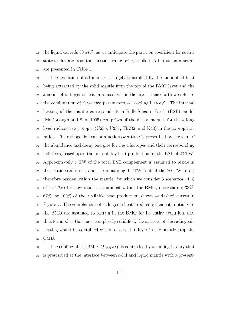
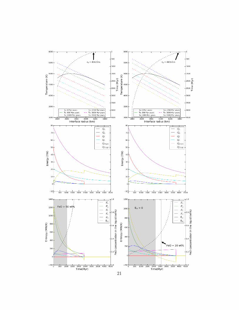
αBMO 0.3 0.3 0.4 0.4 0.4 0.4 0.3 0.3 0.3 0.3 0.4 0.4 0.4 0.4 0.3 0.3

T 0m 700 1100 700 1100 700 1100 700 1100 700 1100 700 1100 700 1100 700 1100

Cooling history model: H QpresentBMO = 15 TW, Qr = 4 TW, Qpresent

CMB = 11 TW

EΦ 280 215 351 21 1 -30 -9 -35 265 182 324 222 -40 -80 -50 -83

tX (Myr) 1050 1390 1070 1430 1690 2550 1670 2520 1540 1860 1600 1920 2600 3590 2560 3540

tΦ (Myr) 2200 2810 2370 3080 1690 2210∗ 1620∗ 2120∗ 2920 3160 3240 3470 2250∗ 2560∗ 2140∗ 2450∗

tBMO (Myr) 2420 4070 2480 4180 2330 3930 2310 3890 4020 4180 3820 3750

TfinalCMB (K) 4258 4310 4279 4334 4228 4279 4220 4270 4500 4433 4533 4458 4453 4401 4438 4390

Cooling history model: n QpresentBMO = 18 TW, Qr = 4 TW, Qpresent

CMB = 14 TW

EΦ 453 360 566 434 49 15 34 6 484 364 584 435 18 -24 7 -32

tX (Myr) 750 960 760 980 1160 1620 1150 1610 1060 1250 1100 1280 1690 2170 1660 2150

tΦ (Myr) 1560 2100 1610 2250 1300 1700 1250 1640 2200 2500 2390 2700 1760 2050∗ 1690 1980∗

tBMO (Myr) 1590 2370 1630 2420 1540 2310 1530 2290 2430 3350 2510 3440 2330 3230 2300 3190

TfinalCMB (K) 3668 3684 3690 3705 3638 3654 3630 3645 3908 3864 3943 3894 3862 3823 3848 3811

Cooling history model: u QpresentBMO = 18 TW, Qr = 8 TW, Qpresent

CMB = 10 TW

EΦ 284 217 347 263 1 -31 -7 -35 267 183 322 220 -43 -81 -48 -84

tX (Myr) 1090 1460 1120 1490 1770 2730 1750 2700 1610 1960 1670 2020 2780 3920 2730 3850

tΦ (Myr) 2290 2940 2470 3220 1780 2360∗ 1710∗ 2270∗ 3050 3330 3370 3640 2400∗ 2740∗ 2290∗ 2630∗

tBMO (Myr) 2570 4490 2640 2480 4320 2450 4270 4410 4170 4100

TfinalCMB (K) 4342 4399 4363 4418 4312 4366 4303 4357 4583 4502 4613 4525 4536 4471 4522 4460

Cooling history model: l QpresentBMO = 21 TW, Qr = 8 TW, Qpresent

CMB = 13 TW

EΦ 488 390 592 464 60 25 45 15 517 398 623 470 30 -14 19 -22

tX (Myr) 740 950 760 970 1150 1610 1140 1600 1060 1240 1090 1270 1680 2160 1650 2140

tΦ (Myr) 1550 2100 1600 2240 1310 1720 1270 1670 2220 2530 2390 2730 1780 2090∗ 1720 2030∗

tBMO (Myr) 1580 2360 1620 2410 1540 2300 1520 2280 2420 3340 2500 3430 2320 3220 2290 3180

TfinalCMB (K) 3671 3686 3693 3707 3642 3657 3633 3648 3911 3866 3946 3896 3865 3825 3851 3812

Cooling history model: s QpresentBMO = 21 TW, Qr = 12 TW, Qpresent

CMB = 9 TW

EΦ 303 234 365 275 5 -28 -2 -32 280 196 332 230 -39 -79 -45 -81

tX (Myr) 1100 1480 1130 1520 1810 2820 1790 2790 1650 2010 1710 2070 2870 4090 2820 4020

tΦ (Myr) 2340 3040 2530 3310 1850 2480∗ 1780∗ 2400∗ 3150 3470 3470 3780 2510∗ 2900∗ 2410∗ 2800∗

tBMO (Myr) 2640 2720 2550 2520 4480 4360 4290

TfinalCMB (K) 4379 4432 4401 4452 4350 4404 4342 4396 4617 4533 4644 4556 4575 4503 4561 4492

∗ represents the last instance in time when EΦ > 0.

12

day value of 15, 18, and 21 TW shown as solid curves in Figure 2. Thus,191

the core heat flow across the CMB, Qcmb, at the present day spans values192

between 9-14 TW, which is the difference between QBMO and Qr for the193

cooling histories considered in Table 1. The differences between QBMO and194

Qr for the various combinations also imply higher or lower secular cooling195

rates for the mantle, as the larger value chosen for Qr leaves a smaller amount196

of the available 12 TW for heating the mantle above the BMO. For example,197

Qr of 8 TW in the BMO leaves only 4 TW in the solid mantle, leading198

to faster secular cooling of the mantle which would presumably drive faster199

secular cooling of the core, and hence this value of Qr is used in combination200

with larger QBMO values of 18 TW and 21 TW, corresponding to Qcmb values201

of 10 and 13 TW, respectively.202

2.3. Entropy budget203

As mentioned above, the energy budget alone provides enough informa-204

tion to determine the thermal evolution of the BMO layer. However, in205

order to fully characterize its magnetic evolution and, ultimately, determine206

the feasibility of dynamo activity, the entropy balance equations are required.207

Most importantly, the entropy associated with thermal conduction down an208

adiabat, Eκ, and the Ohmic heating play crucial roles in determining if a209

dynamo is energetically favorable once all sources of entropy are considered.210

An equation analogous to 1 can be written for the entropy budget identifying211

both sources and sinks, and cases for the core have been extensively derived212

elsewhere (Gubbins et al., 2003, 2004; Nimmo, 2015). Below, we only present213

their final formulations and describe any changes made in adapting them to214

13

Figure 2: Cooling histories. The three different cooling histories imposed for all model runs (#1-16 in

Table 2) representing 15, 18, and 21 TW present-day, adiabatic heat flux across the top of the BMO layer

are shown as solid lines. Dashed lines show the three different radiogenic heating curves 4, 8, and 12 TW

resulting from assuming that roughly 30%, 70%, and 100% of the BSE radioactive element budget are

initially sequestered within the BMO layer.

14

describe our model. The entropy budget is as follows215

Es + Eg + Er + EL + EP + EH = Ek + EΦ, (9)

where Es, Eg, Er, EL, EP , and EH are the sources and Ek, EΦ are the sinks;216

k is the thermal conductivity of the layer, and Φ represents the combined217

viscous and Ohmic dissipation, though the former is assumed to be negligible218

(Nimmo, 2015). The small contributions from EP and EH are also ignored in219

this work. Excluding these terms, the analytical expression for the entropy220

budget is as the following221

−∫ρCp

(1

Tc− 1

T

)dTBMO

r

dtdV +

Qg

T+

∫ρh

(1

Tc− 1

T

)dV

− 4πr2iLH(Ti − Tc)

(dTm/dP − dT/dP )T 2c g

dTBMOr

dt=

∫k

(∇TT

)2

dV +

∫Φ

TdV,

which is comparable to 8 except for the Carnot efficiency term, (1/Tc−1/T ).222

The criteria of EΦ > 0 is commonly used for determining whether the223

model can generate a dynamo subject to the same assumptions that govern224

the applicability of this approach to core dynamics (Gubbins et al., 2004;225

Nimmo, 2015; Buffett et al., 1996; Labrosse, 2003), that the fluid is elec-226

trically conductive, rapidly rotating, and undergoing vigorous convection to227

remain adiabatic and homogenous, all of which are also appropriate for the228

scenario of a basal magma ocean. This framework is easily adaptable to229

determining the Ohmic dissipation within a BMO layer. The expression for230

the first three terms remain the same but the integration bounds must be231

adapted to encompass the evolving thickness of the BMO layer. However,232

the term for entropy production due to the release of latent heat at the in-233

terface, EL, which depends on the cooling rate of the layer and the difference234

15

between the slopes of the adiabat and the melting curve, is different to the235

analogous core case.236

For the case of the inner core growing outward, the adiabat and the melt-237

ing curve are anchored at two distinct temperatures; the CMB temperature238

for the adiabat and the interface (inner-core boundary (ICB)) temperature239

for the liquidus. However, for the BMO layer crystallizing downward to-240

wards the CMB, both the adiabat and melting curve are anchored at the241

same point. This results in (Ti − Tc) in EL to be zero. Another way to242

think about this is to consider where the latent heat is being generated. In243

the case of the core, latent heat is released at the ICB which drives convec-244

tive motions throughout the liquid outer core directly above; but for a BMO245

layer, the latent heat is generated at the top of the liquid layer, so it does246

not contribute to convection in the liquid below. Finally, it is clear from247

these equations that aside from requiring entropy sources to be sufficiently248

energetic to power the dynamo, Ek cannot be too large (i.e. large values of249

k) as this would result in most of the entropy being conducted away along250

the adiabat and not be available to power a dynamo.251

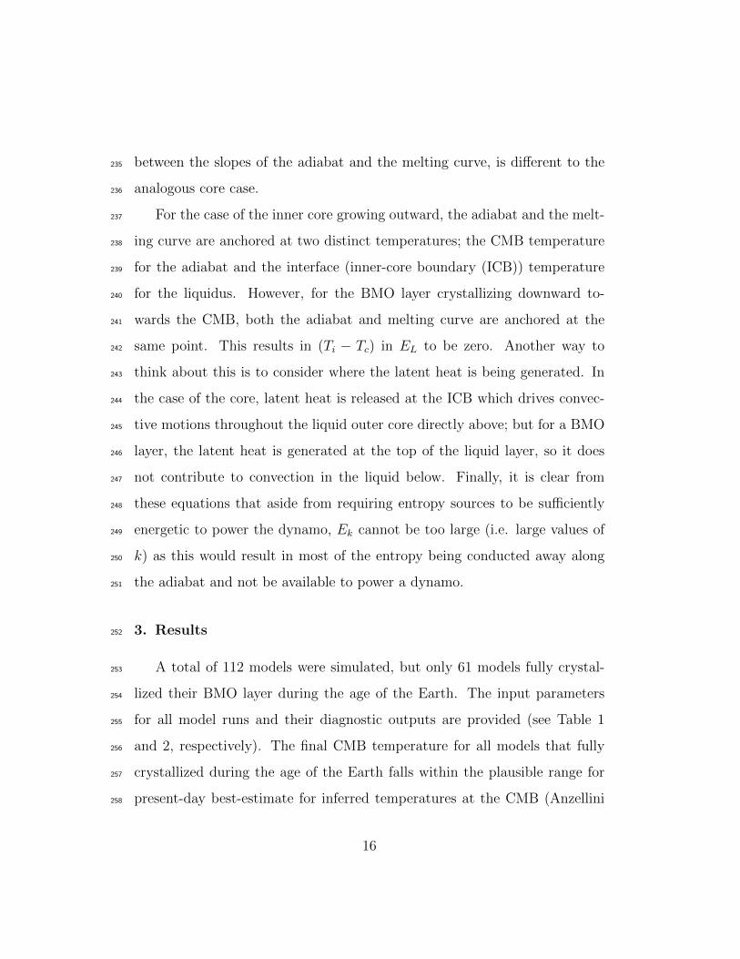
3. Results252

A total of 112 models were simulated, but only 61 models fully crystal-253

lized their BMO layer during the age of the Earth. The input parameters254

for all model runs and their diagnostic outputs are provided (see Table 1255

and 2, respectively). The final CMB temperature for all models that fully256

crystallized during the age of the Earth falls within the plausible range for257

present-day best-estimate for inferred temperatures at the CMB (Anzellini258

16

et al., 2013) as shown in Figure 3.259

The longevity of the BMO layer varies greatly between models, ranging260

from short-lived layers crystallizing in 1.5 Gyrs to long-lived layers taking as261

much as 4.5 Gyrs to fully crystallize. The dominant parameters controlling262

the thermal evolution of the BMO layer are the imposed depression on the263

melting curve and the adiabatic gradient; these effects are shown schemat-264

ically by arrows in Figure 3. For a given cooling history, imposing a larger265

melting-point depression extends the life of the BMO layer but it has a neg-266

ligible effect on the final CMB temperature. However, introducing a steeper267

adiabatic gradient (dTa/dr = 1 K/km for filled marker vs dTa/dr = 1.2268

K/km for unfilled markers in Figure 3) not only extends the time it takes269

the BMO layer to fully crystallize, but it also results in a hotter present-day270

CMB temperature. Changing both parameters simultaneously appears to271

have an almost linear additive effect.272

The general trend observed in Figure 3 is primarily controlled by the273

total heat budget available to drive the BMO evolution, as defined by the274

particular cooling history imposed (i.e. combination of QpresentBMO and Qr from275

Figure 2). Indeed, the fastest cooling models, those on the bottom left,276

have a bigger heat budget than the slower cooling models on the top right.277

Moreover, our choice of curves forQBMO andQr and their inherent curvatures278

causes the effects due to melting-point depression and adiabatic gradient to279

be more pronounced on the slower cooling models, with some of these taking280

as much as 4.5 Gyrs to fully crystallize. A batch of 32 models with QBMO281

= 12 TW and Qr = 4 and 8 TW (corresponding to QCMB = 8 and 4 TW,282

respectively) were probed and none successfully crystallized the entirety of283

17

their BMO layer during the 4.5 Gyrs time window. Indeed, 19 other models284

with the cooling histories reported here were also unsuccessful (see Table 2).285

Given the large group of successful models, we focus on two models which286

best represent the extensive range of evolution scenarios generated by our287

choices of parameters. Moreover, these reference models resemble the model288

proposed by (Ziegler and Stegman, 2013). The complete temperature, energy,289

and entropy evolution for models #1 and #15 are respectively shown in the290

top, middle, and bottom panels of Figure 4.291

The evolution of the temperature and the interface radius between the292

liquid, crystallizing BMO layer and the solid mantle above for each model293

is shown in Figure 4A and B. Both models share the same imposed cooling294

history with QBMO = 15 TW and Qr = 4 TW, but have two different dTa/dr295

values. The initial thickness of the BMO (i.e. interface radius) is defined by296

the intersection of the melting curve (solid black line) with the adiabat (see297

Figure 1), and its evolution is controlled by the cooling rate of the layer298

which is directly dominated by the amount of heat being extracted from the299

layer, as prescribed by the cooling history curve. As the layer cools over300

time, the adiabat evolves to lower temperatures (shown as colored dashed301

lines) intersecting the melting curve at greater depths causing the interface302

radius to decrease and the liquid layer to shrink towards the CMB. Indeed,303

the retarding effect dTa/dr has on the evolution of the layer (shown in Figure304

3) is evident here as model #1 crystallizes about 1 Gyr sooner than model305

#15 with the steeper adiabatic gradient.306

All the terms in the energy budget outlined in Eq. 8 for both models307

including an imposed core cooling (yellow curve) term are shown in Figure308

18

Figure 3: Final CMB temperature. The present-day CMB temperature for all models that successfully

crystallized during the age of the Earth are plotted at their corresponding crystallization time. Both

adiabatic gradients, dTa/dr = 1 (filled markers) and dTa/dr = 1.2 (unfilled markers) and both melting

point depressions to the melting curve, 700 K (red) and 1100 K (blue) are shown. Schematic arrows show

the effect of either parameter in the longevity of the BMO layer for any model run (depicted by the model

run numbers) within a given model setup (markers in legend).

19

4C and D. The most energetic source during the evolution of the BMO layer309

is the latent heat released as the layer crystallizes, while gravitational rear-310

rangement and secular cooling terms are small. The amount of latent heat311

released is the largest during the first billion years of evolution as this is when312

the crystallization rate is the fastest before being retarded by the imposed313

melting-point depression on the melting curve. When the layer crystallizes314

to a thickness of ≈200 - 300 km, the latent heat term becomes comparable315

to the radiogenic heating and the crystallization rate decreases significantly.316

Once the layer reaches the CMB, the radiogenic elements are assumed to317

be trapped in a thin layer atop the CMB, while QL and Qg terms become318

zero which results in a corresponding jump in core heat flow. The remaining319

thermal evolution is primarily accommodated by secular cooling of the core320

according to the prescribed thermal history model (QBMO) and the assumed321

heat capacity of the core, resulting in the final TCMB values shown in Figure322

3.323

20

21

Figure 4: BMO layer evolution. Representative models with QBMO = 15 TW and Qr = 4 TW showing

the temperature, energy, and entropy evolution of a 762-km and 978-km thick BMO layer for Models #1

(left column) and Model #15 (right columb), respectively. The evolution of the temperature and thickness

of the BMO layer over time controlled by the different adiabatic gradients (dTa/dr = 1 K/km for Model

#1 and dTa/dr = 1.2 K/km for Model #15) are shown on panel A and B, respectively. Each term in the

energy budget outlined in Eq. 1 is plotted in C and D for both models over time. The evolution of the

associated entropy terms (solid curves) and evolution of the FeO concentration (dashed curve) over time

are shown in E and F. Shaded regions show the time interval where EΦ > 0 while the FeO concentration

in the liquid is below 50 wt% (panel E), and last instance when EΦ > 0 in panel F (i.e. when FeO

concentration in run #15 reaches 50%, EΦ < 0).324

The terms in the entropy budget outlined in Eq. 9 for each model are325

shown in Figure 4E and F, along with the corresponding evolution of the326

FeO concentration in the liquid layer. As described in the Methods section,327

the latent heat term is zero for the scenario being considered here. While the328

gravitational term is small in the energy budget, it is the main contributor329

of entropy to the system (green curve), with the secular (blue curve) and330

radiogenic (light blue curve) terms contributing marginally. The cumulative331

total of these entropy sources is balanced against both thermal conduction332

(magenta curve) and Ohmic dissipation (yellow curve), which are the entropy333

sinks in the system.334

The entropy of thermal conduction is approximately constant and scales335

with the choice of thermal conductivity, which is 8 W/m/K for these models.336

Both models sustain EΦ > 0 for the first ≈2 billions years, indicating a337

dynamo would be present in both models over that period of time. However,338

for BMO dynamos, we consider an additional criteria of whether DFeO is339

still consistent with the system once it has become highly enriched in Fe.340

Consequently, we adopt a value of clFeO = 50wt% for this threshold, which341

22

is shown in the shaded regions. Model #15 (Figure 4F) falls below EΦ = 0342

before this threshold is reached, and for such models as this, we report their343

dynamo cessation time (starting from tΦ=0) as the last instance when EΦ >344

0. In contrast, Model #1 (Figure 4E) reaches the threshold while EΦ is still345

positive, and for models that encounter this situation, we report the time346

they reach this threshold as their dynamo cessation.347

We consider this threshold value as a conservative estimate given that348

EΦ is well above zero when this point is reached and it would be likely for349

a dynamo to be operating beyond this time. The partitioning of Fe into the350

remaining liquid at the solidification front is the mechanism for generating351

gravitational entropy, which is the dominant term in the entropy budget and352

controls the magnitude of the Ohmic dissipation. The rate at which the353

fluid is enriched with Fe, and speed at which the threshold value is reached,354

is determined by the value of DFeO. Model #1, with DFeO = 0.1, results355

in clFeO increasing more rapidly (dashed line in Figure 4E) than measured356

increases of clFeO in Model #15, with DFeO = 0.5 (dashed line in Figure 4F).357

Therefore, the dynamo generated by model #1 (Figure 4E) is roughly 20%358

more energetic than that of model #15 (Figure 4F).359

The amount of entropy available to sustain a dynamo varies among all360

successful models. Model results for all runs including the available entropy361

(at clFeO = 50wt%), their corresponding dynamo and BMO cessation times,362

and their final CMB temperatures are shown in Table 2. Figure 5 shows the363

amount of Ohmic dissipation at the time the BMO composition encountered364

the threshold value of clFeO = 50wt% for all models that fully crystallized365

within the age of the Earth. The two clear populations of models shown366

23

in Figure 5 are primarily controlled by the two, end-member values for the367

partition coefficient of FeO. Models with DFeO = 0.1 (Nomura et al., 2011)368

give rise to long-lived dynamos with lower Ohmic dissipation while those369

with DFeO = 0.5 (Andrault et al., 2012) result in dynamos that are short-370

lived and larger values of EΦ. Both scenarios, however, result in models with371

sufficiently large EΦ values for the first 1.5 Gyrs -implying an active dynamo372

during this time.373

Combining our results from Figure 3 for how long it takes the BMO layer374

to fully crystallize and, in each of those models, how long a dynamo would375

be active from Figure 5, we can see there exists a wide range of scenarios for376

a BMO dynamo as shown in Figure 6. These scenarios can be summarized377

in four distinct populations: Short-lived BMO with (1) short-lived, intense378

dynamo, and (2) long-lived, weaker dynamo; and long-lived BMO with (3)379

short-lived, intense dynamo, and (4) long-lived, weaker dynamo.380

The intensity of the dynamo is regulated by the value of DFeO while381

the time required for the layer to completely solidify is controlled by both382

melting-point depression and the choice of adiabatic gradient. Those models383

with the smaller melting-point depression (e.g. T 0m = 700 K) and a partition384

coefficient DFeO = 0.1 result in short-lived BMO layers with roughly 60%385

more entropy available (at clFeO = 50wt%) to sustain a dynamo compared386

to the cases with DFeO = 0.5. A smaller DFeO value results in faster Fe387

enrichment of the liquid layer and correspondingly higher values of entropy388

generated due to the larger density jump at the interface (e.g. larger Eg389

term). Indeed, extending the timescale for solidification of the BMO, by390

imposing a larger melting-point depression, increases the amount of entropy391

24

Figure 5: Entropy of Ohmic dissipation over time for all models (at clFeO = 50wt%) whose BMO layer

fully crystallized during the age of the Earth plotted in black (filled). For models with EΦ < 0 at this

cutoff, their entropy value is plotted at the last time when it was positive in black (unfilled). Markers

indicate the five difference QBMO-Qr scenarios imposed as described in the text. Two distinct clusters,

indicated by the shaded regions, capture the influence of the two different partition coefficient values.

25

available to sustain magnetic activity for a longer period of time. It is plau-392

sible to have models extending the entire shaded area in Figure 6 through a393

different combination of allowable model parameters and a less conservative394

cutoff (i.e. > clFeO = 50wt%).395

4. Discussion396

The present-day CMB temperature for all successful models shown here397

(Figure 3) falls within a plausible value (4000±500 K) for the best estimates398

up to date (Anzellini et al., 2013). The thermal evolution of a BMO layer399

atop the liquid core over time is heavily dominated by two parameters: the400

adiabatic gradient in the liquid, and the melting curve for a lower mantle401

composition; most importantly how depressed this curve becomes at near-402

CMB pressures and temperatures.403

The entropy budget of a BMO-powered dynamo are heavily dominated404

by the choice in partition coefficient for FeO in the liquid, and, in particular,405

its evolution as the layer becomes heavily-enriched; such behavior is poorly406

constrained up to date. We anticipate that DFeO will actually start closer to407

a value of 0.1 (Nomura et al., 2011) and evolve to larger values as the BMO408

layer decreases in size, thus we believe our end-member choices for DFeO409

bracket the expected behavior. Such evolution would in turn result in highly410

energetic dynamo for the first few hundred million years, similar to Figure411

4E, with sustained Ohmic dissipation values beyond 2 Gyrs, resembling the412

scenario shown in Figure 4F with the higher DFeO value.413

Our models successfully show that a crystallizing BMO can be an effec-414

tive mechanism for generating and sustaining a dynamo throughout early415

26

Figure 6: Duration of dynamo activity versus BMO layer crystallization time for all models that fully

crystallized. Models with EΦ > 0 at clFeO = 50wt% are plotted in black (filled), while those whose EΦ

value was negative at clFeO = 50wt% are plotted in black (unfilled) at the last time EΦ was above zero.

Shaded regions as per Figure 5.

27

Earth. Most importantly, all models whose BMO layer successfully crystal-416

lized during the age of the Earth have sufficient entropy to generate magnetic417

activity for at least the first 1.5 Gyrs (Figure 5), with some lasting well passed418

2 Gyrs. A vast range of parameter combinations other than the choices we419

made would also lead to scenarios with enough entropy to generate a dynamo420

for at least 1.5 Gyrs, conservatively. This makes a BMO-driven dynamo a421

plausible mechanism for explaining the existence of a magnetic field early422

on in Earth’s history as required by paleomagnetic observations; thus relax-423

ing the need for a global magnetic field to be entirely powered by thermal424

cooling of the core. Additionally, since exsolution-based mechanisms are also425

contingent upon the presence of a BMO of some depth, the BMO-powered426

dynamo is not mutually exclusive with them and the possibility exists for427

both to operate, either contemporaneously or sequentially.428

The time required to fully crystallize a BMO layer as well as the dura-429

tion of a dynamo that such evolution would produce varies greatly among430

models (Figure 6). However, it is possible to have some scenarios where a431

dynamo can be sustained (e.g. EΦ > 0) for a longer time window given the432

conservative cutoff employed here, all while also constraining its BMO layer433

to be fully crystallized at present day and a CMB temperature in agree-434

ment with current best estimates. Previous work emphasized that ”thermal435

catastrophe” outcomes were constraints for model evolutions and used this436

as a basis for determining which combinations of parameters were deemed437

successful (Korenaga, 2013, 2008; Driscoll and Bercovici, 2014), however, by438

these standards all of our models would be unsuccessful which demonstrates439

this logic is not sound. Instead, we propose the only constraint that must440

28

be satisfied is that the mantle with an initial BMO must completely solidify441

within the age of the Earth, and if not, this is what we would refer to as un-442

successful model. There is nothing catastrophic or implausible about thermal443

evolutions that exceed the solidus temperatures for part of their evolution.444

5. Conclusion445

The evolution of a crystallizing basal magma ocean overlying the liquid446

core can explain the magnetic evolution of early Earth as most models tested447

here are energetic enough to sustain a dynamo during this time. Indeed, some448

of the models sustain dynamos well into the Archaen, though marginally.449

The evolution of a basal magma ocean, as modeled here, depends heavily450

on the material properties of silicates in general and silicate melts in par-451

ticular. Parameters such as the partitioning coefficient for a molten silicate452

layer and its evolution as the layer becomes highly enriched in FeO (i.e.453

clFeO > 50 wt%), as well as the associated melting-point depression of such454

a composition at near-CMB pressure and temperature conditions are crucial455

parameters yet they are poorly constrained to date. The work presented456

here, while it provides a novel mechanism to generate a dynamo and under-457

stand Earth’s complex magnetic history, should serve as motivation to better458

constrain these parameters experimentally.459

Moreover, the versatility of this model does not hinge on a specific con-460

dition of core cooling; in fact, it can be adapted to complement thermal evo-461

lution models involving any thermal conductivity values for the core. More462

importantly, this model complements previous dynamo mechanism proposed463

by being able to generate enough power to induce and sustain an early dy-464

29

namo whose lifespan can be extended by different mechanism (e.g. the Mg465

exsolution of (O’Rourke et al., 2017)). A similar computational formula-466

tion can be relevant to simulate thermal history schemes in ”super-Earth”467

exoplanets.468

Acknowledgements469

We acknowledge C. Davies for providing the idea of calculating the en-470

tropy budget for the BMO and for providing the code used for (Davies, 2015)471

for us to adapt. We thank J. Badro, C. Boukare, L. Stixrude, S. Stewart for472

helpful discussions. We acknowledge support from NSF.473

References474

Andrault, D., Petitgirard, S., Nigro, G. L., Devidal, J.-L., Veronesi, G.,475

Garbarino, G., Mezouar, M., 2012. Solid–liquid iron partitioning in Earths476

deep mantle. Nature 487 (7407), 354.477

Anzellini, S., Dewaele, A., Mezouar, M., Loubeyre, P., Morard, G., 2013.478

Melting of iron at Earths inner core boundary based on fast X-ray diffrac-479

tion. Science 340 (6131), 464–466.480

Badro, J., Aubert, J., Hirose, K., Nomura, R., Blanchard, I., Borensztajn,481

S., Siebert, J., 2018. Magnesium Partitioning Between Earth’s Mantle and482

Core and its Potential to Drive an Early Exsolution Geodynamo. Geophys-483

ical Research Letters 45 (24), 13–240.484

Badro, J., Siebert, J., Nimmo, F., 2016. An early geodynamo driven by485

30

exsolution of mantle components from Earths core. Nature 536 (7616),486

326.487

Boukare, C.-E., Ricard, Y., 2017. Modeling phase separation and phase488

change for magma ocean solidification dynamics. Geochemistry, Geo-489

physics, Geosystems 18 (9), 3385–3404.490

Boukare, C.-E., Ricard, Y., Fiquet, G., 2015. Thermodynamics of the MgO-491

FeO-SiO2 system up to 140 GPa: Application to the crystallization of492

Earth’s magma ocean. Journal of Geophysical Research: Solid Earth493

120 (9), 6085–6101.494

Buffett, B. A., Huppert, H. E., Lister, J. R., Woods, A. W., 1996. On the495

thermal evolution of the Earth’s core. Journal of Geophysical Research:496

Solid Earth 101 (B4), 7989–8006.497

Canup, R. M., Asphaug, E., 2001. Origin of the Moon in a giant impact near498

the end of the Earth’s formation. Nature 412 (6848), 708.499

Caracas, R., Hirose, K., Nomura, R., Ballmer, M. D., 2019. Melt–crystal500

density crossover in a deep magma ocean. Earth and Planetary Science501

Letters 516, 202–211.502

Cuk, M., Stewart, S. T., 2012. Making the Moon from a fast-spinning Earth:503

a giant impact followed by resonant despinning. Science 338 (6110), 1047–504

1052.505

Davies, C. J., 2015. Cooling history of Earths core with high thermal con-506

ductivity. Physics of the Earth and Planetary Interiors 247, 65–79.507

31

de Koker, N., Steinle-Neumann, G., Vlcek, V., 2012. Electrical resistivity and508

thermal conductivity of liquid Fe alloys at high P and T, and heat flux in509

Earths core. Proceedings of the National Academy of Sciences 109 (11),510

4070–4073.511

De Koker, N., Stixrude, L., 2009. Self-consistent thermodynamic description512

of silicate liquids, with application to shock melting of MgO periclase and513

MgSiO3 perovskite. Geophysical Journal International 178 (1), 162–179.514

Driscoll, P., Bercovici, D., 2014. On the thermal and magnetic histories of515

Earth and Venus: Influences of melting, radioactivity, and conductivity.516

Physics of the Earth and Planetary Interiors 236, 36–51.517

Du, Z., Boujibar, A., Driscoll, P., Fei, Y., 2019. Experimental constrains on518

an MgO exsolution-driven geodynamo. Geophysical Research Letters.519

Du, Z., Jackson, C., Bennett, N., Driscoll, P., Deng, J., Lee, K. K., Green-520

berg, E., Prakapenka, V. B., Fei, Y., 2017. Insufficient energy from521

MgO exsolution to power early geodynamo. Geophysical Research Letters522

44 (22), 11–376.523

Dziewonski, A. M., Anderson, D. L., 1981. Preliminary reference Earth524

model. Physics of the earth and planetary interiors 25 (4), 297–356.525

Fiquet, G., Auzende, A., Siebert, J., Corgne, A., Bureau, H., Ozawa, H.,526

Garbarino, G., 2010. Melting of peridotite to 140 gigapascals. Science527

329 (5998), 1516–1518.528

Gomi, H., Ohta, K., Hirose, K., Labrosse, S., Caracas, R., Verstraete, M. J.,529

Hernlund, J. W., 2013. The high conductivity of iron and thermal evolution530

32

of the Earths core. Physics of the Earth and Planetary Interiors 224, 88–531

103.532

Gubbins, D., Alfe, D., Masters, G., Price, G. D., Gillan, M., 2003. Can533

the Earths dynamo run on heat alone? Geophysical Journal International534

155 (2), 609–622.535

Gubbins, D., Alfe, D., Masters, G., Price, G. D., Gillan, M., 2004. Gross536

thermodynamics of two-component core convection. Geophysical Journal537

International 157 (3), 1407–1414.538

Hirose, K., Morard, G., Sinmyo, R., Umemoto, K., Hernlund, J., Helffrich,539

G., Labrosse, S., 2017. Crystallization of silicon dioxide and compositional540

evolution of the Earths core. Nature 543 (7643), 99.541

Holmstrom, E., Stixrude, L., Scipioni, R., Foster, A., 2018. Electronic con-542

ductivity of solid and liquid (Mg, Fe) O computed from first principles.543

Earth and Planetary Science Letters 490, 11–19.544

Korenaga, J., 2008. Urey ratio and the structure and evolution of Earth’s545

mantle. Reviews of Geophysics 46 (2).546

Korenaga, J., 2013. Initiation and evolution of plate tectonics on Earth:547

theories and observations. Annual review of earth and planetary sciences548

41, 117–151.549

Labrosse, S., 2003. Thermal and magnetic evolution of the Earths core.550

Physics of the Earth and Planetary Interiors 140 (1-3), 127–143.551

33

Labrosse, S., 2015. Thermal evolution of the core with a high thermal con-552

ductivity. Physics of the Earth and Planetary Interiors 247, 36–55.553

Labrosse, S., Hernlund, J., Coltice, N., 2007. A crystallizing dense magma554

ocean at the base of the Earths mantle. Nature 450 (7171), 866.555

Laneuville, M., Hernlund, J., Labrosse, S., Guttenberg, N., 2018. Crystal-556

lization of a compositionally stratified basal magma ocean. Physics of the557

Earth and Planetary Interiors 276, 86–92.558

Lock, S. J., Stewart, S. T., Petaev, M. I., Leinhardt, Z., Mace, M. T., Ja-559

cobsen, S. B., Cuk, M., 2018. The origin of the Moon within a terrestrial560

synestia. Journal of Geophysical Research: Planets 123 (4), 910–951.561

McDonough, W. F., Sun, S.-S., 1995. The composition of the Earth. Chemical562

Geology 120 (3-4), 223–253.563

McWilliams, R. S., Spaulding, D. K., Eggert, J. H., Celliers, P. M., Hicks,564

D. G., Smith, R. F., Collins, G. W., Jeanloz, R., 2012. Phase transforma-565

tions and metallization of magnesium oxide at high pressure and temper-566

ature. Science 338 (6112), 1330–1333.567

Nimmo, F., 2015. Energetics of the core: Ed. G. Schubert. Treatise on geo-568

physics (second edition). Elsevier, Oxford 8, 27–55.569

Nomura, R., Ozawa, H., Tateno, S., Hirose, K., Hernlund, J., Muto, S., Ishii,570

H., Hiraoka, N., 2011. Spin crossover and iron-rich silicate melt in the571

Earths deep mantle. Nature 473 (7346), 199.572

Olson, P., 2013. The new core paradox. Science 342 (6157), 431–432.573

34

O’Rourke, J. G., Korenaga, J., Stevenson, D. J., 2017. Thermal evolution574

of Earth with magnesium precipitation in the core. Earth and Planetary575

Science Letters 458, 263–272.576

ORourke, J. G., Stevenson, D. J., 2016. Powering Earths dynamo with mag-577

nesium precipitation from the core. Nature 529 (7586), 387.578

Pozzo, M., Davies, C., Gubbins, D., Alfe, D., 2012. Thermal and electrical579

conductivity of iron at Earths core conditions. Nature 485 (7398), 355.580

Scipioni, R., Stixrude, L., Desjarlais, M. P., 2017. Electrical conductivity of581

SiO2 at extreme conditions and planetary dynamos. Proceedings of the582

National Academy of Sciences 114 (34), 9009–9013.583

Soubiran, F., Militzer, B., 2018. Electrical conductivity and magnetic dy-584

namos in magma oceans of Super-Earths. Nature communications 9 (1),585

3883.586

Spaulding, D., McWilliams, R., Jeanloz, R., Eggert, J., Celliers, P., Hicks,587

D., Collins, G., Smith, R., 2012. Evidence for a phase transition in silicate588

melt at extreme pressure and temperature conditions. Physical Review589

Letters 108 (6), 065701.590

Stackhouse, S., Stixrude, L., Karki, B. B., 2010. Thermal conductivity of per-591

iclase (MgO) from first principles. Physical review letters 104 (20), 208501.592

Stevenson, D. J., 2003. Planetary magnetic fields. Earth and planetary sci-593

ence letters 208 (1-2), 1–11.594

35

Stixrude, L., 2014. Melting in super-earths. Philosophical Transactions of595

the Royal Society A: Mathematical, Physical and Engineering Sciences596

372 (2014), 20130076.597

Stixrude, L., de Koker, N., Sun, N., Mookherjee, M., Karki, B. B., 2009.598

Thermodynamics of silicate liquids in the deep Earth. Earth and Planetary599

Science Letters 278 (3-4), 226–232.600

Tarduno, J. A., Cottrell, R. D., Davis, W. J., Nimmo, F., Bono, R. K., 2015.601

A Hadean to Paleoarchean geodynamo recorded by single zircon crystals.602

Science 349 (6247), 521–524.603

Tarduno, J. A., Cottrell, R. D., Watkeys, M. K., Hofmann, A., Doubrovine,604

P. V., Mamajek, E. E., Liu, D., Sibeck, D. G., Neukirch, L. P., Usui, Y.,605

2010. Geodynamo, solar wind, and magnetopause 3.4 to 3.45 billion years606

ago. Science 327 (5970), 1238–1240.607

Wolf, A. S., Bower, D. J., 2018. An equation of state for high pressure-608

temperature liquids (RTpress) with application to MgSiO3 melt. Physics609

of the Earth and Planetary Interiors 278, 59–74.610

Ziegler, L., Stegman, D., 2013. Implications of a long-lived basal magma611

ocean in generating Earth’s ancient magnetic field. Geochemistry, Geo-612

physics, Geosystems 14 (11), 4735–4742.613

36