1

THEORY

of

WEALTH (*)

and

UNEMPLOYMENT

____________________________________________________

(Macroeconomics from microeconomics)

(*)

Generation-destruction-distribution

CARLOS A. BONDONE

2

THEORY of WEALTH and UNEMPLOYMENT

(TWU)

CONTENTS

Abstract

Theoretical introduction

Research problem - Object

Theoretical framework

Theory of subjective value

Theory of economic calculus

Empirical economic calculus

Wealth and economic calculus in TWU and SEE

Justification of the research

Research questions

Methodology of the research

The structure of the text

Acknowledgements

Part I

MICROECONOMICS

Microeconomics

The fundamental economic causality in an individual (Gossen-Crusoe)

Need (demand)

Economic good (supply)

Fundamental Economic Causality (FEC)

The closed box

Conclusions of Fundamental Economic Causality

Behavior of the Fundamental Economic Causality in Robinson

a) Decrease of demand (need) of a stock

b) Decrease of supply of a stock

3

Supply and demand of a stock – Two sides of the same coin

The closed box of the stock and E point of stock generation

Synthesis of point E

Conclusion of microeconomics

Part II

MACROECONOMICS

Macroeconomics

THE QUANTITY - PRICE

Law of exchange –The fundamental economic causality in a society

The law of exchange and uncertainty

The Quantity-Price and point E of exchange

Quantities-Prices as a unit of measure

The closed box of exchange explains the variation of quantities – prices

Quantity-price and Pareto’s Optimal

The benefit of demand

a) Geometrical expression of the benefit of demand

b) Arithmetical expression of the benefit of demand

Quantity-price, value, and the benefit of demand

Quantity-price theory

CURRENCY

The economic good currency in exchange

The quantity-price of the economic good currency

Variation of the quantity-price of the economic good currency

Quantities-prices relative to the quantity-price of the economic good currency, as a unit of

calculus

ECONOMIC CALCULUS

WEALTH – Calculus and distribution

Stock and calculus of wealth

Robinson’s stock of wealth

Stock of aggregate wealth of “n” owners

Property of the stock of aggregate wealth of “n” owners

Curve of stock and distribution of wealth of “n” owners

4

Conclusion

WEALTH – Generation and destruction

Curve of Generation of Wealth (by “n” owners)

Displacements of the Curve of Wealth Generation (by “n” owners)

Curve of Wealth Destruction (by “n” owners)

Displacements of the Curve of Wealth Destruction (by “n” owners)

ECONOMIC EVOLUTION OF OWNERS

POINT R of average velocity of net positive wealth generated, per capita of owners

Theoretical connotation of point R – Generation of wealth and economic calculus theorems

Behavior of the R point

Curve of the Economic Evolution of Owners (CEE-O)

Displacement of CEE-O from a spatio-temporal point

SOCIO-ECONOMIC EVOLUTION ― Endogenous institutions and economic policies

Part III

PROPOSED MACROECONOMIC MODEL ― APPLIED

Currency and fiscal policy

Socio-economic evolution in history

Quantities-Prices control, subsidies, and other policies

Appendix A – Charts 36 amplified

Appendix B – Epistemology

Concept of evolution

Continuity for explaining the discrete

Conclusion

Appendix C – Accounting practice for economic calculus without a currency veil

Notes

Charts

Tables

Bibliography

5

Epistemology

Economics

Accounting

6

ABSTRACT

The Theory of Wealth and Unemployment (TWU) postulates that generation, destruction, and

distribution of wealth, and unemployment derive from combining the laws that govern homo

economicus and homo sociologicus. Which implies understanding the laws and variables that

govern the market and the laws and variables that govern (economic) policies.

The model of Socio-Economic Evolution (SEE) we present proves the validity of the

postulate of TWU, insofar as it considers both the laws and variables that govern the market, and

the laws and variables that govern (economic) policy as endogenous to it.

7

THEORETICAL INTRODUCTION

“My pencil is smarter than I” (1)

Albert Einstein

Since this introduction presents theoretical, empirical, and epistemological content, this

introduction is part of the theoretical material to be studied, insofar as here you will find the

basics of the Theory of Wealth and Unemployment (TWU) that we present, and of its model of

Socio Economic Evolution (SEE). Denomination that could alternatively be the model of

political-economic evolution, but considering that social is a broader concept, we will retain the

first. What is important is to begin by stating that the model explains the basics of TWU, based

on considering them endogenous to the market and politics. Thus, with the laws that govern both

scenarios, all variables involved are considered simultaneously ―which we summarize in the

concepts of physical marginal productivity and marginal subjective valuation.

RESEARCH PROBLEM - OBJECT

Since we are speaking of a new theoretical proposal, it is pertinent to introduce the

theoretical framework in which it is developed.

THEORETICAL FRAMEWORK

It is pertinent to offer an introductory summary of the theoretical postulates on which the

proposal is based that, though we say it is new, we must not forget to mention that while TWU

can be considered an extension of the Theory of Economic Time (TET) ―economic time and its

price, interest, are expressed in changes in economic value, therefore, understanding the basics

implies understanding those entities― (2)

, and the SEE model operates as a demonstration of its

hypothesis.

This section therefore anticipates the theoretical framework of the proposal, which we will do

highlighting the central primitive terms.

Theory of subjective value

Considering the epistemological answer states that the macro is based on the micro sphere,

we will show how all humans make the individual and “abstract” act of valuing subjectively

“visible”. The hypothesis of this work is that humans manifest their subjective valuation through

quantities of economic goods, be it the case of Robinson Crusoe ―that values without prices―

or that of a plurality of individuals that exchange in a society ―they value with price-quantities

derived from exchange, be it through barter or with currency.

The model shows that the subjective value (the value that humans assign “ordinally” to

economic goods):

8

Is implicit in the marginal laws of decreasing utility and increasing marginal effort

(inverse of the law of decreasing yields) which will allow us to obtain an observational

scientific range for subjective value, both at the time we appreciate the utility obtained by

economic goods, and the effort necessary to obtain them given their scarcity.

It is expressed or it manifests itself observationally through quantities of economic goods.

It is measurable, which implies the feasibility of economic calculus, which leads to the

following section. I.e., considering the fallibility typical of any measurement, humans

measure in quantities of economic goods, which allow economic calculus in economics.

This abstract theoretical relation between subjective value and its “empirical” expression, in

observable quantities of economic goods, would allow us to say that an alternative title to the

SEE model could be Quantitative model of subjective value, a suggestion that is very enriching

for economic theory, which in turn introduces us to economic calculus.

Theory of economic calculus

The act of valuing subjectively is behind all human economic calculus, calculus that guides

economic actions. In turn, the fundamental economic calculus humans carry out is of the effort

needed to obtain economic goods, and the use to which they will be put, all in a limited spatio-

temporal period.

Understanding the way in which humans generate (effort) and dispose of (destruction)

temporarily of economic goods, in a finite spatio-temporal field, is the priority for economics as

a science. This whole work refers to those calculus (effort and satisfaction), including two

spheres of human action: understanding the calculus by Robinson Crusoe (calculus of quantities

―of economic goods― without prices) and the calculus by “First” Robinson and “Second”

Robinson when they exchange economic goods (calculus in quantities ―of economic goods―

with prices; in this case with or without currency).

Thus, we call economic value the human valuation of quantities of economic goods, which

also implies saying that economic calculus works with quantities of economic goods. In turn, we

define as currency value ―a concept we define based on Menger and Mises― the economic

value pondered by currency units. All which has theoretical and empirical transcendence

insofar as it allows us to build a theory and model of an only real and currency world at the

same time, with no need to explain a real world versus a virtual currency world, that must be

balanced. The two world dichotomy initiated by Böhm-Bawerk and Wicksell,(3)

that conditioned

all the developments of the twentieth century ― “Wicksell’s Real Effect” and “Wicksell’s Price

Effect”, and Patinkin’s dichotomies.

Let us see then a very short summary of the aspects we must consider in reference to

economic calculus, that also can be used to show that micro economic calculus (calculus without

prices) underlies macro-economic calculus (calculus with prices, that implies barter and

currency value), since in both, calculus is based on quantities of economic goods:

Temporality of economic calculus: we should not proceed with empirical economic

calculus without stressing that the same refers essentially to how to explain the temporal

9

relation between human beings ―distribution and unemployment―, in a specific spatio-

temporal setting. Temporal relations that include these aspects that need to be calculated:

a) The utility of generating wealth: governed by the temporal law of decreasing

marginal utility.

b) The effort to generate wealth: governed by the temporal law of increasing marginal

effort, in line with the well known law of decreasing marginal yields.

c) The destruction of wealth generated with effort to produce utility: governed by the

temporal law of increasing marginal destruction.

Three calculus governed by their respective laws that, being marginal, allow us to consider

simultaneously the economic preference in time of: the wealth generated and destroyed, its

distribution, and unemployment, all in terms of quantities of economic goods (currency value in

a currency regime).

I.e., human decision is guided temporally by amounts of economic goods, available in

specific spatio-temporal area, which will be destined for destruction in said period ―satisfaction

of needs in the referred period― and for saving for future destruction. Thus, the hypothesis is

that humans demand present goods, both to satisfy present need and as stock for future needs.

Measurability of economic calculus: The model will show that the use of economic value

is not only necessary, but sufficient representation of subjective value, insofar as we will be able

to explain using economic calculus by means of quantities of economic goods ―which will have

been previously categorized in their qualitative aspects, in terms of the need they satisfy.(4)

A

situation that does present a different argument in the “micro” case of Robinson Crusoe, that

calculates quantities of economic goods without prices, since there is no exchange, and the

“macro” case of “First” and “Second” Robinsons, that calculate using prices derived from the

exchange of economic goods among them ―by means of barter or with currency. This is so,

insofar as prices are nothing more than quantities of economic goods. Thus, in this case we do

economic calculus ―we obtain the economic value― by means of the use of quantities of other

economic goods they are exchanged for, which is the essence of the concept of price.

Unit of measure for universal calculus: finally, the specific case of the use of quantities

of an economic good as the universal measure for all calculus ―the currency value― still

belongs to the use of quantity (of economic goods) to ponder and homogenize economic

calculus. In other words, the monetary value homogenizes the economic value, derived from

quantities of economic goods.

Concretely, humans in society calculate by quantities of an economic good used as universal

unit of measure, which allows us to understand human economic action with no “currency veil”.

The fact that the economic unit of measure is not constant in time is solved by humans

considering the error this implies does not prevent them from calculating, which is the reason for

the existence of the universal unit of measure. Which in turn allows humans to see when and

how the dimension of the error prevents calculus ―extreme distortion of currency policies.

10

Empirical economic calculus

Having understood the why (of the decisions humans make in their temporal relation with

economic goods, and the economic relations of humans among themselves), and the how (by the

use of quantities of economic goods), from economic calculus we proceed to explaining the

model proposed as the procedure for human economic calculus. A proposal that explains the use

of quantities without price (Robinson Crusoe), quantities pondered by amounts of other

economic goods with which there is barter, and finally the exchange for quantities of the

economic good chosen as the universal unit of measure, in a society where there is exchange

with currency.

Economic value – calculus without price (Robinson Crusoe that does not exchange)

The use of the laws of decreasing marginal utility (that guides demand) and of increased

efforts (that guides supply) determines the temporal behavior of the satisfaction of needs

provided to Robinson by the economic goods available to him, and the temporal behavior

represented by the effort he will have to make to obtain them, all within the same spatio-

temporal setting. Temporal behavior that will quantify –in specific amounts of economic goods-

the quality of the economic good, and will explain the temporal relation between human needs

and the economic good that satisfies them. Thus, this work will be able to show how what we

call the axiom of the fundamental economic causality, (5)

the ordered set man (need) →

economic goods, that governs the qualitative and quantitative temporal relation of those two

ordered elements, operates –an issue that is of general theoretical interest, though sometimes

there is the pretense to limit it to the field of the study of currency.

In this manner, in the framework of considering the needs satisfied by the economic goods

and the efforts to obtain them as subordinate variables ―that we call economic valuation

variables― of the quantities of available economic goods in a period of time, we determine the

instant in which Robinson makes the temporal decision of generating a stock of economic goods,

available in the present, for future needs. I.e., we will measure, in quantities of economic goods

the valuation of the satisfaction of needs the economic goods temporally offer Robinson, and the

effort to obtain them in that same period of time, establishing simultaneously the moment and the

quantities that will generate the stock of present economic goods for the satisfaction of future

needs.

Based on what has been said, the model will allow us to determine: by means of quantities of

economic goods available in a period of time:

The moment in which Robinson considers ending the satisfaction of present needs.

The moment in which Robinson considers generating a stock of available present

economic goods, to satisfy future needs.

The economic value (quantities of economic goods) that Robinson assigns to needs,

present and satisfied in the period.

The economic value Robinson assigns to future needs, which he will be able to satisfy

with present economic goods he sets aside for them.

The “theoretical-scientific” (economic laws) basics which allow Robinson to perceive the

economic values that are what allow him to relate temporally with his needs, and the

obtainment of scarce goods to satisfy them.

11

All this will be shown with the help of geometrical graphs, with which we will be able to

observe how, what we have defined as economic value is an empirical-observational sign of

subjective value, that humans have of economic goods. All in limited spatial (quantities of

available economic goods) and temporal (period of time) setting. I.e., once we get to know the

laws that govern the human need for economic goods (law of decreasing marginal utility), and

the human effort to obtain them (law of increasing marginal efforts), we will determine the

moment and quantities of present and available economic goods in a period, that Robinson sets

aside for the satisfaction of future needs ―stock― no matter what type of present economic

good it could be, not only capital goods.

We only point out that the graphic representation of this first study refers to quantities

without prices, i.e., we represent the presence of the marginal laws without the use of prices,

since we are referring to Robinson Crusoe that does not exchange interpersonally and does not

generate prices.

Economic value –calculus with price– without currency (Robinsons that exchange

economic goods through barter)

With a procedure of conversion of the variables that value needs and efforts, derived from

Robinson’s valuation without prices, we will obtain the origin of the formation of stocks of

economic goods, that First and Second Robinson produce, in a setting in which they exchange

their corresponding productions of economic goods by means of barter. Understanding by

conversion procedure the expression of value variables or of the value of needs and efforts,

which guide the “calculus without prices”, resorting to quantities of other economic goods for

which they are exchanged. I.e., exchange will also allow us to express the value variables of

needs and efforts, in quantities of “other” economic goods with “different” prices.

Based on the conversion of micro into macro behavior, we will determine in the same way

the quantities-units of the independent variable economic goods available in a limited spatio-

temporal scenario, used for present needs in said period and the quantities set aside as stock for

future needs. In other words, being in a setting with two people, that exchange economic goods,

we will determine the moment and quantities of present economic goods that “First” and

“Second” Robinson use for exchange and the stocks of the economic goods they produce with

their effort and that they assign to exchange.

In this way, based on understanding the behavior of the subordinate value variables (value of

need and effort), by ONE human being of the independent variable (economic goods), we

deduce and understand in the same manner the behavior of n human beings referred to those

variables. I.e., we will show there is no composition fallacy when explaining the consequences of

subjective valuation of the subordinate value variables need and effort, when extending it to a

group of human beings. Thus, economic value is not only necessary but sufficient also to

understand the temporal relation that all human beings have with all economic goods, those of

their own production and of third parties alike. This being an aspect that will allow us to

understand at the same time the economic relation between humans ―distribution and

unemployment.

Thus, based on the observational expression (always expressed in units of economic goods)

of the “abstract” value variables of need and effort of the model, we can carry out and understand

economic calculus. Economic calculus that is derived from the marginal laws of utility and

12

effort, both in the case of Robinson with no prices and First and Second Robinsons with prices

derived from barter.

Monetary value – calculus with prices – with currency (Robinsons that exchange economic

goods with currency)

We have come to the last phase of economic value, the currency value. As we already know

this simply implies homogenizing economic value, by pondering it by the price of the unit of

measure (currency), we simply detail the calculus formula we will use: qx [px(m)], where qx

represents the quantities of the economic good x, and [px(m)] represents the price in currency units

of the economic good x. Product that originates the accounting matrix of the asset present

economic goods ―with which we arrive at the empirical expression we were searching for to

master economic calculus in a currency economy, currency value, which will be extremely

useful, with no currency veil, a world that is real and monetary at the same time.

Wealth and economic calculus in TWU and SEE

With currency value as the tool of economic calculus that individuals carry out in a society

that uses currency, we are prepared to establish the central theoretical-empirical elements, and

the hypothesis that derive from TWU, and are corroborated with its SEE model, which we

summarize:

Wealth or asset: for calculus we consider as such the currency value of present economic

goods, equivalent to accounting assets composed of present economic goods. Wealth = currency

value = qx [px(m)].

Wealth generation: wealth is generated according to the marginal law of decreasing yields.

Wealth destruction: wealth is destroyed according to the marginal law of increasing

destruction.

Variables of economic valuation: considering as such economic human needs, and the effort

to satisfy them.

Endogenous variables of the model: productive structure (physical marginal productivity);

distributive structure (salaries and profits); population economic structure (those that generate

and destroy wealth and those that only destroy it); fiscal structure (fiscal policy); and currency

structure (currency policy).

Subordinate variables: the generation (g) and destruction (d) of wealth, and its distribution

depend on the productive structure and the institutional framework and of economic policy that

govern the relationship between the population that generates and destroys wealth (nP), and the

population that only destroys wealth (nD).

Independent variables: the population of individuals (nT), composed by those that generate

and destroy wealth (nP), and the individuals that only destroy wealth (nD).

13

Functional relation between variables: variables are related temporally based on the law of

decreasing marginal utility, the law of decreasing marginal yields, the law of increasing effort,

and the law of increasing marginal destruction ―that are incorporated. Laws that will allow us

to understand both the generation and the destruction of wealth, and its distribution, in

accordance with the productive and institutional economic framework, and unemployment.

The TWU hypothesis corroborated by its SEE model are the following:

The currency value is sufficient to understand the generation, destruction and distribution

of wealth and unemployment. Which is equivalent to saying currency value allows

economic calculus, since it makes the effects of the marginal laws that govern the

economy visible.

The generation, destruction, and distribution of wealth, and unemployment, are explained

based on the currency value of the marginal physical productivity of capital and labor,

and the currency value of economic policies (fiscal and currency). Which in other words

is equivalent to saying currency value allows us to explain the relation between markets

and politics simultaneously ―being endogenous variables.

Fiscal and currency policy produces regressive distribution effects of wealth and an

increase of unemployment, but they do so in different manners in terms of intensity and

complementary.

JUSTIFICATION OF THE RESEARCH

Concluding the theoretical framework of the theory proposed, it is pertinent to determine if

the same is a scientific advancement that justifies the research. In this sense, and in accordance

with Karl Popper’s epistemological proposal, we will now establish if TWU says more (which

includes saying the same from a superior and more powerful epistemological category) and/or

says the same in a simpler way (which implies discarding known material). Let us see:

TWU says more: (6)

Adds new laws.

Adds new axioms, some of which give greater scientific rigor to imprecise concepts or

that are considered laws.

Adds new theorems (alternatively considered axioms).

Postulates and corroborates new theories: of the relativity of economic time and its theory

of interest, and the impossibility of collectivism.

An epistemological achievement since it postulates, and the SEE model proves, that

macroeconomics is based on microeconomics, i.e., there is no fallacy of composition.

It makes previous concepts more precise (eg: currency value and economic calculus that

Menger and Mises respectively introduced without defining them precisely).

The SEE model presents accounting as a model for economic theory, based on currency

value as a common factor of accounting and economics.

14

TWU stresses the temporal function of economic value and currency value when

explaining the relation of man with economic goods, and the economic relation between

men (distribution and unemployment) ―all this in a limited spatio temporal setting. In

terms that are well known, it stresses the temporal function of the quantities of economic

goods (prices) when explaining the temporal preferences of the same.

TWU presents a more consistent explanation of the phenomenon of unemployment, based

on currency value, not on the value of currency (Phillips curve), nor on the interest rate

(Keynesian models). Which in terms of the axioms of equality and equivalence (7)

implies

saying that TWU and its SEE model explain unemployment by pm, and not im.

TWU is simpler and/or more rigorous:

It explains based on an only world that is at the same time real and currency, not two

worlds that have to be balanced (Wicksell Real Effect and Wicksell Prices Effect). Which

it does based on economic value in general, and currency value for societies with

currency.

It circumscribes and gives precision to Say’s Law, making it at the same time

dispensable, since it is what we have considered in the exchange axiom, and in the stocks

axiom, including not only exchange economic goods ―the limited sphere for Say― but

also those not exchanged.

It states that the idea of Gresham’s Law is of universal validity.

Subjective value theory: TWU produces an explanation without resorting to it

theoretically insofar as it considers it implicit in the marginal laws of utility, effort, and

yields, these being sufficient to explain economic value, which is what is needed for

economic calculus. All which is proven by its SEE model resorting only to economic

calculus with the use of quantities of economic goods, subject to marginal laws;

quantities that allow us to calculate the generation, destruction and distribution of wealth,

and unemployment ―quantities that in a society are expressed by the currency value.

Price theory, TWU theorizes directly based on the marginal laws with the use of

quantities of economic goods, which are the basis for economic calculus. Then the

exchange of those quantities among human beings originates prices. I.e., economic

calculus (economic value) is considered a theoretical entity that comes before prices,

and that is the basis for subjective value theory, which we have left aside.

In reference to prices, we add that TWU does not theorize based on conceiving the

theoretical possibility of absolute prices.

Currency value: TWU proposes, and its SEE model proves, that the value of currency

suffices for economic calculus in a currency economy. Which allows us to understand the

temporal process relative to the satisfaction economic goods offer man, the implied effort

for obtaining them, and the basics of the process of their destruction, along with their

distribution, and unemployment.

Law of supply: TWU does not use it in its theoretical development, since it is considered

an observational technique of the law of increasing marginal effort and decreasing yields.

Law of demand: TWU does not use it in its theoretical development, since it is considered

an observational technique of the law of decreasing marginal utility.

Interest theory: TWU does not use it since it is included in the marginal laws of

economics, considering marginal implies time, therefore its incidence is explained by

15

them. All of which TWU derives from the Theory of Economic Time (TET), and proves

with the SEE model. I.e., TWU and its SEE model explain the incidence of time in the

economy, without resorting to the “phenomenon” of interest ―see note 2.

Theory of capital: insofar as TWU states, and the SEE model proves, that the stock of

economic goods ―the stock of capital goods is no exception― is explained by the use of

the laws of decreasing marginal utility and increasing marginal effort, which humans

identify in quantities of economic goods. I.e., with the stock axiom, TWU offers an

explanation on the formation of all stocks, within which is included the formation the

stock of capital ―with no reference to the theory of interest.

Theory of equilibrium: TWU develops its theory with no need of resorting to the

balancing two worlds, the Wicksellian real and currency worlds.

Theory of economic cycles originated in currency: it explains them based on the simple

concept of price controls, specifically control of the price of currency.

Currency theory: along with showing the inconsistency of the so called quantitative

theory, it shows that currency needs no special theory to be understood, nor to apply to it

the theory of subjective value ―the fact that is an economic good exempts it from any

theoretical development, which would not be the case if it is not considered an economic

good.

Real Wicksell Effects and Prices: in TWU and SEE the marginal laws explain more than

what these concepts pretend to explain, and they do so based on an only world that is real

and currency at the same time.

Indirect transmission mechanism: since it is an incompatible and unnecessary theoretical

development considering the axioms of currency equality and equivalence.

IS/LM and 45º Curves: being models that do not need the use of interest, they do not

explain with the consistency of the use of the currency value of the SEE model, they

explain less, and they do not do so considering economic policies as endogenous.

Phillips Curve: considering the three versions (negative, positive and vertical slope)

explain in terms of the inflation rate and not the currency value, they explain less than the

SEE model, and it does not do so considering economic policies as endogenous.

Accounting as an economic model: since its use to explain the economy adds technical

rigor.

We can summarize the justification of the research that led us to TWU and its SEE model as

follows:

TWU could be considered the synthesis between objectivist marginalism

of physical productivity and subjectivist marginalism of value, since it

explains with the contribution of both marginalities that are present in

the general economic value and the special currency value. Which is

valid simultaneously for homo economicus and homo sociologicus.

16

RESEARCH QUESTIONS

We know that the question is what is most important for knowledge, since a well presented

question increases the probability of success of the answer. That is why we include in this

theoretical introduction a battery of questions focusing on another perspective than that of TWU

and its SEE model:

Is it feasible to improve economic theories to better guide citizens and their leaders, in

avoiding and/or solving recurring crises?

Is it possible to have an economic theory that makes objective and subjective

marginalism ―of physical productivity and value― compatible?

Is it possible to have a unifying theory that explains based on the basics that guide the

economy (markets) and the politics (economic policies)?

Is it possible to have an economic theory that explains the generation, destruction, and

distribution of wealth, and unemployment, directly based on a currency economy, with

no reference to what would happen in a world without currency?

Is it possible to build macroeconomics based on microeconomics?

Is it possible to explain the problems economic science works on with the data derived

from double entry currency accounting?

Can TWU and its SEE model be considered a synthesis of economic knowledge of our

times?

Additional questions that derive from this work and would be of huge theoretical and

political importance, are:

Why does the quantitative currency theory not have a scientific bases?

Why is there no currency veil in economic calculus?

Is collectivism possible?

What would be a currency macro-economic theoretical proposal, alternative to those we

know, that would allow us to anticipate the consequences of the “economic policies” we

vote for?

METHODOLOGY OF THE RESEARCH

Continuing with the readers guide on the contents of this work, we dedicate this section to

stress the basics of the methodology used. In this sense we will begin by saying that TWU and its

SEE model are built with the use of the reasoning that implies a priori logical deductive

17

theoretical causality. A methodology that has its origin in the epistemology of Karl Popper and

the Austrian School of Economics. Said logical-deductive causality can be summarized in the

table below, where the arrow indicates the order of the explanation causality present in the work,

in accordance with the theoretical framework we have mentioned.

With this table we pretend to schematically summarize the integration implied in the term

macro-economic theory. In other words, we are saying that the method of the work was

integrating the specific theories of each subject that is part of TWU in a body of macro-economic

theory.

Causal Diagram of the proposed TWU

Result

Proposed macro-economic theory (d)

↑

Economic calculus

Wealth = currency value= qx [px(m)] (c)

Symbols of the temporal

relation

Prices (b)

Temporal relation of the

elements

Marginal laws (a)

Elements of the economic

causality

Man → economic goods

(a) That sustain the abstract value of economic goods, expressed in quantities of economic

goods (qx). (b) Relative to the Price (quantities) of the currency unit px(m). (c) Economic calculus as a confluence of qx [px(m)]. (d) In which the law of increasing marginal destruction is included.

The formal aspect of the methodology used responds to the use of geometrical graphs, of the

type used to present models in the specialized literature ―determination of the variables of the

model; the origin of the curves that functionally explain the relations of the variables;

displacements of the same due to changes in their fundamentals (based on which it is possible to

study, with a simulation process, the qualitative and quantitative consequences of economic

policies); meaning of the areas (integration), surrounded by the curves (differentiation), and the

axis; etc.

Given all that has been said, we can state the research will be of an exploratory, descriptive,

correlation, and explanatory nature.

18

THE STRUCTURE OF THE TEXT

We complete this introduction presenting the parts in which the text has been divided, and a

brief description of the contents. Here we will be able to corroborate that TWU explains micro-

economics to be able to explain macro-economics.

Part I: section dedicated to Micro-economics, where the fundamental economic causality is

analyzed (man → economic goods) with one economic agent, represented by the legendary

figure of Robinson Crusoe. That is supported by the same economic laws that govern decisions

by an individual in society.

In this section we will show that marginal laws of decreasing utility and increasing effort

contribute the necessary and sufficient fundamentals to explain economic calculus for subjective

valuation by man.

Here we will prove the central hypothesis of the Theory of Economic Time, insofar as

economic temporality is expressed through economic goods, considering that understanding the

temporal aspect of its quantities allows us to understand the temporal economic aspects.

Part II: section dedicated to Macro-economics, where we extend the study of the

fundamental economic causality from micro-economic sphere to a society where there is

exchange. All this preserving the fundamentals developed in Part I dedicated to Micro-

economics, i.e., aggregates are simple summations of individual agents, which implies adding

these individuals and not disaggregating aggregates to explain the individual.

In this Part II we consider the different aspects relevant to an economic theory of exchange,

from where derives economic value based on the amount of economic goods exchanged. This

part concludes with the construction of the pretended model, which we call the Socio Economic

Evolution curve (SEE).

In this section we establish the basics that explain economic events in a world with a unit of

measure for calculus. We unravel the singularity of economic calculus when humans adopt a unit

of measure for calculating ―the currency value―, which allows us to reveal the non-existence

of what has been called the “currency veil”, that did not allow the observation of “reality” when

calculating. All this with no need to present a non-monetary real world ((Real Wicksell Effect),

versus a currency or virtual world (Wicksell Price Effect). Since what exists is an economic

world that calculates (values) using a unit of measure provided by the economic good currency,

which presents the particularity of not being constant in time, a circumstance that does not

prevent calculus, except in the case of the destruction of the unit of measure.

Here we show that the currency value is necessary and sufficient to guide human economic

conduct in society, i.e., instead of constituting a veil, it is precisely what guides economic

calculus, and this explains the decisions humans make relative to economic goods and other

human beings. Thus, it is based on currency economic calculus that we will be able to understand

the consequences of the “economic policies” we vote.

In this Part II we will understand that there is no currency veil that prevents us from

understanding economic calculus in a currency society. On the contrary, the analysis based on

the existence of currency is what allows us to explain how a currency society works. We do not

need to suppose a society with no currency (real or barter) and to compare it with a society with

currency (virtual or not real). I.e., the productive and distributive structures, and the institutions

19

and economic policies are considered endogenous to the proposed model; therefore we need not

draw back any veil, nor consider exogenous variables to explain.

Part III: dedicated to applied theory, where the Socio Economic Evolution Curve (SEEC) is

used to explain the consequences of currency, fiscal, occupational, and financial policies, and

intervention on credit, price controls, subsidies, etc. With one graph we will be able to observe

the explanatory power of the Socio economic evolution curve, insofar as we represent there the

economic evolution-involution of a society in time.

The applied SEE model proves “economic (currency, fiscal, occupational) policies” produce

results that are totally opposite to the political and “theoretical” arguments they are justified

with, discouraging the spirit of individual commitment and responsibility to strive to satisfy

needs, making those policies the origin of social injustice, and effective obstruction of the

evolution of the human species.

Here we will concretely see how, why and how much the consequences of different fiscal and

currency policies differ, in terms of wealth (generation-destruction-distribution) and

unemployment.

Appendixes: We include three appendixes specifically focused on: A) repeating the 36 (a)

and 36 (b) graphs to give them a greater dimension, given the density of information; B) where

we present aspects that have to do with epistemological tools used in the work, considering the

doubts readers might have on this issue; and C) offering a simple model that, based on

accounting information, will allow the immediate use of the Socio Economic Evolution model

proposed here.

ACKNOWLEDGEMENTS

This work is a tribute to my intellectual mentors: Heraclitus, Gossen, Carl Menger, Karl

Popper, Albert Einstein, Ludwig von Mises, Friedrich A. Hayek, and Israel Kirzner.

20

PART I

MICROECONOMICS

21

MICROECONOMICS

With the term microeconomics we refer to the economics of an economic unit, which traditionally has

been known as the economy of legendary literary character Robinson Crusoe, which we make extensive

to all economic units.

From microeconomics we will produce

macroeconomics

22

THE FUNDAMENTAL ECONOMIC CAUSALITY IN AN INDIVIDUAL (GOSSEN-

CRUSOE)

We begin our development of theoretical logical deductive a priori causality, stating what we

consider the fundamental causality of the economy, as is the origin of the "economic problem"

―that meet needs from scarcity:

Need → Economic good (8)

The fundamental causality of economics, that expresses in simple form that the impulse for

human action is a state of need that has to be overcome, which in the economy is carried out by

means of economic goods. I.e., causality goes from a need that mobilizes to the obtainment of an

economic good (9)

to satisfy it. Therefore we will now study needs and economic goods.

Need (demand)

We can say Gossen’s three laws (10)

clearly stressed that the origin of the fundamental causality

in economics was need. But Gossen did not stop there, and he established the fundamentals of

the relation between need and economic good, considering that the state of need was in a

decreasing relation, as the use of the economic good that satisfied it increased, a situation derived

from the principle or law of diminishing marginal utility, (11)

considering that each additional unit

of the good added satisfies the need in a decreasing degree compared to the previous unit. I.e.,

the first apple to be eaten is more appreciated than the third apple.

Yes, Gossen allowed us to understand the human relation between needs and economic

goods that satisfy them that TET summarizes as follows:

Human beings have a spatio-temporal need of a specific quality (12)

That need is satisfied by the specific quality of an economic good.

The quality is the common factor that allows the need and the economic good to be

connected to each other, for example, the quality of an economic good of quenching thirst

is what connects thirst with the good water that satisfies thirst.

The relation between the need (quality and intensity) of the economic good (quality and

quantity) to satisfy it, behaves according to the variation of the quantity of the economic

good and the period of time in which the need is satisfied, which is defined by the law of

the diminishing marginal utility.

Thus we go directly to the development of what we call the Curve of need or Gossen’s

Curve, that we show in chart 1.

Graph 1 allows us to represent Robinson Crusoe’s behavior, and that of any economic unit,

with respect to the fundamental causality of the economy, the relation need → economic good.

Let´s see:

23

Chart 1

Curve of need (Gossen) – Curve of demand

1) Observable variables: both the ordinate and the abscissa are expressed in quantities of the

economic good q1 available (supply) in the period of time in question. The existence aspect

(stock of goods) adopted is essential so that the conceptual variables have an empirical

correlation. I.e., the variable need (variable economic valuation) is analyzed relative to the

units offered in a period of time of the economic good that satisfies it.

2) “Box closed” (to reality) (13)

: both the abscissa and the ordinate go from zero in the origin to

q1st the point that establishes the end of the supply of goods (stock) destined to satisfy needs,

where both components of the fundamental economic causality (need and supplied economic

goods) are limited to a period of time. Thus we always obtain a graphic square, given that

the needs that can be satisfied are those satisfied by the economic goods existent in that

period of time. That is why we consider this type of representation as a “closed box”,

because it is limited by the stock of goods supplied (by nature or produced by man), and time

limited to a certain period.

The reader will see that the “closed box” ―because it only refers to it― renders what is

called “real economy” unnecessary, since both the ordinate and abscissa are expressed in

24

quantities of the economic good q1 supplied in the period of time in question, to satisfy the

needs that are satisfied by that good. This aspect is essential insofar as:

a) There is a specific quality of a need linked to an economic good that has the specific

quality to satisfy the need in question, not with another economic good that does not

satisfy the quality of the need studied, which does not deny complementary, the fact that

is replaceable, etc.

b) Abstract theoretical variables have an observable empirical correlation ―i.e. what is

analyzed is the supply of the units of the economic good in a period of time, not those

that were needed but do not exist, which imply the infinite that is impossible to control

within the fallible dominion of man. (14)

3) The law of decreasing marginal utility: the curve of need (Gossen) we have represented with

Nq1 has a descending slope since each new unit will satisfy Robinson decreasingly compared

to the need satisfied by the preceding unit.

4) Flow: the curve of need (Nq1) which decreases from its origin, represents the derivate or flow

of the temporal rhythm with which the need is satisfied, according to the independent

variable quantities of q1. The curve of need Nq1 is the rhythm of temporal flow of the

incremental satisfaction of the need, according to the independent variable q1, which in

mathematical terms implies that Nq1 is the derivate of the surface αNq1. Remember Gossen’s

laws establish limits (fallibility) for both time and quantity.

5) Quality: the temporal and quantitative elements come after defining the quality ―the

common factor that man warms on the need and the economic good―, of the economic

good, since there is no sense in referring to the quantities or the period of time if they are not

referred to an economic good with the specific quality required by the need that must be

satisfied. I.e., the common denominator of the need and the good, the quality, is already

represented in the stock q1.

6) Stock: we deduce then that αNq1 represents the surface of the needs satisfied by the stock of

goods q1 supplied in the specific period of time. In other words, the area αNq1 represents

Gossen’s profit or benefit, received because of the satisfaction produced by disposing of the

economic good q1, a concept that will be extremely useful as we reach higher spheres in the

chain of knowledge we are developing, of the economy of a society with exchange.

7) All the supply destined to satisfy the final use: in relation to the preceding point, it is

important to stress that here we have considered the area αNq1 supposing the whole stock,

supplied in the period, of the economic good (q1st) is wholly destined to satisfy the need in

the period considered.

Economic good (effort - supply)

Having considered the behavior of the need, let us now see the other part of the fundamental

economic causality, the economic good, whose behavior (as a flow and stock) we represent in the

25

curve of supply of economic goods, and the area determined by it, and for this we continue with

the same structure as the chart of curve of need (Gossen), so we have chart 2.

Again in Chart 2 we observe the model we call “Closed box”

1) Observable variables: both the ordinate and the abscissa are expressed in quantities of

the economic good q1 available (supply) in the period of time in question. The existential

aspect (stock of goods) adopted is essential so that the conceptual variables have their

empirical correlate. I.e., the variable effort (variable economic valuation) is analyzed

relative to the units offered in a period of time of the economic good that satisfies it.

Chart 2

Curve of economic good – Curve of effort (supply)

2) “Closed box” (closed to reality): both the abscissa and the ordinate start from zero in the

origin to q1st, point where we find the end of the supply of goods (stock) destined to

satisfy needs. Thus, in this case we will always obtain a square, since it is not possible to

offer more goods than those that exist in the period of time; and for this reason we

consider this kind of representation as a “closed box”, with the considerations previously

expressed.

26

3) Law of increasing marginal effort: just as the curve of need was governed by the law of

marginality (decreasing marginal utility), the curve of supply of economic goods we have

represented with Oq1 is governed by the law of increasing marginal effort. We suggest

our goal of explaining the incremental effort for humans to obtain an additional unit of

economic goods be considered as the inverse of the law of decreasing yields,(15)

since it

expresses in terms of yields what our law does in terms of effort.

This law is reflected in the common man, since he knows that satisfying needs by

obtaining scarce goods (that is why they are economic goods) implies an effort, which is

felt more as the hours of work go by (the eighth hour demands more effort than the first)

to obtain one unit more of economic goods. The biblical saying that you will earn your

bread with the sweat of your brow is perfected by the law of increasing marginal effort

establishing that the sweat will increase.

In turn, both the law of increasing marginal effort, and the law of decreasing yields, are

expressed or measured by physical marginal productivity.

4) Flow: the curve of effort (or curve of supply), represented by Oq1 increases from its

origin, which represents the increasing effort to produce one more unit of an economic

good. The supply curve Oq1 is the rhythm of the temporal flow of the effort to supply

incremental economic goods, relative to the independent variable q1, which in

mathematical terms implies that 0q1 is the derivate of the area αOq1.

5) Quality: all the temporal and quantitative elements come after having defined the quality

―the common factor that man warms on the need and the economic good― of the

economic good, since it makes no sense to speak of quantities or time and not refer to an

economic good and its specific quality referring to the need that must be satisfied. I.e.,

the common denominator of the need and the good, the quality, is already represented in

the stock q1.

6) Stock: we deduce then that αOq1 represents the area of the needs that can be satisfied with

the stock of goods q1 supplied in the period. An area that will have important meaning

again when we develop the chain of economic causality of a society with exchange, since

what we are seeing here will have the same meaning of what we saw previously, αNq1.

7) All the supply destined to satisfy the final use: relative to the previous point, it is

important to stress that here we have considered the area αOq1 supposing that the whole

stock of the economic good (q1st) supplied in the period, is destined to satisfy the need of

the period being considered.

FUNDAMENTAL ECONOMIC CAUSALITY (FEC)

Since both curves represent the behavior of variables that are subordinate to the same

independent valuation variables (economic goods) they can be combined or confronted

(considering their opposite behavior relative to the independent variable, the stock).

Thus, considering the common denominator of the need and the good, the quality, is already

represented in the stock q1, and the same is an independent variable that is common to both

curves, which in turn are representative of the two elements of the fundamental economic

27

causality, we will proceed to oppose the two curves. Curves that represent the rhythm in time of

the satisfaction (need) of a certain quality of economic goods, and of the rhythm in time of the

effort to obtain them (supply), both expressed in quantities of the economic good, with which

chart 3 causality appears, representing the explanation of the Fundamental Economic Causality

(FEC). Let us see how we oppose the need and the effort to satisfy it.

Chart 3

Curve of Fundamental Economic Causality (CFEC)

In the construction of chart 3 it is very important to highlight:

The closed box: since this chart is the superposition of charts 1 and 2. What is important to

stress is that we are in the presence of a chart with four sides equal, they all have the extension

q1st.

We ratify that chart 3 shows the elements of the fundamental economic equation:

28

1) Man is the center of the scene, represented here by his need and the way he satisfies it by

means of economic goods, that require an effort to obtain, since he is fallible. Thus, we

have the man who subjectively values, both the need and the effort.

2) In the variable economic goods quality is implicit, operating as the common factor of the

need and economic good that satisfies it. Quality that is manifest in considering the two

curves as subordinate variables of the same independent variable, the economic goods,

that imply a specific quality in relation to the need that must be satisfied.

3) Once the quality is established, it includes time (marginality) and quantity (stock).

4) The descending slope of marginal satisfaction of the need derives from the law of

diminishing marginal utility.

5) The ascending slope of the effort curve, or supply curve, because it generates economic

goods, derives from the law of the increasing effort as one works to obtain a marginal

unit.

6) Thus, in the ordinate on the left we represent the curve of need or curve of demand, that

Robinson has of the economic good q1 in a period of time, relative to the law of

diminishing marginal utility that adds each unit of the economic good to the satisfaction;

in the ordinate on the right we represent the curve of supply of the economic good q1,

relative to the incremental effort of supplying more units. All this in a limited period of

time, with also limited amounts of economic goods, both in the aspect of satisfying needs

as of generating economic goods ―i.e. the limits of quantity and time derived from

Gossen’s laws are considered. All within the chart of a “square closed box”, surrounded

by the reality of the existing goods, that are measured in observable units, which posses

qualities that are valued by human beings, both from the point of view of the need and the

effort to satisfy it.

Conclusions of the fundamental economic causality

Now it is very adequate to refer to the conclusions that the theory must derive from chart 3.

Said chart allows us to study Robinson’s economic behavior in terms of his effort to satisfy

needs ―sice economic goods:

1) Box closed to finiteness: he recognizes he is fallible, since he knows that to satisfy economic

needs implies effort. I.e., fallibility limits, determines and stimulates his life, a situation that

is studied by economics. A state of things that makes human beings fallible relative to the

infinite (the needs that cannot be satisfied) but with the possibility of controlling finiteness in

a circumstantial-spatio-temporal moment (represented by the stock of economic goods, that

exists, in a period of time).

2) The limitations and stimulus of human fallibility are governed by the law of diminishing

marginal utility to satisfy needs, that is opposed to the law of increasing marginal effort, that

29

implies the effort to obtain the goods that satisfy those needs. From the study of both these

marginal laws we observe:

a) Hope: the fact of confronting diminishing marginal needs indicates that human action to

fulfill them is valid, or there would be no hope.

b) Efficiency (16)

the fact of confronting the diminishing marginal effort indicates the need of

man to be efficient.

3) In turn, the marginal laws in which human conduct is framed to mitigate the fallibility, allow

us to determine precisely the best way to do it more efficiently:

a) As long as the level of marginal utility to satisfy present needs (Nq1) is higher than the

level of marginal returns of the effort to generate present economic goods (Oq1) to

satisfy them, Robinson will use the present goods to satisfy present needs. A situation

represented by Nq1 > Oq1, which appears on the left of q1E.

b) From the moment the level of marginal utility to satisfy the present needs (Nq1) is lower

than the level of marginal returns of the effort to generate goods (Oq1), Robinson will not

use the present economic goods for present needs, represented by Nq1 < Oq1, a situation

that appears on the right of q1E. I.e. Even if he has need of them, because the marginal

utility is still positive, it is not as much as the effort to generate that satisfaction.

c) Precisely, point E shows Robinson what is the amount and the time in which he must

abstain from consuming present goods to reserve them for future needs. I.e., point E is

the guide for Robinson to decide to preserve present goods (the “problem of abstention”)

and dedicate them to satisfying future needs that, in turn, he knows will start with a

marginal utility higher than point E (at the beginning of the curve of need), a situation in

which this will again be higher than the curve of effort. It is very important to stress that

in point E Robinson may not necessarily have satisfied all his need of q1, he only needs to

recognize that it is preferable to save for a need that will repeat the experience of Nq1 >

Oq1.

d) Stock: in short, we deduce that combining Gossen’s curve of demand or need (law of

diminishing marginal utility) with the curve of supply or effort (law of diminishing

returns), allows us not only to discover the flow of the use of economic goods, but also

the flow of generation of stocks of economic goods.

e) Only one curve: it is very significant to see the point E is generated when Nq1E = Oq1

E

occurs. A very fortunate situation for theory, since it allows us to work with only one

curve considering the point E, that indicates the origin of the formation of stocks, is

always observed in reality, and that both curves are subordinate variables of the same

independent variable, economic goods (q1st). This has an enormous theoretical potential

that will be fully understood when we leave Robinson’s world and penetrate the

macroeconomic world of exchanges in society.

30

This a priori logical deductive chain of causality allows us to say we are in the presence of a

very superior tool to what is commonly known, since theory has concentrated on explaining the

economic events relative to the flow of goods and not their stock ―exchanged quantities―,

which in turn implies the flow of its generation and destruction. Superior tool insofar as in time

we study their flow based on the behavior of stocks, the stock being what is observable, which is

not a minor issue for science ―because efficient techniques are needed to do this― and this

allows us to avoid techno-mania when there are no adequate techniques available.

Thus, we can deduce that the point of stock generation (E) is of transcendental importance in

the economy and is determined by the following relation:

Nq1(to) = Oq1(to) < Nq1(t1) > Oq1(t1)

A condition that allows man to solve with precision the permanent indeterminate (because it

is unknown) conflict of the uncertain future (t1), relative to his knowledge of the present (t0), by

means of the moment in which the descending curve of present needs intersects the ascending

curve of present efforts. In other words, man decides based on the finite he knows ― including

expectations ― today and not the infinite he ignores about today and tomorrow. A reflection that

puts us in contact with the Theory of Decision Making and the Curve of Human Evolution (and

its continuation) derived from it, that we have developed based on TET.

“Point E indicates the moment in which the supply of present economic goods (initial

stock and what is generated in the period) ends the function of satisfying present

needs and begins the function of forming stocks of present economic goods to satisfy

future needs”.

The theoretical finding of the point of generation of stock E is a great achievement, not only

because of its theoretical importance but because of its very simple practical determination, since

we do not need to draw the curves described here, because mans economy is always at point E

―a fact perfectly reflected and captured by double entry accounting. And this is so insofar as the

existence of any stock of economic goods implies the existence of point E, in the same way as

the non-existence of a stock of economic goods implies that the amount to be destined to future

needs was not generated.

Given the transcendence of point E, we now will analyze in depth its implications and its

power to explain economic activities.

From all this analysis we derive that any technical innovation, discovery, etc., that expands

supply in a given period of time will produce an increase in the amounts of goods used to satisfy

present needs and stock at the same time, with the proportions determined by the slopes of the

curves at the re-calculated point E.

BEHAVIOR OF THE FUNDAMENTAL ECONOMIC CAUSALITY IN ROBINSON

Now we will study the displacements that can appear in the curves that represent the

fundamental economic causality and explain their behavior based on the displacements in the

two curves that form it:

a) Decrease of demand (need) of a stock

31

In graph 4 we present a downward displacement of the curve of need (N0 to N

1), which

means that the individual has a need for a lesser amount of the good q1 for each position of the

amount of stock, which is represented by the red curve N1.

But given the closed box axiom, we must remember that we have to represent simultaneously

a displacement of O0 to O

1. As a result we see a displacement from E

0 to E

1, which presents q1

E1

< q1E0

, and (NO)q1E1

< (NO)q1E0

. I.e., the new red square chart (sides q1st1) is smaller than the

black one (sides q1st0), a situation observed with the left and downward orientation of the red

arrows indicated outside the ordinates.

In short, the decrease in demand reduced the Surface of the square of the closed box (red

box) and placed E1 below the preceding E

0 (displacement ←↓).

Chart 4

Decrease in stock demand

b) Decrease of supply of a stock

In chart 5 we present a decrease of supply, which means less quantities of economic goods

are supplied in each point of demand, and this as a result of the new stock or supply being less

than the preceding one, and thus we go from O0 to O

1. To the effect we will see, we suppose the

32

decrease in supply is of the same intensity as the decrease in demand shown in chart 4, which

does not alter the analysis and will be very useful when comparing both displacements.

Again, given the closed box axiom, we must consider simultaneously a displacement from N0

to N1. And as a result we see a displacement from E0 to E1, which presents q1

E1< q1

E0, and

(NO)q1E1

< (NO)q1

E0. I.e., the new green square chart (sides q1st

1) is smaller than the black one

(sides q1st0), a situation that is observed with the left and downward orientation of the green

arrows outside the ordinates.

In short, the decrease in supply reduced the surface of the closed box square (green box) and

places E1 below the preceding E

0 (displacement ←↓).

Chart 5

Decrease in stock supply

From all these analysis we derive that any technical progress, innovation, discovery, etc. that

expands supply in a certain period of time, will present increases of the quantities of goods used

to satisfy present needs and for stock at the same time, the proportions of which will be

determined in terms of the slopes of the curves in the E points determined again.

33

SUPPLY AND DEMAND OF A STOCK – TWO SIDES OF THE SAME COIN

Now we present both charts together so as to conclude the analysis of the fundamental

economic causality referred to stocks of observable economic goods.

Conclusions of the displacements of the curves of diminishing marginal utility (demand) and

of diminishing returns (supply) of a stock of economic goods in a period of time, in this case

with a decrease of both:

1) The two new surfaces are identical and inferior to the previous ones: closed box red = closed

box green < closed box black.

2) The point of generation of stock E1 is similar in both cases (E

1 = E

1), for presentational

reasons.

3) The equality of the coordinates in point E is confirmed: N0 = O

0; N

1 = O

1; and N

1 = O

1, and

in the example the following curves are the same: N1 = N

1 y O

1 = O

1.

Chart 6

Behavior of Robinson’s fundamental Economic Causality

4) From which we deduce:

a) When we refer to stocks of economic goods, always Ost ≡ Dst, where st means

present stock, “real”. I.e., relative to the stocks of present economic goods it is not

feasible to consider demand without its mirror supply, or vice versa. In other words, it

is inconsistent to propose differences between supply and demand of stocks of present

economic goods, it is not pertinent to speak of Ost < Dst, or Ost > Dst, and we only

need to add that both supply and demand can increase or decrease simultaneously.

34

b) It is pertinent to say that the supply of a stock of economic goods in a period of time

and its corresponding demand of a stock of economic goods is composed of stocks of

economic goods that satisfy present needs and/or will satisfy future needs (when q1

appears to the right of E).

c) That is why we are not surprised to observe in chart 6 on the contrary, it is what we

set out to prove― that the incidence of demand (need) and supply (effort) on the

stock of economic goods indicates that:

↓Dst ≡ ↓Ost

↑Dst ≡ ↑Ost

This last identity can be seen producing the pertinent charts, which is equivalent to

starting with the smaller closed box (red-green) that defines E1, and moving to the

bigger one (black) that defines E0.

These equations ratify the popular saying that the solution to an economic need is to satisfy it

or not want it.

THE CLOSED BOX OF THE STOCK AND POINT E OF STOCK GENERATION

Since the closed box chart and point E allow us to work with only one curve of the

fundamental economic causality, in chart 7 we only consider the marginal utility or needs

(demand) curve, where we observe the area αNq1 (0, q1St, Nq1, E, q1E) that represents the satisfied

present needs, in the period of time (initial stock and production of the period). In the same way

we observe the area βNq1 (q1E, E, Nq1, q1St), that represents the unsatisfied present needs, due to

the existence of present stock in the period. Both situations are defined by the precise moment in

which the equality of the utility of marginalities (need or demand) and returns (effort or supply)

is generated, moment that coincides with the intersection of both curves, where point E is

determined. I.e., there are needs in the period that, though they could be satisfied by the stock

supplied in the same period, are not satisfied. In other words, the relation βNq1 / αNq1 (17)

shows us

that the part of the need not covered by the economic goods available for the satisfaction of the

present needs of the period that are postponed because of a higher valuation of future needs.

We observe that based on the fundamental economic causality we can not only explain the

satisfaction produced by the economic goods, but also the temporality in which the needs that

can be satisfied by the existence of economic goods are satisfied. On the other hand, the

quantities of economic goods that have not satisfied present needs in the period, constitute the

stocks to satisfy future needs. In this manner we have been able to prove that the existence of

economic goods (stock) is deduced from the fundamental economic causality, ratifying it, here

from the stock (area), different from the flow (curve) that we have developed above. In this way

we have proven the origin of the stocks of economic goods, based on the fundamental marginal

laws of economics.

35

Chart 7

Unsatisfied needs

In this manner we can conclude that the present amounts of q1 that derive from the difference

q1st – q1E, are the present units that remain in stock for future needs, not present needs. So we

observe the total supply of an economic good in a certain period (initial stock plus what is

generated in the period), is composed of two elements:

Total supply of a present economic good = Supply for present needs + Supply for future needs

Which we synthetically describe as:

O = Op + Of

Where O means the total supply of quantities of present economic goods in a period of time

(initial stock plus generation); Op the supply of quantities of present goods in a period of time

(initial stock plus production) to satisfy present needs (p); and Of is the supply of quantities of

present goods in a period of time (initial stock plus production) to satisfy future needs (f). It is

important to observe that we do not need the subscript st since supply is stock (origin of the

“real” closed box). Thus, O = Ost, since all supply of economic goods is from a present stock of

economic goods.

36

It is very important to observe that, intentionally, we have used the word supply instead of

demand, while we are using the curve of demand, and this is so because it is allowed by the

realism of the closed box, that only considers the study of needs that can be satisfied, (21)

that are

limited to the quantities of economic goods in stock. Therefore it is feasible to equate D and O in

referring only to existing goods, which allows us to work with finite amounts and observable

variables. In this manner, in economics it is only feasible to study stocks of economic goods,

since it makes no sense to study the case in which D > O, because it is not possible to observe

what does not exist.(18)

For this reason it is pertinent to study the fundamental economic causality

based on the real world of the closed box model, of available goods, which is the supply of

existing stocks in a period of time, knowing that at the same time we are referring to the demand

that can be satisfied. A situation we can summarize with this combination of equations of

equality and inequality.

DT > O = Op + Of

where DT means total demand, i.e., demand that satisfies all needs, those that can and cannot be

satisfied.

From the condition of fallible man we deduce that all his needs cannot be satisfied, from

where derives the axiomatic idea that DT > O. Which is exact when we refer man to the

unattainable infinite, but not when referred to the finite present which can be mastered, as is the

temporal satisfaction of a need, which can be observed and studied by means of stocks available

in a period. A situation we understand as follows:

DT

t1 = Ot1 + DIt1

With DT

t1 that means the total demand in the period t1; Ot1 that means the total supply of

stock in that period (that is why we do not add the superscript T or the subscript st, since we

know we do not include what does not exist and only refer to stocks), and DIt1 represents the

unsatisfied demand of the period (I).

Clearing terms we deduce:

Ot1 = DT

t1 – DIt1

Then, if we must only refer to what man can satisfy, in any spatio-temporal present moment,

it is evident that DIt1 = 0, which leads us to the following: axiomatically in every spatio temporal

present point for supply and demand of a present stock in a period of time this equation is valid:

Ot1 = DT

t1

Equality that defines precisely what from here on we will call the stock axiom: demand and

supply of stocks of economic goods in the same period are equal. Thus we can generalize

saying supply and demand of the stock of a period of time implies that:

Ost = Dst

We now only need to express how supply is generated (Ost), which is defined by:

37

Ot1 = STt0 + Gt1

Where Ot1 is the supply of period 1, i.e., the present stock of period 1; STt0 is the present

stock of economic goods at the end of the previous period, which is the initial stock of period 1;

Gt1 is the generation or production of economic goods of period 1. If we deducted from this the

wealth destroyed during period 1, we could have the final stock of period 1, which would be the

initial stock for period 2.

We conclude that just studying the behavior of the stocks of economic goods, we are

studying the whole fundamental economic causality, since point E indicates the moment in

which humans make the decision of abstaining from satisfying present needs, that can be

satisfied with the present stock, to set it aside for future needs. Thus, point E is the economic

clock, the administrator of economic time.

Thus, the indicator of time point E is materialized in economic goods, as TET indicates with

its indirect materialization of economic time. And this is why we can scientifically limit the

study to economic goods in stock, that are observable, and it allows us to study both supply and

demand, knowing that by the axiom of stocks they are equal. In this manner, the sole presence of

stocks of economic goods ―observable― is indicating the presence of point E; the moment in

time when we have the equal intersection of the marginal laws. Reasoning that helps us

corroborate the axiom of stocks, insofar at each spatio-temporal moment is represented by point

E, which derives from an equality that ratifies that the supply of stocks is equal to its demand; if

this is not so, we are not speaking of economic goods, where the two marginal laws are not valid.

We can anticipate that the analysis of speculations between present and future needs, and

present and future efforts (flow and stocks), will arise from the relation between the differences

of Df – Of versus Dp – Op an aspect that mobilizes the Kirznerian entrepreneurial alertness.

SYNTHESIS OF POINT E

Not all present economic goods, available to satisfy a need, satisfy said need at the same

time, as we can detect in point E. A situation that can be observed from the two components of

the fundamental economic equation, need (Nq1E), and the economic good (Oq1

E), representing

effort.

It is very important to realize that the development of the curves of need-demand and effort-

supply are a priori theoretical tools, derived from the marginal laws of diminishing utility and

returns, with a strong capacity for explaining reality, a transcendental aspect since Robinson’s

economy is always at a point E. I.e., point E discovers Robinson’s permanent reality. That is why

the most relevant aspect of the demonstrations we have developed is that economic goods are

always a stock, its flow implies the precise moment (present or future) in which it satisfies a

need. I.e.:

We understand economic time through quantities of

economic goods.(a)

(a) The essence of Theory of Economic Time (TET)

38

Thus we deduce that for man, conditioned by the needs of a fallible being, what is relevant is

the study of the generation and destruction of economic goods in time. And this is so insofar as

with both terms of the fundamental economic causality, needs and economic goods, and the

intersection point E ―of the generation of stock (E)― that both components determine, the

quantity and temporality of both is defined, relative to the marginal intensities of the need and

the effort to satisfy it.

We conclude that studying the behavior of stocks of economic goods in time, we are studying

the whole economy, which is very appropriate since this guarantees observable results, as are the

stocks of economic goods, different from studying the intensity and temporality of needs, of

nonexistent economic goods (DI). And since we know the behavior of stocks of economic goods

is governed by the two marginal laws, we complete the arsenal of necessary and sufficient tools

to produce economic theory as we shall see.

CONCLUSION OF MICROECONOMICS

The great importance of having found an a priori logical-deductive chain of theoretical

causality, which has deposited us in the real world of the observable explicative variables (as are

economic goods) leads us to what can be studied: being sufficient along with necessary it avoids

us having to confront the ghost of the unknown (DI).

We can conclude the microeconomic Robinsonian analysis saying:

1) Economics begins with the axiomatic chain provided by the Fundamental Economic

Causality

Fallible man → need → economic good

2) Given that we can study the economic causality completely and consistently based on the

stock of economic goods (the stock and its flows) science sees the study of economics

facilitated since it is circumscribed to the study of economic goods, which reduces the

chain of economic causality to one that is more workable

Fallible man → economic good

Chain that clearly indicates that need is implicit in fallible man’s essence, and is implied

also in the economic good, the observable epistemological unit. It is also pertinent to

refer to it in terms we have used:

need → economic good

which is closer to the terms used in economics.

demand → supply

3) Chain of operative economic causality that allows us to apply TET’S axiom that says:

39

Owner↔ economic good (19)

Insofar as we have only replaced the term fallible man with the more precise economic

term owner, which is the category that fallible man dons in the economy.

4) Epistemological aspect: the biunivocal relation need → economic good governed by

quality defined by the need, quality that functions as the common factor with the

economic good ―quality that functions therefore as the intersection between both terms

of the fundamental economic causality―, allows us to concentrate exclusively on the

study of economic goods, specifically the laws that govern the generation and destruction

of its quantities in time. Thus we consider the two essential components of economic

causality: need (that is included in the economic good) and the economic good (that

includes the need), in their qualitative, quantitative and temporal aspects, with which we

solve the issue that has worried economics very much when explaining quality as

opposed to quantity and time.

TET’s proposal is ratified: 1) the first thing that must be identified is the quality, the

common factor of the set need → economic good, then the quantity and time are

explained by the marginal laws of diminishing utility and increasing effort; and 2) the

common factor quality allows us to approach the economic good knowing that with it is

involved the need.

5) Theory of interest and capital: point E of generation of stocks of economic good and the

end of exchanges, expresses the temporality of economic goods in general, no matter if

they are capital goods or not, which validates TET, insofar as a theory of capital is not

necessary to explain the incidence of time (interest). On the contrary, the existence of

time and its price, interest ― both expresed in quantities of economic goods (20)

― is

what originates the existence of capital goods, but not only these, but the stock of all

economic goods.

6) Axiom of stocks: the chain of economic causality of stocks of economic goods presents

only one equation we need to study:

O = Dpst + Dfst = D

The present stock supply (O), is equal to the present demand of the present stock (Dpst),

plus the future demand of the present stock (Dfst). Which allows us to reiterate the axiom

of stocks: when speaking of stocks of economic goods, always O = D.

Synthesis of the axiom of stocks: the equation O = D, expresses that the laws of marginal

increasing effort and marginal diminishing utility apply to the same and only stock of

economic goods available in a period of time, the only supply that can be destined to the

only demand that can be satisfied, which is composed of the satisfaction of present and

future needs, by the present stock.

40

7) The equation O = D, the only one derived from the fundamental economic causality,

makes the traditional equation system inconsistent and unnecessary -known as the circular

model rent (income) versus expense (consumption):

Y = C + I

Y = C + S

Where Y is the so-called income; C consumption, I investment, and S the savings.

Equation system completed with the equilibrium equation:

S = I

The system of equations presented is incompatible with what is developed in these pages. (21)

8) Say’s Law: since we can only consider the Demand included in the Supply (represented

by O), because the rest is composed by DI = 0, the permanent equality we have indicated

is evident:

O = D = Dpst + Dfst

I.e., in exchange, demand by one is part of the supply of another and vice versa, and

what remains is the demand of stock of the supplier. This tautology could be called the

“tautology of exchange”, and it is what was at issue with the unfortunate attempt called

Say’s Law, that allowed as many interpretations as there were interested parties

interpreting it.

In short, the exchange of economic goods is carried out by the owners of those economic

goods, which implies the concomitant existence of owners and economic goods, which is

no other than TET’s axiom economic good ↔ owner. Thus, it is not possible to conceive

economic exchange among owners without economic goods. What can be conceived is

the exchange of credit-debt, which is the reason TET carefully differentiates types of

exchanges: cash (present economic goods: barter and the exchange carried out with

money), and credit (present economic goods for future economic goods).

9) Theory of Economic Time (TET) versus Theory of Pure Temporal Preference: the chain

of economic causality, governed by the marginal laws of diminishing utilities and returns,

leads us to point E, the spatio-temporal moment in which humans must choose between

the present and the future and opt for the future. An important conclusion, since it means

the end of the Pure Temporal Preference Theory (PTPT). (22)

10) The interplay of marginal laws: the opposite and complementary role of marginal laws (it

sounds like a contradiction, but is the law of fallible life), is the stimulus for efficient

work, insofar as:

a) It is hope, because of the stimulus that it is possible to improve on the state of need.

41

b) It is useful effort, because after it is carried out it is possible to effect the previous

state of hope.

11) The specialization and distribution of work are implicit in the marginal laws, and explicit

in the exchange law that derives from them, insofar as they are the basis for this human

methodology to ameliorate fallibility. The specialization and distribution of work are the

result or consequence of the law of diminishing returns. Not the opposite, insofar as they

are efficient answers to the effort to obtain economic resources implied by the law of

diminishing returns, what is commonly known as reduction of costs with an increase in

productivity.

Precisely, specialization and division of labor is what introduces us to Macro-economics.

Thus, the a priori logical-deductive chain we have developed ―with which we close the

chapter on Robinson Crusoe’s microeconomics or a single economic unit― allows us to better

specify fallible man and centre on economic man, the owner of economic goods. As we shall see,

this simple conclusion is the basis underlying double entry accounting, which will be of

enormous use for the macroeconomics we will develop, proof once again that it is the best

economic model. All this will be possible because we have reduced economic research to the

generation and destruction of economic goods (wealth), belonging to owners (distribution),

which we summarize saying economics can be considered the study of the generation and

destruction of wealth ―value of economic goods stocks―, according to its distribution among

its owners, and its variations or flows in time.

42

PART II

MACROECONOMICS

43

MACROECONOMICS

With macroeconomics we refer to the Economics of a plurality of economic individuals that

exchange economic goods that are the product of specialization and distribution of labor.

From here on, continuing from point E to which we have arrived, we start to develop the

curve of economic evolution of a society, which is based on:

1) The same method of the a priori logical-deductive chain of causality we have been

developing. A chain that is corroborated insofar as the microeconomics attained up to

now is the basis that connects with the macroeconomics we begin here.

2) Continuing with the same foundation of fundamental economic causality (need →

economic good).

3) Continuing with the use of the two marginal laws that govern the “nature” of the

economy. Laws discovered by man that allow him to battle the rigors of the economy: the

law of diminishing marginal utility, the law of creating effort, and the law of diminishing

returns, and.

4) Finally and essential for TET, we continue developing within the “real framework of

stocks of existing economic goods, and the Robinson (s), also of real existence, that

breathe and have DNA. I.e., we do not resort to virtual entities, (23)

but remain within the

framework of the “closed box” (reality) of observational variables.

As we shall see, that we produce macroeconomics continuing and maintaining the basics

used in microeconomics will ratify TET insofar as it rejects what have been called the “fallacies

of composition”. We will judge all this at the end of our development. So let us begin.

44

THE QUANTITY - PRICE

LAW OF EXCHANGE ― THE FUNDAMENTAL ECONOMIC CAUSALITY IN A

SOCIETY

TET highlights as the law of exchange (24)

the human action that leads to exchanging

economic goods between human beings, as a result of both parts benefiting from the same. This

is in line with the Popperian-Austrian principle that motivates all human action, which is driven

by the desire to better the state that motivates the action, because exchange is no more than an

action in the same sense, with the same motivation. (25)

It is important to perceive the merely presentational nature of what we call the law of

exchange, since it is included among the direct consequences of the marginal laws. In other

words, it is not necessary to make it explicit, notwithstanding the academic importance it

undoubtedly has.

We wish to explicit that exchange is an economic good, a factor of production, the same as

including a machine in a productive process. Though we are not original in saying this, it is not

superfluous to remember it, since forgetting it usually leads to very unfortunate theoretical

developments. (26)

It is also important to stress that the advent of the theory of subjective value (TSV) not only

solved the problem of the classical vicious circle cost ↔ prices (we will return to this when we

refer to value theory), but also helped understand that exchange is for the benefit of all

intervening parts, not as was believed in antiquity, that one part won what the other lost, or that

neither parts wins or loses.

The concept of exchange implies that:

1) We no longer refer to an isolated Robinson Crusoe, but to individuals in society.

2) The existence of the society implies spontaneous specialization and division of labor. A

method of action, discovered by man, as a consequence of the two fundamental marginal

laws of economics.

3) Specialization implies producing a surplus beyond the needs of the specialist, of the

specific goods he produces (qx). Labor is divided in society from the perspective of that

surplus.

4) The surplus of economic goods, that derive from specialization (q1), generate the need (27)

to exchange them for economic goods that the specialist needs and are produced by other

specialists (q2).

What is admirable of the progress we have made is that it allows us to continue with the

curve of demand (Gossen’s need), and the curve of supply (the effort to satisfy needs obtaining

economic goods), not only to explain Robinson’s economy, but of a society of “Robinsons”. All

of this knowing both curves refer to the same limited stock of present economic goods in the

period of time, because of which we have proven that S = D = Dp + Df. We need not alter at all

what we have developed for Robinson Crusoe ―based on the fundamental causality of

45

economics: need → economic good. Therefore the microeconomic developments we produced

can be extended to a society of human beings that exchange economic goods obtained from the

increased production due to specialization implied by the division of labor.

Another very useful way to appreciate this chain that connects micro and macro is to say that

the basics we have developed with the study of microeconomics are the founding stone to

understand macroeconomics. This is so insofar as we consider impossible to develop economic

theory that does not begin by explaining the behavior of the individual. It would be as if in

physics or chemistry we pretended to relate the elements without knowing their properties. Not

knowing them implies an “explosive mix in the laboratory”.

Chart 8

The Box of Exchange of “First”

CEF Curve of Exchange of “First”

Given that exchange unfailingly implies exchanging economic goods that satisfy needs, here

we simply replace the ordinate, that represented the need “First” Robinson had of economic

goods q1 when he “was on the island”, with the need the same “First” Robinson has of economic

goods q2 that belong to the “Second” Robinson on the continent. (26)

And from “Second”

Robinson’s side we have the same analysis. A process that implies the explanation of the

underlying issues, with which we deal now.

This passage micro → macro is carried out with this “magical conversion” of the

Fundamental Economic Causality that we represent with the model we have adopted from the

Closed Box (reality limited to what is finite) of chart 3, to the Closed Box of Exchange of chart 8

(b) that, knowing it is closed because it is finite, we will simply call The Closed Box of

Exchange of the “First”.

The cart is composed of two figures, 8 (a) that is the reproduction of chart 3 where we

express Robinson’s Curve of the Fundamental Economic Causality, and 8 (b) where we

46

introduce Robinson’s new Curve of the Fundamental Economic Causality now referred to a

world of exchanges. As a result we observe the following new elements in 8 (b):

Since in the exchange the Nq1, of Robinson on the island, now becomes Nq1(q2), since the

previous need of q1 is now referred to quantities of the economic good q2 i.e., the need

for units of q2 for which Robinson would exchange his quantities of q1. In other words, in

the exchange the old Nq1 is replaced by the need or demand Robinson now has by q2: Dq2.

We summarize the terms as follows:

Nq1 = Nq1(q2) = Dq2

We have highlighted Dq2, because we pretend to add the concept of demand, knowing

that it arises from its equivalence to Gossen’s need seen from Robinson’s point of view,

which we call “First” Robinson, to differentiate him from the new members of his

community.

We have now called the abscissa specifically economic good q1, to differentiate it from

the economic goods contributed to the exchange by the other participants. That is why in

the ordinate we have placed q2, the economic good offered in the exchange by the new

participant (which in another stroke of originality we have called “Second”), with a total

supply of stock in this period of q2st.

It confirms that we keep talking about quantities of economic goods in time.

The reader will understand we have designated the ordinates Good q1 and Good q2 only

for expositive reasons, since the owners of those goods are the ones intervening. I.e., the

ordinates must be interpreted as the supply-demand of the owners of those goods ―

axiom of economic good ↔ owner.

The preceding paragraph should not make us forget that we explain economics in terms

of quantities of economic goods in time.

Once Robinson’s fundamental economic causality is adjusted to the fundamental economic

causality of exchange, we begin its analysis, that we carry out within the framework of what we

have called the Closed Box of Exchange, that transports the concept of Robinson’s closed box

(real) that we have seen, i.e., it all remains limited to the world of the existing stock of economic

goods. Let us see the analysis form the points of view of the characters we have now, if not we

would not be referring to exchange, i.e., from the position of “First” and “Second”.

“First” Robinson

The transcendental change that First finds is nothing less than seeing his sphere of

satisfaction of needs widened, since he not only will be able to satisfy his need of q1 that he

supplied, but he will have the possibility of satisfying the need for q2 that Second is supplying

him. This trivial commentary becomes the best corroboration of the benefits of exchange. Not

understanding this or forgetting it has tragic consequences, as in the extreme situation of

considering commercial activity as detrimental.

47

The benefit of exchange: “First” now is in a better situation with greater numbers of curves of

the fundamental economic causality, which will increase in variety and quantity within each of

them, as new participants are added to the exchange.

We must stress that the more needs of others Robinson satisfies with the goods he supplies

them, more of his own needs he will satisfy with the goods supplied by the others through

exchange ― recalling once again that all this is temporary and subjectively valued quantities of

economic goods.

“Second” Robinson.

He adds the same benefit of exchange we saw with First, and this is so insofar as the number

of curves of fundamental economic causality previously limited to q2 increases. A situation we

can clearly observe if we represent his chart of fundamental economic causality separately and

then in exchange as we did with First.

Based on chart 8 (c), Box of Exchange of “Second” (where the ordinates are inverted) we

continue expanding the transcendental achievements obtained to economic theory.

In chart 8 (c) we have represented the point E of First and Second ― arising from the

intersection of specific quantities of economic goods represented on the abscissa ―, which

determine the end of exchanges for each one, and the beginning of the generation of stock for

both, according to their subjective personal views. And those quantities arising from their

valuations, are leading both to build relationships that ―if they do not know it they learn

quickly― they have to check against the “market”, a ghost word for many writers that represents

the sacred space where First and Second sanctify the act that allows them to obtain the benefits of

exchange, that we already saw both obtain from the action of exchanging their surpluses.

As a consequence of all this a priori logical deductive chain of causality we have been

developing, based on the fundamental economic causality of each individual, we find we can

apply what we have seen with First Robinson:

Axiom of stocks: when referring to real stocks, the supply of economic goods existent in a

period of time, we know S = D.

Point E: that S = D is of central relevance, since what we can observe is precisely the

supply of stock of economic goods, since demand by itself cannot be measured.

The combination of the axiom of stocks and point E explain how specialization and

division of labor work, insofar as they establish precisely the quantities the specialist

reserves for himself and what he will exchange of the economic goods that are the

product of his specialty. I.e., the fundamental marginal laws also “explain” specialization

and division of labor. In other words, since the marginal laws are what govern the

functional relations of cause and effect of the components of the fundamental economic

causality (man → economic good), they cannot be absent when explaining the causes of

specialization and division of labor.

48

Chart 8 (c)

Curve of Exchange of “Second”

We conclude that we can study the fundamental economic causality of exchanges based on

learn from the behavior of the quantities of economic goods of any of the participants. Yes, we

only need to obtain his curve of supply ―that he knows because he is the specialized

producer―, and the curve of demand of the good he produces, knowing that this will be

composed of what the other supplier demands with whom he will exchange in the market

―subject to business alertness―, plus what he will keep as a stock. I.e., the success of his efforts

to produce economic goods will depend on the needs he will satisfy of the other actor that is

striving to produce economic goods, plus those represented by the stock he will retain. All which

we can summarize saying that our own evaluation and that of third parties of the goods we

produce with our effort is what governs the value we assign to economic goods.

49

All this we can see in graph 8-E that we now present to that effect.

Chart 8 (E)

POINT E

Box of exchange of “First” and “Second”

Components and analysis of chart 8 (E):

First Robinson adds to his need of q1 the need of q1 of Second:

Law of exchange: the original need First had of the good q1 he produces, as a

consequence of the surplus production originated in his specialization, leads him to

expand it because of the need of q1 of Second, that is specialized in producing q2. In turn,

and due to the fact that First needs q2, that second produces in specialized form, is how

the exchange of surplus quantities originated in specialization and division of labor is

50

produced. I.e., the motive for producing surplus is to exchange it for other economic

goods and to satisfy new needs, or to better respond to those previously existing.

We reiterate, neither First nor Second forget their own need, both exchange the surplus

that they set out to obtain through their specialization, the rest is stock, and thus they

complete the total demand of their productions (market).

In the modern world we observe economic units that are only produced to satisfy the

needs of third parties, i.e., they are produced for exchange, which does not free them

from having to manage very well the point E of stock generation.

Abscissa of the supply of First: we have reiterated the abscissa (q1) according to the chart

of First, with its corresponding supply Sq1, and named the abscissa First (as we said

before), since it is the representation of the subjective valuation, which leads to Böhm-

Bawerk’s bargaining market ― quantities again.

Ordinate of First’s need: we have drawn here the curve of the need Second has of q1. I.e.

we have replaced the need First had of q1 ―called Nq1 in the original chart of the curve of

need of isolated Robinson-Gossen―, because of the need of q1 second has, relative to the

quantities of q2 he is offering. In this manner we call the original Nq1 of First because of

its equivalent in exchange, Sq2.

In this manner, with the expressions obtained from the observable information ―the

offers First and Second would make for a mutual exchange of their surpluses, as a result

of their valuations of their own needs of the good supplied by the other, Sq2 for q1, and Sq1

for q2 —, allows us to work with the subjective valuations of the participants, while

Nq1(q2) is now the need Second has of q1 considering his stock of q2, and vice versa, Sq1 is

the need First has of q2 considering his stock of q1. Both valuations are subjective and the

participants establish them considering their own needs including the reality of the stock

each one has and “estimating” the subjective valuation of the other participant.

It must be very respectfully observed that any curve of need, be it the original of First

(Nq1) or the need of Second [Nq1(q2) = Sq2],are governed by the law of diminishing

marginal utility. In other words, all demand is governed by the law of diminishing

marginal utility, insofar as it is synonymous with need in search of something useful to

satisfy it. A situation which allows us to carry out what we called a magic transition from

the world of Robinson on the island to the world of Robinson on the continent: there is no

magical transition, while always refer to observable quantities, ergo, there is also no

fallacy of composition.

Finally, it is very important to observe that the method developed implies an objective

scientific result, since who is collecting information to obtain S1 y S2, can do strictly

observational work of objectively collecting data ―quantities of economics goods―,

and does not need to analyze the determining factors of these supplies (demands); he can

do it if he wishes, but it does not affect the conclusions derived from the “objective”

knowledge we are developing.

Second Robinson adds First’s need of q2 to his need of q2.

51

We leave to the reader to draw the chart corresponding to Second, which is done with the

same design, respecting the amounts and slopes of the marginal curves, and will come to the

same results of quantities exchanged of each economic good in both charts, and will obtain the

same point E. I.e., calculating based on one participant or the other, the conclusions of quantities

exchanged will be the same, which is a tautology and corroborates the full validity of the law of

exchange we saw in First, and the pertinence of working based on any of the participants,

considering the information for one may be more trustworthy, which allows us to start with the

first and estimate the second (a resource well known to accountants and statisticians).

Conclusion of the law of exchange

The act of spatio temporal exchange, unique and unrepeatable as TET teaches, that the parties

carry out will be implemented according to the quantities determined at point E, composed of

q1E in “First” y q2

E in “Second”, determining also the quantities preserved as stock by each

owner.

Closed Box rectangle versus Closed Box square: here it is of fundamental importance to

distinguish between the Curve of Fundamental Economic Causality and the Curve of Exchange,

and it is that we are no longer in the presence of a square chart but a rectangular chart. And this

is so because it is very difficult for there to be an exchange of equal quantities of different

economic goods. And if it is so, it is also explained by the development we made.

In short, we have deduced the Curve of Exchange of economic goods that is produced in a

society, based on the Curve of Fundamental Economic Causality ―derived from the laws of

marginal utility and returns, both diminishing, and the Law of exchange―, which we can

summarize saying:

We can observe then the relevance of point E, since all the economic properties we have

discovered in microeconomics (Robinson) appear in the macroeconomics of exchange. In this

way, in point E the parties make the decision of keeping in stock the rest of the present economic

goods they offer in the period of time and do not exchange.

Thus, in line with what we have seen on supply and demand of stocks of economic goods,

everything we have said can be summarized mathematically as follows:

Dq1(2) = Sq2(1)

The demand (need) of certain quantities of economic goods of a

participant of the exchange, is satisfied with the quantities of other

economic goods that the other participant of the exchange supplies, and

vice versa. Thus, in the spatio temporal point E of the exchange, the

demand of quantities of economic goods of one participant is satisfied with

the supply of quantities of different economic goods by the other

participant.

52

Dq2(1) = Sq1(2)

In this way two essential theoretical aspects presented:

1) The law of diminishing marginal utility is pertinent not only for Robinson’s needs, but for

everything implying a demand, insofar as demand is synonymous with need, be it his own

(stock) or of another.

2) Present economic goods, that form the supplied stock of a period of time, will be for

satisfying present or future needs.

With respect to point E determining the stocks of First and Second, it is evident it refers to all

kinds of economic agents, even the current mega organization that have appeared directly in

production for exchange.

Terminology: But the analysis does not end here. Let us continue our study of a priori logical

deductive causality we have been developing. From now on we will only refer with S and D to

the supplies and demands of stocks of present economic goods. Considering this, before we go to

the next item, we believe it is convenient to replace the expression fundamental economic

causality need → economic good with the better known expression:

Demand → Supply

This change of terminology is not only pertinent considering what we have seen: all demand

is synonymous of a need ―remember we have replaced the need of First of q1, with the need

Second also had of q1, which we expressed with the supply he made of q2 to satisfy that need of

q1― and all supply are quantities of economic goods (implying previous demand), and demand

and supply not only refer to what is commonly known as consumer goods or destined to final

satisfaction, a situation that would leave outside the reach of the fundamental causality the

demand of goods that are not for consumers or destined to final use. An aspect that not having

been adequately treated led to theoretical developments to understand these economic goods, as

if they were not economic goods or if they required special treatment, which is what

unfortunately happened: currency is the case TET denounces as the “symbol”, but the same

happened with capital or investment goods, speculation, and others. Special treatment that we do

not need here.

In reference to the terminological issue, it is very pertinent to express the fundamental

economic causality of the exchange or social economy as follows

MARKET → ECONOMIC GOODS

Since we know “First” Robinson’s need is now represented by the market.

The economic causality of exchange represented by market → economic goods, justifies

reiterating a previous sentence:

53

THE LAW OF EXCHANGE AND UNCERTAINTY

The curve of fundamental economic causality of exchange we have deduced, expressed in the

curves of demand and supply ―by quantities of economic goods―, clearly states that both

participants in the market are acting guided by their subjective valuations, but it also adds

another very important component, that each one acts knowing that a central part of his

economic actions is his imperfect knowledge of the circumstances that surround both him and the

other participant.

I.e., the economic causality of the exchange is:

1) Limited to the finite that is known.

2) Each participant is confronted by his own limited circumstantial knowledge of the space

and time of the other participant, which is ―nothing more and nothing less― the

component of the demand of their surplus. A situation that is even more relevant in the

current world, since all supply in practice is the surplus of the needs of the producer.

3) Thus, the only thing the participants can say they positively know is the information that

derives from point E. Based on this point E, each participant can orient his decisions

based on his knowledge of the end of the exchanges and the beginning of the stocks. But

this information is of the present, not the uncertain future, i.e., what is known is the

present point E, but not the future points E.

With what we have seen here, we are ready to continue, and refer to prices. For this we have

a very solid launching platform ― explain economy over time, depending on quantities of

economic goods ―for the continuation of the chain of causality we are producing, starting with

Robinson that crossed over from the island to the continent.

THE QUANTITY-PRICE AND POINT E OF EXCHANGE

The example of exchange we have developed is the representation of what is called barter,

and along with the exchange that is carried out with money they conform the cash exchanges,

according to the taxonomy developed in TET ―quantities of present economic goods. From this

development economic theory has deduced an element that would become essential to analyze

the behavior of the economy of a man living in society, prices. Let us study chart 9.

Thus we observe the exchange between the parties was produced in the spatio-temporal

unique and unrepeatable point E, from where arises the price of q1 expressed in quantities of q2:

P1(2), that appears in the ordinate, in which we have represented the quantities of q2. In other

We must stress that the more needs of others Robinson satisfies with the goods

he supplies them, more of his own needs he will satisfy with the goods

supplied by the others through exchange.

54

words, P1(2) is the price of q1 expressed in quantities of q2, thus, the price of the economic good

q1, whose stock is represented in the abscissa, is expressed in the ordinate that shows the

quantities of economic good q2. And the same occurs with P2(1), it is the price of q2, that appears

in the abscissa that presents the stock of q1 in quantities.

The chain of fundamental economic causality, derived from the methodology of a priori

logical deductive causality, explains why the definition of quantity-price (28)

expresses them as

quantities of an economic good that are exchanged for quantities of another economic good.

This clearly reflects that the prices of an economic good are quantities relative to quantities of

another economic good. Which in other words means that we express the exchange of certain

quantities of the good q1, using the quantities of the good q2 for which the exchange was made.

Chart 9

The Quantities-Prices

Curve of exchange Curve of quantity-price

Thus, Ep is the point that defines the quantities-prices, which in turn are defined by:

1) The time when the exchanges cease (the end of Böhm-Bawerk’s bargaining). Which can

also be interpreted as the point that represents the Pareto Optimal, to which we will refer

specifically.

2) The time when the parties decide to form stocks of present goods for future needs.

3) The quantity-stock of these present good that will form the stocks for future needs.

Situation that highlights the relevance of the key information of the quantities-prices,

originated in exchange, for economic analysis. Generally what is highlighted in prices is

the quantities exchanges and not the quantities that will form stocks.

55

Now we understand why the charts always present the quantities in the abscissa and the

prices in the ordinate. There is an error in those charts when the prices expressed in the ordinate

are considered absolute, and not relative to another economic good, they generally refer to prices

in currency, a situation that we consider affected all economic thinking in the twentieth century.

Conclusion: TET, with the model of causality we have been developing, allows us to discover

the relevance of the quantities-prices, not only as information of the quantities exchanged of the

goods that are the object of the exchange, but also the stocks that are not exchanged. In other

words, quantities-prices give us information to study the static (stock) and the flow (exchanges)

of economic goods.

Thus, quantities-prices are the indicators of the quantity and time of the creation (and

destruction) of wealth. It is impossible to give quantities-prices greater importance in the

economic causality of exchange. From this derives the enormous destructive power of wealth

implied in the alteration (control) of the causality that leads us to them, therefore:

Any interference in exchange implies altering

quantities-prices, which is destroying wealth

generated by labor divided according to specialization.

It is essential to see that point Ep is the result of the intersection of the curves that represent

the marginal laws of decreasing utility, increasing effort and decreasing yields, a circumstance

that is present in any quantity-price, important aspect when we refer to quantities-prices as units

of measure, specially currency, which we will deal with specifically.

QUANTITIES-PRICES AS A UNIT OF MEASURE

We must consider a fundamental aspect of quantities-prices: they are units of measure of

economic goods, generated by exchanges, expressed in quantities of other economic goods for

which they are exchanged. Thus, in the cases we have seen q2 is the unit of measure of q1 y vice

versa. That is why we indicate the Price as P1(2) and P2(1) respectively.

The preceding reflection indicates clearly that:

1) Prices are quantities of economic goods.

That is why we have established the concept of quantities-prices, since there is economic

calculus in quantities that do not derive from exchanges.

2) Prices are relative by definition

In the closed box of exchange the relativity of quantity-price appears clearly, since P1(2)

indicates that the quantity-price of q1 is a function of q2, and vice versa, P2(1) is a function

of q1.

56

3) Economic unit of measure

The unit of measure of an economic good is its quantity-price, which is in turn expressed

in quantities of another economic good, which is subject to the contingencies of

generation and destruction of all economic goods, and generates its point E in each

exchange in which it participates. Thus we understand that the “economic meter” (the

price of the good we use as a unit of measure) with which we measure any economic

good, changes as the conditions that generate its point E change, which is the origin of

the quantities-prices of exchange.

We conclude that in economics we do not have a rigid and unchanging unit of measure in

time, as are the meter and the kilogram. And this is so since the unit of measure is the

price of an economic good, not its physical reference, the economic good. I.e., the table

of the scale of the “economic meter” (the price of the good currency, not the good

currency, as we shall see) varies constantly, which only leaves us the alternative of

selecting an economic good with specific qualities to serve as unit of measure, since its

price will have constant variation. In short, it is not gold that is the unit of measure, but

the price it has in exchanges, and this shows the qualities the economic good (gold) must

have to be able to serve as currency. Again, first quality and then quantity.

4) Valuation of economic goods

Now that we have discovered a tool for measuring ―which in economics means to

calculate valuing― which is prices, we will give prices a use of incalculable importance

derived from exchange. No matter if we are referring to the exchange of only two goods

(barter) or to infinity of exchanges, with the presence of infinite economic goods. In this

way, prices are the necessary limit with which man makes subjective value discrete and

observable.

5) We can say quantities-prices are a fundamental tool when speaking of the economic

quality, not physical, of economic goods. Thus, with quantities of economic goods

(prices) generated in exchange, participants are “valuing the relative quality of economic

good” which, knowing quality is the first problem we need to solve, tells us a lot when

explaining the economy.

THE CLOSED BOX OF EXCHANGE EXPLAINS THE VARIATION OF QUANTITIES -

PRICES

Continuing the previous section, now we concentrate on one of the essential aspects of

economic theory, which is the inter-temporal variation of quantities-prices. To this effect we

introduce an increase in the stock supplied in the period of one of the two goods we are

considering, specifically we go from 12 to 24 units of q2. Let us see and study chart 10.

Components and analysis of chart 10:

57

In black lines we represent the box of the preceding exchange, to which we have only

added numerical scales.

We add the new state of the stock of q2, which instead of 12 units is now 24 units.

Because of this we add now a new ordinate to measure the new supply of q2, which is

drawn to the left (red) of the preceding one, which will be useful for comparing and

proving our point.

Chart 10

Variation of quantities-prices of one economic good

Also because of the same we draw the new Supply curve of q2, we identify in red as

D1

q1(q2), which modifies its slope relative to D0

q1(q2) since it is referred to the new closed

box, with a scale determined by the new stock of q2 and the old stock of q1.

In this manner we obtain a new point E, represented by E1 that identifies the new

quantities-prices, since now 4 units of q2 are exchanged for 10 units of q1, different from

E0 where 4 units of q2 were exchanged for 16 units of q1. From which we deduce:

58

a) The increase of the stock of a good, ceteris paribus, implies a decrease of its quantity-

price relative to another, which implies an increase of the quantity-price price of the

other relative to the first.

b) The variations of the quantities-prices are not proportional to the increase in the

quantities of the good. I.e., if we double the stock of q2 it does not imply the quantity-

price will decrease by half.

c) The alteration of the quantity supplied because of the alteration of E0, implies the

possibility of altering the quantities exchanged and/or the stocks of both goods, since

the stock of q2 is now of 4, the difference of 24 – 20 = 4, versus the previous stock of

4, 12 – 8 = 4, and the stock of q1 is 10, because 30 – 20 = 10, versus 16 because 30 –

14 = 16, the previous stock.

Then on chart 10 on which we added an increase of supply of q2, we represent an increase in

the supply of q1 of 30 units to 45, with which we obtain chart 11.

Components and analysis of chart 11:

We copy the box of the exchange in chart 10, where we have already referred to the

increase of the supply of q2.

We include the new state of the stock of q1, that is now of 45 units instead of 30.

Because of this we add now a new abscissa to measure the new supply of q1, which is

drawn below (green) the preceding one, which will be very useful for comparison-

demonstration.

For the same reason we draw the new curve of supply of q1, that we identify with the

color green as O2

q1(q2), and has the same slope as O0

q1(q2), only referred to the new closed

box, with a scale determined by the new stock of q2 and q1.

In this manner we obtain a new point E, represented by E2 that identifies the new

quantities-prices since 2 units of q2 are exchanged for 21 units of q1, different from E0

where 4 units of q2 are exchanged for 16 units of q1, and E1 where 4 units of q2 are

exchanged for 10 units of q1. From where we deduce:

a) The increase of the stock of a good, ceteris paribus, implies a decrease in its quantity-

price to another good, or an increase in the price of the other good relative to the first,

which ratifies what we saw in E1, and the relativity of prices to each other.

b) The variations of the quantities-prices are not proportional to the increase in the

quantity of the good. I.e., if we increase 50% the stock of q1 it does not imply its

quantity-price will decrease a third.

59

c) The alteration of the quantity supplied, because we altered E0, implies the possibility

of altering the quantities exchanged and/or the stocks of both goods, since the stock

of q2 is now the difference between 24 – 22 = 2, versus 4 previous, and the stock of

q1 is 45 – 24 = 21, versus 16 and 10 previous.

Chart 11

Variation of quantities-prices of two economic goods

Now we find ourselves at point E2 to compare it with point Eº, and we conclude:

1) An increase of the supplied quantities implies a decrease of quantities-prices originated

in exchanges. Thus, the lower quantities-prices imply wellbeing, since there is a greater

supply of economic goods to satisfy the same needs (this can be appreciated thanks to the

ceteris paribus for explicative reasons in the exercise).

2) Since the exchange box derives from transferring Robinson’s closed box, which had need

in the ordinate and showed us point E, that is similar to point Ep in the exchange, we

deduce that a decrease of needs produces similar effects to an increase in the quantities

supplied, described in the preceding section.

60

And if we are referring to the analysis of wellbeing, we will now analyze it with the tools we

have developed, which offer us an adequate methodology to approach this concept that is

supposed to be abstract and not observable. But first we think it is appropriate to refer our

conclusions to one of the developments with which current theories approached the issue,

Pareto’s Optimal.

QUANTITY-PRICE AND PARETO’S OPTIMAL

What we just said is closely related to what has been called Pareto’s Optimal, considering as

such the moment in which all exchanges cease because they would become detrimental to one of

the parties. We will now try to clarify why this concept is unnecessary, since it is already

included in the conclusions we have reached based on the two marginal laws, along with the

exchange law derived from them. Let us see why we say this:

1) Pareto’s Optimal is represented by our point E and point EP, which tells us that all

quantities-prices obtained in exchanges [p1(2) y p2(1)] are representative of Pareto’s

Optimal, since each one is representative of an exchange that has been carried out,

deriving from the law of exchange, and the cessation of exchanges is the origin of stocks.

I.e., any position above or below, to the left or right, of point E or point EP will imply the

continuity of exchanges by dissatisfaction.

2) The fact that quantities-prices decrease inter-temporally does not imply that the owners

of those goods have suffered because of the exchange that gave origin to the new, lower,

prices. In other words, the decrease of prices is contemplated in the law of exchange,

which always occurs to improve the situation of all participants.

3) The decrease of quantities-prices due to an increase in the quantities offered implies a

more efficient humanity, a key tool to counteract the marginal law of increasing effort,

and diminishing returns which underlies any supply or production of economic goods.

4) Finally, point E and point Ep indicate what is meant with the Pareto Optimal, since

continuing exchanges after point E, or not to carry out those that would lead to point E

―below or above, to the left or right of point EP― would imply benefiting one at the

expense of the other. Which can only be conceived if he is forced to exchange

compulsively, a situation we have referred to and to what it means to alter exchange.

In this way we have corroborated that exchange is beneficial for all parties, since the wealth

materialized in the stocks of economic goods is valued according to the product of “physical”

quantities times the quantities-prices (which we will expand on in the section on economic

calculus), these last being the tool for weighting the value of the physical quantities of economic

goods, since the human action of valuing is what turns things into economic goods. This

weighting, as will be seen, is of crucial interest to understand the economic evolution of man.

In short, there is no justification for a concept such as the Pareto Optimal, since the exchange

is an expression of point E, the quantitative and temporal limit that makes the two fundamental

marginal laws of economics and the “academic” law of exchange necessary and sufficient to

61

explain all we need to know about exchange. In other words, the Pareto Optimal can be useful if

the a priori logical-deductive causality that explains the consequences of the validity of the

marginal laws and the law of exchange is not understood.

We can summarize saying the marginal laws and the law of exchange (pure human action)

would not allow an exchange where one of the parties is negatively affected compared to its

situation previous to the exchange, considering that: it is impossible for all participants to have

the same information and that the same data is interpreted differently by the subjects. It is

important to observe that this is not refuted by the models that try to prove the opposite (such as

the prisoners dilemma and others called game theory), based on the lack of knowledge of how

the other interested party proceeds, or asymmetric information, which is all concrete information

on reality, since there is no such thing as symmetrical, complete and perfect information. In other

words, pretending to have symmetry of information or equal behavior with similar information is

the same sphere of unreality as pretending to develop science based on an infallible man.

THE BENEFIT OF DEMAND

Benefit of the consumer: the benefit of the consumer is the differential generated, due to

marginal diminishing utility, till the moment the exchange ends, when the market quantity-price

is defined. Thus, the previous units acquired by the consumer satisfied more needs than the ones

he acquired subsequently, even if they were obtained at a lower quantity-price. In other words,

though the consumer may have paid the same quantity-price for all the units, he obtained greater

utility with the first units than with the last unit with which the lowest quantity-price was

defined, i.e., he would have paid the same price for all the units and obtained different benefits

with each one. This utility is what is traditionally measured graphically as the benefit of the

consumer, with the surface that is defined below the curve of demand, to the straight line below,

defined by the ordinate at the level of the price, parallel to the abscissa.

Benefit of demand: we already know we refer to the benefit of demand ―which we have

called utility or Gossen’s benefit with the area αNq1. This is composed not only by the demand

destined for exchange, which is what is included in the previous term of the benefit of the

consumer, but also of the demand of the supplier destined for stock (to satisfy his own or third

parties future needs). In this way in the charts we have presented, we have measured the benefit

of demand with the surface α, which is generated beneath the curve of demand, down to the

coordinates’ axis. I.e., we do not speak of benefit in terms of the quantity-price differential

resulting from consuming many units at a lower quantity-price than the final one, instead we

directly consider the total needs satisfied as the benefit of demand ― expressed in quantities of

economic goods ―, bearing in mind that we not only need to consider demand for exchange but

total demand, that includes demand for stock.

We will now offer two ways to evaluate the benefit of the demand ―since it is what

genuinely represents the concept of economic benefit―, with a geometrical chart and with a

numerical representation. Comparing both we will have the possibility to clarify all doubts this

presented in economic theory ―not for the theory of economic time― which we can say was

summed up in the (not very scientific to our humble understanding) concept of “currency veil”.

a) Geometrical expression of the benefit of demand

62

Now we will draw the charts 12(a) and 12(b) to represent the benefits of demand considering

the increase of the supply of quantities-stocks of goods in a period of time.

As we have shown, when we are referring to the exchange of stocks, the supply of one party

is the demand of another, and we can represent the benefit of demand in the surface below both

curves. As we saw, we consider the whole surface ―to the abscissa, without the limit that is used

in the representation of the benefit for the consumer―, since it is in line with the wider concept

of satisfying needs, as we saw with Robinson (our α, that we will here call δ). This tool will be

extremely useful to clarify doubts relative to decline of quantities-prices being or not beneficial,

and how they come into play in each case.

Construction of the charts 12 (a) and 12 (b):

a) Both charts were built based on the preceding ones, we only separated for greater clarity,

the behavior of D0 and D

1 in chart 12(a), and S

0 and S

2 in 12(b).

b) We express both coordinates in the colors with which we have introduced the variations

of the quantities supplied, red for q2 and green for q1.

c) We have represented in turn the original curves, before the exchanges, D0

q1(q2) in chart

12(a) and S0

q1(q2) in chart 12(b), both in black, and according to the units corresponding to

the original case.

d) We highlight the surfaces that represent the benefit for the demander represented in each

chart, surfaces in colors for the new positions and framed in bold black for the original

positions, with this detail:

Chart 12

Variation of quantities-prices of two economic goods – Consequences

63

δ0

2 is the geometric area representing the benefit in the initial position of Second (q2) from

using quantities of First’s goods (q1). Area that is configured by the Surface below D0

q1(q2).

δ0

1 is the geometric area representing the benefit in the initial position of First (q1) from

using quantities of Second’s goods (q2). Area that is configured by the Surface below

O0

q1(q2).

δ1

2 is the geometric area representing the benefit in the final position of Second (q2) from

using quantities of First’s goods (q1). Area that is configured by the surface shaded in red

below D1

q1(q2).

δ2

1 is the geometric area representing the benefit in the final position of First (q1) from using

quantities of Second’s goods (q2). Area that is configured by the surface shaded in green

below O1

q1(q2).

Thus the benefits of demand due to the increase of quantities in the supplied stocks are

represented in these inequalities, observed in the charts:

δ1

2 > δ02

δ2

1 > δ01

Conclusion of the geometrical expression of the benefit of demand:

The increase of quantities-stocks of supplied economic goods, due to greater efficiency of

supply, is the goal of human economic action, in Robinson’s case on the island or in a

society.

We can observe the influence of the marginal concepts represented by the curves, and of

the totals derived from them, represented by the surfaces. The behavior of the

marginalities ―present in the curves― is what determines the totalities ―present in the

surfaces.

We conclude that, ceteris paribus, the increase of the quantities-stock of economic goods

implies a benefit for demand. We will see that this conclusion, that the logical causality we have

developed presents dressed in triviality, merits an explanation when we introduce algebraic

calculus, specifically when a unit of measure for calculating the value of wealth is adopted, and

which becomes the value of the benefit of demand calculated with a unit of measure. The somber

panorama we encounter notwithstanding, it has been extremely useful to produce this

geometrical development, since it provides a very firm base which protects us against the

presumed intrusion of an explanation “veil”, in case some event pretends to obscure the logical

causality when explaining what is “observed”. Confusion that is present when there is no

adequate prior theory to interpret what is observed, generally resulting when there is

methodological “positivism” without a theory on which the observation can be based, which in

64

other words we express saying that the observation acts as a corroborator of theories, ergo, if the

observation is made without a theory there is no corroboration whatsoever.

b) Arithmetical expression of the benefit of demand

Since in daily life, when we appreciate the benefit of demand we do not observe geometrical

figures but we are instead confronted by numbers, it is urgent to study how they behave.

Especially considering that the quantity-price of an economic good is adopted as a unit of

measure to value all economic goods. All this knowing that all prices vary in time, and so does

the quantity-price of the economic good used as a unit of measure.

To understand arithmetically the consequences of the variations (increase in this example) of

the values of stocks of economic goods supplied in the period, it is essential not to lose sight of

the relativity of quantities-prices, since they reflect the behavior of the marginalities, which will

be decisive when calculating the totalities ―expressed in quantities― we observe when we

value. Let us see and study table 1.

In the first row we have placed the quantities supplied in each case we have developed. In the

second row we have placed the quantity-price, expressed in quantities of the other economic

good, indicated in each ordinate. In the third row we have presented the relative quantities-

prices, with the corresponding division of the numbers indicated in row 2 (0,25 = 4/16).

We will now analyze the behavior of the magnitudes as we added the proposed changes in

supply in sequential form: original situation, then ∆q2, e ∆q2 + ∆q1.

Table 1

EXCHANGE MAGNITUDES

Concept

Stock in units

q1 q2

Origen ∆q1 ∆q2 + ∆q1 Origen ∆q2 ∆q2 + ∆q1

Units in stocks

30

30

45

12

24

24

Point EP

4

4

2

16

10

21

Quantity-Price

0,25

0,40

0,10

4

2,50

10,50

The analysis will refer both to the variations of quantities-prices (marginality), and the

valuations of the stocks (totalities composed of exchanged goods and kept in stock, in

accordance to the axiom of stocks) at those quantities-prices, considering alternatively one or the

other economic good as the unit of measure in the valuation.

a) Increase of the stock of only one of the exchanged economic goods (∆q2), and the prices:

65

In the case where the quantity-price of q1 [our Pq1(q2)], is adopted as the unit of measure, we

can observe that when the supplied quantity of the other good q2, represented by the column ∆q2,

increases, its quantity-price also increases from 0,25 to 0,40. The inverse, decrease of pq2(q1), is

observed in passing from 4 to 2,50. This clearly explains the meaning of the increase of the

quantity of a supplied good, when the other is constant: a decrease in its relative quantity-price

and vice versa in the quantity-price of the other economic good.

The same occurs if we analyze the increase of the stock supplied of q1 relative to the increase

of q2. Here we observe that Pq1(q2) decreased relative to the previous quantity-price, from 0,40 to

0,10 as a consequence of the increase of the supply of q1, from 30 to 45. The inverse, an increase

of pq2(q1) which is observed in passing from 2,50 to 10,50. This again clearly explains the

previous case, the increase in the quantity of a supplied good when the other is constant, implies

a decrease in its quantity-price price and an increase in the quantity-price of the other economic

good.

b) Increase of the stock of the two exchanged economic goods (∆q2 + ∆q1), and the prices:

Now we are going to analyze the case of the increase of supply of the two economic goods,

and to that effect we relate the position of origin to the final one.

We observe a smaller change in relative quantities-prices, since both stocks increased. This

is so since the effect of the increase of the quantities of each one in the other was partially

neutralized, as opposed to considering only the increase of the stock of one good. But that is not

what is important, we can simulate other situations. What is relevant is that the same quantities-

prices, or different quantities-prices, are obtained with greater stocks available in the period,

which means a greater benefit for demand. In this situation in the real world when calculating the

value of the stock supplied in the period these questions arise immediately: The calculus of the

valuations derived from the variations of quantities-prices will reflect that benefit with a higher

number? Or will there be a “monetary veil” to refer all calculations on quantities-prices-

currency? we shall see.

We have already learnt that the economic explanations ― maybe all kinds of knowledge? ―

derive from understanding the behavior of the marginal magnitudes, and their influence on the

total magnitudes. We continue with the pertinent analysis not forgetting that essential causality

to understand the numbers of the economy and eliminate any “veil” that ad hoc theories could

impose upon us, and starting from the fact that in economics we refer to values, not quantities,

which are units of measurement to calculate

Marginal (quantities-prices) and total figures (valued quantities)

The exercise we have carried out clarifies the usefulness of marginal and total concepts. Let

us see:

a) Marginalism, quantity-price: the marginal figures helped us explain the moment in which

the parts decide to dedicate the stocks of present economic goods to future needs, and the

amounts of stocks destined for exchange. In other words, and it could not be otherwise,

the concept of marginality, present in the two fundamental laws of economics, helps us

solve the temporal and quantitative aspect of economics. Remember we have only needed

the three marginal laws, that imply time, and we have done so through quantities of

66

economic goods –which implies explaining economic time by means of quantities of

economic goods.

b) Totalities, value: if we weight the value of the total stock offered in the period of time by

its quantity-price, i.e., expressed in the unites of another stock, we obtain the value of the

supplied stock of q1 in terms of its quantity-price expressed relative to q2, and we can say

we have valued in terms of the formula q1*P1(2). Thus we can designate that product as

the total value of the stock of q1 supplied in the period, valued at the quantity-price of q1

relative to q2:

V1(2)

q1st = q1 * P1(2)

c) Marginalism (quantity-price) and totalities (valued quantities): the value of the stock

obtained [Vx(y)

qxst], weighted by the marginal values provided by the relative prices in

terms of the quantities supplied of the stock of the other product, is a powerful tool for

the economic calculus of total stocks in a period of time, which implies making the

marginalism underlying our analysis visible. In other words, the quantities-prices are the

observable expression of the consequences of the marginal laws, an expression that

allows us to calculate through the mechanism of valuing the physical quantities of the

economic goods, and giving quantitative content to the concept of value.

We will now analyze how the marginalities and totals determined with them come into play,

as we use the different types of units of measure we can adopt.

1) Valuation using quantities-prices, with no temporal value measure.

To that effect we built table 2:

Table 2

Calculus with “pure” relative prices: with p1(2) and p2(1)

Case

q1 q2 Value of Stocks

[V1(2) +

V2(1)

] Stock P1(2) V1(2)

Stock P2(1) V2(1)

Origin 30 0.25 7.50 12 4 48 55,50

∆q2 30 0.40 12 24 2.50 60 72,00

∆q2 + ∆q1 45 0.10 4.50 24 10.50 252 256,50

This table was built considering the relative quantities-prices we used in the exercise we

developed, i.e., we have weighted the valuation of the units of stocks, for each sequence of

increase of stocks presented, as we have indicated in the ordinate of the charts.

An analysis of the last column allows us to conclude:

67

a) Increase of the total value with the use of relative prices (with no universal unit of

measure for the calculus): we see that in all the cases of increase of quantities of stocks

supplied, using quantities-prices to valuate, with no units of measure, ALWAYS a

higher value was obtained as the quantities increased, even if there was a decrease of

relative prices, which is expressed in the last column with the values framed in yellow:

55.50 < 72.00 < 256.50.

We underscored this situation because we are always going to obtain a higher value of

the total stock, when we use quantities-prices in the weighted valuation, not using one as

a unit of measure. This is so insofar as an increase in the quantities of the stocks will

always give us a higher weighted value, valued at quantities-prices with no universal unit

of measure in time. A situation we observe both in going from 55.50 to 72.00 (when we

had increased q2) and in going from 72.00 to 256.50 (when we had increased q1).

We observe that this arithmetic case, that we will call the case of “pure quantities-

prices”, is in accordance with the geometric case. And this is so because it is the pure

application of the concept of quantity-price, with no alteration due to the use of a

universal unit of measure for calculus.

But we will see that with the use of the quantity-price of one of the economic goods as a

unit of measure we will not necessarily obtain figures with greater valued totals. Which

does not imply there is a “veil” that does not allow us to explain.

b) That though the absolute quantities of stocks, not weighted by quantity-price, increased

from 42 (30 + 12) to 69 (45 + 24), which represents an increase of 64%, the total value of

the wealth, from 55.50 to 256.50, which represents an increase of 256%. We present this

as proof how the information supplied by the marginal calculus and the total calculus

complement each other. This is the way economics captures the real concrete world of

seeing and adding stocks (totalities), with the concrete real world of observing how

quantities-prices are formed in exchange (marginalism). On the other hand it is clear

proof that the variations of quantities have nothing to do with homogeneity or linearity on

variations of relative prices or with the value of totalities.

c) Finally it is important to stress that in economics it is pertinent to refer to the economic

value, not things. And that value is weighted in terms of quantities-prices, which

configure the observable aspect of value.

In daily life pure quantities-prices are not used, since they refer to barter, and instead the

quantity-price of an economic good is used as the unit of value of stocks of economic goods, so

we will continue with the study of this case.

Therefore we will study what happens when we adopt as universal measuring unit for

calculating the economic value, better said, when we adopt the quantity-price of an economic

good as a unit of measure to value the stocks of all economic goods. A situation we will now

analyze.

2) Valuation using the quantity-price of an economic good as the unit of measure in time.

To do this we will present two more tables with numeric calculus, which we can produce

with the information we have obtained with the simple exchange in exercise. We will value the

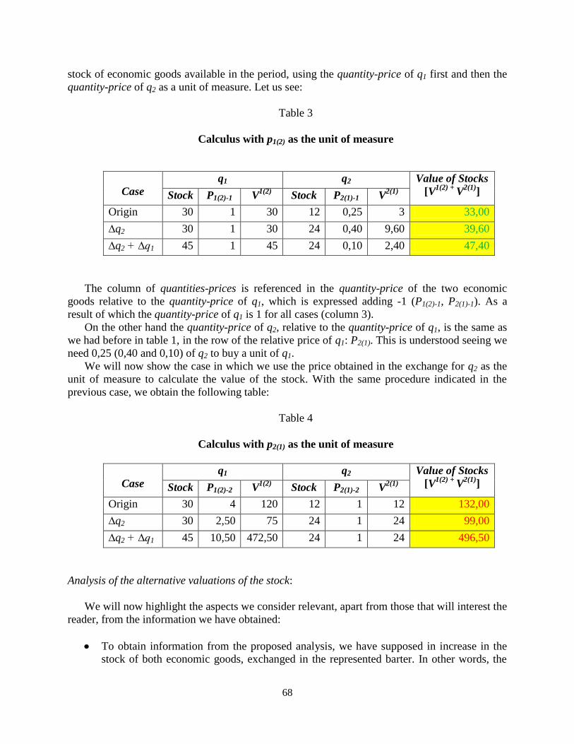
68

stock of economic goods available in the period, using the quantity-price of q1 first and then the

quantity-price of q2 as a unit of measure. Let us see:

Table 3

Calculus with p1(2) as the unit of measure

Case

q1 q2 Value of Stocks

[V1(2) +

V2(1)

] Stock P1(2)-1 V1(2)

Stock P2(1)-1 V2(1)

Origin 30 1 30 12 0,25 3 33,00

∆q2 30 1 30 24 0,40 9,60 39,60

∆q2 + ∆q1 45 1 45 24 0,10 2,40 47,40

The column of quantities-prices is referenced in the quantity-price of the two economic

goods relative to the quantity-price of q1, which is expressed adding -1 (P1(2)-1, P2(1)-1). As a

result of which the quantity-price of q1 is 1 for all cases (column 3).

On the other hand the quantity-price of q2, relative to the quantity-price of q1, is the same as

we had before in table 1, in the row of the relative price of q1: P2(1). This is understood seeing we

need 0,25 (0,40 and 0,10) of q2 to buy a unit of q1.

We will now show the case in which we use the price obtained in the exchange for q2 as the

unit of measure to calculate the value of the stock. With the same procedure indicated in the

previous case, we obtain the following table:

Table 4

Calculus with p2(1) as the unit of measure

Case

q1 q2 Value of Stocks

[V1(2) +

V2(1)

] Stock P1(2)-2 V1(2)

Stock P2(1)-2 V2(1)

Origin 30 4 120 12 1 12 132,00

∆q2 30 2,50 75 24 1 24 99,00

∆q2 + ∆q1 45 10,50 472,50 24 1 24 496,50

Analysis of the alternative valuations of the stock:

We will now highlight the aspects we consider relevant, apart from those that will interest the

reader, from the information we have obtained:

To obtain information from the proposed analysis, we have supposed in increase in the

stock of both economic goods, exchanged in the represented barter. In other words, the

69

inverse explains the case of simultaneous decreases, and a decrease of q1 can substitute

the increase, to add to the increase we supposed first for q2. The analysis of decreases of

quantities supplied, instead of the increases proposed here, can be analyzed also

following the inverse path based on the same information we have presented. Mixed

combinations of increases and decreases of quantities will shed the same light.

We can see that, according to the price we use as a unit of measure, or of absolute relative

“pure” prices, the final figure reflected by the value of the stock is completely different,

let us see:

496.50 ≠> 256.50 ≠> 47.40 99 ≠> 72 ≠> 39.60 132 ≠> 55.50 ≠> 33

Which indicates that the figures are not only different, but they are also greater if we use

smaller relative unit quantities-prices (that is why we have included the composed

symbol ≠>) and vice versa.

We must bear in mind that here we have compared values of each of the three situations

according to each method chosen for the valuation, not of the values of each of the three

situations “within” each method of valuation, a case that we will analyze below.

It is very important to highlight what happens in the case of the value 99 of table 4, in

reference to the fact that: the increase in quantities does not necessarily imply an

increase in the value of the stocks in all cases.

256.60 (for 45 + 24 = 69) > 72 (for 30 + 24 = 54) > 55.50 (for 30 + 12 = 42)

47.40 (for 45 + 24 = 69) > 39.60 (for 30 + 24 = 54) > 33 (for 30 + 12 = 42)

496.50 (for 45 + 24 = 69) > 99 (for 30 + 24 = 54) < 132 (for 30 + 12 = 42)

THE EXCEPTION: this “exception” expresses the case in which the decrease of the

quantity-price of the good used as unit of measure, due to the increase of its stock, was

relatively larger than the increase produced in the quantities of the stocks. Here the

quantity-price of the economic good chosen as the unit of measure fell 37.50% (2.50

now, added to 4 before), versus an increase in the quantity of units of the stock of 29%

(54 units now, added to 42 before). Then, the increase of the weight valued between

quantities-prices and “physical” quantities, resulted in that the increase in the “physical”

quantities did not compensate for the decrease in the quantity-price used for weighting.

This “exception” confirms TET, since neither the quantities-prices ―Price Wicksell

Effect? ― nor the “physical” quantities ―Real Wicksell Effect?― by themselves can

explain the economic value ―explained to consider complementary. A situation we will

have the opportunity to corroborate further on, as the decrease in the quantity-price of the

unit of calculus will reflect the decrease of the calculated value of wealth. Which would

“imply contradicting” that, ceteris paribus, an increase in the stocks of economic goods

benefits demand.

70

This situation produced great confusion in the theoretical developments of the twentieth

century, very well represented by the debates between Hayek and Keynes (29)

about what

rises and falls of prices meant for the economy. Keynes maintained that price rises were

what gave the impulse for the profit companies needed to do business, and Hayek

rejected this. Here we will show if one of them was right and why.

The figures we have obtained in this case only show that an increase in the quantities of

the economic good used as a unit of measure ―which implies a decrease of its quantity-

price― can imply a lower valuation of total wealth. This situation will be seen in its full

dimension when we study generation and destruction of wealth, and it will corroborate

the exercise we have presented.

We must bear in mind here we have compared values from each case in relation to a

system of stock valuation, one with quantities-prices and no unit of measure, and two

with relative prices with a unit of measure. This is the method used in everyday life, and

that is why the “exception” case is important.

Value: it is important to bear in mind we have used the expression of greater or smaller

value in the sense of a greater or smaller number. This is so insofar as we can use one or

another price to value both economic goods.

Let us see another very important conclusion resulting from the exercise on the issue of

value. To this effect we analyze the final result of the three proposed options, and concentrate on

the percentage variations of the value of the stock for the period, according to each type of

valuation, knowing the quantities of goods have varied equally for the three methods. Let us see

table 5.

This table was built considering:

The first two columns represent the percentage variations of the proposed increases of the

stocks, in the stocks of each economic good.

The other three columns, expressed in values obtained for each one of the three cases,

according to the unit of measure adopted, for the first pair of columns that expressed in

pure quantities-prices with no unit of measure, expressing in its first column the value

calculated for each situation, and in the second the percentage variation compared with

the previous one. The two following pairs of columns were built with the same criterion,

one considering the quantity-price of q1 as the unit of measure, and the other the price of

q2.

A fall of the quantity-price of the unit of economic measure

leads to a fall of the figure of the calculated value of wealth.

71

We can observe the complete lack of harmony between the percentage variations of

quantities, and the percentage variations of values. And there is a negative percentage

variation in the case of 99.

This table is presented to reiterate, once again, that it is essential to say what unit of measure

is being used for valuation in economics, since as we can see we obtain completely different

figures with one or another. Nevertheless, we reiterate also that we do not find here the

difference with the units of measure of physics (you also get different figures if you measure

with meters or yards), instead it is in the variation you find in economics due to the use of

one unit of measure, the price of one economic good ―i.e., in economics the yard and the

meter vary, a circumstance that must be taken into consideration to be able to calculate.

Table 5

Different values for the same stock

% ∆ Stocks

Stock value with unit of measure:

P1(2) y P2(1) P1(2) P2(1)

q1 q2 V1(2)

+ V2(1)

% ∆V(a)

V1(2)

+ V

2(1) % ∆V

(a) V

1(2) +

V

2(1) % ∆V

(a)

33 100 256,50 256 47,40 20 496,50 401,00

100 72,00 30 39,60 20 99,00 -25,00

55,50 33,00 132,00

(a) Represents the percentage variation compared to the previous state: ∆ 256 % is

the percentage increase of 256.50 over 72.

So we see:

General variations: it is important to stress that when we observe the final result of the

exercise we see that not only the exchanged amounts change but also the final stocks.

Economic calculus: from all this we deduce that it would be very useful to be able to

define an economic good as a unit of measure for all exchanges, because it is clear that:

a) If we can use three forms of valuating the exchanges, for each pair, it is easy to

conclude that in a community with millions of exchanges of millions of economic

goods, it is impossible to generate useful information. This complexity led mankind

to use a common unit of measure to value all economic goods, as we shall see.

72

b) We can understand then why human beings discovered spontaneously the economic

good of common use for exchanges, so that its quantity-price would serve as the

generalized unit of measure for valuations or economic calculus.

c) We can also understand the preoccupation with respect to a “fall” of the price of the

economic good used as the unit of measure, considering what it implies for the

valuation of the stocks of economic goods. A situation that is not considered in

currency policies to which we will refer.

d) We can understand that an increase of the value of the unit of measure is not a

problem, on the contrary, since it avoids the “currency veil”. I.e., the reference to the

“barbaric relic” in reference to money currency was very unfortunate (we are

referring to Keynes comment on gold as currency).

The effect of the closed box: Its use allowed us to understand that the variations of the

quantity-price of goods does not alter in proportional or homogeneous form the value of

economic goods; that is in fact impossible based on the laws of marginal diminishing

utility and returns underlying the law of exchange.(30)

In accordance with the measurements of the other sciences, the use of different units of

measure produces different “figures” with the same objects; by simple effect of

multiplication the figures are greater according to the unit of measure used being greater,

and vice versa.

To this effect it is sufficient to observe that if in a period of time we value Argentine

wealth considering its peso as the unit of measure, as time goes by the figures will be

greater here then what we obtain if we use the American dollar or the euro as the unit of

measure, and this is so considering the quantity of Argentine pesos supplied was

exponential compared to these currencies. A situation that is referred to with the concept

of “currency devaluation” or “variations of the exchange rate”.

What is distinctive in economics is that the valuation will be smaller the greater the

amount of the economic good used as the unit of measure, given that the greater the

amount of the economic good chosen as the unit of measure, ceteris paribus, the smaller

the price after the increase. And vice versa.

IMPORTANT: as the stock of units of the economic good used as the unit of measure

increases in time (ceteris paribus) its price decreases along with the valuation of the

stocks, and vice versa. IT IS NOT THAT THE QUANTITIES-PRICES OF OTHER

GOODS RISE, an unfortunate use of language under the title of “general level of prices”.

Conclusion on the arithmetic calculus of the benefit of demand.

It is not appropriate to express figures of value without indicating what economic good the

units in stock refer to, and to what unit of measure the valuation calculus refers to. In the same

sense that we do not simply say 5 if we wish to refer to bread and 5 kilos. It is only with this

qualitative data (bread), the unit of measure kilo and the quantity 5, that we know we are talking

of 5 kilos of bread. In the same manner we say those 5 kilos of bread “are worth” 50 monetary

73

units ($). We need to refer first to the quality; for economics here it is 5 kilos of bread are worth

$ 50, interpreting “worth” in the sense that 5 kilos of bread are exchanged for 50 currency units.

Based on the example of barter, we see the need to continue developing the economic

causality chain to be able to explain further. But we do this fully confident, since we know we

must not abandon the a priori logical deductive chain of causality. On the contrary, it shows us

man must find a solution to calculus with the adoption of a unit of measure, knowing what this

will imply. Even so, TET’s posture is ratified in the sense that economic calculus is feasible

where quantities-prices are generated, even if they are not in quantities-prices-currency, since

barter also generates them, a theoretical observation on Mises we made based on TET.

What we have developed up to this point will be of extreme importance to explain the

economy as we shall see. We expressly ask that the reader concentrate on understanding the

score of the symphony presented by the a priori logical deductive causality chain we saw up to

here, since it is the same symphony we will continue to observe.

Yes, we have seen economics up to here, but sharing the same basics as the double entry

accounting techniques. The truth is that economics and accounting share the same basic

fundamentals of causality, the fundamental causality of economics ―need → economic

goods―. That is why for Mises and for us it is very easy to say that accounting is the model for

economics, complying with the necessary and sufficient conditions to explain the economy.

We cannot leave this part of the development, since it is foundational for what follows,

without reiterating that the conclusions we have reached up to here are based on applying the

marginal laws of utility and returns, both diminishing. A situation which on the one hand is

guarantying fidelity to the method of the a priori logical deductive chain of causality,

uncontaminated with other developments that could alter the clean use of these foundational laws

of economics, since they are primitive terms that substantiate the fundamental economic

causality demand → supply.

When comparing the conclusions obtained geometrically and arithmetically we can conclude,

ceteris paribus, that the increase in the quantities of stocks of economic goods supplied implies a

benefit for demand, though the case of the 99 value could induce us to think we are in the

presence of a non benefit.

The reflection in the preceding paragraph is what has interested the economists of the

twentieth century, and they based their theories on this issue to explain the consequences of the

variations of quantities-prices of the universal unit of measure (quantity-price-currency), and its

consequences for wealth distribution and unemployment of labor and available resources in

general. This work ends with an explicative model which will allow us to corroborate the

enormous importance of classifying the types of currencies a community can choose WHEN

CALCULATING ―in both this quantity-price is the universal measure unit ―, since the use of

one or the other has opposite effects and can lead to devastating consequences ― the laws that

govern quantities-prices of money in time are different from the laws that govern the

quantities-prices of credit.

QUANTITY-PRICE, VALUE, AND THE BENEFIT OF DEMAND

Therefore, when measuring the economic benefit of demand, it is of great importance to

understand the relevance and consequences of the necessary use of a variable unit of measure in

time. Thus, the calculus of the total value of wealth is determined based on weighting the

74

physical units of each economic good by the marginality they contribute to the price, which is

relative to the good for which it is exchanged.

It is important to consider how we have treated the specific case of the exchange of an

economic good for another, which allowed us to produce the economic calculus of the value of

wealth in the primary phase of barter, an achievement of enormous magnitude, no matter how

trivial it might seem. In other words, we have adopted the alternative of going from the simple to

the complex, instead of the traditional method of explaining based on currency, and supposing

that without currency we cannot calculate. We have proven that without currency it is possible to

calculate, considering as such the process of valuing based on quantities-prices that derive from

exchange, if we are in the presence of barter.

It is also known that man discovered the way to go beyond the primitive phase of barter,

using currency. The very good news is that to study the phase of currency we need not alter what

we have developed in the least, since we only need to value all economic goods considering their

quantities-prices relative to the quantity-price of currency. Thus we can compare the values of

all economic goods given the common factor included when using a unit of measure of universal

use. Which we will logically do.

The reader that has encountered the external theoretical struggle considering if a rise or fall

of prices is beneficial,(31)

can now find a concrete answer, since we now understand how

marginal magnitudes (relative and temporal, as everything marginal) and total magnitudes come

into play. On the other hand, he will have been able to see what effect the use of different

systems of valuation has, and the enormous importance of the rise or fall of the quantity-price of

the economic good used as the unit of measure, being the method adopted by advanced

communities that have gone beyond the phase of barter.

Given that the increase of quantities (ceteris paribus) implies efficiency has produced results

―appearing as the underlying motivation the need to cover the shortages that explain human

economic action― since there is a greater benefit of demand, we can conclude we are in the

presence of more benign consequence of the law of diminishing returns, due to the efficiency

attained thanks to its incidence. In other words, efficiency (derived from capital, technology,

knowledge, discovery, productivity, etc.) must be the prow of all societies. Institutions opposed

to efficiency ―bureaucracy― harm humanity, which makes us think it should be considered a

crime against humanity, since it causes harm to life itself.

In the continuity of the causality chain we have been developing, important for what is to

follow, it will be useful to retain these conclusions:

1) Unit of measure for valuing wealth: the calculus of the value of economic goods is based

on the relative quantity-price of the economic good chosen as the unit of measure.

2) Unit of measure variable in time: being the unit of measure of economic calculus a price,

we immediately deduce the impossibility of it being constant in time. Especially

considering it is the reference quantity-price for all other quantities-prices (except its

own). A trivial circumstance in our development, but it has been and still is one of the “so

many inconsistent” problems of economic theory and practice. I.e., it is not prudent to

equate the function of the unit of measure in economics, with the units used in physics,

apart from the fact that in that case there is also no constant unit of measure (it is

considered constant disregarding small differences).

75

3) Currency veil – Consequences of calculus with a variable unit of measure: precisely the

variation of the price of the economic good used as a unit of measure is of transcendental

importance in calculus, since it is the multiplying factor with which humanity values

wealth and makes all economic decisions. To that effect we only need to bear in mind the

case of 99, which presents lower figure of value of wealth (ceteris paribus) with the same

or greater quantities of stocks of economic goods (wealth). In short, calculus with the

variable unit of measure explains that case 99 is no exception, but a consequence with an

explainable causality, here duly explained and clarified, that allows us to eliminate the so

called “currency veil”, that would be a veil if we could not explain it.

4) Selection of the unit of measure: in terms of what it means to choose an economic good to

be used as the unit of measure (currency), a complete and precise currency taxonomy is

of transcendental importance.

Given what we have seen, we can discover the transcendental importance of the

taxonomy proposed by TET when classifying currency: it is very different for the

economic good currency to be part of the equation An = PNn, composed of stocks of

present economic goods (with no risk for what is pending for the future), from currency

belonging to the equation Crn = Dn, representing exchanged economic time, which is

subject in turn to the relativity of other economic goods. Let us see the classification of

currency we adopt, according to the Theory of Economic Time:

Money currency: subject to the relativity of quantity-price.

Regular-credit currency: subject to the relativity of quantity-price + the relativity

of indirect materialization (being credit).(32)

Irregular-credit currency: subject to the relativity of quantity-price + the

relativity of indirect materialization (being credit) + the uncertainty of not

specifying the indirect materialization.

We reiterate that it is of transcendental importance to see if currency is money or credit,

if the credit is regular or irregular, given that the quantities-prices each one forms in

exchanges obey completely different laws. Of extreme importance, derived from the fact

that it is the universal economic unit of measure.

5) Generating or destroying the value of wealth: another central aspect when classifying the

different types of currencies is linked to the function of preserving value. TET firmly

states it is not an exclusive property of currency, since all economic goods exist because

of the value assigned to them, or they would not be economic goods ―more proof that

currency does not merit a special theory. Nevertheless, it is curious to appreciate that the

value of currency is a property that should be recognized even more in currency,

considering it is assigned the function of acting as a unit of measure, and we know it

guides the calculus of value in wealth in economics, i.e., the alteration of its quantity-

price implies altering all other calculus. In other words, the rise in quantity-price of

currency implies greater value of the wealth calculated, and the opposite implies less

value. All which tells us that the alterations in the quantities of currency imply generating

76

or destroying the value of the wealth calculated. As the reader can observe, the more we

progress with our work, so much more unfortunate the expression “barbaric relic”

appears to be.

It is very important for the reader to remember this section, since it will be very important

for the following developments:

Economic value is calculated with a variable unit of measure

We end this section saying the circumstance of using the price of an economic good as a unit

of measure for calculations of the value of wealth does not authorize us to forget that the

quantity-price of the economic good used as a unit of measure is still a quantity-price, generated

in exchanges where the good in question participates, just like any other economic good. I.e., we

cannot consider an absolute quantity-price or a quantity-price that is not relative, because of the

fact that it is used as a unit of measure to calculate the value of wealth.

Forgetting what is in the preceding paragraph is the reason why theory did not understand

what happened in the event presented with “case 99”. That error led to think that “case 99”

implied the destruction of wealth as a stock of economic goods, when it expresses the value of

wealth using as a unit of measure the decreased quantity-price of an economic good. But if we

compare it with the two other possibilities of valuation ―relative prices without a unit of

measure or the quantity-price of another economic good as the unit of measure― that

circumstance did not occur. As a consequence, with the fall of the price that is the unit of

measure, what we have is a destruction or fall of the value of the wealth calculated with that unit

―a situation that does not occur with the use of the other two methods―, of which we will

analyze the consequences.

QUANTITY-PRICE THEORY

Evidently what we have developed allows us to shed much light on price theory. To that end

we present a brief summary of its evolution, and how our chain of logical deductive causality

beginning with Gossen’s three laws can be presented as a synthesis.

Classics (Theory o objective value): they said prices were determined by costs, and so

these end up determining prices, and at the same time they accepted that supply and

demand determined prices. It is what is known as the classical vicious circle ―that we

represent: cost ↔ price ―, based on it classical theory could not explain the “price

phenomenon”. It is important to recognize the influence of David Ricardo in this, above

all with his analysis on diminishing returns.

The classics’ argument was that prices “derive from things”, i.e., they were objectified in

economic good. The extreme case was Marxist dialectic materialism.

Marginalists (Theory of subjective value): with the advent of the theory of subjective

value at the end of the nineteenth century the classical vice was solved, since prices arise

77

from the subjective valuation of the participants in the market, not the costs, aspect that

has its explanation in imputation theory, discovered by Menger and explained by Hayek.

Theory of Economic Time: it proves the laws of supply and demand are unnecessary to

explain the formation of prices, our EP

since they are explained by the joint incidence of

the laws of diminishing marginal utility and the law of diminishing returns. In other

words, the curve of demand is the representation of the behavior or functioning of the law

of diminishing marginal utility (the curve of need or Gossen’s curve), and the curve of

supply is the representation of the behavior or functioning of the law of increasing effort

(diminishing returns).

The Theory of Economic Time (TET) clearly states that the well known laws of supply and

demand ―foundations of the current theories― are in truth the observed consequences of the

“natural” laws of diminishing marginal utility and diminishing returns. This is very important,

since legislating on quantities-prices is intervening in the functioning of these laws, it is like

legislating on the law of gravity and its consequence are usually catastrophic, within the sphere

of crimes against humanity. A situation that can be avoided legislating only one sentence saying:

it is forbidden to alter the free functioning of the laws of marginal diminishing utility and

returns.

In reference to the link of the theory of Quantities-prices to the theories of value and the

functions of the same, let us remember emphatically the central role we have given the temporal

function of quantities-prices here, insofar as they define the moment in time of the end of

exchanges and the beginning of stocks, overshadowing the traditional approach of focusing on

the explanation based on exchange (33)

– we suggest studying, not just reading, note 33.

78

CURRENCY

Before continuing with the study of the quantity-price of the unit of measure currency, it is

very important to reflect on the consequences what we have seen and concluded up to this point

has for the theory of quantity-price.

THE ECONOMIC GOOD CURRENCY IN EXCHANGE

The appearance of exchange showed the presence of a need, overcoming the routine, costly,

and bothersome phase of barter. Once again human action was mobilized to overcome a state of

dissatisfaction, which originated the discovery of currency. We can ratify currency was an

efficient answer to a need that showed a very high marginal effort level (level of the curve of

supply).

The Theory of Currency in TET, defines currency as the economic good that satisfies the

need for liquidity, (34)

―without excluding other functions― illiquidity being what is

characteristic of the phase of barter. From this definition derive the qualities that an economic

good must have to reach the status of currency, and the functions it will have in the economy. (35)

Once it is understood that currency is an economic good (that satisfies the need for

liquidity), we can include it in the a priori logical-deductive causality reasoning we have been

developing and show how the quantity-price of currency is determined in an exchange, and in

turn how economic goods exchanged for it define their quantity-price compared to the quantity-

price of currency. In other words, the study of currency does not need special developments to

apply to it the theory of subjective value.

THE QUANTITY-PRICE OF THE ECONOMIC GOOD CURRENCY

Given the nature of the economic good currency, we can analyze it within the development

we have been producing. (36)

Thus we present chart 13.

In the ordinate we have represented the stock of an economic good that is not currency (q),

and in the abscissa we have represented the stock of the economic good currency (m). We have

represented the curves of supply-demand of both goods that seen from the “producer” of

currency are Dm(q) y Om(q) respectively, and its prices expressed in quantities of another good: the

price of the economic good currency expressed in the economic good q appears as Pm(q), and the

price of the economic good q expressed in the economic good currency Pq(m). We reiterate that:

Om(q) = Dq(m)

Dm(q) = Oq(m)

Where:

Om(q) is the supply of m for the demander of q

Dq(m) is the demand of q for the supplier of m

Dm(q) is the demand of m for the supplier of q

Oq(m) is the supply of q for the demander of m

79

This important conclusion is what allows us to work in the real world of quantities-prices

observed in the market, which indicate ―of all quantities that make up the stock― the end of

exchange and the beginning of stocks.

Chart 13

The quantity-price of currency

13

We should remember we find here a rectangular closed box, whose sides have the length of

the quantity of the economic good currency (mst) in the case of the abscissa, and the quantity of

the other economic good (qst) in the ordinate.

For expositive reasons, from now on we will refer to the quantity-price-currency Pm(q)

simply as pm, knowing it is expressed in the quantities of other economic goods with which the

economic good currency is exchanged. In the same manner we could represent Pq(m) simply as pq,

as the price of the other relative economic goods expressed in terms of the price of currency,

whose quantities-prices are also relative.

We deduce then that when we express that a unit of the economic good q1 has a quantity-

price of 5 pm, or $ 5, we are saying that 5 units of the economic good currency (m) were supplied

to buy a unit of q1. Which, seen from the side of the quantity-price of the economic good

currency tells us the quantity-price of a unit of the economic good currency (m) is 0,20 of a unit

80

of q1 (0,20 is the quantity-price of q1 in terms of the currency). Table 6 shows us the analysis we

have carried out:

Table 6

Table of (relative) quantities-prices

Mathematically it is explained by

1q = 5m

1m = 1/5q = 0,20q

As you will see, it is not necessary to be a PHD in mathematics to understand the price of the

economic good currency expressed in currency [Pm(m)]. Specifically, the price of a unit of the

economic good currency (1m) expressed in currency is expressed by Pm(m) = 1m = m.

VARIATION OF THE QUANTITY-PRICE OF THE ECONOMIC GOOD CURRENCY

We will now study the consequences of a variation in the quantity of currency, more

specifically the increase in the quantity of currency supplied in a period of time, since that is the

most common event we can observe in our times of credit-currency, different from money-

currency. In turn the opposite process ―a fall in the stock of present currency supplied in a

period of time― only requires to be read in the opposite sense to the one presented here, i.e.,

instead of determining point E1 based on the original position of point E

0, we must consider the

path from point E1 to point E

0.

Let us see chart 14, where we suppose an increase in the supply of currency in the period,

from the original 30 to 45, which is shown in the passage of the supply drawn on the abscissa

with a black scale, to the abscissa with the scale drawn in green. All this derived from our being

in the presence of the closed box of exchange (where supply of q is kept at 12 units).

Components and analysis of chart 14:

With black lines we represent the original box of exchange of economic goods, the

currency (m) in the abscissa and q in the ordinate, representing the economic goods that

are not currency. The stocks are determined by the scale in black, 30 and 12 unites

respectively.

We add the new state of stock of m, that now, instead of 30 units, is 45, 50% more units.

Economic good

Relative

economic good

Relative unit

price

.q .m 5 m

.m .q 0,20 q

81

Due to the preceding, we now add a new scale of the abscissa where we present the new

stock of currency, which is drawn in green.

Also due to the same reason we draw the new curve of Offer (supply) of m, we identify in

green O1

m(q), maintaining the curve of Demand D0

m(q), since the stock of q, supplied in the

period, has not varied.

Chart 14

Variation of the quantity-price of currency

In this manner we obtain a new point E, represented by E1 that identifies the new

quantities-prices, now two units of q are exchanged for 30 units of m, different from E0

where 3,50 units of q are exchanged for 16 units of m. From where we deduce:

a) The increase of the stock of a good, ceteris paribus, implies a decrease of its quantity-

price relative to the other, which implies an increase of the price of the other relative

to the first.

82

b) The variations of quantities-prices are not proportional to the increase in the quantity of

the good. I.e., if we increase 50% the stock of m it does not imply its price will fall a

third. Once again the closed box of exchange proves the non-existence of a homogeneous

or linear behavior.

c) The alteration of the quantity supplied, reflected in the passage from E0 to E

1, implies

altering the quantities exchanged and in stock of all goods. Which indicates that the

increase of supplied quantities in this case of a good, ceteris paribus, implies variations in

the quantities exchanged and/or in the stocks of both products, but one at a higher

quantity-price than before and the other at a lower quantity-price than before.

d) Additional conclusion: the preceding allows us to infer that with the perspective of the

economic good currency loosing value, human beings will not want to keep it, making it

circulate in exchanges, opting for economic goods that they consider will not lose relative

price. The reader can decide to call this behavior Gresham’s Law, we simply say that the

law of exchange implies selling an economic good with a higher quantity-price if we can

carry out the same exchange for one with a lower quantity-price, with which we are

referring not only to the economic good currency, but to all economic goods that are

exchanged. Thus, Gresham’s Law does not add or subtract from the more general law of

exchange (it implies the marginal laws) that governs all economic goods –once again we

corroborate apparently that currency does not justify a special theory.

If you observe in the study of the variations of the quantity-price of currency here presented a

similitude with the conclusions we have obtained when analyzing the variations of the relative

quantities-prices of any good (preceding charts) you will be right.

If you are wondering why we have included this section to study the variations of the

quantity-price of currency, since it is a replica of what we have seen in previous charts, you will

be right.

Conclusion: what is known as the quantitative theory of currency implies referring to an

economic order where the marginal laws of diminishing utility and returns, and the law of

exchange derived from them, are not valid, since the observation of these laws produces opposite

results to what that theory postulates. But if an economic theory does not derive from the validity

of the marginal laws of utility and returns and the law of exchange derived from them, we hope

we do not offend anyone if we say it does not belong to the economic sphere.

QUANTITIES-PRICES RELATIVE TO THE QUANTITY-PRICE OF THE ECONOMIC

GOOD CURRENCY, AS A UNIT OF CALCULUS

We saw that quantities-prices are units of measure referenced in another economic good,

which leads us directly to the enormous advantages for exchange and all the economic calculus

man has to produce, to be able to have an economic good as a general reference, having point EP

as the “agent” of the main information. We need not continue, and can say this economic good is

currency, which is the reason why the prices of all other economic goods are relative to the price

of the economic good currency, representing the currency quantities-prices of economic goods.

83

We already saw the huge power of quantities-prices for calculating, which in economics

implies:

1) The moment when exchanges cease.

2) The moment when stocks are generated.

3) Quantitative information making the subjective value underlying its formation visible.

4) The process of valuation of wealth, calculation performed with a variable unit of

measure.

Thus, it is understandable that we would be much better situated to carry out economic

calculus, that allows us to value, if we use the quantity-price of a good of generalized use, which

would allow it to be a universal reference since it is known by all, and in that manner we could

compare all the calculus we have made.

Things being what they are, it is no chance that we have formally introduced this section

―as simple and elementary as man can perceive it in his economic life― in the a priori logical

deductive chain of causality we have been developing. Yes, currency as the unit of measure of

generalized use in economic calculus will become a relevant link in the explanation of the social

economic evolution we are forging.

84

ECONOMIC CALCULUS

Since we have already referred to the importance of economic calculus, which in economics

consists of valuating wealth multiplying the “physical” quantities of an economic good by its

quantity- price ―relative or expressed in quantities of the economic good by which its quantity-

price was determined in exchange―, and added to the importance of referring the valuation of

all economic goods to the quantity- price of the economic good of common use, the currency, we

directly initiate the economic calculus of goods expressed in the quantity- price of the economic

good currency.

It was Ludwig von Mises, in this aspect continuing the legacy of Carl Menger, who stressed

the importance of prices, since they allow economic calculus. More precisely, Mises stressed the

relevance of prices of economic goods expressed in the economic good currency, our pq(m), of

which we have highlighted with great emphasis its particularity in economics of not being a unit

of measure that is constant in time. That is why the only thing constant we can obtain with an

economic unit of measure is the specific quality of the economic good chosen as currency, an

aspect that makes its fungibility (37)

― first and fatal flaw of paper money― relevant in

economics as an essential property of an economic good that will acquire the status of currency.

In reference to Mises posture, we believe it prudent to stress what to our understanding he

pretended to say, or what we interpret as the central aspects of economic calculus, which we

understand he would positively accept; let us see:

The theory of subjective value is what explains the fundamentals of the human action of

exchange, insofar as the value which each human being gives economic goods is what

leads him to better his situation previous to the exchange.

Quantities-prices are the factual sign of subjective value. Prices are the tools that allow

us to limit the theoretical concept of subjective value and make it observable. It is in this

manner that quantities- prices formed by the market allow the concept of value to be

included in wealth ―generated by effort of labor, specialization and distributed under

law of exchange―, which man does weighting the physical units of the economic goods

by the quantities-prices observed in exchange, since these are the visible expressions in

fact of the subjective values that drive the human action of exchange. It would be more

correct to say that value is wealth itself, since we cannot conceive an economic good

(wealth) with no economic value, by the axiom of the positivity of prices of TET (p > 0):

prices are always positive by definition of quantity-price.

Economic calculus only values wealth, knowing that wealth is the value of economic

goods, which for calculus are weighted by the relative quantities-prices of other

economic goods.

Calculating (valuing) allows us to compare, both the stock and the variation of wealth, be

it of one agent in time, or different agents at the same time.

Economic calculus allows us to value both the creation and the destruction of wealth, and

its inseparable distribution, as we shall see.

85

The benefit of demand (profit) is to add value, which derives from weighting quantities

and prices.

Having produced this very important conceptual summary of the basics of economic

calculus, we continue with the development of our chain of thought.

Of all the quantities-prices formed in exchanges, those of all the goods expressed in the

economic good currency [(pq(m))] are essential, since it is the relative reference of all quantities-

prices. In other words, of all exchanges, that which is constantly carried out “for” the economic

good currency is what is taken as reference for all economic calculus, as is shown in table 7.

Table 7

Quantities-prices of the economic goods expressed in currency

Quantities-prices expressed and relative to the economic good currency (m)

1q1 1q2 1q3 1q15 1m 1qx

5m 0.2m 8m 10m 1m 40m

Table 7 represents the information obtained from the exchanges carried out in certain spatio-

temporal points. In turn, here we have simplified the information, since we have expressed

everything in units of each economic good, even though exchanges are not carried out in that

manner.

It is important to observe that the quantity-price of 1m expressed in m –the Pm(m) we have

presented before― has not derived from an exchange, instead it is presented for a didactical

symbolic reason.

In this manner we arrive at the fact that the quantity-price of a unit of the economic good

currency is what humans adopt as the unit of measure for their economic calculus. (37)

Having

reached this point we can now approach with scientific rigor the a priori logical deductive

causality that governs economic calculus.

86

WEALTH

― CALCULUS AND DISTRIBUTION ―

We are now ready to calculate wealth, both in its generation (Adam Smith) and its

distribution (David Ricardo).

STOCK AND CALCULUS OF WEALTH

Based on the concept of wealth as the totality of economic goods of an owner at a certain

spatio-temporal moment, we proceed to integrate the determinants that generate wealth, which

we know what they are and how they interact:

Elements of the fundamental economic chain of causality

Man.

Economic goods (stock of wealth)

Laws that govern the connections between the elements in the fundamental chain of

economic causality

Law of diminishing marginal utility

Law of increasing marginal effort

Law of diminishing returns

As we have expressed before, to obtain theoretical conclusions that we can represent with

visible variables, we will use the idea expressed in the area α of the stock of wealth developed

above, since it is feasible to produce an inventory of the quantities of existing economic goods

(qx) at a certain time, to which we assign a number for economic calculus multiplying it by the

price informed by exchanges. (38)

And as we saw, for economic numbers to be understood by

everyone, it is adequate to use in the multiplication, of all the prices of each economic good that

form wealth, the quantity-price-currency that is relative to the economic good currency.

Robinson’s stock of wealth

We present charts 15 (a) and 15 (b) of Robinson’s stock of wealth.

In chart 15 (a) we have represented Robinson Crusoe’s wealth in the solitude of the island,

without quantities-prices, I.e. while there is no exchange that generates, therefore we only have

quantities. In this manner the sum is inadequate since we are adding pears and apples and the

total of units does not tell us anything useful for economic calculus.

In chart 15 (b) we suppose Robinson integrated in a society of individuals that exchange, and

that originates quantities-prices of goods, quantities-prices that are relative or expressed in units

of the economic good currency, since this community uses it and has gone beyond primitive

barter.

87

Chart 15

Stock of Robinson’s wealth

Without quantities-prices With quantities-prices-currency

We obtain the stock of wealth in both cases, expressed in the following summations:

Robinson with quantity

Ʃ qxst (x from 1 to z)

Robinson with quantities-prices

Ʃ qxst px(m) (x from 1 to z)

It is very important to remember that the surface that determines the charts of stock of

economic goods, represent Robinson’s total wealth in a specific spatio-temporal moment, i.e.,

they can be measured ―stock inventory with quantities-prices-currency, and the exchanges of a

period can be measured in the same way. In other words, the quality of the representation of

Robinson’s wealth depends on the quality of the data obtained by the observer.

Stock of wealth of “n” owners

We now present the chart of stock of wealth (α) of n owners that make-up the economic society,

calculated in prices relative to the economic good currency. Let us see chart 16:

88

Chart 16

Stock of wealth of “n” owners

We have represented the stock of wealth of an individual and of a group at a precise spatio-

temporal moment, based on the fundamental economic equation man (n) → economic good

[qxstpx(m)]. Starting from the stock of wealth we have obtained based on the fundamental

axiomatic economic causality: owners ↔ economic goods (expressed in relative-unit prices of

the economic good currency). Now we are going to determine how that wealth is generated and

distributed, limiting the analysis to the economic laws of marginality we have seen.

Stock of aggregate wealth of “n” owners

Chart 17 shows how the stock of wealth grows as we add-aggregate the wealth of the individuals

that are the owners. Let us see:

89

Chart 17

Stock of aggregate wealth of “n” owners

Starting from the origin we add to the right of the abscissa (owners) the stock of wealth (αn)

of each owner, expressed in quantities-prices-currency. So we have:

αn = Ʃ qxstn.px(m) (with n from 1 to n, and x from 1 to z)

where stn is the stock of economic goods (qx) of the n individuals.

Thus, the first rectangle (α1) is the summation of wealth of the individual 1, the summation of

the two first rectangles (α1 + α 2) gives us the joint wealth of individuals a 1 and 2, and so on to

the last owner, understanding as such the owner of that wealth. Thus we incorporate in the sum

the wealth (αn) belonging to individual n, obtaining the stock of wealth belonging to all owners,

with quantities-prices-currency relative to the unit used for calculus, the economic good

currency, that allows us to homogenize and make sense of the aggregate.

In algebraic terms we can express the wealth generated by n and owners:

∑ f(xi) ∆xi (i = 1 to n)

90

Property of the stock of aggregate wealth of “n” owners

According to the axiom of the biunivocal relation of TET (accounting expression of the

fundamental law of economic causality) owner → economic good, that in short means there is no

economic good without an owner nor an owner without economic goods, we can complete the

chart of the generation of wealth with the adjoining and complementary concept of wealth, and

so we have chart 18.

Chart 18

Property of the stock of wealth of “n” owners

In chart 18 we observe that what is indicated to the left of the ordinate is a mirror image of

what can be observed on the right. Since we know what is on the right is the representation of the

“currency” wealth of n owners, we only need to ask what the left side of the figure means, and it

is no more and no less than the indication of who the individuals owners of the wealth are. That

is why we have placed the letter D in the abscissa, to the right of the origin (accounting Debit

that shows the assets) and C to the left (the accounting Credit representing the property of the

assets). (39)

Completing the explanation, we observe each rectangle on the left is separated in two

components, the top part indicated with a D corresponds to net debt of the individual owner of

the wealth, and the bottom his Net Worth (NW). If you have detected that this is the use of

double entry accounting, you are right, and all this, given the axiom of TET’s biunivocal relation

91

economic good ↔ owner, which is the basis for the technique of double entry accounting in

accordance with the fundamental economic equation (man → economic good).

For a precise understanding of the net debt we have referred to in the previous paragraph, we

present charts 19 (a) and 19 (b).

Chart 19

Property of assets-wealth of present economic goods

In chart 19 (a) we have represented on the right the traditional assets of a company, composed of

what we have defined here as stocks of present economic goods (A = 7), to which we add the

credits (Cr = 3) making up the total of the accounting Credit with 10 monetary units, i.e.,

quantities of stock of economic goods multiplied by their quantities-prices referred to the

currency. On the left we have represented the same 10 units, expressed in what corresponds to

net worth (NW = 6) and debt (D = 4), i.e., the accounting Credit.

We are working with the graphic representation of chart 19 (b), since we are considering the

stocks of present economic goods (A = 7), which is equal to the net worth (NW = 6) plus the net

of debts and credits (D – Cr = 4 - 3 = 1).

We only need to reiterate that balance consolidation determines that in the final analysis we

always have A = NW, given that debts and credits are compensated, being always equal (in the

whole). But it is very important not to forget the incidence credit-debt has in economic affairs, to

which we will refer when we speak of the generation and destruction of wealth by society.

We have been able to show the stock of wealth of a group of individuals, in a homogeneous

manner with the use of a common denominator multiplier ―(m) in the multiples [pqx(m)]― we

have used to multiply by the quantities of economic goods that compose wealth.

Present goods versus future goods

Though we have already expressed it, it is important to reiterate a concept that has produced

many consultations when referring to present economic goods, or better said, when trying to

interpret credits, insofar as they are not present economic goods. The accounting consolidation of

credits and debits shows us precisely that not doing so would increase the quantity of economic

92

goods (to 10) without the correlative existence (since the stock of the exercise is 7, we would be

missing precisely the 3 that represent the credit = debt).

In the exposition we are developing it is clearly visible that the assets considered by TET are

those corresponding to present economic goods, insofar as credits have their future counterpart in

commitments by another agent, that is why in the consolidation they are not considered and we

refer to the equation A = NW. Nevertheless, we indicate the part of future economic goods, that

we represent with the dotted line D = Cr. (40)

In short, the credits (Cr) = debt (D) do not constitute present economic goods in our

analytical taxonomy. (41)

Thus, the way to be able to identify the non present economic goods is

as accounting does: being future commitments equivalent in their amounts, their joint

consolidation is pertinent for economics also. We stress that their consolidation does not imply

omitting them in the analysis.

Thus, credit-debt is an important factor for generating wealth, but it must not be considered a

present economic good, rather as a part of the analysis of the properties of economic goods,

insofar as the owner of a company uses the property of others to strengthen (leverage) his

companies’ development. We will have the opportunity to appreciate in its full magnitude the

beneficial effects of the expansion of credit-debt, and how pernicious its destruction is.

Curve of Stock and distribution of wealth of “n” owners

We can represent all this with curves, which we do in chart 20 in this section.

In chart 20 we present in continuous curve form the conclusions we have arrived at here. To

the right of the origin we observe the aggregate stock of wealth of the n owners at a certain time

and expressed in currency units (area An), and on the left its distribution according to its owners,

where we show the proportion of the same generated by debt (Dn= Crn), of the consolidated total

where NWn = An. The reader can imagine the curves as if they were connecting the middle points,

or vertices, from the origin of the surfaces α of the preceding charts.

The curve of debt is represented by a dotted line, since it is only there to show that its

presence contributes to generating wealth. However we work with consolidated figures of the

whole (An = NWn). This is very relevant, it is not possible to generate debt-credit without the

presence of a present economic good that originates it. The process of accounting consolidation

is solid proof of it. That is the reason for the dotted line, expressing its relative participation in

the present wealth but it does not add to “An = NWn”, that is only composed of present economic

goods.

The curves are symmetrical and opposed, the mirror image, which represents a parabola cut

off at the center, a geometrical expression of accounting double entry. In other words, the curve

of wealth generation is the parabolic representation of the evolution of wealth of a set of owners,

that since they can be represented by the accounting technique of double entry becomes a

powerful tool for economic observation.

93

Chart 20

Stock and distribution of wealth curve of “n” owners

Another important aspect of the parabolic expression obtained is that it ratifies the axiom of

economics postulated by TET, economic good ↔ owner, which is in turn the basis for

accounting double entry. On the other hand the parabola also ratifies that it is inconsistent to

separate ―in time or space― wealth from its distribution to owners, no matter if we are

referring to the stock or flow, its generation or destruction, aspects we will refer to now.

Conclusion

We cannot end this section we have called WEALTH, without presenting a more precise

definition or concept of this term, since it always refers to wealth as the stock of economic

goods, which is not wrong, because it points to economic goods (that have economic value). But

possibly it would be more precise to define wealth as:

94

This concept, and taxonomy of economic calculation, clearly states that in economics it

makes no sense to refer to entities with no value for man and yes that it refers to things with

value (economic goods). With which we include the two components of the fundamental

economic causality.

In turn this definition of wealth opens the door to the exceptional concept used in the

business world, “creating value is the businessman’s goal”. In other words, all the economic

world refers to value, entity which has at all stages of the human being (Robinson, barter and

currency).

Finally, this definition or concept of wealth is in line with the theory of subjective value,

since there are things that have no value and therefore are not economic goods. This will be very

useful when we present the practical model of economic calculus (appendix C), insofar as a thing

can have existed as an economic good at a certain moment t1, and continue to exist as a thing but

no longer as an economic good in the moment t2. When calculating the observable value

(weighted by its quantity-price-currency) of said economic good, it is evident that in the moment

t1 it will be multiplied by a quantity-price-currency hat is greater than zero, while in the second

moment, when there is no quantity-price-currency (because it is not an economic good),

multiplying it by zero will automatically exclude it from consideration. Therefore, by definition

of wealth it does not belong to the sphere of economic wealth. All this is in turn a ratification of

the axiom of the permanent positivity of quantities-prices we postulate from TET (p > 0).

Whealt is the value that te man assigned to the economic

goods.

Humans calculate economic value in quantities of

economic goods:

Quantities: Robinson phase without exchange.

Quantities-prices: Robinson phase of barter

exchange

Quantities-prices-currency: Robinson phase of

exchange with currency

95

WEALTH

― GENERATION AND DESTRUCTION ―

With the fundamental economic causality ―equivalent to the axiom economic good ↔

owner―, the marginal laws of diminishing utility and returns ―and the law of exchange derived

from them―, to which we can add the double entry accounting technique, we have developed

the a priori logical-deductive chain of causality that has allowed us to prove that the generation

of wealth and its distribution are complementary variables, two sides of wealth, one that shows

its configuration ―production structure and value― and the other its ownership, which indicates

that both components appear, persist and disappear concomitantly and simultaneously.

CURVE OF GENERATION OF WEALTH (by “n” owners)

With the necessary theoretical, technical and observational tools presented up to this point,

we will see they are sufficient to show how wealth is generated in a set of n owners. Chart 21 in

this section will allow us to appreciate this.

Chart 21 has been generated based on the following parameters (42)

:

1) In the abscissa we represent the owner (n) of the wealth.

2) In the ordinate we represent the available present wealth, generated in a period of time.

Said wealth is expressed by the value of the economic goods, which derives from the

quantities of economic goods (qxst) pondered by the quantities-prices-currency[Pqx(m)].

I.e., the wealth expressed in the ordinate appears through an accumulative addition of

individual wealth of the owners Ʃ qxst px(m).

3) The accumulation of wealth represented includes that belonging to the individuals that

generate greatest wealth up to that belonging to those generating the least wealth, all in

the period of time considered.(43)

This way we represent the wealth generation curve (g)

decreasing relative to the quantity of owners that form an economic society.(44)

The

wealth generation curve g, is the curve that represents the generation of present wealth

available in a period of time (not the initial stock of wealth). In this manner, the stock of

wealth available at any spatio-temporal moment is the summation of the wealth existing

at the beginning of the period, and that generated in the period, which is what we refer to

here and in graph 21. It is understood that with this methodology we continue the chain

of reasoning we have been developing since we started with Robinson, since the curve g,

and the area An that it generates, refer to the value of the stock of present economic

goods, that concomitantly produce and belong to a set of “n” owners, generated in a

period of time, not the pre-existent wealth –which will be relevant when we study the

destruction of wealth. It is important to see the wealth generation curve is conditioned by or includes not only the

productive structure but the institutional and political economic framework, all expressed in its

currency value.

96

4) From the graph results that the area formed by the g curve and the coordinates form the

present and available stock of wealth generated in the period, following the rhythm

indicated by g. Thus, the stock focus allows us to ratify that wealth is a stock (graph area

An = PNn), from which we can study also its flow (g curve).

5) With the same decreasing criteria (negative slope) we draw the curve of points generated

by the net worth (PNn), obtaining the curve that indicates the incidence of debt (Dn = Crn)

in the generation of wealth, indicated by the dotted line because of the consolidation

effect already explained. If you have doubts remember this is the expression of the

parable that we obtained in the preceding graph, of which this is derived. All this allows us to suggest ―very importantly― a change of models for presenting balance

sheets, presenting on one hand the assets composed of present goods, and on the other, the

credits, the debts, and the net worth: An – PNn = Crn – Dn. Which for the aggregate would be An –

PNn = 0 (since Crn = Dn), therefore An = PNn in the whole of the total economic society, of all the

owners.

Chart 21

Curve of generation of wealth by “n” owners

97

6) Accounting as an economic model: from the accounting point of view we can represent g

as the profit of the chart of results which in time derives in the A of assets, and so we can

express generation of wealth and its distribution in double entry accounting terms: An =

NWn. Which opens the door to the mathematical derivation of the curves represented

here, based on the stock of wealth and its distribution, starting from the accounting

balance of one owner and aggregating n owners. All which is pertinent adjusting the

measurement of GDP from this new perspective. Analysis that appears when we include

the participation of Dn = Crn. It all comes down to understanding accounting from the

double perspective with which you can analyze things based on “double entry

accounting”.

a) Income statement: that determines how wealth is generated, equivalent to our g curve.

b) Balance sheet (assets = liabilities + net worth): that determines the origin and

destination of that result, in its two aspects: a) qualitative and quantitative

composition of wealth; quantities of each economic good that configure wealth,

weighted by its price expressed in the unit of economic calculus; b) the composition

of the ownership of that wealth, the proportion of those present assets that belong to

the owner or are borrowed. All which is expressed in the α area of our model.

The symphony of double entry accounting, exceptional and exclusive model of

economics, is expressed in its categorically simple structure. Which implies both the

instantaneous flow of generation and destruction of wealth (income statement), and the

instantaneous composition of the stock that generates that flow, and the ownership

composition of the same (balance sheet). All of which we can express in economic terms,

the balance sheet represents the productive structure and its ownership and the income

statement its productivity.

We humbly say that whoever has not understood the harmony between the flow of the

river that represents the income statement and its overflow into the dam that represents

the balance sheet, that explains not only the liquid contained in it but also identifies the

owners of the stock, cannot presume to have understood accounting. And since this is

more common than one would think, this is why we stress its virtues, as Goette and Mises

did. We are demanding respect when producing financial statements, altering them is also

a crime against humanity, because there is a falsification of the analysis of the socio-

economic body, which is equivalent to falsifying a blood analysis, here represented by

value, human value here.

7) The closed box of accounting: finally, it is evident that accounting is the typical

expanding closed box model, as we have shown here from an economic point of view.

I.e., the closed box expands like the universe and accounting is an excellent method to

study and measure that “contained” expansion, in an accounting-Popperian demarcatory

limit. It is not easy to find a model that will allow this. Physics experts know this. We

98

economists have been blessed by the discovery of double entry accounting (Goette-

Mises-Bondone).

8) The graph is still impregnated with economics and accounting, since it is the model that

best represents the fundamental economic equation. The form of graphs with curves that

we will be presenting must not make us lose sight of the accounting model underlying

these graphic representations. In other words, here we will have an excellent opportunity

to see accounting with an economist spirit; I suggest you practice it, we have enjoyed it

for decades, being one of the many beautiful aspects of life. Thus, we say to accountants

they should see the economic potential of accounting, and to economists that they should

see the potential of accounting for the explanation economics.

9) With the graphic representation of g we continue with the basic postulates established in

our previous development: a) we consider physical units of economic goods; b) we

ponder these physical units by the “observable” quantity-price-currency obtained in

currency exchanges, and so we obtain wealth; c) both variables are within the Popperian

demarcatory limit for an observable real world; d) considering the observable wealth

generation based on the owners implies that the distribution of wealth is also present as

an observable data, which is in line with the axiom economic good ↔ owner; and e) the

proposed structure is the same as in double entry accounting.(45)

10) Distribution of wealth: It is important to see that the methodology for building the graph

implies that the same underlies the productive and institutional-economic social reality.

I.e., together with the known productive economic structure it contemplates the

institutional economic framework of society, and its “economic policies”. I.e., the g curve

was built in terms of considering in the abscissa the n owners that generate wealth based

on the law of decreasing yields, which implies increasing productive marginal efforts.

This shows the way the laws of increasing marginal effort and of the decreasing marginal

yields “operate” as the institutional basis of the social productive structures that explain,

in turn, the way in which societies distribute the productive forces that generate wealth.

An important aspect in the history of economic theories, since there is a debate as to if

what is first determined is the profit rate or the interest rate; if capital formation depends

on distribution of wealth between wages and capital, or if distribution of wealth

determines the profit rate; if the stock of capital establishes the interest rate or if the

interest rate determines the stock of capital; if the profit rate, wages and interest must be

in equilibrium, etc…. etc. All these aspects will be considered simultaneously by our

TWU and its SEE model, since all those entities are endogenous to it.

All this will acquire more relevance when we analyze the curve of destruction for a

society including the non-owners.

11) It is also necessary to see that the graph derives from the structure of quantities-prices-

currency (monetary expression), which eliminates the possibility of the model not being

qualitative or being only quantitative (non-relative prices). I.e., the model will allow the

study of the “economic cycles” free from quantitative or absolute errors, and will

eliminate the need to develop a theory that balances a world without currency (¿”real”?)

and a world with currency.

99

Displacements of the Curve of Wealth Generation (by “n” owners)

Now we will graphically represent the displacements the curve of wealth generation by n

owners can present. Let us see charts 22 (a)-(b)-(c):

Chart 22

Displacement of the curve of wealth generation (by “n” owners)

In chart 22 (a) the curve of wealth generation (g0) represents the original state of diminishing

accumulation of wealth relative to the quantity of owners (abscissa n).

100

Following the a priori logical-deductive causality we have developed, this chart should be

seen in its two essential aspects, of the curve generated by the g0 function that by definition is a

behavior variable, and of the surface that is generated bellow it from the origin of the

coordinates, which constitutes the stock of wealth that is accumulated as the number of

individuals that generate wealth increases, stock that we call (α0). In other words, g0 is the

derivate that explains the incrementally decreasing way in which the stock of wealth (α0) is

generated. We could call g the curve of human productivity of a society with “n” owners.

Chart 22 (b) shows us an upward displacement (due to changes in the basics) (g1) in the

curve of wealth generation, which means a higher level of efficiency (g1 > g0) in the generation

of wealth at the same level of n, a situation that explains that the same number of owners

generates a greater stock of wealth (α1 > α0).

Chart 22 (c) shows the opposite situation, when there is less productivity for generating

wealth, as is the case of g2, and we observe that g2 < g0 < g1 and α2 < α0 < α1.

It is relevant to say that these charts allow us to compare the rate of comparative wealth

generation of different societies in the same period of time, and compare the evolution of the

same society in time, and appreciate that these charts can be drawn both with absolute numbers

and percentages. In any of these forms we can clearly see that as we move from underdeveloped

to developed communities, we will be moving in an upward sense of g, and vice versa.

Having established the available stock of wealth, that can satisfy human needs, and the way it

is generated, now we must study the greater or lesser destruction of this wealth by the set of n

owners.

CURVE OF WEALTH DESTRUCTION (by “n” owners)

It is very appropriate to present the curve of wealth destruction, insofar as wealth is

composed of economic goods to satisfy needs, the moment in which there is destruction, apart

from other reasons.

With the same arguments deriving from the summation: fundamental economic causality

(market → economic good) + marginal laws of diminishing utility and returns (and the derived

law of exchange-prices) + the axiom economic good ↔ owner, to which we add the double entry

accounting model, we deduce the way in which a set of individuals destroys wealth,

understanding as such the value of the stock of present economic goods ―initial stock of wealth

and genrated in the period, while both are destroyed ― in a period of time and that does not

remain at the end of that period. Precisely following this summation of primitive terms, deduced

a priori with logical-deductive causality, we can represent chart 23.

In chart 23 we have represented the same curves as when referring to the generation of

wealth, in the opposite sense, since we refer to the destruction of wealth. Curves that we have

denominated d, NWd and Dd and Ad, with the addition of d to indicate we are referring to the

destruction of wealth.

It is very important to see that, just as “curve g” of wealth generation considered the

productive and institutional economic structure of the social aggregate, “curve d” does the

same, since we have presented it according to the economic institutions and policies of the

society we are studying. We have only inverted the relation of the analysis of wealth, since in

“curve g” we included from the owner that generates greater wealth to the one that generates

less, here we start from the owner that destroys less wealth going towards the one that destroys

more wealth. This is done so to highlight that wealth generation responds to an aspect governed

101

by economic laws (crudely referred to as the laws of the market), while the destruction of wealth

is dominated by political issues –here we have the endogenous treatment of economic institutions

and policies. This will have its full relevance when we refer to the economic behavior of a real

society, composed also by human beings that destroy wealth but do not generate it, an aspect

that gives rise to economic institutions and policies where, precisely, we will see the enormous

relevance of orienting “curve d” based on “policies” and not the economy, which is the reason

why the model fully includes the same as endogenous variables.

Chart 23

Curve of destruction of wealth by “n” owners

23

These curves of wealth destruction are ascending and increasing from their origin, and it

seems it could not be otherwise, since they are the inverse of the curve of wealth generation (g).

Anyway we are going to include elements that allow us to sustain that representation. In other

102

words, as the number of individuals increases, the destruction of wealth grows. Let us see some

of the arguments:

1) The law of increasing marginal destruction of wealth, the origin of the ascending curve d

expresses that: human n destroys wealth in greater proportion than human n-1. Law that is

based on:

a) The Curve of ignorance, derived from the Theory of decision making, allows us to see

how ignorance produced by the spatio-temporal-intellectual-moral “distance” between

those that generate and those that only destroy, is sufficient argument to prove the

ascending slope of the use of available knowledge. Which allows us to say: destruction is

directly proportional to the distance between those that generate and destroy, that man

can reduce with economic education, specifically respecting its laws. Because in

economics, available knowledge ≡ wealth.

b) Increasing distance between the motivation of those that generate wealth and those that

destroy it. I.e., the destruction of wealth is based on motivations from those of who

generates it, proof of which are the economic political institutions that promote –based on

ad hoc theories- the “tragedy of the commons”. Tragedy of the commons that we define

as: the destruction of wealth that is in inverse relation to the degree of proximity with the

motivation that sustains the effort to generate it, i.e., those who do not understand the

effort, do not understand the expense.

c) A lesser level of economic education (in truth ethical and moral education) implies a

greater level of destruction of wealth.(46)

d) Failed economic theories that promote destruction of wealth in favor of “their” growth

and distribution. If the base of those that destroy is widened, aggravating the problem of

the tragedy of commons, this leads us to conclude: that prior to establishing economic

institutions and policies for “redistribution”, the recipient must be educated, if not the

problem that you are trying to solve will be made worse. In this manner the teaching of

economics –its laws- will allow that those that destroy wealth be considered more

proximate by those that generate wealth.

e) Once more, moral and ethics have a scientific explanation, which explains the devastating

danger represented by political power in the hands of economic ignorants, since here we

find the basis for “populism”: it is based on economic ignorance, that is why it obtains its

electoral support and makes it worse once in power, assuring cognitive involution –

increased destruction of wealth. Ergo, totalitarianism finds its “legitimacy” in

scientifically “illegitimate” theories –since they are not derived from the laws of

economics.

2) That distribution of wealth is already considered in the model, and this cannot be otherwise,

since it derives from the three marginal laws (market) to which “re-distribution” will be

added, implying the inclusion of non-owners, since they respond to questions of social

politics (economic policies).

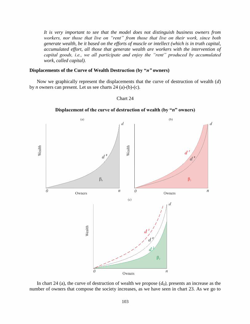
103

It is very important to see that the model does not distinguish business owners from

workers, nor those that live on “rent” from those that live on their work, since both

generate wealth, be it based on the efforts of muscle or intellect (which is in truth capital,

accumulated effort, all those that generate wealth are workers with the intervention of

capital goods, i.e., we all participate and enjoy the “rent” produced by accumulated

work, called capital).

Displacements of the Curve of Wealth Destruction (by “n” owners)

Now we graphically represent the displacements that the curve of destruction of wealth (d)

by n owners can present. Let us see charts 24 (a)-(b)-(c).

Chart 24

Displacement of the curve of destruction of wealth (by “n” owners)

In chart 24 (a), the curve of destruction of wealth we propose (d0), presents an increase as the

number of owners that compose the society increases, as we have seen in chart 23. As we go to

104

the right the number of owners and the destruction of wealth increase at the same time, i.e., we

will have more owners that destroy a greater stock of available wealth.

Figure 24 (b) shows us an upward displacement (changes in the fundamentals) of the wealth

destruction function, which indicates that d1 > d0 with the same level of n, which expresses a

greater destruction of wealth with the same quantity of owners.

Figure 24 (c) shows the opposite situation, a downward displacement of d to d2, indicating

that d2 < d0 < d1 at the same level of n, which expresses a lesser destruction of wealth with the

same number of owners.

ECONOMIC EVOLUTION OF OWNERS

Since the two curves obtained represent the behavior of subordinate variables (value of

wealth) of the same independent variable (the n owners), it is possible to combine or confront

them, the same way we did with chart 3, when we obtained the important point E, which would

then become price point EP.

Chart 25

Point R of stock

25

If we “confront” the Curve of Wealth Generation (g) with the Curve of Destruction of Wealth

(d) we can obtain an interesting chart and take advantage of the mathematical rigor we can add to

105

economics, and its consequences for explaining-analyzing human economic evolution. Let us see

chart 25.

POINT R OF AVERAGE VELOCITY OF NET POSITIVE WEALTH GENERATED,

PER CAPITA of OWNERS

In graph 25 we observe the enormous relevance of point R, which appears as the intersection of the

curve of wealth generation (g) and the curve of destruction of wealth (d). Said point, that we call point of

average speed of positive net wealth generated per capita of owners (R) –where net means generation

minus destruction, the Result in the model of double entry accounting,(46)

that is why R allows us to:

1) Express the moment, measured in terms of owners, in which the speed of generation of wealth

(slope of g) is equal to the speed of destruction of wealth (slope of d).

2) Express that: to the left of R (more specifically to the left of nR) the speed of the generation of

wealth is greater than the speed of destruction (g ˃ d), and to the right it is the opposite (g ˂ d).

3) Express the value of wealth accumulated by society at the time when the situation is that the level

of average velocity of destruction of wealth is higher than for the generation of wealth (g ˂ d).

4) Express the relation between the wealth generated by each owner and the average of all owners,

since point R indicates that while there are owners that generate wealth at a higher level than R

(where g = d), there are others that do so at a lower level. I.e., in the community of owners, there

are those that produce wealth at a level that, for society in average, it implies it is a situation

where their activity destroys more wealth than what it generates.

It is important to see the huge importance of this conclusion, above all referred to the accepted

criteria that economic activity ―specifically the study of economic cycles― is measured on the

basis of comparing the expected results with the market interest rate, which would be akin to a

“benchmark” point R, which would be inconsistent with our reasoning.

5) Express, in reference to all the preceding, the following relations that can be studied based on the

figures that arise from point R, since it allows us to relate:

a) The value of the positive net wealth generated by nR in terms of those that generate wealth at

the level where the average velocity of positive net generation of wealth is higher than the

average of destruction (g>d).

b) The value of the negative net wealth produced by the nD (= n - nR) in terms of those that

generate wealth at the level where the average velocity of the generation of positive net

wealth is lower than that of destruction (g<d).

c) The average wealth generated per capita by owners at the time when the slopes of g and d are

equated, which appears as the quotient of the value of the grey area, over nR: δ / nR.

d) With the development of the algebraic model ―system of equations and unknown

variables― pertinent for this graphic model, it is feasible to quantify the qualitative aspects

we highlight in this work.

e) In turn, through procedures of derivation and integration (total and partial) of the general

algebraic model, pertinent for the graph developed here, we can ratify the qualitative

consideration expressed in this work.

106

And other relations that are relevant at the time of judging economic policies (fiscal and

monetary), as we will have the opportunity to see.

It is worth remembering that the concepts expressed here constitute observational variables, insofar

as:

a) All the values of wealth (q*p) are expressed in the economic unit of measure, the price of

economic goods in terms of the economic good currency [pq(m)].

b) All the concepts of wealth are considered in terms of the current institutional and technical

structure in a community of n owners. I.e., stock and distribution are “data” of reality, insofar as

we are referring to stocks of economic goods multiplied by the currency prices generated in

exchanges (market) and the distribution of their property. I.e., wealth and its distribution are

economic entities that are ontologically complementary, with their pertinent observable

variables.

Finally we stress that we could observe the model with a graph that showed directly the curve g with

the destruction of wealth deducted and represented by curve d, in such a way that the new curve of

generation of net wealth (gN) would be equal to the difference g – d. In this way we would have an only

net curve of the generation of wealth (gN) ―that would cross the ordinate axis at the point R, since from

there it would become negative― based on the curve of generation of wealth (g) and the curve of the

destruction of wealth (d):

gN = g – d

The importance of handling this equation when producing algebraic developments is evident, but to

the effect of visualizing the consequences in graphic form we will continue with the scheme of the figure

of graph 25. This will be relevant when explaining the economic evolution of a society, since the

parameters for wealth generation are different for those related to its destruction (¿with the hedonism of

politicians intervening?) when speaking of society, as we shall see.

THEORETICAL CONNOTATION OF POINT R – Generation of wealth and economic

calculus theorems

We cannot continue without considering the theoretical importance of point R, since it

indicates that:

Reiterating the preceding, there always exist economic activities generating net negative

wealth, based on measuring them according to the parameters of all the generators of

wealth. This fully ratifies that all economic activities are governed by the subjective value

of the agent in consideration, therefore the parameters that appear by simple aggregation

of numbers must be considered with adequate scientific rigor, insofar as an activity can

be initiated even it does not respond to “social” parameters. The demonstration is self-

explanatory since all the wealth generated by the generators, at the right of point nR were

and are produced in those conditions.

The statement in the previous paragraph anticipates different consequences on the

number of individual owners generating wealth, which acquire and lose this condition

with changes in curves g and d, resulting from the changing conditions of their reality

107

(productive structure, economic policies, catastrophes, etc.). Consequences the quality

and quantity of which will depend on the slopes of the curves g and d.

If we consider the level of point R as the parameter based on which we will decide the

suspension of any new project of wealth generation, evidently none should be undertaken

beyond point R. But this would lead us to a point R to the left of the original, which is

establishing a new “Average” point R of all the owners, leading us to a similar situation,

and so on indefinitely ― a typical vicious circle. This allows us to express the following:

Theorem of wealth generation: all communities of human beings have producers-

activities that generate negative wealth, according to the level of average velocity of net

generation of wealth. Considering negative wealth to be that which produces less positive

net wealth than what corresponds to point R.

Though this is the law that relates al average figures with the marginal (and total) figures,

it is no less true that it has very relevant economical and political connotations when

referred to point R, since it allows us to analyze the individual based on the collective,

though we alert on the danger implied by the methodology based on “aggregates”:

1) Demystifying in this case the repeated concept of “urban legend” that humans only

act in terms of what “society” considers wealth. I.e., the theorem ratifies the theory of

subjective value.

2) There is no fallacy of composition between individual conduct and that of the whole.

This would only be explained if we forget the mathematical relation between

marginal, total and average figures. I.e., the fallacy would be of a mathematical

nature.

3) It demystifies the possibility of developing theories based on the perfect functioning

of markets, since it would imply perfectly identical supernatural humans that, when

acting would know with total precision how it would alter the level of average

velocity of net positive wealth generation (in truth, zero, because at point R: g – d =

0) of the community as a whole, and at each instant. Not forgetting in turn the

theoretical and factual impossibility, because of the vicious circle of the generation at

point R, that results as an average.

4) It disqualifies all authoritarianism that could pretend to govern the destinies of

individuals, different by nature when valuing, in terms of valuing, based on

parameters generated by averages derived from aggregates. Evidently in our case we

are referring to currency and financial policies, since according to the axioms of

equality (im = pm) and equivalence (im ≡ pm) (48)

pretending to establish and/or control

the rate of interest, implies doing so based on the price of the unit of calculus. I.e., we

do not consider in our work the entity interest, which considering the axioms of

equality and equivalence (currency-financial) implies that any action to control what

is known as currency interest, is equivalent to currency policy, with the consequences

we shall see.

We can say we have proven the correctness of the Hayekian statement referred to the

fatal arrogance.

108

5) Market currency interest rate (im): the wealth generation theorem implies said rate is

referential information for the investor, since it tells him (ceteris paribus) not to pay

more than what the resource economic time is worth in the market ―we consider

interest a the price of economic time. I.e. Said rate only operates as a cost of

opportunity (very important certainly) but it does not imply you reject an investment

if it can only be carried out with a higher financial cost than im, as long as the level of

net wealth generation of the project is higher. This reflection is not unimportant, since

all generators of wealth to the left of nR would be in that situation. On the other hand,

as we have stressed, you could not justify the existence of wealth generators to the

right of point nR.

I.e., im does not operate as an exclusive benchmark justifying the generation of

wealth. Proof of this is the wealth always generated below the levels of average net

wealth generation velocity. We have personally promoted successful projects that had

a financial cost higher than im, and helped maintain projects that “circumstantially”

operated below im.

Evidently the theorem of wealth generation solves the theoretical question of the

theory of interest and capital productivity clarifying that wealth is generated in each

economic activity, as long as its level of generation of wealth (its own g) is higher

than the level of destruction of wealth (its own d). An aspect that once again shows us

that accounting is the best model, insofar as this reflects that the company generates

positive results (operates in an area where: own g > own d, that is the same as: own g

– own d > 0, which is more than profit in accounting terms), considering in its costs

the “price of economic time”, interest, but the interest it pays, not the market average.

I.e, including in costs (destruction of wealth) the price of economic time (interest)

does not respond to a different condition from including any input, nobody would pay

more than the buying price in the market. Which ratifies the theory of interest of TET,

not meriting different treatment, since it is always represented by economic goods. (49)

6) Laffer Curve: point R can be considered in the analysis of this curve, referred to when

an increase of fiscal rates results in a reduction of tax collection. Nevertheless, our

point R is much broader, since it also includes currency policy.

7) The blessed profit: finally point R shows that any attempt to reduce, confiscate or

attack company profits or increase the destruction of wealth which is what is

promoted with the so called “welfare policies” must be reviewed, since the result is

the opposite of what their good intentions pretend.

Impossibility of calculus in collectivism: (50)

if all human beings were economically equal

in every spatiotemporal instant we value, the generation and destruction of wealth would

present a uniform behavior ―measured from the aggregate of wealth (a sphere in which

it is feasible to compare the individual and society) that they generate, which implies the

feasibility of occurrence. This would not only present parallel and horizontal g and d

curves but, what is worse, it would determine which is above or below or if they are at

the same level.

Evidently only with the model of curves g and d we are developing we can corroborate

the impossibility of calculus in collectivism, what Mises imprecisely referred to when he

said economic calculus could not be implemented in collectivism because there are no

prices. Here we have shown it is not so, but that the impossibility of economic calculus

109

would be in the only case of human beings being (economically) equal ―measured from

the aggregate of wealth (a sphere in which it is possible to compare the individual and

society) that they generate, which makes difficult the factual possibility of its occurrence

― and since this is impossible both theoretically and factually, it is impossible for

economic calculus not to exist. I.e. what does exist is the intent to alter human nature,

collectivism is theoretically and factually impossible, if as such we consider that

possibility of equality in the valuation of individuals ―two people can buy at the same

price but the reason are different always.

Therefore what we have proven is the theoretical and factual impossibility of

collectivism.

Theorem of economic calculus: given that an only individual calculates economically

and the theoretical impossibility of the existence of a community of individuals that value

economically in the same way (generate and destroy wealth at the same level all the time)

we can enunciate the following calculus theorem:

Human existence implies economic calculus

Denying economic calculus would imply denying human economic fallibility (scarcity of

goods) and the marginal laws of decreasing utility and yields, and increasing effort.

Negations in which are based the developments that necessarily must be based on the

premise of the equality of individuals.

So the theory of the model presented here allows us to conclude:

The feasibility of economic calculus does not depend on the existence of computers,

instead computers appeared and are useful for economic calculus. In other words the g

and d curves of the model show how inconsistent it is to defend the idea that communism

would have survived if computers had existed before, on the contrary, computers

appeared because of the possibility of economic calculus, without which the human

species would not have progressed (and from that progress came computers).

The indeterminacy of the subjective value, in value observable through quantities of

economic goods, is only pertinent in an imaginary world of “all equal”. On the contrary,

the human condition of “all different” is what guarantees the existence of economic

calculus.

We can theoretically deduce that institutional intervention that imply “leveling” the g

and/or d curves, imply in turn an obstacle to economic calculus. With progress in this

work we will show practically what economic institutions and policies imply not only for

the g and/or d curves, but also for point R and its implications for nR.

Having completed this necessary detour, of theoretical importance that does not end here, we

come back to our analysis ―also theoretical― of the connotations derived from the analysis of

point R.

BEHAVIOR OF THE R POINT

Now we will study the behavior of the displacement of point R (the result of the behavior of

the generation and destruction of wealth). Let us see and study charts 26 (a)-(b)-(c).

110

In chart 26 (b) we have begun the study of the behavior of point R, supposing the

displacement of g with d and n constant. Let us see the conclusions:

Chart 26

Displacement of g with d and n constant

1) In chart 26 (b) we suppose an upward displacement of g from g0 to g1, with g1 > g0 for

any n. I.e., we are in the presence of ↑ g with d and n constant, which implies:

a) An increase of δ, given taht δ10 > δ00. We observe that ↑ δ = δ10 – δ00

b) An increase of R, given that R10 > R00. We observe that ↑ R = R10 – R00.

111

c) An increase of the owners that conform the per capita wealth ↑nR, given that nR10 >

nR00.

d) In this case we conclude the resulting increase of ↑δ = δ10 – δ00, indicated in 1-a, can

be sythesized as: ↑δ = ↑g ↑n.

All which is reflected in this table:

Table 8

With d0 constant and displacement ↑g1

2) In chart 26 ( c) we suppose a downward displacement of g from g0 to g2, with g2 < g0 for

any n. I.e., we are in the presence of ↓ g, with d and n constant, which implies:

a) A decrease of δ, given δ 20 < δ00. We observe that ↓ δ = δ20 – δ00.

b) A decrease of R, given R20 < R00. We observe that ↓ R = R20 – R00.

c) A decrease of owners conforming per capita wealth ↓nR, since que nR20 < nR00.

d) In this case we conclude the resulting decrease of ↓ δ = δ20 – δ00, indicated in 2-a, can

be synthesized as: ↑δ = ↓g ↓n.

All which is reflected in this table:

Table 9

With d0 constant and displacement ↓ g2

Let us proceed now to charts 27 (a)-(b)-(c):

In chart 27 (b) we continue the study of the behavior of R supposing the displacement of d

with g and n constant. Let us see the conclusions:

3) In chart 27 (b) we suppose an upward displacement of d from d0 to d1, with d1 > d0 for

any n. I.e., we are in the presence of ↑d, with g and n constant, which implies:

a) A decrease of δ, since δ01 < δ00. We observe that ↓ δ = δ01 – δ00

.g R .n g = d ,δ Arrow R

↑ g1 R00 → R10 nR10 > nR00 (gd)10 > (gd)00 δ10 > δ00 → ↑

.g R .n g = d Δ Arrow R

↓ g2 R00 → R20 nR20 < nR00 (gd)20 < (gd)00 δ20 < δ00 ← ↓

112

b) An increase of R, since R01 > R00. We observe that ∆R = R01 – R00.

c) A decrease of owners conforming per capita wealth ↓nR, since nR01 < nR00.

d) In this case we conclude the resulting decrease of ↓ δ = δ01 – δ00, indicated in 3-a, can

be synthesized as: ↓δ = ↑d ↓n.

Chart 27

Displacement of d with g and n constant

All which is reflected in the following table:

113

Table 10

With g0 constant and displacement ↑ d1

4) In chart 27 (c) we suppose a downward displacement of d from d0 to d2, with d2 < d0 for

any n. I.e., we are in the presence of ↓ d, with g and n constant, which implies:

a) An increase of δ, since δ02 > δ00. We observe that ↑ δ = δ02 – δ00.

b) A decrease of R, since R02 < R00. We observe that ↓ R = R02 – R00.

c) An increase of the owners that conform per capita wealth ↑nR, since nR02 > nR00.

d) In this case we conclude that the resulting increase of ↑ δ = δ02 – δ00, indicated in 4-a,

can be synthesized as: ↑δ = ↓d ↑n.

All which is reflected in the following table:

Table 11

With g0 constant and displacement ↓ d2

CURVE OF THE ECONOMIC EVOLUTION OF OWNERS (CEE-O)

We are ready to study the behavior of the economic evolution of n owners, which we will do

with chart 28 that we analyze now.

In chart 28 we show the extreme cases presented previously, upward and downward

displacement of the curves of Generation (g) and Destruction (d) of wealth by n owners. So we

concentrate on the R points resulting from the intersections g and d: R00 of the intersection g0 ↔

d0; R11 of the intersection g1 ↔ d1; R21 of the intersection g2 ↔ d1; R22 of the intersection g2 ↔

d2, y R12 of the intersection g1 ↔ d2. In turn, each one with the related coordinate point g = d, y

nxx.

The study is carried out drawing the curve of economic evolution (CEE), which will consist

of linking the points Rxx, from the point of origin R00 to the arrival point, and in the same order

the relation of the coordinates that determine each one of them (gxx = dxx y nxx).

Now we will analyze the consequences of the displacements of the curves of Generation (g)

and Destruction (d) of wealth that can occur ―according to the implicit cases in the figures used

here―, and their consequences in the movement of the curve of economic evolution of the

owners we will present. The reader can do the pertinent analysis of movements within the

curves, combined with displacements. On the other hand, it is possible to study the inverse

.d R .n g = d Δ Arrow R

↑ d1 R00 → R01 nR01 < nR00 (gd)01 < (gd)00 δ01 < δ00 ← ↑

.d R .n g = d ,δ Flecha R

↓ d2 R00 → R02 nR02 > nR00 (gd)02 < (gd)00 δ02 > δ00 → ↑

114

behavior to those shown here, supposing simply the final positions are the origins and the origins

are the final positions.

We analyze first the behavior of Rxx referred to its incidence on the equation gxx = dxx, with

the displacements of the curves.

Chart 28

Curve of Economic Evolution of “n” owners

Based on chart 29 we analyze the three cases we wish to distinguish, using the horizontal

shaded band surrounding the level of R00, to visualize the consequences of the displacements of g

and d on the level of R, let us see:

a) Rise of the level of R above the shaded band, where we only observe R11, produced by

the upward displacement of the curve of generation of wealth (↑ g1) and the upward

displacement of the curve of wealth destruction (↑ d1): R00 → R11.

115

b) Fall of the level of R, below the shaded band, where we only observe R22, produced by

the downward displacement of the wealth generation curve (↓ g2), and the downward

displacement of the curve of wealth destruction (↓ d2): R00 → R22.

c) Approximate similarity of the level of R, above the shaded band, where we observe R12

and R21, because the effects of an upward displacement of the wealth generation curve

(↑g1) are neutralized by a downward displacement of the curve of wealth destruction (↓

d2): R00 → R12; and a downward displacement of the wealth generation curve (↓ g2) with

un upward displacement of the curve of wealth destruction (↑ d1): R00 → R21.

Chart 29

Behavior of R with displacements of the curves g and d

We stress that similar displacements of g and d that do not neutralize each other, they present

more profound variations in the behavior of R. This is different from the opposing movements of

g and d, where the upward displacement of one is “compensated” with the downward movement

of the other, producing smaller oscillations in the behavior of R.

116

Now we will analyze the behavior of the number of owners participating in the formation of

average per capita wealth (nxx), i.e., what the behavior of the distribution of wealth indicates with

displacements of the curves of generation and destruction of wealth. Let us see and analyze chart

30.

Chart 30

Behavior of nxx with displacements of curves g and d

Based on chart 30 we analyze the three cases we wish to differentiate, using to this effect the

shaded vertical band surrounding the level of R00, to visualize the consequences that the

displacements of g and d have for nRxx.

a) Rise of the level of owners nR, to the right of the shaded band, where we only observe

nR12, due to an upward displacement of the wealth generation curve (↑g1), with a

downward displacement of the curve of wealth destruction (↓ d2): R00 → R12.

117

b) Fall of the level of owners nR, to the left of the shaded band, where we only observe nR21,

due to a downward displacement of the curve of wealth generation (↓ g2), with an upward

displacement of the wealth destruction curve (↑ d1): R00 → R21.

c) Approximate similarity of the level of owners nR, included in the shaded band, where we

observe nR11 (beside nR00), originated in the upward displacement of the wealth

generation curve (↑ g1) with an upward displacement of the wealth destruction curve (↑

d1): R00 → R11; and R22, originated in the downward displacement of the wealth

generation curve (↓ g2), with a downward displacement of the wealth destruction curve (↓

d2): R00 → R22.

We observe a behavior that is different from R, since here there are larger oscillations in n

following a different behavior of g and d.

It is evident that the completely different consequences in the behavior of R and n, with the

same combined behavior of g and d, will be very useful for economic analysis. Analysis we will

now develop and that surely will not exhaust the analytical field open here.

Now we eliminated the shaded area and concentrate on the combined effects on R and n of

the proposed displacements of g and d. Let us see the following chart 31.

In chart 31 we observe that:

a) A higher level of per capita wealth, concentrated in a similar number of owners: R11 y

nR11, originated by the upward displacement of the curve of wealth generation (↑ g1),

with an upward displacement of the wealth destruction curve (↑ d1).

b) Lower level of per capita wealth, concentrated in a similar number of owners: R22 and

nR22, originated by the downward displacement of the curve of wealth generation (↓ g2),

with a downward displacement of the wealth destruction curve (↓ d2).

c) Similar level of per capita wealth, concentrated in a smaller number of owners R21 and

nR21, due to a downward displacement of the wealth generation curve (↓ g2), with an

upward displacement of the wealth destruction curve (↑ d1).

d) Similar level of per capita wealth, concentrated in a greater number of owners: R12 and

nR12, due to an upward displacement of the wealth generation curve (↑g1), with a

downward displacement of the curve of wealth destruction (↓ d2).

Finally, in chart 31 we clearly observe the difference between the areas that represent the net

wealth generated between the two extreme cases limited by R21 (with black frame) and R12

(shaded).

Now we simplify the data and present chart 32 in which we only highlight the R points

generated at the ends of the displace curves (R21 y Rl2).

We should not forget that the analysis of this section refers to comparing the new extreme

positions (R21 y Rl2). Derived from the also extreme curves of wealth generation and destruction

(g2d1 y g1d2), relative to an original position R00, derived from g0d0 from where we start the

comparative analysis.

118

Now let us see what analysis we have when we compare directly two positions we are

interested in analyzing, i.e., we do without the original position (R00) ―that we use as a

mediation for expositive reasons and to show a non linear process― and directly compare two

positions that will be necessarily different.

Chart 31

Combined consequences for R and n of displacements in g and d

To this end we present chart 32 where we directly show the “movement” between R21 ↔ R12,

representative of the real cases that we can compare in a world in constant change, i.e., where

none of the curves remain constant and we analyze specific data taken from reality. Let us see:

We could say the curve of economic evolution of “n” owners (CEE-O), represented by the

line with an arrow at both ends is the behavior of the economic evolution of a community, since

we have represented the extreme wealth generation and destruction curves, with the clear goal of

making a synthesis of the trend a CEE-O should present. We observe that:

119

R21 → R12: as the number of owners increases (nR21 → nR12), in a situation where

wealth increases (g2 → g1), and its destruction decreases (d1 → d2), there is a

considerable increase in the distribution of wealth, with distribution among many more

owners, with a moderately higher at a level of average speed of positive net wealth (R21 y

R12 were in the shaded band).

Chart 32

Curve of Economic Evolution of Owners (CEE-O)

R21 ← R12: as the number of owners decreases (nR12 → nR21), in a situation where

wealth decreases (g2 ← g1), and its destruction increases (d1 ← d2), there is a

considerable decrease in the distribution of wealth, with distribution among much fewer

owners, with a moderately lower at a level of average speed of positive net wealth (R12 y

R21 were in the shaded band).

120

In turn, the synthesis of the human correlation of quality and quantity is reflected in the

CEE-O with the relation R21 ↔ R12, while we observe that R21 > R12 shows us:

1) The presence of the law of diminishing returns: since as the number of owners expands,

the level of velocity of net generation of wealth decreases: to nR12 > nR21 corresponds R12

< R21, and vice versa: to nR21 < nR12 corresponds R21 > R12. Which is indicating that the

expansion of wealth happens at the expense of a lesser level of individual intensity of

wealth (as in physics, chemistry, economics, etc.). This is what we observe in the

business world: they are born in a niche with few users at a high price, then they go

through the process of differentiation with middle quantities and prices and through

competition end up with low prices for a great number of users.

2) The relationship (R21 ↔ R12), synthesis of the inter-play of the behavior of the slopes of

the curves of wealth generation and destruction, would validate the ideas of many

scientists, especially in the field of physics, that the more we know the more ignorance

we see. I.e., as humans increase their wealth, they discover the infinite that can be

generated is wider and more complex ―both in the micro and the macro― a situation

that the previous state of relative poverty did not allow us to appreciate. The business

world works in the same way, insofar as competition tends permanently toward greater

wealth, except when institutions discourage this, in which case there is an involution to

previous states of poverty.

3) If we consider the downward slope of the wealth generation curve relative to the passing

of time, we can conclude that all stock of wealth (value) can be considered “non

renewable”, since we know that as time passes it presents “different forms”. This

categorical conclusion determines that non-renewable natural resources should not be

considered a special or strange case, since the same will be true for all wealth.

4) These reflections ratify that the fallibility of human beings implies the condition of

maximizer by nature. I.e., it would not be conceivable to analyze man outside this

condition of maximizer, insofar as this is determined by the nature present in human

action (Popper and Mises) and the marginal laws. Humans try to maximize the stock of

wealth, knowing they will never reach the maximum possible.

We can summarize the behavior of the curve of economic evolution, saying that any

expansion of wealth among individuals (increase of n) implies supposing that is achieved

with a lower level of R. A situation than can only change if the progress in g

overcompensates the increase in the concomitant destruction presented by the progress of d.

The most favorable answer will always be in economic education, leading to institutions that

do not alter the free functioning of the marginal laws and allow ―it is not necessary to

promote― the maximization of individual and collective efficiency.

Finally, it is important to stress that the process of the economic evolution of “n” owners

does not present a linear relation as we have seen in chart 32, instead it is more appropriate to

think of it as a “spider-web” figure, with the help of the theoretical understanding derived from

chart 32, and of reference point R00.

121

DISPLACEMENT OF CEE-O FROM A SPATIO-TEMPORAL POINT

We must stress that the conclusions we have reached derive from the institutional framework

existing in society that determine the levels of the slopes of the curves of wealth generation and

destruction and their displacements. All of which allows us to conclude in chart 33, and thus

summarize the model and present the economic evolution of “n” owners as a non linear

whirlwind that moves towards one of the quadrants we can consider once we have established

the center of the axis of coordinates in a point R00. Which would be the equivalent of analyzing

the behavior of the Curve of Economic Evolution of Owners starting from a certain spatio-

temporal point.

Chart 33

CEE-O from a spatio-temporal point

Chart 33 (cross) ―the fact that this coincides with the number 33, the age of Christ on the

cross, is pure chance― must be interpreted with the fundamentals of the CEE-O, only we have

122

placed the center of coordinates at a point R00. An exercise that allows us to study the possible

derivations of the CEE-O of each concrete case, as long as there is the adoption of policies for

changing the institutional structures underlying the behavior of the curves of generation (g) and

destruction (d) of wealth, with corresponding framework of distribution among owners of the

same. In other words, it would be like drawing on the charts we have presented an infinity of

temporary CEE-O starting from an initial spatio-temporal point. From another perspective, any

CEE-O is a synthesis of infinitesimal and continuous curves derived from the immediately

preceding spatio-temporal point, where the crossing of the original ordinates would be the

beginning of the economic evolution of the owners under study.

Chart 33 shows us:

Two horizontal sections: the one corresponding to the behavior of the level of generation

of net wealth (R) showing an increase (↑ Rxx) above the abscissa, and a decrease (↓ Rxx)

below it.

Two vertical sections: indicating the exclusion of individuals (↓n) that participate in the

generation of net wealth, to the left of the ordinate, and inclusion (↑n) to the right.

With the help of chart 33 we can predict synthetically the possible scenarios of economic

evolution, starting from a spatio-temporal point of diagnosis (R00) and evaluate the path with

highest probability, which will be circumscribed to one of the referred quadrants.

Quadrant 1: Increase of the level of net wealth generation with exclusion of owners.

Quadrant 2: Increase of the level of net wealth generation with inclusion of owners.

Quadrant 3: Decrease of the level of net wealth generation with exclusion of owners.

Quadrant 4: Decrease of the level of net wealth generation with inclusion of owners.

The possibility of the occurrence of any of the four phenomenon puts us in a terrain where

we cannot speak of a virtuous path of economic growth of owners with an axiomatic spirit. I.e.,

there is no dogma that stipulates a positive correlation between the economic evolution of the

owner and the society to which he belongs, but there is a specific way to reach one or the other

goal, which refers to allowing the free functioning of the marginal laws.

Chart 33 clearly indicates that the evolution of the individual and society are not always

positively correlated, and that it is prudent to choose rationally the best method according to the

goal of society, based on a point of diagnosis. Even so, it is clear there is only one way to reach

the economic goal, the benefit of demand, and that is allowing the full functioning of the

marginal laws.

Conclusion: we can ratify that all societies have much to say when explaining their poverty

or wealth, a situation that becomes exponential as we follow the a priori logical-deductive

causality of economics, and include in the analysis the individuals of the community that are not

123

owners, do not participate in the generation of wealth but do intervene in this destruction, with

which we will have completed the study of Socio-Economic Evolution.

We must also remember the consequences we studied when analyzing chart 32, where we

compared the consequences derived from the extreme positions of the curves of generation (g)

and destruction (d) of wealth. There we concluded that the consequences of the displacements of

the curves were more devastating off the distribution of wealth than for the average level of

wealth, corroborated by post crisis statistics. Which should be an alert when establishing

“economic policies”.

To confirm all this what follows will be necessary and sufficient proof reflecting which

policies that have been applied (fiscal, currency-financial, employment, etc.) have originated

displacements towards one or the other quadrant of the curve of socio-economic evolution

starting from a specific spatio-temporal point.

124

SOCIO-ECONOMIC EVOLUTION

Endogenous institutions and economic policies

In this section we add to the a priori logical-deductive causality of economic evolution

another component of the reality of a society, the economic support of individuals that are not

economically active ―only destroy wealth―, which we will designate as nD.

It is of great importance to see this inclusion implies considering economic policy (currency

and fiscal) as an endogenous variable of the model we are developing ―a theoretical framework

suggested by Milton Friedman for future developments, recognizing the lack thereof up to that

moment.

To do this it is very useful to resort again to the CEE-O we have developed and so we obtain

chart 34.

Chart 34

Curve of Socio-Economic Evolution (CSEE)

125

In chart 34 we have added more individuals to the n set that represented the labor force

(which from now on we will designate as nO, where the subscript O denotes the condition of

owner). Thus we extend the abscissa to represent the total population (nT), from where we

deduce that the part of the population that is not part of the labor force (nD) is the difference

between the two others:

nD = nT – nO

In chart 34 we highlight the consequences of including nD insofar as they do not generate

wealth but do destroy it:

We extend the abscissa to the effect of adding the individuals that are not part of the labor

force (nD) that compose society. In this manner we have the quantity of owners from the

origin (0) to nO, and from nO to nT the individuals that are not owners or are not part of

the labor force nD, since they do not generate wealth. We have already stressed the fact of considering humans that generate wealth in the abscissa (np)

that, being ordered based on the law of decreasing yields, implies considering the distribution of

wealth according to the owners that generate it. Now we include the humans that participate in

the destruction of wealth generated by them that do so based on the institutional political order

with which they are introduced to the economic world. I.e., here we complete the framework of

wealth distribution, since we add those that are benefited with participating in the destruction of

wealth that they do not generate.

We reiterate a previous statement:

…the generation of wealth obeys an aspect governed by economic laws (crudely

mentioned as market laws), while the destruction of wealth is governed by political

factors ―here is the endogenous treatment of economic institutions and policies.

We start from g, since it is the curve of wealth that generates nO.

We start from dO, since it is the curve of destruction of wealth by nO.

We start from RO, since it is point R for the described curves that present the equation g =

dO, for nO.

The curve of total wealth destruction, that adds nD, is represented by dT.

The new point RT appears as the intersection of g = dT.

The surface of wealth destruction βT (framed in red) appears representing the stock of

wealth destroyed with nT. For comparison we frame βO in green, representative of the

destruction of wealth for nO, before including nD.

The surface δnT is formed, representing the surface of net wealth generated by g and dT,

not represented in this chart, which is defined by 0; g; g; RT; nRT. For comparison we

highlight δnO, that represents the surface of net wealth generated by g and dO also not

represented in this chart, defined by 0, g, g, RO, nRO.

126

The red arrows, by the coordinates, show the behavior of the variables represented in

them: increase of nD individuals in the abscissa (nO → nT), decrease of owners

participating of the minor net wealth in the abscissa (nRT ← nRO), and increase of new

point R, indicated in the ordinate (gdO ↑ gdT).

Endogenous economic policies: here we reiterate the enormous importance of having

confronted the g curve of generation of wealth ―decreasing from its origin (according to

market terms)― with the d curve of wealth destruction increasing from its origin,

according to political terms. I.e. we can clearly see the huge importance of presenting the

d curve that ascends with the increase in the number of individuals, as we stressed in its

first construction, in which we only referred to the wealth destroyed by the owners.

We end this section refreshing an aspect that is essential to understanding how the g and

d curves relate: while curve g represents the wealth generated in a period of time, the d

curve represents the wealth destroyed in that same period of time, “but” includes also the

pre-existing wealth that is destroyed in the period. In other words, while in a period only

“new” wealth can be generated (represented by the g curve), the d curve refers to the

destruction of wealth in the period, which implies the possibility of destroying “new” and

pre-existent wealth.

Let us see the consequences of including human beings that only destroy wealth:

Table 12

Behavior of Socio-Economic Evolution (CSEE)

It is not strange that we are in the presence of the same consequences as when we studied the

increase in destruction of wealth (table 10). A cursory examination will show:

Table 13

With g constant and displacement ↑ d1

Then all the conclusions we reached when studying the consequences of bigger curve of

wealth destruction are valid for the transition from nO to nT, due to the inclusion of nD.

dT R .n g = d ,δ Arrow R

↑ dT RO < RT nRT < nRO (gd)T > (gd)O δT < δO ← ↑

d R .n g = d ,δ Arrow

↑ d1 RO < RT nRT < nRO (gd)T < (gd)O δT < δO ← ↑

127

Finally we stress the new forms of the areas deriving from chart 34 (not drawn):

δT < δO

Which also allows us to say that with the difference δT - δO we can evaluate the effort of a

community to sustain nD, from the analysis of the net wealth generated, in terms of economic

goods, weighted by their prices relative to the currency.

From another point of view:

βT > βO

It allows us to say that with the difference βT - βO we can evaluate the effort of a community

to sustain nD, based on the analysis of destruction of wealth, in terms of economic goods

weighted by their prices relative to the currency.

Thus we can deduce:

δT - δO = βT - βO

It is the same if we take δ or β, it is clear that the marginal laws of diminishing utility and

returns establish that anything that implies promoting destruction of wealth, that is, promoting

consumption, is negative for social economic evolution. In this way productive efficiency once

again becomes man’s best ally. Among the manifestations of efficiency we highlight simplicity

(one of the requisites of Popper to prove a theory is superior to another) which in economics

implies “no bureaucracy” in the Misian sense.

128

PART III

PROPOSED

MACROECONOMIC

MODEL

― APPLIED ―

129

CURRENCY AND FISCAL POLICY

We will now consider what is called:

1) Fiscal policy: considering as such imposing on the owners (nO) covering the cost of the

destruction of wealth by non-owners (nD).

2) Currency policy: considering as such the control of bank currency and credit, with which

there is the pretense of controlling alternatively the general level of prices (which for us

is the price of currency) and/or the currency interest rate (not considering the validity of

the equivalence axiom presented by TET: im ≡ pm). All this with the intention of

controlling what they call the “general” level of prices (inflation) and the level of

unemployment, which they try to explain with the IS/LM models, the Phillips curve and

its different interpretations, etc. Within the framework of the axioms of equality (pm = im)

and equivalence (pm ≡ im) of TET, it is evident that currency and financial policies are

mutually implied.

What we have considered as fiscal policy is represented by our socio economic evolution

curve, since we have already added the incidence of the passage from nO to nT, adding the non-

economic members of a society, nD. We must reiterate that nD includes the members of society

that are non-economic, non-owners, that do not generate wealth and are not supported by direct

family or solidarity ties with an owner. In other words, the members of a family are included in

nO and anyone that receives subsidies belongs to nD. (51)

To this effect we now draw and analyze chart 35.

In chart 35 we highlight the consequences of including simultaneously fiscal and currency

policies. Let us see the components:

Compared with previous charts, we have only replaced the subscript T (Total) with the

subscript F (Fiscal), representative of the concept that those that generate wealth must

now support the whole population with taxes (fiscal policy).

Fiscal policy is represented by the inclusion of nD, expressing the distance between nO

and nF, which we have already seen, which generates the curves dF and dO we already

know, determining the points RF and RO, we also know.

On the chart of the three curves representative of socio economic evolution that we

already had (g, dO, dT=F) we have drawn in red the three new curves that appear with a

currency expansion (↑M) that causes a fall of the price of currency, unit of measure with

which we weight when valuing the generation and destruction of wealth.

We start from g, that is the curve of wealth generated by nO.

We start from dPO, that is the curve of wealth destruction by nO.

We start from dF, that is the curve of wealth destruction by nF.

We start from RF, that is point R for the curves g and dF.

We start from RPO, that is point R for the curves g and dO.

Ceteris paribus: ↑ M implies ↓ Pm(q), ↓ Pm, o ↓ pm.

We build gM

, that is the curve of wealth generated by nM

P with ↓ pm for ↑M.

130

We build dM

PO, that is the curve of destruction of wealth generated by nO with ↓ pm for

↑M.

We build dM

F, that is the curve of destruction of wealth generated by nF with ↓ pm for ↑M.

Chart 35

Curve of fiscal and currency policy combined

We build RM

F, that is point R for the curves gM

and dM

F with ↓ pm for ↑M.

We build RM

O, that is point R for the curves gM

and dM

O with ↓ pm for ↑M.

Let us see the consequences of fiscal (F) and currency (M) policy separately and together:

Since we have already studied fiscal policy when we analyzed nD ―the inclusion of the

support of non-owner individuals by owners (the reason for their being taxes), a situation that

existed before currency (there is fiscal policy without currency policy) ― now we concentrate on

131

the analysis of adding currency policy to a state with a pre-existent fiscal policy. So let us

analyze the consequences of a currency policy added to a previous fiscal policy:

Table 14

Analysis of fiscal and currency policy

Policy g .d R .n ,δ β Arrow

R

F dF >dO RF > RO nF > nO δF < δO βF > βO ←↑

FM gM

< g

dM

F < dF RM

F < RF nM

P < nO δM

F < δF βM

F > βF ←↓

Generation of wealth (g): the fall of the price of currency produces a decrease of the

value of wealth with the same currency used for calculus. The inexistence of any

currency “veil” is ratified, insofar as our human action is guided by the quantity-price-

currency, which is always “real” in a world with currency.

Destruction of wealth (d): the fall of the price of currency produces a decrease of the

value of the destruction of wealth with the same currency used for calculus. Again the

inexistence of any currency “veil” is ratified.

Unemployment (← nO): reflected in a lower level of owners indicated by nM

O < nO, which

does not surprise us in the CEE since we are in the presence of net wealth destruction,

which is generated with the fall of nO: less wealth is produced by less owners (ceteris

paribus). The same situation of distributive involution is presented by nDM > nD.

Result (R): the fall of the price of currency results in:

1) The velocity of per capita average net wealth generated is valued less: (RM

F < RF) o

(↓R). The inexistence of any currency “veil” is ratified.

2) The deterioration of the wealth distribution, i.e., once again the reduction of wealth

implies worse distribution of the same (← n).

3) The deterioration of the effort of n owners supporting the fiscal policy as long as the

quantity of individuals (nF) is not altered, but the number of owners is reduced (which

is observed with nM

O < nO and nDM > nD), which in turn will lead these to elude fiscal

policies, generating a vicious circle.

Before we go on to a graphic representation, which will allow us a simpler understanding of

the consequences of the implementation of fiscal and currency policies, it is necessary to

reiterate that: while the first produces a displacement of point R within the same g curve

―regressive distribution of wealth: RF ˃ RO and RM

F ˃ RM

O ―, the second produces a

displacement of the g curve (and the d curve) ―generalized regression of wealth, generation and

132

destruction: gM

˂ g y dM

˂ d)―, where the new R points are established. Which demystifies the

belief that currency policy has the same consequences as fiscal policy; both have an effect, but in

different ways.

The advanced reader of economic theory will see some theoretical consequences of

enormous importance compared to developments of the twentieth century destined to explain

what we explain here. The reader will see the difference with the known models, in the variables

used for the analysis of the consequences of fiscal and currency policies, which will inevitably

lead to different explanations.

Model with reduced graph

Now we will show another graph in which the conclusions regarding the consequences of

fiscal and currency policies in the economy of a society can be observed from a different

explanatory perspective that we believe to be more concise and simpler. To that effect we will

present graphs that are partial reproduction of graph 35, i.e., the parts presented are a “graphic”

copy (dimensions of the figures) of said graph, with explanatory geometrical additions.

In general terms, these graphs will allow us to see with greater clarity how the g curve slope

(and the d curve, implicit in the R points) plays in fiscal and currency policies. This graph allows

us to compare the model proposed here with known developments when studying the generation,

destruction, and distribution of wealth, and unemployment.

Before starting, we wish to point out we have introduced some changes in the terminology,

this is done to include the idea that the total population (nT) is equivalent to the “Fiscal”

population (nF) we have seen and equalize the subscripts in the ordinate, abscissa, and points R.

Fiscal policy

First we present graph 35 F, in which we refer exclusively to the analysis of the

consequences of Fiscal policy.

As we observe in the ordinate, the “transcendental” change we have introduced is

considering that the total original population nT is now in the position occupied before by nP

―the point of insertion of the g curve in the abscissa―, and that is why: 1) we exclude from our

analysis the dotted part of the abscissa, which goes to the previous nT (surrounded by dotted red),

and 2) we call the new point nF

T, with which we mean to say it is the point in which we have the

number of individuals (n) included in the Fiscal policy, equivalent to the Total population.

Nevertheless, the simplest way to include the new graphs is considering the same were drawn

starting from the range of the ordinate, i.e., the g curve (and the implicit d curve, from where the

R points appear) was built with the new structure: the g curve includes the nD, and we would

have two d curves, that also include the nD, and all of them would conclude in that new point on

the abscissa nF

T.

We begin from curve g where we represented the consequences of fiscal policy, with no

presence of currency policy.

If we draw the tangent (green) to curve g, at the point Ro, where there was no fiscal (or

currency) policy, the curve allows us to determine on the abscissa the number of owners that

generate (and destroy) wealth, which places us at point no that allows us to determine the

quantity of nD = nF

T - nO, which is equivalent to nD in graph 35. This is so insofar as the tangent

to the “new” curve g, at the “new” point RO (a consequence also of the “new” Curve d, not

133

drawn), shows us the same quantity of nO, nD and nT of the previous graph. I.e., in graph 35 we

do not need the tangent to determine the distribution of total inhabitants between nO and nD, but

now we do need it, since those values are “diluted” in the construction of the “new” curves.

Chart 35 F

Consequences of Fiscal policy

If we draw the tangent (red) to the curve g, at point RF, where there is fiscal policy (but no

currency policy), the same allows us to determine on the abscissa the new number of owners that

generate (and destroy) wealth, which places us at point nO

F, which indicates that nO

F ˂ nO, which

determines a quantity nD = nF

T - nO

F, which is equal to nD in graph 35 –because of the criterion

for building the “new” curves we have already mentioned.

So the graph clearly shows that fiscal policy implies a displacement in curve g (ascending

arrow F to the left on the same g curve), and a regressive displacement in the quantity of owners,

which will be added to the nD that originated the fiscal policy, i.e., they will increase

unemployment according to the difference nO

- nO

F.

134

It is easy to see an inverse movement of fiscal policy, a decrease of destruction by the nD,

implying an inverse displacement from point R within the same g curve, and on the abscissa

indicating unemployment.

Currency policy

Now we will show graph 35 M, where we include currency policy, which we represent in

red, different from the exclusively fiscal policy of the previous graph, that we here reproduce in

black.

So the graph adds the curve gM

of the original graph 35, which was the representation of the

inclusion of currency policy on curves g and d, not drawn here since we are interested in the

analysis of point R and the consequences for n.

First we stress we have developed the same procedure as in the preceding graph, which can

be seen observing the dotted part in red of the abscissa that would explain the function of curve g

(and curves d not drawn, but present through points R) drawn relative to the total population. In

other words, nM

T represents the total population in this drawing of curve gM

with currency policy.

We already know the main consequence of currency policy, a displacement of curves g and d

(a displacement that we know to be downward).

If we draw the tangent to the curve gM

at point ROM, representing the level for the curve gM

,

where we only have currency policy ―it is its equivalent to point RO of curve g without fiscal or

currency policy―, we determine on the abscissa the number of owners that generate wealth at

point nO

M. Point that shows the consequences of currency policy without fiscal policy, on

unemployment: nO

M ˂ nM

T ˂ nO

F ˂ nO ˂ n

FT.

But it is very important also to see that the descending displacement of curve g, to curve gM

,

originates ROM ˂ RO.

Now we add fiscal policy to currency policy, which takes us to the following analysis: if we

draw curve gM

at point RFM, representing the level of the curve gM

, where currency fiscal policy

are present ―its equivalent to point RF of curve g with fiscal policy and without currency

policy―, we determine on the abscissa the new number of owners that generate wealth at point

nO

FM. Point that shows the consequences of currency policy combined with fiscal policy on

unemployment, which is included on the succession of previous unevenness: nO

FM ˂ nO

M ˂ nM

T ˂

nO

F ˂ nO ˂ n

FT.

Again, it is also very important to see that the descending displacement of curve g to curve

gM

originates RFM ˂ RF.

Again, also, it is very important to see the downward displacement of curve g to the curve gM

originates RFM ˂ RF.

Thus, the descending displacements of curves g and d (implicit in points R) as a consequence

of currency policies (expansive that generate a fall in the price of the unit of economic calculus)

are shown with the descending red arrows indicated with M. Arrows that in turn are displaced

from right to left in both cases.

135

Chart 35 M

Consecuences of Monetary policy

Summary of the consequences of fiscal and currency policies:

Fiscal policy implies:

1) Displacements in the g curve ―remember this is produced by a displacement of curve d,

i.e., fiscal policy displaces curve d up, and produces upward displacements of point R,

within the same g curve.

2) Displacement of point R with the same curve g, because of fiscal policy, implying

upward movement of point R, with the same g curve ―with or without currency policy, g

or gM

. Then, since this derives due to the law of decreasing yields, the higher level of

point R implies higher level of the velocity of net positive wealth generation of the set of

136

producers, which is attained with a lower number of wealth generators, i.e. it implies an

increase of unemployment (∆nD).

Currency policy implies:

1) Displacement of curve g ―remember there is also displacement of curve d, i.e., currency

policy displaces both g and d, and it does so in both cases descending.

2) The displacement of curve g due to currency policy always implies the descent of point

R, both in the case of there being or not being (improbable case) fiscal policy. This

explains why currency policy is devastating, since it implies destroying “everybody’s”

wealth (no), and at the same time it does not solve the problem of the few (nD).

It is evident that the slopes of curves g and d are what will allow the evaluation of the levels

of destruction of wealth and employment generated by currency policies, but a look at the

graph by itself shows that the area of generated wealth and the point where we represent the

total population in each case had to be very restricted, which shows clearly how devastating

currency policies are when currency expansions result in the fall of the quantity-price-

currency.

We Argentines have lamentable and devastating experiences: when the monster shows its

face in the form of “devaluation”, you have the symptoms of a neutronic bomb, the buildings

are still there but the population totally sinks into destruction. Destruction that appears as a

“deepening and expansion of poverty”, as a consequence of the multiplication of the poor

(poorer than before, points RFM and ROM far below RF and RO), and on the other hand

concentration of wealth with less rich (fall of nO). A scenario of violence similar to the phase

of primitive man ―individual progress resulted from sacking the neighbor― a consequence

of leaders that take advantage of the electorate’s ignorance. Which shows arrogance is a

disagreeable personal trait, but when it refers to those who hold power and is accompanied

by ignorance, it has devastating consequences.

In short, the marginal laws of decreasing yields and marginal utility are expressed in both

fiscal and currency policies, but they appear more aggressively in currency policies. All this as a

result of the fact that all “economic policies” imply orienting the economy in search of a higher

level of point R ―velocity of generation positive net wealth of the community as a whole―

which implies an inevitable regression to a previous phase of production, with a lower level of

individuals generating wealth, and an increase in the number of individuals that only destroy

wealth.

On the other hand, those displaced of the group of generators of wealth belong to the lowest

level of productive capacity, the weakest marginal producers, because it is the place where there

is the earliest perception that effort is not valued by the community. In other words, the lowest

value is found at the end of the g curve, the first to be displaced by fiscal and currency policies

―i.e., the poor directly above pay the consequences for the poor directly below, while the

highest levels of wealth generation read about it in the papers.

137

Conclusion:

The two marginal laws of economics not only govern the relation between man and

economic goods, but also the economic relations of men among themselves. Which

implies they are sufficient and necessary for explaining human economics: wealth

(generation-destruction-distribution) and unemployment.

The model was produced considering wealth is generated in a period based on the pre-

existing productive and institutional structures, and is destroyed ―the wealth available

in the period, be it from the initial stock or that generated in the period― according to

the current economic institutions and policies. All of which not only relates the past and

to the present, but considers the economic institutions and policies as endogenous

variables of the model.

All we have expressed is captured by double entry accounting, insofar as the information,

though a-temporal, is homogeneous being expressed in the unit of measure in a specific

spatio-temporal moment, as we shall see in the practical proposal for implementation of

the model.

In this work we have corroborated another hypothesis of TET, that referred to the

economic cycles originated in currency explained by price controls, which we have

corroborated here when studying the consequences of currency policy, be it with the

intention of controlling im and/or pm (by the axioms of equality and equivalence).(52)

We consider that the methodology used in TWU and its SEE model will clarify things for

theoreticians that, confusedly in our criterion, pretend to explain economic behavior in

time with the expedient of separating the flows of consumption and rent, the relation

between present and future wealth (income), an attempt at explaining whether income

comes from wealth or vice versa.

Evidently our model does not present this contradiction since we consider the wealth

“incorporated” in the period (g) and that which is destroyed in the period, which comes

from that “obtained” in the period and from previous periods.

In short, we believe the error was in pretending to explain economic policies with the

same laws that govern the economy. Ergo, it was not possible to obtain a theory that

would explain both scenarios based on the laws that govern the economy.

The only way economic policy can be considered endogenous is considering its laws, and

thus creating a model that simultaneously contemplates the functioning of both

scenarios: the one governed by economic laws, and the one governed by political laws,

which is precisely the synthesis attained with TWU and its SEE model.

138

SOCIO ECONOMIC EVOLUTION IN HISTORY

We consider this is a good moment to introduce a brief graphic summary of all we have

deduced up to this point, with the a priori logical-deductive causality chain that we have called

theory of socio economic evolution. And it is very useful to present the evolution of human

economy through history with it. Let us see chart 36, divided in charts 36 (a) and 36 (b) for

visual reason, and that we reproduce on a higher scale as Appendix A:

Chart 36

Curve of socio economic evolution in history

Chart 36 has the following characteristics in its construction:

A social economy with nF individuals is analyzed, i.e., with a fiscal policy (nF) in a

constant population, with individuals that are not part of the labor force subsidized by

the owners.

Curves of wealth generation, g:

Red (g0): economy with currency and credit.

Green (g1): economy with currency, credit and expansive currency policy (↓ pm).

Black (g2): economy with currency, credit, expansive currency policy (↓ pm), and

decrease of credit.

Blue (g3): barter.

139

Curves of destruction of wealth dO and dF

Red (d0

F and d0

O): economy with currency, credit and fiscal policy.

Green (d1

F and d1

O): economy with currency, credit and expansive currency policy (↓ pm),

with fiscal policy.

Black (d2

F and d

2O): economy with currency, credit, expansive currency policy (↓ pm),

decrease of credit and fiscal policy.

Blue (d3

F and d3

O): barter with fiscal policy.

The displacements of point R (crosses of g with dO and dF) are defined.

The displacements of nF for each point R are defined.

The movements of the variables represented in them (gd and nF) are indicated with

arrows by the ordinates.

From chart 36 the following conclusions can be derived:

Curve of generation of wealth g:

a) Economic involution:

140

g0 > g

1 > g

2 > g

3

orientation of reading: →

This clearly indicates that in an economy with currency, without an expansive currency

policy, the generation of wealth is greater than with an expansive policy, which in turn is

superior to one where there is a decrease of credit (generally derived from currency policies),

which is superior to the primitive barter economy, This analysis implies reading the arrows ↓ by

the g ordinate. When the factors that allowed the evolution of society (exchange-currency-credit)

are destroyed, everything seems to lead back to previous states (Argentina’s recurring involution

with its inflationary processes that destroy the currency, where some again observe and practice

barter).

b) Economic evolution:

It is more eloquent to remember the inverse path and observe the sequence of economic

evolution presented by the human species in history:

g3 < g

2 < g

1 < g

0

orientation of reading: →

This clearly indicates that human economic evolution starts from its primitive state of barter

and reaches our times. This analysis implies reading the arrows ↑ by the g ordinate.

Curve of wealth destruction by owners (dO):

d0

O > d1

O > d2

O > d3

O

orientation of reading: →

Which is in line with what we have observed in the case of wealth generation curve (g). This

analysis implies reading the ↕ arrows by the d ordinate, here ↓ dO.

The same can be explained in the opposite sense, where ↑ dO, we see:

d3

O < d2

O < d

1O < d

0O

orientation of reading: →

Curve of wealth destruction by Society (dF):

d0

F > d1F > d

2F > d

3F

orientation of reading: →

Which is in line with what we have observed in the cases of the wealth generation curve (g)

and of destruction of wealth by owners (dO). This analysis implies reading the arrows ↕ by the d

ordinate, here ↓ dF.

The same is explained in the opposite sense, where ↑ dF, we see:

d3

F < d2F

< d

1F

< d

0F

141

orientation of reading: →

Points R:

R0

F > R1F > R

2F > R

3F

R0

O > R1

O > R2

O > R3

O

orientation of reading: →

What was observed in the development of the a priori logical-deductive chain with which we

have built the social economic evolution curve is ratified, since anything that goes against

exchange (destruction of currency and credit) implies the destruction of wealth along with its

concentration, which is reflected in the sense of the displacement of point R ↓.

The same is corroborated in the opposite case, the deployment of the benefits of exchange

(currency and healthy credit) imply displacement of point R in the opposite sense (↑), which can

be simply observed reading the curve in the opposite sense, indicating that the state of barter is

left behind and there is an increase of healthy credit and the price of currency rises: this is a

harsh blow for those that promote the deterioration of currency based on erroneous theories

(“barbarous relic”). Let us see:

R3

F < R2F < R

1F < R

0F

R3

O < R2

O < R1

O < R0

O

orientation of reading: →

Finally, in chart 36 (b) we observe the two key aspects of the analysis, that appear when

representing the consequences of fiscal and currency policies. Let us see:

a) The following relations appear:

g0

F > g0

O

g1

F > g1

O

g2

F > g2

O

g3

F > g3

O

Which clearly shows us that point R rises following the slope of marginal utility implied

by fiscal policy, whatever the situation, even with barter.

b) We drew a vertical line with the express intention of correctly showing how on the left of

the same we have the four points RF and to the right the four points RO. Which is clear

proof of the invariable consequences of fiscal policy, no matter what the currency system

142

is or even if there is no currency, in the case of barter. We have presented this separately,

because it ratifies the urgent need to separate the currency issues from the fiscal issues

when speaking of policies.

So we observe that:

n0

F < n0

O

n1

F < n1

O

n2

F < n2

O

n3

F < n3

O

c) Conclusion: if we take both expressions together [ a) and b)], we observe that the

consequence of combining expansive fiscal and currency policies implies contraction

and concentration of wealth:

(g0

F > g0

O) + (n0

F < n0

O)

(g1

F > g1

O) + (n1

F < n1

O)

(g2

F > g2

O) + (n2

F < n2

O)

(g3

F > g3

O) + (n3

F < n3

O) (In barter there is no currency policy, only fiscal policy)

The inverse analysis is what gives us hope, with healthy fiscal and currency policies there

is expansion of wealth with better distribution

Displacements of nF:

n0F > n

1F > n

2F < n

3F

n0

O > n1

O > n2

O < n3

O

What we saw in the development of the a priori logical deductive chain with which we have

built the curve of socio economic evolution is ratified, since anything implying an attack against

exchange (destruction of currency and credit and fiscal taxes) implies exclusion of owners

(unemployment in common academic terms), reflected in the sense of the displacement of nF:

(n3

F → n2F ← n

2F ← n

0F) and (n

3O → n

2O ← n

2O ← n

0O).

Seen from the inverse side we also observe inverse consequences:

n3F > n

2F < n

1F < n

0F

n3

O > n2

O < n1

O < n0

O

which extends to (n3F ← n

2F → n

1F → n

0F) and (n

3O ← n

2O → n

1O → n

0O)

143

Evidently the case highlighted in green (n2

F < n3

F) and (n2

P < n3

P), that shows an increase of

n when we revert to the extreme situation of barter, merits a commentary. To understand the

situation properly we must:

a) Remember that though we have included barter in the chart, there is no currency policy

here.

b) Relate the increase of n3

F over n2

F and n3

O over n2

O to the fall from R2

F to R3

F and R2

O to

R3

O.

The study of these two concurring consequences indicates that in the barter phase it is

feasible to observe higher employment with less qualification, i.e., people employed in less

productive chores, and that is why their median per capita wealth level is lower. In other

words, in barter there is more occupation of less qualified labor, at a subsistence level, which

means more people working with less productivity, and this is so since they produce only for

their neighbors, those that are closest and allow them to barter, which leads to less production

because the market is smaller and does not promote production at a larger scale, as a market

with currency would. Something like “everybody employed, everybody equal, everybody

very poor”.

In the modern era this situation can occasionally be found after severe currency-fiscal crises,

where the destruction of the currency makes the economy regress to barter. Personally I have

seen a “modern” economy without currency: it is the case of my city, Venado Tuerto, in the

province of Santa Fe, Argentina, when it returned to cleaning the streets manually (with

brooms), abandoning mechanical means, because of its lower cost and a “social” policy of

promoting employment. A consequence of pauperism resulting from the recurring and

catastrophic fiscal and currency policies in Argentina, that lead to the rejection of currency.

Wealth generated (α):

Though we have not included it in the chart, so as not to make it overly complex, we know

how to shade them. Let us see the comparative conclusions:

α0

> α1

> α2

> α3

orientation of reading: →

Which implies ↓ α.

A conclusion that is in line with what we saw when we explained the displacements in

economies that hinder exchange (the incidence of the marginal laws), and translates into a

decrease of wealth generated.

The opposite situation implies an increase of wealth generated:

α3 < α

2 < α

1 < α

0

orientation of reading: →

Which implies ↑ α.

144

Wealth destroyed by society (βF):

The same case, we have included it in a graph but we know what it would look like:

β0

> β1

> β2 > β

3

orientation of reading: →

Which implies ↓ β.

Conclusion that is in line with what we just saw referring to wealth generated, which also

allows us to express the inverse:

β3 < β

2 < β

1 < β

0

orientation of reading: →

Which implies ↑ β.

Conclusion:

Summarizing, we observe:

1) The conclusions we reached seem to indicate that what we observed through history

corroborates the theory of socio economic evolution developed here. Man passed from a

very poor phase with no exchange, to progress generated by exchange with barter, the

evolutionary leap forward with money (TET’s present economic good), regular-credit-

currency denominated in money and the instabilities with recurring cycles due to the

advent of the irregular-credit-currency defined by TET. Instabilities that in extreme cases

produce a return to barter, when the irregular-credit currency is completely destroyed,

with all that descent implies, constituting a socio economic regression. Argentina is a

recurring case of this costly regression from a currency economy to barter, with the

deterioration of the last 90 years, not only affecting past generations but strongly

conditioning future ones.

We sincerely believe this can be the summary of Argentine decadence. A phenomenon

that is apparently difficult to explain when asking: How could a country regress from

development to under-development? From these pages we answer: because it violated the

marginal laws that govern the relations between economic entities, and economic

relations between men.

2) We did not need a special currency theory. In so far as it is an economic good that solves

the problem of liquidity that blocks exchange, and is adopted by humans as a unit of

measure to calculate the prices of goods, that orient economic life in a society. Among

other things, what in TET we have called the paradox of currency demand (53)

does not

exist.

We can say that though currency appears to solve the problem of liquidity, which

characterizes the previous state of barter, its function as unit of measure for calculating

145

economic value is no less important. This is the reason why officials in charge of

“currency policies” follow very closely what they call “the general level of prices or

inflation”. But they do so with erratic policies, typical of those who are not conscious of

the equivalence axiom (im ≡ pm), when currency is credit.

3) We did not need to resort to the phenomenon of interest, which ratifies TET since it

places time and its price, interest, as subordinated variables of the economic goods they

materialize in. In other words, time and its quantity-price, interest, are represented in the

economic goods and temporal laws of marginality of diminishing utility and returns, and

increase effort, since marginality implies time.

4) We did not need to recur to the unfortunate entity of absolute prices, or the theoretical

developments of the twentieth century.

Here we produced a theoretical development with a scientific basis ―established by the a priori

logical-deductive causality method― of the fundamental economic causality man → economic good.

Both components were treated in the framework of the relations that postulate the temporal marginal laws

of (diminishing) utility and returns, and increase effort (since marginality implies time), from where we

derived the law of exchange, all this audited with the proven technique derived from double entry

accounting, possible because it shares the fundamental economic causality.

We can summarize saying there is no “invisible hand” (Adam Smith) governing individual

economic interest and its harmony with social interest. On the contrary, the socio-economic

relation of men among themselves is governed by the marginal laws of utility and decreasing

yields, and of increasing effort. Notice we are referring to economic and social relations, since

this work refers to the “market” and “policies”.

146

QUANTITIES-PRICES CONTROL, SUBSIDIES, AND OTHER POLICIES

Here we simply state that any economic policy one wishes to adopt ―apart from those we

have studied here, including currency, fiscal and employment policies― can be analyzed based

on the curve of socio economic evolution, since it includes the two aspects that explain

economics, the creation and destruction of wealth (generation of net worth), and its distribution,

and unemployment.

This includes any price control (since it implies the same as a reduction of price that destroys

value, affecting both curves), and the instrumentation of a subsidy, that also affects the

composition and enlargement of nD. It is important to bear in mind that an unnecessary job is a

subsidy, with the extreme case of digging holes and filling them (Keynes). Thus, what is

commonly known as bureaucracy, which is consciously done against efficiency, means creating

nD and implies the existence of a fiscal policy.

Thus, any policy against the incidence of the fundamental economic marginal laws, can be

explained by the displacements it originates in the curves of wealth generation and destruction,

along with the variations in nO and nD, and R.

In short, the model of the curve of socio economic evolution allows us to study the

consequences of anything altering the free incidence of the marginal laws, which is confusedly

called attacking freedom, and which we have proven means going against the laws of the

“nature” of the economy. I.e., “economic policies” (currency, fiscal, employment, etc.) are no

longer in the ethical, moral or political sphere that invoke freedom, and become an issue of

science. We can say science corroborates the ethical and moral aspect, if such corroboration is

necessary, since we can say: science ↔ ethics.

147

APPENDIX A

Charts 36 amplified

148

149

APPENDIX B

EPISTEMOLOGY

This appendix is destined for the reader that considers he needs an orientation on

epistemological and conceptual aspects that could have distracted in the text, and that could be

considered important previous to a second reading.

CONCEPT OF EVOLUTION

Let us first refer to what we interpret by the concept of evolution included in the title of the

text. In a generic sense we adopt the Popperian criterion: we can consider evolution to be the

process that goes from solving more elementary problems to solving problems less elementary. If

a species follows the process in that sense, it is said to have evolved, if the opposite is true it has

involved. Which can be also expressed as the process of elimination of unsatisfactory solutions.

Thus, an economy evolves from the barter stage to the currency stage, and regresses from the

currency stage to the barter stage.

I think a concise development and very much in line with what we understand by evolution

can be found in the first chapter of a 1994 collection of Popper’s writings in Spanish titled La

responsabilidad de vivir (The responsibility of living - Chapter I: The theory of science from a

theoretical-evolutionist and logical point of view). Popper has approached the issue in many

writings, but I think he summarizes the idea here, since it includes the spheres that are analyzed

in this text: theoretical-evolutionary-logical. In this work Popper amplifies his original triad, that

was problem 1 → solution → problem 2, including now four stages, allowing the study to start

from any of them, preferring to begin with “problem”, with which we agree since it is the basis

for Mises’ human action, another achievement of the twentieth century along with economic

calculus.

Here the issue is human evolution in the economic field, as in Darwin it was human

evolution in the biological sphere and for Popper in the epistemological field.

CONTINUITY FOR EXPLAINING THE DISCRETE

Since we consider the epistemological method used in the text, that we called the a priori

logical-deductive causality, as belonging to the world of metaphysics (theories) that helps in

solving empirical problems,(54)

we believe it is pertinent to include this appendix since we are

speaking of continuous variables when referering to what in the real world are discrete variables

(economic activities). We believe it to be indispensable so the reader will be reassured in the

sense that the use of continuities in a discrete world does not go against scientific rigor, on the

contrary, scientific rigor included this epistemological procedure, that gives it greater explaining

power, which is the final goal of science.

The operative variables that derive from the work, at the disposal of the investigator that

wishes to use the model, are: man, economic goods, and time (a variable subordinate to the

previous two). Thus, once the society that is the object of study is chosen, it comes down to

studying economic goods, since in TET they constitute necessary and sufficient variables to

150

explain wealth and its distribution, under the dominion of the marginal laws of diminishing

utility and returns.

The human mind manages continuity where there is none, because it is very useful to the

explanation, and the distance with discreteness of reality is considered and solved by science

―in everything affecting the calculus with which measurements are made― with the admission

of the error tolerable for the object, attitude with which all sciences ratify theoretically the

fallible nature of man.

Thus, humans accept the passage of time as continuous, and that is why it is very adequate to

treat anything that is a representation of the behavior of variables in time in continuous form. In

this manner man (and the scientist with greater rigor) calculates based on knowing that where

time intervenes there is continuity, knowing that when prioritizing this he discards the error

resulting from using discrete non-continuous variables. Let us see how it is applied in some

spheres.

Economics

a) Curves of supply and demand: they are drawn as continuous knowing that in reality this does

not exist, but the information needed for the analysis in which said curve is used is very useful,

dispensing with the error because the decision that will be adopted with that result will not be

affected. On the other hand, nobody denies its huge expositive, explicative and academic power.

Since we have proven that the curves that are based on the “laws” of supply and demand

(expressed in continuous curves), are not what they appear to be but only observational

expressions of the validity of the marginal laws of diminishing utility and returns, the use we

have given them is totally pertinent. In other words, we have not been original in the use of

continuities to explain the behavior of discrete economic variables.

b) Continuous interest: its formula is derived from infinitesimal calculus and no-one rejects the use

derived from the formulas thus obtained.

c) Benefit of the consumer: included in our broadest concept of benefit of demand, it is well

understood with the use of curves and surfaces (derivates and integrals of calculus).

d) Explanation of marginality: everything related with the explanation of marginality generally is

very well represented with the continuity of the drawing, knowing it is based on discretionary

variables, and its explicative power is extraordinary. A result that is not surprising since it refers

to the behavior of a variable in the time continuum, which is what is prioritized in the

explanation, and as information for calculus. I.e., the continuous treatment of discretionary

variables allowed us to explain marginalism by means of charts, a key resort when producing

economic theory, as has been shown in this work. Starting from the simple presentation of the

two marginal laws we have been able to explain human economic evolution, from one

individual to a society, and this from its barter stage to our times.

Summary for economics: rejecting the idea of continuity to explain economics is rejecting

marginalism, since the laws of marginality imply the inclusion of time, that is continuous. Not

accepting continuity is rejecting the huge contribution of marginalism, having added time to the

comparatively static developments which was what economic theory had achieved until its

151

irruption, with all the errors that implied. Not considering time is not considering changes, ergo,

we deduce:

Time is continuous.

Considering time implies considering changes.

The existence of changes implies the passage of time.

Marginalism (the derivate) is the tool for explaining changes in time.

Therefore, the explicative continuities that involve time cannot be exempt of the

continuum, even if changes are discrete “to the capacity of observation”. What is

relevant is taking this consideration into account and disregarding the error in

accordance with the goal.

On the other hand, seen from the point of view that everything changes in time, even if

we cannot perceive it, or that even with the smallest imaginable period of time nothing

remains the same, we can think that changes are also continuous; our fallibility does not

allow us to capture it.

By one alternative or the other of the two presented in the preceding sections –

disregarding the error that appears between continuous and discrete, or considering there

is no error, and that we cannot observe the continuity of change, in which case the error

is in the incapacity to observe- the deduction is that it is wrong not to include continuity

when referring to time, not forgetting the need to “limit the error” that arises one way or

another, so that the result is satisfactory for our goal. In Popper’s epistemology we could

say the issue is to achieve a successful demarcation of the object, that in economics is

configured by the two marginal laws.

In short, economics, the same as the other sciences, adopted the continuum in its theoretical

and applied developments, without forgetting to consider the deviation-error relative to discrete

reality, at least of human observation. They jointly accept the difference with the real non

continuous world of discrete variables, as long as the dimensions of the difference are within

acceptable limits according to the theoretical or practical object.

I.e., the use of the continuum knowing it does not exist or it exists and we cannot observe it,

is the price and the explicit acceptance by science of the natural state of fallible man, that

condemns him to work with errors, which he tries to limit so as not to be ridiculous in his

explanations and not act without an intelligent calculus.

Human fallibility limits man to coexist with error, which he achieves by imposing tolerable

limits (I consider it to be the essence of Popper’s falacity, though he did not express it this way).

Scientific admittance of fallible man that is condemned to work with limited continuities”

(continuity that is not such), that is not limited to economics, on the contrary, THE GOOD

NEWS –against what many economists suppose, that the use of the continuum is prohibited for

economics and can be applied to other sciences insofar as they belong to the world of exactitude

that implies determinism- is to be able to show that other sciences use it too, as we shall see

below presenting a few examples.

Precisely we have seen that working with data derived from accounting we impose limits on

theoretical developments that other models do not impose, limits that are nothing more than data

from reality: stocks of real economic goods, weighted by the quantities-prices-currency

exchanges originate in daily life. Simply put, it is like Einstein’s proposal on Newton’s

152

abstraction, which we can interpret saying Einstein possibly would not have thought of what

needed limitation, it was Newton that posed the problem that needed to be defined.

The greatest expression in economics on demarcating theory (metaphysics) when entering

the empirical world (physics) is here:

A reality that double-entry accounting reflects very well.

Statistics

We only need to refer to the huge finding that was regression, correlation, least squares,

median distribution, etc., that allowed the use of the continuous to interpret the disperse

information observed in the discrete world.

Physics:

a) Quantum physics, that re-wrote all the fundamentals of physics, insofar as its

explanations are based on probabilistics and not Baconian classical determinism. I have

expanded on this, especially since I found “Quantum Theory and the schism in physics”

by the great Popper. In Popper I found great support for my first scientific views, since

they gave my analysis huge scientific support. I.e. economics not only belongs to the

world of discrete variables that can be explained from continuous variables, accepting

that the result-objective can support the deviation or error between the imagined

continuum and the real discrete, or non-observable continuum. In short, quantum means

ignoring the error, limited to be able to know.

b) On the other hand, physics, starting from the concept that any measurement is an

approximation to the real value, will always have an uncertainty that works as a strong

corroboration when considering human fallibility. Fallibility and uncertainty that need to

be negotiated with the unavoidable process of limiting everything and resigning oneself

to the acceptable error according to the goal, from that necessarily finite range where

humans can understand and calculate.

c) Einstein’s famous equation e=mc2, in truth is a polynomial. Einstein and all physics

scientists only consider that first term of said polynomial and rejected all the others,

because the error implied by that attitude did not affect their theoretical and observational

scientific objectives.

d) Einstein’s famous equation e=mc2, has as its insignia difference vis-à-vis Newton having

limited the displacement of bodies to the range of a constant (c). Which not only allowed

him to express time in elements of physics, mass, and energy (relativity of time to other

entities, from where I adopted the concept of the Theory of Economic Relativity, making

it relative to economic goods), but to make those variables observable.

The quantities-prices-currency are the tool that allows us to

demarcate the theoretical concept of subjective value and makes

it observable

153

e) Finally, without exhausting the list, we need to quote Heisenberg and his so called

“uncertainty relations” or “indeterminacy relations”, derived from his formulas ∆px ∆qx ≥

h/2π. (Is the use of similar symbology to ours -∆px ∆qx- mere coincidence?).

Mathematics

We only need to mention:

a) The use of the continuous line by mathematicians, knowing that in nature there is nothing

linear or continuous. Or if it does exist we cannot capture it in our observations.

b) Gödel’s theorem of the incompleteness of mathematics, which attacks the heart of all

dogmas.

CONCLUSION

I have always considered that Popper’s famous and extraordinary idea of “demarcation”

referred precisely to what is expressed here: human fallibility implies demarcation. I use it in

terms that are possibly more appropriate for the layman in epistemological issues, which does

not surprise me since I am a confessed layman in this field. I tried to understand what I needed

for my goals, which as an error is very big in terms of epistemology, but negligible in terms of

my object.

Scientific man in all spheres discovered that the theoretical developments based on

continuity, with the acceptable error in terms of the object, was an excellent epistemological tool

to deal with his innate fallibility. I.e., in one way or another (Plato from the discrete to Socrates

form the continuous) we know that perfection does not belong to the world of man, that is

precisely why man’s truth includes error. We cannot understand otherwise the huge utility of the

“geometrical curves”, so fabulous for explaining, as the academic that uses them knows, but

knowing they do not refer to reality, or refer to the reality that is continuous but we cannot

observe it. If we use curves when explaining and do not know of their imperfection, we have not

understood the explicative basics of curves (derivates).

In the same way physics and chemistry resort to using continuities when explaining and

understanding the functioning of flows, that imply marginal behaviors, there was no reason why

economics should not have the benefit of the phenomenal scientific tool. In so far as marginality

is common to all things subject to the passage of time, and since everything changes in time, and

time in science implies the study of marginality.

Based on knowing how marginality explains the consequences of the passage of time it is

prudent to refer to the epistemological basics that connect the theory of economic time (TET)

with what has been developed in this work:

Its theory of the relativity of economic time, its theory of interest as the quantity-price-

currency of time, its theory of currency with its theorem of currency and its axioms of

equality and equivalence.

Its derived theory of economic evolution presented here.

And its derived curve of economic evolution, also presented here.

154

All which can be considered a summary of economic thought, continuing the compendium

by Carl Menger at the end of the nineteenth century, we say:

The marginal laws of decreasing utility and yields, and of increasing effort,

necessarily include interest (the Price of time in Economics). Not having

realized this is what explains the failed efforts of the twentieth century,

originated in the fatidic Ricardian question.(55)

155

APPENDIX C

ACCOUNTING PRACTICE FOR ECONOMIC CALCULUS

WITHOUT A CURRENCY VEIL

Here we begin from the fact that we have clarified that there is no currency veil, but that the

economic unit of measure for calculating (value) is variable, since it is the quantity-price of an

economic good. In other terms, what we pretend to say is precisely that: the originality in

economics when calculating value ―not counting things― is the variability of the unit of

measure. A situation we are not used to in other disciplines, where the differences are negligible

and are considered inexistent; instead in economics these differences depend on human conduct.

Considering the very important HUMAN ACTION of ECONOMIC CALCULUS

―invaluable development by Mises― subject to the variability of the unit of measure, this

appendix pretends to be a kind of practical guide for calculus in economics.

Having said this we can deduce that the framework in which the model and its conclusions

must be analyzed implies that we can use the methodology of analysis of accounting studies to

compare wealth in different periods. A methodology we propose to “clear” the incidence of the

difficulty implied by the variability of the unit of measure.

With this goal we summarize the elements considered essential for a model of economic

calculus to offer an efficient tool for comparing timeless states with the use of a temporal unit of

measure. Let us see:

1) Displacements of curves g and d can result from:

a) The creation of “physical” economic goods that is the net result of creation

(productivity-invention-innovation-discovery) minus destruction of “physical”

economic goods in a period of time.

b) The variations of quantities-prices of goods in general and of the price of the good

used as a unit of measure in particular.

c) Economic calculus refers to valuing wealth relative to the units of economic goods

that compose the wealth generated, from which the destroyed wealth is deduced,

weighted by the quantities-prices-currency, relative to the variable quantity-price of

the economic good that is used as the unit of measure.

Which means humans value wealth relative to the quantities of economic goods (q) and

their quantities-prices-currency [pq(m)], which implies that q and pq(m) are complementary

entities for making subjective value “observable”.

2) The method consists of clearing form the calculus the variations in the unit of measure,

i.e., the quantities-prices-currency of the economic good chosen as a unit of measure,

currency. To do this we consider:

156

a) The physical units of the economic goods that will be valued: those found in each

inventoried stock (be it a stock or a flow of exchanges). In this manner we can

include several inventories from different dates.

b) The units obtained of the different inventoried goods belonging to the inventory of a

same date (stock) or a flow (period) are weighted, multiplying them by the relative

quantities-prices-currency of the unit of measure that each economic good had at the

same date (we relate quantities-prices-currency to a specific moment). This is the

way we proceed to eliminate the consequences of the variations occurred in the unit

of economic measure.

3) Let us see the opposite model, exemplified here comparing the wealth at the beginning

(0) and at the end (1) of a certain period, what is known as the beginning and end of an

economic exercise. This model shows that the challenge of increasing wealth is not

limited to increasing “physical” quantities, but their currency value, which is linked to

the product q*pq(m). So that the compared wealth, without the incidence of the variation of

the unit of measure, at the end of two periods can be expressed by the following

subtraction that we will call Gains (G) ― Profit ―, in line with the p in our model:

G = Ʃ qt1 pq(m)t1 - Ʃ qt0 pq(m)t1

Where the addend of the summation of wealth at the end of the period t1 is composed of

the summation of the weights obtained by the multiplication of the quantities of the

different products in stock at that date (t1) by their corresponding market quantities-

prices-currency at the time (t1), and the subtrahend as the wealth at the beginning of the

period (t0), where the quantities of the products in stock at that date (t0), are multiplied

by the market quantities-prices-currency at the date of calculus (t1). In this manner we

are revealing what interests us, and at the same time we clarify any doubts that can

appear.

a) We consider the “physical” quantities of products existent at the beginning and the

end, where we consider the economic goods created in the period, including the “new

ones”, that subsist at the end. And we consider the existent goods as economic goods

at the beginning, that can still exist at the end, built they no longer are economic

goods, and they will be eliminated because their quantities-prices-currency will be

0.(56)

b) We consider the quantities-prices-currency at the end of the period, since they are the

ones that allow us to include the variations of quantities-prices-currency of each

product in time. As we said, this allows us to eliminate from the calculus of

“physical” stocks of the economic goods that are no longer such, which will now be

multiplied by 0.

c) In this manner current wealth (t1) will not only allow us to establish the relative value

of the “physical” quantities of each economic good, weighted by their quantities-

prices-currency, but it also allows us to observe the process of change of these

relative wealth, since both calculus are carried out with the same quantities-prices-

157

currency referred to the same unique unit of measure. I.e., we eliminate the

component of variability of the economic unit of measure.

d) From all this process arises that the value of wealth not only depends on the qualities,

but also the quantities, that in economics define quantities-prices-currency, entities

that make subjective valuation “visible” daily. A situation that ratifies once again that

humans first qualify and then quantify.(57)

e) All this is derived from the initial analysis of the closed box (observed reality) of the

“physical” quantities and quantities-prices of economic goods, which becomes the

study of the behavior of q and pq(m) of the market, which derive from the validity of

the marginal diminishing laws of utility and returns, and the law of exchange derived

from them.

f) All this allows us to reiterate the huge importance of efficiency in economics, that

goes hand in hand with productivity-invention-innovation-discovery. Among these,

the scale of production is not a minor issue, since we can say it is the best tool to

respond to the “decreasing” form of the curve of socio economic evolution (chart 32).

g) The weighted summation formula we have presented in this work for valuing and

calculating the creation, destruction, and stock of wealth, is very appropriate for

explaining another issue that has produced many headaches:

1) If G = Ʃ qt1 pq(m)t1 - Ʃ qt0 pq(m)t1 = 0, i, this implies there was « zero » value of net

wealth generation in the period. Which is highly improbable in practice.

2) If Ʃ qt1 pq(m)t1 = 0, it is easy to see this is possible only in two circumstances : a)

there are no economic goods, that is why any q = 0; and b) that the price

considered as a unit of measure, of the economic good that is currency, is 0,

which is the same as saying that the unit of measure is not an economic good,

configuring the theoretical cornice of the developments of the twentieth century

with its virtual currency, that was an economic good in one situation and virtual in

another. It is no coincidence that this last case is what we “almost” see in hyper-

inflationary processes, the reason why the community regresses two barter, which

is expressed in the destruction of the exchanges of commercial activity, (58)

because of the destruction of the economic good chosen as the essential tool for

exchange and calculus, that is currency.

h) Finally, we say it is not pertinent to consider the prices of previous periods instead of

the final one, since at that time it is possible that economic goods that existed at the

end were not present. A different situation from the economic goods that have

disappeared in the period in study, that are not present at the end.

158

Conclusion

The proposed model allows us to manage the economic situation of having to calculate with

a unit of measure that is variable in time, with economic goods that appear and disappear as

such, apart from their physical existence ―our definition of wealth implies that it is subjective

value that man assigns them what makes things economic goods. For this we clear the variability

of the unit of measure making it constant considering its quantities-prices-currency on the same

date. To do it we weight different temporal stocks of economic goods using the same quantities-

prices-currency relative to the unit of measure generated at a certain spatio-temporal point ―the

similarity with Einstein’s constant is no coincidence; it derives from the same epistemology.

Thus, the general formula for weighting the wealth generated is given by the “physical” stock of

economic goods at the end of the period tn, valued at quantities-prices-currency relative to the

quantities-prices-currency of the unit of measure at the end of the period tn, to which we subtract

the stock of economic goods at the beginning of period n, that is t0.

Gt(n) = Ʃ qtn oq(m)tn - Ʃ qt0 pq(m)tn

We only need to add that the summation of the second term is the calculus of the currency

value of the “physical” stock of wealth at a certain moment, at the end (tn) and the beginning (t0)

of the period n.

It is important to retain the concept that we are referring here to economic calculus that,

being weighted by quantities-prices-currency, eliminates any contamination from the pretension

to include or exclude physical quantities that do not belong to the sphere of economic goods. I.e.,

we apply TET’s concept of wealth that defines it as value.

We clearly observe that the structure of the model proposed for economic calculus considers

all the aspects of the chain of theoretical abstraction, with a priori logical-deductive causality

that we have developed. Let us see:

1) In economics the issue is valuation of things by man, not the things themselves. I.e.,

things with no value assigned by man (subjective value theory) have no meaning for

economic calculus.

2) The quantities-prices-currency of economic goods are the observable expression of value

in economics.

3) The proposed model for valuing the “physical” wealth of inventories in different dates

allows us to:

a) Consider the quantities of physical goods inventoried at different moments. In this

manner not only will the quantities of goods change, but in the last inventory there

will be economic goods that did not appear in the first, and some that were in the first

inventory will not be there in the second, because of their physical inexistence or

because they are no longer economic goods, which will be reflected when they are

multiplied by their quantities-prices-currency that is zero ―figurative expression,

given the axiom: p ˃ 0.

159

b) In this manner the whole calculus is subject to the value man gives things and not

things, insofar as they are or are not economic goods according to their having or not

having a quantity-price-currency. (59)

c) Only considering the quantities-prices-currency of the last inventory allows us to

eliminate the problem of the variability of the unit of economic measure, and

eliminates from calculus the economic goods existent at the beginning that are no

longer goods (again price zero), and include new economic goods generated in the

period. In turn the case of goods destroyed in the period is considered, weather they

existed at the beginning or they were generated during the period.

We conclude then that the model contemplates the principles of the fundamental marginal

laws of economics, necessary and sufficient entities to explain the relation of the entities

component of the fundamental economic causality, and clear the problem of the variability of the

unit of economic measure.

Note: Though in TET we have clarified that incomes taxes imply economic involution ―shown

in this work with the curve of economic evolution: consequences of fiscal policies―, it is

important to consider the way we have proposed to value profits correctly when taxing them. So

consider essential practical use of the proposed model, when calculating taxable profit.

160

Notes

1) Popper interprets this expression by Einstein saying that as he progresses in his writing, he

finds unthought-of questions, which allow him to go deeper. He solves one situation and the

“pencil” presents another, less trivial one. In this work we find the pencil is very useful when

you follow a logical deductive causality like the one we have used. In this way, the “sharp”

pencil is an ally when the method is true to the basics that are solidly included in the course

of the deductive chain, avoiding the ad hoc paths that appear inconsistent when you respect

the chain of logical-deductive causality.

2) Theory of economic time (TET) the central hypothesis of which are:

a) Economic time is expressed in economic value. I.e., economic time materializes in

economic goods and since in economy what matters is economic value in general and

currency value in particular, when currency is used, not economic goods in themselves,

we refer to time in terms of value.

b) Interest is the price of economic time, therefore it is also expressed in the value of

economic goods. Which needs no explanation, since it is a subordinate variable of

economic value.

c) Thus, since credit is interpersonally exchanged economic time, it has interest as its price.

Though this note suffices for this work, for more on the subject, you can find material in

all the writings that appear at our web page, www.carlosbondone.com.

I wish to stress that, while in our previous work we have always said that time expresses

itself (materializes) in economic goods, it is appropriate to say that it is expressed in the

value of economic goods, since what matters in economics is economic value. This is a

more appropriate expression, since we have derived the theory of economic time from

Heraclitus: with time everything changes, from which we deduce that if there is change,

there is passing of time, then , through the study of the changes of economic entities

(economic values) we study time. Thus, through changes in mass and energy we study

physical time, in economics we do so through the change of economic value, which is

currency value in a currency economy. Which is more perfect than saying we study

economic time through changes in economic goods, which is true since what interests us

in economics is the value of goods, not the goods themselves. This is very relevant, since

economic value is the essence of the theory of subjective value, and referring to

economic goods could induced to think of objective value ―replacing the concept of

changes in economic goods with the concept of change in economic value to express

economic time, derived from intense and extensive talks with my dear friend engineer

Manuel Polavieja.

3) If you wish to see more on the Böhm-Bawerk dichotomies of capital and interest, and of

Wickesll’s prices and the two worlds, see Theory of Interest in its sections Böhm-Bawerk’s

theory of interest and Knut Wicksell’s theory of interest, at www.carlosbondone.com.

4) See Axiom of quality and quantity in note 6.

161

5) See concept in note 6.

6) Below we explain, with a brief conceptualization, the primitive terms included in TWU:

Economic value: human appreciation of the quantities of economic goods (qx) that allow us to

manage the satisfaction and effort they imply.

Currency value: valuation in currency units of economic value. Thus, currency value = = qx

[px(m)] = Asset.

Economic calculus: action destined to obtain economic and currency value.

Law of increasing marginal effort: marginal effort since it generates economic goods is

increasing. Thus, human effort is greater to obtain the unit n of an economic good than to obtain

unit n-1.

Law of increasing marginal destruction: human n destroys wealth in greater proportion than

individual n-1.

Axiom of quality and quantity: humans first qualify and then quantify (which we express in the

ordered set: quality → quantity). It makes no sense to quantify without qualifying. This in line

with Popper’s previous theoretical load.

Axiom of human action: all action derives from a state of insatisfaction that there is the desire to

overcome. It is the basis for Popper’s epistemological triad and for Mises’ “human action”.

Axiom of the fundamental economic causality: defined as the ordered set need (man) →

economic good, that implies the precedence of human need for the existence of an economic

good. I.e., without the need there are no economic goods. In other words, it is the axiom of

human action applied to scarce goods, to economics.

Benefit of demand: equivalent to available economic value in a specific spatio-temporal setting.

This is so since TET → TWU → SEE consider as demand not only the economic goods destined

to satisfy present needs in the period, but also those destined to stock for future needs. The reader

will see the difference with the known expression of the benefit of the consumer, since it would

be included in our benefit of demand.

Axiom of economic good ↔ owner: there is no such thing as an economic good without an owner

or an owner without economic goods.

An axiom that is in line with the preceding one and is the basis of the double entry accounting,

referring to the counterpart of Assets, Credit, that defines the property of assets.

Axiom of the temporal distribution of stocks: all stocks of available economic goods, in a defined

spatio-temporal setting, are destined to satisfy needs of the period or needs of future periods.

162

Stock axiom: this axiom is derived from the temporal distribution of stocks axiom and it says:

supply and demand of available economic goods in a defined spatio-temporal setting are equal.

So when we refer to available stocks in a defined spatio-temporal setting, always S = D,

independently of there being exchanged or not, which includes the idea present in Say’s Law.

Law of exchange: man exchanges to improve his situation previous to exchange. It derives from

the axiom of human action, since exchange is action.

Axiom of exchange: “only economic goods are exchanged”, i.e., he who does not have economic

goods cannot exchange. Axiom that includes the idea present in Say’s Law and it avoids

different interpretations of the same.

Axioms of currency equality and equivalence: derived from the theorem of currency, pm = im

(when currency is money) and pm ≡ im when currency is credit ―where pm implies the price of

the currency and im interest expressed in currency. Specifically these axioms allow a clear

differentiation of TWU and its SEE model from all other theoretical proposals, since they explain

through the use of pm, and not im as all other proposals do.

Theorem or axiom of currency: if currency is not a present economic good (money) it is a future

economic good (credit). This could be considered an axiom, since it is only possible to consider

in each spatio-temporal instant a present or a future economic good.

Theorem or axiom of wealth generation: all communities of human beings have producers-

activities that generate negative wealth in terms of their average level of generation of net

wealth.

Theorem or axiom of economic calculus: human existence implies economic calculus, since

human fallibility is an existential category and scarcity is its economic expression.

Axiom of permanent positivity of prices (p>0): otherwise the good of reference would not be

scarce.

Theory of the impossibility of collectivism: any theory postulated based on the premise that all

individuals are economically equal fails by ontology.

Curve of wealth generation: graphic representation of the law of decreasing marginal yields with

which a society generates wealth, expressed in currency value.

Curve of wealth destruction: graphic representation of the law of increasing marginal destruction

with which a society destroys wealth, expressed in currency value.

Curve of Socio-Economic Evolution (CSEE): it represents the behavior of the economy in a

society over time, since it links the initial and final points of the economy of a community

―points that appear in the intersection of the curves of wealth generation and destruction.

7) See your concepts in note 6.

163

8) Causality that goes from the problem to the solution (problem → solution ≡ need →

economic good), the method of epistemological evolution of Carl Popper. Similarity that

gives explaining power both to our proposal of the fundamental economic causality, and the

triadic Popperian scheme, ratifying it as the causality of all knowledge, here observed in

economics. In the Theory of Economic Time we gave the relation need → economic good the

status of axiom.

9) For a simple and exemplary understanding of what economic goods are (things that are

useful to man and scarce), we always look to Carl Menger and his exceptional work:

Principles of Economics. In our retrospective investigative work, through several decades,

when we came to this exceptional work we began to find solid ground on which we could

“rebuild” the economic theory we propose in the Theory of Economic Time.

10) For more on this see Carlos A. Bondone Theory of Economic Relativity (p. 65/69). There the

reader will find what is most important in Gossen’s work, the way he incorporates satiation

in time (in www.carlosbondone.com).

11) The concept of marginal must be considered as an essential contribution that allows us to

understand the behavior of the whole. In mathematical terms, marginality is represented by

the derivate (expression of flow), that explains how a totality is generated, represented in

mathematics by the integral or surface (expression of stock). For more on the idea of

diminishing marginal utility see Carlos A. Bondone, Theory of Economic Relativity. (p.

65…), in www.carlosbondone.com.

12) Here we start to underline the fundamental premise that governs all knowledge, identifying

first the quality, and then the quantity. In other words, in TET we have always stressed it

does not make sense to quantify anything without qualifying first, and this is true for all

human life. For more on this, specifically the consequences for currency theory of forgetting

that qualifying and quantifying is an ordered set: qualify → quantify, see Theory of currency

and Currency Causality by Carlos A. Bondone, in www.carlosbondone.com.

13) We can appreciate the closed box model presented here from two perspectives:

a) Belongs to Popper’s typical demarcation criterion, as he expresses in La Responsabilidad

de Vivir, Ediciones Paidos, Barcelona-Buenos Aires-México, 1st edition 1995, p 33/34,

of which we reproduce this part:

A scientific-empirical theory is different from other theories in that in can fail in possible

experiences…

I have denominated the “problem of demarcation” the issue of separating the scientific-

empirical theories from other theories, and the “demarcation criterion” the solution I propose.

My proposal to solve the problem of demarcation consists of the following demarcation

criterion. A theory belongs to empirical science when and only when it contradicts possible

experiences, that is, it is falsifiable in principle through experience.

b) The similitude with physics insofar as it has to struggle with the expansion-contraction of

matter and energy, but within the space occupied by these entities. I.e., energy expands

164

mass, but this expansion is always contained in a space that is in constant movement, but

always occupied by mass and energy.

The potential of this closed box model will be fully seen in its highest expression when we

present the issue of prices.

Finally we point out that a closed box model can be observed in the so-called Egdeworth

Box, used to explain the Indifference Curves and the Pareto Optimal.

14) For more on the preceding, referring to the unknown, see Carlos A. Bondone, Curve of

human evolution and Curve of human evolution (continued), in www.carlosbondone.com.

15) Just as we have referred to Gossen when speaking of the law of diminishing marginal utility,

historians refer, among others, to Thünen, Turgot, Malthus and David Ricardo (who is noted as one of

the most interested in the issue and made it the centre of his theories). Not everyone attributed to it

the same origin or the same explanation. Karl Marx, for example, referred to it in terms of a tendency

towards zero of the rate of profit, in agreement with the confluence of prices and costs, which

configured another version of the theory of objective value and the classic vice, that would be solved

by the theory of subjective value, which we highlight here as the confluence of the two fundamental

marginal laws of economics.

16) Efficiency understood as the highest stage of productivity.

17) With the quotient βNq1 / αNq1 we pretend to introduce the idea underlying the studies of stock

rotation of economic goods in the world of financial analysis, where “spontaneously” and

“unnoticed” point E is analyzed.

18) That is precisely what Israel Kirzner’s businessman’s alertness must “guess”.

19) The axiom economic good ↔ owner implies that one does not exist without the other. For

more see Carlos A. Bondone: Theory of Economic relativity, Theory of Currency, Theory of

Interest,… an axiom that we will ratify and use in all this work (www.carlosbondone.com.)

20) For more see Carlos A. Bondone, Theory of Economic Relativity or Theory of interest (books

section), or Theory of Interest: Theory of Economic Time (TET) versus Theory of Time

Preference (TTP)- Aplication Section, www.carlosbondone.com.

21) For more on the demonstration see Carlos A. Bondone, Aplication (Opinion) - Economic

Equilibrium, Theoretical Error, in www.carlosbondone.com.

22) Austrian theory of interest that postulates: with equal conditions, present economic goods are

always worth more than future ones. For more on this see note 20.

23) Referred to virtualism derived from the Bawerkian-Wicksellian dichotomies. For more on

this, see Carlos A. Bondone, Theory of interest, in www.carlosbondone.com.

24) We mention it insofar as it helps with expositive aspects, but we know it is unnecessary

because it is subservient to the fundamental marginal laws of economics.

165

25) Another concrete proof of Popper’s evolutionary triad, the solution leads to a less trivial

problem, if not it is a regression.

26) Nevertheless, if there is any doubt, we can reason by reductio ad absurdum and say that if

exchange were not an economic good, we could not explain specialization and division of

labor, or the value of exchange of economic goods, insofar as it adds value to a use-good

adding to its economic usefulness. In terms of identifying the price of the economic good

exchange, since all economic goods have a price, it is necessary to say that it is the increase

in economic value that is conferred by the greater utility of an economic good when

exchanged, i.e., that differential is what measures the utility of exchange, what accounting

registers as the profit of sale-price minus cost.

27) I.e., now the need is not satisfied by an economic good supplied by nature but produced

instead by man, another man in the case of exchange.

28) As can be seen, we consider quantity-price is more precise, since economic calculus is done

in quantities of economic goods, which also includes the individual that calculates without

exchanging (we saw this in Robinson). I.e., the quantity of economic goods pre-exists price,

which derives from exchange. An aspect that is precisely what is forgotten in the

developments that include the concept of absolute price, which would imply that it is not

relative, or not referred to quantities of (economic goods). From here on, referring to prices is

only to the effect of using the term generally known, but we will always be referring to

quantity-price.

We summarize saying stocks of economic goods are quantified, i.e., they are expressed in

quantities, and of all quantities that refer to economic goods, it is relevant to highlight the

quantity-price, which is what temporarily defines the end of exchanges and the beginning of

stocks, it is not just another quantity, it is what explains the human temporal preference for

economic goods. But there are also: the quantity-stock; the quantity-production; the quantity-

rotation; etc.

29) For more on this see F.A. Hayek, Against Keynes and Cambridge, Works, Volume IX.

30) This is absurd because it means these laws are not valid. This is a serious blow to the well

known quantitative theory of currency, because accepting it would imply rejecting the

marginal laws and the law of exchange derived from them.

31) The reader that followed the dispute between Hayek (he maintained that lower prices were

beneficial) and Keynes (he maintained that without price rises there was no profit for

businesses), will see that neither of them was right, mentioning at the same time that Hayek’s

intuition was right, if what he meant was that price rises were not necessary for there to be a

better situation of the population, which is Keynes’ position ―understanding as such the

increase of the benefit of demand, which is what economics is about, being the beginning of

the fundamental economic causality market → economic good.

32) Being credit, it is exchanged time, and being time it is subject to economic relativity.

166

33) Given the relevance of the issue of quantity, quantity-price, quantity-price-currency, and

subjective value we resort to Alberto Benegas Lynch (jr.), Fundamentos de Análisis

Económico (Basics of Economic Analysis, bibliography), page 85, since we consider the

following paragraph as an exceptional summary of the state of price theory previous to TET:

“In the sphere of the market, currency prices have two basic functions: they tend to “clean” the market, i.e.,

equate supply and demand, and also serve as a guide for the allocation of the always scarce productive

resources”. Supply is constituted by goods or services on sale and demand is made up of those that require

certain good or service and have the necessary resources to acquire them (the desire, then, is a necessary but

not sufficient condition for demand to exist). When we refer to a good we are thinking that its available

quantity is less than the need for it, i.e., it has a use and it is scarce, if not it would have no marginal utility.

But we must bear in mind nevertheless that when referring to the concept of quantity we are speaking of the

capacity of that good (value) of rendering services or producing a utility for the subject and in no way are

we circumscribing the concept of good to the material aspect…” – (highlighted passages by me, CB).

Let us see our comments in light of TET, made explicit here in TWU:

As with all economic theory previous to TET, it refers to economic goods offered for

exchange, which does not consider the economic goods not offered for exchange, as if

the stock of economic goods (not exchanged) had no marginal utility. An enormous

difference with our axiom of stocks (Od = Dd), based on which there is no need to fret

about what worried Say. In other words, this theory does not analyze with sufficient

depth that: 1) the stock of economic goods is for responding to future demand, the

marginal utility of which ―valued in terms of the marginal effort―, is higher than

the present demand, 2) the temporal function of the quantities, quantities-prices and

quantities-prices-currency does not require a theory of interest to explain how

humans relate the present and future of available economic goods, a circumstance

we have shown with point EP.

As all economic theories previous to TET, it refers to the functions of cleaning the market

(ceasing of exchanges) and the distribution of resources among men, different from the

emphasis we put on the temporal function of the quantities, quantities-prices (our point

EP) and quantities-prices-currency, that announce the demarcatory temporal limit of the

resource allocation.

Mentioning that the quantity of goods refers to their capacity to satisfy utility, which is

equivalent to our quality previous to quantity, in the ordered pair quality → quantity,

causality that we consider of greater scientific weight and not only in economics. A

superiority that is manifest since both categories have utility, given that zero quantity

satisfies nothing and a positive quantity with no quality has no entity.

34) On differences in the concept of satisfying liquidity, as distinctive when conceptualizing

currency, a Mengerian precept we continue from the Theory of Economic Time; more on this

167

in Carlos A. Bondone, Theory of Currency and Currency causality, in

www.carlosbondone.com.

35) See more in Carlos A. Bondone, Currency Theory and Currency causality, in

www.carlosbondone.com

36) We reiterate once again that currency does not merit a special theory, we only need an

adequate taxonomy that will allow us to distinguish between money currency and credit

currency (regular or irregular). Based on this we can see credit being economic time with its

price, interest, which merits a special treatment, especially when it is irregular credit. We

have highlighted the central concepts to be an “expert in the theory of economic time (TET).

As we shall see the previous paragraph does not imply reducing the enormous importance of

the quantity-price of currency, since it will become a fundamental factor for understanding

an economy where economic calculus is done pondered precisely by quantities-prices-

currency.

37) In this sense we highlight the meaning for economics of the term fungible, accepting the

meaning attributed by Jesús Huerta de Soto: … This indistinguishable mixture of different

deposited units of the same gender and quality… highlighted by Carlos A. Bondone in the

Theory of Economic Relativity, page 52, in www.carlosbondone.com.

38) In truth, a lower number should be used, since they are the economic goods that were not

exchanged because they were not offered at a lower price, a situation that should be informed

in any financial statement. An aspect that the generally accepted accounting norms try to

solve with the “valuation at cost”, in its different versions, including replacement cost.

39) We have always wondered why accounting does not place assets (property) to the left and

debits (economic goods) to the right, in tone with our fundamental economic causality:

owner → economic good. We believe this seeks to give informative preeminence to the

goods and not the owners. Possibly influenced by the objective value theory of the times of

Luca Pacioli?

40) Within this consolidation TET considers the item cash and banks, insofar as they are

composed of materialized balances in paper currency (PC). Which must be consolidated with

the liabilities of the issuer-debtor entity, since it is debt of the issuer and credit of the owner.

From where the item cash and banks, in which generally are included the holdings of PC and

bank balances, should be considered credit to the effects presented here. Evidently this new

composition of wealth would allow an analysis of national accounts with greater precision

and would allow a better appreciation of the “financial, patrimonial and economic“ state of a

society.

41) This should not be confused, undoubtedly credit is a good, but we must not forget that it is so

because it is (exchanged) economic time, that is why it is not part of the present economic

goods and is neutralized with its counterpart, debt. Bear in mind clearly when an economic

good is not present: a) economically when it is economic time and has no life of its own, it

168

must materialize in another economic good, and b) in accounting terms, when it can be

consolidated through accounting. We reiterate the difference of working with a value of wealth of 7 that exists, and working with a

value of 10 that does not exist ―values referred to graph 19. It would be considering the 3 as wealth

that does exist and increase it to 10, instead of considering it as affecting 3 over a wealth of 7 that

does exist (not 10). The difference in proportions is sidereal, insofar as:

1) 7 over 10 implies 70%

2) 3 over 7 implies 43%

3) 3 over 10 implies 30%

Simple values that show us why we have instabilities that generate currency expansion, since the true

currency illusion is to believe “social” debt (in reality it is individuals that acquire debt) is 30% when

it is 43%, and considering present wealth 100%, when in truth it is 70%.

42) It is not by coincidence that they have the same explanation we have expressed when

building the Curve of human evolution. See more in Carlos A. Bondone, the homonymous

text and its continuation, in www.carlosbondone.com.

43) Which we already saw, but is worth reiterating, implies considering all economic goods, the

productive structure and its ownership distribution. All which results from the current

institutions that that govern economic life.

44) If you are interested in understanding the issue in depth, you will observe that the equivalent

explanation we gave with the Curve of knowledge developed in the Curve of human evolution

and its continuation is no coincidence, in www.carlosbondone.com.

45) You can derive the curve of wealth generation (g) from the behavior of the accounting asset

in time, considering it continuous in explicative and academic terms, considering them to be

discrete variables. This is more probable as measured assets accumulate in a smaller period

of time. In turn, with the help of the economic results table, it is possible to study the

components that had incidence in that wealth generation curve (income, costs and

expenditure). The wealth of the analysis will be in direct relation to the structure of the

accounts plan, that must obey the orientation deriving from the business strategy.

46) If you are interested in understanding the issue in depth you will observe that the equivalent

explanation we gave with the Curve of ignorance we have developed in the Curve of human

evolution and its continuation is no coincidence. Curve that has a direct relation with what

we have developed as the tragedy of the commons, as the identification of the owner is

diluted. I.e., the destruction of wealth is in inverse proportion to the zeal of the owner, the

only recipe for managing the law of economic destruction is economic education based on

the scientific rigor of the fundamental marginal laws, which is known as “solidarity” and

respect for property. I.e., the destruction of wealth goes in the opposite sense of the zeal of

the owner, the only recipe for coping with this law of increasing marginal economic

destruction, is economic education based on the scientific rigor of the fundamental marginal

laws.

169

Human knowledge that explains efforts are distributed based on specialized knowledge,

which allows us to scientifically frame what is known as “solidarity”, since it identifies what

constitutes true social injustice: demanding the right to destroy more wealth than what one

generates.

47) Insofar as it represents the balance or financial statement of an owner in a certain period.

Which, due to the double-entry accounting principle, gives the same result as the difference

between the initial and final patrimony of the period.

48) From the Theory of Economic Time we have derived the Currency Theorem, based on which

we have presented the axioms of equality (im = pm) and of equivalence (im = pm) ― where im

= interest expressed in currency and pm = price of currency, used as the unit of calculus. In

currency systems with money there is the equality axiom, in currency systems with credit

there is the axiom of equivalence. For more on the basics and development of the currency

theorem and its axioms, go to Currency Theory, by Carlos Bondone, at

www.carlosbondone.com.

49) All this clearly reflects that in our TWU and its SEE model ―all this expositive continuity of

TET― there is no capital paradox, since we have no theoretical difficulty in explaining what

is known as reswithching (the investment that is not possible at one moment is at an another),

nor capital reversing (that directly relates lower interest rates with a more intensive use of

capital). Since it would be more difficult to understand investments to the right of nR. Thus

any notion of ignoring the existence of point R is void, since it is totally superior to

reswitching and capital reversion ― i.e., the demonstration of point R is of a higher

theoretical to the afore mentioned paradoxes, ergo, there is no reason even to state them.

50) For more on the theoretical discrepancies we have presented previously ―in reference to this

issue with Mises― consult Carlos Bondone, Theory of Economic Relativity, Chapt. VI:

Economic Calculus, in www.carlosbondone.com.

51) We can summarize saying everything financed with taxes is part of nD, if not it would

payment for a public service.

52) For more on the basics with which TET explains this, read Causality of Economic Cycles

(Theory), at www.carlosbondone.com.

53) Demand paradox: term with which in the Theory of Economic Time we define a situation in

which theories cannot explain a lower demand of currency when its quantity-price-currency

decreases. A paradox that TET of course does not present, which could not be since

accepting it implies rejecting the fundamental marginal laws of economics.

54) In line with the concept developed by Karl Popper in Quantum Theory and the Schism in

Physics, where he clearly stresses how from the world of ideas (metaphysics) problems of

physics are generated and solve. Which implies that metaphysics is of the real world.

170

55) We have addressed this issue in Theory of Interest, a work in which we referred to the

excellent text by Israel Kirzner: Essays on CAPITAL and INTEREST – An Austrian

perspective (Edward Elgar Puglishing Limited – 1969).

We must say that of all the works we have found referring to the “history” of the theory of

interest, we consider this one “exceptional”. The exceptionality is due to the fact that it

expresses with total simplicity that the problem of interest arises with David Ricardo’s

question:

What is then the reason that capital goods allow their owners to obtain permanent

rent –alternatively called benefit, interest, surplus value or surplus?

In Theory of Interest (available on the Carlos Bondone web page), where we approach

Kirzner, we say that all economists after Ricardo remained within the framework of his

question, since they all tried to answer it. As Ricardo stresses, they did so using alternatively

the concepts of “benefit, interest, surplus value or surplus”, to which they later added

productivity of capital, etc…

56) A very propitious moment to ratify the axiom that in TET we called the permanent positivity

of prices (p > 0), that contemplates the negative variations of the same, since they are

negative variations of quantities-prices, not quantities-prices.

57) We reiterate and on this issue we recommend Carlos A. Bondone, Theory of decision making

in the Theory of human evolution, en www.carlosbondone.com.

58) Argentina is recurring in the destruction of currency, with the illusion that it is “virtual” and

destroying it does not cause harm. This sad case is the reflection of the extreme use of the

“Wicksellian magical virtue” based on the developments of the theory of currency of the

twentieth century. The rest of the countries were more “civilized” in its use.

59) Here are combined the axiom of positivity of prices (p > 0) and the biunivocal relation owner

↔ economic good.

171

Charts

Chart 1 – Curve of need (Gossen) – Curve of demand

Chart 2 – Curve of economic good – Curve of effort (supply)

Chart 3 – Curve of Fundamental Economic Causality (CFEC)

Chart 4 – Decrease in stock demand

Chart 5 – Decrease in stock supply

Chart 6 – Behavior of Robinson’s fundamental Economic Causality

Chart 7 – Unsatisfied needs

Chart 8 – The box of exchange of “First”

Chart 8 (a) – CEF

Chart 8 (b) – Curve of exchange of “First”

Chart 8 (c) – Curve of exchange of “Second”

Chart 8 (E) – Point E: Box of exchange of “First” and “Second”

Chart 9 – The Quantities-Prices

Chart 9 (a) – Curve of exchange

Chart 9 (b) – Curve of quantity-price

Chart 10 – Variation of quantities-prices of one economic good

Chart 11 – Variation of quantities-prices of two economic goods

Chart 12 – Variation of quantities-prices of two economic goods –Consequences

Chart 13 – The quantity-price of currency

Chart 14 – Variation of the quantity-price of currency

Chart 15 – Stock of Robinson’s wealth

Chart 15 (a) – Without quantities-prices

Chart 15 (b) – With quantities-prices-currency

Chart 16 – Stock of wealth of “n” owners

Chart 17 – Stock of aggregate wealth of “n” owners

Chart 18 – Property of the stock of wealth of “n” owners

Chart 19 – Property of assets-wealth of present economic goods

Chart 20 – Stock and distribution of wealth curve of “n” owners

Chart 21 – Curve of generation of wealth by “n” owners

Chart 22 – Displacement of the curve of wealth generation (by “n” owners)

Chart 23 – Curve of destruction of wealth by “n” owners

Chart 24 – Displacement of the curve of destruction of wealth (by “n” owners)

Chart 25 – Point R of stock

Chart 26 - Displacement of g with d and n constant

Chart 27 - Displacement of d with g and n constant

Chart 28 - Curve of Economic Evolution of “n” owners

Chart 29 - Behavior of R with displacements of the curves g and d

Chart 30 - Behavior of nxx with displacements of curves g and d

Chart 31 - Combined consequences for R and n of displacements in g and d

172

Chart 32 - Curve of Economic Evolution of Owners (CEE-O)

Chart 33 - CEE-O from a spatio-temporal point

Chart 34 - Curve of Socio-Economic Evolution (CSEE)

Chart 35 - Curve of fiscal and currency policy combined

Chart 35 F – Consequences of Fiscal policy

Chart 35 M – Consequences of Monetary policy

Chart 36 - Curve of socio economic evolution in history

Chart 36 - Curve of socio economic evolution in history (Expanded)

Tables

Table 1 – Exchange magnitudes

Table 2 – Calculus with “pure” relative prices: with p1(2) and p2(1)

Table 3 – Calculus with p1(2) as the unit of measure

Table 4 – Calculus with p2(1) as the unit of measure

Table 5 – Different values for the same stock

Table 6 – Table of (relative) quantities-prices

Table 7 – Quantities-prices of the economic goods expressed in currency

Table 8 – With d0 constant and displacement ↑g1

Table 9 – With d0 constant and displacement ↓ g2

Table 10 – With g0 constant and displacement ↑ d1

Table 11 – With g0 constant and displacement ↓ d2

Table 12 – Behavior of Socio-Economic Evolution (CSEE)

Table 13 – With g constant and displacement ↑ d1

Table 14 – Analysis of fiscal and currency policy

173

BIBLIOGRAPHY IN SPANISH

(Consulted texts, according to subject matter)

EPISTEMOLOGY

ARISTÓTELES, Obras Filosóficas, preliminary study by Francisco Romero, Océano Grupo

Editorial, Barcelona, Spain.

BACHELARD, Gastón, La Formación del Espíritu Científico, Contribución a un Psicoanálisis

del Conocimiento Objetivo, translated by José Babini, Siglo XXI Editores, 22nd edition,

Madrid, Spain, 1999.

BACON, Francis, El Avance del Saber, translated by María Luisa Balseiro, Alianza Editorial,

Madrid, Spain, 1988.

BERNAL T., César Augusto, Metodología de la Investigación para la Administración y

Economía, Editorial Pearson, Santa Fé de Bogotá, Colombia, 2000.

BERTALANFFY, Ludwing Von, Teoría General de los Sistemas, translated by Juan Almela,

Editorial Fondo de Cultura Económica, tenth reprint, Mexico, 1995.

BRAVO GONZÁLEZ, Lucio E. and MARQUES, Gustavo, Metodología de la Investigación,

Ciencia y Tecnología en Acción su Aplicación a las Ciencias Económicas, Editorial de

Belgrano, Capital Federal, Argentina, 1996.

BUNGE, Mario, La Ciencia, su Método y su Filosofía, Editorial Sudamericana, 4th edition,

Buenos Aires, Argentina, 2001.

BUNGE, Mario, Las Ciencias Sociales en Discusión, Una Perspectiva Filosófica, translated by

Horacio Pons, Editorial Sudamericana, Buenos Aires, Argentina, 1999.

CARNAP, Rudolf, Autobiografía Intelectual, translated by Carmen Castells, Editorial Paidós

Ibérica, 1st edition, Barcelona, Spain, 1992.

CHALMERS, Alan F., ¿Qué es esa cosa llamada ciencia? Una Valoración de la Naturaleza y el

Estatuto de la Ciencia y sus Métodos, translated by Eulalia Pérez Sedeño and Pilar Lopez

Máñez, Siglo Veintiuno editores, 6th edition, Buenos Aires, Argentina, 1988.

COPI, Irving M., Introducción a la Lógica, translated by Néstor Alberto Míguez, Editorial

Eudeba, 4th edition, Buenos Aires, Argentina, 1999.

COPI, Irving M., Lógica Simbólica, translated by Andrés Sestier Boulier, Compañía Editorial

Continental, tenth reprint, Mexico, 1998.

DÍAZ OBREGÓN, Carlos Federico, De la Filosofía a la Economía, Historia de la Armonía

Social, Editorial Trillas, 1st edition, Mexico D.F., 1984.

DÍAZ, Esther and HELER, Mario, El Conocimiento Científico, Hacia una Visión Crítica de la

Ciencia, vol. I, Editorial EUDEBA, 7th edition, Buenos Aires, Argentina, 2001.

DÍAZ, Esther and HELER, Mario, El Conocimiento Científico, Hacia una Visión Crítica de la

Ciencia, vol. II, Editorial EUDEBA, 7th edition, Buenos Aires, Argentina, 2001.

DYKE, C., Filosofía de la Economía, translated by Eduardo Prieto, Editorial Paidós, first

edition, Buenos Aires, Argentina, 1983.

EINSTEIN, Albert, Sobre la Teoría de la Relatividad Especial y General, translated by Miguel

Paredes Larrucea, Alianza Editorial, first edition in Área de conocimiento: ciencia y técnica,

Madrid, Spain, 2000.

FEYERABEND, Paul K., Ambigüedad y Armonía, translated by Antoni Beltrán and José

Romo, Ediciones Paidós Ibérica, Barcelona, Spain, 1999.

174

FEYERABEND, Paul, Adiós a la Razón, translated by José R. de Rivera, Editorial Tecnos, third

edition, Madrid, Spain, 1992.

FEYERABEND, Paul, Diálogos sobre el Conocimiento, translated by Jerónima García Bonafé,

Ediciones Cátedra, Madrid, Spain, 1991.

FEYERABEND, Paul, La Conquista de la Abundancia, La abstracción frente a la riqueza del

ser, translated by Radamés Molina and César Mora, Ediciones Paidós Ibérica, Barcelona,

Spain, 2001.

GAETA, Rodolfo and LUCERO, Susana, El Falsacionismo Sofisticado, Editorial Eudeba, first

edition, Buenos Aires, Argentina, 1999.

GARCÍA VENTURINI, Jorge L., Historia General de la Filosofía, Editorial Guadalupe, 2nd

edition, Buenos Aires, Argentina.

GUIBOURG, Ricardo A., GHIGLIANI, Alejandro M., GUARINONI, Ricardo V., Introducción

al Conocimiento Científico, Editorial EUDEBA, 3rd edition, Buenos Aires, Argentina, 2001.

HEMPEL Carls G, Filosofia de la Ciencia Natural, Version by Alfredo Deaño, Alianza

Editorial, 1st edition in “Ensayo”, Madrid, Spain, 1999.

HEMPEL, Carl G., La explicación Científica, Estudio sobre la filosofía de la ciencia, translated

by M. Frassineti de Gallo (chap.8) Néstor Miguez (chaps.1-6 y 12) Irma Ruiz Aused (chaps.

7 and 11), Ediciones Paidós Ibérica, 2nd reprint, Barcelona, Spain, 1996.

HOFFMAN, Paul, El Hombre que Sólo Amaba los Números, Editorial Granica, Buenos Aires,

Argentina, 1998.

KUHN, Thomas S., La Estructura de las Revoluciones Científicas, translated by Agustín Contín,

Editorial Fondo de Cultura Económica, 6th reprint, Buenos Aires, Argentina, 1999.

LAKATOS, Imre, Escritos Filosóficos, 2. Matemáticas, Ciencia y Epistemología, version by

Diego Ribes Nicolás, Alianza Editorial, 1st edition, Madrid, Spain, 1999.

MASLOW, Abraham H., La Personalidad Creadora, translated by Rosa M. Rourich, Editorial

Kairós, 6th edition, Barcelona, Spain, 1999.

NAGEL, Ernest and COHEN, Morris, Introducción a la Lógica y al Método Científico 1 y 2,

translated by Néstor A. Míguez, Amorrortu editores, 8th reprint, Buenos Aires, Argentina,

1993.

NAGEL, Ernest and NEWMAN, James R., El Teorema de Gödel, translated by Adolfo Martín,

Editorial Tecnos, 3rd edition, Madrid, Spain, 1999.

NAGEL, Ernest, La Estructura de la Ciencia, Problema de la Lógica de la Investigación

Científica, translated by Néstor Míguez, Ediciones Paidós Ibérica, 3rd reprint, Barcelona,

Spain, 1991.

NOZICK, Robert, La Naturaleza de la Racionalidad, translated by Antoni Doménech, Ediciones

Paidós Ibérica, 1st edition, Barcelona, Spain, 1995.

O`CONNOR, D. J., Historia Crítica de la Filosofía Occidental, I La Filosofía en la Antigüedad,

vol. 31, translated by Néstor Míguez, Ediciones Paidós Ibérica, 1st reprint Barcelona, Spain,

1982.

O`CONNOR, D. J., Historia Crítica de la Filosofía Occidental, II La Filosofía en la Edad Media

y los Orígenes del Pensamiento Moderno, vol. 32, translated by Néstor Míguez, Ediciones

Paidós Ibérica, 1st reprint, Barcelona, Spain, 1983.

O`CONNOR, D. J., Historia Crítica de la Filosofía Occidental, III Racionalismo, Iluminismo y

Materialismo en los siglos XVII y XVIII, vol. 33, translated by Néstor Míguez, Ediciones

Paidós Ibérica, 1st reprint, Barcelona, Spain, 1983.

175

O`CONNOR, D. J., Historia Crítica de la Filosofía Occidental, IV El Empirismo Inglés, vol. 34,

translated by Néstor Míguez, Ediciones Paidós Ibérica, 1st reprint, Barcelona, Spain, 1982.

O`CONNOR, D. J., Historia Crítica de la Filosofía Occidental, V Kant. Hegel. Schopenhauer.

Nietzsche, vol. 35, translated by Néstor Míguez, María C. G. Gonzalez and Andrés Pirk,

Ediciones Paidós Ibérica, 1st edition, Barcelona, Spain, 1983.

O`CONNOR, D. J., Historia Crítica de la Filosofía Occidental, VI La Filosofía en la Segunda

Mitad del Siglo XIX, vol. 36, translated by Néstor Míguez, Oscar Nudler and Andrés Pirk,

Ediciones Paidós Ibérica, 1st edition, Barcelona, Spain, 1983.

O`CONNOR, D. J., Historia Crítica de la Filosofía Occidental, VII La Filosofía

Contemporánea, vol. 37, translated by Néstor Míguez, Nilda Robles and Andrés Pirk,

Ediciones Paidós Ibérica, 1st edition, Barcelona, Spain, 1983.

OLIVARES, César Monroy, Teoría del Caos, Alfaomega Grupo Editor, Mexico, 1997.

PAULI, Wolfgang, Escritos Sobre Física y Filosofía, translated by Mercedes García and

Rodolfo Hernández, Editorial Debate Pensamiento, Madrid, Spain, 1996.

POPPER, Karl R., Búsqueda sin Término, Una autobiografía Intelectual, translated by Carmen

García Trevijano, Editorial Tecnos, 3rd edition, Madrid, Spain, 1994.

POPPER, Karl R., El Cuerpo y La Mente, translated by Olga Domínguez Scheidereiter,

Ediciones Paidós Ibérica, Barcelona, Spain, 1997.

POPPER, Karl R., El Mito del Marco Común, En defensa de la Ciencia y la Racionalidad,

translated by Marco Aurelio Galmarini, Ediciones Paidós Ibérica, 1st edition, Barcelona,

Spain, 1997.

POPPER, Karl R., El Universo Abierto, Un Argumento en Favor del Indeterminismo, vol. II,

translated by Marta Sansigre Vidal, Editorial Tecnos, 3rd edition, Madrid, Spain, 1996.

POPPER, Karl R., La Lección de Este Siglo, con dos charlas sobre la Libertad y el Estado

Democrático, translated by Emilia Ghelfi, Temas Grupos Editorial, 1st edition, Buenos

Aires, Argentina, 1997.

POPPER, Karl R., La Lógica de la Investigación Científica, translated by Víctor Sánchez de

Zavala, Editorial Tecnos, 11th reprint, Madrid, Spain, 1999.

POPPER, Karl R., La Miseria del Historicismo, translated by Pedro Schwartz, Alianza Editorial,

1st edition in Alianza Bolsillo, Argentina, 1992.

POPPER, Karl R., La Responsabilidad de Vivir, Escritos sobre Política, Historia y

Conocimiento, translated by Concha Roldán, Ediciones Paidós Ibérica, 1st edition,

Barcelona, Spain, 1995.

POPPER, Karl R., Los Dos Problemas Fundamentales de la Epistemología, Basado en

Manuscritos de los años 1930-1933, translated by M. Asunción Albisu Aparicio, Editorial

Tecnos, Madrid, Spain, 1998.

POPPER, Karl R., Realismo y el Objetivo de la Ciencia, Post Scriptum a La Lógica de la

Investigación Científica, vol. I, translated by Marta Sansigre Vidal, Editorial Tecnos, 2nd

edition, Madrid, Spain, 1998.

POPPER, Karl R., Teoría Cuántica y el Cisma en Física, vol. III, translated by Marta Sansigre

Vidal, Editorial Tecnos, 3rd edition, Madrid, Spain, 1996.

POPPER, Karl R., Un Mundo de Propensiones, translated by José Miguel Esteban Cloquell,

Editorial Tecnos, 2nd edition, Madrid, Spain, 1996.

POPPER, Karl, R., Conjeturas y Refutaciones, El Desarrollo del Conocimiento Científico,

translated by Néstor Míguez, Editorial Paidós Básico, 4th reprint, Barcelona, Spain, 1994.

176

SALAMA, R., Los Conjuntos: Ensayo Lógico-Filosófico, Editorial Biblos, 1st edition, Buenos

Aires, 1999.

SAMPIERI, Roberto Hernández, FERNANDEZ COLLADO, Carlos and BAPTISTA LUCIO,

Pilar, Metodología de la Investigación, Mc Graw Hill, fifth edition.

SARTORIO, Carolina Ana, Conjuntos e Infinitos, Editorial EUDEBA, 1st edition, Buenos Aires,

Argentina, 2000.

ECONOMICS

AFANÁSIEV, V. and LANTSOV, V., El Gran Descubrimiento de Carlos Marx, el papel

Metodológico de la Teoría del Carácter Dual del Trabajo, translated from the russian edition

by Vládov L., Editorial Progreso, URSS, 1986.

ALBA, Ubaldo Nieto de, Historia del Tiempo en Economía: Predicción, Caos y Complejidad,

Editorial Mc Graw Hill, Madrid, Spain, 1998.

ÁVILA DEL PALACIO, Alfonso, Estructura Matemática de la Teoría Keynesiana, Editorial

Fondo de Cultura Económica, 1st edition, Mexico D.F., 2000.

BANNOCK, Graham, BAXTER, R.E. and REES, Ray, Diccionario de Economía, Editorial

Trillas, Mexico D.F., 1999.

BARRO, Robert J., Macroeconomics, Editorial Wiley, University of Chicago, printed in the

USA, 1984.

BENEGAS LYNCH, A., Fundamentos de Análisis Económico, Editorial Abeledo-Perrot, 8th

ed., Buenos Aires, Argentina, 1985.

BENEGAS LYNCH, Alberto, Socialismo de Mercado: Ensayo sobre un Paradigma

Posmoderno, Ameghino Editora, 1st edition, Rosario, Argentina, 1997.

BLAUG, Mark, Teoría Económica en Retrospección, translated by Eduardo L. Suárez Galindo,

Editorial Fondo de Cultura Económica, 1st edition in spanish of the 5th edition in english,

Mexico, 2001.

BÖHM-BAWERK, Eugen von, Capital e Interés, Editorial Fondo de Cultura Económica, 2nd

edition, Mexico D.F., 1986.

BÖHM-BAWERK, Eugen von, Teoría Positiva del Capital, vol. IV of the “Biblioteca de

Grandes Economistas del Siglo XX”, spanish edition under the supervisión of José Antonio

de Aguirre, translated by José Antonio de Aguirre, Ediciones Aosta, Madrid, Spain, 1998.

BONDONE, Carlos A. – see section in English.

CACHANOSKY Juan Carlos, Déficit Fiscal y Equilibrio Monetario,

http://www.hacer.org/pdf/Cachanosky03.pdf

CHACHOLIADES, Miltiades, Economía Internacional, translated by Fernando Montes Negret,

Editorial Mc Graw Hill, Mexico, 1982.

CHIANG, Alpha, Métodos Fundamentales de Economía Matemática, translated by Enrique

Molina de Vedia and Alberto Campanero, Amorrortu editores, Buenos Aires, Argentina,

1967.

CORTÉZ CONDE, Roberto, Historia Económica Mundial: Desde el Medioevo hasta los

Tiempos Contemporáneos, Editorial Ariel Sociedad Económica, Buenos Aires, Argentina,

2003.

DERNBURG, Thomas F. and MCDOUGALL, Duncan, Macro-Economía, translated by José

Alberto Blanco Losada, Editorial Revista de Derecho Privado, Madrid, Spain, 1962.

177

DILLARD, Dudley, La Teoría Económica de John Maynard Keynes, Teoría de una Economía

Monetaria, translated by José Díaz García, Editorial Aguilar, 9th edition, Madrid, Spain,

1968.

DIZ, Adolfo C., Oferta monetaria, Centro de estudios monetarios latinoamericlanos, 1975

DORNBUSCH, Rudiger and FISCHER, Stanley, Macroeconomía, translated by Gimena García-

Pardo García-Lorenzana, Editorial Mc Graw Hill, 3rd edition, Madrid, Spain, 1985.

FISHER, Irving, La Teoría del Interés, vol. VI of the “Biblioteca de Grandes Economistas del

Siglo XX”, spanish edition under the supervision of José Antonio de Aguirre, Ediciones

Aosta, Madrid, Spain, 1999.

FRANK, R. H., Microeconomía y Conducta, translated by Esther Rabasco and Luis Toharia,

Editorial Mc Graw Hill, 4th edition, Madrid, Spain, 2001.

FRENCH, Raúl, DAVID and GRIFFIN K. B., Comercio Internacional y Políticas de desarrollo

económico, Editorial Fondo de Cultura Económica, 1st spanish edition, Mexico D.F., 1967.

FRIEDMAN, Milton, BRUNNER, Karl, MELTZER, Allan, TOBIN, James, DAVIDSON, Paul

and PATINKIN, Don, El Marco Monetario de Milton Friedman, Un Debate con sus

Críticos, translated by José Mendoza de la Mora, Premia Editorial, D.F., Mexico, 1979.

FRIEDMAN, Milton and Rose, Libertad de Elegir: Hacia un Nuevo Liberalismo Económico,

translated by Carlos Rocha Pujol, Editorial Grijalbo, 2nd edition, Barcelona, Spain, 1980.

FRIEDMAN, Milton, La Economía Monetarista, translated by Daniel Zadunaisky, Editorial

Gedisa, Barcelona, Spain, 1992.

FRIEDMAN, Milton, Una Teoría de la Función de Consumo. Versión española de Lorenzo

Betancor Curbelo, Alianza Editorial, 2nd edition, Madrid, Spain, 1985.

GALBRAITH, J. K., El Dinero, translated by J. Ferrer Aleu and Blanca Ribera de Madariaga,

Editorial Ariel Sociedad Económica, 1st edition, Buenos Aires, 1996.

GALBRAITH, John K., Breve Historia de la Euforia Financiera, translated by Vicente

Villacampa, Editorial Ariel S.A., 2nd edition, Barcelona, Spain, 1993.

GALBRAITH, John K., Con Nombre Propio: De Franklin D. Roosevelt en adelante, translated

by A. J. Desmonts, Editorial Crítica, Barcelona, Spain, 2000.

GALINDO, Miguel A. and MALGESINI, Graciela, Crecimiento Económico: Principales teorías

desde Keynes, Editorial Mc Graw Hill, 1st edition, Madrid, Spain, 1994.

GARRISON Roger W., Tiempo y dinero, Unión Editrial, Colombia y Madrid, 2005.

GRECO, O., Diccionario de Economía, Valletta Ediciones, Buenos Aires, Argentina, 2003.

GUJARATI, Damodar, Econometría Básica, translated by Juan Manuel Mesa, Editorial

McGraw-Hill, D.F. Mexico, 1985.

HANSEN, Alvin H., Guía de Keynes, translated by Martha Chávez and Héctor Hernández,

Editorial Fondo de Cultura Económica, 3rd spanish edition, Mexico D.F., 1964.

HARRIS, Laurence, Teoría Monetaria, translated by Eduardo L. Suárez, Editorial Fondo de

Cultura Económica, 1st reprint, Mexico, 1993.

HAYEK, Friederich A., Contra Keynes y Cambridge: Ensayos, Correspondencia, complete

works vol. IX , edition prepared by Bruce Caldwell, spanish edition under the supervision of

Jesús Huerta De Soto, translated by José Antonio de Aguirre Rodríguez and Federico

Basáñez, Unión Editorial, Madrid, Spain, 1996.

HAYEK, Friederich A., El Nacionalismo Monetario y la Estabilidad Internacional, vol. III of

the “Biblioteca de Grandes Economistas del Siglo XX”, spanish edition under the

supervision of José Antonio de Aguirre, Ediciones Aosta, Madrid, Spain, 1996.

178

HAYEK, Friederich A., Ensayos de Teoría Monetaria I, Stephen Kresge, complete works vol.

V, spanish edition under the supervision of Jesús Huerta De Soto, translated by José Ignacio

Del Castillo and Jesús Gómez Ruiz, Unión Editorial, Madrid, Spain, 2000.

HAYEK, Friederich A., Ensayos de Teoría Monetaria II, Stephen Kresge, complete works vol.

VI, spanish edition under the supervision of Jesús Huerta De Soto, translated by José Antonio

De Aguirre , Unión Editorial, Madrid, Spain, 2001.

HAYEK, Friederich A., ¿Inflación o Pleno Empleo?, Unión Editorial, Madrid, Spain, 1976.

HAYEK, Friederich A., La Teoría Pura del Capital, translated by Andres Sánchez Arbos,

Editorial M. Aguilar, Madrid, Spain, 1946.

HAYEK, Friederich A., La Teoría Monetaria y el Ciclo Económico, translated by Luis Olariaga,

Editorial Espasa-Calpe, 1st edition, Madrid, Spain, 1936.

HAYEK, Friederich A., Hayek Sobre Hayek: un Diálogo Autobiográfico (La Fatal Arrogancia):

Los Errores del Socialismo, complete works vol. I, edition prepared by Stephen Kresge and

Leif Wenan, spanish edition under the supervision of Jesús Huerta De Soto, translated by

Federico Basáñez, Unión Editorial, Madrid, Spain, 1997.

HAYEK, Friederich A., La Desnacionalización del Dinero, tome 29 of the “Biblioteca de

Economía”, translated by Carmen Liaño, Editorial Hyspamérica, translated of the 2nd english

edition Buenos Aires, 1983.

HAYEK, Friederich A., La Tendencia del Pensamiento Económico: Ensayos sobre Economistas

e Historia Económica, W. W. Bartley III and Stephen Kresge, complete works vol. III,

spanish edition under the supervision of Jesús Huerta De Soto, translated by Eduardo L.

Suárez, Unión Editorial, Madrid, Spain, 1991.

HAYEK, Friederich A., Las Vicisitudes del Liberalismo: Ensayos Sobre Economía Austríaca y

el Ideal de Libertad, complete works vol. IV, edition prepared by Peter G. Klein, spanish

edition under the supervision of Jesús Huerta De Soto, translated by Antonio Castillo, Unión

Editorial, Madrid, Spain, 1996.

HAYEK, Friederich A., Precios y Producción : Una Explicación de las Crisis de las Economías

Capitalistas, spanish edition under the supervision of José Antonio De Aguirre, Ediciones

Aosta, Madrid, Spain, 1996.

HAYEK, Friederich A., La contrarrevolución de la ciencia, Unión Editorial, 2003.

HENDERSON J. M. and QUANDT R. E., Teoría Microeconómica, prologue by Emilio de

Figueroa, translated by José Ramón Lasuen, Editorial Ariel, 3rd reprint, Spain, 1969.

HUERTA DE SOTO, Jesús, Dinero, Crédito Bancario y Ciclos Económicos, Unión Editorial,

Madrid, Spain, 1998.

HUERTA DE SOTO, Jesús, Nuevos Estudios de Economía Política, vol. 30 of the “Nueva

Biblioteca de la Libertad”, Unión Editorial, Madrid, Spain, 2002.

HUERTA DE SOTO, Jesús, Socialismo, Cálculo Económico y Función Empresarial, vol. 1 of

the “Nueva Biblioteca de la Libertad”, Unión Editorial, 2nd edition, Madrid, Spain, 2001.

JAMES Émile, Historia del Pensamiento Económico en el siglo XX, Editorial Fondo de Cultura

Económica, 1st reprint, Mexico D.F., 1974.

JONES, Hywell, Introducción a las Teorías Modernas del Crecimiento Económico, vol. 2,

translated by Eugeni Aguiló and Antonio Menduiña, Antoni Bosch editor, Barcelona, Spain,

1988.

KEYNES John M., La Teoría General del Empleo, el Interés y el Dinero, vol. V of the

“Biblioteca de Grandes Economistas del Siglo XX”, spanish editions under the supervision

of José Antonio de Aguirre, Ediciones Aosta, Madrid, Spain, 1998.

179

KEYNES, John M., Breve Tratado Sobre la Reforma Monetaria, translated by Carlos Rodríguez

Braun, Editorial Fondo de Cultura Económica, 1st reprint, Mexico D.F., 1996.

KEYNES, John M., Teoría General: De la Ocupación, el Interés y el Dinero, translated by

Eduardo Hornedo, Editorial Fondo de Cultura Económica, 7th edition en español, Mexico

D.F., 1965.

KEYNES, John M., Tratado Del Dinero: Teoría Pura y Aplicada del Dinero, vol. I of the

“Biblioteca de Grandes Economistas del Siglo XX”, translated by José Antonio de Aguirre,

Ediciones Aosta, Madrid, Spain, 1996.

KIRZNER Israel M., Competencia y empresarialidad, Second Edition, Unión Editorial, Madrid

1998.

KRAUSE Martín E., ZANOTTI Gabriel J. y RAVIER Adrián O., Elementos de economía

política, Editorial La Ley, Buenos Aires, Argentina, 2007.

KRUGMAN, Paul R., Crisis de la Moneda, translated by Fabio Sánchez, Grupo Editorial

Norma, 1st spanish edition, Santa Fé de Bogotá, Colombia, 1997.

KRUGMAN, Paul R., De Vuelta a la Economía de la Gran Depresión, translated by Bernardo

Recamán Santos, Grupo Editorial Norma, 2nd edition, Santa Fé de Bogotá, Colombia, 1999.

KRUGMAN, Paul., La Organización Espontánea de la Economía, translated by Mónica Martín,

Editor Antoni Bosch, Barcelona, Spain, 1996.

KUZNETS, Simón, Desarrollo Económico, Familia y Distribución de la Renta, translated by

Irene Cifuentes de Castro, Editorial Ministerio de Trabajo y Seguridad Social, Madrid, Spain,

1995.

LAIDLER, David, La Demanda de Dinero: Teorías y Evidencias Empírica, vol 5, translated by

Eugeni Aguiló, Elena Blanchar and Lluís Fina, Antoni Bosch (editor), Barcelona, Spain,

1977.

LEONTIEF, Wassily, Análisis Económico Input-Output, “Biblioteca de Economía”, Ediciones

Orbis SA, Hyspamérica.

LEVENSON-SOLON, Manual de Teoría de los Precios, translated by Antonio Oyuela de Grant,

Editorial Amorrortu, Buenos Aires, Argentina, 1967.

LIPSEY, Richard G, Introducción a la Economía Positiva, preliminary note by J. Hortala Arau,

translated from the 6th english edition by Eugeni Aguiló, edited by Antonio Menduiña,

Editorial Vicens-Vives, 11th edition, Barcelona, Spain, 1986.

MALTHUS, Thomas R., Ensayo Sobre el Principio de la Población, prologue by Fernando

Tudela, Editorial Fondo de Cultura Económica, 2nd spanish edition, Mexico D.F., 1998.

MARX, Carlos, El Capital: Crítica de la Economía Política, vol. I, tranlastion from german by

Wenceslao Roces, Editorial Fondo de Cultura Económica, 5th ed., Mexico D.F., 1968.

MARX, Carlos, El Capital: Crítica de la Economía Política, vol. II tranlastion from german by

Wenceslao Roces, Editorial Fondo de Cultura Económica, 5th edition, Mexico D.F., 1968.

MARX, Carlos, El Capital: Crítica de la Economía Política, vol. III, tranlastion from german by

Wenceslao Roces, Editorial Fondo de Cultura Económica, 5th edition, Mexico D.F., 1968.

Mc CONNELL, Campbell R. and BRUE, Stanley L., Economía, Principios, Problemas y

Políticas, translated by Gladys Arango Medina, Editorial Mc Graw Hill, Santa Fé de Bogotá,

Colombia, 1997.

MENGER, Carl, Principios de Economía Política (introductión: Friedrich A. Hayek), vol. 28,

tranlastion from german by Marciano Villanueva, Editorial Hyspamérica, Buenos Aires,

Argentina, 1985.

MENGER, Carl, Dinero, document.

180

MILLER, Roger LeRoy and PULSINELLI, R. W., Moneda y Banca, translated by Gloria

Elizabeth Rosas Lopetegui, Editorial Mc Graw Hill, 2nd edition, Santa Fé de Bogotá,

Colombia, 2000.

MISES, Ludwig Von, La Teoría del Dinero y del Crédito, translated by Juan Marcos de la

Fuente, Unión Editorial, Madrid, 1997.

MISES, Ludwig Von, La Acción Humana: Tratado de Economía, translated by Joaquín Reig

Albiol, Unión Editorial, Madrid, Spain, 1980.

MISES, Ludwig Von, Liberalismo, translated by Joaquín Reig Albiol, Unión Editorial, 2nd

edition, Madrid, Spain, 1975.

MISES, Ludwig Von, Sobre Liberalismo y Capitalismo, vol. 10 of the “Nueva Biblioteca de la

Libertad”, translated by Joaquín Reig Albiol, Unión Editorial, Madrid, Spain, 1995.

MISES, Ludwig Von, Burocracia, 2ª edición Unión Editorial, 2005.

MOCHÓN, Francisco, BEKER, Víctor, A, Economía Principios y aplicaciones, Editorial Mc

Graw Hill, 2nd edition.

MYRDAL, Gunnar, Equilibrio Monetario, preliminary study by José Francisco Teixeira,

translated by Jordi Pascual, Ediciones Pirámide, Madrid, Spain, 1999.

PARKIN, Michael, Macroeconomía. Spanish edition by Francisco Reyes Guerrero, Editorial

Addison-Wesley Iberoamericana, Wilmington, Delaware, USA, 1995.

PÉREZ-GRASA, Isabel; MINGUILLÓN, Esperanza and JARNE, Gloria, Matemáticas para la

Economía: Programación Matemática y Sistemas Dinámicos, Editorial Mc Graw Hill, 1st

edition in spanish, Madrid, Spain, 2001.

PÉREZ ENRRI, Daniel and MILANI Ana M., Macroeconomía: Guía de Ejercicios y

Aplicaciones, Editorial Prentice May, Buenos Aires, Argentina, 2001.

PREBISCH, Raúl, Introducción a Keynes, Editorial Fondo de Cultura Económica, 4th edition,

Mexico D.F., 1960.

RAVIER Adrián O., En busca del pleno empleo, Unión Editorial, 2010.

RAVIER Adrián and LEWIN Peter - The Subprime Crisis, The Quaterly Journal of Austrian

Economics, Vol. 15, Num. 1, Spring 2012, pp. 45-74.

RAVIER Adrián O., Revista Libertas XII: 43 (Octubre 2005) Instituto Universitario ESEADE

www.eseade.edu.ar: Formación de capital y ciclos económicos - Una introducción al análisis

macroeconómico.

RECIO-VILLER, El Banco Central y la Intermediación Financiera: Límites de su competencia.

Prologue by Dr. Carlos Gilberto Villegas, Ediciones Depalma, Buenos Aires, Argentina,

1989.

REINHART Carmen M. y ROGOFF Kenneth S., This time is different, Princeton University

Press – Princeton and Oxford.

RICARDO, D., Principios de Economía Política y Tributación, “Biblioteca de Economía”,

translated by Hazera, E., Editorial Hyspamérica, Buenos Aires, 1985.

ROBINSON, Joan, Ensayos de Economía Poskeynesiana, translated by Domingo Alberto

Rangel and Martha Chávez D., Editorial Fondo de Cultura Económica, 1st reprint, Mexico

D.F., 1974.

ROBINSON, Joan, Ensayos sobre la Teoría del Crecimiento Económico, translated by Rubén C.

Pimentel, Editorial Fondo de Cultura Económica, 1st edition in spanish, Mexico D.F., 1965.

ROBINSON, Joan, Introducción a la Economía Marxista, translated by Carlos Medina, Siglo

XXI editores, 1st edition, Mexico D.F., 1968.

181

ROJO DUQUE, Luis A., Lectura sobre la Teoría Económica del Desarrollo, Editorial Gredos,

Madrid, Spain, 1966.

ROLL, Eric, Historia de las Doctrinas Económicas, translated by Florentino M. Torner and Odet

Chávez Ferreiro, Editorial Fondo de Cultura Económica, 1st reprint, Mexico D.F., 2000.

ROTHBARD, M. N., Historia del Pensamiento Económico Volumen I : El pensamiento

económico hasta Adam Smith, translated by Federico Basáñez and Ramón Imaz, Unión

Editorial, Madrid, Spain, 1999.

ROTHBARD, M. N., Historia del Pensamiento Económico Volumen II : La Economía Clásica,

translated by Ramón Imaz, Unión Editorial, Madrid, Spain, 2000.

ROTHBARD, Murray N., El hombre, la economía y el Estado, Volumen I, Unión Editorial,

Madrid-Buenos Aires, 2011.

ROTHBARD, Murray N., El hombre, la economía y el Estado, Volumen II, Unión Editorial,

Madrid-Buenos Aires, 2011.

SAIEH, A., Dinero, Precios y Política Monetaria, Ediciones Macchi, Buenos Aires, Argentina,

1983.

SAMUELSON, Paul A., Curso de Economía Moderna: Una Descripción Analítica de la

Realidad Económica, translated and preliminary note by José Luis Sampedro adapted to the

6th american edition by J. L. Barinaga, Editorial Aguilar, 16° edition, Madrid, Spain, 1968.

SAMUELSON, Paul A., Fundamento del Análisis Económico, Editorial El Ateneo, 4th edition,

Buenos Aires, Argentina, 1981.

SARGENT, Thomas J., Teoría Macroeconómica: Macroeconomía no Estocástica, vol. 1,

translated by Carlos Cuervo Arango and Teodoro Millán, Antoni Bosch (editor), 2nd edition,

Barcelona, Spain, 1988.

SCHNEIDER, Erich Dr., Teoría Económica: III Dinero, Crédito, Renta Nacional y Ocupación,

adaptation of the last german edition Luis A. Martín Merino, translated by Carlos Marich,

Ediciones Aguilar, Madrid, Spain, 1972.

SCHNEIDER, Erich Dr., Teoría Económica: I Teoría de la Circulación Económica II Plan

Económico y Equilibrio, adaptation of the 8th and 6th german editions by Luis Adolfo

Martín Merino, translated by Juan Eugenio Morera Altisent, Editorial Aguilar, 6° edition,

Madrid, Spain, 1970.

SCHNEIDER, Erich. Dr., Teoría Económica IV: Capítulos Escogidos de la Historia de la Teoría

Económica, vol. I, tranlastion from german by Luis A. Martín Merino, Editorial Aguilar, 2nd

edition, Madrid, Spain, 1970.

SCHUMPETER, Joseph A., Historia del Análisis Económico, edit of the handwritten version by

Elizabeth Boody Schumpeter, Editorial Fondo de Cultura Económica, 1st edition in spanish

of the 6th in english, Mexico D.F., 1975.

SCHUMPETER, Joseph A., Teoría del Desenvolvimiento Económico: Una Investigación sobre

Ganancias, Capital, Crédito, Interés y Ciclo Económico, translated by Jesús Prados Arrarte,

Editorial Fondo de Cultura Económica, 4th edition in spanish, Mexico D.F., 1967.

SCHUMPETER, Joseph A., Capitalismo, Socialismo y Democracia, tome I, “Biblioteca de

Economía”, Ediciones Orbis SA, Hyspamérica.

SCHUMPETER, Joseph A, Capitalismo, Socialismo y Democracia, tome II, “Biblioteca de

Economía”, Ediciones Orbis SA, Hyspamérica.

SEBASTIÁN, Miguel and GARCÍA-PARDO, Jimena, Ejercicios de Introducción a la

Macroeconomía, Editorial McGraw-Hill, Madrid, Spain, 2000.

182

SELDON Arthur and PENNANCE F.G., Diccionario de Economía: Una Exposición Alfabética

de Conceptos Económicos y su Aplicación, spanish version by Antonio Casahuga Vinardell,

Editorial Hyspamérica, Barcelona, Spain, 1983.

SELGIN George A., La libertad de emisión del dinero bancario – Crítica del monopolio del

Banco Emisor Central, Ediciones Aosta – Unión Editorial, Madrid 2011.

SEN, Amartya, Desarrollo y Libertad, translated by Esther Rabasco and Luis Toharia, Editorial

Planeta, 1st reprint, Buenos Aires, Argentina, 2000.

SEN, Amartya, La Desigualdad Económica, extended edition with a very important anex by

James E. Foster and Amartya Sen, translated by Eduardo L. Suárez Galindo, Editorial Fondo

de Cultura Económica, 1st reprint en español, Mexico D.F., 2001.

SMITH, Adam, La riqueza de las naciones I, II and III, “Biblioteca de Economía”, Ediciones

Orbis SA, Hyspamérica.

SMITH, Adam, Papel Moneda, translated by R. A. A., Editorial Grijalbo, Barcelona, Spain,

1983.

SMITH, Vera C., Fundamentos de la Banca Central y de la Libertad Bancaria, vol. 4 de “Nueva

Biblioteca de la Libertad”, colection under the supervision of Jesús Huerta de Soto, translated

by Juan Aguirre Fernández, Unión Editorial-Ediciones Aosta, Madrid, Spain, 1993.

SOLOMON, Robert, Dinero en Marcha: La Revolución en las Finanzas Internacionales a partir

de 1980, translated by Daniel Zadunaisky, Editorial Granica, Buenos Aires, Argentina, 2000.

SORMAN, Guy, La Solución Liberal, translated by Maria Cristina Sardoy, Editorial Atlántida,

4th edition, Buenos Aires, Argentina, 1984.

STEEDMAN, Ian, Marx, Sraffa y el Problema de la Transformación, translated by Eduardo L.

Suárez, Editorial Fondo de Cultura Económica, 1st edition en español, Mexico D.F., 1985.

STIGLER, George J., El Economista: como Predicador y otros Ensayos, translated by Jorge

Pascual, Edited by Folio, Barcelona, Spain, 1987.

STIGLER, George J., Historia del Pensamiento Económico, translated by Emilio M. Sierra,

Editorial El Ateneo, Buenos Aires, Argentina, 1979.

STIGLITZ, Joseph E., El Malestar en la Globalización, translated by Carlos Rodríguez Braun,

Editorial Taurus, 7th reprint, Buenos Aires, Argentina, 2002.

SUÁREZ SUÁREZ, Andrés S., Diccionario Terminológico de Economía, Administración y

Finanzas, Ediciones Pirámide, Madrid, Spain, 2000.

THUROW, Lester C., La Sociedad de Suma Cero, translated by Antonio Bonano, Ediciones El

Cronista Comercial, Buenos Aires, Argentina, 1981.

VILLEGAS, Régimen Legal de Bancos: análisis de la ley 21.526 y su reglamentación, prólogo

del Dr. Carlos Juan Zavala Rodríguez, Ediciones Depalma, 2nd edition, Buenos Aires,

Argentina, 1987.

WEATHERFORD, Jack, La Historia del Dinero: De la Piedra Arenisca al Ciberespatio,

translated by Jaime Collyer, Editorial Andrés Bello, Barcelona, Spain, 1997.

WEBER, Max, Historia Económica General, translated and foreword by Manuel Sánchez Sarto,

Editorial Fondo de Cultura Económica, 7th reprint Mexico D.F., 1997.

WICKSELL, Knut, La Tasa de Interés y el Nivel de los Precios, vol. VII de “Biblioteca de

Grandes Economistas del Siglo XX”, spanish edition under the supervision of José Antonio

de Aguirre, Ediciones Aosta, Madrid, Spain, 2000.

ZALDUENDO, Eduardo A., Breve Historia del Pensamiento Económico, Ediciones Macchi, 3rd

edition, Buenos Aires, Argentina, 1998.

183

ZANOTTI, Gabriel J., Economía de Mercado y Doctrina Social de la Iglesia, Editorial de

Belgrano, 2nd edition, Buenos Aires, Argentina, 1985.

ZANOTTI, Gabriel J., Introducción a la Escuela Austríaca de Economía, Editorial Centro de

Estudios sobre la Libertad, Buenos Aires, Argentina, 1981.

ZANOTTI, Gabriel J., La economía de la acción humana, Unión Editorial, 2009.

ACCOUNTING

BIONDI Mario, Teoría de la Contabilidad, Ediciones Macchi, Buenos Aires, Argentina, 1999.

BIONDI-ZANDONA, Fundamentos de la Contabilidad, Ediciones Macchi, Buenos Aires,

Argentina, 1996.

BONDONE Carlos A., Contabilidad del Conocimiento, Editorial Buyatti, Buenos Aires,

Argentina, 2000.

CASALS Fernando, Temas de Contabilidad Superior, Editorial Buyatti, Buenos Aires,

Argentina, 1997

FOWLER NEWTON Enrique, Contabilidad superior, tomes I and II, Ediciones Macchi, Buenos

Aires, Argentina, 1995/6.

MATTESSICH, R., Contabilidad y Métodos Analíticos: Medition y Proyección del Ingreso y la

Riqueza en la Microeconomía y en la Macroeconomía, Editorial La Ley, Buenos Aires,

2002.

BIBLIOGRAPHY IN ENGLISH

(The quotes in this translation were extracted from these texts)

BLAUG, Mark, Economic Theory in Retrospect, Cambridge University Press, fifth edition,

Cambridge, Mass. 1997.

BONDONE Carlos A. Theory of Economic Relativity – Solution for Currency Crisis

www.carlosbondone.com

BONDONE Carlos A.: Theory of Interest – 2011: www.carlosbondone.com

BONDONE Carlos A.: Theory of Currency – 2012: www.carlosbondone.com

BONDONE Carlos A.: Curve of Human Evolution– 2012: www.carlosbondone.com

BONDONE Carlos A. Curve of Human Evolution (Continuation) - 2012:

www.carlosbondone.com

BONDONE Carlos A.: Price approach – An Austrian Theory of the firm – 2012:

www.carlosbondone.com

BONDONE Carlos A.: Currency causality – 2013: www.carlosbondone.com

BONDONE Carlos A.: Causality of economic cycles – 2013: www.carlosbondone.com

HAYEK, Friederich A., Denationalization of Money, The Institute of Economic Affaris, Second

Edition, London, 1978.

HAYEK, Friederich A., The Trend of Economic Thinking, University of Chicago Press, Chicago,

1991

184

HAYEK, Friederich A., The intertemporality of prices, Essays on monetary theory I and II cap

IV

HAYEK, Friederich A., Toward a Free Market Monetary System, Journal of Libertarian Studies,

Spring 1979, 3(1), pp. 1-8.

KEYNES, John Maynard, The General Theory of Employment, Interest, and Money, rendered

into HTML by Steve Thomas for The University of Adelaide Library.

KIRZNER Israel M., Essays on CAPITAL and INTEREST – And Austrian Perspective; Published

by Edward Elgar Publishing Limited, UK 1996.

LAIDLER, David E. W. The Demand for Money: Theories, evidence and problems, Harper

Collins Publishers, 4th Edition, New York, 1993.

MENGER Karl, On the origins of money, Committee for Monetary Research and Education,

1984

MENGER, Carl, On the Origins of Money, translation by C.A. Foley, Economic Journal, volume

2, (1892) p. 239-55.

MISES, Ludwig Von, The Theory Of Money And Credit, New edition, enlarged with an essay on

Monetary Reconstruction, translated from German by H. E. Batson, The Foundation for

Economic Education, Inc. Irvington-on-Hudson, New York 10533 1971.

MISES, Ludwig Von, Human Action: Scholar’s edition, The Ludwig von Mises Institute,

December 1998

SAMUELSON, Paul, Economics, McGraw-Hill/Irwin, 18th edition, 2004