Theory of Point Estimation - Statistics notes of STA 2006/Chapter6.pdf · Theory of Point Estimation Dr. Phillip YAM 2012/2013 Spring Semester Reference: Chapter 6 of \Probability

$Page 1: Theory of Point Estimation - Statistics notes of STA 2006/Chapter6.pdf · Theory of Point Estimation Dr. Phillip YAM 2012/2013 Spring Semester Reference: Chapter 6 of \Probability$
Theory of Point Estimation

Dr. Phillip YAM

2012/2013 Spring Semester

Reference: Chapter 6 of “Probability and Statistical Inference” byHogg and Tanis.

Section 6.1 Point estimation

I Estimating characteristics of the distribution from thecorresponding ones from the sample;

I Sample mean x can be thought of as an estimate of thedistribution mean µ

I Sample mean s2 can be used as an estimate of thedistribution variance σ2

I What makes an estimate good? Can we say the closeness ofthe estimate to the true value?


I The functional form of the p.d.f is known but depends on anunknown parameter θ.

I The parameter space Ω.

I Example: f (x ; θ) = 1/θexp(−x/θ) for a positive number θ.

I The experimenter needs a point estimate for the parameters


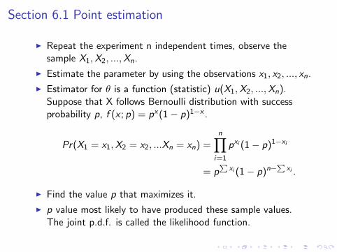
I Repeat the experiment n independent times, observe thesample X1,X2, ...,Xn.

I Estimate the parameter by using the observations x1, x2, ..., xn.

I Estimator for θ is a function (statistic) u(X1,X2, ...,Xn).Suppose that X follows Bernoulli distribution with successprobability p, f (x ; p) = px(1− p)1−x .

Pr(X1 = x1,X2 = x2, ...Xn = xn) =n∏

i=1

pxi (1− p)1−xi

= p∑

xi (1− p)n−∑

xi .

I Find the value p that maximizes it.

I p value most likely to have produced these sample values.The joint p.d.f. is called the likelihood function.


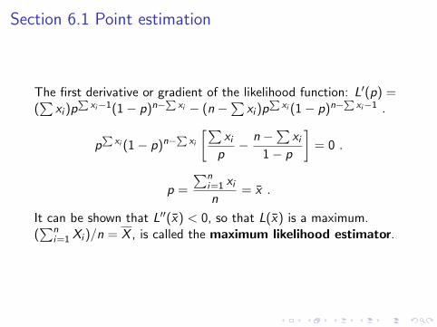
The first derivative or gradient of the likelihood function: L′(p) =(∑

xi )p∑

xi−1(1− p)n−∑

xi − (n −∑

xi )p∑

xi (1− p)n−∑

xi−1 .

p∑

xi (1− p)n−∑

xi

[∑xi

p− n −

∑xi

1− p

]= 0 .

p =

∑ni=1 xin

= x .

It can be shown that L′′(x) < 0, so that L(x) is a maximum.(∑n

i=1 Xi )/n = X , is called the maximum likelihood estimator.


When finding a maximum likelihood estimator, it is often easier tofind the value of the parameter that maximizes the naturallogarithm of the likelihood function rather than the value of theparameter that maximizes the likelihood function itself.

ln L(p) =

(n∑

i=1

xi

)ln p +

(n −

n∑i=1

xi

)ln(1− p) .

d [ln L(p)]

dp=

(n∑

i=1

xi

)(1

p

)+

(n −

n∑i=1

xi

)(−1

1− p

)= 0 ,


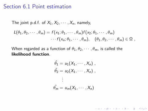
The joint p.d.f. of X1,X2, · · · ,Xn, namely,

L(θ1, θ2, · · · , θm) = f (x1; θ1, · · · , θm)f (x2; θ1, · · · , θm)

· · · f (xn; θ1, · · · , θm), (θ1, θ2, · · · , θm) ∈ Ω ,

When regarded as a function of θ1, θ2, · · · , θm, is called thelikelihood function.

θ1 = u1(X1, · · · ,Xn) ,

θ2 = u2(X1, · · · ,Xn) ,

...

θm = um(X1, · · · ,Xn)

Section 6.1 Point estimationExample 6.1-1

Let X1,X2, · · · ,Xn be a random sample from the exponentialdistribution with p.d.f.

f (x ; θ) =1

θe−x/θ, 0 < x <∞, θ ∈ Ω = θ : 0 < θ <∞ .

The likelihood function is given by

L(θ) = L(θ; x1, x2, · · · , xn)

=

(1

θe−x1/θ

)(1

θe−x2/θ

)· · ·(

1

θe−xn/θ

)=

1

θnexp

(−∑n

i=1 xiθ

), 0 < θ <∞ .

The natural logarithm of L(θ) is

ln L(θ) = −(n) ln(θ)− 1

θ

n∑i=1

xi , 0 < θ <∞ .


d [ln L(θ)]

dθ=−nθ

+

∑ni=1 xiθ2

= 0 .

The solution of this equation for θ is

θ =1

n

n∑i=1

xi = x .

Note that

d [ln L(θ)]

dθ=

1

θ

(−n +

nx

θ

) > 0, θ < x ,

= 0, θ = x ,

< 0, θ > x .

Hence, ln L(θ) does have a maximum at x , and it follows that themaximum likelihood estimator for θ is

θ = X =1

n

n∑i=1

Xi .

Section 6.1 Point estimationLet X1,X2, · · · ,Xn be a random sample from N(θ1, θ2), where

Ω = (θ1, θ2) : −∞ < θ1 <∞, 0 < θ2 <∞ .

That is, here we let θ1 = µ and θ2 = σ2. Then

L(θ1, θ2) =n∏

i=1

1√2πθ2

exp

[−(xi − θ1)2

2θ2

]or, equivalently,

L(θ1, θ2) =

(1√

2πθ2

)n

exp

[−∑n

i=1(xi − θ1)2

2θ2

], (θ1, θ2) ∈ Ω .

The natural logarithm of the likelihood function is

ln L(θ1, θ2) = −n

2ln(2πθ2)−

n∑i=1

(xi − θ1)2

2θ2.


The partial derivatives with respect to θ1 and θ2 are

∂(ln L)

∂θ1=

1

θ2

n∑i=1

(xi − θ1)

and∂(ln L)

∂θ2=−n2θ2

+1

2θ22

n∑i=1

(xi − θ1)2 .

The equation ∂(ln L)/∂θ1 = 0 has the solution θ1 = x . Setting∂(ln L)/∂θ2 = 0 and replacing θ1 by x yields

θ2 =1

n

n∑i=1

(xi − x)2 .


By considering the usual condition on the second partialderivatives, we see that these solutions do provide a maximum.Thus, the maximum likelihood estimators of µ = θ1 and σ2 = θ2

are

θ1 = X and θ2 =1

n

n∑i=1

(Xi − X )2 = V .

It is interesting to note that in our first illustration, where p = X ,and in Example 6.1-1, where θ = X , the expected value of theestimator is equal to the corresponding parameter. Thisobservation leads to the following definition.


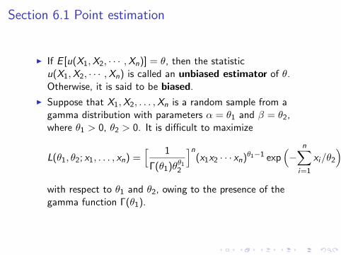
I If E [u(X1,X2, · · · ,Xn)] = θ, then the statisticu(X1,X2, · · · ,Xn) is called an unbiased estimator of θ.Otherwise, it is said to be biased.

I Suppose that X1,X2, . . . ,Xn is a random sample from agamma distribution with parameters α = θ1 and β = θ2,where θ1 > 0, θ2 > 0. It is difficult to maximize

L(θ1, θ2; x1, . . . , xn) =[ 1

Γ(θ1)θθ12

]n(x1x2 · · · xn)θ1−1 exp

(−

n∑i=1

xi/θ2

)with respect to θ1 and θ2, owing to the presence of thegamma function Γ(θ1).


I (Moment method) Equating the sample moment(s) to thetheoretical moment(s).

I For gamma distribution:

θ1θ2 = X , θ1θ22 = V ,

θ1 =X

2

Vand θ2 =

V

X.

θ1 and θ2, are respective estimators of θ1 and θ2 found by themethod of moments.

I The sum Mk =∑n

i=1 Xki /n is the kth moment of the sample,

k = 1, 2, 3, . . .. The method of moments can be described asfollows: Equate E (X k) to Mk .

Section 6.1 Point estimationExample 6.1-6

Let the distribution of X be N(µ, σ2). Then

E (X ) = µ and E (X 2) = σ2 + µ2 .

For a random sample of size n, the first two moments are given by

m1 =1

n

n∑i=1

xi and m2 =1

n

n∑i=1

x2i .

We set m1 = E (X ) and m2 = E (X 2) and solve for µ and σ2. Thatis,

1

n

n∑i=1

xi = µ and1

n

n∑i=1

x2i = σ2 + µ2 .

The first equation yields x as the estimate of µ.


Replacing µ2 with x2 in the second equation and solving for σ2, weobtain

1

n

n∑i=1

x2i − x2 =

n∑i=1

(xi − x)2

n= v

as the solution of σ2. Thus, the method-of-moments estimators forµ and σ2 are µ = X and σ2 = V , which are the same as themaximum likelihood estimators. Of course, µ = X is unbiased

whereas σ2 = V is biased.

Section 6.2 Confidence intervals for means

I A random sample X1,X2, . . . ,Xn from a normal distributionN(µ, σ2), and σ2 is known;

I X is N(µ, σ2/n)

P(− zα/2 ≤

X − µσ/√n≤ zα/2

)= 1− α .

−zα/2 ≤X − µσ/√n≤ zα/2 ,

X + zα/2

( σ√n

)≥ µ ≥ X − zα/2

( α√n

).


I

P[X − zα/2

( σ√n

)≤ µ ≤ X + zα/2

( σ√n

)]= 1− α .

I The probability that the random interval[X − zα/2

( σ√n

), X + zα/2

( σ√n

)]includes the unknown mean µ is 1− α. A 100(1− α)%confidence interval for the unknown mean µ. A shorterconfidence interval indicates that we have more credence in xas an estimate of µ.


If we cannot assume that the distribution from which the samplearose is normal. By the central limit theorem, provided that n islarge enough, the ratio (X − µ)/(σ/

√n) has the approximate

normal distribution N(0, 1) when the underlying distribution is notnormal.

P(− zα/2 ≤

X − µσ/√n≤ zα/2

)≈ 1− α .

and [x − zα/2

( σ√n

), x + zα/2

( σ√n

)]is an approximate 100(1− α)% confidence interval for µ. Whenthe underlying distribution is unimodal (has only one mode) andcontinuous, the approximation is usually quite good even for smalln, such as n = 5. In almost all cases, an n of at least 30 is usuallyadequate.


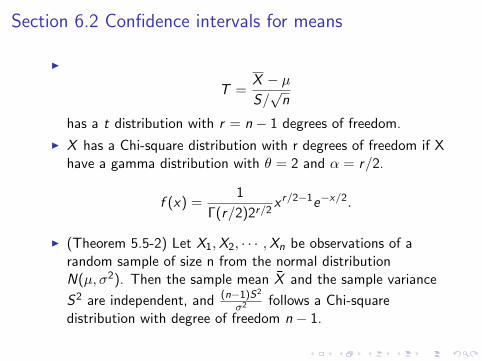
I

T =X − µS/√n

has a t distribution with r = n − 1 degrees of freedom.

I X has a Chi-square distribution with r degrees of freedom if Xhave a gamma distribution with θ = 2 and α = r/2.

f (x) =1

Γ(r/2)2r/2x r/2−1e−x/2.

I (Theorem 5.5-2) Let X1,X2, · · · ,Xn be observations of arandom sample of size n from the normal distributionN(µ, σ2). Then the sample mean X and the sample variance

S2 are independent, and (n−1)S2

σ2 follows a Chi-squaredistribution with degree of freedom n − 1.


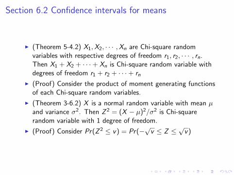
I (Theorem 5-4.2) X1,X2, · · · ,Xn are Chi-square randomvariables with respective degrees of freedom r1, r2, · · · , rn.Then X1 + X2 + · · ·+ Xn is Chi-square random variable withdegrees of freedom r1 + r2 + · · ·+ rn

I (Proof) Consider the product of moment generating functionsof each Chi-square random variables.

I (Theorem 3-6.2) X is a normal random variable with mean µand variance σ2. Then Z 2 = (X − µ)2/σ2 is Chi-squarerandom variable with 1 degree of freedom.

I (Proof) Consider Pr(Z 2 ≤ v) = Pr(−√v ≤ Z ≤

√v)


I (Theorem 5-5.3) Let

T =Z√U/r

where Z is the standard normal random variable with meanzero and variance 1, U is another independent randomvariable following a Chi-square distribution with degree offreedom r. Then T has a t-distribution with p.d.f

f (t) =Γ((r + 1)/2)√πrΓ(r/2)

1

(1 + t2/r)(r+1)/2

I (Proof) ConsiderF (t) = Pr(Z/

√U/r ≤ t) = Pr(Z ≤

√U/r t)


Select tα/2(n − 1) so that P[T ≥ tα/2(n − 1)] = α/2.

1− α = P[− tα/2(n − 1) ≤ X − µ

S/√n≤ tα/2(n − 1)

]= P

[X − tα/2(n − 1)

( S√n

)≤ µ ≤ X + tα/2(n − 1)

( S√n

)].

[x − tα/2(n − 1)

( s√n

), x + tα/2(n − 1)

( s√n

)]is a 100(1− α)% confidence interval for µ.


I Not able to assume that the underlying distribution is normal,approximate confidence intervals for µ can still be constructedwith the formula

T =X − µS/√n,

which now only has an approximate t distribution, it workswell if the underlying distribution is symmetric, unimodal, andof the continuous type.

I Assume the variance is known. Once X is observed to beequal to x , it follows that [x − zα(σ/

√n),∞) is a

100(1− α)% one-sided confidence interval for µ.

Section 6.3 Confidence intervals for the difference of 2means

I Two independent sample X1,X2, · · · ,Xn and Y1,Y2, · · · ,Ym

with respective distributions N(µX , σ2X ), N(µY , σ

2Y ).

I Both variance are assumed to be known.

I Distribution of the difference W = X − Y isN(µX − µY , σ2

X/n + σ2Y /m)

I [x − y − zα/2σW , x − y + zα/2σW ] serves as a 100(1− α)%confidence interval for the difference of 2 means.

I If the sample sizes are large, while both variance are unknown,we can replace the population variance with the sample

variances, and x − y ± zα/2

√s2x /n + s2

y /m serves as an

approximate 100(1− α)% confidence interval for thedifference of 2 means.


I Small sample (< 30) yet with a common variance

I Z = X−Y−(µx−µY )√σ2/n+σ2/m

is N(0, 1)

I U =(n−1)S2

Xσ2 +

(m−1)S2Y

σ2 is χ2(n + m − 2).

I T = Z√U/(n+m−2)

has a t-distribution with n + m − 2 degrees

of freedom

I Set t0 = tα/2(n + m − 2) and SP =

√(n−1)S2

X +(m−1)S2Y

n+m−2

I x − y ± t0sP√

1/n + 1/m is a 100(1− α)% confidenceinterval for the difference of 2 means.

I Notice that when both n and m are large, T ≈ X−Y−(µx−µY )√S2X /m+S2

Y /n,

i.e. each variance is divided by a wrong sample size.


I Small sample with different variances

I

1

r=

c2

n − 1+

(1− c)2

m − 1I

c =s2x /n

s2x /n + s2

y /m

I x − y ± tα/2(r)√

s2x /n + s2

y /m is a 100(1− α)% confidence

interval for the difference of 2 means.


I X and Y are dependent, e.g. weight before and afterparticipating in a diet-and-exercise program.

I Let (X1,Y1), (X2,Y2), · · · , (Xn,Yn) be n pairs of dependentmeasurements.

I Di ≡ Xi − Yi form a random sample from N(µD , σ2D).

I Use T = D−µDSD/√n

as test statistics.

Section 6.4 Confidence intervals for variances

I The distribution of (n − 1)S2/σ2 is χ2(n − 1)

I

P

(a ≤ (n − 1)S2

σ2≤ b

)= 1− α .

I Selecting a and b so that a = χ21−α/2(n − 1) and

b = χ2α/2(n − 1)

I

1− α = P

(a

(n − 1)S2≤ 1

σ2≤ b

(n − 1)S2

)= P

((n − 1)S2

b≤ σ2 ≤ (n − 1)S2

a

).

I a 100(1− α)% confidence interval for σ, the standarddeviation, is given by[√

(n − 1)s2

b,

√(n − 1)s2

a

]=

[√n − 1

bs,

√n − 1

as

].


I (Example 5-2.4) F = U/r1

V /r2where U and V are independent

chi-square random variables with respective degrees offreedom r1 and r2. Then we said F has an F-distribution withthe same degrees of freedom and its p.d.f. is

f (w) =(r1/r2)r1/2Γ[(r1 + r2)/2]w r1/2−1

Γ(r1/2)Γ(r2/2)[1 + (r1w/r2)](r1+r2)/2

I (Proof) First write down the joint density, and then use thedefinition

F (w) = Pr(U/r1V /r2

≤ w) = Pr(U ≤ r1r2Vw)


I Two independent sample X1,X2, · · · ,Xn and Y1,Y2, · · · ,Ym

with respective distributions N(µX , σ2X ), N(µY , σ

2Y ).

I (n − 1)S2X/σ

2X and (m − 1)S2

Y /σ2Y are independent chi-square

variables with (n − 1) and (m − 1) degrees of freedom

I

F =

(m − 1)S2Y

σ2Y (m − 1)

(n − 1)S2X

σ2X (n − 1)

=

S2Y

σ2Y

S2X

σ2X

I F has an F distribution with r1 = m − 1 and r2 = n − 1degrees of freedom

1− α = P

(c ≤

S2Y /σ

2Y

S2x /σ

2x

≤ d

)= P

(cS2X

S2Y

≤σ2X

σ2Y

≤ dS2X

S2Y

).


I

1− α = P

(c ≤

S2Y /σ

2Y

S2x /σ

2x

≤ d

)= P

(cS2X

S2Y

≤σ2X

σ2Y

≤ dS2X

S2Y

).

I If s2x and s2

y are the observed values of S2X and S2

Y ,respectively, then[

1

Fα/2(n − 1,m − 1)

s2x

s2y

,Fα/2(m − 1, n − 1)s2x

s2y

]is a 100(1− α) % confidence interval for σ2

X/σ2Y .

I These intervals are generally not too useful because they areoften very wide. The confidence coefficients are not veryaccurate if we deviate much from underlying normaldistributions.

Section 6.5 Confidence intervals for proportions

I Let Y equal the frequency of measurements in the intervalout of the n observations

I Y has the binomial distribution b(n, p)

I To determine the accuracy of the relative frequency Y /n asan estimator of p

IY − np√np(1− p)

=(Y /n)− p√p(1− p)/n

has an approximate normal distribution N(0, 1).

I

P

[−zα/2 ≤

(Y /n)− p√p(1− p)/n

≤ zα/2

]≈ 1− α


I (Method I) Replacing p with Y /n in p(1− p)/n in theendpoints[

y

n− zα/2

√(y/n)(1− y/n)

n,y

n+ zα/2

√(y/n)(1− y/n)

n

]

serves as an approximate 100(1− α)% confidence interval forp


I (Method II)|Y /n − p|√p(1− p)/n

≤ zα/2

is equivalent to

H(p) =

(Y

n− p

)2

−z2α/2p(1− p)

n≤ 0

Letting p = Y /n and z0 = zα/2

H(p) =

(1 +

z20

n

)p2 −

(2p +

z20

n

)p + p2 .

p + z20/(2n)± z0

√p(1− p)/n + z2

0/(4n2)

1 + z20/n


I Statistical inference about the difference p1 − p2

I Y1/n1 − Y2/n2 must have mean p1 − p2 and variance

p1(1− p1)

n1+

p2(1− p2)

n2.

I(Y1/n1)− (Y2/n2)− (p1 − p2)√p1(1− p1)/n1 + p2(1− p2)/n2

has an approximate normal distribution N(0, 1).

I For large n1 and n2, replace p1 and p2 in the denominator ofthis ratio by Y1/n1 and Y2/n2, respectively

I An approximate 100(1− α)% confidence interval

y1

n1− y2

n2± zα/2

√(y1/n1)(1− y1/n1)

n1+

(y2/n2)(1− y2/n2)

n2

for the unknown difference p1 − p2

Section 6.6 Sample sizeI How large should the sample size be to estimate a mean? In

general, the smaller the variance, the smaller is the samplesize needed to achieve to given degree of accuracy

I (Example 6-6.1) A mathematics department wishes toevaluate a new method of teaching calculus with a computer.

I Aim to find the sample size n such that we are fairly confidentthat x ± 1 contains the unknown test mean µ. From pastexperience, it is believed that the standard deviationassociated with this type of test is about 15

I X is approximately N(µ, σ2/n)I x ± 1.96(15/

√n) will serve as an approximate 95% confidence

interval for µI

1.96

(15√n

)= 1

√n = 29.4 and thus n ≈ 864.36 ,

or n = 865 because n must be an integer

Section 6.6 Sample sizeI Less ambitious plan: x ± 2 would be a satisfactory 80% one

1.282

(15√n

)= 2

or, equivalently,√n = 9.615 so that n ≈ 92.4 .

n must be an integer, we prefer to use 93 instead.I In general, to find the 100(1− α)% confidence interval forµ, x ± zα/2(σ/

√n), to be no longer than that given by x ± ε,

set up equation:

ε =zα/2σ√

n, where Φ(zα/2) = 1− α

2.

That is,

n =z2ασ

2

ε2

where it is assumed that σ2 is known.

Section 6.6 Sample size

I To find the required sample size to estimate the proportion p.

I The point estimate of p is p = y/n

I an approximate 1− α confidence interval for p is

p ± zα/2

√p(1− p)

n.

I p is unknown before the experiment is run, we cannot use thevalue of p in our determination of n.

I No matter what value p takes between 0 and 1, it is alwaystrue that p∗(1− p∗) ≤ 1/4

n =z2α/2p

∗(1− p∗)

ε2≤

z2α/2

4ε2.

And now pick n =z2α/2

4ε2

Section 6.6 Sample size

I Finite population size

I Let N1 individuals in a population of size N havecharacteristic C. Let p = N1/N.

I Take a sample of size n without replacement, the number ofobservations X with the characteristic C, has ahypergeometric distribution. Recall (see Examples 2-2.5 and2-3.5 for details) the mean and the variance of X are:

µ = n(N1

N) = np

σ2 = nN1

N(1− N1

N)(N − n

N − 1) = np(1− p)(

N − n

N − 1)

Section 6.6 Sample sizeI

E (X

n) =

µ

n= p

Var(X

n) =

σ2

n2=

p(1− p)

n(N − n

N − 1)

I An approximate 1− α confidence interval for p is

p ± zα/2

√p(1− p)

n(N − n

N − 1)

where p = x/nI Let ε be the maximum error of the estimate of p

ε = zα/2

√p(1− p)

n(N − n

N − 1)

n =m

1 + m−1N

which is an increasing function of m, and we substitute

m =z2α/2

p∗(1−p∗)

ε2 and we pick p∗ = 1/2.

Section 6.7 Simple regression

I For any random variable Y , even though we cannot predict itsfuture observed value Y = y with certainty, we can stillestimate its mean.

I Suppose that E (Y ) is a function of another observed variablex . E (Y ) = µ(x) is assumed to be of a given form, such aslinear, quadratic, or exponential: µ(x) could be assumed to beequal to α + βx , α + βx + γx2, or αeβx

I Firstly, consider the case that E (Y ) = µ(x) is a linear function

I Given (x1, y1), (x2, y2), · · · , (xn, yn), we like to fit a straightline to the set of data

Yi = α1 + βxi + εi ,

where εi , for i = 1, 2, · · · , n, are independent and N(0, σ2)


I Y1,Y2, · · · ,Yn are mutually independent normal variableswith respective means α + β(xi − x), i = 1, 2, · · · , n, andunknown variance σ2, where α = α1 + βx


I The likelihood function

L(α, β, σ2) =n∏

i=1

1√2πσ2

exp

− [yi − α− β(xi − x)]2

2σ2

=

(1

2πσ2

)n/2

exp

−∑n

i=1[yi − α− β(xi − x)]2

2σ2

.

I To maximize L(α, β, σ2) or, equivalently, to minimize

− ln L(α, β, σ2) =n

2ln(2πσ2) +

n∑i=1

[yi − α− β(xi − x)]2

2σ2,

we must select α and β to minimize

H(α, β) =n∑

i=1

[yi − α− β(xi − x)]2 .


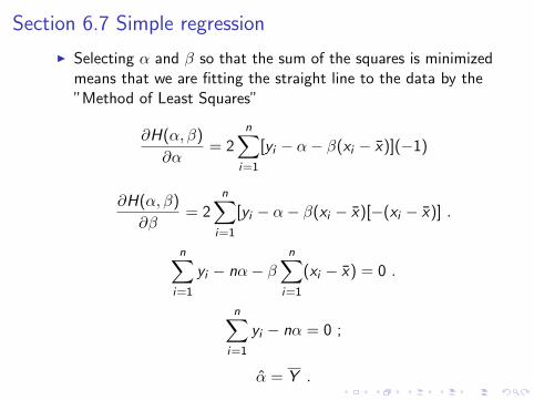
I Selecting α and β so that the sum of the squares is minimizedmeans that we are fitting the straight line to the data by the”Method of Least Squares”

∂H(α, β)

∂α= 2

n∑i=1

[yi − α− β(xi − x)](−1)

∂H(α, β)

∂β= 2

n∑i=1

[yi − α− β(xi − x)[−(xi − x)] .

n∑i=1

yi − nα− βn∑

i=1

(xi − x) = 0 .

n∑i=1

yi − nα = 0 ;

α = Y .


I The equation ∂H(α, β)/∂β = 0 yields

n∑i=1

(yi − Y )(xi − x)− βn∑

i=1

(xi − x)2 = 0

β =

n∑i=1

(Yi − Y )(xi − x)

n∑i=1

(xi − x)2

=

n∑i=1

Yi (xi − x)

n∑i=1

(xi − x)2

.

∂[− ln L(α, β, σ2)]

∂(σ2)=

n

2σ2−

n∑i=1

[yi − α− β(xi − x)]2

2(σ2)2.

σ2 =1

n

n∑i=1

[Yi − α− β(xi − x)]2

I The maximum likelihood estimate of σ2 is then the sum ofthe squares of the residuals divided by n.

Section 6.7 Simple regressionI Both α and β are linear functions of Y1,Y2, · · · ,Yn, and

hence have normal distributions with respective means andvariances:

E (α) = E

(1

n

n∑i=1

Yi

)=

1

n

n∑i=1

E (Yi ) = α

Var(α) =n∑

i=1

(1

n

)2

Var(Yi ) =σ2

n.

E (β) =

n∑i=1

(xi − x)E (Yi )∑ni=1(xi − x)2

=

n∑i=1

(xi − x)[α + β(xi − x)]

n∑i=1

(xi − x)2

=

αn∑

i=1(xi − x) + β

n∑i=1

(xi − x)2

n∑i=1

(xi − x)2

= β


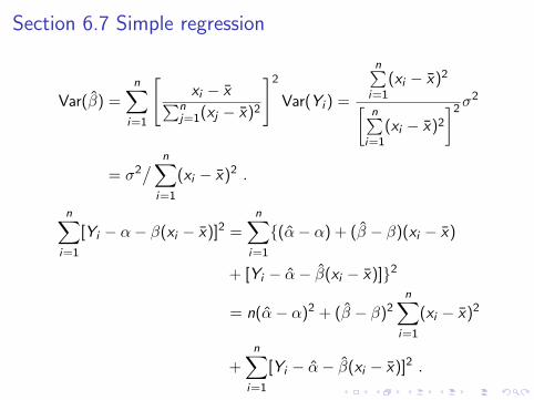
Var(β) =n∑

i=1

[xi − x∑n

j=1(xj − x)2

]2

Var(Yi ) =

n∑i=1

(xi − x)2

[n∑

i=1(xi − x)2

]2σ2

= σ2/ n∑

i=1

(xi − x)2 .

n∑i=1

[Yi − α− β(xi − x)]2 =n∑

i=1

(α− α) + (β − β)(xi − x)

+ [Yi − α− β(xi − x)]2

= n(α− α)2 + (β − β)2n∑

i=1

(xi − x)2

+n∑

i=1

[Yi − α− β(xi − x)]2 .

Section 6.7 Simple regressionI Yi , α, and β have normal distributions, and hence each of

[Yi − α− β(xi − x)]2

σ2,

(α− α)2[σ2

n

] , and(β − β)2

σ2∑ni=1(xi − x)2

has a chi-square distribution with one degree of freedom.I Therefore,

n∑i=1

[Yi − α− β(xi − x)]2

σ2

is χ2(n).

I It can be shown that α, β, and σ2 are mutually independent(see Hogg, McKean and Craig [2005]). Therefore,

n∑i=1

[Yi − α− β(xi − x)]2

σ2=

nσ2

σ2≥ 0 .

is χ2(n − 2).


I Therefore, we deduce that

T1 =

√n∑

i=1(xi − x)2

(β − βσ

)√

nσ2

σ2(n − 2)

=β − β√nσ2

(n − 2)∑n

i=1(xi − x)2

has a t distribution with n − 2 degrees of freedom.

I Let

η =

√nσ2

(n − 2)∑n

i=1(xi − x)2[β − tγ/2(n − 2)η, β + tγ/2(n − 2)η

]is a 100(1− γ)% confidence interval for β, where


I Similarly,

T2 =

√n(α− α)

σ√nσ2

σ2(n − 2)

=α− α√σ2

n − 2

has a t distribution with n − 2 degrees of freedom.

I The fact that nσ2/σ2 has a chi-square distribution with n − 2degrees of freedom can be used to make inferences about thevariances σ2

Section 6.8 More regression

I For a given x , Y = α + β(x − x) is a point estimate for themean of Y . Since α and β are normally and independentlydistributed, Y has a normal distribution.

E (Y ) = E [α + β(x − x)]

= α + β(x − x)

Var(Y ) = Var[α + β(x − x)]

=σ2

n+

σ2∑ni=1(xi − x)2

(x − x)2

= σ2

[1

n+

(x − x)2∑ni=1(xi − x)2

].


I Since α and β are independent of σ2,

T =

α + β(x − x)− [α + β(x − x)]

σ

√1

n+

(x − x)2∑ni=1(xi − x)2√nσ2

(n − 2)σ2

,


I Let

c =

√nσ2

n − 2

√1

n+

(x − x)2∑ni=1(xi − x)2

.

The endpoints for a 100(1− γ)% confidence interval forµ(x) = α + β(x − x) are

α + β(x − x)± ctγ/2(n − 2) .

Section 6.8 More regressionI A prediction interval for Yn+1 when x = xn+1:

W = Yn+1 − α− β(xn+1 − x)

is a linear combination of normally and independentlydistributed random variables, so W has a normal distribution.

E (W ) = E [Yn+1 − α− β(xn+1 − x)]

= α + β(xn+1 − x)− α− β(xn+1 − x) = 0 .

I Since Yn+1, α and β are independent, the variance of W is

Var(W ) = σ2 +σ2

n+

σ2

n∑i=1

(xi − x)2

(xn+1 − x)2

= σ2

1 +1

n+

(xn+1 − x)2

n∑i=1

(xi − x)2

.


I Yn+1, α, and β are independent of σ2,

T =

Yn+1 − α− β(xn+1 − x)

σ

√1 +

1

n+

(xn+1 − x)2∑ni=1(xi − x)2√

nσ2

(n − 2)σ2


I Let

d =

√nσ2

n − 2

√1 +

1

n+

(xn+1 − x)2∑ni=1(xi − x)2

.

The endpoints for a 100(1− γ)% prediction interval for Yn+1

areα + β(xn+1 − x)± dtγ/2(n − 2) .

The end of Chapter 6

Documents

Theory of Point Estimation - Statistics notes of STA 2006/Chapter6.pdf · Theory of Point Estimation Dr. Phillip YAM 2012/2013 Spring Semester Reference: Chapter 6 of \Probability