Embed Size (px)
Citation preview

Estimation Of
Point,
Interval and
Sample Size.
THEORY OF
ESTIMATION
9/3/20121

INTRODUCTION: Estimation Theory is a procedure of “guessing”
properties of the population from which data are
collected.
i.e, The objective of estimation is to determine the
approximate value of a population parameter on the
basis of a sample statistic.
An estimator is a rule, usually a formula, that tells
you how to calculate the estimate based on the
sample.
9/3/20122
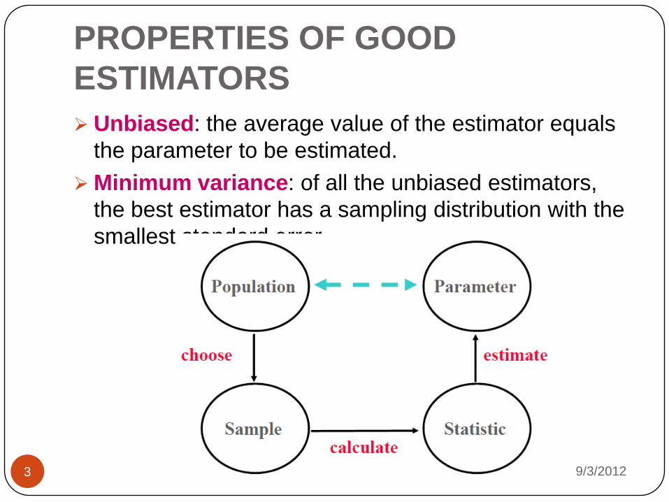
PROPERTIES OF GOOD
ESTIMATORS
Unbiased: the average value of the estimator equals
the parameter to be estimated.
Minimum variance: of all the unbiased estimators,
the best estimator has a sampling distribution with the
smallest standard error.
9/3/20123
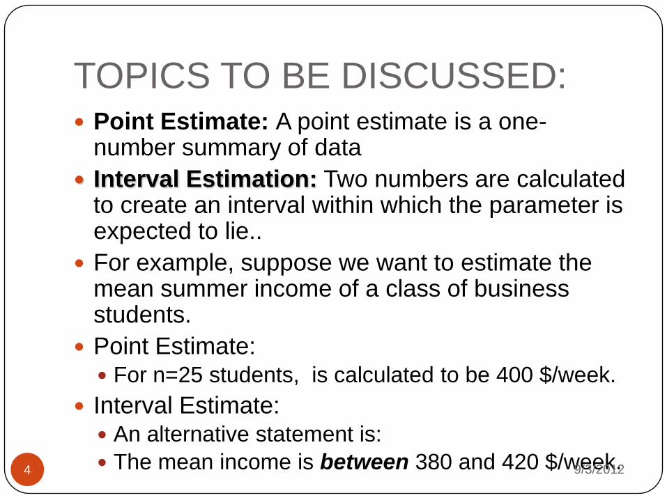
TOPICS TO BE DISCUSSED: Point Estimate: A point estimate is a one-
number summary of data
Interval Estimation: Two numbers are calculated to create an interval within which the parameter is expected to lie..
For example, suppose we want to estimate the mean summer income of a class of business students.
Point Estimate: For n=25 students, is calculated to be 400 $/week.
Interval Estimate: An alternative statement is:
The mean income is between 380 and 420 $/week.9/3/20124

Sample Size
"Sample Size" - is the number of a population
that will be evaluated as representing the
entire population, and from which statistics will
be derived.
The sample size is an important feature of
any empirical study in which the goal is to
make inferences about a population from a
sample.
In practice, the sample size used in a study is
determined based on the expense of data
collection, and the need to have sufficient
statistical power .9/3/20125
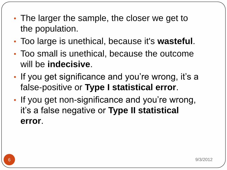
• The larger the sample, the closer we get to
the population.
• Too large is unethical, because it's wasteful.
• Too small is unethical, because the outcome
will be indecisive.
• If you get significance and you’re wrong, it’s a
false-positive or Type I statistical error.
• If you get non-significance and you’re wrong,
it’s a false negative or Type II statistical
error.
9/3/20126

Factors That Influence Sample Size
• The "right" sample size for a particular application depends on many factors, including the following:
• Cost considerations (e.g., maximum budget, desire to minimize cost).
• Administrative concerns (e.g., complexity of the design, research deadlines).
• Minimum acceptable level of precision.
• Confidence level.
• Variability within the population or subpopulation (e.g., stratum, cluster) of interest.
• Sampling method. 9/3/20127
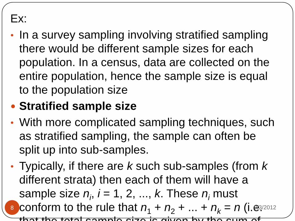
Ex:
• In a survey sampling involving stratified sampling
there would be different sample sizes for each
population. In a census, data are collected on the
entire population, hence the sample size is equal
to the population size
Stratified sample size
• With more complicated sampling techniques, such
as stratified sampling, the sample can often be
split up into sub-samples.
• Typically, if there are k such sub-samples (from k
different strata) then each of them will have a
sample size ni, i = 1, 2, ..., k. These ni must
conform to the rule that n1 + n2 + ... + nk = n (i.e.
that the total sample size is given by the sum of
9/3/20128

ESTIMAION OF SAMPLE
POINT: A single number is calculated to estimate the
parameter.
A point estimate is obtained by selecting a suitable
statistic and computing its value from the given
sample data. The selected statistic is called the point
estimator of θ.
A point estimate of an unknown parameter is a statistic
that represents a “guess” at the value of .
Parameters
In statistical inference, the term parameter is used
to denote a quantity , say, that is a property of an
unknown probability distribution.
Parameters are unknown, and one of the goals of
statistical inference is to estimate them.
9/3/20129

Example (Machine breakdowns)
Estimating
P(machine breakdown due to operator misuse).
Some general Concepts of Point Estimation:
Unbiasedness.
Principle of Minimum Variance.
Methods of Point Estimation:
Maximum Likelihood Estimation.
The Method of Moments.
9/3/201210

Point Estimator Of Population
Mean
A sample of weights of 34 male freshman students was obtained.
185 161 174 175 202 178 202 139 177
170 151 176 197 214 283 184 189 168
188 170 207 180 167 177 166 231 176
184 179 155 148 180 194 176If one wanted to estimate the true mean of all male freshman students,
you might use the sample mean as a point estimate for the true mean.
sample mean x 182.44
n
xx i
A point estimate of population mean is the
sample mean
9/3/201211

BIASED & UNBIASED
A point estimate for a parameter is said to
be
unbiased if
If this equality does not hold, is said to be a
biased estimator of θ, with
ˆ( )E
ˆ ( )bias E
9/3/201212

Variance of a Point Estimator
The sampling distributions oftwo unbiased estimators.
Of all the unbiasedestimators, we prefer theestimator whose samplingdistribution has the smallestspread or variability.
9/3/201213
INTERVAL ESTIMATES An Estimation of a population parameter given
by two numbers between which the parameter may
be called as an internal estimation of the
parameter.
Eg : If we say that a distance is 5.28 feet, we are
giving a point estimate. If, on the other hand, we
say that the distance is 5.28 ± 0.03 feet, i.e., the
distance lies between 5.25 and 5.31 feet, we are
giving an interval estimate.
A statement of the error or precision of an
estimate is often called its reliability.
9/3/201214

CONFIDENCE INTERVAL ESTIMATES
OF POPULATION PARAMETERS
Let μS and σS be the mean and standard
deviation of the sampling distribution of a
statistic S.
Then, if the sampling distribution of S is
approximately normal we can expect to find S
lying in the interval μS . σS to μS + σS, μS . 2σS
to μS + 2σS or μS . 3σS to μS + 3σS about
68.27%, 95.45%, and 99.73% of the time,
respectively.
We can be con.dent of .nding μS in the intervals
S. σS to S + σS, S . 2σS to S + 2σS, or S . 3σS
to S + 3σS about 68.27%, 95.45%, and 99.73%
of the time, respectively. Because of this, we call
9/3/201215
CONFIDENCE LIMITS: The end numbers of these intervals (S ± σS, S ± 2 σS, S ±
3 σS) are then called the 68.37%, 95.45%, and 99.73%
Confidence Limits.
CONFIDENCE LEVEL : S ± 1.96 σS and S ± 2.58 σS are 95% and 99% (or 0.95
and0.99) confidence limits for μS. The percentage
confidence is often called Confidence Level.
CRITICAL VALUE :
The numbers 1.96, 2.58, etc., in the confidence
limits are called Critical Values, and are denoted
by zC. From confidence levels we can find critical
values.9/3/201216

Eg:
we give values of zC corresponding to various
confidence levels used in practice. For confidence
levels not presented in the table, the values of zC can
be found from the normal curve areas under the
Standard Normal Curve from 0 to z.
C L 99.7% 99% 98
%
96% 95.45
%
95% 90% 80% 68.27
%
3.00 2.58 2.3
3
2.05 2.00 1.96 1.645 1.28 1.00
9/3/201217
In cases where a statistic has a sampling distribution
that is different from the normal distribution,
appropriate modifications to obtain confidence intervals
have to be made.
CONFIDENCE INTERVALS:
Confidence Intervals for Means
Confidence Intervals for Proposition
Confidence Intervals for Differences and Sums.
9/3/201218
Confidence Intervals for
Means :
We shall see how to create confidence intervals
for the mean of a population using two different
cases.
The first case shall be when we have a Large
Sample Size (N ≥ 30).
The second case shall be when we have a
Smaller Sample (N < 30).
Then Underlying Population is normal.
9/3/201219

Large Samples (n ≥ 30) : If the statistic S is the sample mean X, then the
95% and 99% confidence limits for estimation of
the population mean μ are given by X ±1.96 σX
and X ± 2.58 σX, respectively.
The confidence limits are given by X ± zc σX
where zc, which depends on the particular level
of confidence desired.
9/3/201220

In case sampling from an infinite
population or if sampling is done with
replacement from a finite population,
and by
•If sampling is done without replacement
from a population of finite size N.
•The population standard deviation σis
unknown, so that to obtain the above
confidence limits, we use the estimator
Sˆ or S.9/3/201221

Small Samples (n < 30) and
Population Normal :• We use the t distribution to obtain confidence
levels. For example, if –t0.975 and t0.975 are
the values of T for which 2.5% of the area lies
in each tail of the t distribution, then a 95%
confidence interval for T is given by
from which we can see that μ can be
estimated to lie in the interval with 95%
confidence.
9/3/201222
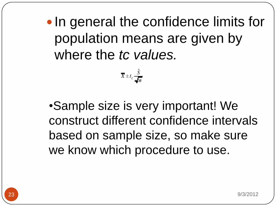
In general the confidence limits for
population means are given by
where the tc values.
•Sample size is very important! We
construct different confidence intervals
based on sample size, so make sure
we know which procedure to use.
9/3/201223
Confidence Intervals for
Proportions :
The statistic S is the proportion of “successes”
in a sample of size n ≥ 30 drawn from a
binomial population in which p is the proportion
of successes.
Then the confidence limits for p are given by P
± zc σP, where P denotes the proportion of
success in the sample of size n. Using the
values of σP obtained, we see that the
confidence limits for the population proportion
are given by 9/3/201224
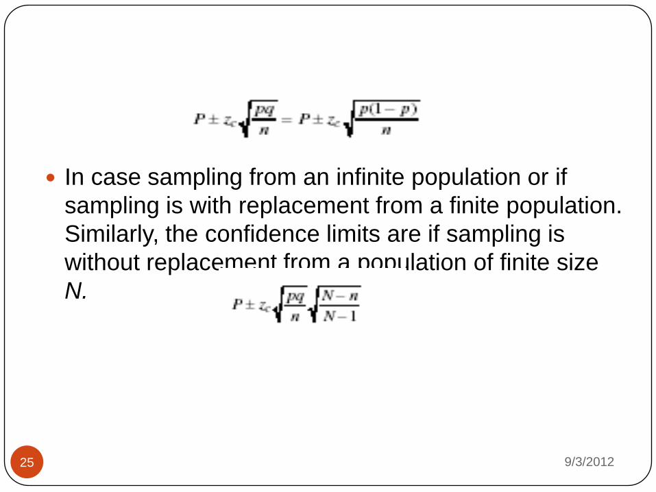
In case sampling from an infinite population or if
sampling is with replacement from a finite population.
Similarly, the confidence limits are if sampling is
without replacement from a population of finite size
N.
9/3/201225
Confidence Intervals for
Differences and Sums :
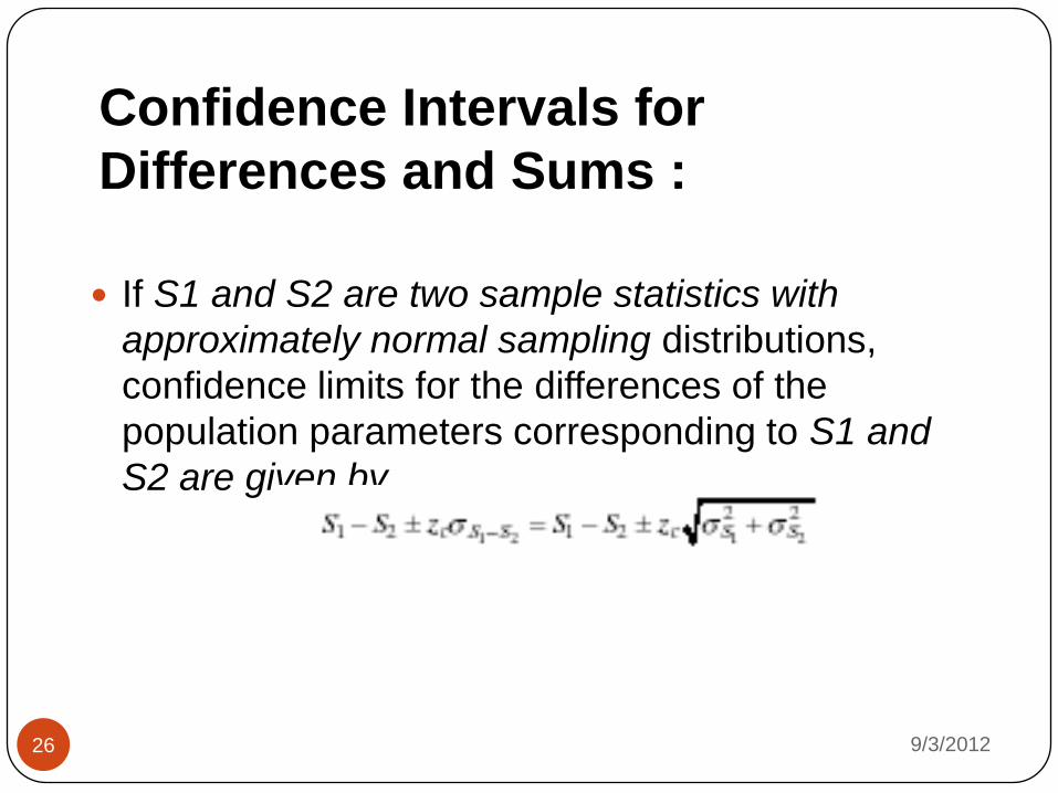
If S1 and S2 are two sample statistics with
approximately normal sampling distributions,
confidence limits for the differences of the
population parameters corresponding to S1 and
S2 are given by
9/3/201226
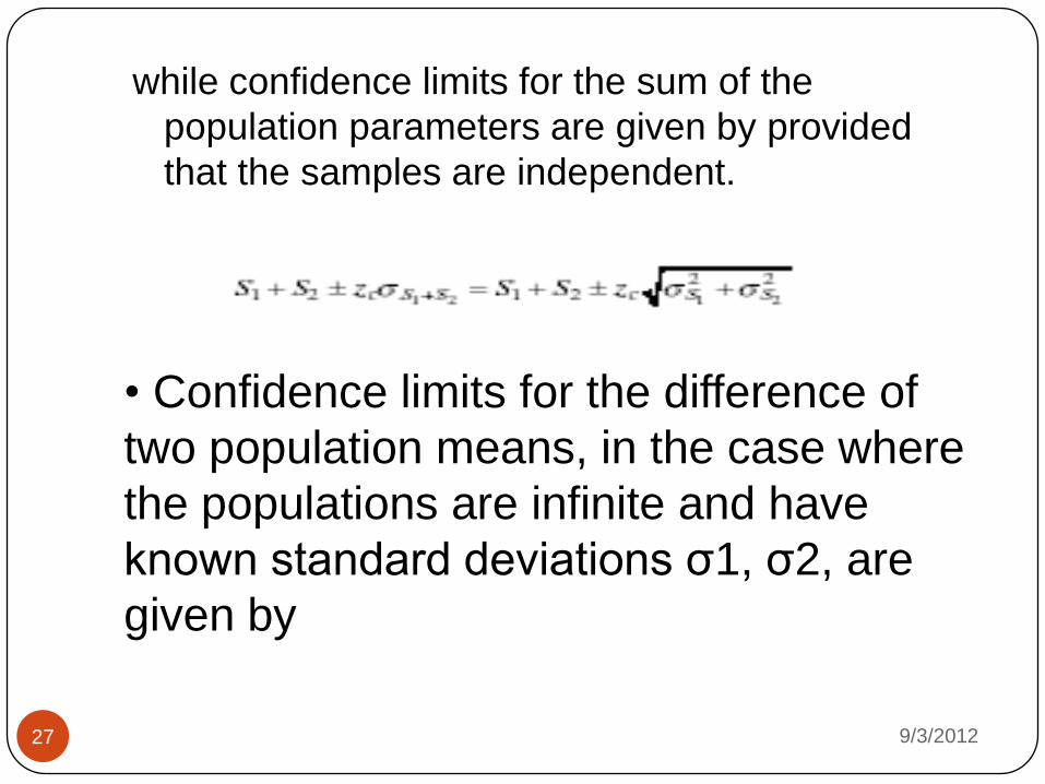
while confidence limits for the sum of the
population parameters are given by provided
that the samples are independent.
• Confidence limits for the difference of
two population means, in the case where
the populations are infinite and have
known standard deviations σ1, σ2, are
given by
9/3/201227

Where are the
respective means and sizes of the two
samples drawn from the populations.
Confidence limits for the difference of two
population proportions, where the
populations are infinite, are given by
9/3/201228
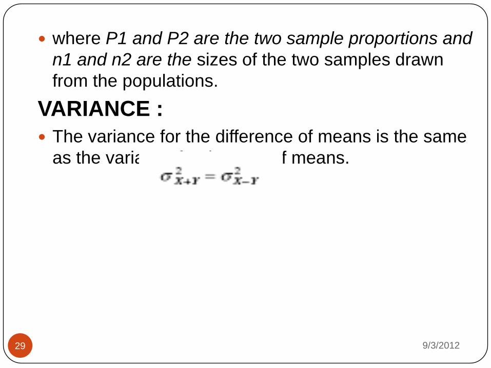
where P1 and P2 are the two sample proportions and
n1 and n2 are the sizes of the two samples drawn
from the populations.
VARIANCE :
The variance for the difference of means is the same
as the variance for the sum of means.
9/3/201229

9/3/201230

![ESTIMATION THEORY - The Open Academy · [Kay’93] S. M. Kay, Fundamentals of Statistical Signal Processing: Estimation Theory, ... we use one of the previously developed estimation](https://img.pdfslide.us/doc/110x75/5b155eee7f8b9a382f8bdbe6/estimation-theory-the-open-academy-kay93-s-m-kay-fundamentals-of-statistical.jpg)