Theory of Mixtures

Chapter 2Theory of Mixtures

Abstract This chapter lays out the conceptual basis for the study of processes ofsolid–liquid separation. For the study of flows in rigid and deformable porousmedia and of suspension sedimentation and transport, we must consider bodiesformed of different materials. The appropriate tool to do this is the Theory ofMixtures. A rigorous but limited account of the Theory of Mixtures of continuummechanics is given that postulates that each point in space of a body is simulta-neously occupied by a finite number of particles, one for each component of themixture. In this way, the mixture can be represented as a superposition of con-tinuous media, each following its own movement with the restriction imposed bythe interaction between components. An introduction discusses the conditions thata multi-component body must fulfill to be considered a continuum. The conceptsof body, component, mixture, deformation and rate of deformation are introducedand discussed. Mass and momentum balance equations are formulated for eachcomponent of the mixture and the need to establish constitutive equations tocomplete a dynamic process is discussed.

To study the flow in rigid and deformable porous media and for the study ofsedimentation and transport of suspensions, it is convenient to consider a bodyformed of different materials. The appropriate tool to do this is the Theory ofMixtures. There is not one but several Theories of Mixtures, and here we willfollow the developments of Truesdell and Toupin (1960), Truesdell (1965, 1984).

The Theory of Mixtures postulates that each point in space is simultaneouslyoccupied by a finite number of particles, one for each component of the mixture. Inthis way, the mixture may be represented as a superposition of continuous media,each following its own movement with the restriction imposed by the interactionbetween components. This means that each component will obey the laws ofconservation of mass and momentum, incorporating terms to account for theinterchange of mass and momentum between components. To obtain a rationaltheory, we must require that the properties of the mixture follow the same laws as abody of a single component, that is, that the mixture behaves as a single com-ponent body. Concha and Barrientos (1993), Concha (2001).

F. Concha A, Solid–Liquid Separation in the Mining Industry,Fluid Mechanics and Its Applications 105, DOI: 10.1007/978-3-319-02484-4_2,� Springer International Publishing Switzerland 2014

11

Treatment similar or alternative to this treatment may be found in many articlesand books, such as Bowen (1976), Atkin and Crain (1976), Bedford andDrumheller (1983), Drew (1983), Truesdell (1984), Ungarish (1993), Rajagopaland Tao (1995), Drew and Passman (1998).

2.1 Kinematics

2.1.1 Body, Configuration and Type of Mixture

The term mixture denote a body B formed by n components Ba � B; a ¼ 1; 2; . . .; n:The elements of Ba are called particles and are denoted by pa: Each body occupies adetermined region of the Euclidian three-dimensional space E3 called configurationof the body. The elements of the configurations are points Xa 2 E3; whose positionsare given by the position vector r. Thus, the position of a particle pa 2 Ba is given by:

r ¼ va pað Þ; a ¼ 1; 2; . . .; n ð2:1Þ

To investigate the properties of va see Bowen (1976). The configuration v Bð Þ ofthe mixture is:

v Bð Þ ¼[

ava Bað Þ ð2:2Þ

The volume of v Bð Þ is called the material volume and is denoted by Vm :¼V vðBÞð Þ: To every body Ba we can assign a positive, continuous and additivefunction ma that measures the amount of matter it contains, such that:

m Bð Þ ¼Xn

a¼1

ma Bað Þ ð2:3Þ

where ma and m Bð Þ are the masses of the a component and of the mixturerespectively. Due to the continuous nature of mass, we can define a mass density�qaðr; tÞ at point r and time t in the form:

�qaðr; tÞ ¼ limk!1

ma Pkð ÞVm Pkð Þ

; a ¼ 1; 2; . . .; n ð2:4Þ

where Pkþ1 � Pk are part of the mixture having the position r in common at time t.Due to the hypothesis that mass for a continuum is an absolutely continuousfunction of volume, the function �qa exists almost everywhere in B, see Drew andPassman (1999). This mass density is called the apparent density of Ba: The totalmass of Ba can be written in terms of �qa by:

ma ¼Z

VmðtÞ

�qaðr; tÞdV ð2:5Þ

12 2 Theory of Mixtures

For each body Ba we select a reference configuration vaj; such that in thatconfiguration it is the only component of the mixture (pure state). Let qaj be themass density of the a component in the reference configuration and call it materialdensity. Then we can write:

ma ¼Z

VmðtÞ�qaðr; tÞdV ¼

Z

Vj

qajðRÞdV ð2:6Þ

The material density of Ba in the actual configuration is denoted by qaðr; tÞ anddefines by the function uaðr; tÞ:

uaðr; tÞ ¼�qaðr; tÞqaðr; tÞ

; a ¼ 1; 2; . . .; n ð2:7Þ

Substituting into Eq. (2.5) yields:

ma ¼Z

VmðtÞ�qadV ¼

Z

VmðtÞqauadV ð2:8Þ

The new element of volume dVa :¼ uadV is defined such that:

ma ¼Z

VmðtÞ�qadV ¼

Z

Va

qadVa ð2:9Þ

The volume Va tð Þ is called the partial volume of a and the function uaðr; tÞ thevolume fraction of Ba in the present configuration. Since the sum of the partialvolumes give the total volume, ua should obey the restriction:

Xn

a¼1

uaðr; tÞ ¼ 1 ð2:10Þ

We can distinguish two types of mixtures: homogeneous and heterogeneous.Homogeneous mixtures fulfil completely the condition of continuity for thematerial because the mixing between components occurs at the molecular level.Those mixtures are frequently called solutions. For homogeneous mixtures, �qa isthe concentration of the component Ba: In heterogeneous mixtures, the mixing ofthe components is at the macroscopic level, and for them to be considered as acontinuum, the size of the integration volume Vm in the previous equations must begreater than that of the mixing level. These mixtures are also called multiphasemixtures because each component can be identified as a different phase. In thesetypes of mixtures, uaðr; tÞ is a measure of the local structure of the mixture, and �qa

is called the bulk density.It is sometimes convenient to define another reference configuration for Ba;

such as vac, with material volume Vc, that may or may not correspond to a certaininstant in the motion of the mixture. The mass density of Ba in this new referenceconfiguration is denoted by �qac, which is related to �qaj in the following way:

2.1 Kinematics 13

ma ¼Z

Vc

�qacdV ¼Z

Vj

qajdVa ð2:11Þ

2.1.2 Deformation and Motion

The position of the particle in space is denoted by the material point pa in thereference configuration vaj:

Ra ¼ vajðpaÞ ð2:12Þ

We assume that (2.12) has an inverse such that

pa ¼ v�1aj ðRaÞ ð2:13Þ

The motion of pa 2 Ba is a continuous sequence of configurations over time:

r ¼ va pa; tð Þ; a ¼ 1; 2; . . .; n ð2:14Þ

Substituting (2.13) into (2.14) yields:

r ¼ f a Ra; tð Þ ð2:15Þ

where f a is the deformation function of the a component:

f a ¼ va � v�1ka ð2:16Þ

We require f a to be twice differentiable and to have an inverse, such that:

Ra ¼ f�1a r; tð Þ ð2:17Þ

For a given particle pa 2 Ba, that is, for a constant Ra and a variable t, thedeformation function, Eq. (2.15), represents the trajectory of the particle in time,and for a constant time, the same equation represents the deformation of the bodyBa from the reference configuration vaj to the current configuration vat.

Spatial and material coordinates

The Cartesian components xi of r and Xai of Ra are the spatial and material

coordinates of pa:

r ¼ xiei and Ra ¼ Xai ei ð2:18Þ

Any property Ga of the body Ba can be described in terms of material or spatialcoordinates. For Ga pa; tð Þ we can write either:

Ga ¼ Ga v�1aj Ra; tð Þ

� �� ga1 Ra; tð Þ ; or ð2:19Þ

Ga ¼ Ga v�1a r; tð Þ

� �� ga2 r; tð Þ ð2:20Þ


Of course the properties ga1 Ra; tð Þ and ga2 r; tð Þ are equivalent. We refer to the firstnotation as the material property and to the second as the spatial property G of thebody Ba:

Since the property Ga is the function of two variables Ra; tð Þ or r; tð Þ, it ispossible to obtain the partial derivatives of G with respect to each of these vari-ables Ra or r. The gradient of Ga is the partial derivative of Ga with respect to thespace variable. Since there are two such variables, there will be two gradients:

Material gradientoGa

oRa¼ o ga1 Ra; tð Þð Þ

oRa¼ oga1

oXai

ei � gradGa ð2:21Þ

Spatial gradientoGa

or¼ o ga2 r; tð Þð Þ

or¼ oga2

oxiei � gradGa � rGa ð2:22Þ

In the same way, we can define material and spatial time derivatives of Ga:

Material derivativeoGa

ot

��Ra

¼ o ga1 Ra; tð Þð Þot

¼ oga2ðr; tÞot

��Ra

� DGa

Dt� _Ga ð2:23Þ

Spatial derivativeoGa

ot¼ oga2ðr; tÞ

ot¼ oga1 Ra; tð Þ

ot

��r

ð2:24Þ

The material derivative represents the derivative of Ga with respect to time holdingthe material point Ra fixed, while the spatial derivative is the derivative of Ga withrespect to time holding the place r fixed.

The relationship between the material and the spatial derivatives is obtained byapplying the chain rule of differentiation to Eq. (2.23):

_Ga ¼oga2ðr; tÞ

ot

��Ra

¼ oga2ðr; tÞot

þ oga2ðr; tÞor

� or

ot

��Ra

¼ oga2

otþrga2 � _r

¼ oga2

otþrGa � _r

ð2:25Þ

where r (with a point above) is the material derivative of the deformation functionr ¼ f a Ra; tð Þ.

Gradient of deformation tensor

Consider two particles pa; qa 2 Ba having the positions Ra and Ra þ dRa in thereference configuration; see Fig. 2.1. At time t, their positions are:

r ¼ f a Ra; tð Þ and rþ dr ¼ f a Ra þ dRa; tð Þ ð2:26Þ

The position of qa at time t can be approximated in the vicinity of r by a linearfunction of dRa:

2.1 Kinematics 15

f a Ra þ dRa; tð Þ � f a Ra; tð Þ þ of a

oRa� dRa ð2:27Þ

Then, from (2.26) and (2.27) we see that:

dr ¼ of a

oRa� dRa ð2:28Þ

The tensor of a=oRa, that approximates the deformation function of f a in theneighbourhood of r is called the gradient of the deformation tensor of the acomponent, and is denoted by:

Fa Ra; tð Þ ¼ of a Ra; tð ÞoRa

¼ grad r ð2:29Þ

To ensure the existence of an inverse, det Fa 6¼ 0: In Cartesian and matrix notationthe deformation tensor can be written in the form:

Fa Ra; tð Þ ¼ or

oRa¼ BT

ox1

oX1

ox1

oX2

ox1

oX3ox2

oX1

ox2

oX2

ox2

oX3ox3

oX1

ox3

oX2

ox3

oX3

2

666664

3

777775B ð2:30Þ

where B is the basis of orthogonal unit vectors.Equation (2.28) represents the transformation of a line element dRa from the

reference configuration to the present configuration dr:

dr ¼ Fa Ra; tð Þ � dRa ð2:31Þ

A deformation is called homogeneous if Fa is independent of Ra.

pq

Bκ dR

dr

p

q

Bt

R

R+dR

r+dr

r

F(R,t)

O{B,t}

Fig. 2.1 Deformation of abody from the referenceconfiguration Baj to thepresent configuration Bat


Change of reference configuration

The deformation quantified by Fa Ra; tð Þ depends on the reference configurationchosen. Since this reference configuration is arbitrary, it is convenient to knowhow a change of reference configuration affects Fa:

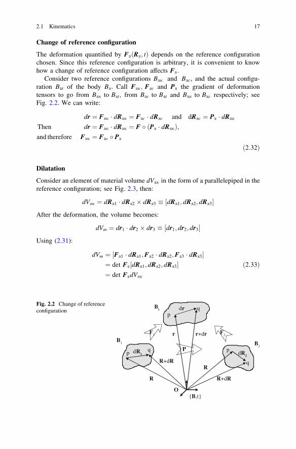
Consider two reference configurations Baj and Bac, and the actual configu-ration Bat of the body Ba. Call Faj; Fac and Pa the gradient of deformationtensors to go from Baj to Bat; from Bac to Bat and Baj to Bac respectively; seeFig. 2.2. We can write:

dr ¼ Faj � dRaj ¼ Fac � dRac and dRac ¼ Pa � dRaj

Then dr ¼ Faj � dRaj ¼ F � Pa � dRajð Þ;and therefore Faj ¼ Fac � Pa

ð2:32Þ

Dilatation

Consider an element of material volume dVaj in the form of a parallelepiped in thereference configuration; see Fig. 2.3, then:

dVaj ¼ dRa1 � dRa2 � dRa3 � dRa1; dRa2; dRa3½

After the deformation, the volume becomes:

dVm ¼ dr1 � dr2 � dr3 � dr1; dr2; dr3½

Using (2.31):

dVm ¼ Fa1 � dRa1;Fa2 � dRa2;Fa3 � dRa3½ ¼ det Fa dRa1; dRa2; dRa3½ ¼ det FadVaj

ð2:33Þ

p

q

B1

dR1

drp

q

Bt

RR+dR

r+drr

O{B,t}

p

q

dR2

B2

R+dRR

P

F1 F

2

Fig. 2.2 Change of referenceconfiguration

2.1 Kinematics 17

Then,

U2a ¼ FT

a � Fa ¼ Ca and V2a ¼ Fa � F2

a ¼ Ba ð2:37Þ

Since Ua and Va are symmetric and positive definite tensors and Qa is anorthogonal tensor, it can be shown that the characteristic values of Ua and Va arethe same:

Ua ¼Xn

a¼1

kkukuk and Va ¼Xn

a¼1

kkvkvk ð2:38Þ

and that the characteristic vectors are related by de rotation:

vk ¼ Qa � uk ð2:39Þ

Velocity and acceleration

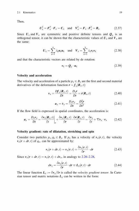
The velocity and acceleration of a particle pa 2 Ba are the first and second materialderivatives of the deformation function r ¼ f a Ra; tð Þ:

va ¼Df a Ra; tð Þ

Dt¼ Dar

Dt¼ _r Ra; tð Þ ð2:40Þ

aa ¼ _va ¼Dava

Dt¼ D2

ar

Dt2ð2:41Þ

If the flow field is expressed in spatial coordinates, the acceleration is:

aa ¼Dava

Dt¼ ova Ra; tð Þ

ot

��r

þ ova Ra; tð Þor

� or Ra; tð Þot

¼ ova

otþrva � va ð2:42Þ

Velocity gradient: rate of dilatation, stretching and spin

Consider two particles pa; qa 2 Ba. If pa has a velocity of va r; tð Þ, the velocityva rþ dr; tð Þ of qa; can be approximated by:

va rþ dr; tð Þ ¼ vaðr; tÞ þovaðr; tÞ

or� dr ð2:43Þ

Since va rþ dr; tð Þ ¼ vaðr; tÞ þ dva, in analogy to 2.26–2.28,

dva ¼ovaðr; tÞ

or� dr � La r; tð Þ � dr ð2:44Þ

The linear function La :¼ ova=or is called the velocity gradient tensor. In Carte-sian tensor and matrix notations La can be written in the form:

2.1 Kinematics 19

La ¼ rva ¼ovai

oxjeiej ¼ BT

ova1

ox1

ova1

ox2

ova1

ox3ova2

ox1

ova2

ox2

ova2

ox3ova3

ox1

ova3

ox2

ova3

ox3

2666664

3777775

B ð2:45Þ

The relationship between La and Fa can be obtained by calculating _va ¼ d _r fromEq. (2.31):

d _v ¼ d _r ¼ D

DtFa � dRað Þ

¼ _Fa � dRa ¼ _Fa � F�1a dr

¼ La � dr

Therefore:

La ¼ _FaF�1a ð2:46Þ

The velocity gradient can be separated into three irreducible parts, which aremutually orthogonal:

La ¼13

tr Lað ÞIRateofexpansion

orrateofdilatationtensor:

þ 12

La þ LTa

� �� 1

3tr Lað ÞI

� �

Rateofsheartensororstrechingtensor:

þ 12

La � LTa

� �

Rateofrotationtensororspintensor:

ð2:47Þ

To show that tr La represents the rate of dilatation, calculate the following:

tr La ¼ trrva ¼ovai

oxi

¼ r � va

On the other hand, take de derivative of the dilatation J r; tð Þ:

_Ja ¼D

Dtdet Fað Þ

¼ det Fatr _FaF�1a

� �

¼ det Fatr La

ð2:48Þ

From (2.48) we can write:

tr La ¼ r � va ¼_J

Jð2:49Þ


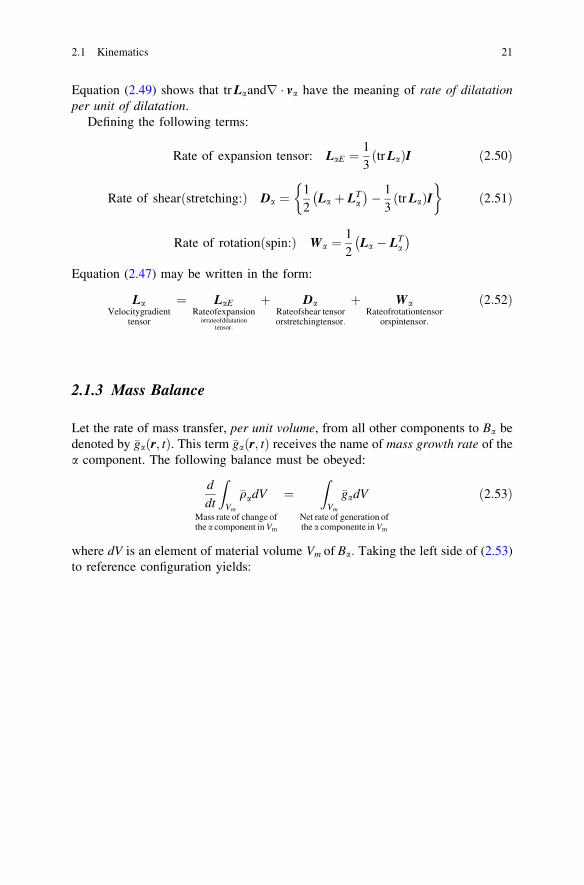
Equation (2.49) shows that tr Laandr � va have the meaning of rate of dilatationper unit of dilatation.

Defining the following terms:

Rate of expansion tensor: LaE ¼13

tr Lað ÞI ð2:50Þ

Rate of shear stretching:ð Þ Da ¼12

La þ LTa

� �� 1

3tr Lað ÞI

� �ð2:51Þ

Rate of rotation spin:ð Þ Wa ¼12

La � LTa

� �

Equation (2.47) may be written in the form:

LaVelocitygradient

tensor

¼ LaERateofexpansion

orrateofdilatationtensor:

þ DaRateofshear tensororstretchingtensor:

þ WaRateofrotationtensor

orspintensor:

ð2:52Þ

2.1.3 Mass Balance

Let the rate of mass transfer, per unit volume, from all other components to Ba bedenoted by �gaðr; tÞ. This term �gaðr; tÞ receives the name of mass growth rate of thea component. The following balance must be obeyed:

d

dt

Z

Vm

�qadV

Mass rate of change ofthe a component in Vm

¼Z

Vm

�gadV

Net rate of generation ofthe a componente in Vm

ð2:53Þ

where dV is an element of material volume Vm of Ba: Taking the left side of (2.53)to reference configuration yields:

2.1 Kinematics 21

d

dt

Z

Vm

�qadV ¼Z

Vj

D

Dt�qaJað ÞdV

¼Z

Vj

_�qaJa þ �qa_Ja

� �dV

¼Z

Vj

_�qa þ �qar � va� �

JadV

¼Z

Vm

o�qa

otþr � �qava

� �dV

¼Z

Vm

o�qa

otdV þ

Z

Vm

r � �qavadV

¼Z

Vm

o�qa

otdV þ

I

Sm

�qava � ndV

ð2:54Þ

Substituting in (2.53) gives a new form of the mass balance of Ba:Z

Vm

o�qa

otdV þ

I

Sm

�qa va � nð ÞdV ¼Z

Vm

�gadV ð2:55Þ

On the other hand, both volume integrals in (2.53) maybe taken to the referenceconfiguration to obtain:

Z

Vj

D

Dt�qaJað Þ � �gaJa

� �dV ¼ 0 ð2:56Þ

Performing the material derivative:Z

Vj

_�qaJa þ �qa_Ja � �gaJa

� �dV ¼ 0

Z

Vj

_�qaJa þ �qar � vaJa � �gaJa� �

dV ¼ 0

Z

Vj

_�qa þ �qar � va � �ga� �

JadV ¼ 0

Z

Vm

_�qa þ �qar � va � �ga� �

dV ¼ 0

Using the localization theorem (Gurtin 1981) yields:

_�qa þ �qar � va ¼ �ga ð2:57Þ

Writing the material derivative in terms of the spatial derivative and combining theresult with the second term of Eq. (2.57) gives:

o�qa

otþr � �qava ¼ �ga ð2:58Þ


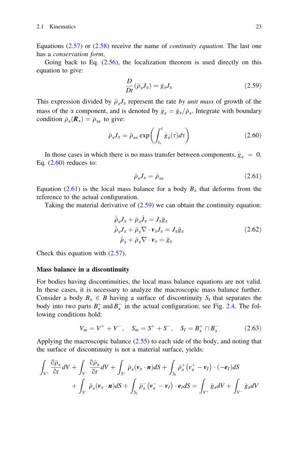
Equations (2.57) or (2.58) receive the name of continuity equation. The last onehas a conservation form.

Going back to Eq. (2.56), the localization theorem is used directly on thisequation to give:

D

Dt�qaJað Þ ¼ �gaJa ð2:59Þ

This expression divided by �qaJa represent the rate by unit mass of growth of the

mass of the a component, and is denoted by g_

a ¼ �ga=�qa. Integrate with boundarycondition �qa Rað Þ ¼ �qaj to give:

�qaJa ¼ �qaj exp

Z t

tj

g_

aðsÞds

� �ð2:60Þ

In those cases in which there is no mass transfer between components, g_

a ¼ 0;Eq. (2.60) reduces to:

�qaJa ¼ �qaj ð2:61Þ

Equation (2.61) is the local mass balance for a body Ba that deforms from thereference to the actual configuration.

Taking the material derivative of (2.59) we can obtain the continuity equation:

_�qaJa þ �qa_Ja ¼ Ja�ga

_�qaJa þ �qar � vaJa ¼ Ja�ga

_�qa þ �qar � va ¼ �ga

ð2:62Þ

Check this equation with (2.57).

Mass balance in a discontinuity

For bodies having discontinuities, the local mass balance equations are not valid.In these cases, it is necessary to analyze the macroscopic mass balance further.Consider a body Ba 2 B having a surface of discontinuity SI that separates thebody into two parts Bþa and B�a in the actual configuration; see Fig. 2.4. The fol-lowing conditions hold:

Vm ¼ Vþ þ V�; Sm ¼ Sþ þ S�; SI ¼ Bþa \ B�a ð2:63Þ

Applying the macroscopic balance (2.55) to each side of the body, and noting thatthe surface of discontinuity is not a material surface, yields:Z

Vþ

o�qa

otdV þ

Z

V�

o�qa

otdV þ

Z

Sþ�qa va � nð ÞdSþ

Z

SI

�qþa vþa � vI

� �� ð�eIÞdS

þZ

S��qa va � nð ÞdSþ

Z

SI

�q�a v�a � vI

� �� eIdS ¼

Z

Vþ�gadV þ

Z

V��gadV

2.1 Kinematics 23

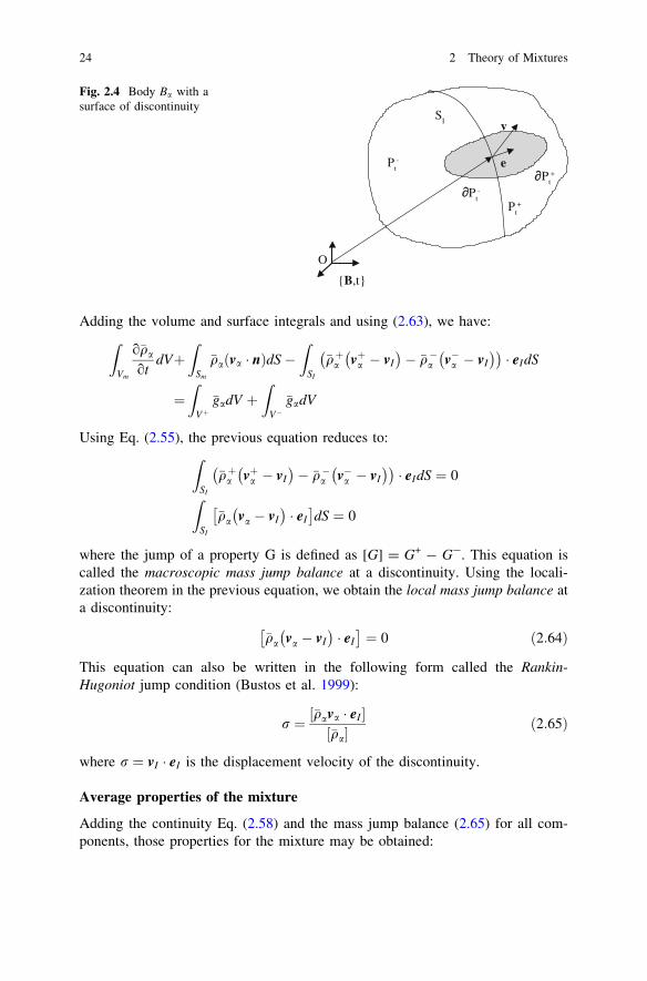
Adding the volume and surface integrals and using (2.63), we have:Z

Vm

o�qa

otdVþ

Z

Sm

�qa va � nð ÞdS�Z

SI

�qþa vþa � vI

� �� q�a v�a � vI

� �� eIdS

¼Z

Vþ�gadV þ

Z

V��gadV

Using Eq. (2.55), the previous equation reduces to:Z

SI

�qþa vþa � vI

� �� q�a v�a � vI

� �� eIdS ¼ 0

Z

SI

�qa va � vI

� �� eI

dS ¼ 0

where the jump of a property G is defined as [G] = G+ - G-. This equation iscalled the macroscopic mass jump balance at a discontinuity. Using the locali-zation theorem in the previous equation, we obtain the local mass jump balance ata discontinuity:

�qa va � vI

� �� eI

¼ 0 ð2:64Þ

This equation can also be written in the following form called the Rankin-Hugoniot jump condition (Bustos et al. 1999):

r ¼ �qava � eI½ �qa½

ð2:65Þ

where r ¼ vI � eI is the displacement velocity of the discontinuity.

Average properties of the mixture

Adding the continuity Eq. (2.58) and the mass jump balance (2.65) for all com-ponents, those properties for the mixture may be obtained:

O

{B,t}

SI

Pt+

Pt-

Pt-

Pt+

e

v

Fig. 2.4 Body Ba with asurface of discontinuity


o

ot

Xn

a¼1

�qa

!þr �

Xn

a¼1

�qava ¼Xn

a¼1

�ga ð2:66Þ

r ¼

Pn

a¼1�qava � eI

� �

Pn

a¼1�qa

� � ð2:67Þ

According to the initial postulates, the mixture should follow the laws of a purematerial; therefore, the continuity equation and the mass jump condition for themixture should be:

oqotþr � qv ¼ 0 ð2:68Þ

r ¼ qv � eI½ q½ ð2:69Þ

where q and v are the mass density and mass average or convective velocity of themixture. Comparing Eqs. (2.66) and (2.67) with (2.68) and (2.69) respectively, wededuce the following definitions for the mixture properties:

Mass density q ¼Xn

a¼�qa ð2:70Þ

Mass average velocity v ¼

Pn

a¼1�qava

Pn

a¼1�qa

¼

Pn

a¼1�qava

qð2:71Þ

Mass growth rateXn

a¼1

�ga ¼ 0 ð2:72Þ

This last equation indicates that no net production of mass occurs.

Convective diffusion equation

Sometimes it is convenient to express the continuity equation of each componentin terms of the convective mass flux density jaC ¼ �qav of that component. Addingand subtracting the convective flux per unit volume r � �qav, yields:

o�qa

otþr � �qav ¼ �r � �qa va � vð Þ þ �ga

Defining the diffusive flux density by jaD :¼ �qa va � vð Þ ¼ �qaua, where ua ¼va � v is the diffusion velocity, we can write:

2.1 Kinematics 25

o�qa

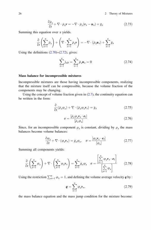
otþr � �qav ¼ �r � �qa va � uað Þ þ �ga ð2:73Þ

Summing this equation over a yields.

o

ot

Xn

a¼1

�qa

!þ r �

Xn

a¼1

�qav

!¼ �r � �qauað Þ þ

Xn

a¼1

�ga

Using the definitions (2.70)–(2.72), gives:

Xn

a¼1

jaD ¼Xn

a¼1

�qaua ¼ 0 ð2:74Þ

Mass balance for incompressible mixtures

Incompressible mixtures are those having incompressible components, realizingthat the mixture itself can be compressible, because the volume fraction of thecomponents may be changing.

Using the concept of volume fraction given in (2.7), the continuity equation canbe written in the form:

o

ot�qauað Þ þ r � �qauavað Þ ¼ �ga ð2:75Þ

r ¼ �qauava � eI½ �qaua½ ð2:76Þ

Since, for an incompressible component qa is constant, dividing by qa the massbalances become volume balances:

oua

otþr � uavað Þ ¼ g

_

aua; r ¼ uava � eI½ ua½

ð2:77Þ

Summing all components yields:

o

ot

Xn

a¼1

ua

!þr �

Xn

a¼1

uava

!¼Xn

a¼1

g_

aua r ¼

Pn

a¼1uava � eI

� �

Pn

a¼1ua

� � ð2:78Þ

Using the restrictionPn

a¼1 ua ¼ 1; and defining the volume average velocity q by :

q ¼Xn

a¼1

uava; ð2:79Þ

the mass balance equation and the mass jump condition for the mixture become:


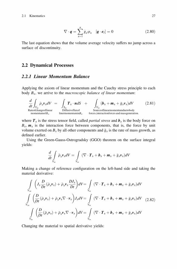
r � q ¼Xn

a¼1

g_

aua q � eI½ ¼ 0 ð2:80Þ

The last equation shows that the volume average velocity suffers no jump across asurface of discontinuity.

2.2 Dynamical Processes

2.2.1 Linear Momentum Balance

Applying the axiom of linear momentum and the Cauchy stress principle to eachbody Ba; we arrive to the macroscopic balance of linear momentum:

d

dt

Z

Vm

�qavadV

RateofchangeoflinearmomentumofBa:

¼Z

Sm

Ta � ndS

DiffusivefluxoflinermomentuminBa:

þZ

Vm

ba þma þ �gavað ÞdV

Sourceoflinearmomentumduetobodyforces;interactionforces and massgeneration:

ð2:81Þ

where Ta is the stress tensor field, called partial stress and ba is the body force onBa; ma is the interaction force between components, that is, the force by unitvolume exerted on Ba by all other components and �ga is the rate of mass growth, asdefined earlier.

Using the Green-Gauss-Ostrogradsky (GGO) theorem on the surface integralyields:

d

dt

Z

Vm

�qavadV ¼Z

Vm

r � Ta þ ba þma þ �gavað ÞdV

Making a change of reference configuration on the left-hand side and taking thematerial derivative:

Z

Vaj

JaD

Dt�qavað Þ þ �qava

DJa

Dt

� �dV¼

Z

Vm


Z

Vaj

D

Dt�qavað Þ þ �qavar � va

� �JadV¼

Z

Vm


Z

Vm

D


� �dV¼

Z

Vm


ð2:82Þ

Changing the material to spatial derivative yields:

2.1 Kinematics 27

Z

Vm

o

ot�qavað Þ þ �qava � rva þ �qavar � va

� �dV ¼

Z

Vm


Z

Vm

o

ot�qavað Þ þ r � �qavavað Þ

� �dV ¼

Z

Vm


Z

Vm

o

ot�qavað Þ þ r � �qavavað Þ � r � Ta � ba �ma � �gava

� �dV ¼ 0

ð2:83Þ

Using the localization theorem (Gurtin 1981) leads to the linear momentum bal-ance in the conservation form:

o

ot�qavað Þ þ r � �qavavað Þ ¼ r � Ta þ ba þma þ �gava ð2:84Þ

If instead we take the derivative of (2.82) in the following form:Z

Vm

D


� �dV ¼

Z

Vm


Z

Vm

_�qava þ �qa_va þ �qavar � va �r � Ta � ba �ma � �gava

� �dV ¼ 0

Z

Vm

_�qa þ �qar � va � �ga� �|fflfflfflfflfflfflfflfflfflfflfflfflfflfflfflfflffl{zfflfflfflfflfflfflfflfflfflfflfflfflfflfflfflfflffl}

by continuity equation¼ 0

va þ �qa_va þ�r � Ta � ba �ma

0B@

1CAdV ¼ 0

Z

Vm

�qa_va þ�r � Ta � ba �mað ÞdV ¼ 0 ;

and using the localization theorem:

�qa _va ¼ r � Ta þ ba þma ð2:85Þ

Linear momentum jump balance

In regions having discontinuities, Eqs. (2.84) and (2.85) are still valid on each sideof the discontinuity, but they are not valid at the discontinuity. Following a pro-cedure similar to that used previously for the mass jump balance, we write the lastequation of (2.83) in the form:


Z

Vm

o

ot�qavað Þ � ba �ma � �gava

� �dV ¼ �

Z

Vm

r � �qavavað Þ � r � Tað ÞdV

Z

Vm

o


� �dV ¼ �

I

Sm

�qava va � nð ÞdS�I

Sm

Ta � ndS

Applying this equation to each side of the discontinuity yields:Z

Vþ

o


� �dV þ

Z

V�

o�qavað Þ � ba �ma � �gava

� �dV

�x ¼�I

Sþ

�qava va � nð ÞdS�Z

SI

�qþa vþa vþa � vI

� �� eIð ÞdS�

I

S�

�qava va � nð ÞdS

�I

SI

�q�a v�a v�a � vI

� �� eIdS�

I

Sþ

Ta � ndS�Z

SI

Tþa � ð�eIÞdS�I

S�

Ta � ndS

�Z

SI

T�a � eIdS

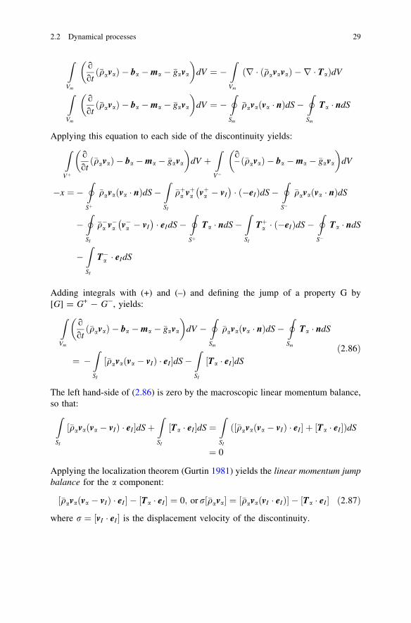
Adding integrals with (+) and (–) and defining the jump of a property G by[G] = G+ - G-, yields:Z

Vm

o


� �dV �

I

Sm

�qava va � nð ÞdS�I

Sm

Ta � ndS

¼ �Z

SI

�qava va � vIð Þ � eI½ dS�Z

SI

Ta � eI½ dSð2:86Þ

The left hand-side of (2.86) is zero by the macroscopic linear momentum balance,so that:Z

SI

�qava va � vIð Þ � eI½ dSþZ

SI

Ta � eI½ dS ¼Z

SI

�qava va � vIð Þ � eI½ þ Ta � eI½ ð ÞdS

¼ 0

Applying the localization theorem (Gurtin 1981) yields the linear momentum jumpbalance for the a component:

�qava va � vIð Þ � eI½ � Ta � eI½ ¼ 0; or r �qava½ ¼ �qava vI � eIð Þ½ � Ta � eI½ ð2:87Þ

where r ¼ vI � eI½ is the displacement velocity of the discontinuity.

2.2 Dynamical processes 29

Linear momentum balance for a mixtureSumming Eq. (2.84) for all component results in:

o

ot

Xn

a¼1

�qavað Þ þ r �Xn

a¼1

�qavavað Þ ¼ r �Xn

a¼1

Ta þXn

a¼1

ba þma þ �gavað Þ

Substituting the component velocity by the diffusion velocity by means of equationua ¼ va � v in the second term of the left-hands side yields:

o

ot

Xn

a¼1

�qavað Þþr �Xn

a¼1

�qa ua þ vð Þ ua þ vð Þð Þ ¼ r �Xn

a¼1

Ta þXn

a¼1


o

ot

Xn

a¼1

�qavað Þþr �Xn

a¼1

�qauavð Þ þ r �Xn

a¼1

�qavuað Þ þ r �Xn

a¼1

�qavvð Þ

¼ r �Xn

a¼1

Ta�r �Xn

a¼1

�qauauað Þ þXn

a¼1


Using the definitions (2.70)–(2.72) we get:

oqotþr � qvvð Þ ¼ r �

Xn

a¼1

Ta �Xn

a¼1

�qauauað Þ !

þXn

a¼1


For the mixture the linear momentum of a single component should be valid, then:

oqotþr � qvv ¼ r � T þ b

Comparing the last two equations we conclude that it is necessary that:

T ¼ TI �Xn

a¼1

�qauaua; b ¼Xn

a¼1

ba;Xn

a¼1

ma þ �gavð Þ ¼ 0 ð2:88Þ

with TI ¼Xn

a¼1

Ta ð2:89Þ

The term TI receives the name of the internal part of the stress tensor (Truesdell1984). The last term in (2.88) indicates that no net production of linear momentumexists, and that the growth in one component is done at the expense of the linearmomentum of the other components.

2.2.2 Angular Momentum Balance

The application of Euler’s second law for the angular momentum and Cauchy’sstress principle to the a component of the body gives the macroscopic angularmomentum balance:


d

dt

Z

Vm

r� rq

� �� qava

� �dV ¼

Z

Sm

r� rq

� �� Ta � n

� �dS

þZ

Vm

r� rq

� �� ba þma þ �gavað Þ

� �dSþ

Z

Vm

aaqdV

ð2:90Þ

where rq is the position of a fixed point Q with respect to which the torques andangular momentum are calculated.

When the field variables are smooth and continuous, a procedure similar to thatused in the previous section leads to the local angular momentum balance:

Ta � TTa ¼ Aaq ð2:91Þ

where Aaq is the skew tensor corresponding to the axial vector �aaq. If we assumethat there is no interchange of angular momentum between components, �aaq ¼ 0and the stress tensors for the components are symmetric:

Ta ¼ TTa : ð2:92Þ

2.2.3 Dynamic Process

Consider a mixture B formed by component Ba � B; with a ¼ 1; 2; . . .; n: Wesay that the following field variables r ¼ f a Ra; tð Þ, �qa ¼ �qa r; tð Þ, Ta ¼ Ta r; tð Þ,ba ¼ ba r; tð Þ, �ga ¼ �ga r; tð Þ and ma ¼ ma r; tð Þ, constitute a dynamic process if theyobey the following field equations in regions where they are smooth andcontinuous:

o�qa

otþr �qavað Þ ¼ �ga ð2:93Þ

o

ot�qavað Þ þ r � �qavavað Þ ¼ r � Ta þma þ �qava ð2:94Þ

and the following jump balance at discontinuities:

r �qa½ ¼ �qava � eI½ ; r �qava � eI½ ¼ �qavava � eI½ � Ta � eI½ ð2:95Þ

For this dynamic process to be complete, constitutive equations relating thekinematical with the dynamical variables must be postulated: Ta; rð Þ, ba; rð Þ,ma; rð Þ and �ga; rð Þ. A dynamic process for these six field variables

r; �qa; Ta; ba and �ga is admissible when the six equations are satisfied.

2.2 Dynamical processes 31

References

Atkin, R. J., & Crain, R. E. (1976). Continuum theories of mixtures: Basic theory and historicaldevelopment. The Quarterly Journal of Mechanics and Applied Mathematics, 29, 209–244.

Bedford, A., & Drumheller, D. S. (1983). Theories of immiscible and structured mixtures.International Journal of Engineering Science, 21(8), 863–960.

Bowen, R. M. (1976). Theory of mixtures. In A. C. Eringen (Ed.), Continuum physics (Vol. III).Waltham: Academic Press.

Bustos, M. C., Concha, F., Bürger, R., & Tory, E. M. (1999). Sedimentation and thickening,phenomenological foundation and mathematical theory. Dordrecht: Kluwer AcademicPublications.

Concha, F., & Barrientos, A. (1993). Mecánica Racional Moderna, Termomecánica del MedioContinuo (Vol. 2, pp. 248–266). Dirección de Docencia, Universidad de Concepción.

Concha, F., (2001). Manual de Filtración y Separación, CIC-Red Cettec, CETTEM Ltda., EdmundoLarenas 270 Concepción, Chile.

Drew, D. A. (1983). Mathematical modeling of two-phase flow. Annual Review of FluidMechanics, 15, 261–291.

Drew, A. D., & Passman, S.L. (1998). Theory of multicomponent fluids. Berlin: Springer.Gurtin, M. E. (1981). An Introduction. Academic Press, New York to Continuum Mechanic.Rajagopal, K. R., & Tao, L. (1995). Mechanics of mixtures, Worlds Scientific, Singapore.Truesdell, C., & Toupin, R. A. (1960). The classical field theories of mechanics. In S. Flügge

(Ed.), Handbook of physics (Vol. III–1). New York: Springer.Truesdell, C. (1965). Sulle basi de la termomecanica, Rend. Acad. Lincei, 22, 33–88, 1957.

Traducción al inglés en: Rational Mechanics of Materials, Int. Sci. Rev. Ser. 292–305, Gordon& Breach, New York.

Truesdell, C. (1984). Rational thermodynamics (2nd ed.). New York: Springer.Ungsrish, M. (1993). Hydrodynamics of suspensions. Berlin: Springer.


http://www.springer.com/978-3-319-02483-7

Documents

Theory of Mixtures