Embed Size (px)
Citation preview

PHYSICAL REVIEW E 95, 033303 (2017)
Theory of linear sweep voltammetry with diffuse charge: Unsupported electrolytes,thin films, and leaky membranes
David Yan,1,* Martin Z. Bazant,2 P. M. Biesheuvel,3 Mary C. Pugh,4 and Francis P. Dawson1
1Department of Electrical and Computer Engineering, University of Toronto, Toronto, Ontario, Canada M5S 3G42Department of Chemical Engineering and Department of Mathematics, Massachusetts Institute of Technology,
Cambridge, Massachusetts 02139, USA3Wetsus, European Centre of Excellence for Sustainable Water Technology, The Netherlands
4Department of Mathematics, University of Toronto, Toronto, Ontario, Canada M5S 2E4(Received 31 October 2016; revised manuscript received 11 January 2017; published 8 March 2017)
Linear sweep and cyclic voltammetry techniques are important tools for electrochemists and have a varietyof applications in engineering. Voltammetry has classically been treated with the Randles-Sevcik equation,which assumes an electroneutral supported electrolyte. In this paper, we provide a comprehensive mathematicaltheory of voltammetry in electrochemical cells with unsupported electrolytes and for other situations wherediffuse charge effects play a role, and present analytical and simulated solutions of the time-dependent Poisson-Nernst-Planck equations with generalized Frumkin-Butler-Volmer boundary conditions for a 1:1 electrolyteand a simple reaction. Using these solutions, we construct theoretical and simulated current-voltage curvesfor liquid and solid thin films, membranes with fixed background charge, and cells with blocking electrodes.The full range of dimensionless parameters is considered, including the dimensionless Debye screening length(scaled to the electrode separation), Damkohler number (ratio of characteristic diffusion and reaction times),and dimensionless sweep rate (scaled to the thermal voltage per diffusion time). The analysis focuses on thecoupling of Faradaic reactions and diffuse charge dynamics, although capacitive charging of the electricaldouble layers is also studied, for early time transients at reactive electrodes and for nonreactive blockingelectrodes. Our work highlights cases where diffuse charge effects are important in the context of voltammetry, andillustrates which regimes can be approximated using simple analytical expressions and which require more carefulconsideration.
DOI: 10.1103/PhysRevE.95.033303
I. INTRODUCTION
Polarography or linear sweep voltammetry (LSV) orcyclic voltammetry (CV) is the most common method ofelectroanalytical chemistry [1–3], pioneered by Heyrovskyand honored by a Nobel Prize in Chemistry in 1959. Theclassical Randles-Sevcik theory of polarograms is based onthe assumption of diffusion limitation of the active speciesin a neutral liquid electrolyte, driven by fast reactions at theworking electrode [4–6]. Extensions for slow Butler-Volmerkinetics (or other reaction models) are also available [1]. Thehalf-cell voltage is measured at a well-separated referenceelectrode in the bulk liquid electrolyte, which is assumed to beelectroneutral, based on the use of a supporting electrolyte [7].
Most classical voltammetry experiments and models fea-tured a supported electrolyte: an electrolyte with an inertsalt added to remove the effect of electromigration. Inmany electrochemical systems of current interest, however,the electrolyte is unsupported, doped, or strongly confinedby electrodes with nanoscale dimensions. Examples includesupercapacitors, [8], capacitive deionization [9], pseudocapac-itive deionization and energy storage [10,11], electrochemicalthin films [12–15], solid electrolytes used in Li-ion or Li-metal[16,17], electrochemical breakdown of integrated circuits [18],fuel cells [19,20], nanofludic systems [21–23], electrodialysis[24–26], and charged porous “leaky membranes” [27,28]
for shock electrodialysis [29,30] and shock electrodeposition[31,32]. In all of these situations, diffuse ionic charge mustplay an important role in voltammetry, which remains to befully understood.
Despite an extensive theoretical and experimental literatureon this subject (reviewed below), to the authors’ knowledge,there has been no comprehensive mathematical modeling ofthe effects of diffuse charge on polarograms, while fully takinginto account time-dependent electromigration and Frumkineffects of diffuse charge on Faradaic reaction rates. The goalof this work is thus to construct and solve a general model forvoltammetry for charged electrolytes. We consider the simplestPoisson-Nernst-Planck (PNP) equations for ion transport fordilute liquid and solid electrolytes and leaky membranes,coupled with “generalized” Frumkin-Butler-Volmer (FBV)kinetics for Faradaic reactions at the electrodes [12,33–37],as reviewed by Biesheuvel, Soestbergen, and Bazant [14]and extended in subsequent work [10,11,15]. Unlike mostprior analyses, however, we make no assumptions about theelectrical double layer (EDL) thickness, Stern layer thickness,sweep rate, or reaction rates in numerical solutions of thefull PNP-FBV model. We also define a complete set ofdimensionless parameters and take various physically relevantlimits to obtain analytical results whenever possible, which arecompared with numerical solutions in the appropriate limits.
The paper is structured as follows. We begin with a review oftheoretical and experimental studies of diffuse-charge effectsin voltammetry in Sec. II. The PNP-FBV model equationsare formulated and cast in dimensionless form in Sec. III,
2470-0045/2017/95(3)/033303(20) 033303-1 ©2017 American Physical Society
YAN, BAZANT, BIESHEUVEL, PUGH, AND DAWSON PHYSICAL REVIEW E 95, 033303 (2017)
followed by voltammetry simulations on a single electrode ina supported and unsupported electrolyte in Sec. IV. Section Vshows simulations on liquid and solid electrochemical thinfilms, considering both the thin and thick double layer limits.In Sec. VI, we simulate ramped voltages applied to porous“leaky” membranes with fixed background charge. Finally,ramped voltages are applied to systems with one or twoblocking electrodes in Sec. VII, and simulation results arecompared with theoretical capacitance curves. We concludewith a summary and outlook for future work.
II. HISTORICAL REVIEW
The modeling of diffuse charge dynamics in electro-chemical systems has a long history, reviewed by Bazant,Thornton, and Ajdari [38]. Frumkin [39] and Levich [40]are credited with identifying the need to consider effects ofdiffuse charge on Butler-Volmer reaction kinetics at electrodesin unsupported electrolytes by pointing out that the potentialdrop which drives reactions is across the Stern layer ratherthan in relation to a reference electrode far away, althoughcomplete mathematical models for dynamical situations werenot formulated until much later. In electrochemical impedancespectroscopy (EIS) [41], it is well known that the double-layercapacitance must be considered in parallel with the Faradaic re-action resistance in order to describe the interfacial impedanceof electrodes. Since the pioneering work of Jaffe [42,43] forsemiconductors and Chang and Jaffe for electrolytes [44],Macdonald [45,46] and others have formulated microscopicPNP-based models using the Chang-Jaffe boundary conditions[47], which postulate mass-action kinetics, proportional to theactive ion concentration at the surface. This approximationincludes the first “Frumkin correction,” i.e., the jump inactive species concentration across the diffuse layer, but notthe second, related to the jump in electric field that driveselectron transfer at the surface [12,14]. More importantly, allmodels used to interpret EIS measurements, whether basedon microscopic transport equations or macroscopic equivalentcircuit models, only hold for the small-signal response to aninfinitesimal sinusoidal applied voltage or current.
The nonlinear coupling of diffuse charge dynamics withFaradaic reaction kinetics has received far less attentionand, until recently, has been treated mostly by empiricalmacroscopic models, as reviewed by Biesheuvel, Soestbergen,and Bazant [14]. Examples of ad hoc approximations includefixing the electrode charge or zeta potential, independentlyfrom the applied current or voltage, and assuming a constantdouble layer capacitance in parallel with a variable Faradaicreaction resistance given by the Butler-Volmer equation. Suchempirical models are theoretically inconsistent, because theelectrode charge and double-layer capacitance are not constantindependent variables to be fitted to experimental data. Instead,the microscopic model must include a proper electrostaticboundary condition, relating surface charge to the jump inthe normal component of the Maxwell dielectric displacement[48], and the Butler-Volmer equation, or another reaction-ratemodel, must be applied at the same position (the “reactionplane”). This inevitably leads to nonlinear dependence of theelectrode surface charge on the local current density [10,12],which includes both Faradaic current from electron-transfer
reactions and Maxwell displacement current from capacitivecharging [35,38,49].
Interest in voltammetry in low conductivity solvents anddilute electrolytes with little to no supporting electrolyte hasslowly grown since the 1970s. Since the work of Buck [50], avariety of PNP-based microscopic models have been proposed[51–54], which provide somewhat different boundaryconditions than the FBV model described below. Since the1980s, various experiments have focused on the role ofsupporting electrolyte [2]. For example, Bond and co-workersperformed linear sweep [55] and cyclic [56,57] voltammetryusing the ferrocene oxidation reaction on a microelectrodewhile varying supporting electrolyte concentrations. One ofthe primary theoretical concerns at that time was modeling theextra Ohmic drop in the solution from the electromigrationeffects which entered into the physics due to low supportingelectrolyte concentration. Bond [58] and Oldham [59] bothsolved the PNP equations for steady-state voltammetry indilute solutions with either Nerstian or Butler-Volmer reactionkinetics to obtain expressions for the Ohmic drop. While theylisted the full PNP equations, they analytically solved thesystem only with the electroneutrality assumption or for smalldeviations from electroneutrality, which is a feature of manylater models as well [54,60,61]. The bulk electroneutralityapproximation is generally very accurate in macroscopicelectrochemical systems [7,62], although care must betaken to incorporate diffuse charge effects properly in theboundary conditions, as explained below. Bento, Thouin, andAmatore [63,64] continued this type of experimental work onvoltammetry and studied the effect of diffuse layer dynamicsand migrational effects in electrolytes with low support. Theyalso performed voltammetry experiments on microelectrodesin solutions while varying the ratio of supporting electrolyteto reactant, and noted shifts in the resulting voltammogramsand a change in the solution resistance [65].
More recently, Compton and co-workers have done exten-sive work involving theory [66–68], simulations [37,66,69,70](and see Chap. 7 of [3] or Chap. 10 of [2]), and experiments[71–74] on the effect of varying the concentration of thesupporting electrolyte on voltammetry. Besides consideringa different (hemispherical) electrode geometry motivated byultramicroelectrodes [75], there are two significant differencesbetween this body of work and ours, from a modelingperspective.
The first difference is that Compton and co-authors considerthree or more species in their models in order to account forthe supporting electrolyte and the effect of varying its concen-tration. The additional species in their work are sometimesneutral [71,72] and sometimes charged [66,70], dependingon the reaction being modeled. Modeling of uncharged andsupporting ionic species has also been a feature of other modelsin the literature [58–60]. In this work, we only consider the twoextremes: either an unsupported binary electrolyte or (briefly,for comparison) a fully supported electrolyte.
The second difference lies in their treatment of specificadsorption of ions and a related approximation used to simplifythe full model. Although some studies involve numericalsolutions of the full PNP equations with suitable electrostaticand reaction boundary conditions [37], many others employ the“zero-field approximation” for the thin double layers [37,69],
033303-2

THEORY OF LINEAR SWEEP VOLTAMMETRY WITH . . . PHYSICAL REVIEW E 95, 033303 (2017)
which is motivated by strong specific adsorption of ions. In thispicture, the Stern layer [76] (outside the continuum region ofion transport) is postulated to have two parts: an outer layer ofadsorbed ions that fully screens the surface charge, and an inneruncharged dielectric layer that represents solvent molecules onthe electrode surface. The assumption of complete screeningmotivates imposing a vanishing normal electric field as theboundary condition for the neutral bulk electrolyte at theelectrode outside the double layers. This assertion also hasthe effect of eliminating the electromigration term from theflux entering the double layers, despite the inclusion of thisterm in the bulk mass flux. Physically, this model assumesthat the electrode always remains close to the potential of zerocharge, even during the passage of transient large currents.
Here, we base our analysis on the PNP equations with“generalized FBV” boundary conditions [14,15], to describeFaradaic reactions at a working electrode, whose potentialis measured relative to the point of zero charge, in theabsence of specific adsorption of ions. The model postulates acharge-free Stern layer of constant capacitance, whose voltagedrop drives electron transfer according to the Butler-Volmerequation, where the exchange current is determined by thelocal concentration of active ions at the reaction plane. Thisapproach was first introduced by Frumkin and later applied byItskovich, Kornyshev, and Vorontyntsev [33,34] in the contextof solid electrolytes, with one mobile ionic species and fixedbackground charge. For general liquid or solid electrolytes,the FBV model based on the Stern boundary condition wasperhaps first formulated by Bazant and co-workers [12,14,35]and independently developed by He et al. [36] and Streeter andCompton [37]. The FBV-Stern model was extended to porouselectrodes and multicomponent electrolytes by Biesheuvel, Fu,and Bazant [10,11].
Most of the literature on modeling diffuse-charge effects inelectrochemical cells has focused on either linear ac response(impedance) or nonlinear steady-state response (differentialresistance), with a few notable exceptions. The PNP-FBVmodel was apparently first applied to chronoampereometry(response to a voltage step) by Streeter and Compton [37]and to chonopotentiometry (response to a current step) bySoestbergen, Biesheuvel, and Bazant [49], each in the limit ofthin double layers for unsupported binary liquid electrolytes.Here, we extend this work to voltammetry and consider a muchwider range of conditions, including thick double layers, fixedbackground charge, and slow reactions.
It is important to emphasize the generality of the PNP-FBV framework, which is not limited to thin double layersand stagnant neutral bulk electrolytes. Chu and Bazant [13]analyzed the model for a binary electrolyte under extremeconditions of overlimiting current, where the double layer losesits quasiequilibrium structure and expands into an extendedbulk space charge layer, and performed simulations of steadytransport across a thin film at currents over 25 times theclassical diffusion-limited current (which might be achieved insolid, ultrathin films). Transient space charge has also been an-alyzed in this way for large applied voltages, for both blockingelectrodes [38,77] and FBV reactions [49]. A validation of thePNP-FBV theory was recently achieved by Soestbergen [78],who fitted the model to experimental data of Lemay and co-workers for planar nanocavities [79,80]. The FBV model has
also been applied to nonlinear “induced-charge” electrokineticphenomena [81], in the asymptotic limit of thin double layers.Olesen, Bruus, and Ajdari [82,83] used the quasiequilibriumFBV double-layer model in a theory of ac electro-osmotic flowover microelectrode arrays. Moran and Posner [84] applied thesame approach to reaction-induced-charge electrophoresis ofreactive metal colloidal particles in electric fields [85].
Many of these recent studies have exploited effectiveboundary conditions for thin double layers, which weresystematically derived by asymptotic analysis and compared tofull solutions of the PNP equations, rather than ad hoc approx-imations. Matched asymptotic expansions were first appliedto steady-state PNP transport in the 1960s without consideringFBV reaction kinetics [86–89] and used extensively in theoriesof ion transport [24] and electro-osmotic fluid instabilities[90,91] in electrodialysis, involving ion-exchange membranesrather than electrodes. Baker and Verbrugge [92] analyzeda simplified problem with fast reactions, where the activespecies concentration vanishes at the electrode. Bazant andco-workers first used matched asymptotic expansions to treatFaradaic reactions using the PNP-FBV framework, applied tosteady conduction through electrochemical thin films [12,13].Richardson and King [93] extended this approach to deriveeffective boundary conditions for time-dependent problems,which provides rigorous justification for subsequent studiesof transient electrochemical response using the thin doublelayer approximation, including ours.
Finally, for completeness, we note that Moya et al. [94]recently analyzed a model of double-layer effects on LSVfor the case of a neutral electrolyte surrounding an ideal ion-exchange membrane with thin quasiequilibrium double layers,and no electrodes with Faradaic reactions to sustain the current.
III. MATHEMATICAL MODEL
A. Modeling domain
In this work, we consider ramped voltages applied toelectrochemical systems with one or two electrodes. Figure 1shows a sketch of both systems, with the directions of thevoltage and current density. The two electrode case models abattery or capacitor, whereas the one electrode case models anelectrode under test at the right-hand side of the domain withan ideal reservoir and potential set to zero at the left-hand side.
- +
+
+
+
+
+
+ ++ +
+
++
-
--
-
-
--
-
--
-
-
+-
(a) Single electrode
- +
++
+
+
+
+
++
+
+
++
-
-
---
--
--
-
--
(b) Two electrodes
FIG. 1. Diagram showing electrochemical systems with appliedvoltage V and resulting current J for a system with (a) a singleelectrode and (b) two electrodes. In the single-electrode case, theleft-hand boundary is modeled as an ideal reservoir with a fixedpotential. Also shown is a sketch of the potential inside the cell:dashed line is the potential in the bulk; solid line is the potential inthe diffuse region.
033303-3

YAN, BAZANT, BIESHEUVEL, PUGH, AND DAWSON PHYSICAL REVIEW E 95, 033303 (2017)
B. Poisson-Nernst-Planck equations for ion transport
Transport of ions in the bulk is described by a conservationequation for the concentration,
dCi
dτ= − ∂
∂XJNP,i , (1)
and the definition of the flux,
JNP,i = −Di
∂Ci
∂X− ziDiF
RTCi
∂�
∂X, (2)
where Ci(X,τ ) denotes the concentration of the ith speciesand zi is its associated charge number, where we take theconvention that the sign of the charge is attached to z (so thata negative ion has negative z). Di is the diffusivity of the ithspecies, and F , R, and T are Faraday’s constant, the ideal gasconstant, and temperature, respectively. Substituting Eq. (2)into Eq. (1) gives the time-dependent Nernst-Planck equationfor ions in the bulk [X ∈ (0,L)], where we replace the index i
with either + or − for the positive and negative ion:
∂C±∂τ
= ∂
∂X
[D±
∂C±∂X
+ z±D±F
RTC±
∂�
∂X
]. (3)
Note that this classical first approximation [34] neglectsexcluded volume (“crowding”) effects, which are importantin crystalline ionic solids [95] and ion insertion electrodes[96] especially at high voltages [81]. For solid electrolytesin a lattice, Bikerman’s model [97] can be used, and forliquid electrolytes there are hard sphere models such as theCarnahan-Starling model [98]. Without steric effects, themodel might be better for polymeric solid electrolytes withless severe volume constraints, or for doped solid crystals withlow carrier concentrations at sufficiently low voltages.
The potential �(X,τ ) is determined by Poisson’s equation,
−εs
∂2�
∂X2= F (z+C+ + z−C−), (4)
where εs is the bulk permittivity of the electrolyte. We will beconsidering 1:1 binary electrolytes in this work, and Eqs. (3)and (4) describe a system with two mobile charges. For a solidelectrolyte, negative ions take a fixed value of concentration,and so we set C−(X,τ ) = C0 and only solve one transportequation. For a “leaky membrane” [27], we add a constantbackground charge ρs to Eq. (4),
−εs
∂2�
∂X2= F (z+C+ + z−C− + ρs). (5)
Finally, for a supported electrolyte, we set �(X,τ ) = 0 andonly solve the two Nernst-Planck equations for each chargedspecies.
C. Frumkin-Butler-Volmer boundary conditions forFaradaic reactions
The boundary condition for Eq. (3) is given by
±(
D+∂C+∂X
+ z+DF
RT
∂�
∂X
)∣∣∣∣X=0,L
= JF (6)
for the flux of the cations, where the ± in Eq. (6) variesdepending on whether the boundary condition is applied atthe left or right boundary. We assume that the anion (C−) flux
is zero at both boundaries. For the Faradaic current JF , we usethe generalized Frumkin-Butler-Volmer (FBV) equation,
JF = Kc C+e( −αcnF��RT
) − Ka CM e( αanF��RT
). (7)
In particular, Eq. (7) models a reaction of the form
Cz++ + n e− � M, (8)
where n = z+ is the number of electrons transferred to reducethe cation to the metallic state M . An example of a reaction ofthe form (8) is the Cu-CuSO4 electrodeposition process, wherez+ = n = 2. Ka and Kc are the reaction rate parameters andαa,c is the so-called transfer coefficient, with αa + αc = 1. Inthe case of a blocking, or ideally polarizable electrode, or fora species which does not take part in the electrode reaction,Ka = Kc = 0. Following [15] and other models using FBVkinetics, �� is explicitly defined as being across the Sternlayer (and always as the potential at the electrode minus thepotential at the Stern plane), and the direction of JF is definedto be from the solution into the electrode.
The boundary condition on � at an electrode is
∓λs
∂�
∂X= ��, (9)
where again the sign ∓ is for the left-hand and right sideelectrode and λs is the effective width of the Stern layer,allowing for a different (typically lower) dielectric constant[12,35]. In this model, the point of zero charge (pzc) occurswhen �� = 0 across the Stern layer, so the potential of theworking electrode is defined relative to the pzc. For a moregeneral model with two electrodes having different pzc’s, anadditional potential shift must be added to Eq. (9) for at leastone electrode [36,37].
The system of equations is closed with a current conserva-tion equation [see Eq. (9) in [49]],
d�X(L,τ )
dτ= − 1
εs
{J (τ ) − FJF }, (10)
where J (τ ) can either be an externally set electrical currentor (when the voltage is prescribed as is the case in this work)a postprocessed electrical current, also defined to be from thesolution into the electrode. In Eq. (10), �X denotes the X
derivative of �.In this work, we will be using this model to consider the
effect of a ramped voltage at the right-hand side electrode. Theapplied voltage takes the form
V (τ ) = Sτ, (11)
where S is the voltage scan or sweep rate. For some simulationsin this work, we wish to model only one electrode, with theother approximating an ideal reference electrode or an idealreservoir. In this case, we use the electrode at X = L as theelectrode under test, and use the boundary conditions
C±(0,τ ) = C0, �(0) = 0 (12)
at X = 0, where C0 is a reference concentration.
D. Dimensionless equations
It is convenient to rescale the PNP equations so thatdistance, time, concentration, and potential are scaled to
033303-4

THEORY OF LINEAR SWEEP VOLTAMMETRY WITH . . . PHYSICAL REVIEW E 95, 033303 (2017)
interelectrode width, the diffusion time scale, a referenceconcentration, and the thermal voltage, respectively:
x ≡ X
L, t ≡ Dτ
L2, c± ≡ C±
C0, φ ≡ F�
RT. (13)
Rescaling the Poisson-Nernst-Planck equations (3) and (4)yields the dimensionless equations. For the remainder of thepaper, we will be assuming a 1:1 electrolyte (z+ = −z− = 1),equal diffusivities (D+ = D− = D), and restricting ourselvesto the electrode reaction in Eq. (8) with z+ = n = 1. Otherionic solutions and reactions can be modeled by making theappropriate changes to Eqs. (3), (4), and (7). The Nernst-Planck and Poisson equations become
∂c±∂t
= d
dx
[∂c±∂x
± c±∂φ
∂x
], (14)
−ε2 ∂2φ
∂x2= 1
2(c+ − c−), (15)
where ε = λD/L is the ratio between the Debye length λD ≡√εsRT
2F 2C0and L. To nondimensionalize the boundary conditions,
we introduce the following rescaled parameters:
kc = Kc L
4D, jr = Ka LCM
4DC0, δ = λs
λD
, (16)
so that Eq. (7) becomes (assuming αc = αa = 1/2)
±(
c+∂φ
∂x+ ∂c+
∂x
)∣∣∣∣x=0,1
= 4kc c+ e−�φ/2 − 4 jr e�φ/2.
(17)
Equation (9) rescales to
∓ε δ φx = �φ (18)
and finally Eq. (10) becomes
−ε2
2
d
dtφx(1,t) = j − [kc c+(1,t) e−�φ/2 − jr e�φ/2], (19)
where j is scaled to the limiting current density Jlim = 4FDC0L
.The rescaled equations contain two fundamental time
scales: the diffusion time scale, τD = L2/D, and the reactiontime scale, τR = L/K , for a characteristic reaction rate K .There is also the imposed voltage scan rate time scale,τS = RT
F/S. The ratios of these three time scales result in
two dimensionless groups: the nondimensional voltage scanrate,
S = τD
τS
= SL2F
DRT, (20)
and the nondimensional reaction rate,
k = τD
4τR
= KL
4D, (21)
also known as the “Damkohler number.” In Eq. (16), the lattertakes two forms, k = kc and k = jr , for the forward (oxidation)and backward (reduction) reactions with the characteristicrates, K = Kc and K = KaCM/C0, respectively.
The dimensionless model also contains thermodynamicinformation about the electrochemical reaction, independentof the overall reaction rate [1,10,96]. For any choice of a single
reaction-rate scaling, there is a third dimensionless group,which can be expressed as the (logarithm of) the ratio of thedimensionless forward and backward reaction rates,
lnkc
jr
= lnKcC0
KaCM
= �φ . (22)
This is the dimensionless equilibrium interfacial voltage,where the net Faradaic current [Eq. (17)] vanishes in detailedbalance between the oxidation and reduction reactions for thereactive cation at the bulk reference concentration C0.
E. Important limits
1. Supported electrolyte
As mentioned in Sec. II, we choose to model liquid elec-trolytes in the limit of high supporting salt concentrations bysetting φ(x,t) = 0 and removing Poisson’s equation [Eq. (15)]from the model. This has two effects: first, electromigration isno longer a part of the transport equations [Eq. (3)]. Second,the voltage difference �φ = v − φ(1) which enters into theFBV equation [Eq. (17)] is just the electrode potential sinceφ(1) = 0. This results in a time-dependent version of theclassical Randles-Sevcik system [1], with Butler-Volmer ratherthan Nernstian boundary conditions.
2. Thin double layers (electroneutral limit)
The dimensionless parameters ε and δ control how themodel handles the double layer and diffuse charge dynamics,respectively. The dimensionless Debye length ε governs theamount of charge separation that is allowed to occur, orequivalently the thickness of the diffuse layer relative todevice thickness. The parameter δ, which is effectively aratio of Stern and diffuse layer capacitance, controls thecompetition between the Stern and diffuse layers in overalldouble layer behavior. The electroneutral, or thin double layerlimit, corresponds to ε → 0. In this limit, Eq. (15) is simply
c+ = c−. (23)
Substituting Eq. (23) into the Nernst-Planck equations[Eq. (14)] results in the ambipolar diffusion equation for theconcentration c = c+ = c− (written here for equal diffusivi-ties),
∂c
∂t= ∂2c
∂x2(24)
and the following equation for the potential:
∂
∂x
(c∂φ
∂x
)= 0. (25)
In the limit of thin double layers, there are two furtherlimits on δ. The first is the “Gouy-Chapman” (GC) limit,δ → 0, which corresponds to a situation where all of thepotential drop in the double layer is across the diffuse region,and the second is the “Helmholtz” (H) limit, δ → ∞, whereall of the potential drop is across the Stern layer. In theformer case, the Boltzmann distribution for ions is invoked[c± = exp (∓�φD)] and Eq. (17) becomes
±(
c+∂φ
∂x+ ∂c+
∂x
)∣∣∣∣x=0,1
= 4kc c+ e−�φD − 4 jr , (26)
033303-5

YAN, BAZANT, BIESHEUVEL, PUGH, AND DAWSON PHYSICAL REVIEW E 95, 033303 (2017)
where �φD is the potential drop across the diffuse region. Inthe latter case, Eq. (17) becomes
±(
c+∂φ
∂x+ ∂c+
∂x
)∣∣∣∣x=0,1
= 4kc c+ e−�φS/2 − 4 jre�φS/2,
(27)where �φS is the potential drop across the Stern layer.
3. Fast reactions
The most common approximation for the boundary condi-tions in voltammetry is the Nernstian limit of fast reactions,kc,jr → ∞, for a fixed ratio, jr/kc, corresponding to a givenequilibrium half-cell potential for the reaction, Eq. (22). In thislimit, the left-hand sides of Eqs. (17) and (26),(27) approachzero, and all three boundary conditions reduce to the Nernstequation,
�φ = �φ + ln c+, (28)
where the bulk solution is used as the reference concentration.In order to place the Nernst equation in the standard form[1,96],
E = RT
nF�φeq = E + RT
nFln
C+Cref
, (29)
we must define the equilibrium interfacial voltage relative to astandard reference electrode (e.g., the standard hydrogen elec-trode in aqueous systems at room temperature and atmosphericpressure with Cref = 1 M) by shifting the reference potential,
E = RT
nF
(�φ − ln
C0
Cref
)= RT
nFln
KcCref
KaCM
. (30)
In this way, tables of standard half-cell potentials can beused to determine the ratio of reaction rate constants, andmeasurements of exchange current density can then determinethe individual oxidation and reduction rate constants.
IV. BULK LIQUID ELECTROLYTES
A. Model problem
The model problem for this section is a single electrodein an aqueous electrolyte with a reference electrode at x = 0and two mobile ions. Voltammetry on a single electrode insolution is one of the oldest problems in electrochemistry;experiments are usually conducted using the “three-electrodesetup,” where one electrode acts as a voltage reference whileanother (the counter electrode) provides current. Computa-tionally, this setup can be mimicked with Eq. (12) applied atX = 0. This models a cell with only one electrode, with theother approximating an ideal reference electrode or an idealreservoir.
In order to ensure that dynamics do not reach the referenceelectrode, we restrict ourselves to the regime S � 1 and t � 1.The reaction rate parameter k can either be fast (k � 1) or slow(k � 1), which corresponds to a diffusion-limited regime andreaction-limited regime, respectively.
B. Supported electrolytes
A supported electrolyte is where an inert salt is added (a saltwhich does not take part in electrode or bulk reactions) in order
to screen the electric field so as to render electromigrationeffects negligible (i.e., φ = 0 in the bulk). Voltammetrywith supported electrolytes has classically been treated as asemi-infinite diffusion problem. For an aqueous system at aplanar electrode with a reversible electrode reaction (reactionmuch faster than diffusion) involving two species denoted O(oxidized) and R (reduced), the current resulting from a slowramped voltage is given, using the present notation, by (seeChaps. 5 and 6 of [1])
J (τ ) = nFDO
(∂CO(X,τ )
∂X
)X=0
= nFAC∗O(πDOσ )
12 χ (στ ),
(31)
where σ ≡ nFS/RT (S is the scan rate) and χ is theRandles-Sevcik function. The same system of equations is alsooften considered for irreversible (slow reactions compared todiffusion) and “quasireversible” reactions, with the appropriatechanges to the boundary conditions.
The reaction we will be considering is
C+ + e− � M, (32)
where M represents the electrode material. Since the reactiononly involves one of the two ions as opposed to both asin the Randles-Sevcik case, the mathematics are simplifiedsomewhat and we are able to obtain an analytical solution. Thediffusion equation [Eq. (24)] needs to be solved on x ∈ (0,∞)with fast reactions [Eq. (28) with �φ = v(t)]. In order toprobe the forward, or reduction, reaction, we apply a voltage asv(t) = −St and compute the resulting current via j = ∂c
∂x|x=0.
These equations admit the solution
j (t) =√
Se−St erfi(√
St), (33)
where erfi(z) = 2√π
∫ z
0 exp x2 dx is the imaginary error func-tion. The derivation of Eq. (33) can be found in the Appendix.We term Eq. (33) a “modified” Randles-Sevcik equation,which applies to voltammetry on an electrode with fastreactions involving only one ionic species, and in a supportedelectrolyte. Figure 2 shows simulated j (t) curves with variousvalues of k compared to Eq. (33), with S = 50. The curvesin Fig. 2 exhibit the distinguishing features of single-reactionvoltammograms: current increases rapidly until most of thereactant at the electrode has been removed due to transportlimitation. The peak represents the competition between theincreasing rate of reaction and the decreasing amount ofreactant at the electrode. After the peak, the lack of reactantwins out, and there is a decrease in the amount of current theelectrode is able to sustain. Also worth noting is that at lowreaction rate k, the start of the voltammogram is exponentialrather than linear due to reaction limiting.
The simulated curves in Fig. 2 approach Eq. (33) in thelimit of large k, which makes Eq. (33) a good approximationfor the current response to a ramped voltage in a supportedelectrolyte with fast, single-species reaction. Note that due todefinition differences, the simulated current must be multipliedby 4 because there is a difference of a factor of 4 between thecurrent in Eq. (19) and the ion flux in Eq. (17).
033303-6

THEORY OF LINEAR SWEEP VOLTAMMETRY WITH . . . PHYSICAL REVIEW E 95, 033303 (2017)
0 0.05 0.1 0.15 0.20
0.5
1
1.5
2
2.5
3
3.5
4
4.5
Time t
Cur
rent
j
k = 1k = 0.1
k = 100
k = 10
MRS, S = 50
FIG. 2. Simulated current curves for a supported electrolyte withone electrode in response to a voltage ramp with S = −50, withvarious values of k. Also shown is the high reaction rate limit inEq. (33).
C. Unsupported electrolytes with thin double layers
For the single-electrode, thin-EDL, unsupported electrolyteproblem, we use a value of ε = 0.001, and impose therestrictions S � 1 and t � 1 in order to remain in a diffusion-limited regime. Figure 3 shows plots of voltammogramsfor v(t) = −50t (S = 50) with δ = 100, and the modifiedRandles-Sevcik plot is also shown for comparison.
Note that while the situations leading to the currents inFigs. 2 and 3 may seem superficially similar (both involvevoltammetry on a single electrode with fast reactions), theydo not produce the same results. The physical difference isthat electromigration is included in the latter [i.e., Eq. (15) issolved along with the anion transport equation], which opposesdiffusion, resulting in a slower response. This type of shift in
0 5 10 150
0.2
0.4
0.6
0.8
1
1.2
1.4
Voltage (−v)
Cur
rent
j
k = 0.1
k = 50k = 10MRS,
S = 50
k = 1
FIG. 3. Simulated j vs v curves with various values of reactionrate k for an unsupported electrolyte with one electrode, in responseto a ramped voltage with scan rate S = −50 and with ε = 0.001 andδ = 100. The k = 50 simulation gives results which are numericallyequivalent to the large k limit. Also shown is the theoretical result fora supported electrolyte from Eq. (33).
the voltammogram for low support has been well documentedin the experimental literature (see [55,63,64,70,72], amongothers).
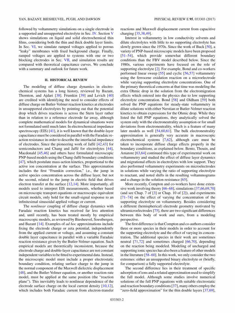
Next, Fig. 4 show a voltammogram for the k = 50 (diffusionlimited) case, with accompanying concentration profiles (c+and c− are identical in the bulk but only c+ is shown).
The parameter δ was chosen to be large for these simulationsso that large diffuse layers do not form, making it easier tosee a correspondence between the slope of the concentrationat the electrode and the resulting current. The current andslope of c+ both reach a maximum when the voltammogrampeaks, followed by a gradual flattening of the concentrationas transport limitation sets in. Furthermore, though we endour simulations in this section after the cation concentrationreaches zero at the electrode, we will see in Sec. V B 3 that thePNP-FBV equations admit solutions past this point with theformation of space charge regions.
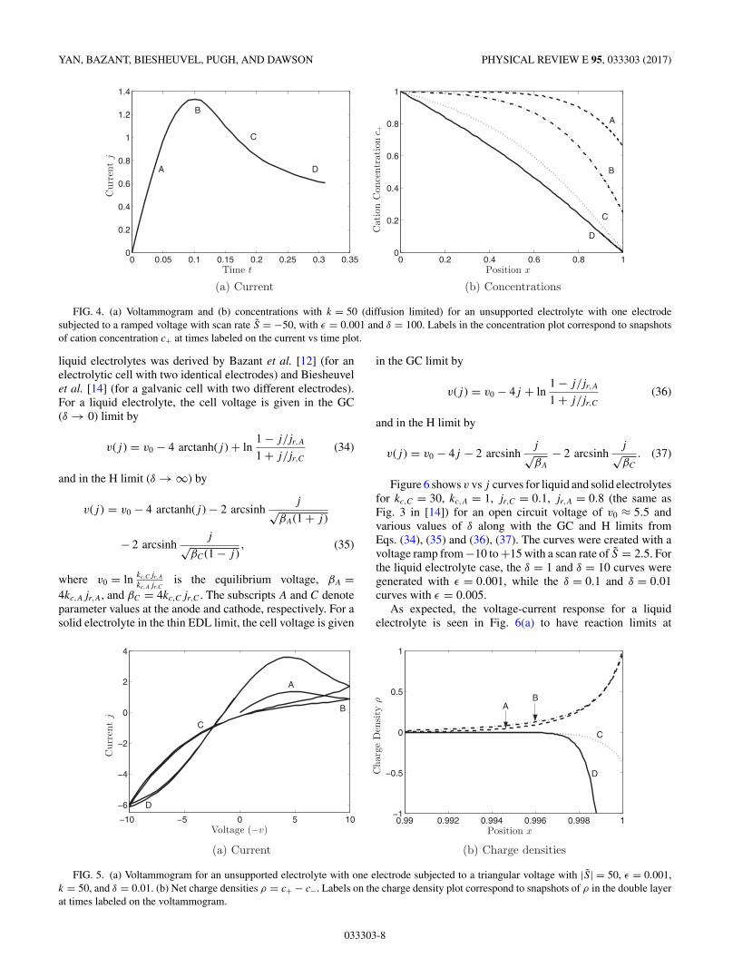
We end this section with Fig. 5, which shows two voltam-metry cycles on a system with ε = 0.001, k = 50, δ = 0.01,and |S| = 50. Due to the fact there is only one electrode andonly one species takes part in the reaction, the voltammogramexhbits diodelike behavior: diffusion limiting in the directionof positive current and exponential growth in the directionof negative current. Also shown are the net charge densities(ρ = c+ − c−) in the diffuse region (x > 0.99) during the firstcycle, which are allowed to form since δ is small, so that thedouble layer is dominated by the diffuse charge region. Theamount of charge separation in the diffuse layer is very largeat large voltages, and highlights the need to use the PNP-FBVequations to capture their dynamics.
Lastly, an interesting observation is that, in Fig. 5, thecurrent peak is much higher in the second (and subsequent)cycle(s) than in the first. We expect that this is due to chargedynamics near the electrode: concentration distributions do notreturn their initial distributions when the polarity of v reverses.Due to the fast scan rate, there is still an excess of positive ionsnear the electrode when the voltage switches polarity at thestart of the second cycle, allowing for a much longer time forthe current to build before transport limitation occurs.
V. LIQUID AND SOLID ELECTROLYTE THIN FILMS
A. Model problem
In this section, we study voltammograms of liquid and solidelectrolyte electrochemical thin films. General steady-statemodels for thin films have been previously presented in[12] and [13] as well as in [14], with a time-dependentmodel considered in [49]. From a modeling perspective,the only difference between the two systems is that thecounterion concentration is constant for solid electrolytes, i.e.,c−(x,t) = 1. Furthermore, for some simulations in this section,we consider voltage ramps on systems with two dissimilarelectrodes, i.e., values of kc and jr such that an equilibriumvoltage develops across the cell.
B. Simulation results
1. Low sweep rates
At low sweep rates, the current-voltage relationship ap-proaches the steady-state response, which for solid and
033303-7
YAN, BAZANT, BIESHEUVEL, PUGH, AND DAWSON PHYSICAL REVIEW E 95, 033303 (2017)
0 0.05 0.1 0.15 0.2 0.25 0.3 0.350
0.2
0.4
0.6
0.8
1
1.2
1.4
Time t
Cur
rent
j
A
B
C
D
(a) Current
0 0.2 0.4 0.6 0.8 10
0.2
0.4
0.6
0.8
1
Position x
Cat
ion
Con
cent
rati
onc +
A
B
C
D
(b) Concentrations
FIG. 4. (a) Voltammogram and (b) concentrations with k = 50 (diffusion limited) for an unsupported electrolyte with one electrodesubjected to a ramped voltage with scan rate S = −50, with ε = 0.001 and δ = 100. Labels in the concentration plot correspond to snapshotsof cation concentration c+ at times labeled on the current vs time plot.
liquid electrolytes was derived by Bazant et al. [12] (for anelectrolytic cell with two identical electrodes) and Biesheuvelet al. [14] (for a galvanic cell with two different electrodes).For a liquid electrolyte, the cell voltage is given in the GC(δ → 0) limit by
v(j ) = v0 − 4 arctanh(j ) + ln1 − j/jr,A
1 + j/jr,C
(34)
and in the H limit (δ → ∞) by
v(j ) = v0 − 4 arctanh(j ) − 2 arcsinhj√
βA(1 + j )
− 2 arcsinhj√
βC(1 − j ), (35)
where v0 = ln kc,Cjr,A
kc,Ajr,Cis the equilibrium voltage, βA =
4kc,Ajr,A, and βC = 4kc,Cjr,C . The subscripts A and C denoteparameter values at the anode and cathode, respectively. For asolid electrolyte in the thin EDL limit, the cell voltage is given
in the GC limit by
v(j ) = v0 − 4j + ln1 − j/jr,A
1 + j/jr,C
(36)
and in the H limit by
v(j ) = v0 − 4j − 2 arcsinhj√βA
− 2 arcsinhj√βC
. (37)
Figure 6 shows v vs j curves for liquid and solid electrolytesfor kc,C = 30, kc,A = 1, jr,C = 0.1, jr,A = 0.8 (the same asFig. 3 in [14]) for an open circuit voltage of v0 ≈ 5.5 andvarious values of δ along with the GC and H limits fromEqs. (34), (35) and (36), (37). The curves were created with avoltage ramp from −10 to +15 with a scan rate of S = 2.5. Forthe liquid electrolyte case, the δ = 1 and δ = 10 curves weregenerated with ε = 0.001, while the δ = 0.1 and δ = 0.01curves with ε = 0.005.
As expected, the voltage-current response for a liquidelectrolyte is seen in Fig. 6(a) to have reaction limits at
−10 −5 0 5 10
−6
−4
−2
0
2
4
Voltage (−v)
Cur
rent
j
A
B
D
C
(a) Current
0.99 0.992 0.994 0.996 0.998 1−1
−0.5
0
0.5
1
Position x
Cha
rge
Den
sity
ρ
C
D
BA
(b) Charge densities
FIG. 5. (a) Voltammogram for an unsupported electrolyte with one electrode subjected to a triangular voltage with |S| = 50, ε = 0.001,k = 50, and δ = 0.01. (b) Net charge densities ρ = c+ − c−. Labels on the charge density plot correspond to snapshots of ρ in the double layerat times labeled on the voltammogram.
033303-8

THEORY OF LINEAR SWEEP VOLTAMMETRY WITH . . . PHYSICAL REVIEW E 95, 033303 (2017)
−1 −0.5 0 0.5 1−10
−5
0
5
10
15
Current j
Vol
tage
v δ = 10
δ = 1
δ = 0.01 δ = 0.1
GC Limit
H Limit
(a) Liquid electrolyte
−1 −0.5 0 0.5 1−10
−5
0
5
10
15
Current j
Vol
tage
v
δ = 3δ = 0.3
δ = 0.1
δ = 1
H Limit
GC Limit
(b) Liquid electrolyte
FIG. 6. v vs j curves for (a) thin EDL liquid electrolyte and (b) thin EDL solid electrolyte with two electrodes and with parametersε = 0.001, kc,C = 30, kc,A = 1, jr,C = 0.1, and jr,A = 0.8 (v0 ≈ 5.5). Also shown are the steady-state curves in the GC and H limits fromEqs. (34), (35) and (36), (37). Simulated curves were created using a voltage scan rate of S = 2.5.
j = −jr,C = −0.1 and j = jr,A = 0.8 in the GC limit, anddiffusion limits at j = ±1 in the H limit. The limiting casesfrom Eqs. (34), (35) also do not strictly bound the simulatedresults in Fig. 6(a) due to the nonmonotonic dependence ofthe cell voltage v on δ [14]. Compared to the liquid electrolytecase, the two limits on δ for fixed countercharge are seenin Fig. 6(b) to have reaction limits at j = −jr,C = −0.2 andj = jr,A = 0.8 in the GC limit, but no diffusion limit in theH limit, which is consistent with the expected behavior for asolid electrolyte.
2. Diffusion and reaction limitating
When sweep rates are fast, current-voltage curves will differfrom the slow sweep results in Sec. V B 1 due to physicallimitation of the speed at which current can be producedat electrodes. This nonlinear interdependence of current andvoltage when current flows into an electrode is describedin electrochemistry by the blanket term polarization, not tobe confused with dielectric polarization. Generally speaking,when current flows across a cell, its cell potential, v, willchange. The difference between the equilibrium value of v
and its value when current is applied is commonly referred toas the overpotential or overvoltage and labeled η.
Very briefly, there are three competing sources of overpo-tential in an electrochemical cell.
(1) Ohmic polarization is caused by the slowness ofelectromigration in the bulk. When a cell behaves primarilyOhmically, it is characterized by a linear j -v curve which canbe written as ηohm = rcellj . When this behavior is modeled bya circuit, it is usually represented as a single resistor betweenthe two electrodes.
(2) Kinetic polarization is due to the slowness of electrodereactions (k small). Using the overpotential version of theButler-Volmer equation as a starting point, and assuming fasttransport of species to and from the electrode (Celectrode =Cbulk), we can invert the equation to find ηkin = arcsinh ( j
j0),
where j0 is the nondimensional exchange current density.
Thus, when kinetic polarization is the primary cause of over-potential, the j -v curve takes on an exponential characteristic.This type of polarization is represented by a charge-transferresistance in circuit models.
(3) Transport, or concentration polarization, is due toslowness in the supply of reactants or removal of productsfrom the electrode, resulting in a depletion of reactantsat the electrode. Concentration polarization is characterizedby a saturation of the current-voltage relationship, and isrepresented by the frequency-dependent Warburg element incircuit models.
In terms of electrode polarization, the key differencebetween liquid and solid electrolytes is that the imposedconstant counterion concentration associated with a solidelectrolyte does not allow diffusion limiting to occur (except,perhaps, with very large forcings), since the reacting speciesis not allowed to be depleted at the electrodes. The trade-off isthat current is only carried by one species in solid electrolytes,increasing the electrolyte resistance.
To illustrate these points, we first show in Fig. 7 Faradaiccurrent vs voltage for liquid and solid electrolyte with twoelectrodes and with parameters ε = 0.05, δ = 1, kc,a = 50,jr,a = 100, kc,c = 0.1, and jr,c = 0.05 (v0 ≈ 1.4). Theseparameters represent a situation with slow reactions at thecathode, and we vary the scan rate S so that reaction limitationwill dominate the current. As S increases, the j -v curves forboth the liquid and solid electrolyte cases are seen to take ona more pronounced exponential character, thus showing theeffect of reaction limitation. When S is small, the Faradaiccurrent in both cases takes a linear or predominantly Ohmiccharacter. Note that for plots where the sweep rate S varies,we only plot the Faradaic part of the current [the second termon the right-hand side of Eq. (19)] since for S � 1 there is asignificant displacement component.
Next, to demonstrate when and how diffusion limitationplays a role, we show in Fig. 8 fast voltage sweeps (S = −100)on both liquid and solid electrolytes with fast reactions (k =50), with accompanying concentration profiles. For liquid
033303-9

YAN, BAZANT, BIESHEUVEL, PUGH, AND DAWSON PHYSICAL REVIEW E 95, 033303 (2017)
0 2 4 6 8 100
0.5
1
1.5
2
Voltage (−v) Voltage (−v)
Far
adai
c C
urre
nt j
f
S = −0.1,−1
S = −10
S = −100
(a) Liquid electrolyte
0 2 4 6 8 100
0.5
1
1.5
2
Far
adai
c C
urre
nt j
f
S = −100
S = −0.1,−1
S = −10
(b) Solid electrolyte
FIG. 7. Faradaic current vs voltage for (a) liquid electrolyte with and (b) solid electrolyte two electrodes and with S varied, with parametersε = 0.05, δ = 1, kc,a = 50, jr,a = 100, kc,c = 0.1, and jr,c = 0.05 (v0 ≈ 1.4). A current response dominated by reaction limitation is seen whenS = −100.
electrolytes [Figs. 8(a) and 8(b)], the current begins to saturateas the cation are depleted at the cathode. Over the same voltagerange, the current in the solid electrolyte [Figs. 8(c) and 8(d)]remains perfectly linear since the fixed negative ions allow formuch less charge separation.
3. Transient space charge
We end our modeling of electrochemical thin films byinvestigating the development of space charge regions (regionsof net charge outside of the double layer where ρ = c+ − c− �=0) at large applied voltages. This is a strongly nonlinear
0 2 4 6 8 100
0.5
1
1.5
2
2.5
Voltage (−v)
Far
adai
c C
urre
nt j
f
B
C
A
D
(a) j vs v, Liquid electrolyte
0 2 4 6 8 100
0.5
1
1.5
2
2.5
Voltage (−v)
Far
adai
c C
urre
nt j
f
A
B
C
D
(b) j vs v, Solid electrolyte
0 0.2 0.4 0.6 0.8 10.2
0.4
0.6
0.8
1
1.2
1.4
1.6
1.8
Position x Position x
Cat
ion
Con
cent
rati
onc +
A
B
C
D
(c) c+, Liquid electrolyte
0 0.2 0.4 0.6 0.8 10.2
0.4
0.6
0.8
1
1.2
1.4
1.6
1.8
Cat
ion
Con
cent
rati
onc +
B
C D
A
(d) c+, Solid electrolyte
FIG. 8. (a), (b) j vs v and (c), (d) cation concentrations c+ at t = 0.025 (dashed line), 0.05 (dash-dotted line), 0.075 (dotted line), and 0.1(solid line) for S = −100 voltage sweeps on both liquid and solid electrolytes with two electrodes. Other parameters are the same as in Fig. 7.
033303-10

THEORY OF LINEAR SWEEP VOLTAMMETRY WITH . . . PHYSICAL REVIEW E 95, 033303 (2017)
−100 −50 0 50 100−3
−2
−1
0
1
2
Voltage (−v)
Cur
rent
j(b) (c)
(d)
(a) Current vs Voltage
0.9 0.92 0.94 0.96 0.98 10
0.05
0.1
0.15
0.2
0.25
0.3
Position x
Con
cent
rati
on c
(b) t=0.1
0.75 0.8 0.85 0.9 0.95 10
0.05
0.1
0.15
0.2
0.25
0.3
Position x
Con
cent
rati
on c
(c) t=0.6
0 0.05 0.1 0.15 0.2 0.250
0.05
0.1
0.15
0.2
0.25
0.3
Position x
Con
cent
rati
on c
(d) t=2.6
FIG. 9. (a) Voltammogram and (b)–(d) resulting cation (solid line) and anion (dashed line) concentrations showing space charge regionsdeveloped at the cathode and anode from a triangular applied voltage in a thin EDL liquid electrolyte with two electrodes. Parameters usedwere ε = 0.001, δ = 0.3, k = 50, and |S| = 100.
effect which occurs in liquid electrolytes as predicted byBazant, Thornton, and Ajdari [38] and solved by Olesen,Bazant, and Bruus using asymptotics and simulations for largesinusoidal voltages [77]. In this section, we extend this work byshowing the formation of space charge regions in the contextof voltammetry by using triangular voltages.
Figure 9(a) shows the voltammogram of a two-electrodeliquid electrolyte system subjected to a triangular voltage withε = 0.001, δ = 0.3, k = 50, and S = 100, and Figs. 9(b)–9(d) show the development of space charge regions. Thecurrent-voltage response during space charge formation is atransient case of a diffusion limited system (S,k � 1) beingdriven above the limiting current [13,24,88] and the subsequentbreakdown of electroneutrality in the bulk. Figure 9 showsthe current peaking as diffusion limiting sets in (t = 0.1) andanion concentration at the cathode reaches zero [Fig. 9(b)].After this time, a space charge region begins to form outsideof the double layer as seen in Fig. 9(c), and the current rampsup slowly until the voltage reverses direction. Since the cellis symmetrical, the same thing occurs at the anode duringthe positive voltage part of the cycle, with current flowingin the other direction [Fig. 9(d)]. The height of the currentpeak and slope of current during space charge development aredependent on the value of S. Also, though the one-dimensional
equations predict it, the formation of large space charge regionsmay not happen in reality due to hydrodynamic instabilitycaused by electrokinetic effects [21,99–102].
VI. LEAKY MEMBRANES
A. Model problem
In this section, we consider the classical description ofmembranes as having constant, uniform background chargedensity ρs , in addition to the mobile ions [103–106]. Inthis section, we focus on the strongly nonlinear regime ofsmall background charge and large currents in a “leakymembrane” [28,107]. This situation can arise as a simpledescription of micro- or nanochannels with charged surfaces,as well as traditional porous media, neglecting electro-osmoticflows. In the case of a microchannel with negative chargeon its sidewalls, surface conduction through the positivelycharged diffuse layers can sustain overlimiting current (fasterthan diffusion) [27] and deionization shock waves [108].This phenomenon has applications to desalination by shockelectrodialysis [29,30], as well as metal growth by shockelectrodeposition [31,32], and the following analysis couldbe used to interpret LSV for such electrochemical systemswith bulk fixed charge.
033303-11

YAN, BAZANT, BIESHEUVEL, PUGH, AND DAWSON PHYSICAL REVIEW E 95, 033303 (2017)
- +
+-
“Leaky” Membrane
-
-- -
-- -
--
-
+
+
+
++
++
++
++
Concentra�on Reservoir
--
--
-
+
++
+
FIG. 10. Sketch of a “leaky” membrane. Left-hand boundary isan ideal reservoir with constant concentration (c+ = c− = 1) andzero potential (φ = 0). Right-hand boundary is an electrode. Mobilecharge is shown with a filled circle; fixed charge (negative in thiscase) is shown without a circle. Also shown are the directions of thevoltage and current density.
Figure 10 shows a sketch of the model problem. A “leaky”membrane with a uniform background charge (negative in thefigure) and with mobile cations and anions lies between anideal reservoir on the left-hand side (c+ = c− = 1, φ = 0) andan electrode on the right. We investigate situations with bothpositive and negative background charge whose concentrationis small compared to that of the mobile ions.
The appropriate modification to the Poisson equation for abackground charge is Eq. (5), which is nondimensionalized to
−2ε2 ∂2φ
∂x2= z+c+ + z−c− + 2ρs , (38)
where ρs = ρs/(2C0F ). Equations (5)–(38) are equivalent tothe “uniform potential model” and “fine capillary model” [109]and have a long history in membrane science [103–105]. Forexample, Tedesco et al. [110] recently used an electroneutralversion of Eq. (38) to model ion exchange membranes forelectrodialysis applications.
The time-independent Nernst-Planck equations can besolved along with Eq. (38) in the limit of thin DL’s to obtainthe steady-state current-voltage relationship [27], which isgiven by
j = 1 − e−|v|/2 − ρs |v|2
, (39)
where the factor of one-half is due to a difference in ourdefinition of the scaling current [in Eq. (19)] from [27].This expression has been successfully fitted to quasisteadycurrent voltage relations in experiments [29,31,32], whichin fact were obtained by LSV at low sweep rates, so it isimportant to understand the effects of finite sweep rates. InSecs. VI B–VI C, we present simulation results for rampedand cyclic voltammetry on systems with background chargeopposite sign (negative background charge) and the same sign(positive background charge) as the reactive ions.
B. Negative background charge
First, we consider the case where the sign of the backgroundcharge is opposite to that of the reactive cations, which avoid
0 2 4 6 8 100
0.1
0.2
0.3
0.4
0.5
0.6
Voltage (−v)
Cur
rent
j
S = −5
Theory
S = −2
S = −3.5
S = −1
FIG. 11. Current in response to a voltage ramp in a liquidelectrolyte with one electrode and constant background charge.Parameters are ε = 0.005, δ = 10, ρs = −0.01, and k = 50. Alsoshown is the steady-state response from Eq. (39).
depletion by screening the fixed background charge. This isthe most interesting case for applications of leaky membranes[29–32], since the system can sustain overlimiting current.Figure 11 shows current in response to voltage ramps withε = 0.005, δ = 10, ρs = −0.01, and k = 50, with variousvalues for S. The limiting behavior for the current for small S
can be predicted by the steady-state response from Eq. (39).As observed in multiple experiments [29,31,32], a bump ofcurrent overshoot occurs prior to steady state for high sweeprates, which we can attribute to diffusion limitation duringtransient concentration polarization in the leaky membrane.Similar bumps have also been predicted by Moya et al. [94] forneutral electrolytes in contact with (nonleaky) ion-exchangemembranes with quasiequilibrium double layers.
Next, Fig. 12 shows a cyclic voltammogram with con-centration profiles for a background charge of ρs = −0.01,with S = 10. Due to the additional background charge, theconcentrations in the bulk are slightly different. For a 1:1electrolyte, this difference is exactly −2ρs , as in Eq. (38). Foran electrolyte that is not 1:1, the difference can be obtainedusing z+c+ + z−c− = −2ρs .
Similar to the cyclic voltammogram in Sec. IV C, thecurrent-voltage relationship in Fig. 12 displays diffusionlimited behavior in the negative voltage sweep direction andpurely exponential growth (reaction limiting behavior) in theother. This is because there is only one electrode in thesesimulations with only one of the two species taking part in thereaction.
C. Positive background charge
For positive ρs , Eq. (39) predicts a decreasing current(or negative steady-state differential resistance) after theexponential portion, a behavior which has been observed insome experiments [31,32] and not others [29]. Interestingly,when double-layer effects and electrode reaction kinetics areconsidered in the model simulations, the region of negativeresistance is also not observed, as shown in Fig. 13 for
033303-12

THEORY OF LINEAR SWEEP VOLTAMMETRY WITH . . . PHYSICAL REVIEW E 95, 033303 (2017)
−10 −5 0 5 10−20
−15
−10
−5
0
5
Voltage (−v)
Cur
rent
j
(c)
(d) (b)
(a) Voltammogram
0 0.2 0.4 0.6 0.8 10
0.2
0.4
0.6
0.8
1
Position x
Position xPosition x
Con
cent
rati
on c
Con
cent
rati
on c
Con
cent
rati
on c
(b) v=-3.3, t=0.33
0 0.2 0.4 0.6 0.8 11
2
3
4
5
6
(c) v=5, t=2.5
0 0.2 0.4 0.6 0.8 11
2
3
4
5
6
7
8
(d) v=0, t=4, second cycle
FIG. 12. (a) Voltammogram and (b)–(d) resulting cation (solid line) and anion (dashed line) concentrations for a thin EDL liquid electrolytewith two electrodes and constant negative background charge. Parameters used were ε = 0.005, δ = 1, k = 50, ρs = −0.01, and |S| = 10.Two cycles are shown in (a).
ρs = 0.01. Physically, the interfaces provide overall positivedifferential resistance, even as the bulk charged electrolyte
0 2 4 6 8 100
0.1
0.2
0.3
0.4
0.5
0.6
Voltage (−v)
Cur
rent
j
Theory
S = −5S = −3.5
S = −1
S = −2
FIG. 13. Current from a voltage ramp applied to a liquidelectrolyte with a single electrode and constant, small, positivebackground charge. Parameters are ε = 0.005, δ = 10, ρs = 0.01,and k = 50. Also shown is the steady-state response from Eq. (39),which is shown not to match the simulations.
enters the overlimiting regime with negative local steady-statedifferential resistance.
Lastly, we omit the plot of the two-cycle voltammogramfor positive background charge, and just remark that theyshow results which are very similar to the voltammogram inFig. 12(a).
VII. BLOCKING ELECTRODES
A. Model problem
A blocking, or ideally polarizable, electrode is one whereno Faradaic reactions take place. From a modeling perspective,this means setting kc and jr in the Butler-Volmer equation tozero, so that current is entirely due to the displacement currentterm in Eq. (19).
Voltammetry experiments are most often used to probeFaradaic reactions at test electrodes; in this application, non-Faradaic or charging current is undesirable. With that beingsaid, however, linear sweep voltammetry is also a standardapproach to measuring differential capacitance. Much of theearly work in electrochemistry was centered around matchingexperimental differential capacitance curves with theory. Gouy[111] and Chapman [112] independently solved the Poisson-Boltzmann equation to obtain the differential capacitance per
033303-13

YAN, BAZANT, BIESHEUVEL, PUGH, AND DAWSON PHYSICAL REVIEW E 95, 033303 (2017)
unit area for an electrode in a 1:1 liquid electrolyte, which inthe present notation can be written as
Cliquid(�φ) = 1
εcosh
�φ
2, (40)
where �φ is the diffuse layer. Later, Kornyshev and Vorotynt-sev [34] performed a similar calculation for a solid electrolyte(an electrolyte where one ion is fixed in position with ahomogeneous distribution) to obtain
Csolid(�φ) = 1
ε
1 − e−�φ√e−�φ + �φ − 1
sgn(�φ). (41)
Note that the capacitance for the liquid electrolyte is symmet-rical about zero, but the capacitance for the solid electrolyte isnot symmetrical due to the fixed charge breaking the symmetry.
In this section, we use ramped voltages to investigate thebehavior of blocking electrodes for liquid and solid electrolyteswith thin and thick double layers. Similar work has been doneby Bazant et al. [38], who used asymptotics to study diffusecharge effects in a system with blocking electrodes subjected toa step voltage, Olesen et al. [77], who used both asymptoticsand simulations to do the same for sinusoidal voltages, andrecently by Feicht et al. [113], who studied dynamics for high-to-low voltage steps. In this section, we present simulations forramped voltage boundary conditions. The results of this sectionhave applications to EDL supercapacitors [114], capacitivedeionization [115,116], and induced charge electro-osmotic(ICEO) flows [81,101]. In the simulations in this section, δ isset to 0.01 so that the capacitance is dominated by the diffusepart of the double layer.
The displacement current in Eq. (19) is related to thenondimensionalized capacitance through
j = −ε2
2
dφx
dt= ε2
2
dq
dt= ε2
2
dq
dv
dv
dt, (42)
where q = − dφ
dxis the surface charge density and dv
dt= S.
Since C = dq
dv, we have that
j
S= ε2
2C ∼ ε
2(43)
and therefore ε is the natural scale for capacitance whenrelating to the displacement current. We refer to this as our“rescaled” capacitance, which we denote using the symbol C.
Both solid and liquid electrolyte systems with two blockingelectrodes behave like the circuit shown in Fig. 14. For liquid
+−
v(t)
j
C
+−Δφ
R
+−
C
−+Δφ
FIG. 14. Equivalent circuit diagram for system with two blockingelectrodes, showing the defined direction of current and polarities ofthe double layer capacitors. Note that C is a function of �φ.
electrolytes, R ∼ 2 and C(0) = ε/2. For solid electrolytes,R ∼ 4 [12,14] and C(0) = ε2
2 lim�φ→0 Csolid(�φ) =√
2ε2 .
There are two regimes of operation when a ramped voltageis applied to a capacitive system. The first is the small time(t � ε) behavior, when the double layers are charged withtime constant τRC = RC/2, where the factor of 1/2 accountsfor the fact that there are two capacitors in series. To predict thebehavior during this time, we turn to the ordinary differentialequation describing the circuit in Fig. 14, which is
v(t) − 2�φ = RC(0)d�φ
dt, (44)
where v(t) = St . From Eq. (44), the current can be solved inthe case of a two-electrode liquid electrolyte to be
2jinner(t)
S= C(0)
(1 − e
− v
SC(0)), (45)
where we have used R = 2 for a liquid electrolyte. Theequivalent expression for solid electrolytes with single anddouble electrodes will be discussed in Sec. VII B. The secondregime of operation is the large time (t � ε) behavior. Afterthe RC charging time, the current tracks the capacitance basedon Eq. (43). The relevant equation is
j = ε2
2
dq
dt= C(�φ)
d�φ
dt. (46)
Since we are only able to control the potential drop acrossthe cell [v(t)] and not the potential drop across the doublelayer (�φ), we must estimate the value of �φ by accountingfor the potential drop across the bulk. To do this, we can usethe equation v(t) = 2�φ + Rj . In practice, however, j � 1for blocking electrodes and so we can instead just use �φ ≈v(t)/2 = St/2. Equation (46) can then be rewritten as
2jouter
S= C(v/2). (47)
From Eq. (45) we have a solution for small times (the innersolution), and from Eq. (47) we have a solution for large times(the outer solution). The long time limit for the inner solutionmust be equal to the small time limit for the outer solution,and so the two solutions can be combined by adding them andsubtracting the overlap,
j = jinner + jouter − joverlap, (48)
where 2joverlap/S = C(0), thereby creating a uniformly validapproximation of the capacitance for all values of v(t).
B. Simulation results
We begin by presenting the uniformly valid approximations[Eq. (48)] for liquid and solid electrolytes. For a liquidelectrolyte with two electrodes, the current takes the form
2j
S= C
(1 − e
v
SC
) + ε
2cosh
v
4− C, (49)
where C = ε/2. The situation for solid electrolytes ismore complicated: since the capacitance [Eq. (41)] is not
033303-14

THEORY OF LINEAR SWEEP VOLTAMMETRY WITH . . . PHYSICAL REVIEW E 95, 033303 (2017)
0 1 2 3 4 5 6 70
0.5
1
1.5x 10
−3
−v
2j/S
(a) Liquid, Thin EDL
0 2 4 6 8 100
0.02
0.04
0.06
0.08
0.1
−v
2 j/S
(b) Liquid, Thick EDL
0 2 4 6 8 100
1
2
3
4x 10
−4
−v
2j/S
(c) Solid, Thin EDL
0 2 4 6 8 100
0.005
0.01
0.015
0.02
0.025
0.03
0.035
−v
2j/S
(d) Solid, Thick EDL
FIG. 15. Simulated (solid lines) and uniformly valid approximation (dashed lines) j vs v curves for two-electrode liquid electrolyte with(a) thin and (b) thick double layers, as well as two-electrode solid electrolyte with (c) thin and (d) thick double layers. Plots with δ = 0.01 andS = −10 are shown. Dashed lines are plotted from Eqs. (49) and (52).
symmetrical about �φ = 0, the capacitance for a solid elec-trolyte system with two blocking electrodes can be representedusing two capacitors in series,
1
Csolid(�φ)= 1
Csolid(�φ)+ 1
Csolid(−�φ). (50)
The uniformly valid approximation for a solid electrolyte withone electrode is
j
S= C
(1 − e
v
SC
) + ε1 − e−v
√e−v + v − 1
sgn (v) − C, (51)
where C = √2ε. Using Eq. (50), the approximation for two
electrodes is
2j
S= C
(1 − e
v
2SC
) + ε
2
⎛⎝ 1 − e− v
2√e− v
2 + v2 − 1
sgn (v)
∣∣∣∣∣∣∣∣∣∣∣∣
1 − ev2√
ev2 − v
2 − 1sgn (−v)
⎞⎠ − C, (52)
where C = ε
2√
2and || indicates the reciprocal of the sum of
the reciprocals, i.e., A||B = 1/(1/A + 1/B). The additionalfactor of 1/2 in the exponent in the inner part of Eq. (52) is dueto the fact that the electrolyte resistance for solid electrolytesis 4 rather than 2.
Figure 15 shows j -v curves for thin EDL (ε = 0.001) andthick EDL (ε = 0.1) liquid and solid electrolyte systems withtwo electrodes. The plots are compared to the approximations
from Eqs. (49) and (52), and show generally good agreement,except for Fig. 15(b), the liquid, thick EDL case.
The reason for this is that the approximation in Eq. (49)is based on an equilibrium (Gouy-Chapman) picture of theEDL. With thick EDL liquid electrolytes under large voltageforcings, so much charge separation occurs that the systemis too far from equilibrium for the Gouy-Chapman modelto be valid. To investigate further, we plot in Fig. 16 the
033303-15

YAN, BAZANT, BIESHEUVEL, PUGH, AND DAWSON PHYSICAL REVIEW E 95, 033303 (2017)
0 2 4 6 8 100
0.005
0.01
0.015
0.02
0.025
0.03
0.035
0.04
−v
2j/S
A
D
B
C
(a) Current vs voltage, S = −0.1
0 0.2 0.4 0.6 0.8 10
0.5
1
1.5
2
Position x
Cat
ion
Con
cent
rati
onc +
A
C
B
D
(b) Cation concentrations
FIG. 16. (a) j vs v and (b) cation concentrations for a thick EDL liquid electrolyte with two blocking electrodes and parameters ε = 0.1,δ = 0.01 and scan rate S = −0.1. Labels in (a) correspond to cation concentrations in (b) at various times.
current resulting from a voltage sweep of S = −0.1 on aliquid electrolyte system with ε = 0.1 along with cationconcentrations at various points during the sweep. We canseparate the behavior in Fig. 16 into three regimes. For
small voltages (A), the concentrations show near-equilibriumbehavior. As the voltage increases (B), (C), the diffuse regionsbecome large and the bulk concentration begins to be depleted,and the two double layers begin to overlap—it may be possible
0 1 2 3 40
1
2
3
4
5
6
7
8x 10
−3
−v
j/S
(a) Negative voltage sweep
0 2 4 6 8 100
0.5
1
1.5x 10
−3
v
j/S
(b) Positive voltage sweep
0 2 4 6 8 100
0.5
1
1.5
2
−v
j/S
(c) Negative voltage sweep
0 2 4 6 8 100
0.02
0.04
0.06
0.08
0.1
0.12
0.14
v
j/S
(d) Positive voltage sweep
FIG. 17. Simulated (solid lines) vs uniformly valid approximation (dashed lines) j vs v curves for (a), (b) thin EDL solid electrolyte and(c), (d) thick EDL solid electrolyte with a single blocking electrode. δ = 0.01 and S = ±1. Figures (a) and (c) show the negative part of thesweep and (b) and (d) show the positive part. Dashed lines are plotted from Eq. (51).
033303-16

THEORY OF LINEAR SWEEP VOLTAMMETRY WITH . . . PHYSICAL REVIEW E 95, 033303 (2017)
to model behavior at this stage by accounting for the depletionof bulk concentration as in [38]. Finally, at large voltages(D), we see complete charge separation, with nearly all ofthe positive charge located at the cathode (and, similarly,with nearly all of the negative charge at the anode). Thisis the result which highlights the need to model diffusecharge dynamics using the PNP-FBV equations; such a highlynonlinear separation of charge would not be predicted bymodels which assume electroneutrality or neglect the couplingbetween diffuse charge dynamics and electrode currents.
It is interesting to note that such a departure from equi-librium behavior is not apparent for the thick EDL solidelectrolyte shown in Fig. 15(d). However, if we plot thesingle electrode, thick EDL curves [shown in Fig. 17(c) forthe negative sweep and Fig. 17(d) for the positive sweep],we see that there is indeed a departure from the equilibriumcapacitance curve for the positive voltage (S = 1) sweep, withthe simulated capacitance having nonmonotonic dependenceon voltage. This disagreement is masked by the fact that, fortwo electrodes [which can be thought of as two capacitorsin series, as in Eq. (52)], the smaller, positive voltage sweepcapacitance, which agrees with the equilibrium approximation,dominates. Figure 17 also shows the single-electrode resultsfor a thin EDL solid electrolyte, which agree with theequilibrium approximation.
We end by remarking that, despite some disagreementsin the thick EDL cases, every simulation showed very goodagreement with the approximations we used during the RCcharging portion of the curve, i.e., the inner solution in Eq. (48).
VIII. CONCLUSIONS AND FUTURE WORK
This paper provides a general theory to enable the useof LSV or CV to characterize electrochemical systems withdiffuse charge. Our paper presents and extends theory andsimulations in a variety of situations which extend classicalinterpretations (unsupported liquid electrolytes and systemswith blocking electrodes) and develop an understanding formore complicated situations (thin films, systems where bulkelectroneutrality breaks down with space charge formation,and leaky membranes). Following a thorough historical review,we began with single-electrode voltammograms for supportedelectrolytes, with an analytical expression in the limit of fastreactions, as well as for unsupported electrolytes in the limitof small ε. We showed for these systems where inclusion ofdiffuse charge dynamics plays a larger role, namely when asystem with small δ has a large voltage applied.
Next, we applied ramped voltages to solid and liquid thinfilms to obtain current-voltage relationships and discussed theeffect of various types of polarization, and how their effect onthe current differed between liquid and solid electrolytes. Forliquid electrolytes, we also observed the formation of spacecharge regions at large voltages, another prediction whichis made possible by using the PNP-FBV equations. For ourleaky membrane model simulations, we found that simulationsmatched a steady-state analytical expression reasonably wellwhen the background charge was opposite in polarity tothe reactive ion (negative background charge) but did notmatch theory with positive background charge. We ended bypresenting analytical expressions for the capacitance of liquid
and solid electrolyte systems with blocking electrodes, andcompared them to simulations with both thin and thick doublelayers. We found that our analytical approximations workedwell for thin double layers, but in some cases disagreed whendouble layers were thick. In general, we conclude that diffusecharge dynamics becomes important in voltammetry at largeapplied voltages and/or with thick double layers.
For each type of system we considered, the simulationresults we obtained were compared to limiting cases andwe showed where simple analytical expressions can beused to predict behavior (such as approximating capacitancecurves), and which regimes require more careful analysis andsimulation. This is of practical interest for electrochemists andengineers, for whom it can assist in guiding the design of newdevices and experiments.
For future work, there are many ways to extend the modelfor additional physics. For example, specific adoption of ionscould be added to the boundary conditions, providing anadditional mechanism for charge regulation of the surface[29,117,118], in addition to Faradaic polarization, coupledthrough the FBV equations. The PNP ion transport equationscould be extended to include recombination bulk reactions(ion-ion, ion-defect, etc.) [16] or various models of ion crowd-ing effects [81,119–121] or other nonidealities in concentratedsolutions. There is also the possibility of coupled masstransport fluxes (Maxwell Stefan, dusty gas, etc.) [122], whichbecome important in concentrated electrolytes [7], as well asfor unequal diffusion coefficients. Poisson’s equation couldalso be modified to account for electrostatic correlations [123]or dielectric polarization effects [124]. Furthermore, while weused generalized BV kinetics [96] in this work, Marcus kinetics[1,125] may provide a more accurate model of charge transferreactions. Even keeping the same PNP-FBV framework, itwould be interesting to extend the model for 2D or 3D geome-tries, convection, and moving boundaries, in order to describeconversion batteries, electrodeposition, and corrosion.
APPENDIX: DERIVATION OF MODIFIEDRANDLES-SEVCIK EQUATION
In this Appendix, we solve the semi-infinite diffusion equa-tion with a nonhomogeneous boundary condition. The resultwe obtain is referenced in Sec. IV B as an analog to the originalRandles-Sevcik function for a single ion electrodepositionreaction. The method used here is taken from Chap. 5.5 ofO’Neil [126]. The equation and boundary conditions are
ut = uxx, (A1)
u(x,0) = A for x > 0, (A2)
u(0,t) = f (t) [where f (0) = A]. (A3)
We begin by considering the same problem with a jump at theboundary at time t = t0:
ut = uxx, (A4)
u(x,0) = A for x > 0, (A5)
u(0,t) ={A 0 < t < t0,
B t > t0,(A6)
033303-17
YAN, BAZANT, BIESHEUVEL, PUGH, AND DAWSON PHYSICAL REVIEW E 95, 033303 (2017)
where A, B are positive constants. u(0,t) can be written withthe Heaviside step function H (t) as
u(0,t) = A(1 − H (t − t0)) + BH (t − t0). (A7)
The PDE (A4)–(A6) can be solved via Laplace transform.The Laplace transform of Eq. (A4) is
sU (x,s) − A = ∂xxU (x,s), (A8)
where U (x,s) = L u(x,t). The general solution of Eq. (A8),a constant-coefficient second order ODE for U , is
U (x,s) = a(s)e√
sx + b(s)e−√sx + A
s. (A9)
We impose the condition a(s) = 0 because we would like thesolution to be bounded as x → ∞. This leaves us to solve forb(s) using the boundary condition [Eq. (A7)]. The Laplacetransform of Eq. (A7) is
L u(0,t) = A
s− A
se−t0s + B
se−t0s . (A10)
Using Eq. (A10), b(s) can be solved to be
b(s) = B − A
se−t0s , (A11)
giving us
U (x,s) = B − A
se−t0se−√
sx + A
s. (A12)
We can now take the inverse Laplace transform of Eq. (A12)to obtain
u(x,t) = A + (B − A) erfc
(x
2√
t − t0
), (A13)
where erfc(z) = 1 − erf(z) = 2√π
∫ ∞z
exp (x2) dx is thecomplementary error function. In other words, the solution to
the semi-infinite diffusion problem with a jump of �u(0,t0)relative to A at x = 0 and time t = t0 is
u(x,t) = A + �u(0,t0) erfc
(x
2√
t − t0
). (A14)
Now, using Duhamel’s principle, we have for an arbitraryseries of steps at t = ti given by �u(0,ti) = f (ti),
u(x,t) = A +∑
i
�f (ti) erfc
(x
2√
t − ti
), (A15)
where �f (ti) = f (ti+1) − f (ti). We can take the continuumlimit with �f (ti) = df
dt(ti)�ti , where ti < ti < ti+1, to obtain
u(x,t) = A +∫ t
0
df
dt(t ′) erfc
(x
2√
t − t ′
)dt ′ (A16)
and finally we can make the substitution τ = t − t ′ to write
u(x,t) = A −∫ 0
t
df
dt(t − τ ) erfc
(x
2√
τ
)dτ
= A +∫ t
0
df
dt(t − τ ) erfc
(x
2√
τ
)dτ. (A17)
Equation (A17) may be numerically integrated. Alternatively,if we are interested in the Nernstian function, f (t) = e−St
[for quasiequilibrium fast reactions, as in Eq. (28)] and wishto compute the resulting current j = ux(0,t), we can arrive atan analytical expression for ux(0,t),
ux(x,t) = S e−St
∫ t
0
eSτ e− x2
4τ√πτ
dτ, (A18)
ux(0,t) =√
Se−St erfi(√
St), (A19)
where erfi(z) = 2√π
∫ z
0 exp (x2) dx is the imaginary errorfunction.
[1] A. J. Bard and L. R. Faulkner, Electrochemical Methods:Fundamentals and Applications (John Wiley & Sons, NewYork, 2001).
[2] R. G. Compton and C. E. Banks, Understanding Voltammetry(Imperial College Press, London, 2011).
[3] R. G. Compton, E. Laborda, and K. R. Ward, UnderstandingVoltammetry: Simulation of Electrode Processes (ImperialCollege Press, London, 2014).
[4] J. E. B. Randles, Discuss. Faraday Soc. 1, 11 (1947).[5] J. E. B. Randles, Trans. Faraday Soc. 44, 327 (1948).[6] A. Sevcik, Collect. Czech. Chem. Commun. 13, 349
(1948).[7] J. Newman and K. E. Thomas-Alyea, Electrochemical Systems
(John Wiley & Sons, Hoboken, NJ, 2012).[8] P. Simon and Y. Gogotsi, Nat. Mater. 7, 845 (2008).[9] P. M. Biesheuvel and M. Z. Bazant, Phys. Rev. E 81, 031502
(2010).[10] P. M. Biesheuvel, Y. Fu, and M. Z. Bazant, Phys. Rev. E 83,
061507 (2011).[11] P. M. Biesheuvel, Y. Fu, and M. Z. Bazant, Russian J.
Electrochem. 48, 580 (2012).
[12] M. Z. Bazant, K. T. Chu, and B. J. Bayly, SIAM J. Appl. Math.65, 1463 (2005).
[13] K. T. Chu and M. Z. Bazant, SIAM J. Appl. Math. 65, 1485(2005).
[14] P. M. Biesheuvel, M. van Soestbergen, and M. Z. Bazant,Electrochem. Acta 54, 4857 (2009).
[15] M. van Soestbergen, Russian J. Electrochem. 48, 570 (2012).[16] A. C. Luntz, J. Voss, and K. Reuter, J. Phys. Chem. Lett. 6,
4599 (2015).[17] J.-M. Tarascon and M. Armand, Nature (London) 414, 359
(2001).[18] R. Muralidhar, T. Shaw, F. Chen, P. Oldiges, D. Edelstein, S.
Cohen, R. Achanta, G. Bonilla, and M. Bazant, in 2014 IEEEInternational Reliability Physics Symposium (IEEE, New York,2014).
[19] P. M. Biesheuvel, A. A. Franco, and M. Z. Bazant, J.Electrochem. Soc. 156, B225 (2009).
[20] A. A. Franco, P. Schott, C. Jallut, and B. Maschke, Fuel Cells7, 99 (2007).
[21] M. Z. Bazant and T. M. Squires, Phys. Rev. Lett. 92, 066101(2004).
033303-18

THEORY OF LINEAR SWEEP VOLTAMMETRY WITH . . . PHYSICAL REVIEW E 95, 033303 (2017)
[22] T. M. Squires and S. R. Quake, Rev. Mod. Phys. 77, 977 (2005).[23] R. B. Schoch, J. Han, and P. Renaud, Rev. Mod. Phys. 80, 839
(2008).[24] I. Rubinstein and L. Shtilman, J. Chem. Soc., Faraday Trans. 2
75, 231 (1979).[25] I. Rubinstein, E. Staude, and O. Kedem, Desalination 69, 101
(1988).[26] V. V. Nikonenko, N. D. Pismenskaya, E. I. Belova, P. Sistat, P.
Huguet, G. Pourcelly, and C. Larchet, Adv. Colloid InterfaceSci. 160, 101 (2010).
[27] E. V. Dydek, B. Zaltzman, I. Rubinstein, D. S. Deng, A. Mani,and M. Z. Bazant, Phys. Rev. Lett. 107, 118301 (2011).
[28] E. V. Dydek and M. Z. Bazant, AlChE J. 59, 3539 (2013).[29] D. Deng, E. V. Dydek, J.-H. Han, S. Schlumpberger, A. Mani,
B. Zaltzman, and M. Z. Bazant, Langmuir 29, 16167 (2013).[30] S. Schlumpberger, N. B. Lu, M. E. Suss, and M. Z. Bazant,
Environ. Sci. Technol. Lett. 2, 367 (2015).[31] J.-H. Han, E. Khoo, P. Bai, and M. Z. Bazant, Sci. Rep. 4, 7056
(2014).[32] J. H. Han, M. Wang, P. Bai, F. R. Brushett, and M. Z. Bazant,
Sci. Rep. 6, 28054 (2016).[33] E. Itskovich, A. A. Kornyshev, and M. A. Vorotyntsev, Phys.
Status Solidi A 39, 229 (1977).[34] A. A. Kornyshev and M. A. Vorotyntsev, Electrochim. Acta
26, 303 (1981).[35] A. Bonnefont, F. Argoul, and M. Z. Bazant, J. Electroanal.
Chem. 500, 52 (2001).[36] R. He, S. Chen, F. Yang, and B. Wu, J. Phys. Chem. B 110,
3262 (2006).[37] I. Streeter and R. G. Compton, J. Phys. Chem. C 112, 13716
(2008).[38] M. Z. Bazant, K. Thornton, and A. Ajdari, Phys. Rev. E 70,
021506 (2004).[39] A. Frumkin, Z. Phys. Chem. 164A, 121 (1933).[40] V. G. Levich, Dokl. Akad. Nauk SSSR 67, 309 (1949).[41] E. Barsoukov and J. R. Macdonald, Impedance Spectroscopy:
Theory, Experiment, and Applications (Wiley, Hoboken, 2005).[42] G. Jaffe, Ann. Phys. (NY) 408, 249 (1933).[43] G. Jaffe, Phys. Rev. 85, 354 (1952).[44] H.-C. Chang and G. Jaffe, J. Chem. Phys. 20, 1071 (1952).[45] J. R. Macdonald, J. Chem. Phys. 58, 4982 (1973).[46] J. R. Macdonald and D. R. Franceschetti, J. Chem. Phys. 68,
1614 (1978).[47] J. R. Macdonald, J. Phys. Chem. A 115, 13370 (2011).[48] J. D. Jackson, Classical Electrodynamics (Wiley, New York,
1962).[49] M. van Soestbergen, P. M. Biesheuvel, and M. Z. Bazant, Phys.
Rev. E 81, 021503 (2010).[50] R. P. Buck, J. Electroanal. Chem. Interfacial Electrochem. 46,
1 (1973).[51] J. D. Norton, H. S. White, and S. W. Feldberg, J. Phys. Chem.
94, 6772 (1990).[52] W. D. Murphy, J. A. Manzanares, S. Mafe, and H. Reiss, J.
Phys. Chem. 96, 9983 (1992).[53] C. P. Smith and H. S. White, Anal. Chem. 65, 3343 (1993).[54] K. B. Oldham and A. M. Bond, J. Electroanal. Chem. 508, 28
(2001).[55] A. M. Bond, M. Fleischmann, and J. Robinson, J. Electroanal.
Chem. 168, 299 (1984).
[56] A. M. Bond and P. A. Lay, J. Electroanal. Chem. 199, 285(1985).
[57] A. M. Bond, D. C. Coomber, S. W. Feldberg, K. B. Oldham,and T. Vu, Anal. Chem. 73, 352 (1984).
[58] A. M. Bond, M. Fleischmann, and J. Robinson, J. Electroanal.Chem. 172, 11 (1984).
[59] K. B. Oldham, J. Electroanal. Chem. 250, 1 (1998).[60] J. C. Myland and K. B. Oldham, Electrochem. Comm. 1, 467
(1999).[61] K. B. Oldham and S. W. Feldberg, J. Phys. Chem. B 103, 1699
(1999).[62] K. B. Oldham, F. Marken, and J. C. Myland, J. Solid State
Electrochem. 20, 3083 (2016).[63] M. F. Bento, L. Thouin, C. Amatore, and M. I. Montenegro, J.
Electroanal. Chem. 443, 137 (1998).[64] C. Amatore, L. Thouin, and M. F. Bento, J. Electroanal. Chem.
463, 45 (1999).[65] M. F. Bento, L. Thouin, and C. Amatore, J. Electroanal. Chem.
446, 91 (1998).[66] E. J. F. Dickinson and R. G. Compton, J. Electroanal. Chem.
661, 198 (2011).[67] E. J. F. Dickinson, J. G. Limon-Petersen, and R. G. Compton,
J. Solid State Electrochem. 15, 1335 (2011).[68] C. Batchelor-McAuley, E. Katelhon, E. O. Barnes, R. G.
Compton, E. Laborda, and A. Molina, ChemistryOpen 4, 224(2015).
[69] E. J. F. Dickinson and R. G. Compton, Chem. Phys. Lett. 497,178 (2010).
[70] S. R. Belding and R. G. Compton, J. Electroanal. Chem. 683,1 (2012).
[71] J. G. Limon-Petersen, I. Streeter, N. V. Rees, and R. G.Compton, J. Phys. Chem. C 112, 17175 (2008).
[72] J. G. Limon-Petersen, I. Streeter, N. V. Rees, and R. G.Compton, J. Phys. Chem. C 113, 333 (2009).
[73] S. R. Belding, J. G. Limon-Petersen, E. J. F. Dickinson, andR. G. Compton, Angew. Chem., Int. Ed. 49, 9242 (2010).
[74] E. J. F. Dickinson, J. G. Limon-Petersen, N. V. Rees, and R. G.Compton, J. Phys. Chem. C 113, 11157 (2009).
[75] K. Aoki, Electroanalysis 5, 627 (1993).[76] O. Stern, Z. Electrochem. 30, 508 (1924).[77] L. H. Olesen, M. Z. Bazant, and H. Bruus, Phys. Rev. E 82,
011501 (2010).[78] M. van Soestbergen, Electrochem. Comm. 20, 105 (2012).[79] M. A. G. Zevenbergen, B. L. Wolfrum, E. D. Goluch, P. S.
Singh, and S. G. Lemay, J. Am. Chem. Soc. 131, 11471(2009).
[80] M. A. G. Zevenbergen, P. S. Singh, E. D. Goluch, B.L. Wolfrum, and S. G. Lemay, Anal. Chem. 81, 8203(2009).
[81] M. Z. Bazant, M. S. Kilic, B. D. Storey, and A. Ajdari, Adv.Colloid Interfac. Sci. 152, 48 (2009).
[82] L. H. Olesen, H. Bruus, and A. Ajdari, Phys. Rev. E 73, 056313(2006).
[83] L. H. Olesen, Ph.D. thesis, Danish Technical University, 2006.[84] J. L. Moran and J. D. Posner, J. Fluid Mech. 680, 31 (2011).[85] J. L. Moran, P. M. Wheat, and J. D. Posner, Phys. Rev. E 81,
065302 (2010).[86] B. M. Grafov and A. A. Chernenko, Dokl. Akad. Nauk. SSSR
146, 135 (1962) [English translation, pp. 629–632].
033303-19

YAN, BAZANT, BIESHEUVEL, PUGH, AND DAWSON PHYSICAL REVIEW E 95, 033303 (2017)
[87] J. Newman and W. H. Smyrl, Trans. Faraday Soc. 61, 2229(1965).
[88] W. H. Smyrl and J. Newman, Trans. Faraday Soc. 63, 207(1966).
[89] A. D. MacGillivray, J. Chem. Phys. 48, 2903 (1968).[90] I. Rubinstein and B. Zaltzman, Math. Modell. Meth. Appl. Sci.
11, 263 (2001).[91] B. Zaltzman and I. Rubinstein, J. Fluid Mech. 579, 173
(2007).[92] D. R. Baker and M. W. Verbrugge, Proc. R. Soc. London A
454, 1805 (1997).[93] G. Richardson and J. R. King, J. Eng. Math. 59, 239 (2007).[94] A. A. Moya, E. Belashova, and P. Sistat, J. Membrane Sci. 474,
215 (2015).[95] T. B. Grimley and N. F. Mott, Discuss. Faraday Soc. 1, 3 (1947).[96] M. Z. Bazant, Acc. Chem. Res. 46, 1144 (2013).[97] J. J. Bikerman, Philos. Mag. 33, 384 (1942).[98] N. F. Carnahan and K. E. Starling, J. Chem. Phys. 51, 635
(1969).[99] D. Wang and S. J. Ruuth, J. Comput. Math. 26, 838 (2008).
[100] U. M. Ascher, S. J. Ruuth, and B. T. R. Wetton, SIAM J. Numer.Anal. 32, 797 (1995).
[101] M. Z. Bazant and T. M. Squires, Curr. Opin. Colloid InterfaceSci. 15, 203 (2010).
[102] J. A. Levitan, S. Devasenathipathy, V. Studere, Y. Ben, T.Thorsen, T. M. Squires, and M. Z. Bazant, Colloids Surf. A267, 122 (2005).
[103] T. Teorell, Exp. Biol. Med. 33, 282 (1935).[104] K. H. Meyer and J. F. Sievers, Helv. Chem. Acta 19, 649 (1936).[105] K. S. Spiegler, Desalination 9, 367 (1971).[106] R. Abu-Rjal, V. Chinaryan, M. Z. Bazant, I. Rubinstein, and B.
Zaltzman, Phys. Rev. E 89, 012302 (2014).[107] A. Yaroshchuk, Adv. Colloid Interface Sci. 183–184, 68
(2012).
[108] A. Mani and M. Z. Bazant, Phys. Rev. E 84, 061504 (2011).[109] P. B. Peters, R. van Roij, M. Z. Bazant, and P. M. Biesheuvel,
Phys. Rev. E 93, 053108 (2016).[110] M. Tedesco, H. M. V. Hamelers, and P. M. Biesheuvel, J.
Membr. Sci. 510, 370 (2016).[111] M. Gouy, J. Phys. Theor. Appl. 9, 457 (1910).[112] D. L. Chapman, Philos. Mag. 25, 475 (1913).[113] S. E. Feicht, A. E. Frankel, and A. S. Khair, Phys. Rev. E 94,
012601 (2016).[114] A. A. Lee, S. Kondrat, G. Oshanin, and A. A. Kornyshev,
Nanotechnology 25, 315401 (2014).[115] S. Porada, R. Zhao, A. van der Wal, V. Presser, and P. M.
Biesheuvel, Prog. Mater. Sci. 58, 1388 (2013).[116] R. Zhao, P. M. Biesheuvel, and A. van der Wal, Energy Environ.
Sci. 5, 9520 (2012).[117] C. Gentil, D. Cote, and U. Bockelmann, Phys. Status Solidi A
203, 3412 (2006).[118] S. H. Behrens and D. G. Grier, J. Chem. Phys. 115, 6716
(2001).[119] M. S. Kilic, M. Z. Bazant, and A. Ajdari, Phys. Rev. E 75,
021503 (2007).[120] M. S. Kilic, M. Z. Bazant, and A. Ajdari, Phys. Rev. E 75,
021502 (2007).[121] A. A. Kornyshev, J. Phys. Chem. B 111, 5545 (2007).[122] R. Taylor and R. Krishna, Multicomponent Mass Transfer
(Wiley, New York, 1993).[123] M. Z. Bazant, B. D. Storey, and A. A. Kornyshev, Phys. Rev.
Lett. 106, 046102 (2011).[124] M. M. Hatlo, R. V. Roij, and L. Lue, Europhys. Lett. 97, 28010
(2012).[125] Y. Zeng, R. B. Smith, P. Bai, and M. Z. Bazant, J. Electroanal.
Chem. 735, 77 (2014).[126] P. V. O’Neil, Beginning Partial Differential Equations, 3rd ed.
(Wiley, Hoboken, 2008).
033303-20