The Pennsylvania State UniversityThe Graduate SchoolCollege of Engineering

THEORY OF ELECTROMAGNETIC WAVES IN ANISOTROPIC,

MAGNETO-DIELECTRIC, ANTENNA SUBSTRATES

A Dissertation inElectrical Engineering

byGregory Allen Talalai

© 2018 Gregory Allen Talalai

Submitted in Partial Fulfillmentof the Requirementsfor the Degree of

Doctor of Philosophy

May 2018

The dissertation of Gregory Allen Talalai was reviewed and approved∗ by thefollowing:

James K. BreakallProfessor of Electrical EngineeringDissertation Advisor, Chair of Committee

Victor PaskoProfessor of Electrical Engineering

Julio V. UrbinaAssociate Professor of Electrical Engineering

Michael T. LanaganProfessor of Engineering Science and Mechanics

Kultegin AydinProfessor of Electrical EngineeringHead of the Department of Electrical Engineering

∗Signatures are on file in the Graduate School.

ii

Abstract

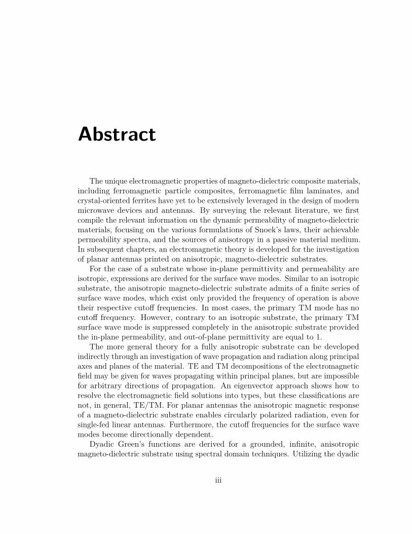
The unique electromagnetic properties of magneto-dielectric composite materials,including ferromagnetic particle composites, ferromagnetic film laminates, andcrystal-oriented ferrites have yet to be extensively leveraged in the design of modernmicrowave devices and antennas. By surveying the relevant literature, we firstcompile the relevant information on the dynamic permeability of magneto-dielectricmaterials, focusing on the various formulations of Snoek’s laws, their achievablepermeability spectra, and the sources of anisotropy in a passive material medium.In subsequent chapters, an electromagnetic theory is developed for the investigationof planar antennas printed on anisotropic, magneto-dielectric substrates.

For the case of a substrate whose in-plane permittivity and permeability areisotropic, expressions are derived for the surface wave modes. Similar to an isotropicsubstrate, the anisotropic magneto-dielectric substrate admits of a finite series ofsurface wave modes, which exist only provided the frequency of operation is abovetheir respective cutoff frequencies. In most cases, the primary TM mode has nocutoff frequency. However, contrary to an isotropic substrate, the primary TMsurface wave mode is suppressed completely in the anisotropic substrate providedthe in-plane permeability, and out-of-plane permittivity are equal to 1.

The more general theory for a fully anisotropic substrate can be developedindirectly through an investigation of wave propagation and radiation along principalaxes and planes of the material. TE and TM decompositions of the electromagneticfield may be given for waves propagating within principal planes, but are impossiblefor arbitrary directions of propagation. An eigenvector approach shows how toresolve the electromagnetic field solutions into types, but these classifications arenot, in general, TE/TM. For planar antennas the anisotropic magnetic responseof a magneto-dielectric substrate enables circularly polarized radiation, even forsingle-fed linear antennas. Furthermore, the cutoff frequencies for the surface wavemodes become directionally dependent.

Dyadic Green’s functions are derived for a grounded, infinite, anisotropicmagneto-dielectric substrate using spectral domain techniques. Utilizing the dyadic

iii

Green’s functions, the surface wave excitations and radiation patterns of shortelectric dipole antennas are calculated. The principal plane patterns for a dipoleover a substrate possessing in-plane anisotropy are also derived. A method ofmoments computer program is developed for the numerical investigation of theinput impedance and efficiency of microstrip dipoles printed over an anisotropicmagneto-dielectric substrate. Example results are given to illustrate the effect ofthe anisotropic properties of the magneto-dielectric substrate on the dipole’s reso-nant length, impedance, and efficiency. Notably, the results indicate that a higherefficiency is obtained if the permittivity of the substrate in the direction normal tothe air-substrate interface is small, an effect attributable to the suppression of theprimary TM surface wave mode.

From these results, we also conclude that the permeability in the directionnormal to the air-substrate interface is unimportant for thin substrates. Conse-quently, no penalty is paid for utilizing anisotropic magnetic materials such asthe crystal-oriented ferrites, which only possess an in-plane permeability. Thesuperior frequency-permeability Snoek product of the oriented magnetic materialscompared to traditional isotropic materials, combined with the unimportance of theout-of-plane permeability, lead to the conclusion that anisotropic magneto-dielectricmaterials are potentially better-suited for antenna applications than their isotropiccounterparts.

iv

Table of Contents

List of Figures viii

Acknowledgments xi

Chapter 1Overview and Introduction 11.1 Overview of Prior Studies on the Application of Magnetic Materials

to Antenna Design . . . . . . . . . . . . . . . . . . . . . . . . . . . 31.2 Contributions to Knowledge . . . . . . . . . . . . . . . . . . . . . . 71.3 The Layout of this Dissertation . . . . . . . . . . . . . . . . . . . . 9

Chapter 2Permeability of Anisotropic Magnetic Materials 102.1 Ferromagnetism from Magnetic Domain Rotation . . . . . . . . . . 11

2.1.1 Equation of Motion for Internal Magnetization . . . . . . . . 132.1.2 Easy-Plane Crystalline Anisotropy and Demagnetization Fields 18

2.2 Crystal-Oriented Ferrites . . . . . . . . . . . . . . . . . . . . . . . . 242.3 Ferromagnetic Laminates . . . . . . . . . . . . . . . . . . . . . . . . 382.4 Ferromagnetic Particle Composites . . . . . . . . . . . . . . . . . . 42

Chapter 3Electromagnetic Wave Propagation in Anisotropic Magneto-

dielectric Media 483.1 Maxwell’s Equations in Anisotropic Media . . . . . . . . . . . . . . 493.2 Plane Wave Solutions . . . . . . . . . . . . . . . . . . . . . . . . . . 52

3.2.1 TEM Wave Propagation Along Principal Axes . . . . . . . . 533.2.2 TE and TM Wave Propagation Within Principal Planes . . 563.2.3 TE and TM Wave Propagation in Arbitrary Directions For

Magneto-dielectric Medium With In-Plane Isotropy . . . . . 59

v

3.2.4 Hybrid Mode Wave Propagation for Arbitrary Directions ofPropagation . . . . . . . . . . . . . . . . . . . . . . . . . . . 65

3.3 Surface Wave Modes of the Grounded Substrate . . . . . . . . . . . 683.3.1 Surface Waves in Substrates with In-Plane Isotropy . . . . . 693.3.2 TE and TM Surface Wave Propagation Within Principal

Planes . . . . . . . . . . . . . . . . . . . . . . . . . . . . . . 74

Chapter 4Electromagnetic Radiation in the Presence of an Anisotropic

Magneto-dielectric Substrate 774.1 The Plane Wave Spectrum, and Formulation of the Green’s Function

Problem . . . . . . . . . . . . . . . . . . . . . . . . . . . . . . . . . 794.2 Dyadic Green’s Functions for Substrate with In-Plane Isotropy . . . 82

4.2.1 Asymptotic Evaluation of the Radiation Field by StationaryPhase . . . . . . . . . . . . . . . . . . . . . . . . . . . . . . 87

4.2.2 Excitation of Surface Waves . . . . . . . . . . . . . . . . . . 924.3 Radiation over a Generally Anisotropic Substrate . . . . . . . . . . 101

4.3.1 Necessary Conditions for the Excitation of Circularly Polar-ized Radiation Fields . . . . . . . . . . . . . . . . . . . . . . 103

4.3.2 Principal Plane Radiation . . . . . . . . . . . . . . . . . . . 105

Chapter 5Method of Moments Analysis of Microstrip Dipoles 1085.1 Spectral Formulation of the Electric-Field Integral Equation . . . . 1085.2 Basis Functions and Source Model . . . . . . . . . . . . . . . . . . . 1115.3 Numerical Integration . . . . . . . . . . . . . . . . . . . . . . . . . 1135.4 Input Impedance Analysis . . . . . . . . . . . . . . . . . . . . . . . 1165.5 Anisotropic Effects . . . . . . . . . . . . . . . . . . . . . . . . . . . 124

Chapter 6Conlusions and Future Work 128

Bibliography 132

Appendix AThe Spectral Dyadic Green’s Function in the Complex Plane 138

Appendix BMethod of Moments MATLAB Code 141

vi

Appendix CComparisons to FEKO for an Isotropic Substrate 149

vii

List of Figures

2.1 A magnetic specimen is divided up into domains with disorderedorientations in the absence of an external magnetic field. . . . . . . 12

2.2 A uniformly magnetized sphere. . . . . . . . . . . . . . . . . . . . . 202.3 A uniformly magnetized infinite slab. . . . . . . . . . . . . . . . . . 212.4 A boundary value problem for the change in permeability due to a

small embedded magnetic domain. . . . . . . . . . . . . . . . . . . . 272.5 Curve fits to measured permeability of Nickel ferrites [36]. Solid and

dashed lines of matching colors represent the real and imaginaryparts, respectively, of the permeability for a particular Nickel ferritesample of density d. For the imaginary permeability, − Im(µg) isplotted so that only positive values are needed for the vertical axis. 32

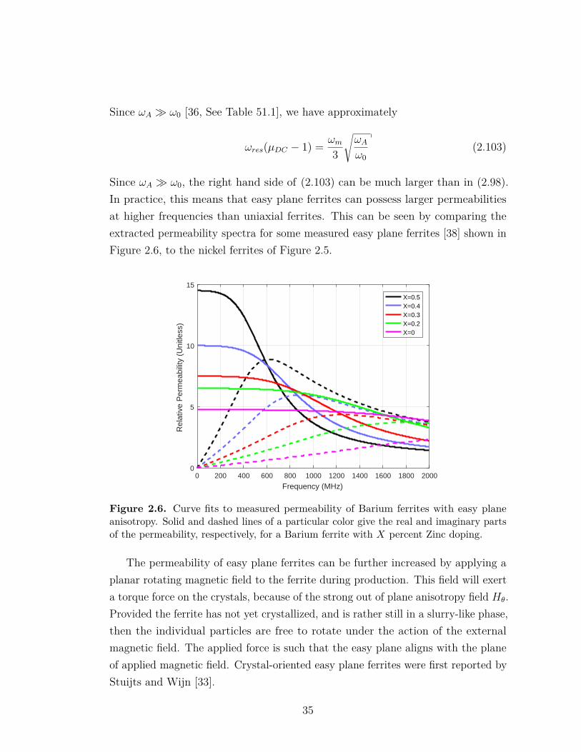
2.6 Curve fits to measured permeability of Barium ferrites with easyplane anisotropy. Solid and dashed lines of a particular color givethe real and imaginary parts of the permeability, respectively, for aBarium ferrite with X percent Zinc doping. . . . . . . . . . . . . . 35

2.7 Fitted curves for the in-plane permeability of crystal-oriented easyplane ferrites. The solid and dashed lines of a particular colorcorrespond to the real and imaginary permeabilities of a particularferrite. The sources for the data are indicated in the legend. . . . . 37

2.8 The directional permeabilities of a crystal-oriented easy plane fer-rite [30]. Black and red curves are the in-plane and out-of-planedirectional permeability, respectively. Solid and dashed lines are thereal and imaginary parts, respectively. . . . . . . . . . . . . . . . . 38

2.9 A biphasic composite material. . . . . . . . . . . . . . . . . . . . . 392.10 A curve fit to the measured permeability spectrum along the in-plane

hard axis of a ferromagnetic laminate of single domain films [42]. . . 422.11 The spheroid viewed along z (left panel) and along y (right panel). 432.12 Comparison of spherical particle permeability and effective perme-

ability at 45% particle concentration. . . . . . . . . . . . . . . . . . 46

viii

3.1 The geometry of a TM plane wave in anisotropic magneto-dielectricmedia. In the figure, ψ < π/2, hence the medium depicted must haveεz > εt. If instead, ψ > π/2, then εz < εt. . . . . . . . . . . . . . . . 64

3.2 Propagation coefficients of complex waves versus the free spacewavenumber. . . . . . . . . . . . . . . . . . . . . . . . . . . . . . . . 68

3.3 Anisotropic magneto-dielectric Substrate Geometry. . . . . . . . . . 683.4 Electric field lines for the TM0 surface wave mode in an anisotropic

magneto-dielectric substrate. The field lines pictured are obtainedby the choice of parameters: εt = 5 ; εz = 6 ; µt = 10 ; k0 = 2π ;h = .02. . . . . . . . . . . . . . . . . . . . . . . . . . . . . . . . . . 73

3.5 Magnetic field lines for the TE0 surface wave mode in an anisotropicmagneto-dielectric substrate. The field lines pictured are obtainedfor: εx = 10 ; µz = 6 ; µy = 5 ; k0 = 4π ; h = .02. . . . . . . . . . . 76

4.1 Source-Excited magneto-dielectric Antenna Substrate. . . . . . . . . 804.2 Polar plots of the E-plane (blue traces) and H-plane (red traces)

electric field patterns of a short dipole over thin substrates. Theradial magnitude axis is in logarithmic units, and normalized to 0dB. All plots are computed with a thin substrate with h = .05 λ√

µtεt.

Panels (a) and (b) show that µz has no effect. Panels (c) and (d)show the influence of εz in a non-magnetic thin substrate. Panels (e)and (f) show that εz has no influence on patterns when the substrateis strongly magnetic. . . . . . . . . . . . . . . . . . . . . . . . . . . 93

4.3 Polar plots of the E-plane (blue traces) and H-plane (red traces)electric field patterns of a short dipole over thick substrates. Plotsare computed setting h = .5 λ√

µtεt. . . . . . . . . . . . . . . . . . . . 94

4.4 Original contour C1 from −∞ to +∞, and contour C2 deformedaround branch cut for kz1 . During the contour deformation, thesurface wave pole at ktp is crossed. . . . . . . . . . . . . . . . . . . . 97

4.5 Contours for integration of radiated and total power. In the figure,km is defined as max

(k0√µtεz , k0

√εtµz

). . . . . . . . . . . . . . . 101

4.6 Efficiency of short dipoles versus substrate thickness and electromag-netic properties. Cusps on plots are indicative of crossing a cutoffpoint for a higher order surface wave mode. . . . . . . . . . . . . . 102

5.1 Overlapping triangular subdomain basis functions. . . . . . . . . . . 1125.2 Integration contour for calculation of Zmn. . . . . . . . . . . . . . . 1155.3 Input impedance versus length for a microstrip dipole. For this

calculation, W = 0.01λ0, ε = 2.45I, µ = I, and h = 0.2λ0. Notethat W and h are rescaled at each value for the length. . . . . . . . 117

ix

5.4 Resonant length of microstrip dipoles versus the permittivity of anisotropic substrate. For this calculation, W = 0.01λ0, ε = εrI, µ = I,and h = 0.2λ0. . . . . . . . . . . . . . . . . . . . . . . . . . . . . . . 118

5.5 Resonant length of microstrip dipoles versus the permeability of anisotropic substrate. For this calculation, W = 0.001λ0, ε = I, andh = 0.2λ0. . . . . . . . . . . . . . . . . . . . . . . . . . . . . . . . . 119

5.6 Input impedance versus length for a microstrip dipole over a magneto-dielectric substrate with εr = 3 and µr = 50 and W = h = L/12.5. . 120

5.7 VSWR versus length for a microstrip dipole over a magneto-dielectricsubstrate with εr = 3 and µr = 50 and W = h = L/12.5. . . . . . . 120

5.8 Efficiency of the microstrip dipole lying over a substrate with µr = 50and εr = 3. . . . . . . . . . . . . . . . . . . . . . . . . . . . . . . . 123

5.9 Comparison of input impedance of microstrip dipoles with andwithout dielectric anisotropy. We set W = 0.01λ0 and h = 0.1λ0. . . 125

5.10 Comparison of efficiency of microstrip dipoles with and withoutdielectric anisotropy. We set W = 0.01λ0 and h = 0.1λ0. . . . . . . 126

5.11 Comparison of directive gain with and without dielectric anisotropy. 127

A.1 Branch cuts for kz1 (given by dashed red lines). . . . . . . . . . . . 140

C.1 Input impedance, comparison of our model to FEKO. . . . . . . . . 150C.2 Directive gain, comparison of our model to FEKO. . . . . . . . . . 150C.3 Segmentation of the microstrip dipole in FEKO. . . . . . . . . . . . 151

x

Acknowledgments

This research was made possible by the Walker graduate assistantship programat the Penn State Applied Research Laboratory, and the Brown Graduate andSociety PS Electrical Engineering Fellowships.

My sincerest thanks are owed to my advisor Dr. James Breakall for his willing-ness to oversee the completion of my research. His advisory approach involved aminimum of distractions, and allowed the work to be completed in a timely fashion.I would also like to thank Dr. Steven Weiss, for encouraging me to pursue a doctoraldegree, and for introducing me to many of the mathematical techniques that makethis research possible. I offer additional thanks to my committee members Dr. JulioUrbina, Dr. Victor Pasko, and Dr. Michael Lanagan for constructive suggestionsfor improving this dissertation.

I am grateful to my parents for their consistently wise advice, and for encouragingme to pursue a career in engineering. Lastly, I would like to acknowledge the lovingsupport of my wife Theresa. Her confidence in me has never waivered. Mostamazingly, during the last six months, she took upon the task of caring for ournewborn son through the night, allowing me to dedicate the time fully to writing.

xi

Dedication

For my wife Theresa and son Levi.

xii

Chapter 1 |Overview and Introduction

The incorporation of exotic materials into antenna designs remains a frontier forinteresting theoretical research. The most general linear material is the bianisotropicmedium, which requires 36 different constitutive parameters to specify completely.Under the conditions of reciprocity, 16 of the 36 parameters are independent [1]. Ifelectromagnetic chiral materials are excluded, and a coordinate system is chosen tobe aligned with the material’s 3 principal axes, then only 6 parameters remain [2, pp.110-111]. The specification of these parameters defines the anisotropic magneto-dielectric material. In an anisotropic magneto-dielectric we presume the materialmay be described by permittivity and permeability tensors of the form

µ = xxµx + yyµy + zzµz (1.1)

ε = xxεx + yyεy + zzεz (1.2)

the main assumption being that both the magnetic and dielectric principal axes arealigned with the same set of Cartesian coordinate axes x, y, and z. Empirical dataseems to support this assumption. For instance, see [3]. In Chapter 2, we discussthe sources of anisotropy in the permeability tensor for ferromagnetic materials.

It is now well-established that antennas built with high-permittivity dielectricsexhibit poor impedance bandwidth [4]. This is due, in part, to the inherent sizereductions, which can be associated through Chu’s theory [5] with a higher radiationQ factor. We might expect the introduction of a high permeability (instead ofpermittivity) would offer no advantage. After all, we often still expect a sizereduction. However, in many cases, a large permeability implies fundamentallydifferent behavior than a large permittivity. For example, consider that the sign on

1

the reflection coefficient for normally incident plane waves on a magnetic materialis positive, not negative as is the case for a dielectric material. Furthermore, theasymptotic behavior of a magnetic material as µr →∞ is that of a perfect magneticconductor (PMC). From image theory, an antenna positioned over a PMC groundplane can be placed arbitrarily close to the ground plane, thus minimizing thephysical space required by the antenna. Moreover, the resonant length of a dipoleover a PMC ground plane is still approximately λ0/2. Thus, in actuality, theintroduction of permeability need not necessarily result in a size reduction along aphysical dimension that would impact bandwidth.

As we will show in Chapter 4, a magnetic ground plane with large values of µrwill possess excellent wave-trapping capability. In fact, its wave trapping capabilityfar exceeds a non-magnetic substrate with an equivalent value of permittivity. Thus,a planar antenna positioned over a magnetic substrate will usually deliver a largepercentage of its power into trapped surface waves in the substrate, which leads tolow efficiency. It would seem that materials with comparable values of permittivityand permeability are the best bet. The behavior of an antenna positioned over asubstrate with arbitrary values of permittivity and permeability, though, is verydifficult to predict from intuition alone. Precise models need to be formulated, andnumerical analysis needs to be conducted.

We may add additional degrees of freedom by allowing the material’s permittivityand permeability to vary over different directions. As will be demonstrated inChapter 2 of this dissertation, a large class of materials is obtainable that possessesanisotropic magnetic properties. One of the principal conclusions of this researchis that the anisotropic magnetic materials are potentially better suited for planarantenna designs than their isotropic counterparts.

We can enumerate at least 2 advantages of using anisotropic magnetic materials.The first and most important relates to Snoek’s law. We review in Chapter 2,why anisotropic magnetic materials inherently possess a larger Snoek product,and consequently why they can possess a greater value of permeability at higherfrequencies, than their isotropic counterparts. For thin magnetic substrates, we alsoshow in Chapter 5 that the permeability normal to the air-substrate interface is notimportant. Thus, if we sacrifice permeability in the normal direction in exchangefor a larger Snoek product for the in-plane permeability, we are getting all theintended benefit without any downside. Hence, if for no other reason, anisotropic

2

magnetic materials are preferable.Another intriguing possibility involves the application of anisotropy in the

permittivity of a material. It is shown, for instance, in Chapter 3 that the primaryTM surface wave mode cannot propagate if the in-plane permeability and normalpermittivity are equal to 1. Subsequently, in Chapter 5, we show that even forsmaller values of the normally directed permittivity, that the primary TM surfacewave is suppressed to a degree, leading to improved efficiency of planar antennas asradiators.

Our principal contribution is in the development of precise electromagneticmodels that include a general form of magneto-dielectric anisotropy. Since the searchfor effective antenna designs now invariably involves some amount of optimization,formulating precise numerical models incorporating new degrees of freedom hasbecome an essential component of theoretical progress in the field of antennas.

1.1 Overview of Prior Studies on the Application ofMagnetic Materials to Antenna Design

The most popular and prevalent antenna that makes use of magnetic materialshas to be the ferrite rod or “loopstick” antenna. The design calls for many turnsof wire coiled around a cylindrical ferrite core. The resultant antenna possesses aradiation resistance that far surpasses a simple small dipole of a comparable size,and is easily more efficient [6]. However, the antenna is still much less efficientthan an actual resonant dipole of the appropriate half-wavelength size. Moreover,the nonlinear nature of the magnetic material is such that it can only presenta permeability to fields of a relatively small magnitude. The nonlinear naturethus makes the antenna unsuitable for use in a broadcast station requiring largetransmission power. In a low-frequency channel where low-profile, low cost mobilereceivers are desired, an electrically small ferrite rod antenna that is as efficient aspossible, though still not very efficient, is acceptable, especially since the differencecan be made up by increasing transmission power and using a physically largeantenna at the central transmitting station. Indeed, the ferrite rod antenna is incommon use for mobile AM radio receivers.

There are other applications, in higher frequency bands, where similar require-

3

ments would suggest we look again to magnetic materials for solutions that admitof similar tradeoffs. Moreover, if the application does not call for an extremelylarge amount of transmit power, then a magnetic material antenna solution canbe considered also for transmission. In the remainder of this section, we considersome instances of antennas designed with magnetic materials that have appearedin the literature.

An important distinction that must be made, is whether the magnetic materialis operated with or without an applied variable DC magnetic field bias. With amagnetic field bias applied to a ferrite or other ferromagnetic material, its propertieschange with the amplitude and direction of the applied bias. Furthermore, wavepropagation becomes nonreciprocal, and the permeability matrix must containnonzero off-diagonal entries, making analysis difficult. Several publications existtreating the biased ferrite substrate for patch and microstrip antenna geometries [7][8] [9] [10]. It has been demonstrated in these investigations, often experimentally,that the biasing of the ferrite enables some control over the various characteristicsof antennas, including the beam direction, resonance frequency, and principlepolarization. As a consequence of non-reciprocity, an antenna with different transmitand receive radiation patterns is possible [10].

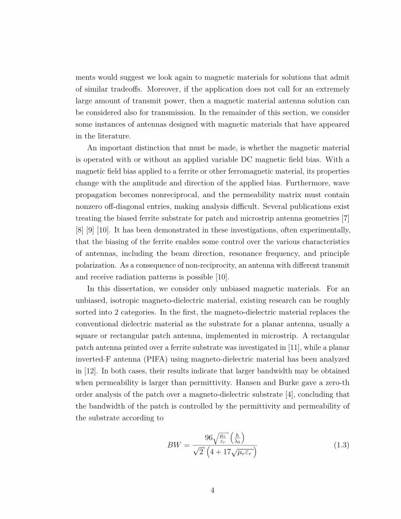
In this dissertation, we consider only unbiased magnetic materials. For anunbiased, isotropic magneto-dielectric material, existing research can be roughlysorted into 2 categories. In the first, the magneto-dielectric material replaces theconventional dielectric material as the substrate for a planar antenna, usually asquare or rectangular patch antenna, implemented in microstrip. A rectangularpatch antenna printed over a ferrite substrate was investigated in [11], while a planarinverted-F antenna (PIFA) using magneto-dielectric material has been analyzedin [12]. In both cases, their results indicate that larger bandwidth may be obtainedwhen permeability is larger than permittivity. Hansen and Burke gave a zero-thorder analysis of the patch over a magneto-dielectric substrate [4], concluding thatthe bandwidth of the patch is controlled by the permittivity and permeability ofthe substrate according to

BW =96√

µr

εr

(hλ0

)√

2(4 + 17√µrεr

) (1.3)

4

A main result of this formula, as discussed in the paper, is that for a small √εrµr ,the bandwidth of a patch printed over a εr = µr substrate is roughly the same asthe bandwidth of the patch situated over the corresponding dielectric substratewhere the permittivity is still εr but the permeability is µr = 1. Yet, the resonantlength is reduced by a factor of √µr . Thus an additional size reduction factorcould theoretically be achieved without paying an additional bandwidth penalty.

The second primary utilization of a magneto-dielectric material is as a coatingon an antenna’s conductive backplane. In this case, the antenna is not printeddirectly over a substrate lying over the ground plane. Instead, there is a certainamount of free space between the antenna element and the ground plane. Normally,this distance is required to be large to avoid poor behavior, as the image currentsthrough the backplane tend to cancel the radiation. With the magneto-dielectriccoating, it is reasoned, the reflection of the impinging radiation from the antennaelement will be associated with a reflection coefficient of a positive sign. Thus, thereturning radiation need not, in theory, pose any substantive problems in terms ofthe input impedance, even as the antenna element is subsequently brought veryclose to the ground plane. For instance, Breakall designed a broadband planardipole antenna positioned over a magneto-dielectric-coated ground plane, thatexhibited a decreased spatial profile [13]. A similar design for a planar archimedeanspiral over a magneto-dielectric-coated ground plane has been considered by otherresearchers [14]. For the archimedean spiral, the magnetic material was chosen tosatisfy µr = εr, and to be lossy. Thus, their intention was apparently to use thecoating as an absorber, and to take the 3 dB hit to directive gain in the forwarddirection, in exchange for an antenna with a low spatial profile exhibiting largebandwidth.

Comparatively less has been written on the use of anisotropic magneto-dielectricmaterials in antennas, though, several antenna designs have been reported. Aninteresting antenna developed by Metamaterials, Inc., and reported by Mitchelland Weiss, utilizes several designed anisotropic magneto-dielectric materials withvarying values of permeability and permittivity along different directions [3]. Thelarge permeability of the materials along certain axes is leveraged, by orientingseveral material samples under the various arms of a planar crossed dipole accordingto the local direction of the magnetic field generated by the currents flowing on theantenna. For each material sample, a significant permeability is exhibited along

5

one axis only. Thus this axis is aligned with the anticipated direction along whichthe magnetic field should have the largest magnitude. The two arms of the crosseddipole are loaded with disparate magneto-dielectric materials, designed to achieve arelative phasing between the radiated fields from the arms, which enables circularlypolarized radiation to be obtained.

A separate antenna concept has been reported by Mitchell [3]. In his work, aresonant cavity is loaded at a chosen location with an anisotropic magneto-dielectricmaterial. The cavity has a slot cut into it, turning the cavity into an antennawhose properties are perturbed by the presence of the magneto-dielectric materialloading. An anisotropic transverse resonance theory is proposed to explain theantenna’s functioning, and is supported by calculations using the Finite DifferenceTime Domain (FDTD) method.

Our analysis for the anisotropic magneto-dielectric substrate is modeled, inpart, after the analogous treatments that have been given for anisotropic dielectricsubstrates. For instance, a numerical analysis of a patch printed on an anisotropicdielectric (µr = 1) substrate has been conducted by Pozar [15]. His analysisshows that the permittivity along the in-plane and out-of-plane directions exertvarious influences on the resonant length of the patch. A general matrix-eigenvectortheoretical method is given by Krowne for the derivation of Green’s functions forgeometries involving anisotropic layered materials [16].1 Based on Krowne’s work,more detailed numerical analyses have been given for anisotropic dielectric substrateswith arbitrary alignment of its principal axes by Pettis and Graham [17] [18]. Thesestudies demonstrated further, that the resonant lengths, radiation patterns, andinput impedance of microstrip dipoles and patches are influenced by the anisotropy.

In our opinion, the most serious gaps in understanding the properties of planarantennas printed over anisotropic magneto-dielectric substrates arise from a lack ofknown results regarding the surface wave modes. For instance, little is currentlypublished regarding the cutoff frequencies, or mode patterns, for surface wavespropagating in an anisotropic substrate. This information is critical to under-standing the dependence of the surface waves on the substrate anisotropy. Thesurface wave excitation of a substrate is a principle cause of low efficiency in planarantennas, and moreover, is responsible for degradational effects associated with

1The theoretical formulation given in Chapter 3 of this disseration makes similar use ofeigenvectors as suggested by Krowne.

6

surface-wave-mediated mutual coupling between elements functioning within anantenna array. A primary goal of this dissertation is to integrate a treatment ofthe surface waves (in the anisotropic substrate), into a more complete analysis ofplanar printed antennas. Our analysis will enable some conclusions to be drawn,regarding what our preferences should be for the properties of magneto-dielectricmaterials intended for use in planar antenna design.

1.2 Contributions to KnowledgeThe novel contributions of this dissertation are contained primarily in the

theoretical explorations of surface wave propagation in the anisotropic magneto-dielectric substrate, and its role in controlling the efficiency and gain of printedmicrostrip dipole antennas. Several publications have resulted from research relatedto the composition of this disseration. An Army Research Laboratory technicalreport [19], and two theoretical papers have been published concerning the solutionof electromagnetic boundary value problems [20] [21]. A paper concerning themethod of moments analysis of microstrip dipoles printed on anisotropic magneto-dielectric substrates, as discussed in Chapter 5, is in preparation [22]. While thetopic is not treated here, from the author’s research on magneto-dielectric media,attention was drawn to work on refraction through periodic media comprisingdensely spaced magneto-dielectric spheres, resulting in a paper on the theoreticalexplanation for negative refraction [23].

In this dissertation, the following results are developed:

• Snoek’s laws are derived for uniaxial ferrites, easy-plane ferrites, ferromagneticlaminates, and ferromagnetic particle composites.

• A new derivation is given for the permeability tensor of a magnetic domainfor a ferrite with easy-plane crystalline anisotropy.

• A concise eigenvector formulation is developed for the plane-wave solutionsof Maxwell’s equations in an anisotropic magneto-dielectric medium.

• Analytical expressions are derived for the trapped surface wave modes in amagneto-dielectric substrate with in-plane isotropy. Inequalities bounding

7

the propagation coefficients, formulas for the cutoff frequencies, and field lineplots for the modal profiles are provided.

• From the bounding inequalities for the surface wave propagation, it is proventhat the primary TM surface wave can be suppressed in a substrate for acertain choice of directional permittivity and permeability.

• Dyadic Green’s functions are found for the calculation of the electromagneticfields due to impressed surface current distributions lying over an anisotropicmagneto-dielectric substrate.

• The far-field radiation formulas are utilized to prove that circularly polarizedradiation may be obtained from a linearly-polarized current distribution, suchas that supported by a single-feed microstrip dipole, by exploiting in-planeanisotropy in a magneto-dielectric substrate.

• A method of moments algorithm is given, along with the computer programin an appendix, for the calculation of the current distribution on a center-fed microstrip dipole printed over an anisotropic magneto-dielectric antennasubstrate. The algorithm calculates input impedance, efficiency, and directivegain, and includes provisions checking that the solutions satisfy Poynting’stheorem.

• From a method of moments analysis of microstrip dipoles, it is shown thathighly permeable substrates effect tradeoffs in an antenna design betweenefficiency and bandwidth.

• An argument is developed, and supported by numerical results, that magneticanisotropy may be disregarded in the case of an in-plane isotropic material.Consequently, anisotropic materials may be utilized where the out-of-planepermeability is equal to 1, without affecting performance.

• Numerical results are given, which show that the efficiency of microstripdipoles may be improved by controlling the dielectric anisotropy of thesubstrate. This effect is attributed to the suppression of the transversemagnetic (TM) surface wave.

8

1.3 The Layout of this DissertationIn Chapter 2, we investigate known information regarding passive anisotropic

properties of magnetic materials, including crystal-oriented ferrites, ferromagneticlaminates, and particle composites. The various Snoek’s laws are derived, andfrom the models for the permeability spectra, extracted best-fit curves of measuredpermeability spectra are shown. In Chapter 3, the analytic expressions for surfacewave modes are developed starting from Maxwell’s equations. An analysis ofthe surface wave modes’ cutoff frequencies, and plots of their modal profiles aregiven. In Chapter 4, dyadic Green’s functions are introduced, and from them, theradiation patterns of short dipoles are calculated. Starting from the dyadic Green’sfunction, the surface wave excitations by a short dipole are also analyzed in thecomplex plane, and the efficiency, defined as the proportion of power delivered tothe radiation field versus the total power (which includes surface wave power), iscalculated for various values of permittivity and permeability along the in-plane andout-of-plane directions. In Chapter 5, a method of moments algorithm is detailedfor the solution of the currents on a microstrip dipole positioned over the anisotropicmagneto-dielectric substrate. A method is given for the separate calculation ofradiated and surface wave power, so that efficiencies can be compared for variousvalues of the substrate properties. In Appendix A, we give an explanation of thecomplex square roots appearing in the dyadic Green’s function. A code listingfor the method of moments MATLAB program is given in Appendix B. Finally,validation of the MATLAB program against commercially available software, forthe restricted case of an isotropic substrate, is given in Appendix C.

In this dissertation, ejωt time variation is assumed. Vectors are written in boldfont. Unit vectors are indicated with a hat, as in a. Dyadic/matrix quantities aredenoted using a double over-bar, as in A. Square brackets are reserved mainly for

matrices, such asA B

C D

. SI units are used throughout the dissertation.

9

Chapter 2 |Permeability of AnisotropicMagnetic Materials

In Chapters 3 and 4 we study electromagnetic propagation and radiation of wavesin anisotropic magneto-dielectric substrates. In this chapter, we focus specificallyon the permeability tensor. The goal of this chapter is to establish that a largeclass of materials is obtainable, that for a proper model of electromagnetic wavepropagation to be given, requires we assign a permeability tensor to the material ofthe general form

µ = xxµx + yyµy + zzµz (2.1)

While it is possible to produce artificially magnetic substrates utilizing effectivemedium techniques [24], the resulting magnetic properties are weak at low frequency,and highly dispersive at frequencies where the magnetic properties are strong. Wefocus instead on naturally ferromagnetic materials. In order to understand the pos-sibilities and limitations inherent in working with ferromagnetic materials, we givea treatment in this chapter of the dynamic permeability tensor of macroscopicallyanisotropic magnetic materials.

We describe the theory for the gyromagnetic response of magnetic domainsto external magnetic fields in Section 2.1. We consider the effects of crystallineanisotropy fields, in both uniaxial and easy-plane crystals. We also incorporatedemagnetization fields arising from the finite boundaries of the domain. In Section2.2, we then discuss how the anisotropy fields lead to macroscopically anisotropicpermeability in crystal-oriented ferrites. In Sections 2.3 and 2.4, we discuss howuniaxial crystalline anisotropy, and demagnetization fields lead to anisotropic

10

permeability in ferromagnetic-laminate and particle composites.By its very nature, this review must borrow heavily from existing literature on

magnetic materials. Our intention is to give a reasonably self-contained treatment,at a theoretical level appropriate for the curious antenna engineer, who would likea basic grasp of the achievable properties of magnetic materials, and especially toknow their fundamental limitations.

We do not consider the incremental permeability of materials that are ina remanent magnetized state. Additionally, we assume that materials are notsubjected to an active DC magnetic field bias. Moreover, although eddy currentsplay an important role in placing additional limits on the obtainable performanceof certain magnetic materials, particularly the laminate and particle composites,we omit its consideration here, for simplicity. We also use the word ferromagneticin a wider sense than is now usual, and take it to include both metallic alloys of Ni,Co, and Fe, and ferrimagnetic materials, such as ferrites.

2.1 Ferromagnetism fromMagnetic Domain RotationFerromagnetic materials are a rather small class constituting only several ele-

ments in pure form and some of their compounds. In fact, at room temperature,and in pure chemical form, only Ni, Fe, and Co are ferromagnetic [25]. At lowertemperatures, other elements become ferromagnetic, including several elementsfrom the lanthanide series of the periodic table [25]. Metal alloys and certain oxidesof these and other elements are also ferromagnetic. The various oxides of Ni, Fe, andCo are collectively referred to as ferrites. The addition of non-metallic elements intothe crystal structure of ferrites endows them with low electrical conductivity, andconsequently, ferrites have found more widespread use in electromagnetic devicesoperating at microwave frequencies.

All materials respond to externally applied magnetic fields, but in most situationscommon to our everyday experience, these responses are small and inconsequential.In a paramagnetic material, electron spins experience a torque force that tendsto reorient their magnetic dipole moments toward external fields. However, eachelectron responds more or less independently to the magnetic field. The force ona single isolated electron is small, and the tendency of this force to reorient theelectron spin magnetic moment is easily nullified by thermal vibrations.

11

A ferromagnetic material also derives its magnetic response from the spin mag-netic moment of the electron. However, the ferromagnetic material is uniquelycharacterized by the existence of a strong coupling force of quantum mechanicalorigins. This force tends to spontaneously align magnetic spin moments of neighbor-ing electrons. Coupled electrons behave like coherent magnetic dipoles with largermagnetic moments. The torque force exerted upon the larger magnetic momentscan overcome the quashing effect of thermal vibrations.

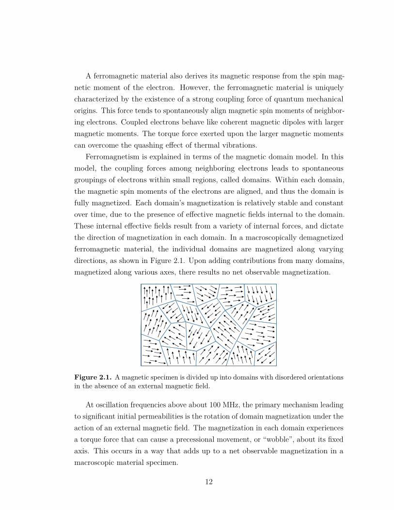
Ferromagnetism is explained in terms of the magnetic domain model. In thismodel, the coupling forces among neighboring electrons leads to spontaneousgroupings of electrons within small regions, called domains. Within each domain,the magnetic spin moments of the electrons are aligned, and thus the domain isfully magnetized. Each domain’s magnetization is relatively stable and constantover time, due to the presence of effective magnetic fields internal to the domain.These internal effective fields result from a variety of internal forces, and dictatethe direction of magnetization in each domain. In a macroscopically demagnetizedferromagnetic material, the individual domains are magnetized along varyingdirections, as shown in Figure 2.1. Upon adding contributions from many domains,magnetized along various axes, there results no net observable magnetization.

Figure 2.1. A magnetic specimen is divided up into domains with disordered orientationsin the absence of an external magnetic field.

At oscillation frequencies above about 100 MHz, the primary mechanism leadingto significant initial permeabilities is the rotation of domain magnetization under theaction of an external magnetic field. The magnetization in each domain experiencesa torque force that can cause a precessional movement, or “wobble”, about its fixedaxis. This occurs in a way that adds up to a net observable magnetization in amacroscopic material specimen.

12

2.1.1 Equation of Motion for Internal Magnetization

A basic understanding of ferromagnetism starts with a consideration of themagnetic response of a domain to an external oscillating magnetic field. Since eachdomain is composed of individual magnetic dipoles arising from the spin momentsof electrons, we begin by considering the force felt by the electron in an appliedmagnetic field B.

If we treat the electron classically like a distributed sphere of charge spinningon its axis, we would obtain for its spin magnetic dipole moment,

m = − eL2me

(2.2)

where e is the charge of an electron, and me is its mass. L is the vector angularmomentum of the electron’s spin, which in a classical description would be given by

L = zIω0 (2.3)

where I is the electron’s rotational inertia and ω0 its angular velocity. Quantummechanics, however, shows that the true spin magnetic moment of an electrondeviates from this classical prediction by a constant of proportionality termed theLandé factor g [25],

m = − ge

2me

L (2.4)

The ratio of the spin magnetic moment to the angular momentum is termed thegyromagnetic ratio γ.

γ = ge

2me

≈ 1.76086× 1011 (s · T)−1 (2.5)

If the electron is exposed to a uniform static magnetic field B, a torque force isproduced given by

T = m×B (2.6)

This torque force acts on the angular momentum of the electron according to theclassical equation of motion for the rotation of a rigid body [26]

T = dLdt

(2.7)

13

Combining (2.4)-(2.7), we obtain

dmdt

= −γm×B (2.8)

Magnetic domains consist of many coupled electrons contributing aligned magneticdipole moments mk. The number of atoms in each domain varies, but is oftenon the order of 1015 or 1016 atoms [2]. It is therefore permissible to treat eachmagnetic domain as a continuous distribution of magnetic dipole moment density.Thus, we define a magnetization density vector [2]

M = lim∆v→0

n∆v∑k=1

mk

(∆v) (2.9)

and let (2.8) pass in this limit to the vector point relation

dMdt

= −γM×B (2.10)

By definition, the magnetic field vectors B and H existing within the magneticdomain relate to this magnetization according to

B = µ0(H + M) (2.11)

where µ0 = 4π · 10−7 (H/m) is the permeability of free space. We find, uponsubstituting (2.11) into (2.10), and noting that M×M = 0,

dMdt

= −γµ0M×H (2.12)

which is an equation of motion for the magnetization within an isolated domain.In order to utilize (2.12) to investigate dynamic magnetization responses, it is

necessary to make assumptions regarding the static components of magnetizationand magnetic field initially existing within the magnetic domain before any externaloscillating fields are applied. In a magnetic domain, we will assume that thereexists a nonzero static component of magnetization MS which is fully saturated andinitially aligned along some axis. There are two effective internal magnetic fields wewill discuss. In this section, we will incorporate the anisotropy field of a uniaxial

14

crystal, which is a simple configuration for which calculations are analogous to amacroscopically saturated ferromagnet. In the following section, we will incorporatedemagnetization fields, and anisotropy fields for other types of crystals.

An effective static magnetic field HA, termed the anisotropy field, has beenshown to effectively model the consequences of internal crystalline forces [27]. Theexistence of this effective field is not surprising, since in a crystal, atoms will bepacked closer together along certain crystalline axes than others, and the couplingforce between electron spins is sensitive to the distance between electrons. In auniaxial crystal, the crystalline forces can be modeled to first order by an anisotropyfield that always points along a particular preferential crystal axis, independentof the static magnetization [28]. Thus for a uniaxial crystal, it is reasonable onthe basis of (2.12), to assume under equilibrium conditions that MS and HA areinitially parallel to each other, for otherwise a torque force would tend to reorientMS toward HA, contrary to the assumption of equilibrium.

Let us suppose, in addition to MS and HA, a time varying RF magnetic fieldHRF is externally applied to the domain. We expect this time varying magneticfield to induce a time varying magnetization response MRF within the domain.Thus, in (2.12) we set

M = MS + MRF (2.13)

H = HA + HRF (2.14)

obtaining

dMS

dt+ dMRF

dt= −γµ0(MS×HA+MS×HRF +MRF×HA+MRF×HRF ) (2.15)

Inspecting the four terms on the right hand side of (2.15), we observe that MS andHA are parallel, and thus MS ×HA = 0. Second, the nonlinear term MRF ×HRF ,for applied fields of small strength, can be assumed to have negligible magnitude incomparison to the remaining terms and may be ignored. On the left hand side of(2.15), by definition, dMS

dt= 0. Therefore, (2.15) reduces to

dMRF

dt= −γµ0(MS ×HRF + MRF ×HA) (2.16)

As (2.16) is now a linear equation, frequency domain analysis is permissible. Letting

15

the field vectors HRF and MRF have an ejωt time variation, (2.16) becomes

jωMRF = −γµ0(MS ×HRF + MRF ×HA) (2.17)

If we set MS = nMS and HA = nHA, then (2.17) can be solved to obtain

MRF = χm ·HRF (2.18)

where χm is the magnetic susceptibility tensor

χm = ω0ωmω2

0 − ω2 (I− nn)− jωωmω2

0 − ω2 n× I (2.19)

andωm = µ0γMS (2.20)

ω0 = µ0γHA (2.21)

Utilizing the definition of the permeability tensor

BRF = µ0µ ·HRF (2.22)

We obtain the permeability tensor for a magnetic domain in the form 1

µ = I + χm (2.23)

µ = µd(I− nn)− jκdn× I + nn (2.24)

whereµd = 1 + ω0ωm

ω20 − ω2 (2.25)

κd = ωωmω2

0 − ω2 (2.26)

Typically, this result is derived for a macroscopic magnetic material specimen thathas been saturated in a DC bias field. Under these conditions, the specimen consistsof only a single magnetic domain. In our case, we consider only demagnetized

1In cartesian coordinates, I = xx + yy + zz. It is essentially the identity matrix / tensor, andacts like the number 1 in dyadic / tensor algebra. The quantity n× I is readily understood as anoperator upon an arbitrary vector. Consider that (n× I) ·A = n× (I ·A) = n×A.

16

materials. Hence, an isolated domain is assumed to remain microscopic in size. Wenote though, that a domain can be microscopic in size, yet still contain billionsof electrons. We are therefore justified in assigning local values of permeabilityto various domains in the form given by (2.24) with n = ni, where ni is thedirection of magnetization in the ith domain. The theoretical derivation of thebulk permeability tensor for a macroscopic sample consisting of many domains willin general depend on the statistical distribution of orientations of the individualdomains.

We can make two important observations regarding (2.24). First, we observethat the permeability tensor can be written in a coordinate-free manner. Thisemphasizes the useful property that the tensor takes the same form in eithercartesian or cylindrical coordinates. In either coordinate system, we take n to bethe z axis. Second, we note that the permeability tensor cannot be diagonalized byany geometric rotation of coordinate axes. That is, there exists no particular set ofstationary axes in which the tensor becomes diagonal. This property follows fromthe fact that the tensor is not symmetric.

However, if a circulating (time-varying) coordinate system is used, such asu1 = 1√

2 (x + jy), u2 = 1√2 (x− jy), u3 = z, then (2.24) becomes

B = (u1u1(µd + κd) + u2u2(µd − κd) + u3u3) ·H (2.27)

and the relationship between the B and H field vectors is expressed in termsof a diagonal tensor. Note that the above trick works equally in the cylindricalcoordinate system if one chooses u1 = 1√

2 (ρ+ jφ), u2 = 1√2 (ρ− jφ), and u3 = z.2

This strategy of diagonalizing the permeability tensor for a magnetic domain usuallyresults in less work in derivations.

In the formulation of the equation of motion, we assumed that the precessionalmovement of the magnetization about its anisotropy field axis was undamped. Inorder to fit curves to realistic experimental data, it is necessary to incorporate lossinto the model. Equation (2.12) can be modified by adding a phenomenological

2This follows, for instance, because ρ + jφ = (x + jy)e−jφ. Letting a = 1√2 (x + jy) and

b = 1√2 (ρ+ jφ), we see that

∣∣∣a · b∗∣∣∣ = 1, and hence the vectors are parallel in complex vectorspace.

17

term to account for damping forces [26], yielding

dMdt

= −γµ0M×H + αM× dMdt

(2.28)

where α is a dimensionless damping coefficient. Note that the added term αM× dMdt

simplifies to jωαMS×MRF . This term can be combined with the factor MRF×HA

in the following fashion.

−γµ0(MRF ×HA) + (jωαMS ×MRF ) = (ω0 + jωα)n×MRF (2.29)

where n is the shared direction of the static magnetization and internal anisotropyfield. Thus, from (2.29), once the permeability has been derived in the losslessform, loss can be added into the model by replacing ω0 with ω0 + jωα.

2.1.2 Easy-Plane Crystalline Anisotropy and DemagnetizationFields

In the previous section, we derived the magnetic permeability tensor for anisolated magnetic domain with a fixed DC magnetization along a direction thatwas parallel to its internal effective magnetic anisotropy field. We considered adomain with uniaxial anisotropy [27], in the sense that the anisotropy field HA

points along a single axis. This axis, call it n, is referred to as the easy axis of themagnetic domain. Other axes are called the hard axes. Note from (2.24) that thepermeability along the easy axis is µn = 1.

The crystalline anisotropy field can take other forms in different kinds ofcrystals. For example, there are a class of ferrites that possess an easy plane formagnetization [29] [30]. The axis perpendicular to this plane is called the crystalaxis, and it is the hard axis for the specimen. The appropriate anisotropy fieldHA, that accounts for the relevant forces in this crystal are more complicated thanfor the uniaxial crystal. It turns out that the anisotropy field will depend on theorientation of the dynamic, RF component of the magnetization with time [31].In [31], an interesting indirect derivation of the “effective” anisotropy field is given,that was found to be in essential agreement with measurements. Alternatively,direct formulas are provided, without derivation, by Schlomann for the completepermeability tensor [29]. We will proceed by postulating an anisotropy field that

18

contains two components, an in plane componentHφ, and an out of plane componentHθ. The results we obtain from this simple derivation are found to be in agreementwith both [29] and [31].

We define a coordinate system where the x-y plane is the easy plane, and zis the hard axis. In accordance with the easy plane anisotropy, we assume thestatic part of the magnetization is initially directed in plane, say along x. Further,we assume a weak anisotropy field binds the magnetization to that axis. Let thisanisotropy field be xHφ. Then, there is another contribution from anisotropy, thatwill oppose any motion of the magnetization out of the plane. This can be modeledby supposing the existence of a z directed anisotropy field that only acts on theout of plane component of RF magnetization. This field is scaled so that it isproportional to the relative fraction of total magnetization that appears out ofplane. This fraction is approximately MRFz

MS. We write

HA = xHφ − zHθMRFz

MS

(2.30)

Substitution of (2.30) into (2.13), dropping the resulting nonlinear terms andsimplifying, leads to

jωMRF = −ωmx×HRF + ω0x×MRF − ωAyMRFz (2.31)

where ω0 = γµ0Hφ and ωA = γµ0Hθ. Solving this equation, we can show that

µ = xxµx + yyµy + zzµz − jκf x× I (2.32)

whereµx = 1 (2.33)

µy = 1 + ωm(ω0 + ωA)ω0(ω0 + ωA)− ω2 (2.34)

µz = 1 + ωmω0

ω0(ω0 + ωA)− ω2 (2.35)

κf = ωωmω0(ω0 + ωA)− ω2 (2.36)

Since the in plane anisotropy field is by far the weaker component, it is generallytrue that ωm � ω0 and ωA � ω0. In this case, (2.34)-(2.35), at lower frequencies,

19

give approximatelyµy ≈ 1 + ωm

ω0(2.37)

µz ≈ 1 + ωmωA

(2.38)

Equations (2.37)-(2.38) show clearly that for an easy plane anisotropy, that the inplane permeability µy > µz.

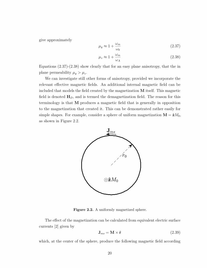
We can investigate still other forms of anisotropy, provided we incorporate therelevant effective magnetic fields. An additional internal magnetic field can beincluded that models the field created by the magnetization M itself. This magneticfield is denoted HD, and is termed the demagnetization field. The reason for thisterminology is that M produces a magnetic field that is generally in oppositionto the magnetization that created it. This can be demonstrated rather easily forsimple shapes. For example, consider a sphere of uniform magnetization M = zM0,as shown in Figure 2.2.

Figure 2.2. A uniformly magnetized sphere.

The effect of the magnetization can be calculated from equivalent electric surfacecurrents [2] given by

Jms = M× r (2.39)

which, at the center of the sphere, produce the following magnetic field according

20

to the Biot-Savart law.B = µ0

4π

‹

S

Jms × (−r)r2

0dS (2.40)

Note we do not compute H, since we are not dealing with free currents. Evaluatingthis integral yields

B = z2µ0M0

3 = 23µ0M (2.41)

ThenH = 1

µ0B−M = −1

3M (2.42)

It can be deduced from the solutions of Laplace’s equation that the field inside thesphere must be uniform, and hence equal to the value at its center. For simpleshapes (any ellipsoid [25]) where the induced field is uniform within the magnetizedbody, we can relate the demagnetization field H to the magnetization that causesit using a diagonal tensor N such that

H = −N ·M (2.43)

For the simple case of the sphere, we have

N = 13I (2.44)

Another example, which can be used to model thin film structures and ferromagneticlaminates, is that of an infinite slab. Consider the slab with uniform magnetizationdirected normal to its two interfaces, as shown in Figure 2.3.

Figure 2.3. A uniformly magnetized infinite slab.

In this case Jms = M × ±z = 0. We immediately conclude that B = 0everywhere. Hence, in the slab, H = 1

µ0B −M = −M. If, instead, we had

magnetization M = xM0 or yM0, then along the top and bottom interfaces thecurrents are oppositely directed. From this, it is clear that B = 0 outside the slab,and hence H = 1

µ0B = 0 outside the slab as well. Then from the requirement that

21

the tangential H fields be continuous across the interface (note that there are nofree currents), it follows that H = 0 within the slab. We obtain for the infinite slabthe demagnetization tensor

N = zz (2.45)

Thus in the case of both the sphere and the slab, the demagnetization field is alwaysuniform and oppositely directed to the magnetization that created it. This doesnot mean that the total magnetization is antiparallel to the total demagnetizationfield. In the case of the slab, for example, we could set M = xMx + zMz, andobtain a demagnetization field H = −zMz, which is not antiparallel to M.

The demagnetization field can be readily incorporated into the equation ofmotion for the magnetization within a domain. In (2.12), we now set

H = HA + HRF + HD (2.46)

We consider two thin film configurations.Suppose that we have a thin magnetic domain with static magnetization and

anisotropy field pointing out of the plane. That is, we set MS = zMS, N = zz,and HA = zHA. First, we compute the newly incorporated term involving thedemagnetization field.

M×HD = (zMS + MRF )× (−N) · (zMS + MRF ) (2.47)

This reduces to

M×HD = −MRF × zMS −MRF × zMRFz (2.48)

Assuming the external oscillating fields are much smaller in magnitude than theinternal fields, we may neglect the second nonlinear term. Hence,

M×HD = −MRF × zMS (2.49)

Combining (2.12), (2.46), and (2.49), we obtain the equation of motion for a thinfilm with magnetization directed out of the plane.

jωMRF = −ωmz×HRF + (ω0 − ωm)z×MRF (2.50)

22

Solving this equation yields the permeability tensor

µ = µf (I− zz)− jκf z× I + zz (2.51)

whereµf = 1 + ωm(ω0 − ωm)

(ω0 − ωm)2 − ω2 (2.52)

κf = ωωm(ω0 − ωm)2 − ω2 (2.53)

Equations (2.52) and (2.53), when compared to (2.25) and (2.26), show that thepresence of the demagnetization field has altered the formulas for the permeabilitytensor elements. Often, for ferromagnetic thin films, it is the case that MS � HA,and hence ωM � ω0 [32]. Furthermore, if we limit ourselves to frequencies below1 GHz, then it is also true that ωm � ω. In this case, (2.52) shows that µf ≈ 0.Similarly, from (2.53), we have κf ≈ 0. Thus, for many ferromagnetic films, ifthe static magnetization is directed out of the plane, the permeability tensor isapproximately [32]

µ ≈ zz (2.54)

Equation (2.54) indicates that the permeability associated with static magnetizationpointed out of the film plane is negligible.

For the case of an in plane static magnetization and anisotropy field, we setMS = xMS, N = zz, and HA = xHA. The resulting equation governing themagnetization is

jωMRF = −ωmx×HRF + ω0x×MRF − ωmyMRFz (2.55)

whose solution gives

µ = xxµx + yyµy + zzµz − jκf x× I (2.56)

whereµx = 1 (2.57)

µy = 1 + ωm(ω0 + ωm)ω0(ω0 + ωm)− ω2 (2.58)

23

µz = 1 + ωmω0

ω0(ω0 + ωm)− ω2 (2.59)

κf = ωωmω0(ω0 + ωm)− ω2 (2.60)

These results are somewhat similar to the case of an easy plane anisotropy field, asgiven in (2.32)-(2.36). Under the (often satisfied) approximation ωm � ω0 � ω,the limiting behavior of (2.57)-(2.60) gives [32]

µy ≈ 1 + ωmω0

(2.61)

µz ≈ 2 (2.62)

κf ≈ 0 (2.63)

In this case, the thin film exhibits significant permeability along the in-plane axisthat is perpendicular to the axis of static magnetization. Thus, y is the hard axisof the domain, and x is the easy axis.

2.2 Crystal-Oriented FerritesFerrites are crystalline oxides of ferromagnetic elements [25]. For a crystalline

ferrite, the prediction of its dynamic permeability will depend on a number ofparameters that are, in reality, intrinsic to its chemical composition and themanufacturing process used for its synthesis. It is beyond the scope of this sectionto delve into the details of material chemistry or synthesis. Instead, we will putforth some assumptions regarding the arrangement of magnetic domains, and thenattempt to estimate the resulting permeability.

The possibility of obtaining macroscopically anisotropic magnetic materialsexists because of the inherent anisotropy of single crystals. In a single crystal,the inherent crystalline anisotropy fields are shared across its magnetic domains.Thus, while no net magnetization exists within a demagnetized crystal, therecould be some special ordering of the internal magnetization. For example, auniaxial grain is likely to possess domains with easy axes lying along a sharedcrystal axis. For this grain, we obtain the picture of many domains, with eitheran “up” or “down” orientation, according to the ± orientation of the domainmagnetization with respect to the crystal axis [28]. In a polycrystalline ferrite,

24

there would exist many small crystal grains [28]. For most polycrystalline ferrites,there is no special ordering of the easy axes of the grains, and the overall samplepossesses a macroscopically isotropic permeability [28]. However, it is possible tomanipulate the orientation of the grains during the manufacturing process. Thiscan be accomplished by application of a slowly rotating RF magnetic field duringthe sintering process [33] [34]. Ferrite materials that have been produced in thisway are commonly described as “crystal-oriented”, or “textured”. Crystal-orientedferrite materials with macroscopically anisotropic permeability, even in the initiallydemagnetized state, have been reported [33], [34].

We will consider the anisotropy of a single uniaxial crystal, comprising domainsaligned with a shared easy axis, which we take to be z. We suppose that thedomains’ magnetization vectors are oriented along either +z or −z. The effectiveanisotropy field in each domain, HA, is parallel to its magnetization. Moreover, weshall assume that the crystal is in the form of a long thin rod, with the easy axesdirected along its long dimension. The demagnetization fields for this geometrywill be small and are thus ignored. Accordingly, the permeability tensors for ±domains are obtained from (2.24)-(2.26), and (2.29) as

µ± = µd(I− nn)∓ jκdn× I + nn (2.64)

whereµd = 1 + (ω0 + jωα)ωm

(ω0 + jωα)2 − ω2 (2.65)

κd = ωωm(ω0 + jωα)2 − ω2 (2.66)

The main challenge in accounting for dynamic domain interactions is that preciseinformation on domain size and shape distributions are unknown. Thus, thetheoretical approach needs to account for interactions in an approximate waythat is, in some sense, independent of this missing information. A perturbationalformulation of the Bruggeman-type effective medium theory was suggested byBouchaud and Zerah [35]. They provided no derivational details, so on account ofthe theory’s fundamental importance, we give a proof of their results.

The first step in the derivation is to make a hypothesis regarding the generalform of the effective medium model. We propose that the single crystal comprisingup and down domains can be modeled as an effective medium with a permeability

25

tensor of the formµg = µg(I− nn)− jκgn× I + nn (2.67)

This hypothesis is reasonable, since this template for the permeability tensormatches that of both domain types. We do not expect that µg or κg should beequal to µd and κd.

If each domain within the crystal is not overly large compared to the crystalitself, then each domain must experience the environment of being within thecrystal, as if it was submerged in a larger body with the effective medium propertiesassumed by (2.67). We make two separate calculations. First, we submerge asmall cylindrically shaped + domain into a larger body with permeability describedby (2.67), and calculate the new permeability that arises as a consequence of thepresence of the small inclusion. Let this new permeability be

µ+ δµ+ (2.68)

Second, we repeat this calculation with a small − domain immersed in the effectivemedium, and calculate the new permeability as

µ+ δµ− (2.69)

Further, we suppose that the relative fractions of +, and − domains appearingwithin the grain are 1+m

2 , and 1−m2 , respectively, where 0 < m < 1

2 . The proposedeffective medium model is internally logically consistent, provided the sum of thetwo perturbations, weighted by their relative fractions, is zero. We require

1 +m

2 δµ+ + 1−m2 δµ− = 0 (2.70)

We assume the tensor perturbations have the same form as µ, except with parametersδµ± and δκ±. Thus (2.70), by taking sums and differences of δµ± and δκ± isequivalent to requiring

1 +m

2 (δµ+ ± δκ+) + 1−m2 (δµ− ± δκ−) = 0 (2.71)

The method for calculating the perturbations is to determine the average B and Hfields for an assumed external field of polarization u = x± jy. Then, according to

26

(2.27), forming the ratio of the average fields BH

will yield µeff ± κeff . Then, sinceµeff = µg + δµ± and κeff = κg + δκ±, we will obtain from (2.71), 2 equations inthe 2 unknowns µg and κg.

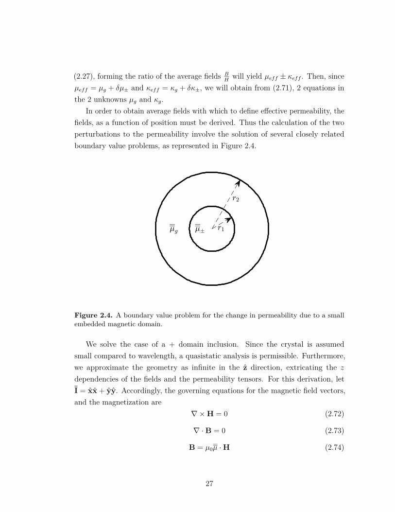
In order to obtain average fields with which to define effective permeability, thefields, as a function of position must be derived. Thus the calculation of the twoperturbations to the permeability involve the solution of several closely relatedboundary value problems, as represented in Figure 2.4.

Figure 2.4. A boundary value problem for the change in permeability due to a smallembedded magnetic domain.

We solve the case of a + domain inclusion. Since the crystal is assumedsmall compared to wavelength, a quasistatic analysis is permissible. Furthermore,we approximate the geometry as infinite in the z direction, extricating the zdependencies of the fields and the permeability tensors. For this derivation, letI = xx + yy. Accordingly, the governing equations for the magnetic field vectors,and the magnetization are

∇×H = 0 (2.72)

∇ ·B = 0 (2.73)

B = µ0µ ·H (2.74)

27

From (2.72), we can set H = ∇ψ. Hence, (2.72)-(2.74) may be combined obtaining

∇ ·B = 0

∇ · (µ± · (∇ψ)) = 0

∇ · ((Iµd ∓ jκdz× I) · ∇ψ) = 0

µd∇ · ∇ψ ∓ jκd∇ · (z×∇ψ) = 0

µd∇2ψ ± jκd∇ · (∇× (zψ)) = 0

∇2ψ = 0 (2.75)

The solutions to (2.75) in cylindrical coordinates, with no z variation, are [2]

ψm = ρme±jmφ (2.76)

andψm = ρ−me±jmφ (2.77)

Now we observe for m = 1, that we may obtain

H = ∇ψ1 = H0∇ρejφ = H0∇(x+ jy) = H0(x + jy) (2.78)

Fields of this form will experience an isotropic permeability µd + κd within thedomain, and µg + κg in the effective medium layer surrounding the domain. Wenumber the regions 1, 2, 3 for the domain, effective medium, and free space, re-spectively. We require that the field in region 3 goes to a uniform external fieldH = H0(x + jy) at large distances. Singular ρ−1 solutions are excluded from region1. Appropriate general solutions are

ψ1 = A1ρejφ

ψ2 = (A2ρ+B2ρ−1)ejφ

ψ3 = (H0ρ+B3ρ−1)ejφ

(2.79)

The associated B and H fields computed from (2.72) and (2.74) are

H1 = A1(ρ+ jφ)ejφ

H2 = ρ(A2 −B2ρ−2)ejφ + φj(A2 +B2ρ

−2)ejφ

28

H3 = ρ(H0 −B3ρ−2)ejφ + φj(H0 +B3ρ

−2)ejφ

B1 = A1µ0(µd + κd)(ρ+ jφ)ejφ (2.80)

B2 = ρµ0((µg + κg)A2 − (µg − κg)B2ρ−2)ejφ

+ φjµ0((µg + κg)A2 + (µg − κg)B2ρ−2)ejφ

B3 = ρµ0(H0 −B3ρ−2)ejφ + φjµ0(H0 +B3ρ

−2)ejφ

The H and B fields must satisfy the boundary conditions

φ · (H1 −H2)|ρ=r1 = 0

φ · (H2 −H3)|ρ=r2 = 0

ρ · (B1 −B2)|ρ=r1 = 0

ρ · (B2 −B3)|ρ=r2 = 0

(2.81)

Substitution of the field expressions into the boundary conditions leads to a systemof linear equations in the unknown coefficients. Solving these equations for thecoefficients A1 and A2, we obtain

A1 = 4µgr−22 H0∆−1

A2 = 2((µd + κd) + (µg − κg))r−22 H0∆−1

(2.82)

where

∆ = (µg − κg − 1)((µd + κd)− (µg + κg))− (1 + µg + κg)((µd + κd) + (µg − κg))

The values of the coefficients B1 and B2 are unimportant, as we will now show bycomputing the field averages. For example, working with H1, we first convert thefield expression back to Cartesian coordinates

H1 = A1(x + jy)

Then the field average over region 1 is

H1avg = 1πr2

1

r1ˆ

0

2πˆ

0

A1(x + jy)ρdφdρ

29

H1avg = A1(x + jy)

Similarly,

H2avg = A2(x + jy)

B1avg = A1µ0(µd + κd)(x + jy)

B2avg = A2µ0(µg + κg)(x + jy)

Averages over the entire grain then yield

Havg = (x + jy)r21A1 + (r2

2 − r21)A2

(r1 + r2)2

Bavg = (x + jy)r21(µd + κd)A1 + (r2

2 − r21)(µg + κg)A2

(r1 + r2)2

Taking the ratio of the average fields, we obtain

(µg + δµ+) + (κg + δκ+) = r21(µd + κd)A1 + (r2

2 − r21)(µg + κg)A2

r21A1 + (r2

2 − r21)A2

(2.83)

Substitution of (2.82) into (2.83), and solving for δµ+ + δκ+ yields

δµ+ + δκ+ = 2r21µg((µd + κd)− (µg + κg))

2r21µg + (r2

2 − r21)((µd + κd) + (µg − κg))

(2.84)

Next, we assume r22 � r2

1, and argue that the term 2r21µg in the denominator may

be ignored. If we define a surface filling fraction ϕ = r21(r2

2 − r21)−1, then (2.84)

becomesδµ+ + δκ+ = 2µgϕ

(µd + κd)− (µg + κg)(µd + κd) + (µg − κg)

(2.85)

This process can be repeated with an external field x − jy to determine δµ+ −δκ+. Then both calculations would be repeated with a − domain instead of a+ domain. Actually, though, the required results can be obtained immediatelywithout reworking the boundary value problem. For example, for the case of a +domain and an external field with opposite rotation sense x + jy, we can replaceκd with −κd, and κg with −κg, obtaining

δµ+ − δκ+ = 2µgϕ(µd − κd)− (µg − κg)(µd − κd) + (µg + κg)

(2.86)

30

Similarly, by further replacing κd with −κd in (2.85) and (2.86), we obtain, respec-tively

δµ− + δκ− = 2µgϕ(µd − κd)− (µg + κg)(µd − κd) + (µg − κg)

(2.87)

δµ− − δκ− = 2µgϕ(µd + κd)− (µg − κg)(µd + κd) + (µg + κg)

(2.88)

Substitution of (2.85)-(2.88) into (2.71) leads to two equations in the unknowns µgand κg.(

1 +m

2

)(µd + κd)− (µg + κg)(µd + κd) + (µg − κg)

+(

1−m2

)(µd − κd)− (µg + κg)(µd − κd) + (µg − κg)

= 0 (2.89)

(1 +m

2

)(µd − κd)− (µg − κg)(µd − κd) + (µg + κg)

+(

1−m2

)(µd + κd)− (µg − κg)(µd + κd) + (µg + κg)

= 0 (2.90)

From (2.89) and (2.90), it can be shown that

µ2g − κ2

g = µ2d − κ2

d (2.91)

κg = mκdµgµd

(2.92)

Equations (2.91) and (2.92) define the effective properties of the uniaxial crystalin terms of the properties of its magnetic domains. In the initially demagnetizedstate, we assume that m = 0, hence

µg =√µ2d − κ2

d (2.93)

and κg = 0. The permeability tensor for the uniaxial crystal is thus

µg = (xx + yy)√µ2d − κ2

d + zz (2.94)

For a polycrystalline ferrite with isotropically distributed uniaxial crystal grains,we assume the isotropic permeability is given by the average of the permeabilityalong the three directions given in (2.94), obtaining

µeff = 13 + 2

3

√µ2d − κ2

d (2.95)

This is the result first discovered by Schlomann for a specific domain arrangement

31

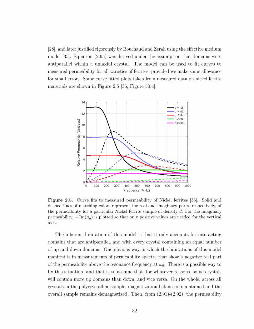
[28], and later justified rigorously by Bouchaud and Zerah using the effective mediummodel [35]. Equation (2.95) was derived under the assumption that domains wereantiparallel within a uniaxial crystal. The model can be used to fit curves tomeasured permeability for all varieties of ferrites, provided we make some allowancefor small errors. Some curve fitted plots taken from measured data on nickel ferritematerials are shown in Figure 2.5 [36, Figure 50.4].

0 100 200 300 400 500 600 700 800 900 1000

Frequency (MHz)

0

2

4

6

8

10

12

14

Rel

ativ

e P

erm

eabi

lity

(Uni

tless

)

d=4.18d=4.02d=3.44d=3.32d=3.06

Figure 2.5. Curve fits to measured permeability of Nickel ferrites [36]. Solid anddashed lines of matching colors represent the real and imaginary parts, respectively, ofthe permeability for a particular Nickel ferrite sample of density d. For the imaginarypermeability, − Im(µg) is plotted so that only positive values are needed for the verticalaxis.

The inherent limitation of this model is that it only accounts for interactingdomains that are antiparallel, and with every crystal containing an equal numberof up and down domains. One obvious way in which the limitations of this modelmanifest is in measurements of permeability spectra that show a negative real partof the permeability above the resonance frequency at ω0. There is a possible way tofix this situation, and that is to assume that, for whatever reasons, some crystalswill contain more up domains than down, and vice versa. On the whole, across allcrystals in the polycrystalline sample, magnetization balance is maintained and theoverall sample remains demagnetized. Then, from (2.91)-(2.92), the permeability

32

of each grain is

µg =√√√√ µ2

d − κ2d

1− (mκd

µd)2 (2.96)

Permeability spectra computed with (2.96) can achieve values with negative realpart 3. We are primarily interested, however, in the properties of magnetic materialsbelow resonance, and in this regime, (2.95) works well enough.

Useful insights can be gained from (2.95). For example, by examining thepermeability at zero frequency and at resonance a very useful relationship can beobtained. Setting ω = 0 in (2.95), one obtains for the DC permeability the simpleformula

µDC = 1 + 23ωmω0

(2.97)

A resonance occurs at ωres = ω0. (Referring to Figure 2.5, for lossy materials,the resonance frequency ω0 can be determined from plots by taking the frequencywhere the imaginary component of the permeability is a maximum.) From (2.97),multiplying by ω0 on both sides yields

ωres(µDC − 1) = 23ωm (2.98)

This famous relationship is known widely as Snoek’s law [37, Equation 3c]. Itstates that for a particular internal magnetization, that the product of the DCpermeability and resonance frequency is a fixed constant. Stated differently, theDC permeability and resonance frequency, for a class of materials sharing the samemagnetization, will be inversely related. That is, if one material, possessing a givenmagnetization equal to another material, has a comparatively higher resonancefrequency, then it must have a comparatively lower DC permeability, and viceversa.

Alternatively, we could have obtained Snoek’s law directly from the propertiesof the magnetic domains. The DC permeability along the hard axes of a domain

3If using ejωt time convention and attempting to compute (2.96), the branch cut of the squareroot function must be placed along the positive real axis in the complex plane. This is not theprincipal value of the square root adopted by modern scientific computing packages. To get thecorrect result, use the definition √

z = −√|z| ejθ/2

with θ the phase angle of z taken from the range (0, 2π].

33

with a uniaxial anisotropy field can be obtained from (2.65) as

µd|ω=0 = 1 + ωmω0

(2.99)

Then, at zero frequency there is no dynamic interaction between domains. Thusthe overall DC permeability can be estimated from (2.99). The permeability alongthe two hard axes is given by (2.99), while along the easy axis it is equal to 1. Thusthe average of these permeabilities yields 1 + 2

3ωm

ω0. Furthermore, the resonance

frequency for the domain, from (2.65), is still ω0. Combining these results we obtainSnoek’s law.

This simpler approach enables us to quickly obtain the analogous “Snoek’s Law”for a ferrite possessing an easy plane for magnetization. Referring to (2.33)-(2.35),the DC permeabilities for a domain with an easy plane anisotropy are

µx = 1

µy = 1 + ωmω0

µz = 1 + ωmω0 + ωA

The average of these three directional permeabilities gives

µDC = 1 + ωm3

(1ω0

+ 1ω0 + ωA

)(2.100)

The resonance frequency is obtained by setting the denominator of either (2.34) or(2.35) equal to zero and solving for ω, obtaining

ωres =√ω0(ω0 + ωA) (2.101)

Combining (2.100) and (2.101), we obtain [36, Equation 51.2]

ωres(µDC − 1) = ωm3

√ω0 + ωAω0

+√

ω0

ω0 + ωA

(2.102)

34

Since ωA � ω0 [36, See Table 51.1], we have approximately

ωres(µDC − 1) = ωm3

√ωAω0

(2.103)

Since ωA � ω0, the right hand side of (2.103) can be much larger than in (2.98).In practice, this means that easy plane ferrites can possess larger permeabilitiesat higher frequencies than uniaxial ferrites. This can be seen by comparing theextracted permeability spectra for some measured easy plane ferrites [38] shown inFigure 2.6, to the nickel ferrites of Figure 2.5.

0 200 400 600 800 1000 1200 1400 1600 1800 2000

Frequency (MHz)

0

5

10

15

Rel

ativ

e P

erm

eabi

lity

(Uni

tless

)

X=0.5X=0.4X=0.3X=0.2X=0

Figure 2.6. Curve fits to measured permeability of Barium ferrites with easy planeanisotropy. Solid and dashed lines of a particular color give the real and imaginary partsof the permeability, respectively, for a Barium ferrite with X percent Zinc doping.

The permeability of easy plane ferrites can be further increased by applying aplanar rotating magnetic field to the ferrite during production. This field will exerta torque force on the crystals, because of the strong out of plane anisotropy field Hθ.Provided the ferrite has not yet crystallized, and is rather still in a slurry-like phase,then the individual particles are free to rotate under the action of the externalmagnetic field. The applied force is such that the easy plane aligns with the planeof applied magnetic field. Crystal-oriented easy plane ferrites were first reported byStuijts and Wijn [33].

35

Unfortunately, no direct formulations, like the perturbational Bruggeman modelfor interacting domains in uniaxial crystals, have been given for the directionalpermeability spectra of crystal oriented easy plane ferrites. We can make someinferences without a detailed model, based on the study of a uniaxial ferrite and theformulations of Snoek’s laws. For the uniaxial ferrite, the macroscopic permeabilitywas isotropic only because an isotropic distribution of crystal orientations wasassumed. If there was, on average, a preferential alignment of these single crystalswithin the overall sample, then a macroscopically anisotropic permeability wouldbe expected. Assuming appropriate axes are chosen, this permeability can beexpressed by a diagonal tensor

µ = xxµx + yyµy + zzµz (2.104)

For an easy plane ferrite with crystals oriented using an in-plane rotating magneticfield, we expect the permeabilities µx and µy to be larger than µz. Assumingall of the magnetization lies in plane, then the expected increase of the in planepermeability would be a factor of about 3/2. That is, the DC permeability alongany direction within the plane is expected to be given by the average of µx and µygiven in (2.33)-(2.34)

µDCt = 1 + 12ωmω0

(2.105)

Similarly, the out of plane DC permeability would be given by (2.35) as approxi-mately

µDCn = 1 + ωmωA

(2.106)

In this estimate, we have implicitly assumed that the in-plane anisotropy fieldwould not be affected by the in plane crystal alignment. Measurement comparisonsof both oriented and non-oriented samples of the same ferrite species show that theincrease of the in plane permeability is actually more pronounced [36]. Furthermore,the resonance frequency of the oriented sample is decreased compared to thenon-oriented sample [36]. These two facts, taken together, suggest that the inplane anisotropy field is weakened within the crystal oriented sample. Additionally,the easy-plane crystals are probably not completely aligned. The out of planepermeability is thus expected to be higher than that predicted by (2.106). In

36

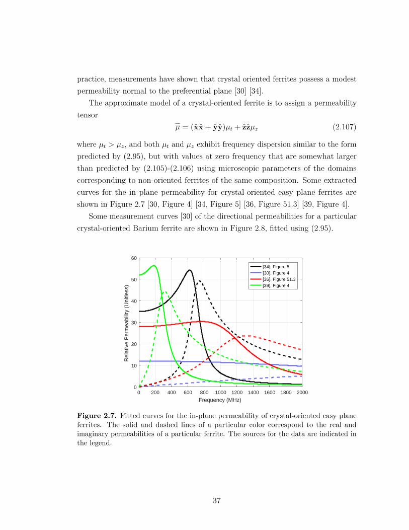
practice, measurements have shown that crystal oriented ferrites possess a modestpermeability normal to the preferential plane [30] [34].

The approximate model of a crystal-oriented ferrite is to assign a permeabilitytensor

µ = (xx + yy)µt + zzµz (2.107)

where µt > µz, and both µt and µz exhibit frequency dispersion similar to the formpredicted by (2.95), but with values at zero frequency that are somewhat largerthan predicted by (2.105)-(2.106) using microscopic parameters of the domainscorresponding to non-oriented ferrites of the same composition. Some extractedcurves for the in plane permeability for crystal-oriented easy plane ferrites areshown in Figure 2.7 [30, Figure 4] [34, Figure 5] [36, Figure 51.3] [39, Figure 4].

Some measurement curves [30] of the directional permeabilities for a particularcrystal-oriented Barium ferrite are shown in Figure 2.8, fitted using (2.95).

0 200 400 600 800 1000 1200 1400 1600 1800 2000

Frequency (MHz)

0

10

20

30

40

50

60

Rel

ativ

e P

erm

eabi

lity

(Uni

tless

)

[34], Figure 5[30], Figure 4[36], Figure 51.3[39], Figure 4

Figure 2.7. Fitted curves for the in-plane permeability of crystal-oriented easy planeferrites. The solid and dashed lines of a particular color correspond to the real andimaginary permeabilities of a particular ferrite. The sources for the data are indicated inthe legend.

37

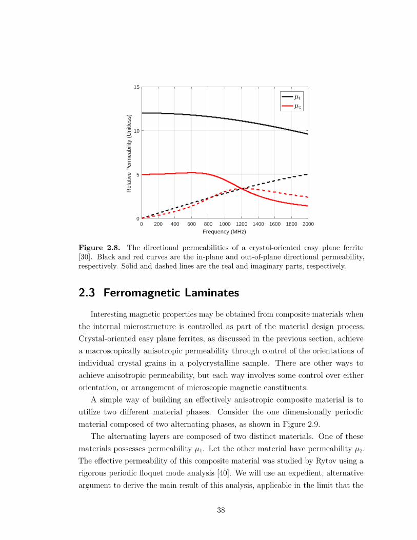
0 200 400 600 800 1000 1200 1400 1600 1800 2000

Frequency (MHz)

0

5

10

15

Rel

ativ

e P

erm

eabi

lity

(Uni

tless

)

Figure 2.8. The directional permeabilities of a crystal-oriented easy plane ferrite[30]. Black and red curves are the in-plane and out-of-plane directional permeability,respectively. Solid and dashed lines are the real and imaginary parts, respectively.

2.3 Ferromagnetic LaminatesInteresting magnetic properties may be obtained from composite materials when

the internal microstructure is controlled as part of the material design process.Crystal-oriented easy plane ferrites, as discussed in the previous section, achievea macroscopically anisotropic permeability through control of the orientations ofindividual crystal grains in a polycrystalline sample. There are other ways toachieve anisotropic permeability, but each way involves some control over eitherorientation, or arrangement of microscopic magnetic constituents.

A simple way of building an effectively anisotropic composite material is toutilize two different material phases. Consider the one dimensionally periodicmaterial composed of two alternating phases, as shown in Figure 2.9.

The alternating layers are composed of two distinct materials. One of thesematerials possesses permeability µ1. Let the other material have permeability µ2.The effective permeability of this composite material was studied by Rytov using arigorous periodic floquet mode analysis [40]. We will use an expedient, alternativeargument to derive the main result of this analysis, applicable in the limit that the

38

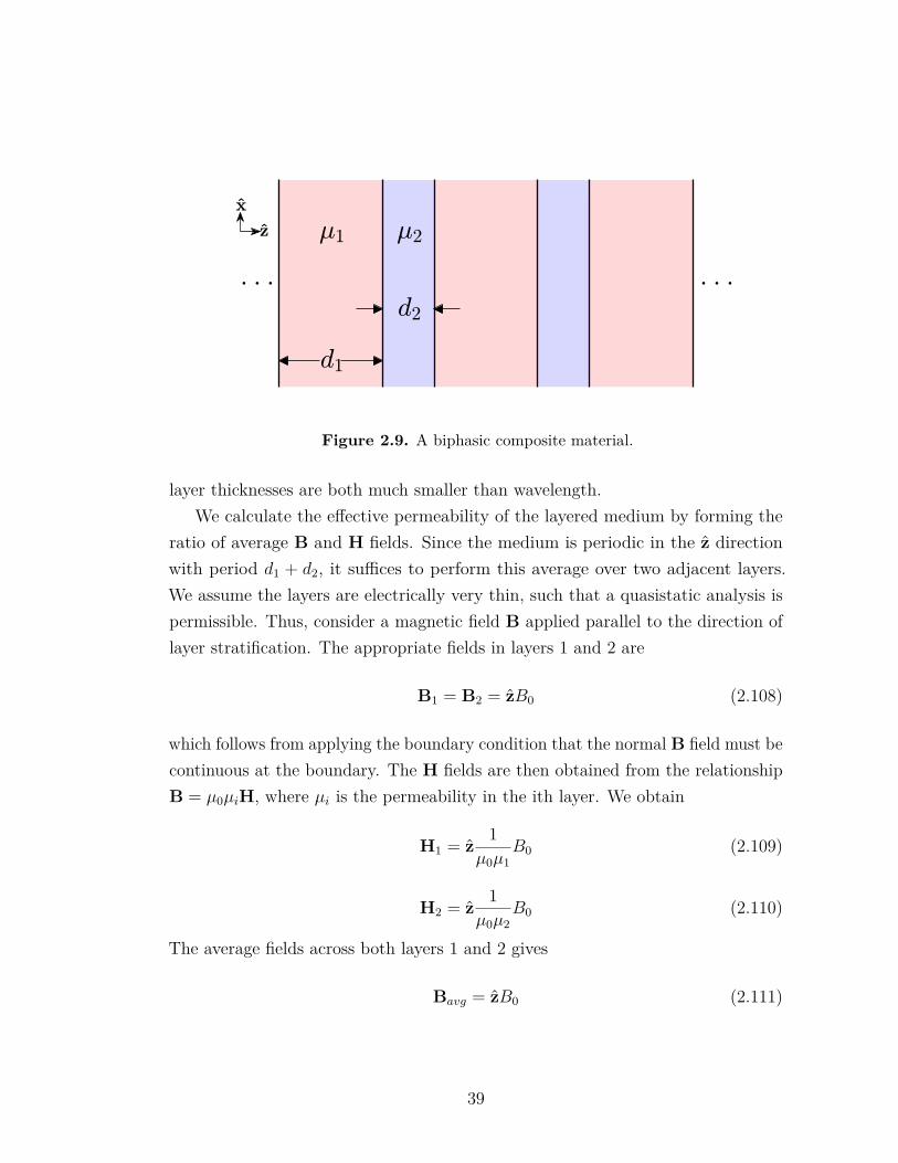
Figure 2.9. A biphasic composite material.

layer thicknesses are both much smaller than wavelength.We calculate the effective permeability of the layered medium by forming the

ratio of average B and H fields. Since the medium is periodic in the z directionwith period d1 + d2, it suffices to perform this average over two adjacent layers.We assume the layers are electrically very thin, such that a quasistatic analysis ispermissible. Thus, consider a magnetic field B applied parallel to the direction oflayer stratification. The appropriate fields in layers 1 and 2 are

B1 = B2 = zB0 (2.108)

which follows from applying the boundary condition that the normal B field must becontinuous at the boundary. The H fields are then obtained from the relationshipB = µ0µiH, where µi is the permeability in the ith layer. We obtain

H1 = z1

µ0µ1B0 (2.109)

H2 = z1

µ0µ2B0 (2.110)

The average fields across both layers 1 and 2 gives

Bavg = zB0 (2.111)

39

Havg = zB0

µ0

µ2d1 + µ1d2

µ1µ2(d1 + d2) (2.112)

Taking the ratio of (2.111) and (2.112) we obtain the z directional permeability

µz = µ1µ2(d1 + d2)µ2d1 + µ1d2

(2.113)

For fields parallel to the interface, assume that the H fields are

H1 = H2 = xH0 (2.114)

Then the B fields areB1 = xµ0µ1H0 (2.115)

B2 = xµ0µ2H0 (2.116)

and the average fields becomeHavg = xH0 (2.117)

Bavg = xµ0H0d1µ1 + d2µ2

d1 + d2(2.118)

Forming the ratio of (2.118) and (2.117), we find the permeability transverse tothe layer stratification is

µt = d1µ1 + d2µ2

d1 + d2(2.119)

Thus the composite material is anisotropic, with directional permeabilities µz andµt. The permeability tensor is evidently µ = (xx + yy)µt + zzµz.

A natural motivation for building a composite material of this variety is to takeadvantage of magnetic properties inherent in a thin film geometry. The behaviorof magnetic domains in a very thin film was discussed in Section 2.1.2. Since thepermeability associated with magnetization tilted out of the film plane is negligible,and also since the demagnetization fields tend to make such a configuration unstable,it is reasonable to assume that the static magnetization of the domains lies inthe film plane. Depending on the preparation of the film, the entire film couldconsist of a single magnetic domain, or many domains with distributed orientationswithin the film plane [41]. If the film is a single magnetic domain, then it isalso uniformly magnetized by definition, and its permeability below resonancealong the hard axis is approximately given by (2.61). The resonance frequency

40

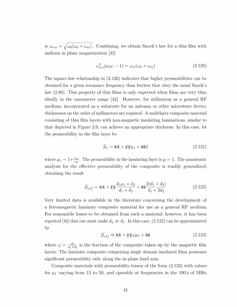
is ωres =√ω0(ω0 + ωm) . Combining, we obtain Snoek’s law for a thin film with

uniform in plane magnetization [42]

ω2res(µDC − 1) = ωm(ω0 + ωm) (2.120)

The square-law relationship in (2.120) indicates that higher permeabilities can beobtained for a given resonance frequency than ferrites that obey the usual Snoek’slaw (2.98). This property of thin films is only expected when films are very thin,ideally in the nanometer range [42]. However, for utilization as a general RFmedium, incorporated as a substrate for an antenna or other microwave device,thicknesses on the order of millimeters are required. A multilayer composite materialconsisting of thin film layers with non-magnetic insulating laminations, similar tothat depicted in Figure 2.9, can achieve an appropriate thickness. In this case, letthe permeability in the film layer be

µ1 = xx + yyµ1 + zz2 (2.121)

where µ1 = 1+ωm

ω0. The permeability in the insulating layer is µ = 1. The quasistatic

analysis for the effective permeability of the composite is readily generalized,obtaining the result

µeff = xx + yyd1µ1 + d2

d1 + d2+ zz

2(d1 + d2)d1 + 2d2

(2.122)

Very limited data is available in the literature concerning the development ofa ferromagnetic laminate composite material for use as a general RF medium.For reasonable losses to be obtained from such a material; however, it has beenreported [42] that one must make d2 � d1. In this case, (2.122) can be approximatedby

µeff ≈ xx + yyϕµ1 + zz (2.123)

where ϕ = d1d1+d2

is the fraction of the composite taken up by the magnetic filmlayers. The laminate composite comprising single domain insulated films possessessignificant permeability only along the in-plane hard axis.

Composite materials with permeability tensor of the form (2.123) with valuesfor µ1 varying from 15 to 50, and operable at frequencies in the 100’s of MHz,

41

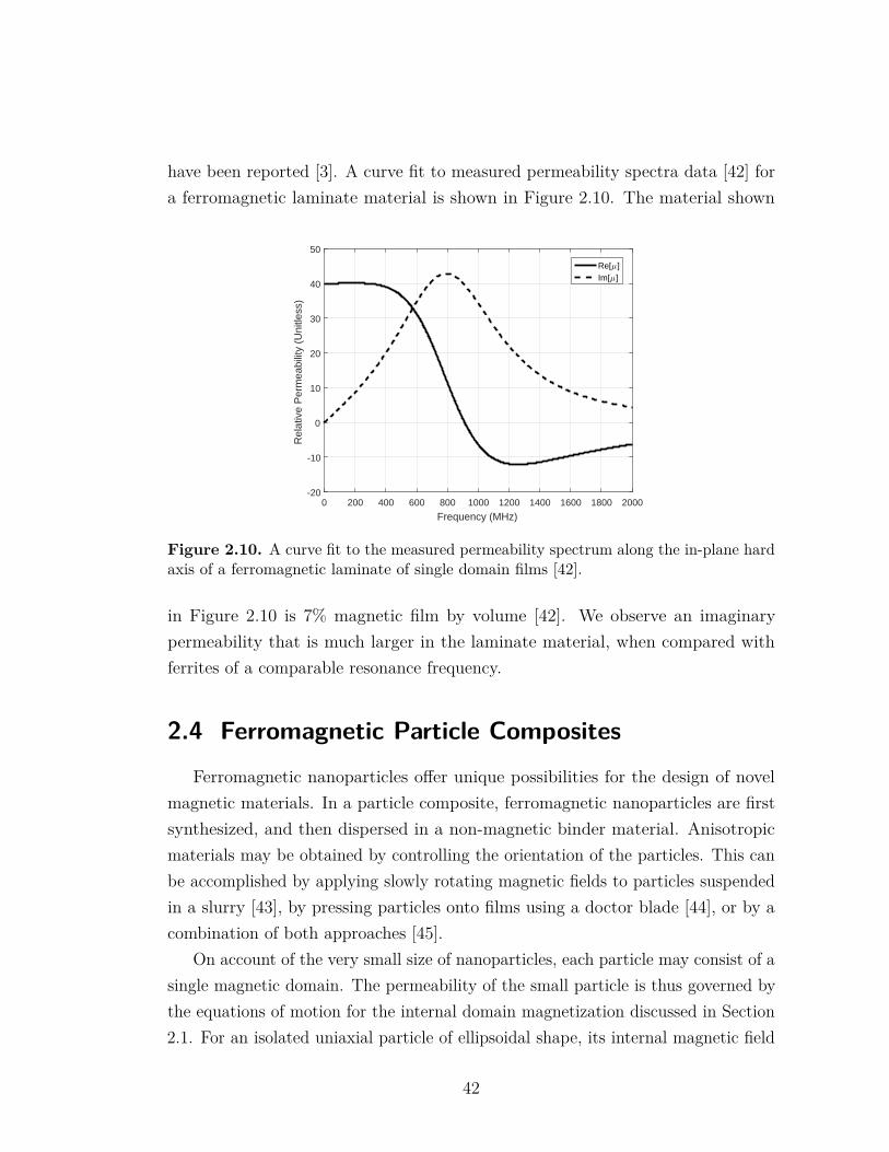
have been reported [3]. A curve fit to measured permeability spectra data [42] fora ferromagnetic laminate material is shown in Figure 2.10. The material shown

0 200 400 600 800 1000 1200 1400 1600 1800 2000

Frequency (MHz)

-20

-10

0

10

20

30

40

50

Rel

ativ

e P

erm

eabi

lity

(Uni

tless

)

Re[ ]Im[ ]

Figure 2.10. A curve fit to the measured permeability spectrum along the in-plane hardaxis of a ferromagnetic laminate of single domain films [42].

in Figure 2.10 is 7% magnetic film by volume [42]. We observe an imaginarypermeability that is much larger in the laminate material, when compared withferrites of a comparable resonance frequency.

2.4 Ferromagnetic Particle CompositesFerromagnetic nanoparticles offer unique possibilities for the design of novel

magnetic materials. In a particle composite, ferromagnetic nanoparticles are firstsynthesized, and then dispersed in a non-magnetic binder material. Anisotropicmaterials may be obtained by controlling the orientation of the particles. This canbe accomplished by applying slowly rotating magnetic fields to particles suspendedin a slurry [43], by pressing particles onto films using a doctor blade [44], or by acombination of both approaches [45].

On account of the very small size of nanoparticles, each particle may consist of asingle magnetic domain. The permeability of the small particle is thus governed bythe equations of motion for the internal domain magnetization discussed in Section2.1. For an isolated uniaxial particle of ellipsoidal shape, its internal magnetic field

42

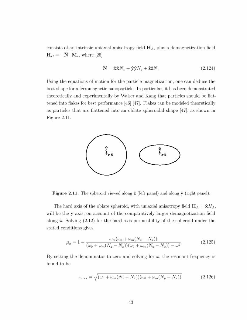
consists of an intrinsic uniaxial anisotropy field HA, plus a demagnetization fieldHD = −N ·Ms, where [25]

N = xxNx + yyNy + zzNz (2.124)

Using the equations of motion for the particle magnetization, one can deduce thebest shape for a ferromagnetic nanoparticle. In particular, it has been demonstratedtheoretically and experimentally by Walser and Kang that particles should be flat-tened into flakes for best performance [46] [47]. Flakes can be modeled theoreticallyas particles that are flattened into an oblate spheroidal shape [47], as shown inFigure 2.11.

Figure 2.11. The spheroid viewed along z (left panel) and along y (right panel).

The hard axis of the oblate spheroid, with uniaxial anisotropy field HA = xHA,will be the y axis, on account of the comparatively larger demagnetization fieldalong z. Solving (2.12) for the hard axis permeability of the spheroid under thestated conditions gives

µy = 1 + ωm(ω0 + ωm(Nz −Nx))(ω0 + ωm(Nz −Nx))(ω0 + ωm(Ny −Nx))− ω2 (2.125)

By setting the denominator to zero and solving for ω, the resonant frequency isfound to be

ωres =√

(ω0 + ωm(Nz −Nx))(ω0 + ωm(Ny −Nx)) (2.126)

43

The DC permeability, from (2.125) at zero frequency, is

µDC = 1 + ωmω0 + ωm(Ny −Nx)

(2.127)

From (2.126) and (2.127), the following Snoek’s relation may be obtained

ω2res(µDC − 1) = ωm(ω0 + ωm(Nz −Nx)) (2.128)

The right hand side is maximized when the quantity Nz −Nx is made positive andas large as possible, implying flattened particles so that Nz attains a value closeto 1, as in a thin film. In practice, nanoparticles have been successfully flattenedusing ball-milling machines, and resulting improvements in permeability have beendocumented [46].

In a sparsely populated mixture, the local applied magnetic field at the site ofindividual particles is different than the externally applied magnetic field. For aparticle that is not in isolation, the effective magnetic field that determines theparticle permeability should include a field contribution due to all other particleswithin the host matrix. The permeability of the individual particle and the overallcomposite are thus mutually dependent [48, Equation 5]. An easy way to show thatthe demagnetization field depends on the particle’s environment is to reconsiderthe simple case of a spherical particle with an inherent magnetization M = zM0,embedded in a magnetic medium with permeability µr, as opposed to free space.

By conducting separation of variables of Laplace’s equation in spherical coordi-nates with no azimuthal variation [2, pp. 188-192], one can show the appropriategeneral solution for the potentials and corresponding fields are

ψ1 = A1r cos θ

ψ2 = B2r−2 cos θ

H1 = A1(r cos θ − θ sin θ)

H2 = −B2r−3(r cos θ + θ sin θ)

B1 = µ0(H1 + M)

B2 = µ0µrH2

Enforcing the boundary conditions that the normal B fields and tangential H fields

44

be continuous at the boundary between the interior and exterior regions leads to asystem of 2 equations. Solving these equations for the unknown coefficient A1 gives

A1 = − M0

1 + 2µr

hence the demagnetization field is

HD = H1 = − 11 + 2µr

M (2.129)

Equation (2.129) shows that the demagnetization factors owing to the particleshape should decrease in a densely packed particle composite. Physically, whenthe composite is completely magnetic the demagnetization effects associated withparticle shape should mostly cancel owing to shared borders between particles.Referring to (2.128), if particle demagnetization factors are significantly reducedas the composite mixture becomes more densely populated, then correspondingreductions in resonant frequencies are expected. Thus for a larger frequency ofoperation, a lower particle concentration should be used. In [46], experimental datayielded a resonance frequency that was far lower than expected from (2.126). Thiswas attributed by the authors to a spatial resonance in the measurement fixture;however, it seems at least equally as likely that the resonance in their measurementsis indeed the ferromagnetic resonance. The lower ferromagnetic resonance frequencyis evidence that the particle demagnetization factors were not as expected on thebasis of the particle geometry, which is consistent with our discussion.

The effective permeability of the magnetic particle composite can be investigatedtheoretically using the method applied to the uniaxial ferrite crystal in Section 2.2.Assume the magnetic particle is embedded in the effective medium, and computethe small change in permeability of the medium owing to the particle. Thencalculate the change in permeability resulting from the inclusion of a non-magneticparticle. For isotropic, spherical magnetic particles, the result of this calculation isthe conventional Bruggeman effective medium satisfying [32, Equation 3]

ζµp − µeffµp + 2µeff

+ (1− ζ) 1− µeff1 + 2µeff

= 0 (2.130)

Since the effective medium permeability µeff influences the demagnetization factors

45

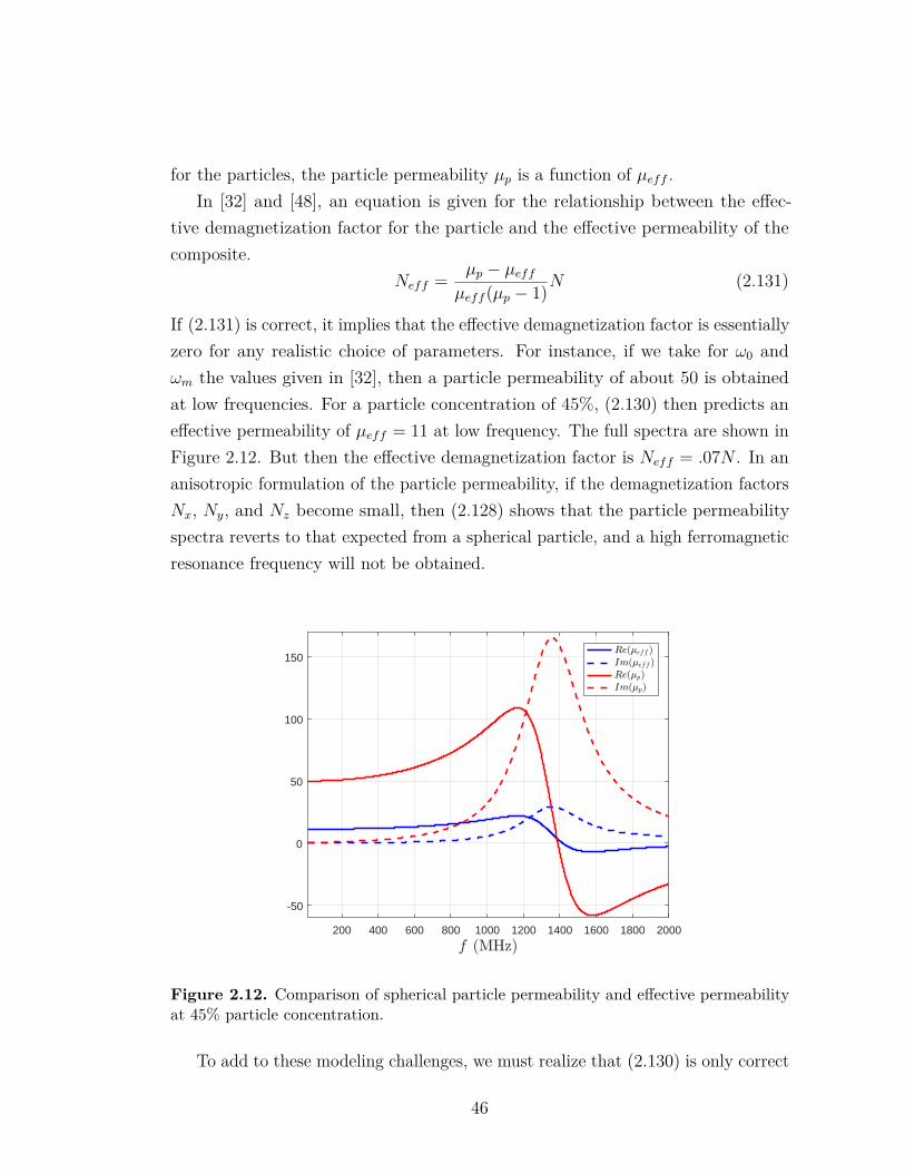
for the particles, the particle permeability µp is a function of µeff .In [32] and [48], an equation is given for the relationship between the effec-

tive demagnetization factor for the particle and the effective permeability of thecomposite.

Neff = µp − µeffµeff (µp − 1)N (2.131)

If (2.131) is correct, it implies that the effective demagnetization factor is essentiallyzero for any realistic choice of parameters. For instance, if we take for ω0 andωm the values given in [32], then a particle permeability of about 50 is obtainedat low frequencies. For a particle concentration of 45%, (2.130) then predicts aneffective permeability of µeff = 11 at low frequency. The full spectra are shown inFigure 2.12. But then the effective demagnetization factor is Neff = .07N . In ananisotropic formulation of the particle permeability, if the demagnetization factorsNx, Ny, and Nz become small, then (2.128) shows that the particle permeabilityspectra reverts to that expected from a spherical particle, and a high ferromagneticresonance frequency will not be obtained.

200 400 600 800 1000 1200 1400 1600 1800 2000

-50

0

50

100

150

Figure 2.12. Comparison of spherical particle permeability and effective permeabilityat 45% particle concentration.

To add to these modeling challenges, we must realize that (2.130) is only correct

46

for all particle concentrations provided frequencies are low. At higher frequenciesand dense particle concentrations, the particles should be close enough togetherfor the magnetic domains of the respective particles to interact with each other,in a similar fashion to that predicted by the effective medium model given forthe uniaxial crystal. One would need to include the off-diagonal components ofthe particle’s full anisotropic permeability matrix in the effective medium model.Moreover, the intrinsic dependence of the particle’s demagnetization factors onthe resultant effective medium properties would have to be ascertained. Thesecomplexities present a formidable modeling challenge. This is especially true, sinceas the number of variable parameters in a model increases, the significance of a fitto empirical data by selecting these parameters becomes increasingly doubtful.

As a consequence of these many factors involved in modeling the ferromagneticparticle composite, we shall not attempt to give a single model and pretend that itwill apply to all cases. We can, however, review some of the reported measureddata on these materials. In [45], data is given for both oriented and non-orientedZn-Ni-Fe flattened flake particles. In the sample with particles having randomorientation, µr ≈ 5, and fres ≈ 3 GHz. After particle orientation, µr increasedto 9, and the resonance frequency reduced to about 2 GHz. Walser and Kanggive measured data on two particle composites [46]. The first consists of sphericalparticles, and the second of flattened flake particles. For the spherical particles,the effective permeability of the composite is µr = 5.7. For flattened particles, thepermeability rises to µr = 42, which is a significant increase. Unfortunately, thedata does not enable a clear comparison of the ferromagnetic resonance frequenciesof the two material samples.

In both [45] and [46], the permeability is measured along an in-plane direction.Assuming flattened particles lie in the plane, the permeability should be close to 1in the normal direction. For the oriented Zn-Ni-Fe particles, mechanical pressureapplied during the deposition of flaked particles results in an additional alignmentof magnetic easy axes along a particular in-plane axis [45]. In this case, the in-planehard axis (perpendicular to the in-plane easy axis) should be the direction alongwhich the largest permeability is observed. Empirical data is not given that can beused to confirm this hypothesis.

47

Chapter 3 |Electromagnetic WavePropagation in AnisotropicMagneto-dielectric Media

In Chapter 2, we established that a class of magnetic materials is obtainable,possessing a passive anisotropic response in the demagnetized state, and which fora certain choice of x, y, and z axes, is accounted for by a permeability tensor ofthe form

µ = xxµx + yyµy + zzµz (3.1)

The purpose of this chapter is to develop a theory for the propagation of impressedelectromagnetic waves in magneto-dielectric substrates described by (3.1). Thetheory is developed by investigating the properties of plane waves and guidedsurface wave modes.

For a complete description of a material medium according to Maxwell’s equa-tions, one must also specify an electric permittivity tensor, that relates the E andD fields. The permittivity tensor of a ferromagnetic medium obviously dependson many details regarding the structure and composition of the material. In ourview, current experimental data is not sufficient to give a treatment analogous toChapter 2’s presentation of the permeability tensor.

Nevertheless, a fully general model for the permittivity tensor, valid for anypassive crystalline medium is [2, pp. 110-111]

ε = xxεx + yyεy + zzεz (3.2)

48

Comparing (3.1) and (3.2), we must realize the possibility that no set of uniqueaxes exists for which the permeability and permittivity tensors are simultaneouslydiagonal in a given coordinate system. In other words, the x, y, and z axes makingµ diagonal, may not make ε simultaneously diagonal. Such a material would betedious to analyze and difficult to utilize advantageously in practical designs. Toour knowledge, no experimental evidence yet exists for an anisotropic ferromagneticmedium with a dielectric anisotropy characterized by an alternate set of principalaxes. Thus we will proceed under the assumption that, in fact, the principal axesof the medium are equal for both permeability and permittivity.

3.1 Maxwell’s Equations in Anisotropic MediaFor fields with ejωt time variation, Maxwell’s curl equations in an anisotropic

magneto-dielectric region free of impressed charge or current sources are

∇× E = −jk0η0µ ·H (3.3)

∇×H = jk0

η0ε · E (3.4)

where k0 = ω√µ0ε0 = ω

c= 2π

λ0is the free space wavenumber, η0 =

√µ0ε0

is theintrinsic impedance of free space, ε0 is the permittivity of free space, µ0 is thepermeability of free space, c is the speed of light, and λ0 is the free space wavelength.

The problems of this Chapter can all be solved with field vectors having therestricted functional dependence

E(r) = E(z)e−jkxxe−jkyy (3.5)

From these elementary solutions nearly arbitrary functional dependencies in thecoordinate variables x and y can be obtained using Fourier transforms (See Chapter4, for instance).

For convenience, we introduce the transverse wavevector kt

kt = xkx + yky (3.6)

In cartesian coordinates, the position vector is r = xx+ yy + zz. Thus (3.5) can

49

be expressed asE(r) = E(z)e−jkt·r (3.7)

The field components are broken up into transverse and axial parts, i.e.

E = Et + zEz (3.8)

where z · Et = 0. The curl operations then decompose into [49, pg.67]

∇× E = −jkt × Et + z× ∂Et

∂z+ jz× ktEz (3.9)

We also split the permeability and permittivity tensors according to

µ = µt + zzµz (3.10)

where z ·µt = µt · z = 0. In view of (3.7)-(3.10), Maxwell’s curl equations (3.3)-(3.4)are equivalent to the set of 4 equations given by

kt × Et = k0η0µzzHz (3.11)

j(z× kt)Ez + z× dEt

dz= −jk0η0µt · Ht (3.12)

kt × Ht = −k0εzη0

zEz (3.13)

j(z× kt)Hz + z× dHt

dz= j

k0

η0εt · Ht (3.14)

Next, we operate on (3.12) and (3.14) with z×, apply the vector identity A× (B×C) = B(A ·C) −C(A · B), and then substitute for Hz and Ez from (3.11) and(3.13). The resulting equations are

dEt

dz= A · Ht (3.15)

dHt

dz= B · Et (3.16)

50

where 1

A = jη0

εzk0kt(z× kt) + jk0η0z× µt (3.17)

B = 1jµzη0k0

kt(z× kt)− jk0

η0z× εt (3.18)

If we take the derivative of (3.15) with respect to z, we obtain

d2Et

dz2 = A · dHt

dz(3.19)

Substitution of (3.16) into (3.19) gives

d2Et

dz2 = W · Et (3.20)

whereW = A ·B (3.21)

An eigenanalysis of W yields

eig(W) =[QEt

Λ]

(3.22)

where QEtis the matrix whose columns are the eigenvectors of W, and Λ is the

diagonal matrix whose main-diagonal-entries are the eigenvalues of W. In terms ofthe eigenvector and eigenvalue matrices, the general solution to (3.20) is 2

Et = QEt· e−Λ

1/2z · c+ + QEt

· eΛ1/2z · c− (3.23)

where c± are vectors of unspecified coefficients that determine the relative ampli-1The cross product of a matrix is perhaps an unfamiliar operation. It can be obtained by

writing each element of a matrix out as a dyad of unit vectors, and applying the cross product tothe left hand vector in each dyad. For example,

z× µt = (z× x)xµx + (z× y)yµy = yxµx − xyµy

2(3.23) is equivalent to a sum of solutions of the form ve±√p z where v and p are an eigen-

vector/eigenvalue pair for the matrix W. That this solves (3.20) can be verified by directsubstitution.

51

tudes of the eigenvectors, i.e.

c± =c1±

c2±

(3.24)

The + and − subscripts on the coefficients are associated with forward / backwardwave propagation respectively. We may substitute the solution (3.23) for thetransverse electric field into (3.16) and solve for the transverse magnetic field,obtaining

Ht = −QHt· e−Λ

1/2z · c+ + QHt

· eΛ1/2z · c− (3.25)

whereQHt

= B ·QEt·Λ−1/2

(3.26)

Using (3.11) and (3.13), the z components of the electric and magnetic fields areobtained from the expressions for the transverse fields.

Ez = − η0

εzk0(z× kt) · Ht (3.27)

Hz = 1µzk0η0

(z× kt) · Et (3.28)

We observe from the preceding equations that once the eigenvectors and eigenvaluesof the matrix W are found, the general sets of plane wave solutions for theelectromagnetic fields are completely determined. In the following section, variouscases are investigated.

3.2 Plane Wave SolutionsPlane waves are fundamental solutions of great importance in electromagnetic

theory. For unbounded domains, they form a complete eigenfunction basis forthe field solutions of Maxwell’s equations. Plane waves thus play a role in thedescription of functions of the three spatial coordinates x,y,z that is analogous tothe role that the ejωt function plays in describing functions of time.

The analytical complexity involved in describing plane waves in the anisotropicmagneto-dielectric medium depends on the direction of propagation. The simplestcases result when plane waves propagate along one of the three principal axes x, y,z for the crystalline medium. Much of this simplicity remains when one considers

52

principal plane propagation, i.e. propagation within the x − y, x − z, or y − zplanes. In all other cases, plane waves in the anisotropic magneto-dielectric mediumassume complicated forms.

3.2.1 TEM Wave Propagation Along Principal Axes

Transverse electromagnetic (TEM) waves propagate with both electric andmagnetic fields perpendicular to the direction of propagation. In free space andother isotropic materials, TEM uniform plane wave solutions can be constructedirrespective of propagation direction. In the anisotropic magneto-dielectric medium,this no longer holds. In the magneto-dielectric medium, only propagation alongone of the principal axes x, y, z in (3.1) is consistent with a TEM wave.

We investigate propagation along the z axis. Propagation along x or y isisomorphic to this case, with the appropriate equations obtainable by renamingthe axes. Referring to the equations of Section 3.1, propagation along the z axis isobtained if we set kt = 0. In view of (3.27) and (3.28), kt = 0 immediately leadsto Hz = Ez = 0, and thus waves are TEM as claimed. For kt = 0, A, B, and Wreduce to

A = jk0η0z× µt = jk0η0(yxµx − xyµy) (3.29)

B = −j k0

η0z× εt = −j k0

η0(yxεx − xyεy) (3.30)

W = A ·B = −k20(xxεxµy + yyεyµx) (3.31)

We denote the two eigenvalues of W as p1 and p2. The eigenvalues satisfy∣∣∣∣W− pI∣∣∣∣ = 0 (3.32)

which becomes(p+ εxµyk

20)(p+ εyµxk

20) = 0 (3.33)

whose solutions yieldp1 = −εxµyk2

0 (3.34)

p2 = −εyµxk20 (3.35)

The first eigenvector, v1, must lie in the null space of the matrix W − p1I. We

53

have:(W− p1I) · v1 = 0

k20(εyµx − εxµy)yy · v1 = 0

hencev1 = x (3.36)

By the same procedure, we findv2 = y (3.37)

Hence the eigenvector matrix is

QEt=[x y

]=1 0

0 1

= I (3.38)

The eigenvalue matrix is

Λ =p1 0

0 p2

= −xxεxµyk20 − yyεyµxk2

0 (3.39)

By taking the matrix exponential and square root, we obtain3

eΛ1/2z = xxejk0

√εxµy z + yyejk0

√εyµx z (3.40)

According to (3.23), (3.38) and (3.40), the transverse electric field is

Et = c1+xe−jk0√εxµy z + c2+ye−jk0

√εyµx z + c1−xejk0

√εxµy z + c2−yejk0

√εyµx z (3.41)

3We employ functions of a matrix only for notational convenience. In every case consideredhere, functions of a matrix operate on diagonal matrices. In this case, the effect of the matrixfunction is equivalent to applying the associated scalar function to each diagonal entry in thematrix. For example, if A = xxAx + yyAy, then

eA = xxeAx + yyeAy

The matrix exponential is mathematically defined for arbitrary square matrices, but that isunimportant for our purpose.

54

The magnetic field eigenvector matrix, according to (3.26) is then

QHt= B ·QEt

·Λ−1/2

= B ·Λ−1/2

QHt= −j k0

η0

(yxεx − xyεy

)·

xx1

jk0√εxµy

+ yy1

jk0√εyµx

QHt= 1η0

xy√εyµx− yx

√εxµy

(3.42)

We substitute (3.42) into (3.25), obtaining

Ht =c1+

η0y√εxµy

e−jk0√εxµy z − c2+

η0x√εyµx

e−jk0√εyµx z

− c1−η0

y√εxµy

ejk0√εxµy z + c2−

η0x√εyµx

ejk0√εyµx z

(3.43)

According to (3.41) and (3.43), for TEM wave propagation along a principal axis,the magneto-dielectric medium behaves like an effectively isotropic medium. Forexample, with a plane wave whose E and H fields are polarized along x and y,respectively, the anisotropic magneto-dielectric medium behaves like an effectivelyisotropic medium with permittivity εr = εx and permeability µr = µy. Intuitively,the component of permittivity/permeability involved in the expression coincides withthe nonzero component of electric/magnetic field. That is, if E = xEx propagatesas a TEM wave along z, then the wave experiences an isotropic permittivity εx.This observation enables certain problems to be solved automatically by analogyto the theory of layered isotropic media.

When fields are not polarized along x or y, a wave cannot propagate withuniform phase velocity. As an example, consider the plane wave with electric field

E = xEx + yEy (3.44)

Assuming propagation along +z and amplitude E0, (3.41) shows that (3.44) onlysolves Maxwell’s equations provided Ex = E0e

−jk0√εxµy z and Ey = E0e

−jk0√εyµx z.

Assuming for instructive purposes that the permittivity and permeability of themagneto-dielectric medium are real-valued (lossless), then the phase velocities withwhich the waves travel in the +z direction for the Ex and Ey wave components are

55

evidently [2, pg. 356]vpx = ω

k0√εxµy

= c√εxµy

(3.45)

vpy = ω

k0√εyµx

= c√εyµx

(3.46)

We observe the individual components of the electric field propagate with differentvelocities, hence the overall wave is not uniform.

3.2.2 TE and TM Wave Propagation Within Principal Planes

Transverse electric (TE) and transverse magnetic (TM) wave propagation ischaracterized, respectively, by electric or magnetic field polarized in a directionperpendicular to the plane in which propagation occurs. In isotropic media, TEand TM waves may always be constructed irrespective of propagation direction. Inthe anisotropic magneto-dielectric medium, TE and TM wave propagation is onlypossible for propagation within a principal plane of the medium, i.e. the x − z,x− y, or y− z planes.

For propagation within the y − z plane, we may set kx = 0. Thus kt = yky.For kt = yky, A, B, and W are

A = jη0

εzk0(yx(εzµxk2

0 − k2y)− xyεzµyk2

0) (3.47)

B = j

µzη0k0(xyεyµzk2

0 − yx(εxµzk20 − k2

y)) (3.48)

W = xx(µyµzk2y − εxµyk2

0

)+ yy

(εyεzk2y − εyµxk2

0

)(3.49)

From (3.49), following the procedure outlined in Section 3.2.1, we determine theeigenvalues and eigenvectors of W are

p1 = µyµzk2y − εxµyk2

0 (3.50)

p2 = εyεzk2y − εyµxk2

0 (3.51)

v1 = x (3.52)

v2 = y (3.53)

56

ThusQEt

= I (3.54)

Λ1/2

= xxjkza + yyjkzb(3.55)

wherek2za

= εxµyk20 −

µyµzk2y (3.56)

k2zb

= εyµxk20 −

εyεzk2y (3.57)

ThenQHt

= B ·QEt·Λ−1/2

= B ·Λ−1/2

QHt=(

xyjεyk0

η0− yx

jk2za

µyη0k0

)·(

xx1jkza

+ yy1jkzb

)

QHt= 1η0

(xy

εyk0

kzb

− yxkza

µyk0

)(3.58)

The general plane wave solution for the transverse fields is then given by (3.23)and (3.25). Substitution of the appropriate quantities into these expressions yields

Et = c1+xe−jkzaz + c2+ye−jkzbz + c1−xejkzaz + c2−yejkzb

z (3.59)

Ht =c1+ykza

εyη0k0e−jkzaz − c2+x

εyk0

η0kzb

e−jkzb

− c1−ykza

µyη0k0ejkzaz + c2−x

εyk0

η0kzb

ejkzb

(3.60)

Using (3.27)-(3.28), the z components of the electric and magnetic fields are foundto be

Ez = η0kyεzk0

x · Ht = −c2+

εykyεzkzb

e−jkzbz + c2−

εykyεzkzb

ejkzbz (3.61)

Hz = − kyµzη0k0

x · Et = −c1+

kyµzk0η0

e−jkzaz − c1−ky

µzk0η0ejkzaz (3.62)

This completes the solution. The solutions are classified as either forward orbackward propagating in the z direction according to the + or − subscriptsattached to the unknown coefficients, respectively. For now, let us consider onlythe forward propagating waves. We may absorb arbitrary factors into the unknowncoefficients without affecting the physical content of the general solution. We let

57

the electric field amplitude of the waves be E0. Then, according to (3.7) and(3.59)-(3.62) we obtain the following plane waves:A y− z plane transverse magnetic (TM) wave

E = E0

ykzb√εyµx k0

− zεy

εzky

√εyµx k0

e−jkyye−jkzbz (3.63)

H = −xE0

η0

√εyµx

e−jkyye−jkzbz (3.64)

And a y− z plane transverse electric (TE) wave

E = xE0e−jkyye−jkzaz (3.65)

H = E0

η0

√εxµy

ykza√εxµy k0

− zµy

µzky

√εxµy k0

e−jkyye−jkzaz (3.66)

The equations governing the propagation of waves within the x− z plane are verysimilar. The derivation is omitted for brevity.The x− z plane TM wave is given by

E = E0

xkzc√εxµy k0

− zεx

εzkx

√εxµy k0

e−jkxxe−jkzcz (3.67)

H = yE0

η0

√εxµy

e−jkxxe−jkzcz (3.68)

And the x− z plane TE wave is

E = yE0e−jkxxe−jkzd

z (3.69)

H = E0

η0

√εyµx

−xkzd√εyµx k0

+ zµx

µzkx

√εyµx k0

e−jkxxe−jkzdz (3.70)

wherek2zc

= εxµyk20 −

εxεzk2x (3.71)

k2zd

= εyµxk20 −

µxµzk2x (3.72)

If in these equations we set kx = ky = 0, the TEM plane waves of Section 3.2.1 are

58

recovered. Analogous TEM plane waves are obtained if any of the kzi= 0, where

i = a, b, c, d. When kzi6= 0 and either kx 6= 0 or ky 6= 0, waves are not TEM to the

direction of propagation. For example, take the y− z plane TM wave. Propagationoccurs along the direction parallel to the wavevector

k = yky + zkzb

whereas from (3.63) the electric field is polarized parallel to

e = ykzb− z

εyεzky

Thenk · e = kykzb

(1− εy

εz

)6= 0

Since their dot product is not 0, the electric field is not perpendicularly polarizedto the direction of propagation, and hence the wave is not TEM. In an isotropicmedium, εy = εz, the above dot product vanishes, and thus the wave is TEM asexpected. For the x− z plane TM wave, the only nonzero field components are Ex,Ez, and Hy. Correspondingly, the analytical expressions for this plane wave onlyinvolve εx, εz, and µy. Similar conclusions apply to the other TE and TM waves.

In isotropic media, TE and TM waves may be combined in varying respec-tive amplitudes to obtain hybrid plane waves of arbitrary polarizations. In theanisotropic magneto-dielectric medium, this can also be done with the principalplane TE and TM waves. However, as we showed for TEM waves, uniform planewaves will not be obtained. The TE and TM components of a generally polarizedhybrid wave propagate with distinct phase velocities, and so uniform propagationcannot occur.

3.2.3 TE and TM Wave Propagation in Arbitrary Directions ForMagneto-dielectric Medium With In-Plane Isotropy

By a magneto-dielectric medium with in-plane isotropy, we mean a mediumdescribed by permeability and permittivity tensors

µ = (xx + yy)µt + zzµz (3.73)

59

ε = (xx + yy)εt + zzεz (3.74)

We study this case because these properties are obtained by many of the magneticmaterials discussed in Chapter 2. For example, the crystal oriented easy-planeferrites would possess a permeability given by (3.73). To our knowledge, thedirectional permittivities of a crystal oriented ferrite have not been experimentallyinvestigated, and the permittivity may simply be isotropic. In this case, (3.74) ismore general than necessary. In Chapter 2, we also showed that a biphasic layeredmedium consisting of two material phases of different permeabilities possesses aneffective homogeneous permeability given by (3.73). The permittivity of the biphasiccomposite is analogously anisotropic provided the permittivity of the two phases isdifferent [40] [50]. For ferromagnetic particle composites containing flattened flakeparticles induced by rotating magnetic fields to lie in the x− y plane, but with noordering of the particle easy axes within the x− y plane, the permeability is givenby (3.73), with µt > µz. Moreover, the electric dipole moments of aligned metalflake particles make an anisotropic contribution to the permittivity [51]. This effecthas been experimentally confirmed, with a particle composite exhibiting constantvalues εz = 30 and εt = 20 for frequencies below 2 GHz [44].

Given a medium with in-plane isotropy, TEM waves exist for propagation alongthe z direction or along any direction within the x− y plane. TE and TM planewaves, though, can be constructed for arbitrary propagation directions in thismedium. We will now prove these statements. First, the matrices A, B, and Ware

A = jη0

εzk0kt(z× kt) + jµtk0η0z× I (3.75)

B = 1jµzk0η0

kt(z× kt)− jεtk0

η0z× I (3.76)

W = xx(εtεzk2x + µt

µzk2y − εtµtk2

0

)+ xykxky

(εtεz− µtµz

)

+ yxkxky(εtεz− µtµz

)+ yy

(µtµzk2x + εt

εzk2y − εtµtk2

0

) (3.77)

Seeking the eigenvalues of W, we write∣∣∣∣W− pI∣∣∣∣ = 0

60

(εtεzk2x + µt

µzk2y − εtµtk2

0 − p)(

µtµzk2x + εt

εzk2y − εtµtk2

0 − p)− k2

xk2y

(εtεz− µtµz

)2

= 0

or equivalently (p+ εtµtk

20 −

εtεzk2t

)(p+ εtµtk

20 −

µtµzk2t

)= 0 (3.78)

yielding the two eigenvalues

p1 = −k2za

= εtεzk2t − εtµtk2

0 (3.79)

p2 = −k2zb

= µtµzk2t − εtµtk2

0 (3.80)

The first eigenvector v1 satisfies(W− p1I

)· v1 =

(W + k2

zaI)· v1 = 0

(µtµz− εtεz

)(z× kt)(z× kt) · v1 = 0

thusv1 = kt (3.81)

Similarly, (W− p2I

)· v2 =

(W + k2

zbI)· v2 = 0(

εtεz− µtµz

)ktkt · v2 = 0

hencev2 = z× kt (3.82)

The eigenvector matrix for the transverse electric field, in view of (3.81) and (3.82)takes the form

QEt=[kt z× kt

]= 1kt

kx ky

ky −kx

(3.83)

We also readily obtainΛ

1/2= xxjkza + yyjkzb

(3.84)

61

Substitution of (3.83) and (3.84) into (3.26) yields the solution for the transverseelectric field

Et = c1+kte−jkzaz + c2+(z× kt)e−jkzbz + c1−ktejkzaz + c2−(z× kt)ejkzb

z (3.85)

Using (3.26), we turn to calculating the transverse magnetic field, obtaining

QHt= B ·QEt

·Λ−1/2

=[

B·kt

jkza

B·(z×kt)jkzb

](3.86)

WhereB · kt =

(1

jµzk0η0kt(z× kt)− j

εtk0

η0z× I

)· kt

B · kt = 1jµzk0η0

kt((z× kt) · kt)− jεtk0

η0z×

(I · kt

)

B · kt = εtk0

jη0z× kt (3.87)

and similarly

B · (z× kt) = −k2zb

jµtk0η0kt (3.88)

Combining (3.86)-(3.88),

QHt= 1η0

[− εtk0

kzaz× kt

kzb

µtk0kt]

(3.89)

According to (3.25), the solution for the transverse magnetic field is

Ht =c1+ z× ktεtk0

η0kza

e−jkzaz − c2+ktkzb

µtη0k0e−jkzb

z

− c1− z× ktεtk0

η0kza

ejkzaz + c2−ktkzb

µtη0k0ejkzb

z

(3.90)

The z components of the electric and magnetic fields are found by substitution of

62

(3.90) into (3.27) and (3.85) into (3.28), obtaining 4

Ez = −c1+

εtktεzkza

e−jkzaz + c1−εtktεzkza

ejkzaz (3.91)

Hz = c2+

ktµzk0η0

e−jkzbz + c2−

ktµzk0η0

ejkzbz (3.92)

This completes the solution. We seek to classify the solutions as either TEM, TE,or TM, if possible. Inspection of (3.85), (3.90)-(3.92) shows that the forward andbackward propagating waves can be converted between each other by negatingthe sign on kzi

(i = a, b) wherever it appears in the analytical expressions for thefield components. Thus no loss of generality occurs if we consider only forwardpropagating waves. We let E0 be the electric field amplitude of the waves, andabsorb certain common factors into the unknown coefficients. Furthermore, thesuppressed transverse e−jkt·r factors are restored to the expressions. We obtain thefollowing plane waves.A transverse magnetic (TM) plane wave

E = E0

ktkza√µtεt k0

− zεt

εzkt

√µtεt k0

e−jkt·re−jkzaz (3.93)

H = z× ktE0

η0

√εtµte−jkt·re−jkzaz (3.94)

And a transverse electric (TE) plane wave

E = z× ktE0e−jkt·re−jkzb

z (3.95)

H = E0

η0

√εtµt

−ktkzb√µtεt k0

+ zµt

µzkt

√µtεt k0

e−jkt·re−jkzbz (3.96)

4It can be shown from Maxwell’s equations that Ez and Hz satisfy the following partialdifferential equations [20].

∂2Ez∂z2 + µtεtk

20Ez + εt

εz∇2tEz = 0

∂2Hz

∂z2 + µtεtk20Hz + µt

µz∇2tHz = 0

The plane wave solutions of these equations constructed by separation of variables agree withthose derived here by eigen-analysis.

63

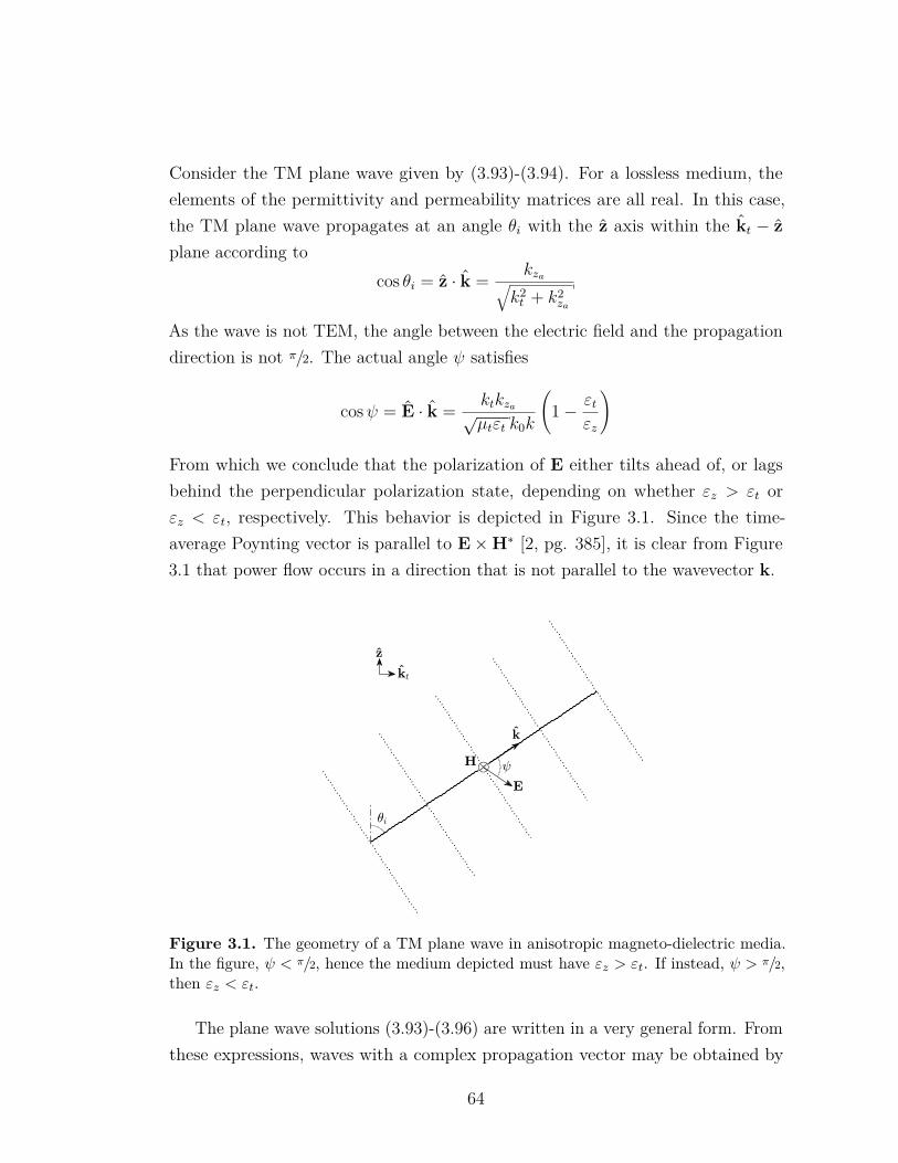
Consider the TM plane wave given by (3.93)-(3.94). For a lossless medium, theelements of the permittivity and permeability matrices are all real. In this case,the TM plane wave propagates at an angle θi with the z axis within the kt − zplane according to

cos θi = z · k = kza√k2t + k2

za

As the wave is not TEM, the angle between the electric field and the propagationdirection is not π/2. The actual angle ψ satisfies

cosψ = E · k = ktkza√µtεt k0k

(1− εt

εz

)

From which we conclude that the polarization of E either tilts ahead of, or lagsbehind the perpendicular polarization state, depending on whether εz > εt orεz < εt, respectively. This behavior is depicted in Figure 3.1. Since the time-average Poynting vector is parallel to E×H∗ [2, pg. 385], it is clear from Figure3.1 that power flow occurs in a direction that is not parallel to the wavevector k.

Figure 3.1. The geometry of a TM plane wave in anisotropic magneto-dielectric media.In the figure, ψ < π/2, hence the medium depicted must have εz > εt. If instead, ψ > π/2,then εz < εt.

The plane wave solutions (3.93)-(3.96) are written in a very general form. Fromthese expressions, waves with a complex propagation vector may be obtained by

64

substitution of various values for kt. For instance, a TM plane wave in cutoff ischaracterized by the condition

kt >√µtεz k0 (3.97)

In this case, e−jkzaz = e−αz, where

α =√εtεzk2t − µtεtk2

0 (3.98)

The complex propagation vector in this case is k = kt− zjα. Later, when modelingpropagation of surface waves in a grounded anisotropic magneto-dielectric substrate,we assume the wave in the air region above the substrate is in cutoff with respectto z, i.e. kt > k0, so that propagation occurs tangential to the substrate, and sothat field amplitudes exponentially decrease at large distances from the substrate,implying a tightly confined wave. We insist, however, that the wave inside thesubstrate is not in cutoff with respect to z, hence kt <

√µtεz k0. We readily

conclude, without detailed consideration of the underlying boundary value problem,that for TM surface waves to propagate in the anisotropic substrate, kt must satisfy

k0 < kt <√µtεz k0 (3.99)

A similar analysis applies to TE plane waves. Surface waves in anisotropic magneto-dielectric substrates are considered in more detail in Section 3.3.

3.2.4 Hybrid Mode Wave Propagation for Arbitrary Directionsof Propagation

Plane waves not propagating along principal axes or within principal planesof the anisotropic magneto-dielectric medium are considerably more complicated,and less familiar in their physical properties. Waves propagating at an angle withrespect to all three principal axes of the anisotropic medium are neither TE, norTM to the direction of propagation.

From a computational standpoint, there is little advantage to working withthe explicit analytical expressions for the plane waves. In fact, (3.22) is in a form

65

convenient for computation of waves propagating in arbitrary directions5

eig(W) =[QEt

Λ]

The eigenvalues p1 and p2 of W can be easily extracted from the Λ matrix onceit has been computed. However, to gain some insight, an analytical formula maybe given for both eigenvalues. Using the methods outlined in previous sections, theformula obtained is

p1,2 = 12

(εxεz

+ µxµz

)k2x +

(εyεz

+ µyµz

)k2y − (µxεy + εxµy)k2

0

±1

4

(εxεz− µxµz

)k2x +

(εyεz− µyµz

)k2y + (µxεy − εxµy)k2

0

2

+

(εxεz− µxµz

)(εyεz− µyµz

)k2xk

2y

1/2

(3.100)

where the 1, 2 subscripts for the eigenvalues correspond to +,− in the formula,respectively. Firstly, we observe from (3.100) the tremendous increase in complexityfor the eigenvalues, compared to plane waves propagating along principal axes orplanes. A second, important observation is that the eigenvalues themselves may becomplex over a certain band of frequencies, i.e. p = pr + jpi. Interestingly, a singleplane wave with a complex eigenvalue carries power that diminishes as the wavepropagates, even though the elements of the permittivity and permeability could bepurely real. The decrease of power normally implies a loss of energy to dissipativeprocesses in the material, but there are no physical energy-loss mechanisms in amedium with purely real permittivity and permeability. Nevertheless, complexwaves computed using (3.22) solve Maxwell’s equations, and as a consequencethey satisfy the mathematical statement of Poynting’s theorem. This follows sincePoynting’s theorem can be derived from Maxwell’s equations.

For lossless media, according to (3.100), if the eigenvalues are complex, thenthey must be the complex conjugate of each other. When this is true, it can beshown that the eigenvectors are also complex conjugates. If both types of complexwaves are excited with complex conjugate amplitudes, then their sum leads to

5In MATLAB, the syntax for the calculation indicated by (3.22) is simply[Q,L] = eig(W);

66

transverse electric fields of the form (E0ve−√p z + E∗0v∗e−

√p∗ z) which are purely

real-valued, regardless of the particular values of v or p. From this fact, it ispossible to show that the time-average Poynting vector of the sum of both complexwaves is perpendicular to z. Thus the total complex wave comprising the twoindividual conjugate waves is effectively in cutoff. For pairs of complex modeswith arbitrary amplitudes, the lack of power orthogonality can be associated withsome interesting theorems regarding the conversion of power between modes. Forthe case of a closed, isotropic, lossless waveguide, the power conversion propertiesamong complex modes has been derived using the Lorentz reciprocity theorem [52].For waveguides filled with gyrotropic material, the relationships between powerflow and stored electric and magnetic energies for a single complex mode havebeen given [53]. It remains to determine the power/energy conversion propertiesamong pairs of complex modes in an anisotropic magneto-dielectric medium. Aninitial investigation of the complex modes propagating in a rectangular conductingwaveguide filled homogeneously with anisotropic magneto-dielectric media wasgiven recently by the author [21].

An additional peculiarity arising from a complex propagation constant is thepossibility for backward wave propagation. A backward wave is characterized by apropagation coefficient α + jβ where α and β have opposite signs. The possibilityfor backward wave complex modes has been noticed before, in guided wave modeson dielectric rods [54].

We give the following numerical example, to illustrate some of the propertiesdescribed above. Assume kx = ky = 20π, and set εx = 2, εy = 4, εz = 15, µx = 8,µy = 3, µz = 17. We define the propagation coefficients αi and βi according to√pi = αi + jβi. The values of the coefficients versus k0 are shown in Figure 3.2.In Figure 3.2, the propagation coefficients are complex valued approximately

when 6.8 < k0 < 21.9. Over this range, the propagation coefficients of the twotypes of plane waves are complex conjugates, as claimed. Over the same interval,the plane wave labeled in Figure 3.2 with the subscript 2 exhibits backward wavebehavior.

67

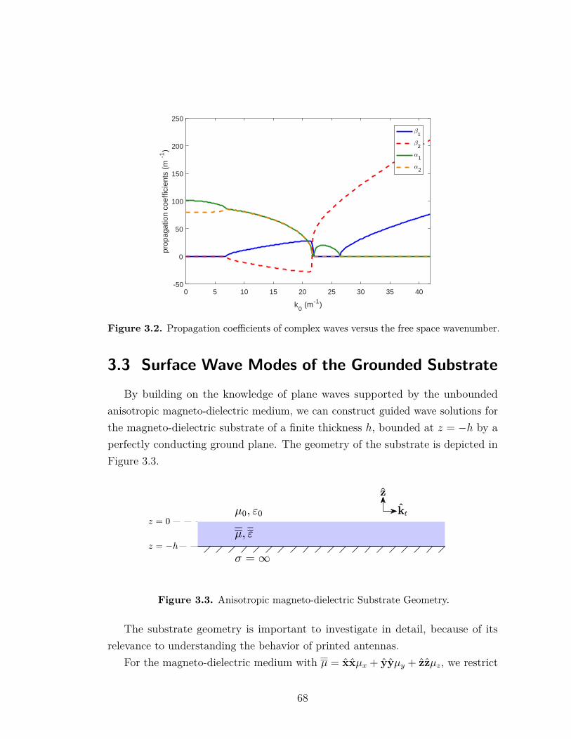
0 5 10 15 20 25 30 35 40

k0 (m-1)

-50

0

50

100

150

200

250

prop

agat

ion

coef

ficie

nts

(m-1

)

1

2

1

2

Figure 3.2. Propagation coefficients of complex waves versus the free space wavenumber.

3.3 Surface Wave Modes of the Grounded SubstrateBy building on the knowledge of plane waves supported by the unbounded

anisotropic magneto-dielectric medium, we can construct guided wave solutions forthe magneto-dielectric substrate of a finite thickness h, bounded at z = −h by aperfectly conducting ground plane. The geometry of the substrate is depicted inFigure 3.3.

Figure 3.3. Anisotropic magneto-dielectric Substrate Geometry.

The substrate geometry is important to investigate in detail, because of itsrelevance to understanding the behavior of printed antennas.

For the magneto-dielectric medium with µ = xxµx + yyµy + zzµz, we restrict

68

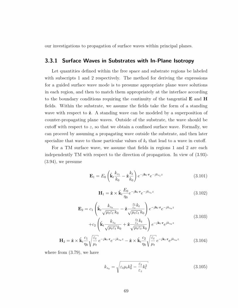
our investigations to propagation of surface waves within principal planes.

3.3.1 Surface Waves in Substrates with In-Plane Isotropy

Let quantities defined within the free space and substrate regions be labeledwith subscripts 1 and 2 respectively. The method for deriving the expressionsfor a guided surface wave mode is to presume appropriate plane wave solutionsin each region, and then to match them appropriately at the interface accordingto the boundary conditions requiring the continuity of the tangential E and Hfields. Within the substrate, we assume the fields take the form of a standingwave with respect to z. A standing wave can be modeled by a superposition ofcounter-propagating plane waves. Outside of the substrate, the wave should becutoff with respect to z, so that we obtain a confined surface wave. Formally, wecan proceed by assuming a propagating wave outside the substrate, and then laterspecialize that wave to those particular values of kt that lead to a wave in cutoff.

For a TM surface wave, we assume that fields in regions 1 and 2 are eachindependently TM with respect to the direction of propagation. In view of (3.93)-(3.94), we presume

E1 = E0

(ktkz1

k0− z

ktk0

)e−jkt·re−jkz1z (3.101)

H1 = z× ktE0

η0e−jkt·re−jkz1z (3.102)

E2 = c1

ktkza√µtεt k0

− zεt

εzkt

√µtεt k0

e−jkt·re−jkzaz

+c2

ktkza√µtεt k0

+ zεt

εzkt

√µtεt k0

e−jkt·rejkzaz

(3.103)

H2 = z× ktc1

η0

√εtµte−jkt·re−jkzaz − z× kt

c2

η0

√εtµte−jkt·rejkzaz (3.104)

where from (3.79), we have

kza =√εtµtk2

0 −εtεzk2t (3.105)

69

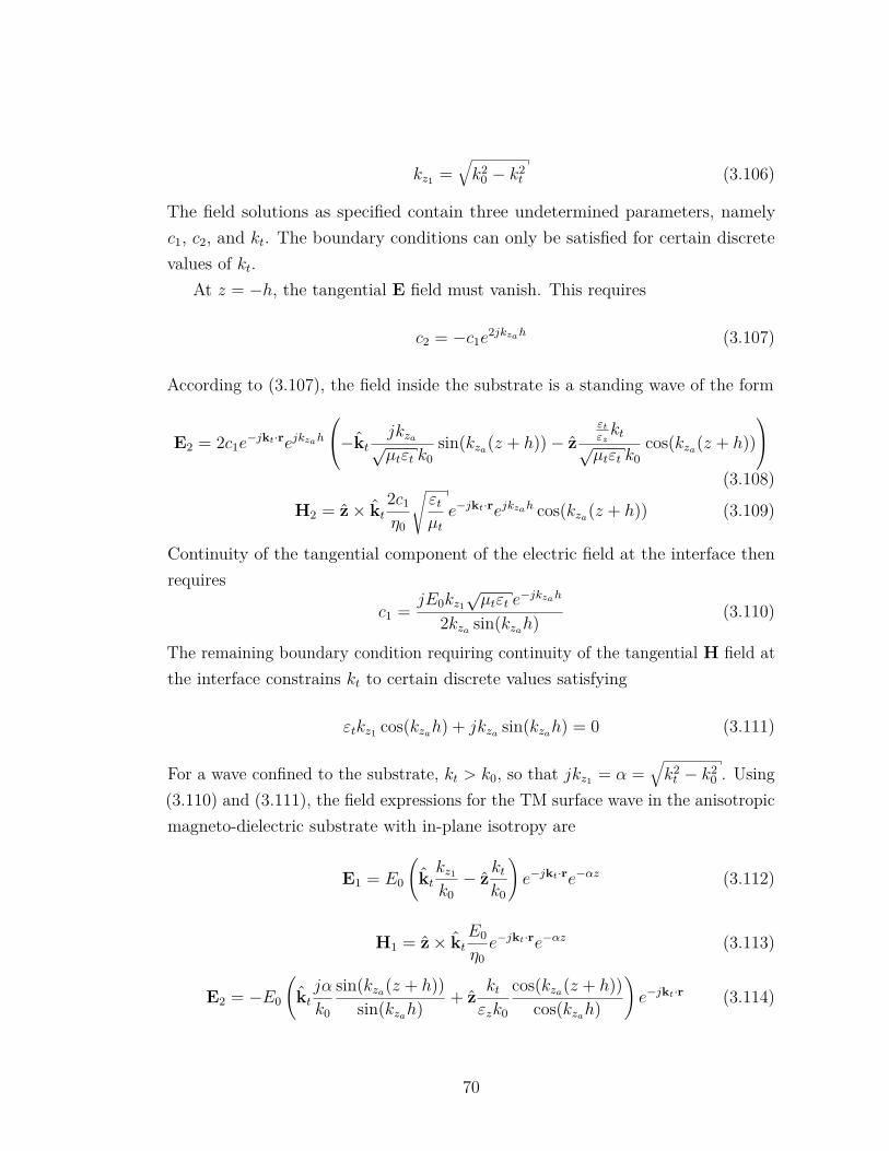
kz1 =√k2

0 − k2t (3.106)

The field solutions as specified contain three undetermined parameters, namelyc1, c2, and kt. The boundary conditions can only be satisfied for certain discretevalues of kt.

At z = −h, the tangential E field must vanish. This requires

c2 = −c1e2jkzah (3.107)

According to (3.107), the field inside the substrate is a standing wave of the form

E2 = 2c1e−jkt·rejkzah

−ktjkza√µtεt k0

sin(kza(z + h))− zεt

εzkt

√µtεt k0

cos(kza(z + h))

(3.108)

H2 = z× kt2c1

η0

√εtµte−jkt·rejkzah cos(kza(z + h)) (3.109)

Continuity of the tangential component of the electric field at the interface thenrequires

c1 =jE0kz1

√µtεt e

−jkzah

2kza sin(kzah) (3.110)

The remaining boundary condition requiring continuity of the tangential H field atthe interface constrains kt to certain discrete values satisfying

εtkz1 cos(kzah) + jkza sin(kzah) = 0 (3.111)

For a wave confined to the substrate, kt > k0, so that jkz1 = α =√k2t − k2

0 . Using(3.110) and (3.111), the field expressions for the TM surface wave in the anisotropicmagneto-dielectric substrate with in-plane isotropy are

E1 = E0

(ktkz1

k0− z

ktk0

)e−jkt·re−αz (3.112)

H1 = z× ktE0

η0e−jkt·re−αz (3.113)

E2 = −E0

(ktjα

k0

sin(kza(z + h))sin(kzah) + z

ktεzk0

cos(kza(z + h))cos(kzah)

)e−jkt·r (3.114)

70

H2 = z× ktE0

η0e−jkt·r cos(kza(z + h))

cos(kzah) (3.115)

Combining (3.105) and (3.111), the dispersion equation governing kt is

−εt cosh√εtµtk2

0 −εtεzk2t

√k2t − k2

0 +sinh√εtµtk2

0 −εtεzk2t

√εtµtk20 −

εtεzk2t = 0

(3.116)At a given radian frequency ω, the free-space wavenumber k0 is determined, andhence (3.116) becomes an equation implicitly specifying the propagation coefficientsof surface waves as a function of frequency.

To make (3.116) unambiguous, we must first define the the square root func-tion kz1 =

√k2

0 − k2t appearing in (3.116).6 For proper modes that do not grow

exponentially, we require the imaginary part of kz1 to be negative. For an arbitrarycomplex input w, the square root function can be suitably defined as

√w = −

√|w| ejθ/2

where θ is the phase angle of w taken from the interval (0, 2π]. It can be verifiedthat for any value of θ taken over the given interval, that the imaginary part of√w is never positive.As is known for isotropic substrates [55, pg. 697], for a given frequency, and

adopting our definition of kz1 , then only a finite number of proper surface wavemodes exist in the anisotropic substrate. This is different than closed wave guides,where an infinite number of modes are possible at every frequency, though somewould be in cutoff and thus non-propagating. In an open surface wave guidingstructure, rather than a surface wave merely transitioning from propagating to non-propagating at cutoff, it transitions from proper to improper, and hence effectivelyfrom existence to non-existence.7 This implies for an impressed excitation of surface

6The precise definition of kza is unimportant since a change of sign on kza makes no differencein (3.116).

7The improper surface wave modes are called leaky-wave modes [55, pp.718,732-734]. Theygrow exponentially in the +z direction, and decay exponentially along kt. Though the modes areimproper, within a small angular region in space over the substrate, the competing exponentialattenuation and growth factors lead to a small amount of exponential attenuation along the radialdirection. As a result, it has been found in the approximate expansion of radiation fields, thatleaky wave modes are sometimes relevant. In these expansions the field observed at each anglewith respect to the source is separately and independently expanded, and only at observationangles where the leaky wave does not exponentially grow radially from the source will the leaky

71

waves in a substrate, for example through the electric currents associated withan antenna, that for a continuous solution as a function of frequency, it must bethat the surface wave is excited at progressively smaller amplitudes as cutoff isapproached. We conclude that for a given source of known operating frequency, thecutoff frequencies are an important factor in determining the relative significanceof particular surface wave modes.

Equation (3.111) is transcendental in kt, admitting no algebraic solution [55, pp.713-715]. As written, the equation is of the form A + B = 0. The only intervalfor kt over which the two factors could possibly cancel is when both factors arepurely real. This implies k0 < kt. Furthermore, one term must be positive and theother negative. For kt >

√µtεz k0, the right hand term becomes negative, while

the left hand term also remains negative. The sum of two negative terms is neverzero. Thus we require

k0 < kt <√µtεz k0 (3.117)

Equation (3.117) agrees with (3.99), which was obtained through an analysis ofcutoff conditions for plane waves. Now carrying our analysis further, we observewithin this interval for kt, that the cos(kzah) and sin(kzah) trigonometric functionscontrol the sign on both factors. The two terms will only have opposite signs,permitting a solution, when

nπ < hkza < nπ + π

2 (3.118)

where n is any positive integer. For each value of n, there is only one possiblesolution lying in the given interval. For values of n higher than a certain integerN , it will become impossible to find a value of hkza satisfying (3.118) that isconsistent with (3.117). This limits the number of existent surface wave modes fora given frequency to N . As the operating frequency is increased, k0, and hence kza

increases, indicating that (3.118) can be satisfied for higher values of n. Therefore,we can conclude that the number of existent surface wave modes increases as theoperating frequency increases. This implies the existence of cutoff frequencies foreach additional mode, which can be arranged into an ordered set. The modes canbe numbered with a letter n, and the collection of surface wave modes can bedelineated as the TMn modes.

wave contribute [55, pp.739-740].

72

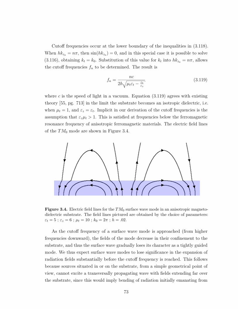
Cutoff frequencies occur at the lower boundary of the inequalities in (3.118).When hkza = nπ, then sin(hkza) = 0, and in this special case it is possible to solve(3.116), obtaining kt = k0. Substitution of this value for kt into hkza = nπ, allowsthe cutoff frequencies fn to be determined. The result is

fn = nc

2h√µtεt − εt

εz

(3.119)

where c is the speed of light in a vacuum. Equation (3.119) agrees with existingtheory [55, pg. 713] in the limit the substrate becomes an isotropic dielectric, i.e.when µt = 1, and εz = εt. Implicit in our derivation of the cutoff frequencies is theassumption that εzµt > 1. This is satisfied at frequencies below the ferromagneticresonance frequency of anisotropic ferromagnetic materials. The electric field linesof the TM0 mode are shown in Figure 3.4.

Figure 3.4. Electric field lines for the TM0 surface wave mode in an anisotropic magneto-dielectric substrate. The field lines pictured are obtained by the choice of parameters:εt = 5 ; εz = 6 ; µt = 10 ; k0 = 2π ; h = .02.

As the cutoff frequency of a surface wave mode is approached (from higherfrequencies downward), the fields of the mode decrease in their confinement to thesubstrate, and thus the surface wave gradually loses its character as a tightly guidedmode. We thus expect surface wave modes to lose significance in the expansion ofradiation fields substantially before the cutoff frequency is reached. This followsbecause sources situated in or on the substrate, from a simple geometrical point ofview, cannot excite a transversally propagating wave with fields extending far overthe substrate, since this would imply bending of radiation initially emanating from

73

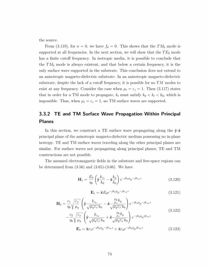
the source.From (3.119), for n = 0, we have f0 = 0. This shows that the TM0 mode is

supported at all frequencies. In the next section, we will show that the TE0 modehas a finite cutoff frequency. In isotropic media, it is possible to conclude thatthe TM0 mode is always existent, and that below a certain frequency, it is theonly surface wave supported in the substrate. This conclusion does not extend toan anisotropic magneto-dielectric substrate. In an anisotropic magneto-dielectricsubstrate, despite the lack of a cutoff frequency, it is possible for no TM modes toexist at any frequency. Consider the case when µt = εz = 1. Then (3.117) statesthat in order for a TM mode to propagate, kt must satisfy k0 < kt < k0, which isimpossible. Thus, when µt = εz = 1, no TM surface waves are supported.

3.3.2 TE and TM Surface Wave Propagation Within PrincipalPlanes

In this section, we construct a TE surface wave propagating along the y-zprincipal plane of the anisotropic magneto-dielectric medium possessing no in-planeisotropy. TE and TM surface waves traveling along the other principal planes aresimilar. For surface waves not propagating along principal planes, TE and TMconstructions are not possible.

The assumed electromagnetic fields in the substrate and free-space regions canbe determined from (3.56) and (3.65)-(3.66). We have

H1 = E0

η0

(ykz1

k0− z

kyk0

)e−jkyye−jkz1z (3.120)

E1 = xE0e−jkyye−jkz1z (3.121)

H2 = c1

η0

√εxµy

ykza√µyεx k0

− zµy

µzky

√µyεx k0

e−jkyye−jkzaz

− c2

η0

√εxµy

ykza√µyεx k0

+ zµy

µzky

√µyεx k0

e−jkyyejkzaz

(3.122)

E2 = xc1e−jkyye−jkzaz + xc2e

−jkyyejkzaz (3.123)

74

where from (3.56),

kza =√εxµyk2

0 −µyµzk2y (3.124)

kz1 =√k2

0 − k2y (3.125)

At z = −h the electric field must vanish. This requires

c2 = −c1e2jkzah

Enforcing continuity on the E and H fields at the interface at z = 0 then leads to

c1 = jE0e−jkzah

2 sin(kzah)

and the dispersion equation for the propagation coefficient ky

jµykz1 sin(kzah) + kza cos(kzah) = 0 (3.126)

Using these results, it is possible to write the surface wave fields within the substratein the form

E2 = xE0e−jkyy

sin(kza(z + h))sin(kzah) (3.127)

H2 = E0

η0e−jkyy

(ykz1

k0

cos(kza(z + h))cos(kzah) − z

kyµzk0

sin(kza(z + h))sin(kzah)

)(3.128)

In order to find the cutoff frequencies, we first deduce from (3.126) that ky mustsatisfy the inequalities

k0 < ky <√εxµz k0 (3.129)

(n+ 12)π < kzah < (n+ 1)π (3.130)

where n is a positive integer, and also delimits the mode number. The cutofffrequencies occur at the lower boundaries of (3.129)-(3.130), from which we obtain

fn =(n+ 1

2)c2h√εxµy − µy

µz

(3.131)

Examining (3.131), we observe that the lowest order TE mode has a nonzero cutofffrequency. Below f0, no TE surface waves exist in the anisotropic substrate within

75

the y-z plane. The magnetic field lines for the TE0 mode are shown in Figure 3.5.

Figure 3.5. Magnetic field lines for the TE0 surface wave mode in an anisotropicmagneto-dielectric substrate. The field lines pictured are obtained for: εx = 10 ; µz = 6 ;µy = 5 ; k0 = 4π ; h = .02.

A similar situation exists for TE surface wave propagation within the x-z plane.Our derivations show that the dispersion equation for the TE surface wave in thex-z principal plane is instead

jµxkz1 sin(kzdh) + kzd

cos(kzdh) = 0 (3.132)

where, according to (3.72),

kzd=√εyµxk2

0 −µxµzk2x (3.133)

The cutoff frequencies are now

fn =(n+ 1

2)c2h√εyµx − µx

µz

(3.134)

From this sampling of 2 possible propagational planes, we infer that the surface wavesatisfies a more general dispersion equation that is a function of the propagationdirection. An important implication is that a cylindrical surface wave, which isguided laterally outward from an interior point of origin, will be spatially dispersive,propagating radially with a non-uniform azimuthally dependent phase velocity.

76

Chapter 4 |Electromagnetic Radiation in thePresence of an AnisotropicMagneto-dielectric Substrate

In Chapter 1, we indicated how anisotropic magneto-dielectric media offerunique possibilities for the design of novel antennas. As in [4], we doubt thatsignificant gains in the performance of antennas can be achieved by any furthermanipulations of purely metal antenna geometries. Any signifant advances thatoccur, we can expect to be earned through the utilization of novel polarizationand magnetization responses of specifically engineered materials. Recent theoret-ical [4] [56] and empirical studies [3] [57] provide evidence that incorporation ofmaterials with isotropic, or anisotropic magneto-dielectric properties can lead tonovel antenna designs exhibiting either advantageous form factors, or desirableradiation polarization and gain patterns.

Of course, many of the theorems that bound the performance of antennas withinthe gain-bandwidth-size tradespace, such as the Chu limit [5], still apply. But thesetheorems have relatively little to say about antennas of intermediate size, or ofantennas whose physical size is constrained, primarily, along one dimension only.

In this chapter, we develop a theory for the calculation of the electromagneticfields associated with arbitrary electric current densities lying over an anisotropicmagneto-dielectric antenna substrate. A primary goal of the previous chapter wasto formulate the expressions for various plane wave functions and guided waves inthe anisotropic magneto-dielectric antenna substrate, for the purpose of enablingexpansions of the radiation fields of planar antenna geometries. Mathematically,

77

the problem is formulated in terms of impressed electric current densities, that arepresumed to flow on the surface of printed planar metallic structures lying overthe substrate. Subsequently, it would then be desirable to formulate the antennaitself as a boundary value problem, enforcing the requirement that the tangentialelectric field be zero everywhere on the surface of the conducting antenna element.However, we must first be able to precisely calculate the radiated fields from agiven presumed current distribution. This is a prerequisite to developing a generalmethod of moments computer program to solve the antenna problem [58]. InChapter 5, the theory we develop is utilized to construct a method of momentsalgorithm for the investigation of thin microstrip dipoles lying over an anisotropicmagneto-dielectric substrate.

While highly general theoretical algorithms have been given for the radiation ofimpressed current distributions within layered anisotropic media [16], they do notimmediately lend themselves to clear physical interpretation, to accurate numericalcalculations of the radiation and surface wave fields, or to numerically stableformulations of the dyadic Green’s functions for use in a method of moments solverfor induced current densities on antennas. Notably, in the spectral expansion ofradiation fields in layered isotropic media, it is well understood how to separate theradiation into physically relevant components, including surface waves, radiatingwaves, leaky waves, and evanescent waves associated with energy storage by theantenna. The general algorithms are a great starting point for the analysis of theunderlying electromagnetic boundary value problems, yet it is clear that thereis immense value in engaging in a more detailed and specific study of variouscases. Considerable physical insight can be gained by proceeding further into theanalytical details of specific problems.

Along these lines, comparatively less general, but more detailed studies ofelectrically biaxial, and of gyrotropic antenna substrates have recently been con-ducted [17] [18] [59]. The adhoc method of calculation of radiation fields from currentsources in the presence of anisotropic material layers that is utilized in [17] [59] isto superpose appropriate scattered fields with an initially radiated field calculatedfrom a study of a source in unbounded media. This approach is workable, butleads to analytical formulations that are seemingly, at intermediate steps, morecomplicated than necessary. A simpler method, that we apply here, is to formulategeneral solutions for the fields in each layer of the problem geometry in terms of a

78

set of unknown coefficients, and then to calculate the values of those coefficients fora given source current distribution through the application of boundary conditions.

In this chapter, dyadic Green’s functions are derived for the electromagneticradiation from arbitrary current sources lying over the surface of an anisotropicmagneto-dielectric antenna substrate that is in-plane isotropic. We extract formulasfor the radiation fields by the asymptotic stationary phase method, and for thesurface wave fields using Cauchy’s residue theorem.

For the case of no in-plane isotropy, we focus on polarization rotation effects,and other novel features. We will often constrain observation points such thatsimple formulas may be obtained, from which we can arrive at some interestingand useful conclusions. In particular, the theory indicates the intriguing possibilityof developing novel, compact, circularly polarized antennas.

4.1 The Plane Wave Spectrum, and Formulation ofthe Green’s Function Problem

For an impressed current distribution J, Maxwell’s equations, along with anyboundary conditions appropriate to the physical geometry under consideration,completely determine the E and H fields. The two curl equations, including theimpressed current density J, are

∇× E = −jk0η0µ ·H (4.1)

∇×H = Jsδ(z) + jk0

η0ε · E (4.2)

The current distribution Js is a surface current distribution flowing on the anisotropicmagneto-dielectric substrate. In the model, we place the current distribution exactlyat the interface, as shown in Figure 4.1. We presume z · Js = 0.

From a function-theoretic point of view, the two-dimensional surface currentdensity Js, can be expanded in a double Fourier integral according to

Js = 1(2π)2

+∞¨−∞

Jse−jkt·r dkx dky (4.3)

79

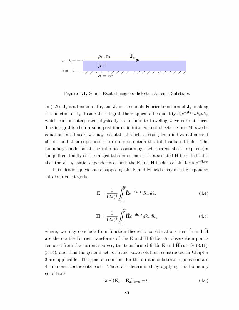
Figure 4.1. Source-Excited magneto-dielectric Antenna Substrate.

In (4.3), Js is a function of r, and Js is the double Fourier transform of Js, makingit a function of kt. Inside the integral, there appears the quantity Jse−jkt·rdkxdky,which can be interpreted physically as an infinite traveling wave current sheet.The integral is then a superposition of infinite current sheets. Since Maxwell’sequations are linear, we may calculate the fields arising from individual currentsheets, and then superpose the results to obtain the total radiated field. Theboundary condition at the interface containing each current sheet, requiring ajump-discontinuity of the tangential component of the associated H field, indicatesthat the x− y spatial dependence of both the E and H fields is of the form e−jkt·r.

This idea is equivalent to supposing the E and H fields may also be expandedinto Fourier integrals.

E = 1(2π)2

+∞¨−∞

Ee−jkt·r dkx dky (4.4)

H = 1(2π)2

+∞¨−∞

He−jkt·r dkx dky (4.5)

where, we may conclude from function-theoretic considerations that E and Hare the double Fourier transforms of the E and H fields. At observation pointsremoved from the current sources, the transformed fields E and H satisfy (3.11)-(3.14), and thus the general sets of plane wave solutions constructed in Chapter3 are applicable. The general solutions for the air and substrate regions contain4 unknown coefficients each. These are determined by applying the boundaryconditions

z× (E1 − E2)|z=0 = 0 (4.6)

80

z× (H1 − H2)|z=0 = Js (4.7)

z× E2|z=−h = 0 (4.8)

Furthermore, we require the fields to be proper in the free-space region. Thisrequires that only waves with a e−jkz1z dependence should be included in theFourier integral for E1 and H1. Otherwise, waves for which kt > k0 would growexponentially in the +z direction. Subject to this additional constraint, (4.6)-(4.8)become a linear system of 6 equations in the 6 remaining unknown coefficients.

The solution of (4.6)-(4.8) enables the matrices GE1,2 , GH1,2 to be defined suchthat

E1,2 = GE1,2 · Js (4.9)

H1,2 = GH1,2 · Js (4.10)

The matrices GE1,2 , GH1,2 are called the spectral dyadic Green’s functions. Thevarious field quantities are therefore determined from integral expressions of theform

E = 1(2π)2

+∞¨−∞

GE · Jse−jkt·r dkx dky

which upon replacing Js with the double Fourier transform of Js, is equivalent to

E = 1(2π)2

+∞¨−∞

GE ·

+∞¨−∞

Jsejkt·r′

dx′dy′

e−jkt·r dkx dky

E = 1(2π)2

+∞¨−∞

+∞¨−∞

GEe−jkt·(r−r′ ) dkx dky

· Js dx′ dy′The bracketed quantity is the spatial dyadic Green’s function.

GE = 1(2π)2

+∞¨−∞

GEe−jkt·(r−r′ ) dkx dky (4.11)

We concern ourselves primarily with determining the spectral dyadic Green’sfunctions. The spatial dyadic Green’s function is considered only for the asymptotic

81

evaluation of the radiation fields into the free space region.

4.2 Dyadic Green’s Functions for Substrate with In-Plane Isotropy

Examining (4.6)-(4.8), we observe that only the components of the field tan-gential to the air-substrate interface are involved in the boundary conditions. Itis therefore convenient to formulate, and solve for the unknown coefficients thatdetermine the radiated fields, in terms of the tangential field components alone.In the free space region over the substrate, the general solution for the tangentialfields Et1 and Ht1 is given by (3.23) and (3.25) as

Et1 = QEt1· c1e

−jkz1z (4.12)

Ht1 = −QHt1· c1e

−jkz1z (4.13)

wherekz1 =

√k2

0 − k2t (4.14)

QEt1=[kt z× kt

](4.15)

QHt1= 1η0

[− k0kz1

z× ktkz1k0

kt]

(4.16)

and c1 is a vector of 2 unknown coefficients. In the substrate, the general solutionis

Et2 = QEt2· e−Λ

1/2z · c+ + QEt2

· eΛ1/2z · c− (4.17)

Ht2 = −QHt2· e−Λ

1/2z · c+ + QHt2

· eΛ1/2z · c− (4.18)

whereΛ = −xxk2

za− yyk2

zb(4.19)

kza =√εtµtk2

0 −εtεzk2t (4.20)

kzb=√εtµtk2

0 −µtµzk2t (4.21)

QEt2=[kt z× kt

](4.22)

82

QHt2= 1η0

[− εtk0

kzaz× kt

kzb

µtk0kt]

(4.23)

The boundary condition requiring the tangential electric field to vanish at theconducting ground plane at z = −h yields

c− = −e2Λ1/2h · c+ (4.24)

Substitution of (4.24) into (4.17)-(4.18) yields

Et2 = −2QEt2· sinh(Λ

1/2(z + h)) · eΛ

1/2h · c+ (4.25)

Ht2 = −2QHt2· cosh(Λ

1/2(z + h)) · eΛ

1/2h · c+ (4.26)

These expressions can be simplified by introducing a new set of unknown coefficientsdefined as

c2 = −2eΛ1/2h · c+ (4.27)

So that the general solution in the substrate region may be concisely represented by

Et2 = QEt2· sinh(Λ

1/2(z + h)) · c2 (4.28)

Ht2 = QHt2· cosh(Λ

1/2(z + h)) · c2 (4.29)

The remaining boundary conditions at the interface with the current sheet Jsrequire

c1 − sinh(Λ1/2h) · c2 = 0 (4.30)

QHt1· c1 + QHt2

· cosh(Λ1/2h) · c2 = z× Js (4.31)

We can quickly solve (4.30) for c1, and substitute the result into (4.31). This leadsto a matrix equation for c2,

QHt1· sinh(Λ

1/2h) · c2 + QHt2

· cosh(Λ1/2h) · c2 = z× Js (4.32)

It is then useful to introduce a new matrix M, defined by

M = xxεtkz1

kza

+ yykzb

µtkz1

(4.33)

83

From this definition, it follows that

QHt2= QHt1

·M (4.34)

Substitution of (4.34) into (4.32) yields

QHt1· S · c2 = z× Js (4.35)

whereS = sinh(Λ

1/2h) + M · cosh(Λ

1/2h) (4.36)

Hence, we may write the solution in the form

c2 = S−1·Q−1Ht1· z× Js (4.37)

We introduce yet another new matrix Z1, equal to 1

Z1 = η0

(xx

kz1

k0+ yy

k0

kz1

)(4.38)

Using this matrix, we can write

QHt1=[−z× kt kt

]· Z−11 (4.39)

Thus

Q−1Ht1

= Z1 ·[−z× kt kt

]−1= Z1 ·

−z× ktkt

(4.40)

1We have, at this point, elected to introduce a number of matrices. Each matrix introduced hasphysical significance. Z1 is the diagonal matrix whose diagonal entries are the wave impedancesfor TM and TE waves in free-space [2, eqs. 10-31,10-54]. The analogous matrix Z2 for thesubstrate region can also be defined. It is then possible to show that M = Z1 · Z

−12 . Thus M is

the diagonal matrix whose entries are the ratios of the wave impedances for TE and TM wavesin the free space and substrate regions. Finally, S is the matrix whose diagonal entries are thedispersion equations for TE and TM surface waves supported by the substrate. Hence, when kt isequal to a value that is consistent with a surface wave, one of the entries in S is zero. This is animportant point that we will return to in Section 4.2.2.

84

The cross product operation z× can, for the tangential current sheet, be formulatedas the 2x2 matrix

z× =0 −1

1 0

(4.41)

Thus, combining (4.40) and (4.41), we obtain

Q−1Ht1· z× Js = −Z1 ·

−z× ktkt

·0 −1

1 0

· Js

Q−1Ht1· z× Js = −Z1 ·

ktz× kt

· JsQ−1Ht1· z× Js = −Z1 ·Q

T

Et1· Js (4.42)

where QT

Et1is the transpose of QEt1

. Substitution of (4.42) into (4.37) gives

c2 = −S−1· Z1 ·Q

T

Et1· Js (4.43)

From (4.30), we have

c1 = − sinh(

Λ1/2h

)· S−1· Z1 ·Q

T

Et1· Js (4.44)

By substitution of (4.44) in (4.12), the tangential electric field in the free spaceregion is

Et1 =(QEt1

·D1 ·QT

Et1

)· Js = GE1t

· Js (4.45)

whereD1 = − sinh

(Λ

1/2h

)· S−1· Z1e

−jkz1z (4.46)

We went through a lot of extra work to arrive at (4.45). The significance of the resultfollows once we realize that D1 is a diagonal matrix, since it is formed from theproduct of other diagonal matrices. Hence, (4.45) is the “PDP−1” diagonalizationof the tangential part of the spectral dyadic Green’s function GE1 , denoted GE1t

,that connects Et and Js. This implies that the diagonal entries of D1 are theeigenvalues of GE1t

. It also implies that kt, and z × kt are the eigenvectors ofGE1t

. The expression shows that GE1tprojects the kt component of Js onto the kt

85

component of Et, and the same with z× kt. This is easily seen, if we use (4.45) toexpand GE1t

into a sum of 2 dyads, obtaining

GE1t= −

(ktkt

jη0kzakz1 sin(kzah)k0Tm

+ (z× kt)(z× kt)jη0µtk0 sin(kzb

h)Te

)e−jkz1z

(4.47)where Tm and Te are the dispersion equations for surface wave modes in thesubstrate.

Tm = εtkz1 cos(kzah) + jkza sin(kzah) (4.48)

Te = jµtkz1 sin(kzbh) + kzb

cos(kzbh) (4.49)

The remaining term of the complete Green’s function GE1 may be obtained fromthe tangential part GE1t

using the Maxwell equation ∇ · E1 = 0. This equationrequires

Ez1 = − ktkz1

· Et1 (4.50)

Combining (4.46) and (4.50), we find

GE1 = −jη0k0

((kt −

ktkz1

z)ktkzakz1 sin(kzah)

k20Tm

+ (z× kt)(z× kt)µt sin(kzb

h)Te

)e−jkz1z

(4.51)The other Green’s functions may be derived similarly. They are

GH1 = −jk0

((z× kt)kt

kza sin(kzah)k0Tm

− (kt −ktkz1

z)(z× kt)µtkz1 sin(kzb

h)k0Te

)e−jkz1z

(4.52)

GE2 =− jη0k0

(ktkt

kzakz1 sin(kza(z + h))k2

0Tm+

(z× kt)(z× kt)µt sin(kzb

(z + h))Te

− zktjεtktkz1 cos(kza(z + h))

εzk20Tm

) (4.53)

GH2 =− jk0

((z× kt)kt

jεtkz1 cos(kza(z + h))k0Tm

−

(kt)(z× kt)jkzb

cos(kzb(z + h))

k0Te+ z(z× kt)

µtkt sin(kzb(z + h))

µzk0Te

) (4.54)

These expressions are in a convenient form for theoretical work. They are lesssuitable for the calculation of fields at large distances from the current sources.

86

In this case, it becomes very difficult to accurately evaluate the required inverseFourier transforms. Since the exponential and trigonometric functions containedwithin the expressions for the underlying dyadic Green’s functions become highlyoscillatory for large distance, numerical integration consists of adding up largelycancelling contributions over the majority of the integration interval. Large positiveand negative canceling contributions to the integral become impossible to evalu-ate accurately with a finite relative floating point accuracy on a computer. Forthis reason, we are motivated to perform an asymptotic analysis for the far-fieldradiation.

4.2.1 Asymptotic Evaluation of the Radiation Fieldby Stationary Phase

The stationary phase method is a technique that can be used for the approximateevaluation of inverse double Fourier transforms. In electromagnetics, the methodcan be readily applied to problem geometries where the Fourier transformed elec-tromagnetic fields are specified over a plane at z = 0, and the field at far distancesin the region z > 0 are desired [60]. The Fourier transform of the E field at z = 0in the free space region is

E1(kt, z = 0) = GE1(kt, z = 0) · Js (4.55)

The stationary phase formula for the E far-field is [60, Eq. 12-107]

E1(r) = jk0 cos θE1(kts , z = 0)e−jk0r

2πr (4.56)

where kts is the transverse wavenumber evaluated at the stationary point in k-space,given by

kts = xkxs + ykys (4.57)

kxs = k0 sin θ cosφ (4.58)

kys = k0 sin θ sinφ (4.59)

Utilizing (4.57)-(4.59), the stationary values of other quantities are shown to be

kts = k0 sin θ (4.60)

87

kz1s= k0 cos θ (4.61)

kts = ρ (4.62)

z× kts = φ (4.63)

kzas= k0

√εtµt −

εtεz

sin2 θ (4.64)

kzbs= k0

√εtµt −

µtµz

sin2 θ (4.65)

Additionally, Tes and Tms are the stationary values of the surface wave dispersionequations. These can be obtained by substitution of the above quantities whereappropriate.

Having given the stationary quantities (4.60)-(4.65), it is a simple exercise toshow (4.55) reduces to

E1(kts , z = 0) = −jk0η0

(θρkzas

sin(kzash)

k0Tms

+ φφµt sin(kzbs

h)Tes

)· Js(kts) (4.66)

Substitution of (4.66) into (4.56) yields

E1(r) = k0η0 cos θ(θρkzas

sin(kzash)

Tms

+ φφµtk0 sin(kzbs

h)Tes

)· Js(kts)e

−jk0r

2πr (4.67)

Since z · Js = 0, we have the following equality

ρ cos θ · Js = θ · Js (4.68)

Thus, (4.67) is equivalent to

E1(r) = k0η0

(θθkzas

sin(kzash)

Tms

+ φφµtk0 cos θ sin(kzbs

h)Tes

)· Js(kts)e

−jk0r

2πr (4.69)

The stationary transformed current density, Js(kts), can be written in terms of Jsas

Js(kts) =+∞¨−∞

Js(r′)ejkxsx

′

ejkysy′

dx′dy′ (4.70)

88

and sincekxsx

′ + kysy′ = k0

(x′ sin θ cosφ+ y

′ sin θ sinφ)

kxsx′ + kysy

′ = k0r ·(x′x + y

′y)

kxsx′ + kysy

′ = k0r · r′ (4.71)

we may combine (4.70) and (4.71) to obtain

Js(kts) =+∞¨−∞

Js(r′)ejk0r·r′ dx

′dy′ (4.72)

Substitution of (4.72) into (4.69) yields

E1(r) =+∞¨−∞

k0η0

(θθkzas

sin(kzash)

Tms

+ φφµtk0 cos θ sin(kzbs

h)Tes

)·Js(r

′)e−jk0(r−r·r′ )

2πr dx′dy′

(4.73)From (4.73), the asymptotic form of the spatial dyadic Green’s function is identifiedwith

GE1(r, r′) = k0η0

(θθkzas

sin(kzash)

Tms

+ φφµtk0 cos θ sin(kzbs

h)Tes

)e−jk0(r−r·r′ )

2πr(4.74)

As a verification of these results, in the limit that µ = I (ε is allowed to remainanisotropic), (4.74) agrees with [15, eqs. 20-22].

We can further our confidence in the validity of (4.74) by investigating a numberof limiting cases of theoretical significance. First, consider the limiting case whenthe substrate is set to free space. That is, set µ = ε = I. For free space, we firstobserve that kzas

= kzbs= k0 cos θ. Accordingly, Tes and Tms reduce to

Tms = Tes = k0 cos θejk0h cos θ

Thus, (4.74) indicates that the asymptotic form of the dyadic Green’s function fortangential current sources lying in free space over a perfectly conducting ground

89

plane is

limε,µ→I

GE1(r, r′) = k0η0 sin(k0h cos θ)e−jk0h cos θ(θθ + φφ)e−jk0(r−r·r′ )

2πr (4.75)

This is the correct asymptotic result, as can be verified by application of imagetheory, replacing the PEC ground plane at z = −h with an image source of oppositepolarity located at z = −2h.

To reduce the formula further to the case of a source located in unbounded freespace, it is necessary to suppose the substrate has a small amount of loss, such thatk0 has a small negative imaginary part, as in k0 − jδ. We evaluate the limit

limδ→0h→∞

GE1

Accordingly, we find

limh→∞

sin((k0−jδ)h cos θ) = limh→∞

12j (ej(k0−jδ)h cos θ−e−j(k0−jδ)h cos θ) ∼ 1

2j ej(k0−δ)h cos θ

Then we substitute this result in (4.75), and finally let δ → 0. We obtain theasymptotic form of the free space electric dyadic Green’s function [55, pg. 98]

limδ→0h→∞

GE1(r, r′) = −jk0η0(θθ + φφ)e−jk0(r−r·r′ )

4πr (4.76)

It is interesting to consider the limiting case of a highly magnetic substrate. Welet µt = µz = µr. Then we evaluate the limit

limµr→∞

GE1

To this end, we note that as µr gets very large, quantities approach the variousasymptotic limits

kzas∼ kzbs

∼ k0√εtµt

Tms ∼ jk0√εtµt sin(k0h

√εtµt )

Tes ∼ jµtk0 cos θ sin(k0h√εtµt )

90

Upon replacement of the above quantities with their asymptotic values in theexpression for the dyadic Green’s function, we obtain the asymptotic form of thedyadic Green’s function for a highly magnetic substrate

limµr→∞

GE1(r, r′) = −jk0η0(θθ + φφ)e−jk0(r−r·r′ )

2πr (4.77)

We may conclude from (4.77) that when µr is very large, the substrate acts effectivelylike a perfect magnetic conductor (PMC). In this physical picture, the currentsource lies directly on the PMC, and radiation, according to image theory, is simplydouble that of the free space result. Interestingly, this calculation also shows thatas µr gets very large, the radiation from current sources lying on the substratebecome independent of the substrate thickness h. If only µt →∞, then (4.77) isstill obtained. This implies that a crystal-oriented ferrite substrate, with its highin-plane magnetic permeability (see Figure 2.7), would act somewhat like a PMCbackplane positioned at the source.

To investigate the radiation patterns of antennas, an electric current distributionneeds to be specified. Without formulating a method of moments program, it isdifficult to know the correct form for the current distribution along the conductingelements of an antenna. For certain simple antenna geometries it is possible topresume a sensible current distribution, and to study the resultant radiation. Inparticular, for a very short, linear dipole antenna element of length `, it is customaryto approximate the current distribution as constant. In the extreme limit, we obtaina localized point source, with the current density

Js = a`I0δ(x′)δ(y′) (4.78)

where I0 is the electric current amplitude in amperes. Substitution of (4.78) into(4.73), and integrating over the delta function, we obtain the expected E far-fieldfor a very short dipole antenna

E1(r) = k0η0`I0

(θ(θ · a)kzas

sin(kzash)

Tms

+ φ(φ · a)µtk0 cos θ sin(kzbs

h)Tes

)e−jk0r

2πr(4.79)

When a = x the principal E-plane pattern cut is the x− z plane, and the radiationis θ-directed. The H-plane pattern cut occurs in the y − z plane, and is φ-directed.

91

At θ = 0, both pattern cuts are sampling the same field, and θ for φ = 0 and φ forφ = π

2 are both equal to x. Thus the radiation at θ = 0 is parallel to the currentpolarization.

The E and H-plane patterns for an x-directed short dipole are functions of thefive parameters εt, εz, µt, µz, and h. The relative importance of the permittivityand permeability values depends critically on the the thickness of the substrate.For thin substrates where h is less than 0.4 λ√

µtεt, where λ = c

fis the free-space

wavelength, the radiation patterns are independent of µz, and there is a dependenceon εz for the E-plane pattern only. The patterns are insensitive to µz, primarilybecause the Hz field component must be zero at the PEC ground plane, which fora very thin substrate, would require a rapid spatial variation of Hz in order for Hz

to have non-negligible amplitude within the substrate. When the substrate is thinand not strongly magnetic, there is a substantial effect on the E-plane pattern bythe value εz. However, for µt on the order of εt, there is no subsequent dependenceon εz. Figure 4.2 gives polar log-magnitude plots of E and H-plane patterns forthin substrates with varying electric and magnetic properties.

For h on the order of 0.5 λ√µtεt

, a pattern null arises at θ = 0. As h is in-creased further, additional pattern lobes occur. For h at or near 0.5 λ√

µtεt, the

additional effects of the substrate’s electric and magnetic anisotropy become morepronounced. These anisotropic effects on patterns are diverse and difficult tocharacterize succinctly. We provide a sampling of patterns in Figure 4.3.

The radiation patterns for other types of antennas cannot be analyzed withoutformulating a numerical scheme to determine the induced current densities on theradiating elements. A method of moments algorithm is given in Chapter 5.

4.2.2 Excitation of Surface Waves

In Chapter 3, we showed that the TM0 surface wave is never in cutoff. Weexpect that any impressed current source lying over the magneto-dielectric substratewill deliver a portion of its available power to this wave, which will be carried away,trapped within the substrate. In reality, the antenna substrate is finite, and somefraction of this surface wave power will reach the outer boundary of the substrate,and spill out into the surrounding space. This surface wave leakage will occur ina way that would be difficult to exploit, since the direction and features of the

92

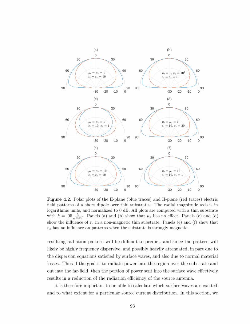
90

60

300

30

60

90-30 -20 -10 0

90

60

300

30

60

90-30 -20 -10 0

90

60

300

30

60

90-30 -20 -10 0

90

60

300

30

60

90-30 -20 -10 0

90

60

300

30

60

90-30 -20 -10 0

90

60

300

30

60

90-30 -20 -10 0

Figure 4.2. Polar plots of the E-plane (blue traces) and H-plane (red traces) electricfield patterns of a short dipole over thin substrates. The radial magnitude axis is inlogarithmic units, and normalized to 0 dB. All plots are computed with a thin substratewith h = .05 λ√

µtεt. Panels (a) and (b) show that µz has no effect. Panels (c) and (d)

show the influence of εz in a non-magnetic thin substrate. Panels (e) and (f) show thatεz has no influence on patterns when the substrate is strongly magnetic.

resulting radiation pattern will be difficult to predict, and since the pattern willlikely be highly frequency dispersive, and possibly heavily attenuated, in part due tothe dispersion equations satisfied by surface waves, and also due to normal materiallosses. Thus if the goal is to radiate power into the region over the substrate andout into the far-field, then the portion of power sent into the surface wave effectivelyresults in a reduction of the radiation efficiency of the source antenna.

It is therefore important to be able to calculate which surface waves are excited,and to what extent for a particular source current distribution. In this section, we

93

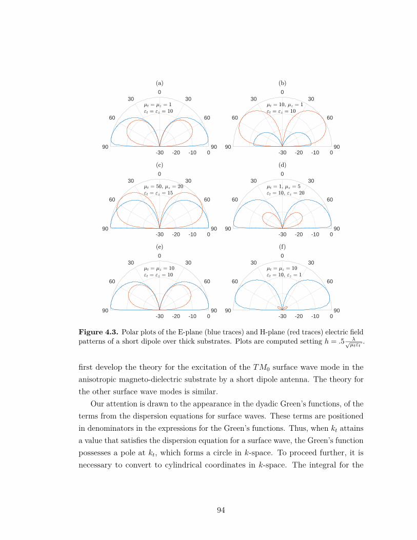
90

60

300

30

60

90-30 -20 -10 0

90

60

300

30

60

90-30 -20 -10 0

90

60

300

30

60

90-30 -20 -10 0

90

60

300

30

60

90-30 -20 -10 0

90

60

300

30

60

90-30 -20 -10 0

90

60

300

30

60

90-30 -20 -10 0

Figure 4.3. Polar plots of the E-plane (blue traces) and H-plane (red traces) electric fieldpatterns of a short dipole over thick substrates. Plots are computed setting h = .5 λ√

µtεt.

first develop the theory for the excitation of the TM0 surface wave mode in theanisotropic magneto-dielectric substrate by a short dipole antenna. The theory forthe other surface wave modes is similar.

Our attention is drawn to the appearance in the dyadic Green’s functions, of theterms from the dispersion equations for surface waves. These terms are positionedin denominators in the expressions for the Green’s functions. Thus, when kt attainsa value that satisfies the dispersion equation for a surface wave, the Green’s functionpossesses a pole at kt, which forms a circle in k-space. To proceed further, it isnecessary to convert to cylindrical coordinates in k-space. The integral for the

94

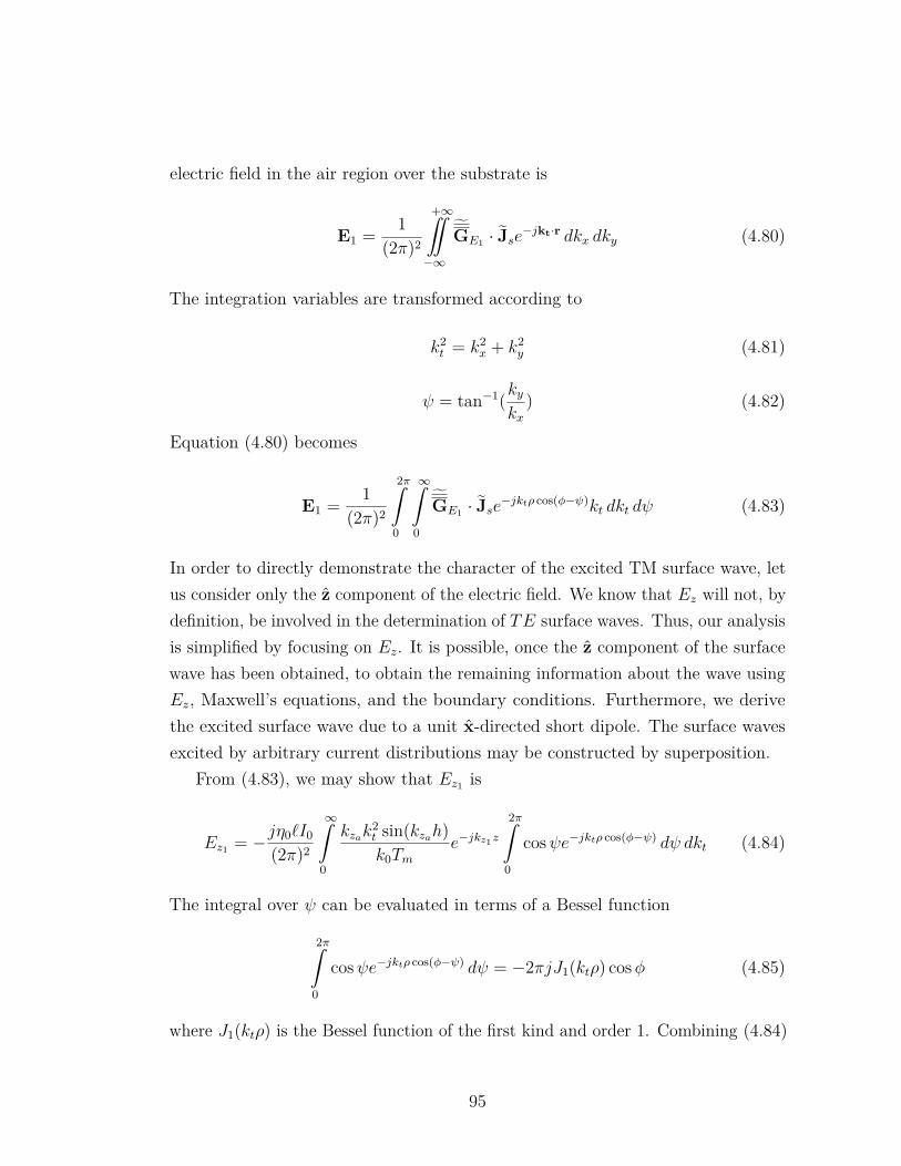
electric field in the air region over the substrate is

E1 = 1(2π)2

+∞¨−∞

GE1 · Jse−jkt·r dkx dky (4.80)

The integration variables are transformed according to

k2t = k2

x + k2y (4.81)

ψ = tan−1(kykx

) (4.82)

Equation (4.80) becomes

E1 = 1(2π)2

2πˆ

0

∞

0

GE1 · Jse−jktρ cos(φ−ψ)kt dkt dψ (4.83)

In order to directly demonstrate the character of the excited TM surface wave, letus consider only the z component of the electric field. We know that Ez will not, bydefinition, be involved in the determination of TE surface waves. Thus, our analysisis simplified by focusing on Ez. It is possible, once the z component of the surfacewave has been obtained, to obtain the remaining information about the wave usingEz, Maxwell’s equations, and the boundary conditions. Furthermore, we derivethe excited surface wave due to a unit x-directed short dipole. The surface wavesexcited by arbitrary current distributions may be constructed by superposition.

From (4.83), we may show that Ez1 is

Ez1 = −jη0`I0

(2π)2

∞

0

kzak2t sin(kzah)k0Tm

e−jkz1z

2πˆ

0

cosψe−jktρ cos(φ−ψ) dψ dkt (4.84)

The integral over ψ can be evaluated in terms of a Bessel function

2πˆ

0

cosψe−jktρ cos(φ−ψ) dψ = −2πjJ1(ktρ) cosφ (4.85)

where J1(ktρ) is the Bessel function of the first kind and order 1. Combining (4.84)

95

and (4.85), we have

Ez1 = −η0`I0

2πk0cosφ

∞

0

kzak2t sin(kzah)Tm

e−jkz1zJ1(ktρ) dkt (4.86)

Using a common trick, we replace J1(ktρ) with 12(H(1)

1 (ktρ) + H(2)1 (ktρ)), where

H(1)1 (ktρ) and H

(2)1 (ktρ) are the Hankel functions of the first and second kind

respectively. Then the integral of H(1)1 (ktρ) over 0 to ∞ may be converted to an

integral over −∞ to 0 of H(2)1 (ktρ) by using a circuit relation [61]. The result is a

single integral over −∞ to ∞. This procedure shows that (4.86) is equivalent to

Ez1 = −η0`I0

4πk0cosφ

∞

−∞

kzak2t sin(kzah)Tm

e−jkz1zH(2)1 (ktρ) dkt (4.87)

The evaluation of the remaining integral yields the total electric field radiated bythe x directed Hertzian dipole. In order to determine the surface wave component,we must adopt the viewpoint that the integral over kt is an integral along thereal axis within the complex kt plane. For points positioned off the real axis, theintegrand in (4.87) is suitably defined according to the theory of functions of acomplex variable. 2

Since all functions in the integrand are analytic, except at poles and branchpoints, we may deform the path of integration off the real axis without changingthe value of the integral. If a closed contour is constructed in the complex kt planethat encloses in a clockwise sense an interior point ktp where the integrand has apole, then the integral around the closed contour is given, according to Cauchy’sresidue theorem, by

−2πjRes(kt = ktp

)(4.88)

where Res(kt = ktp

)is the residue of the integrand at ktp . From a slightly different

perspective, we may deform our contour on the real axis to a different contourthat maintains the same starting and ending points. The original contour plusthe new contour (traversed backward) together form a clockwise closed contour.When the closed contour constructed in this way encloses a pole, we say that the

2Appendix A should be consulted for some background information on complex analysis, as itpertains to (4.87).

96

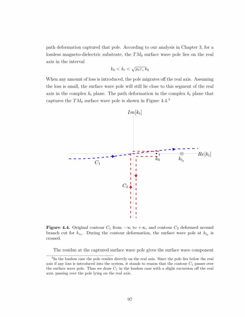
path deformation captured that pole. According to our analysis in Chapter 3, for alossless magneto-dielectric substrate, the TM0 surface wave pole lies on the realaxis in the interval

k0 < kt <√µtεz k0

When any amount of loss is introduced, the pole migrates off the real axis. Assumingthe loss is small, the surface wave pole will still lie close to this segment of the realaxis in the complex kt plane. The path deformation in the complex kt plane thatcaptures the TM0 surface wave pole is shown in Figure 4.4.3

Figure 4.4. Original contour C1 from −∞ to +∞, and contour C2 deformed aroundbranch cut for kz1 . During the contour deformation, the surface wave pole at ktp iscrossed.

The residue at the captured surface wave pole gives the surface wave component3In the lossless case the pole resides directly on the real axis. Since the pole lies below the real

axis if any loss is introduced into the system, it stands to reason that the contour C1 passes overthe surface wave pole. Thus we draw C1 in the lossless case with a slight excursion off the realaxis, passing over the pole lying on the real axis.

97

of the radiated field. We find

Ezsw = jη0`I0

2k0cosφ lim

kt→ktp

(kt − ktp)kzak2t sin(kzah)Tm

e−jkz1zH(2)1 (ktρ)

Ezsw =jη0`I0kzap

k2tp sin(kzap

h)2k0

cosφe−jkz1pzH

(2)1 (ktpρ) lim

kt→ktp

(kt − ktp) 1Tm

Ezsw =jη0`I0kzap

k2tp sin(kzap

h)2k0T

′m

cosφe−jkz1pzH

(2)1 (ktpρ) (4.89)

where T ′m is the derivative of Tm with respect to kt evaluated at ktp . From (4.89),the surface wave can be written as

Ezsw = E0 cosφe−jkz1pzH

(2)1 (ktpρ) (4.90)

where E0 is the amplitude of the wave given by

E0 =jη0`I0kzap

k2tp sin(kzap

h)2k0T

′m

(4.91)

It remains to evaluate the deformed contour that runs around the branch cut forkz1 . Notably, the integration consists of a set of oppositely oriented horizontalshort segments from kt = 0 to kt = k0, and of two infinite segments running from 0to −j∞.4 The horizontal segments may be thought of as contributing the visiblepart of the radiated spectrum that contributes to the far field, since all plane-wavecomponents with kt < k0 have kz1 that is purely real, and hence e−jkz1z indicatesa propagating wave. The component of the radiation obtained from integratingover the vertical segments is associated with reactive near fields. An asymptoticanalysis of the integral around the branch cut by the method of steepest descentyields a leading term that is exactly the far-field radiation that was already derivedin the previous section using the method of stationary phase.5

The short dipole delivers power to the TM0 surface wave and radiation fieldsin a certain fixed ratio that depends on the substrate thickness and properties. A

4The two segments do not cancel, because they are on opposite sides of the branch cut for kz1 .5The method of steepest descent provides much more information, including higher order

correction terms to the first order asymptotic result, as well as leaky-wave excitations. Thisinformation is of limited use if the far-field at angles in the general neighborhood of θ = 0 are ofprimary interest.

98

quantity of interest is the radiation efficiency, which is defined as

η = PradPrad + Psw

(4.92)

where Prad and Psw are the real time-average power given by the dipole to theradiation and surface wave fields, respectively. In terms of the time-average Poyntingvectors for the radiation and surface wave fields, the appropriate values of powermay be calculated from

Prad =πˆ

0

2πˆ

0

Srad · rr2 sin θ dφ dθ (4.93)

Psw =∞

−h

2πˆ

0

Ssw · ρρ dφ dz (4.94)

However, (4.94) is a weak formulation for the calculation of surface wave power.For one thing, the integration limits are over an infinite interval, and computing theintegrand will involve the determination of the surface wave pole using a root findingalgorithm. Moreover, for a lossy substrate material, the power that is propagatingwithin the surface wave exponentially decreases with distance, and (4.94) would bedependent on the distance ρ from the source. To correct this behavior, the lossesin the substrate up to ρ would have to be accounted for by integrating the fieldsin the three dimensional substrate volume, which is undesirable. As a final strikeagainst this approach, in a thicker substrate, many higher order surface wavesmay also be excited, including both TE and TM modes. When multiple surfacewaves are excited, a root finding algorithm would need to locate all relevant poles,and then (4.94) needs to be calculated for each wave. This approach is obviouslyinvolved and computationally expensive. Thankfully, a more elegant approach isavailable [62], that utilizes Poynting’s theorem. According to Poynting’s theorem,the total power supplied by the dipole is

Ptot = −12 Re

¨

S

E · J∗s dS = −`I∗0

2 Re¨

S

Exδ(x′)δ(y′) dS (4.95)

99

where Re is the real part operator. For a lossless substrate, it must be true that

Ptot = Prad + Psw (4.96)

Now, (4.95) as written is in a form that is difficult to directly evaluate, due to theinherent singularity in the E field at the source location.6 Using Parseval’s theorem,instead of performing the double integral in the spatial domain, we may switch to adouble integral in k-space. That is, Parseval’s theorem says (4.95) is equivalent to

Ptot = − `I∗0

8π2 Re+∞¨−∞

Ex dkx dky (4.97)

Using (4.45) and (4.47), we obtain Ex at the source plane (z = 0)

Ex = −jη0`I0

k2xkzakz1 sin(kzah)

k0Tm+µtk0k

2y sin(kzb

h)Te

(4.98)

Combining (4.97) and (4.98), switching to cylindrical coordinates in the integrationvariables, and finally evaluating the integral over the angular variable, we obtain

Ptot = η0`2 |I0|2

8π Re∞

0

(jkzakz1 sin(kzah)

k0Tm+ jµtk0 sin(kzb

h)Te

)kt dkt (4.99)

The integrand is purely imaginary when kt satisfies kt >√µtεz k0 and kt >

√εtµz k0.

Thus, further integration past these points will only make imaginary contributionsto the integral, which will not affect the resulting Ptot, because of the Re operator.Since surface wave poles lie very close to, or on (for lossles media) the integrationinterval, the integration over the finite interval cannot be directly done. Instead,following [62], we integrate over contours in the complex kt plane, as shown inFigure 4.5.

In Figure 4.5, we perform two separate integrations over the contours C1 and C2.On C1, kt satisfies kt < k0. The power contribution from this segment is associatedwith radiated power into space over the substrate.7 The power contribution from C2

6The integral diverges, but if the Re operator is brought inside the integral, it has a finitevalue.

7The factor e−jkz1z is propagating for kt < k0 and attenuating for kt > k0.

100

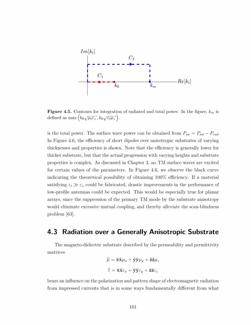
Figure 4.5. Contours for integration of radiated and total power. In the figure, km isdefined as max

(k0√µtεz , k0

√εtµz

).

is the total power. The surface wave power can be obtained from Psw = Ptot−Prad.In Figure 4.6, the efficiency of short dipoles over anisotropic substrates of varyingthicknesses and properties is shown. Note that the efficiency is generally lower forthicker substrate, but that the actual progression with varying heights and substrateproperties is complex. As discussed in Chapter 3, no TM surface waves are excitedfor certain values of the parameters. In Figure 4.6, we observe the black curveindicating the theoretical possibility of obtaining 100% efficiency. If a materialsatisfying εt � εz could be fabricated, drastic improvements in the performance oflow-profile antennas could be expected. This would be especially true for planararrays, since the suppression of the primary TM mode by the substrate anisotropywould eliminate excessive mutual coupling, and thereby alleviate the scan-blindnessproblem [63].

4.3 Radiation over a Generally Anisotropic SubstrateThe magneto-dielectric substrate described by the permeability and permittivity

matricesµ = xxµx + yyµy + zzµz

ε = xxεx + yyεy + zzεz

bears an influence on the polarization and pattern shape of electromagnetic radiationfrom impressed currents that is in some ways fundamentally different from what

101

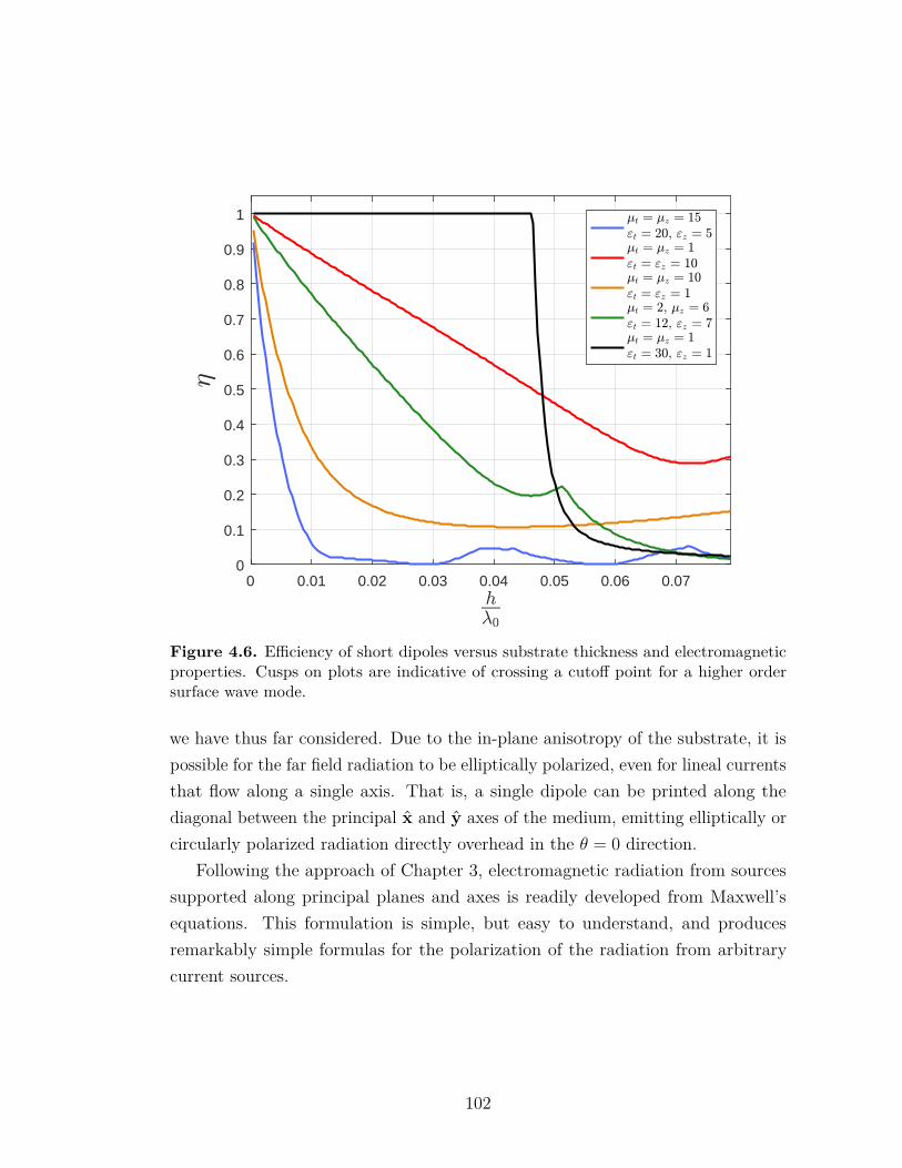
0 0.01 0.02 0.03 0.04 0.05 0.06 0.070

0.1

0.2

0.3

0.4

0.5

0.6

0.7

0.8

0.9

1

Figure 4.6. Efficiency of short dipoles versus substrate thickness and electromagneticproperties. Cusps on plots are indicative of crossing a cutoff point for a higher ordersurface wave mode.

we have thus far considered. Due to the in-plane anisotropy of the substrate, it ispossible for the far field radiation to be elliptically polarized, even for lineal currentsthat flow along a single axis. That is, a single dipole can be printed along thediagonal between the principal x and y axes of the medium, emitting elliptically orcircularly polarized radiation directly overhead in the θ = 0 direction.

Following the approach of Chapter 3, electromagnetic radiation from sourcessupported along principal planes and axes is readily developed from Maxwell’sequations. This formulation is simple, but easy to understand, and producesremarkably simple formulas for the polarization of the radiation from arbitrarycurrent sources.

102

4.3.1 Necessary Conditions for the Excitation of CircularlyPolarized Radiation Fields

The stationary phase formula for the far-field radiation due to an impressedcurrent distribution at z = 0 is (4.56), which we repeat below

E1(r) = jk0 cos θE1(kts , z = 0)e−jk0r

2πr

The radiation in the direction θ = 0 is obtained by evaluating E1(kts) for kxs =kys = 0. This can be thought of as the zero-frequency, or DC component of theplane wave spectrum. The general solution for the spectral fields, for kt = 0 takesthe form of a combination of TEM plane waves propagating along z. Within theanisotropic substrate, these waves were characterized in Chapter 3, Section 2.1.With kt = 0, the general solutions for the substrate and air region are

E1(kt = 0) = (xc1 + yc2) e−jk0z (4.100)

H1(kt = 0) =(

yc1

η0− x

c2

η0

)e−jk0z (4.101)

E2(kt = 0) = xc3 sin(k0√εxµy (z + h)

)+ yc4 sin

(k0√εyµx (z + h)

)(4.102)

H2(kt = 0) = yc3

η0

√εxµy

cos(k0√εxµy (z + h)

)− x

c4

η0

√εyµx

cos(k0√εyµx (z + h)

)(4.103)

where c1-c4 are unknown coefficients to be determined from the boundary conditions(4.6)-(4.7), with Js evaluated at kt = 0. Note that Js(kt = 0) has a meaningfulphysical interpretation,

Js(kt = 0) =+∞¨−∞

Js(r′) dx′ dy′ = jωp (4.104)

where p is the electric dipole moment of the current distribution [64, pg. 410].Evaluation of the unknown constants from the boundary conditions is a straight-

103

forward process. We find

E1(kt = 0) = −jη0

xxsin

(k0√εxµy h

)Dx

+ yysin

(k0√εyµx h

)Dy

· Js(kt = 0)e−jk0z

(4.105)where

Dx = j sin(k0√εxµy h

)+√εxµy

cos(k0√εxµy h

)(4.106)

Dy = j sin(k0√εyµx h

)+√εyµx

cos(k0√εyµx h

)(4.107)

Using (4.105) in (4.56) yields the desired result

E1(r) = k0η0

xxsin

(k0√εxµy h

)Dx

+ yysin

(k0√εyµx h

)Dy

· Js(kt = 0)e−jk0r

2πr(4.108)

Right hand circular polarization is achieved if Ey = −jEx. Suppose the radiatorwas a simple linear antenna directed along the vector a = 1

2(x + y). The currentdistribution is then of the form Js = af(kx, ky). Under these conditions, we seefrom (4.108) that right hand circular polarization requires

sin(k0√εyµx h

)Dy

= −jsin

(k0√εxµy h

)Dx

(4.109)

Provided εyµx 6= εxµy (4.109) has a solution for h, thus it is possible to obtaincircularly polarized radiation from a simple linear radiator with a single feed.

A related prototype has been reported in the literature [3], in which a crosseddipole consisting of two dipoles situated over different anisotropic magneto-dielectricmaterial samples is configured for circular polarization. Our theory shows that ifbetter control over the material properties was possible, that the antenna designcould be simplified to consist of a single dipole oriented at an angle with respect tothe principal axes of a single anisotropic magneto-dielectric material sample.

104

4.3.2 Principal Plane Radiation

The radiation from an arbitrary current source within the principal x− z andy − z planes can be obtained utilizing the technique introduced in the previoussection. Again, our starting point is the equation

E1(r) = jk0 cos θE1(kts , z = 0)e−jk0r

2πr

Within the x − z plane, we have y = 0. As a consequence, kys = 0. Thus, theradiated field within this principal plane is

E1(x, y = 0, z) = jk0 cos θE1(kts = xkxs , z = 0)e−jk0r

2πr (4.110)

In the y− z plane, kxs = 0, and the formula for the electric field is

E1(x = 0, y, z) = jk0 cos θE1(kts = ykys , z = 0)e−jk0r

2πr (4.111)

In view of (4.55),

E1(kts = xkxs , z = 0) = GE1(kts = xkxs , z = 0) · Js (4.112)

E1(kts = ykys , z = 0) = GE1(kts = ykys , z = 0) · Js (4.113)

Based on (4.112) and (4.113), we must determine GE1(kx, ky = 0, z = 0) andGE1(kx = 0, ky, z = 0). These quantities may be derived by following the procedureexplained in Section 4.2 exactly, step for step. The procedure from Section 4.2applies, even though the substrate has a more general anisotropy, because we haveconstrained our observations to principal planes. By the analysis of Chapter 3, theequations for TE and TM plane waves in principal planes are nearly identical tothose for TE and TM plane waves in the substrate with in-plane isotropy. The finalexpression (4.51) for an in-plane isotropic substrate can be immediately adaptedfor applicability to principal plane radiation. For instance, replacements such as µxor µy for µt will need to be made, depending on which principal plane, and whetherthe wave is TE or TM. The appropriate replacements may be determined from areview of Chapter 3. Additionally, kt is replaced with kx or ky depending on the

105

principal plane. A subtlety to notice is that kt for kx = 0 is equivalent to y sgn(ky),where sgn( ) is the sign function, equal to −1 for negative argument and +1 forpositive argument.

Introducing the notationx± = x sgn(kx)

y± = y sgn(ky)

Then the desired formulas are

GE1(kx, 0, 0) = −jη0k0

((x± − kx

kz1

z)x±kzckz1 sin(kzch)k2

0Txzm

+ yyµx sin(kzd

h)T xze

)(4.114)

GE1(0, ky, 0) = −jη0k0

((y± − ky

kz1

z)y±kzbkz1 sin(kzb

h)k2

0Tyzm

+ xxµy sin(kzah)

T yze

)(4.115)

wherekza =

√εxµyk2

0 −µyµzk2y (4.116)

kzb=√εyµxk2

0 −εyεzk2y (4.117)

kzc =√εxµyk2

0 −εxεzk2x (4.118)

kzd=√εyµxk2

0 −µxµzk2x (4.119)

andT xzm = εxkz1 cos(kzch) + jkzc sin(kzch) (4.120)

T xze = jµxkz1 sin(kzdh) + kzd

cos(kzdh) (4.121)

T yzm = εykz1 cos(kzbh) + jkzb

sin(kzbh) (4.122)

T yze = jµykz1 sin(kzah) + kza cos(kzah) (4.123)

In order to demonstrate the use of these formulas in the determination of theradiated fields from a prescribed current distribution, let us consider again thex-directed very short dipole antenna, for which Js = x`I0. Combining (4.110),(4.112), and (4.114), the radiated electric field in the x− z plane can be shown to

106

beE1(x, 0, z) = k0η0`I0θ(θ · x)kzcs

sin(kzcsh)

T xzms

e−jk0r

2πr (4.124)

Similarly, combining (4.111), (4.113), and (4.115), the radiated electric field in they− z plane is

E1(0, y, z) = k0η0`I0φ(φ · x)µyk0 cos θ sin(kzash)

T yzes

e−jk0r

2πr (4.125)

For a y directed short dipole, we instead obtain the principal plane patterns

E1(x, 0, z) = k0η0`I0φ(φ · y)µxk0 cos θ sin(kzds

h)T xzes

e−jk0r

2πr (4.126)

E1(0, y, z) = k0η0`I0θ(θ · y)kzbs

sin(kzbsh)

T yzms

e−jk0r

2πr (4.127)

Comparison of (4.124) to (4.127), and (4.125) to (4.126), reveals a unique featureresulting from in-plane anisotropy. Namely, rotating the source of the radiationfrom the x axis to the y axis does not result in the same radiation pattern rotatedby 90◦.

By the appropriate replacements of µt and εt with µx, εy or µy, εx, the detailedbehavior of the principal plane patterns matches that of the patterns shown inFigures 4.2 and 4.3.

107

Chapter 5 |Method of Moments Analysisof Microstrip Dipoles

In this chapter, the theory presented in previous chapters is utilized to developa method of moments algorithm for the analysis of center-fed printed microstripdipole antennas lying over a grounded anisotropic magneto-dielectric substrate.

The Green’s functions derived in Chapter 4 allow the electric field due toan arbitrary current source to be calculated at any location. By enforcing therequirement that the total electric field tangential to the surface of the dipole bezero, an integral equation for the unknown currents may be obtained. The methodof moments procedure is used to obtain approximate solutions to the integralequation.

The microstrip dipole is modeled with a delta-gap voltage source. The unknowncurrents are expressed in terms of a set of subdomain basis functions, and Galerkin’sprocedure is utilized, in which the testing functions are equal to the basis functions.The impedance matrix elements are evaluated using numerical integration in thespectral domain. Details on the implementation of the algorithm are given in thesubsequent sections of this Chapter. Results are given in the concluding section.

5.1 Spectral Formulation of the Electric-Field Inte-gral Equation

The microstrip dipole antenna of length L and width W , where L� W , canbe modeled effectively starting from the electric field integral equation (EFIE).

108

Let Ei(r) be the tangential electric field introduced by a source impressed on thesurface S of the antenna. This impressed source induces an electric surface currentJs(r) to flow on the dipole antenna, which, in turn, produces a scattered tangentialfield Es(r). The EFIE, for r ∈ {S}, is

Ei(r) = −Es(r) (5.1)

Using (4.80), Es(r) can be expressed in terms of Js(r). We have

Ei(r) = − 1(2π)2

+∞¨−∞

GE1 · Jse−jkt·r dkx dky (5.2)

where GE1 is evaluated at z = 0. Next, we express the unknown current distributionin a sum of subdomain basis functions. We assume the long dimension of the dipoleis x directed. Furthermore, we assume the current has no transverse y component,which is reasonable for a very thin microstrip dipole. The total number of basisfunctions used is N .

Js = xN∑n=1

Infn(x, y) (5.3)

In (5.3), In are the unknown amplitudes of the basis functions fn(x, y). Substitutionof (5.3) into (5.2) yields

Ei(r) = − 1(2π)2

N∑n=1

In

+∞¨−∞

GE1 · xfn(kx, ky)e−jkt·r dkx dky (5.4)

where fn(kx, ky) is the double Fourier transform of fn(x, y). In order to obtain Nequations in the N unknown coefficients In, we take the dot product of both sidesof (5.4) with xfm(x, y) and integrate over S.

¨

S

fmx · Ei(r) dS = − 1(2π)2

N∑n=1

In

¨

S

xfm ·

+∞¨−∞

GE1 · xfne−jkt·r dkx dky

dS

(5.5)

109

Then, we interchange the order of integration.

¨

S

fmx · Ei(r) dS = − 1(2π)2

N∑n=1

In

+∞¨−∞

¨

S

fme−jkt·r dS

(

x · GE1 · x)fn dkx dky

(5.6)We will assume that fm is a real function of x and y. In this case,

¨

S

fme−jkt·r dS =

¨

S

fmejkt·r dS

∗

= fm∗ (5.7)

where z∗ is the complex conjugate operation. Hence, (5.6) becomes

¨

S

fmx · Ei(r) dS = − 1(2π)2

N∑n=1

In

+∞¨−∞

(x · GE1 · x

)fm∗fn dkx dky (5.8)

For m = 1, 2, ..., N , we obtain from (5.8) N equations for the unknown currentamplitudes In. These N equations form a linear algebraic system,

[V]

=[Z]·[I]

(5.9)

where [I]

=[I1 I2 · · · IN

]T(5.10)[

V]

=[V1 V2 · · · VN

]T(5.11)

[Z]

=

Z11 Z12 · · · Z1N

Z21. . . ...

... . . . ...ZN1 · · · · · · ZNN

(5.12)

[Z]is commonly called the impedance matrix, and

[V]the voltage column. The

elements of the impedance matrix and voltage column are

Zmn = − 1(2π)2

+∞¨−∞

(x · GE1 · x

)fm∗fn dkx dky (5.13)

110

Vm =¨

S

fmx · Ei(r) dS (5.14)

From (4.51),

x · GE1 · x = −jη0

k2xkzakz1 sin(kzah)

k2t k0Tm

+µtk

2yk0 sin(kzb

h)k2t Te

(5.15)

In the next section, we discuss the specific choice of basis functions and theconvergence of the resulting integrals for the impedance matrix elements Zmn.

5.2 Basis Functions and Source ModelThe basis functions we employ are taken from [18, pp.353-359]. We set

fn(x, y) = 1W

tri(x

d− xn

)rect

(y

W

)(5.16)

whered = L

N + 1 (5.17)

xn = nd (5.18)

rect( ) is the rectangular function, defined as

rect(x) = U(x+ 1

2

)− U

(x− 1

2

)(5.19)

and U( ) is the unit step function. tri( ) is the triangular function, defined as

tri(x) = rect(x

2

) (1−|x|

)(5.20)

In Figure 5.1, a plot of the x-dependence of the basis functions along the dipolelength is shown for N = 3.

The double Fourier transform of the basis function is

fn(kx, ky) = dejkxxnsin

(kyW

2

)kyW

2

sin2(kxd2

)(kxd2

)2 (5.21)

111

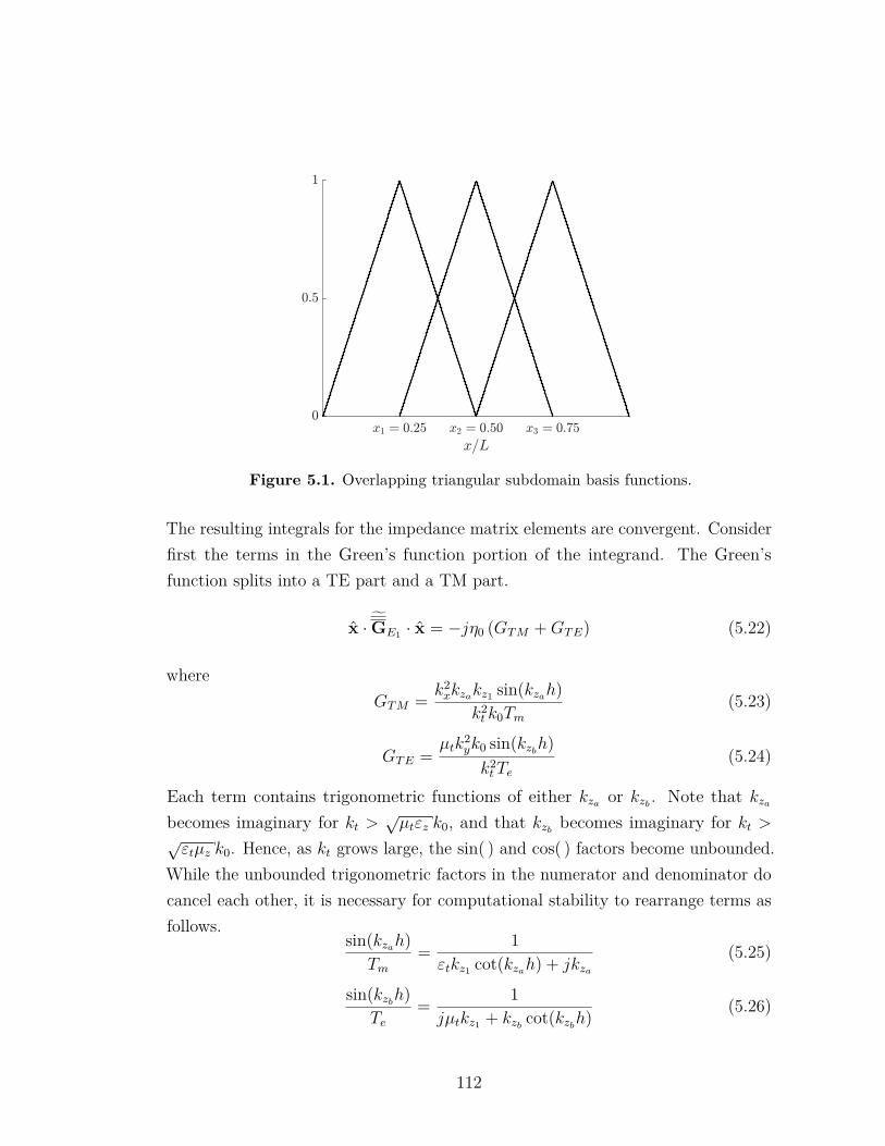
Figure 5.1. Overlapping triangular subdomain basis functions.

The resulting integrals for the impedance matrix elements are convergent. Considerfirst the terms in the Green’s function portion of the integrand. The Green’sfunction splits into a TE part and a TM part.

x · GE1 · x = −jη0 (GTM +GTE) (5.22)

whereGTM = k2

xkzakz1 sin(kzah)k2t k0Tm

(5.23)

GTE =µtk

2yk0 sin(kzb

h)k2t Te

(5.24)

Each term contains trigonometric functions of either kza or kzb. Note that kza

becomes imaginary for kt >√µtεz k0, and that kzb

becomes imaginary for kt >√εtµz k0. Hence, as kt grows large, the sin( ) and cos( ) factors become unbounded.

While the unbounded trigonometric factors in the numerator and denominator docancel each other, it is necessary for computational stability to rearrange terms asfollows.

sin(kzah)Tm

= 1εtkz1 cot(kzah) + jkza

(5.25)

sin(kzbh)

Te= 1jµtkz1 + kzb

cot(kzbh) (5.26)

112

This is a superior arrangement of terms, since cot(kzah) and cot(kzbh) both rapidly

approach an asymptotic value of j as kt →∞. We observe that the terms in (5.25)and (5.26) behave asymptotically like k−1

t . From this fact, we see that GTM behaveslike kt and GTE behaves like k−1

t .The linearly growing nature of GTM implies that the integrals for the impedance

matrix elements would not be convergent for an arbitrary choice of basis andtesting functions. In fact, if we had attempted to utilize rectangular basis functionsand delta testing functions, we would have obtained divergent integrals for theimpedance matrix elements.1 With our choice of basis and testing functions, alongthe ky axis the complete integrand for Zmn behaves like k−3

y . Similarly, along thekx axis, the integrand behaves asymptotically like k−3

x .2 We observe that Zmnwould be impossible to evaluate for the limiting case of a filamentary dipole withinfinitesimal width W . In this case, the integrals would behave like k−1

y along theky axis, integrating asymptotically to ln(ky) which is unbounded as ky →∞.

The source model for the microstrip dipole is the delta gap generator. Lettingnc = N+1

2 , we haveEi(r) = xV0δ(x− xnc) rect

(y

W

)(5.27)

The resulting voltage column elements are

Vm =¨

S

fmx · Ei(r) dS =

V0 m = N+1

2

0 m 6= N+12

(5.28)

5.3 Numerical IntegrationThe integration interval ranges from ±∞ in both kx and ky. By taking advantage

of existing symmetries in the functions composing the integrand, this can be reducedto an integration over the first quadrant in the kx-ky plane [18]. First, we denote

1Divergent integrals obtained through a poor choice of basis and testing functions can betraced back to the interchangement of the order of integrations involved in the derivation of(5.13). The step where integrals over S and kx and ky are interchanged is rigorous only if theresulting formulas are convergent.

2The integrand would not converge along the kx axis if the x-dependence of the basis functionwas chosen to be the rectangular function instead of the triangular function. In this case, theintegrand would behave like k−1

x along the kx axis.

113

the integrand

K(kx, ky) = −jη0 (GTM +GTE) d2ejkx(xn−xm) sin2(kyW

2

)(kyW

2

)2

sin4(kxd2

)(kxd2

)4 (5.29)

In terms of K(kx, ky), the impedance matrix elements are

Zmn = − 1(2π)2

+∞¨−∞

K(kx, ky) dkx dky (5.30)

Since K(kx,−ky) = K(kx, ky), (5.30) is equivalent to

Zmn = − 2(2π)2

+∞ˆ

0

+∞ˆ−∞

K(kx, ky) dkx dky (5.31)

Next, we may express the integrand in the form

K(kx, ky) = ejkx(xn−xm)F (kx, ky) (5.32)

where

F (kx, ky) = −jη0 (GTM +GTE) d2 sin2(kyW

2

)(kyW

2

)2

sin4(kxd2

)(kxd2

)4 (5.33)

Using Euler’s identity,

ejkx(xn−xm) = cos(kx(xn − xm)

)+ j sin

(kx(xn − xm)

)(5.34)

Then, we observe

cos(−kx(xn − xm)

)F (−kx, ky) = cos

(kx(xn − xm)

)F (kx, ky) (5.35)

and

sin(−kx(xn − xm)

)F (−kx, ky) = − sin

(kx(xn − xm)

)F (kx, ky) (5.36)

Thus, the integrand splits into two parts, one is even in the integration variable kx,and the other part is odd. The integration of an odd function of kx from −∞ to

114

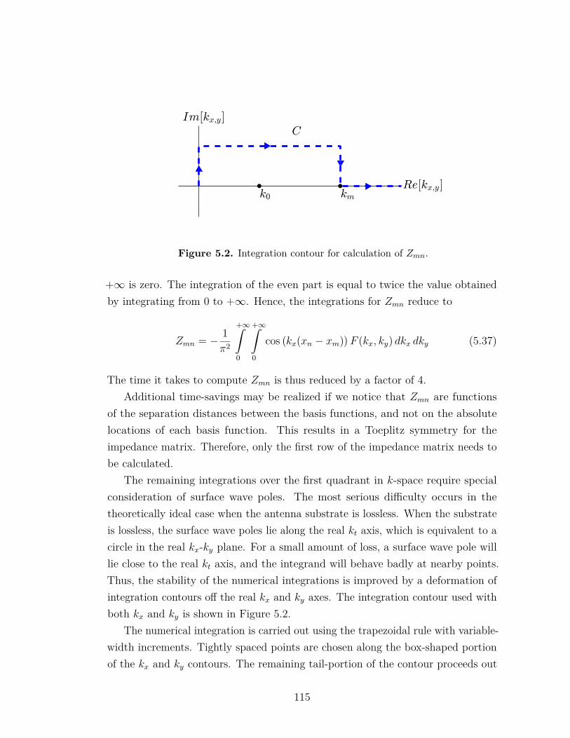
Figure 5.2. Integration contour for calculation of Zmn.

+∞ is zero. The integration of the even part is equal to twice the value obtainedby integrating from 0 to +∞. Hence, the integrations for Zmn reduce to

Zmn = − 1π2

+∞ˆ

0

+∞ˆ

0

cos(kx(xn − xm)

)F (kx, ky) dkx dky (5.37)

The time it takes to compute Zmn is thus reduced by a factor of 4.Additional time-savings may be realized if we notice that Zmn are functions

of the separation distances between the basis functions, and not on the absolutelocations of each basis function. This results in a Toeplitz symmetry for theimpedance matrix. Therefore, only the first row of the impedance matrix needs tobe calculated.

The remaining integrations over the first quadrant in k-space require specialconsideration of surface wave poles. The most serious difficulty occurs in thetheoretically ideal case when the antenna substrate is lossless. When the substrateis lossless, the surface wave poles lie along the real kt axis, which is equivalent to acircle in the real kx-ky plane. For a small amount of loss, a surface wave pole willlie close to the real kt axis, and the integrand will behave badly at nearby points.Thus, the stability of the numerical integrations is improved by a deformation ofintegration contours off the real kx and ky axes. The integration contour used withboth kx and ky is shown in Figure 5.2.

The numerical integration is carried out using the trapezoidal rule with variable-width increments. Tightly spaced points are chosen along the box-shaped portionof the kx and ky contours. The remaining tail-portion of the contour proceeds out

115

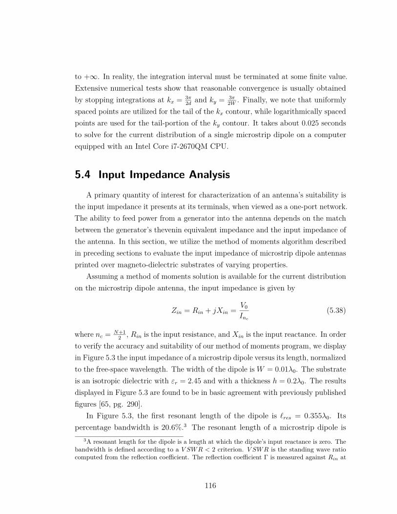
to +∞. In reality, the integration interval must be terminated at some finite value.Extensive numerical tests show that reasonable convergence is usually obtainedby stopping integrations at kx = 3π

2d and ky = 3π2W . Finally, we note that uniformly

spaced points are utilized for the tail of the kx contour, while logarithmically spacedpoints are used for the tail-portion of the ky contour. It takes about 0.025 secondsto solve for the current distribution of a single microstrip dipole on a computerequipped with an Intel Core i7-2670QM CPU.

5.4 Input Impedance AnalysisA primary quantity of interest for characterization of an antenna’s suitability is

the input impedance it presents at its terminals, when viewed as a one-port network.The ability to feed power from a generator into the antenna depends on the matchbetween the generator’s thevenin equivalent impedance and the input impedance ofthe antenna. In this section, we utilize the method of moments algorithm describedin preceding sections to evaluate the input impedance of microstrip dipole antennasprinted over magneto-dielectric substrates of varying properties.

Assuming a method of moments solution is available for the current distributionon the microstrip dipole antenna, the input impedance is given by

Zin = Rin + jXin = V0

Inc

(5.38)

where nc = N+12 , Rin is the input resistance, and Xin is the input reactance. In order

to verify the accuracy and suitability of our method of moments program, we displayin Figure 5.3 the input impedance of a microstrip dipole versus its length, normalizedto the free-space wavelength. The width of the dipole is W = 0.01λ0. The substrateis an isotropic dielectric with εr = 2.45 and with a thickness h = 0.2λ0. The resultsdisplayed in Figure 5.3 are found to be in basic agreement with previously publishedfigures [65, pg. 290].

In Figure 5.3, the first resonant length of the dipole is `res = 0.355λ0. Itspercentage bandwidth is 20.6%.3 The resonant length of a microstrip dipole is

3A resonant length for the dipole is a length at which the dipole’s input reactance is zero. Thebandwidth is defined according to a V SWR < 2 criterion. V SWR is the standing wave ratiocomputed from the reflection coefficient. The reflection coefficient Γ is measured against Rin at

116

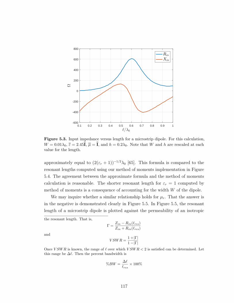
0.1 0.2 0.3 0.4 0.5 0.6 0.7 0.8 0.9 1-600

-400

-200

0

200

400

600

800

Figure 5.3. Input impedance versus length for a microstrip dipole. For this calculation,W = 0.01λ0, ε = 2.45I, µ = I, and h = 0.2λ0. Note that W and h are rescaled at eachvalue for the length.

approximately equal to (2(εr + 1))−1/2λ0 [65]. This formula is compared to theresonant lengths computed using our method of moments implementation in Figure5.4. The agreement between the approximate formula and the method of momentscalculation is reasonable. The shorter resonant length for εr = 1 computed bymethod of moments is a consequence of accounting for the width W of the dipole.

We may inquire whether a similar relationship holds for µr. That the answer isin the negative is demonstrated clearly in Figure 5.5. In Figure 5.5, the resonantlength of a microstrip dipole is plotted against the permeability of an isotropic

the resonant length. That is,Γ = Zin −Rin(`res)

Zin +Rin(`res)and

V SWR = 1 +|Γ|1−|Γ|

Once V SWR is known, the range of ` over which V SWR < 2 is satisfied can be determined. Letthis range be ∆`. Then the percent bandwidth is

%BW = ∆``res× 100%

117

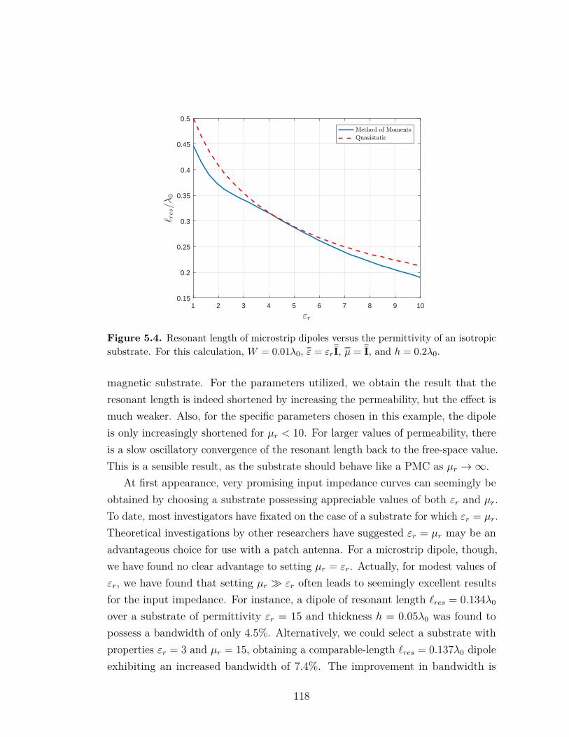
1 2 3 4 5 6 7 8 9 100.15

0.2

0.25

0.3

0.35

0.4

0.45

0.5

Figure 5.4. Resonant length of microstrip dipoles versus the permittivity of an isotropicsubstrate. For this calculation, W = 0.01λ0, ε = εrI, µ = I, and h = 0.2λ0.

magnetic substrate. For the parameters utilized, we obtain the result that theresonant length is indeed shortened by increasing the permeability, but the effect ismuch weaker. Also, for the specific parameters chosen in this example, the dipoleis only increasingly shortened for µr < 10. For larger values of permeability, thereis a slow oscillatory convergence of the resonant length back to the free-space value.This is a sensible result, as the substrate should behave like a PMC as µr →∞.

At first appearance, very promising input impedance curves can seemingly beobtained by choosing a substrate possessing appreciable values of both εr and µr.To date, most investigators have fixated on the case of a substrate for which εr = µr.Theoretical investigations by other researchers have suggested εr = µr may be anadvantageous choice for use with a patch antenna. For a microstrip dipole, though,we have found no clear advantage to setting µr = εr. Actually, for modest values ofεr, we have found that setting µr � εr often leads to seemingly excellent resultsfor the input impedance. For instance, a dipole of resonant length `res = 0.134λ0

over a substrate of permittivity εr = 15 and thickness h = 0.05λ0 was found topossess a bandwidth of only 4.5%. Alternatively, we could select a substrate withproperties εr = 3 and µr = 15, obtaining a comparable-length `res = 0.137λ0 dipoleexhibiting an increased bandwidth of 7.4%. The improvement in bandwidth is

118

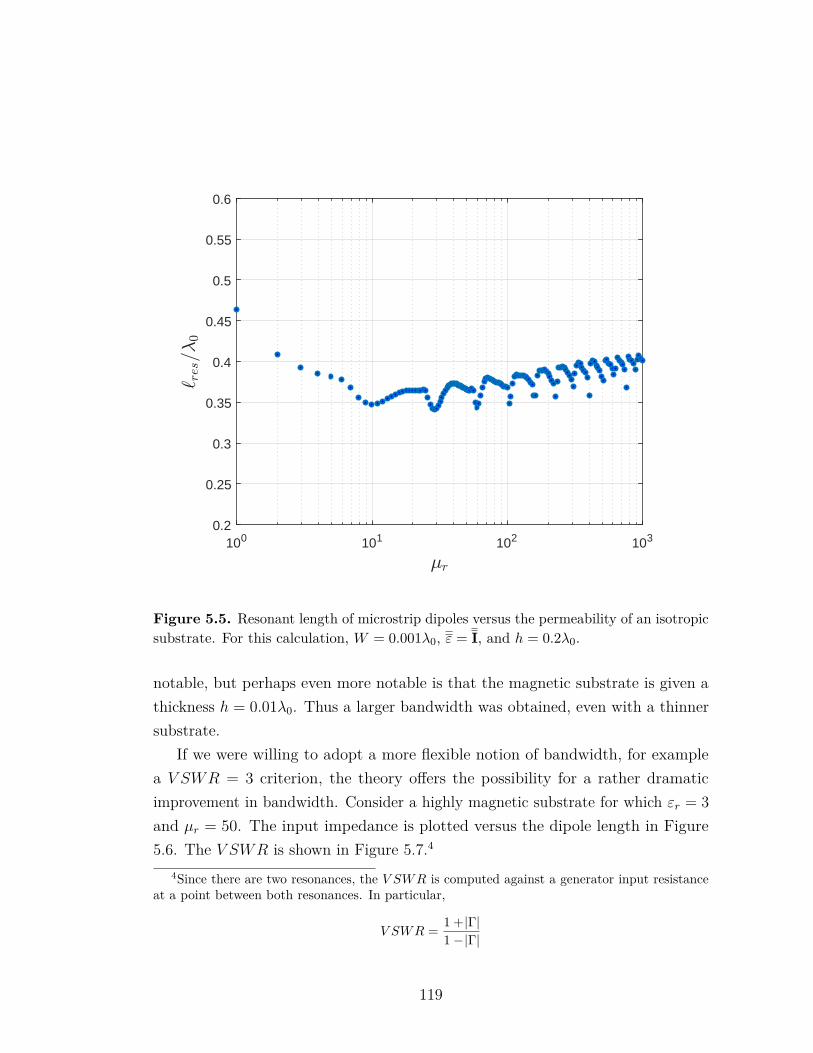
100 101 102 1030.2

0.25

0.3

0.35

0.4

0.45

0.5

0.55

0.6

Figure 5.5. Resonant length of microstrip dipoles versus the permeability of an isotropicsubstrate. For this calculation, W = 0.001λ0, ε = I, and h = 0.2λ0.

notable, but perhaps even more notable is that the magnetic substrate is given athickness h = 0.01λ0. Thus a larger bandwidth was obtained, even with a thinnersubstrate.

If we were willing to adopt a more flexible notion of bandwidth, for examplea V SWR = 3 criterion, the theory offers the possibility for a rather dramaticimprovement in bandwidth. Consider a highly magnetic substrate for which εr = 3and µr = 50. The input impedance is plotted versus the dipole length in Figure5.6. The V SWR is shown in Figure 5.7.4

4Since there are two resonances, the V SWR is computed against a generator input resistanceat a point between both resonances. In particular,

V SWR = 1 +|Γ|1−|Γ|

119

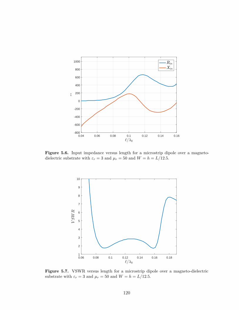
0.04 0.06 0.08 0.1 0.12 0.14 0.16-800

-600

-400

-200

0

200

400

600

800

1000

Figure 5.6. Input impedance versus length for a microstrip dipole over a magneto-dielectric substrate with εr = 3 and µr = 50 and W = h = L/12.5.

0.06 0.08 0.1 0.12 0.14 0.16 0.181

2

3

4

5

6

7

8

9

10

Figure 5.7. VSWR versus length for a microstrip dipole over a magneto-dielectricsubstrate with εr = 3 and µr = 50 and W = h = L/12.5.

120

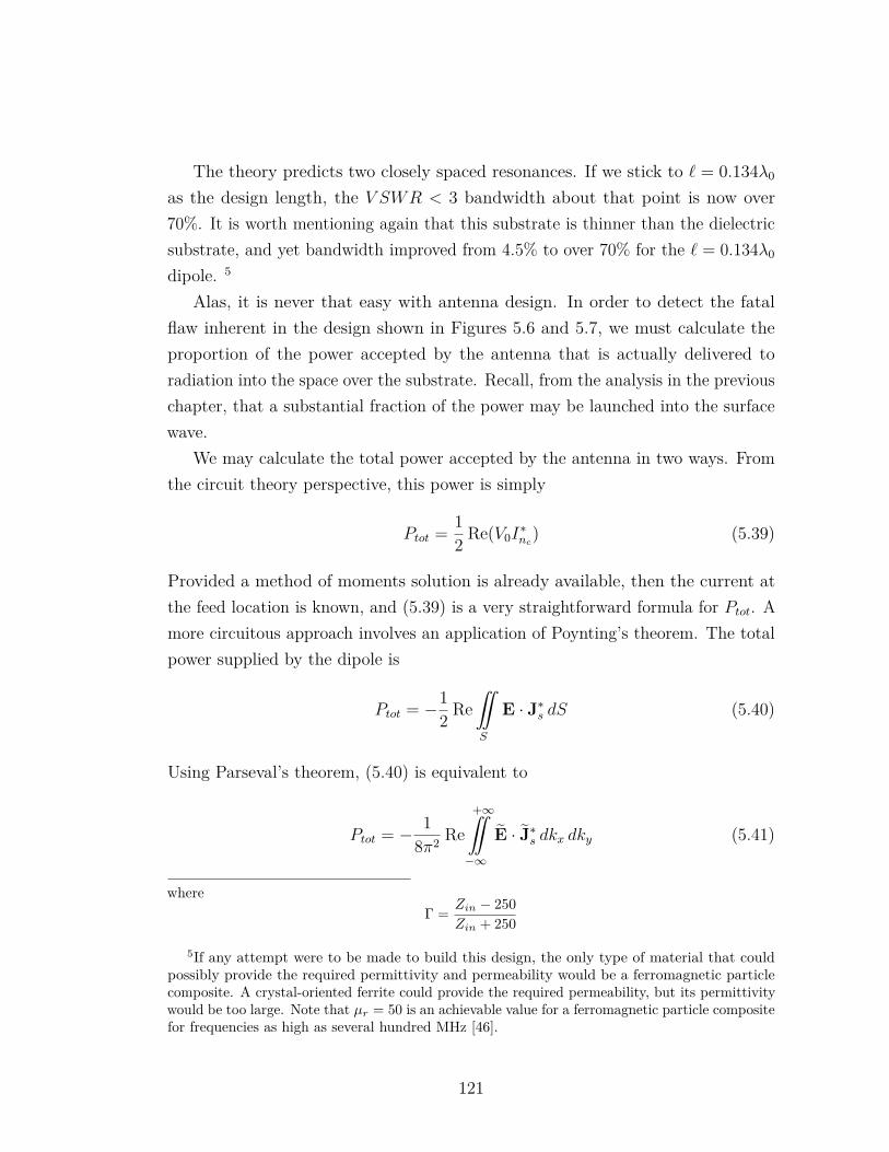
The theory predicts two closely spaced resonances. If we stick to ` = 0.134λ0

as the design length, the V SWR < 3 bandwidth about that point is now over70%. It is worth mentioning again that this substrate is thinner than the dielectricsubstrate, and yet bandwidth improved from 4.5% to over 70% for the ` = 0.134λ0

dipole. 5

Alas, it is never that easy with antenna design. In order to detect the fatalflaw inherent in the design shown in Figures 5.6 and 5.7, we must calculate theproportion of the power accepted by the antenna that is actually delivered toradiation into the space over the substrate. Recall, from the analysis in the previouschapter, that a substantial fraction of the power may be launched into the surfacewave.

We may calculate the total power accepted by the antenna in two ways. Fromthe circuit theory perspective, this power is simply

Ptot = 12 Re(V0I

∗nc

) (5.39)

Provided a method of moments solution is already available, then the current atthe feed location is known, and (5.39) is a very straightforward formula for Ptot. Amore circuitous approach involves an application of Poynting’s theorem. The totalpower supplied by the dipole is

Ptot = −12 Re

¨

S

E · J∗s dS (5.40)

Using Parseval’s theorem, (5.40) is equivalent to

Ptot = − 18π2 Re

+∞¨−∞

E · J∗s dkx dky (5.41)

whereΓ = Zin − 250

Zin + 250

5If any attempt were to be made to build this design, the only type of material that couldpossibly provide the required permittivity and permeability would be a ferromagnetic particlecomposite. A crystal-oriented ferrite could provide the required permeability, but its permittivitywould be too large. Note that µr = 50 is an achievable value for a ferromagnetic particle compositefor frequencies as high as several hundred MHz [46].

121

In terms of the Green’s function, (5.41) is

Ptot = − 18π2 Re

¨

S

J∗s · GE1 · Js dS (5.42)

Upon substitution of (5.3) into (5.42) we obtain

Ptot = − 18π2 Re

N∑m=1

N∑n=1

I∗mIn

+∞¨−∞

(x · GE1 · x

)fm∗fn dkx dky (5.43)

According to (5.13), the infinite integrals appearing in the summand are theimpedance matrix elements Zmn. We have

Ptot = 12 Re

N∑m=1

N∑n=1

I∗mInZmn (5.44)

In terms of the impedance matrix and current column, (5.44) is

Ptot = 12 Re

([I]H·[Z]·[I])

(5.45)

where[I]H

is the Hermitian, or complex conjugate transpose of[I]. Numerical

calculation of Ptot using (5.45) always agrees with the simple circuit theory calcula-tion indicated in (5.39). Equation (5.45) also suggests a formula for the radiationfield portion of the total power. Recall that the power integrated in k-space up tok0 is the radiated power, since for kt > k0, kz1 = −jα, and no propagation in the+z direction occurs. Thus, the formula for the radiated power, from (5.45), is

Prad = 12 Re

([I]H·[Rrad

]·[I])

(5.46)

where[Rrad

]is the square matrix whose entries Rmn are

Rmn = − 1(2π)2

k0¨

0

(x · GE1 · x

)fm∗fn dkx dky (5.47)

122

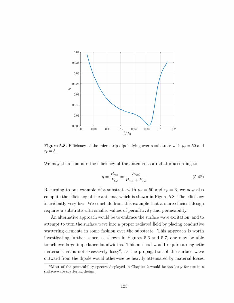
0.06 0.08 0.1 0.12 0.14 0.16 0.18 0.20.005

0.01

0.015

0.02

0.025

0.03

0.035

0.04

Figure 5.8. Efficiency of the microstrip dipole lying over a substrate with µr = 50 andεr = 3.

We may then compute the efficiency of the antenna as a radiator according to

η = PradPtot

= PradPrad + Psw

(5.48)

Returning to our example of a substrate with µr = 50 and εr = 3, we now alsocompute the efficiency of the antenna, which is shown in Figure 5.8. The efficiencyis evidently very low. We conclude from this example that a more efficient designrequires a substrate with smaller values of permittivity and permeability.

An alternative approach would be to embrace the surface wave excitation, and toattempt to turn the surface wave into a proper radiated field by placing conductivescattering elements in some fashion over the substrate. This approach is worthinvestigating further, since, as shown in Figures 5.6 and 5.7, one may be ableto achieve large impedance bandwidths. This method would require a magneticmaterial that is not excessively lossy6, as the propagation of the surface waveoutward from the dipole would otherwise be heavily attenuated by material losses.

6Most of the permeability spectra displayed in Chapter 2 would be too lossy for use in asurface-wave-scattering design.

123

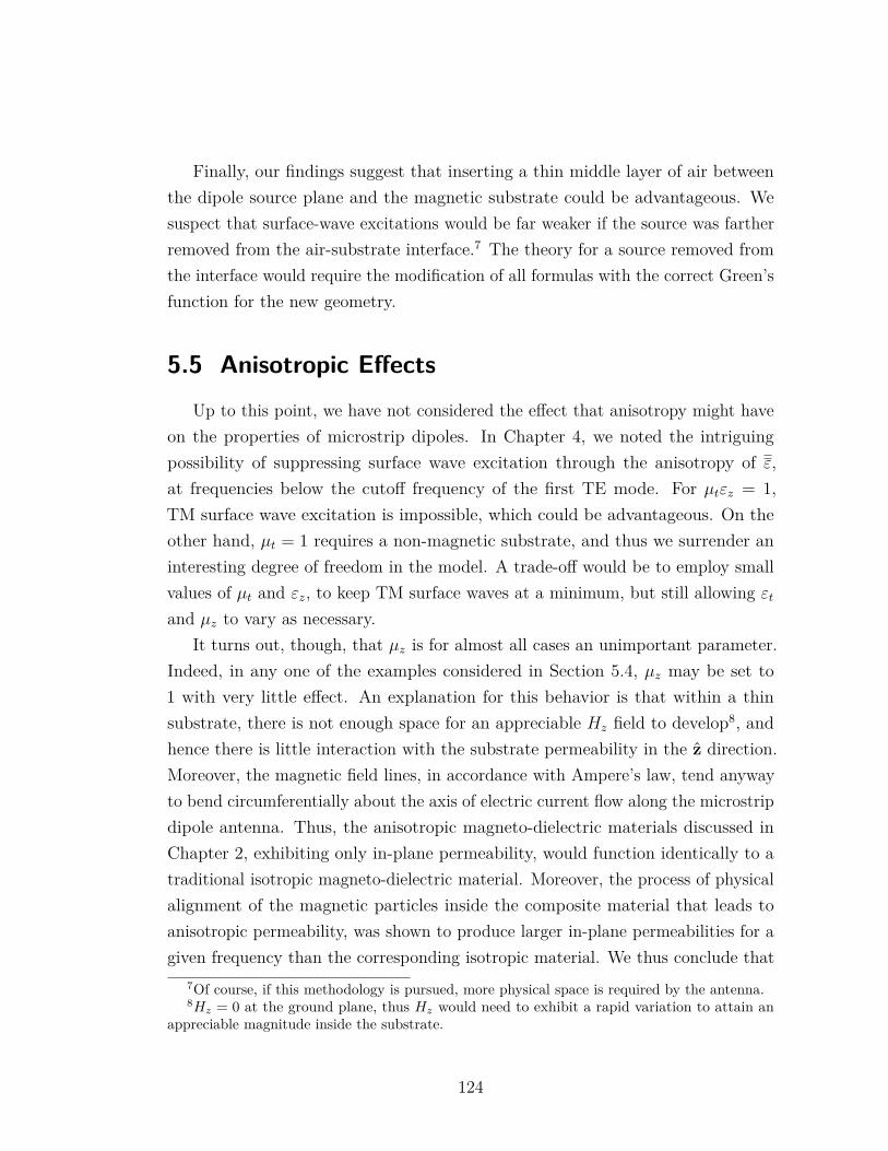
Finally, our findings suggest that inserting a thin middle layer of air betweenthe dipole source plane and the magnetic substrate could be advantageous. Wesuspect that surface-wave excitations would be far weaker if the source was fartherremoved from the air-substrate interface.7 The theory for a source removed fromthe interface would require the modification of all formulas with the correct Green’sfunction for the new geometry.

5.5 Anisotropic EffectsUp to this point, we have not considered the effect that anisotropy might have

on the properties of microstrip dipoles. In Chapter 4, we noted the intriguingpossibility of suppressing surface wave excitation through the anisotropy of ε,at frequencies below the cutoff frequency of the first TE mode. For µtεz = 1,TM surface wave excitation is impossible, which could be advantageous. On theother hand, µt = 1 requires a non-magnetic substrate, and thus we surrender aninteresting degree of freedom in the model. A trade-off would be to employ smallvalues of µt and εz, to keep TM surface waves at a minimum, but still allowing εtand µz to vary as necessary.

It turns out, though, that µz is for almost all cases an unimportant parameter.Indeed, in any one of the examples considered in Section 5.4, µz may be set to1 with very little effect. An explanation for this behavior is that within a thinsubstrate, there is not enough space for an appreciable Hz field to develop8, andhence there is little interaction with the substrate permeability in the z direction.Moreover, the magnetic field lines, in accordance with Ampere’s law, tend anywayto bend circumferentially about the axis of electric current flow along the microstripdipole antenna. Thus, the anisotropic magneto-dielectric materials discussed inChapter 2, exhibiting only in-plane permeability, would function identically to atraditional isotropic magneto-dielectric material. Moreover, the process of physicalalignment of the magnetic particles inside the composite material that leads toanisotropic permeability, was shown to produce larger in-plane permeabilities for agiven frequency than the corresponding isotropic material. We thus conclude that

7Of course, if this methodology is pursued, more physical space is required by the antenna.8Hz = 0 at the ground plane, thus Hz would need to exhibit a rapid variation to attain an

appreciable magnitude inside the substrate.

124

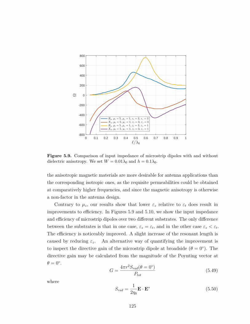
0 0.1 0.2 0.3 0.4 0.5 0.6 0.7 0.8 0.9 1-800

-600

-400

-200

0

200

400

600

800

Figure 5.9. Comparison of input impedance of microstrip dipoles with and withoutdielectric anisotropy. We set W = 0.01λ0 and h = 0.1λ0.

the anisotropic magnetic materials are more desirable for antenna applications thanthe corresponding isotropic ones, as the requisite permeabilities could be obtainedat comparatively higher frequencies, and since the magnetic anisotropy is otherwisea non-factor in the antenna design.

Contrary to µz, our results show that lower εz relative to εt does result inimprovements to efficiency. In Figures 5.9 and 5.10, we show the input impedanceand efficiency of microstrip dipoles over two different substrates. The only differencebetween the substrates is that in one case, εz = εt, and in the other case εz < εt.The efficiency is noticeably improved. A slight increase of the resonant length iscaused by reducing εz. An alternative way of quantifying the improvement isto inspect the directive gain of the microstrip dipole at broadside (θ = 0◦). Thedirective gain may be calculated from the magnitude of the Poynting vector atθ = 0◦.

G = 4πr2Srad(θ = 0◦)Ptot

(5.49)

whereSrad = 1

2η0E · E∗ (5.50)

125

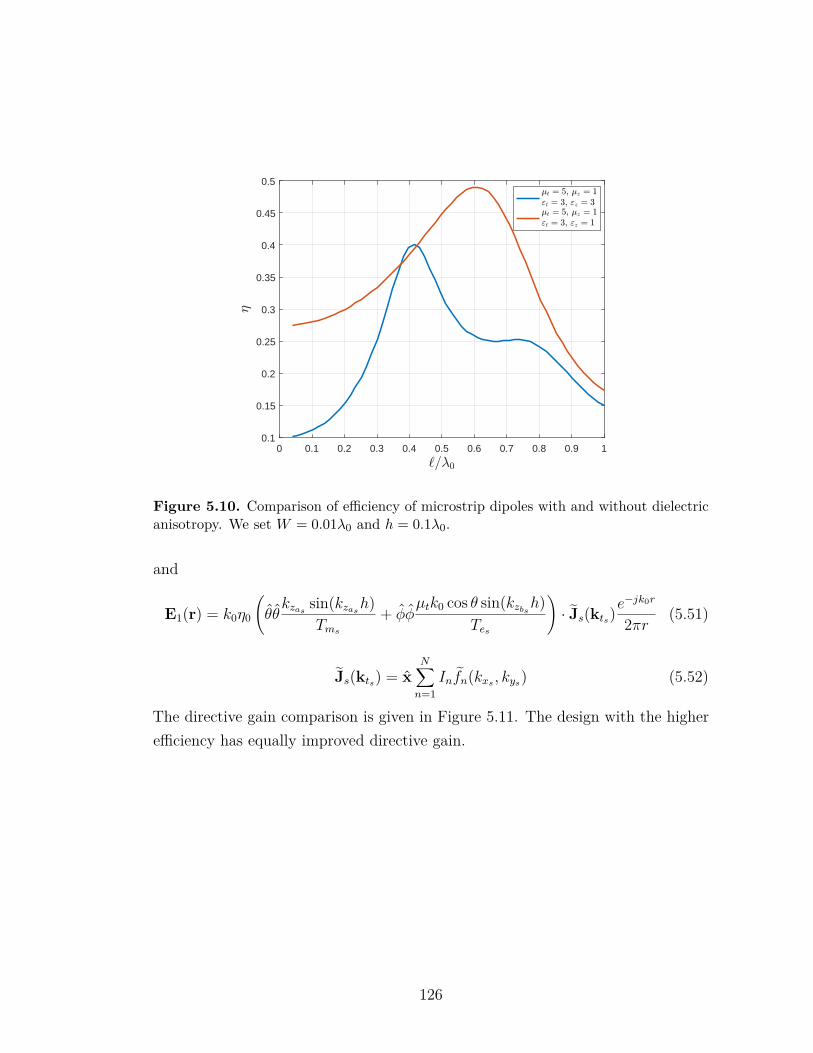
0 0.1 0.2 0.3 0.4 0.5 0.6 0.7 0.8 0.9 10.1

0.15

0.2

0.25

0.3

0.35

0.4

0.45

0.5

Figure 5.10. Comparison of efficiency of microstrip dipoles with and without dielectricanisotropy. We set W = 0.01λ0 and h = 0.1λ0.

and

E1(r) = k0η0

(θθkzas

sin(kzash)

Tms

+ φφµtk0 cos θ sin(kzbs

h)Tes

)· Js(kts)e

−jk0r

2πr (5.51)

Js(kts) = xN∑n=1

Infn(kxs , kys) (5.52)

The directive gain comparison is given in Figure 5.11. The design with the higherefficiency has equally improved directive gain.

126

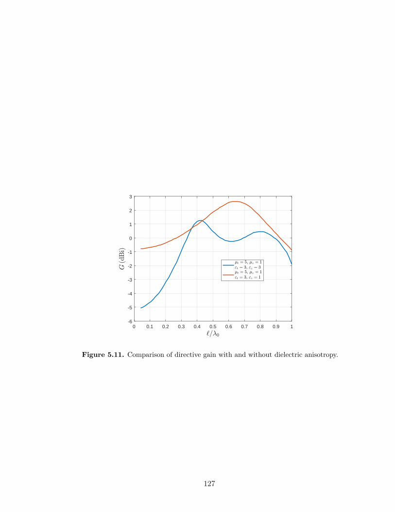
0 0.1 0.2 0.3 0.4 0.5 0.6 0.7 0.8 0.9 1-6

-5

-4

-3

-2

-1

0

1

2

3

Figure 5.11. Comparison of directive gain with and without dielectric anisotropy.

127

Chapter 6 |Conlusions and Future Work

Our method of moments analysis indicates that planar microstrip dipolesconstructed over magneto-dielectric substrates have inherently broader bandwidththan a dipole of the equivalent resonant length over a dielectric substrate. Moreover,the larger bandwidth may be achieved with a thinner substrate. To an extent, thiscan be explained by realizing that for a microstrip dipole, that the permeabilitydoes not influence the resonant length nearly as strongly as an equivalent value ofpermittivity. This behavior is not analogous to that of a rectangular patch. Forthe patch, we expect permeability and permittivity to influence resonant lengthequivalently. Again, this is not the case for a microstrip dipole. In fact, as µr →∞,the substrate begins to appear to the dipole as a PMC, and the resonant lengthapproaches its free-space value, which is close to λ0/2, depending to a small degreeon the width of the dipole.

Our analysis demonstrates that magneto-dielectric substrates are better attrapping waves in the form of propagating surface waves. We observe that antennadesigns made with strongly magnetic substrates often possess seemingly excellentimpedance bandwidth, but that the bandwidth is attributable to the excitation ofsurface waves. Radiation efficiency is therefore usually lower in a magneto-dielectricsubstrate, than in a dielectric substrate of an equivalent electrical thickness. Usingsubstrates of a small permeability, reasonable trade-offs between efficiency andbandwidth are attainable.

In theory, if εz could be minimized, then the efficiency problem could bealleviated. In fact, the theory shows that if µt = εz = 1, then no TM surface wavesare supported, and correspondingly higher efficiencies may be obtained. Our resultsshow that the resonant length is somewhat larger for a substrate with εz < εt, than

128

for the substrate of same εt where εz = εt. However, the resonant length does notrevert to the free space value, indicating that an appreciable tangential electric fieldexists in the substrate under the dipole, enabling interaction with the tangentialpermittivity εt.1

Lastly, calculations show for a thin substrate that µz is unimportant. Hence,when a larger permeability is desired, materials for which µz = 1 and µt � 1 maybe used without any negative consequence. For certain anisotropic materials, theSnoek product of permeability and resonance frequency is larger than the associatedisotropic material. As discussed in Chapter 2, such materials include the crystal-oriented ferrites, ferromagnetic laminates, and composites made with orientedferromagnetic flakes. On this basis, we conclude that anisotropic magneto-dielectricmaterials are better suited for low-profile planar antenna development. Thisconclusion only follows under the presumption that specified values of directionalpermeability and permittivity may be attained from a designed magnetic material.In Chapter 2, we summarized the current state of knowledge concerning thepermeability tensor for structured ferromagnetic materials. Crystalline anisotropyand demagnetization fields lead to anisotropic permeability for single domainmagnetic particles. Depending on the shape of the particle, and the directionof its crystal axes, this anisotropy can manifest in various ways. For example,a flattened oblate spheroidal particle may exhibit significant permeability alongjust the in-plane hard axis. Similarly, thin ferromagnetic films are magneticallyactive only along the in-plane hard axis. Ferrite fibers, possessing a crystal easyaxis along its long dimension, will have a significant permeability within the planeperpendicular to the easy axis, and a permeability of 1 along the easy axis. Thedetailed interaction between domains in large multi-domain ferrite fibers was derivedin Chapter 2, showing that while domain interactions do eliminate the naturallygyrotropic properties of the domains, the interactions do not eliminate all forms ofmacroscopically observable anisotropy in single crystals. For composites, a magneticfield may be applied to the material before it has hardened, causing an alignmentof particles which can be frozen in place as the material solidifies, thus enablinga macroscopically anisotropic material sample to be obtained. By controlling thedegree of alignment of the particles, or else by incorporating multiple varieties of

1The existence of an appreciable tangential electric field in the substrate indicates the insuffi-ciency of a traditional cavity model for the fields between the conducting dipole element and theconducting ground plane.

129

particles or microscopic materials, it seems plausible that the permeability alongvarious directions could be selected.

We can suggest a number of generalizations that could be made to the modeldeveloped in this Dissertation. The most important generalization, on the basis ofour calculations showing substantial surface wave excitation, would be to allow themodel to place a layer of free space between the microstrip dipole and the groundedmagneto-dielectric substrate. The addition of a middle layer would lead to antennadesigns requiring more physical space, but such a step appears to be necessaryto avoid a majority of the power accepted by the antenna from being deliveredinto the substrate. The method of moments algorithm detailed in this chaptercan be readily extended to handle sources removed from the substrate interfaceby evaluating the impedance matrix elements with the appropriately generalizedGreen’s function. Chapter 4 should be consulted for the needed methodology toobtain the appropriate Green’s function. A second, important generalization wouldbe to allow for material losses to be incorporated. The addition of losses wouldperturb the formulas for the cutoff frequencies, and the inequalities governing thelocations of the surface wave poles. Furthermore, some minor modifications to thecalculation of the loci for the integration contours for evaluating the impedancematrix elements are needed.

In Chapter 4, we showed that circularly polarized radiation can be obtainedusing a single-feed linear antenna by exploiting in-plane anisotropy of a magneto-dielectric substrate. Provided εxµy 6= εyµx, a substrate thickness can always bechosen to achieve circular polarization. This conclusion was reached irrespective ofthe exact details of the current distribution on the linear antenna. Thus, such adesign can be achieved using a microstrip dipole aligned at an angle with respectto the in-plane principal axes of the magneto-dielectric substrate. A methodof moments algorithm that can handle in-plane anisotropy, where εx 6= εy andµx 6= µy, is required for a detailed performance analysis. Along these lines, somework has been done in this Dissertation to develop an understanding of the wavepropagation behavior in such substrates. For instance, we have shown that TEMwaves are supported for wave propagation along a principal axis, and that TEand TM wave propagation is supported for wave propagation within a principalplane. For the TEM wave, the wave experiences an effective isotropic mediumwith an isotropic permittivity equal to the directional permittivity along the axis

130

that is parallel to the electric field, and an isotropic permeability equal to thedirectional permeabilitiy along the axis parallel to the magnetic field. A similarrelationship was uncovered for the TE and TM waves. Unlike isotropic media, theTE and TM waves carry power in a direction that is not parallel to the axis of phasepropagation. Interestingly, for other propagation directions, hybrid, and possiblycomplex waves propagate, exhibiting backward wave behavior. Moreover, thereexist mode pairs, closely related to evanescent waves in cutoff, whose propagationconstants are complex conjugates of each other, and for which power orthogonalityis not maintained. Of additional interest would be a theoretical investigation of theform taken by outwardly propagating cylindrical surface waves, since our analysisshows that the expressions for the cutoff frequencies depends on the local directionof propagation. Such a cylindrical wave must therefore be spatially dispersive. Thedetailed structure of this cylindrical wave would be interesting from a theoreticalstandpoint, as it would likely require some nontrivial analysis to ascertain.

The most serious difficulty in developing a method of moments algorithm thatcan handle in-plane anisotropy would be in obtaining the correct Green’s functionin a form suitable for numerical evaluation. A good starting point would beequations (4.12), (4.13), (4.28) and (4.29), which are entirely general, provided thecorrect eigenvalue Λ and eigenvector QEt

, QHtmatrices are used. The procedure

for obtaining these matrices is discussed in Chapter 3. We suggest computingthese matrices directly from their definition (3.22), rather than deriving algebraicexpressions, since the algebraic expressions are extremely complicated, as indicated,for example, by (3.100). Regardless, the numerical calculation of the Green’sfunctions over a grid of kx and ky points will be computationally expensive; thus,it is important to realize that the Green’s function may be calculated just onetime and stored in memory. There is no need to calculate the Green’s functionseparately for the evaluation of each impedance matrix element.

To facilitate further studies, a complete implementation of the method ofmoments algorithm described in Chapter 5 is provided in Appendix B.

131

Bibliography

[1] A. Ishimaru, S.-W. Lee, Y. Kuga, and V. Jandhyala, “Generalized constitutiverelations for metamaterials based on the quasi-static Lorentz theory,” IEEETransactions on Antennas and Propagation, vol. 51, no. 10, pp. 2550–2557,2003.

[2] D. K. Cheng, Field and Wave Electromagnetics. Addison-Wesley, 2 ed., 1989.

[3] G. Mitchell and S. Weiss, “An overview of ARL’s low profile antenna work uti-lizing anisotropic metaferrites,” pp. 1–5, 2016 IEEE International Symposiumon Phased Array Systems and Technology, 2016.

[4] R. C. Hansen and M. Burke, “Antennas with magneto-dielectrics,” ElectronicsLetters, vol. 26, no. 2, pp. 75–78, 2000.

[5] J. S. McLean, “A re-examination of the fundamental limits on the radiation Q ofelectrically small antennas,” IEEE Transactions on Antennas and Propagation,vol. 44, no. 5, pp. 672–676, 1996.

[6] R. E. Collin, Antennas and Radiowave Propagation. McGraw-Hill, 1985.

[7] D. M. Pozar and V. Sanchez, “Magnetic tuning of a microstrip antenna on aferrite substrate,” Electronics Letters, vol. 24, no. 12, pp. 729–731, 1988.

[8] A. D. Brown, J. L. Volakis, L. C. Kempel, and Y. Y. Botros, “Patch antennas onferromagnetic substrates,” IEEE Transactions on Antennas and Propagation,vol. 47, no. 1, pp. 26–32, 1999.

[9] P. J. Rainville and F. J. Harackiewicz, “Magnetic tuning of a microstrip patchantenna fabricated on a ferrite film,” IEEE Microwave and Guided WaveLetters, vol. 2, no. 12, pp. 483–485, 1992.

[10] N. Okamoto and S. Ikeda, “An experimental study of electronic scanning byan antenna loaded with a circular array of ferrite rods,” IEEE Transactionson Antennas and Propagation, vol. 27, no. 3, pp. 426–429, 1979.

132

[11] N. Das and S. K. Chowdury, “Microstrip rectangular resonators on ferrimag-netic substrates,” Electronics Letters, vol. 16, no. 21, pp. 817–818, 1980.

[12] M. A. C. Niamien, S. Collardey, A. Sharaiha, and K. Mahdjoubi, “Printedinverted-F antennas over lossy magneto-dielectric materials: Theoretical ap-proach and validations,” IET Microwaves Antennas and Propagation, vol. 8,no. 7, pp. 513–522, 2014.

[13] J. Breakall, M. Khalil, G. Minko, P. Parsons, and K. J. Duncan, “Simula-tions and experimental results for a planar strip dipole over PEC and ferritenanoparticle composite ground planes,” IEEE AP-S/URSI Symposium, 2013.

[14] F. Erkmen, C.-C. Chen, and J. L. Volakis, “UWB magneto-dielectric groundplane for low-profile antenna applications,” IEEE Antennas and PropagationMagazine, vol. 50, no. 4, pp. 211–216, 2008.

[15] D. Pozar, “Radiation and scattering from a microstrip patch on a uniaxialsubstrate,” IEEE Transactions on Antennas and Propagation, vol. 35, no. 6,pp. 613–621, 1987.

[16] C. Krowne, “Determination of the Green’s function in the spectral domainusing a matrix method: Application to radiators or resonators immersed in acomplex anisotropic layered medium,” IEEE Transactions on Antennas andPropagation, vol. 34, no. 2, pp. 247–253, 1986.

[17] J. W. Graham, Arbitrarily Oriented Biaxially Anisotropic Media: Wave Be-havior and Microstrip Antennas. PhD thesis, Syracuse University, 2012.

[18] G. F. Pettis, Hertzian Dipoles and Microstrip Circuits on Arbitrarily OrientedBiaxially Anisotropic Media. PhD thesis, Syracuse University, 2008.

[19] G. Talalai, “Hertzian dipole radiation over isotropic magnetodielectric sub-strates,” Tech. Rep. ARL-TR-7237, Army Research Laboratory, 2015.

[20] G. Talalai, “TE/TM decomposition of maxwell’s equations for layered, mag-netic, uniaxially anisotropic media,” Proceedings: IEEE CAMA, 2016.

[21] G. A. Talalai, “The complex mode spectrum, and conjugate mode pairs, forrectangular waveguides filled with biaxially anisotropic magneto-dielectric,”Forum for Electromagnetic Research Methods and Application Technologies(FERMAT), vol. 21, 2017.

[22] G. Talalai and J. Breakall, “Properties of microstrip dipoles printed onanisotropic magneto-dielectric substrates,” (In Preparation), 2018.

133

[23] G. Talalai, T. Garner, and S. Weiss, “Explaining negative refraction withoutnegative refractive indices,” Journal of the Optical Society of America A,vol. 35, no. 2, pp. 1–5, 2018.

[24] K. Buell, Development of Engineered Magnetic Materials for Antenna Applica-tions. PhD thesis, University of Michigan, 2005.

[25] C.-W. Chen, Magnetism and Metallurgy of Soft Magnetic Materials. NewYork: Dover, 1986.

[26] T. L. Gilbert, “A phenomenological theory of damping in ferromagnetic ma-terials,” IEEE Transactions on Magnetics, vol. 40, no. 6, pp. 3443–3449,2004.

[27] C. Kittel, “On the theory of ferromagnetic resonance absorption,” PhysicalReview, vol. 73, no. 2, pp. 155–161, 1948.

[28] E. Schlomann, “Microwave behavior of partially magnetized ferrites,” Journalof Applied Physics, vol. 41, no. 1, pp. 204–214, 1970.

[29] E. Schlomann, “Radiation loss in microwave devices based on easy-planeferrites,” IEEE Transactions on Magnetics, vol. 37, no. 4, pp. 2386–2388, 2001.

[30] T. Kato, H. Mikami, and S. Noguchi, “Multi-domain resonance in texturedZ-type hexagonal ferrite,” Journal of Applied Physics, vol. 110, no. 123901,pp. 1–6, 2011.

[31] H. How, X. Zuo, and C. Vittoria, “Wave propagation in ferrite involving planaranisotropy—theory and experiment,” IEEE Transactions on Magnetics, vol. 41,no. 8, pp. 2349–2354, 2005.

[32] R. Ramprasad, P. Zurcher, M. Petras, M. Miller, and P. Renaud, “Magneticproperties of metallic ferromagnetic nanoparticle composites,” Journal ofApplied Physics, vol. 96, no. 1, pp. 519–529, 2004.

[33] A. L. Stuijts and H. P. J. Wijn, “Preparation and properties of crystal-orientedferroxplana samples,” Journal of Applied Physics, vol. 29, no. 468, pp. 468–469,1958.

[34] T. Kato, H. Mikami, and S. Noguchi, “Novel method for evaluating frequencyresponse of permeabilities in the c-plane and along the c-axis of Z-Typehexagonal ferrites,” IEEE Transactions on Magnetics, vol. 45, no. 10, pp. 4246–4249, 2009.

[35] J. P. Bouchaud and P. G. Zerah, “Spontaneous resonances and universalbehavior in ferrimagnets: Effective-medium theory,” Physical Review Letters,vol. 63, no. 9, pp. 1000–1003, 1989.

134

[36] J. Smit and H. P. J. Wijn, Ferrites. The Netherlands: Philips’ TechnicalLibrary, 1959.

[37] J. L. Snoek, “Dispersion and absorption in magnetic ferrites at frequenciesabove one Mc/s,” Physica, vol. 14, no. 4, pp. 207–217, 2001.

[38] T. Nakamura and K. ichi Hatakeyama, “Complex permeability of polycrys-talline hexagonal ferrites,” IEEE Transactions on Magnetics, vol. 36, no. 5,pp. 3415–3417, 2000.

[39] B. West, D. Yang, and F. Jeffers, “Polycrystalline ferrite for 150-MHz recordingapplications,” Journal of Applied Physics, vol. 69, no. 8, pp. 5637–5639, 1991.

[40] S. M. Rytov, “Electromagnetic properties of a finely stratified medium,” SovietPhysics JETP, vol. 2, no. 3, pp. 466–475, 1956.

[41] O. Acher, M. Ledieu, M. Abe, M. Tada, and T. Nakagawa, “Experimentalresults and model for the permeability of sprayed NiZn ferrite films,” Journalof Applied Physics, vol. 105, no. 7, pp. 1–3, 2009.

[42] I. T. Iakubov, A. N. Lagarkov, A. V. Osipov, S. A. Maklakov, K. N. Rozanov,I. A. Ryzhikov, and S. N. Starostenko, “A laminate of ferromagnetic filmswith high effective permeability at high frequencies,” AIP Advances, vol. 4,no. 107143, pp. 1–6, 2014.

[43] H. Song, M. Tan, T. W. Walker, A. Jander, and P. Dhagat, “Planar alignmentof magnetic microdisks in composites using rotating fields,” IEEE Transactionson Magnetics, vol. 51, no. 11, pp. 1–5, 2015.

[44] N. Hidaka, M. Ishitsuka, Y. Shirakata, A. Teramoto, and T. Ohmi, “Theelectric properties of low-magnetic-loss magnetic composites containing Zn-Ni-Fe particles,” Journal of Physics: Condensed Matter, vol. 21, no. 436009,pp. 1–5, 2009.

[45] Y. Shirakata, N. Hidaka, M. Ishitsuka, A. Teramoto, and T. Ohmi, “Highpermeability and low loss Ni-Fe composite material for high-frequency ap-plications,” IEEE Transactions on Magnetics, vol. 44, no. 9, pp. 2100–2106,2008.

[46] R. M. Walser and W. Kang, “Fabrication and properties of microforgedferromagnetic nanoflakes,” IEEE Transactions on Magnetics, vol. 34, no. 4,pp. 1144–1146, 1998.

[47] R. M. Walser, W. Win, and P. M. Valanju, “Shape-optimized ferromagnetic par-ticles with maximum theoretical microwave susceptibility,” IEEE Transactionson Magnetics, vol. 34, no. 4, pp. 1390–1392, 1998.

135

[48] A. Chevalier, J.-L. Mattei, and M. L. Floc’h, “Ferromagnetic resonance ofisotropic heterogeneous magnetic materials: Theory and experiments,” Journalof Magnetism and Magnetic Materials, vol. 215, no. 1, pp. 66–68, 2000.

[49] R. E. Collin, Foundations for Microwave Engineering. McGraw-Hill, 1969.

[50] R. E. Collin, “A simple artificial anisotropic dielectric medium,” IRE Trans-actions on Microwave Theory and Techniques, vol. 6, no. 2, pp. 206–209,1958.

[51] G. Estrin, “The effective permeability of an array of thin conducting disks,”Journal of Applied Physics, vol. 21, pp. 667–670, 1950.

[52] T. Rozzi, L. Peirantoni, and M. Farina, “General constraints on the propagationof complex waves in closed lossless isotropic waveguides,” IEEE Transactionson Microwave Theory and Techniques, vol. 46, no. 5, pp. 512–516, 1998.

[53] S. R. Laxpati and R. Mittra, “Energy considerations in open and closedwaveguides,” IEEE Transactions on Antennas and Propagation, vol. 18, no. 6,pp. 883–890, 1965.

[54] P. J. B. Clarricoats and K. R. Slinn, “Complex modes of propagation indielectric-loaded circular waveguide,” Electronics Letters, vol. 1, no. 5, pp. 145–146, 1965.

[55] R. E. Collin, Field Theory of Guided Waves. Piscataway, NJ: IEEE Press,2 ed., 1991.

[56] T. V. Hansen, O. S. Kim, and O. Breinbjerg, “Properties of sub-wavelengthspherical antennas with arbitrarily lossy magnetodielectric cores approachingthe Chu lower bound,” IEEE Transactions on Antennas and Propagation,vol. 62, no. 3, pp. 1456–1460, 2014.

[57] B. Kramer, Size Reduction of an UWB Low-Profile Spiral Antenna. PhDthesis, Ohio State University, 2007.

[58] R. Harrington, Field Computation by Moment Methods. Piscataway, NJ: IEEEPress, 1993.

[59] Y. Huang, Dyadic Green’s Functions for Layered General Anisotropic Mediaand Their Application to Radiation of Dipole Antennas. PhD thesis, SyracuseUniversity, 2014.

[60] C. Balanis, Antenna Theory Analysis and Design. Wiley, 4 ed., 2016.

136

[61] J. R. Mosig and F. E. Gardiol, “Analytical and numerical techniques inthe Green’s function treatment of microstrip antennas and scatterers,” IEEProceedings, vol. 130, no. 2, pp. 175–182, 1983.

[62] D. R. Jackson, “The spectral domain method in electromagnetics short coursenotes,” USNC-URSI Radio Science Meeting, 2014.

[63] D. M. Pozar and D. H. Schaubert, “Scan blindness in infinite phased arrays ofprinted dipoles,” IEEE Transactions on Antennas and Propagation, vol. 32,no. 6, pp. 602–610, 1984.

[64] J. D. Jackson, Classical Electrodynamics. Wiley, 3 ed., 1999.

[65] J. R. James and P. S. Hall, Handbook of Microstrip Antennas. London, UnitedKingdom: Peter Peregrinus Ltd, 1989.

[66] Altair, “Feko 7.0 user’s manual,” 2014. [Online; accessed 6-December-2017].

137

Appendix A|The Spectral Dyadic Green’s Func-tion in the Complex Plane

The spectral dyadic Green’s function for the electric field in the region over thesubstrate is

GE1 = −jη0k0

((kt −

ktkz1

z)ktkzakz1 sin(kzah)

k20Tm

+ (z× kt)(z× kt)µt sin(kzb

h)Te

)e−jkz1z

(A.1)where

Tm = εtkz1 cos(kzah) + jkza sin(kzah) (A.2)

Te = jµtkz1 sin(kzbh) + kzb

cos(kzbh) (A.3)

andkz1 =

√k2

0 − k2t (A.4)

kza =√εtµtk2

0 −εtεzk2t (A.5)

kzb=√εtµtk2

0 −µtµzk2t (A.6)

Our goal is to clarify the meaning of the various terms in the Green’s functionfor complex values of kt. The only serious difficulty results from the presence ofmulti-valued functions. The parameters kz1 , kza , and kzb

involve a square rootoperation which has two values. The value of the Green’s function, though, is notaffected by a change of sign of kza or kzb

. The sign of kz1 , however, is importantand needs to be carefully defined. To secure a unique value for this parameter

138

everywhere in the complex kt plane, we put forth the following definition of thecomplex square root.

√w = −

√|w| ejθ/2 (A.7)

where θ is the phase angle of w taken from the range (0, 2π]. This definitionguarantees that Im[kz1 ] < 0. This property ensures that e−jkz1z never becomesan exponential growth factor. With kz1 suitably defined according to (A.7), wemay investigate the location of the associated branch cut. In terms of the complexvariable w in (A.7), the branch cut is located on the positive real axis in the complexw plane. A mapping of the positive real axis in the w plane into the kt plane yieldsthe locations of the branch cuts in the kt plane. We first split our complex variablesinto real and imaginary parts.

w = wr + jwi (A.8)

kt = ktr + jkti (A.9)

Since kz1 =√k2

0 − k2t =√w , we have

w = k20 − k2

t (A.10)

which, in terms of the real and imaginary parts of w and kt, is equivalent to

wr = k20 − k2

tr + k2ti

(A.11)

wi = −2ktrkti (A.12)

The branch cut lies on the positive real axis in the w plane, and thus satisfieswr ≥ 0 and wi = 0. From (A.11) and (A.12), we require

k20 − k2

tr + k2ti≥ 0 (A.13)

ktrkti = 0 (A.14)

The solutions to (A.13) and (A.14) are

ktr = 0 , −∞ < kti < +∞ (A.15)

139

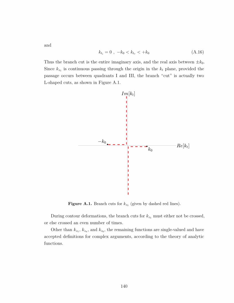
andkti = 0 , −k0 < ktr < +k0 (A.16)

Thus the branch cut is the entire imaginary axis, and the real axis between ±k0.Since kz1 is continuous passing through the origin in the kt plane, provided thepassage occurs between quadrants I and III, the branch “cut” is actually twoL-shaped cuts, as shown in Figure A.1.

Figure A.1. Branch cuts for kz1 (given by dashed red lines).

During contour deformations, the branch cuts for kz1 must either not be crossed,or else crossed an even number of times.

Other than kz1 , kza , and kzb, the remaining functions are single-valued and have

accepted definitions for complex arguments, according to the theory of analyticfunctions.

140

Appendix B|Method of Moments MATLABCode

1 f unc t i on [ Zin , e f f , Gain ] = MoM_Anisotropic (mut ,muz , epst , epsz,W,H, l , check )

2 % This func t i on computes a method o f moments s o l u t i o n o f3 % the mi c r o s t r i p d ipo l e o f l ength L and width W, f o r4 % which L>>W. The d ipo l e l i e s over a magneto−d i e l e c t r i c5 % subs t r a t e o f t h i c kne s s H, d i r e c t i o n a l p e rme ab i l i t i e s6 % mut and muz , d i r e c t i o n a l p e rm i t t i v i t i e s epst and epsz .7 %8 % Inputs :9 % mut ,muz , epst , epsz ( permeab i l i ty , p e rm i t t i v i t y )

10 % vec to r s : W, l ,H (width , length , sub s t r a t e th i ckne s s )11 % boolean : check ( s e t to 1 to d i sp l ay i n t e r n a l checks )12 %13 % Outputs : Zin ( input impedance vs l )14 % e f f ( r ad i a t i on e f f i c i e n c y vs l )15 % Gain ( d i r e c t i v e gain at theta = 0 vs l )16 %17

18 %% Open a prog r e s s bar19

20 wait_bar = waitbar (0 , ’ Progres s ’ ) ;

141

21

22 %% Enter fundamental cons tant s23

24 j = sq r t (−1) ;25 eta0 = 376 .7303113461 ;26 k0 = 2∗ pi ;27

28 %% I n i t i a l i z e v a r i a b l e s29

30 Zin = ze ro s (1 , l ength ( l ) ) ;31 Prad = ze ro s (1 , l ength ( l ) ) ;32 Ptot = ze ro s (1 , l ength ( l ) ) ;33 Prad_check = ze ro s (1 , l ength ( l ) ) ;34 Ptot_check = ze ro s (1 , l ength ( l ) ) ;35 e f f = ze ro s (1 , l ength ( l ) ) ;36 Gain = ze ro s (1 , l ength ( l ) ) ;37

38 f o r b = 1 : l ength ( l )39 %% Grab dimensions o f d i po l e and subs t r a t e from input

ve c t o r s40

41 w = W(b) ;42 h = H(b) ;43 L = l (b) ;44

45 %% Calcu la te number o f ba s i s funct i ons , segment l ength andpo s i t i o n

46

47 N = max(10 , c e i l ( l (b ) / . 02 ) ) ;48 i f mod(N, 2 )==049 N=N+1;50 end51 d = L/(N+1) ;52 x = d ∗ ( 0 : (N−1) )+d ;

142

53

54 %% Precompute i nva r i an t por t i on o f Kernel f o r impedancematrix i n t e g r a l s

55

56 kh = 0.5∗ j ∗k0 ;57 k = 1.1∗max( sq r t (mut∗ epsz ) , s q r t ( epst ∗muz) ) ∗k0 ;58 kx0 = [ l i n s p a c e (0 , kh , 1 0 ) , l i n s p a c e (kh , k+kh , 100 ) , . . .59 l i n s p a c e (k+kh , k , 1 0 ) , l i n s p a c e (k ,3∗ pi /d/2 ,100) ] ;60 ky0 = [ l i n s p a c e (0 , kh , 1 0 ) , l i n s p a c e (kh , k+kh , 100 ) , . . .61 l i n s p a c e (k+kh , k , 1 0 ) , l og space ( log10 (k ) , log10 (3∗ pi /w

/2) ,50) ] ;62 [ kx , ky]=meshgrid ( kx0 , ky0 ) ;63 kx2 = kx .∗ kx ;64 ky2 = ky .∗ ky ;65 kt2 = kx.^2+ky . ^ 2 ;66 k02 = k0 ^2;67 kz1 = sqr t2 ( k02−kt2 ) ;68 kzb = sqr t2 (mut∗ epst ∗k02−mut/muz∗kt2 ) ;69 kza = sqr t2 (mut∗ epst ∗k02−epst / epsz ∗kt2 ) ;70 Gtm = kza .∗ kz1 .∗ kx2 . / ( epst ∗kz1 .∗ cot ( kza∗h)+j ∗kza ) . / kt2 /

k0 ;71 Gte = mut∗k0∗ky2 . / ( j ∗mut∗kz1+kzb .∗ cot ( kzb∗h) ) . / kt2 ;72 A = j ∗ eta0 /4/ p i / p i ;73 fky = s i n c ( ky∗w/2/ pi ) ;74 fkx = d∗ s i n c ( kx∗d/2/ p i ) . ^ 2 ;75 Kmn =A∗(Gtm+Gte ) . ∗ ( fkx .∗ fky ) . ^ 2 ;76 Kmn(1 , 1 ) = A∗d∗d/( j+sq r t ( epst /mut) ∗ cot ( s q r t (mut∗ epst ) ∗

k0∗h) ) ;77

78 %% Precompute i nva r i an t por t i on o f Kernel up to k079

80 kx1 = l i n s p a c e (0 , k0 , 4 0 ) ;81 ky1 = kx1 ;82 [ kx1 , ky1]=meshgrid ( kx1 , ky1 ) ;

143

83 kx2 = kx1 .∗ kx1 ;84 ky2 = ky1 .∗ ky1 ;85 kt2 = kx1.^2+ky1 . ^ 2 ;86 k02 = k0 ^2;87 kz1 = sqr t2 ( k02−kt2 ) ;88 kzb = sqr t2 (mut∗ epst ∗k02−mut/muz∗kt2 ) ;89 kza = sqr t2 (mut∗ epst ∗k02−epst / epsz ∗kt2 ) ;90 Gtm = kza .∗ kz1 .∗ kx2 . / ( epst ∗kz1 .∗ cot ( kza∗h)+j ∗kza ) . / kt2 /

k0 ;91 Gte = mut∗k0∗ky2 . / ( j ∗mut∗kz1+kzb .∗ cot ( kzb∗h) ) . / kt2 ;92 A = j ∗ eta0 /4/ p i / p i ;93 fky = s i n c ( ky1∗w/2/ pi ) ;94 fkx = d∗ s i n c ( kx1∗d/2/ p i ) . ^ 2 ;95 Kmn_rad =A∗(Gtm+Gte ) . ∗ ( fkx .∗ fky ) . ^ 2 ;96 Kmn_rad(1 , 1 ) = A∗d∗d/( j+sq r t ( epst /mut) ∗ cot ( s q r t (mut∗

epst ) ∗k0∗h) ) ;97 kx1 = l i n s p a c e (0 , k0 , 4 0 ) ;98 ky1 = kx1 ;99

100 %% Calcu la te impedance matrix e lements101

102 f i r s t_row = ze ro s (1 ,N) ;103 f i rst_row_rad = ze ro s (1 ,N) ;104

105 f o r n=1:N106 G = 4∗ cos ( kx ∗( x (n)−x (1 ) ) ) .∗Kmn;107 G_rad = 4∗ cos ( kx1 ∗( x (n)−x (1 ) ) ) .∗Kmn_rad ;108 f i r s t_row (n) = trapz ( kx0 , t rapz ( ky0 ,G, 1 ) ) ;109 f i rst_row_rad (n) = trapz ( kx1 , t rapz ( ky1 ,G_rad , 1 ) ) ;110 end111

112 Zpq = t o e p l i t z ( f i r s t_row , f i r s t_row ) ;113 Z_rad = t o e p l i t z ( f irst_row_rad , f i rst_row_rad ) ;114

144

115 %% Create vo l tage column116

117 Vp = ze ro s (N, 1 ) ;118 Vp( (N+1)/2) = 1 ;119

120 %% Solve f o r cur r ent amplitude121

122 Iq = Zpq\Vp;123

124 %% Determine input impedance125

126 Zin (b) = 1/ Iq ( (N+1)/2) ;127

128 %% Determine t o t a l power us ing c i r c u i t theory129

130 Ptot_check (b) = 0.5∗ r e a l ( Iq ( (N+1)/2) ) ;131

132 %% Determine t o t a l power us ing Poynting ’ s theorem133

134 Ptot (b) = 0.5∗ r e a l ( Iq ’∗Zpq∗ Iq ) ;135

136 %% Determine rad ia t ed power us ing Poynting ’ s theorem137

138 Prad (b) = 0.5∗ r e a l ( Iq ’∗Z_rad∗ Iq ) ;139

140 %% Determine e f f i c i e n c y141

142 e f f (b ) = Prad (b) /Ptot (b) ;143

144 %% Compute Poynting vec to r vs ang le145

146 theta = l i n s p a c e (0 , p i /2 ,100) ;147 phi = l i n s p a c e (0 ,2∗ pi , 1 00 ) ;148 [ Theta , Phi ] = meshgrid ( theta , phi ) ;

145

149 s = s i n (Theta ) ;150 c = cos (Theta ) ;151 kza = k0∗ s q r t ( epst ∗mut−epst / epsz ∗ s .^2 ) ;152 kzb = k0∗ s q r t ( epst ∗mut−mut/muz∗ s .^2 ) ;153 kz1 = k0∗c ;154 kx = k0∗ s .∗ cos ( Phi ) ;155 ky = k0∗ s .∗ s i n ( Phi ) ;156 sa = s i n ( kza∗h) ;157 ca = cos ( kza∗h) ;158 sb = s i n ( kzb∗h) ;159 cb = cos ( kzb∗h) ;160 TEs = j ∗mut∗kz1 .∗ sb+kzb .∗ cb ;161 TMs = epst ∗kz1 .∗ ca+j ∗kza .∗ sa ;162 fky = s i n c ( ky∗w/2/ pi ) ;163 fkx = d∗ s i n c ( kx∗d/2/ p i ) . ^ 2 ;164 Js = Theta−Theta ;165 f o r n = 1 : l ength (x )166 Js = Js+Iq (n) ∗exp ( j ∗kx∗x (n) ) ;167 end168 Js = Js .∗ fkx .∗ fky ;169 Etheta = k0∗ eta0 ∗c .∗ cos ( Phi ) .∗ kza .∗ sa .∗ Js . /TMs/2/ p i ;170 Ephi = −k0∗ eta0 ∗mut∗ s i n ( Phi ) .∗ kz1 .∗ sb .∗ Js . /TEs/2/ p i ;171 magE = abs ( Etheta ) .^2+abs ( Ephi ) . ^ 2 ;172 Srad = 0.5/ eta0 ∗magE ;173

174 %% Compute rad ia t ed power by i n t e g r a t i n g Srad175

176 Prad_check (b) = trapz ( theta , t rapz ( phi , s .∗ Srad , 1 ) ) ;177

178 %% Calcu la te D i r e c t i v e Gain in Forward d i r e c t i o n179

180 Gain (b) = 10∗ l og10 (4∗ pi ∗Srad (1 , 1 ) /Ptot (b) ) ;181

182 %% Update p rog r e s s bar

146

183

184 waitbar (b/ l ength ( l ) )185

186 end187

188 %% Close p rog r e s s bar189

190 c l o s e ( wait_bar ) ;191

192 i f check == 1193

194 %% Compare Ptot computed two ways195

196 f i g u r e ( ) ;197 p lo t ( l , Ptot , ’b ’ , ’ l i n ew id th ’ , 1 . 5 )198 hold on199 p lo t ( l , Ptot_check , ’−−r ’ , ’ l i n ew id th ’ , 1 . 5 )200 t i t l e ( ’Compare t o t a l power c a l c u l a t ed 2 d i f f e r e n t ways ’

)201 l egend ( ’ Equation ( 5 . 4 4 ) ’ , ’ Equation ( 5 . 3 9 ) ’ )202

203 %% Compare Prad computed two ways204

205 f i g u r e ( ) ;206 p lo t ( l , Prad , ’b ’ , ’ l i n ew id th ’ , 1 . 5 )207 hold on208 p lo t ( l , Prad_check , ’−−r ’ , ’ l i n ew id th ’ , 1 . 5 )209 t i t l e ( ’Compare rad ia t ed power c a l c u l a t ed 2 d i f f e r e n t

ways ’ )210 l egend ( ’ Equation ( 5 . 4 6 ) ’ , ’ I n t e g r a t i n g Poynting Vector

in Far F i e ld ’ )211

212 end213

147

214 end

1 f unc t i on w = sqr t2 ( z )2

3 j = sq r t (−1) ;4 r = abs ( z ) ;5 theta = angle ( z ) ;6 theta ( theta <=0) = theta ( theta <=0)+2∗pi ;7 w = −s q r t ( r ) .∗ exp ( j ∗ theta /2) ;8

9 end

148

Appendix C|Comparisons to FEKO for anIsotropic Substrate

Commercially available solvers, for example FEKO [66], can handle isotropicmagneto-dielectric substrates. The models developed in this dissertation incorporateanisotropy in both the permeability and permittivity of the magneto-dielectricsubstrate, which is a capability that is not available in FEKO. Assuming FEKO iscorrectly implemented, we expect our model’s results to agree with FEKO in thespecial case that the substrate is made isotropic. In this appendix, we perform thisverification.

In Chapter 5, we considered the example of an isotropic substrate of µr = 50,εr = 3, and W = h = L/12.5, and calculated the input impedance versus L. InFigure C.1 and Figure C.2, the input impedance and directive gain calculated bythe algorithm described in Chapter 5 is compared to results exported from FEKO.The agreement in Figure C.2 for the directive gain is excellent. The agreementin input impedance is also very good, but not perfect. This is not surprising, asthe input impedance is more sensitive to the discretization near the source regionthan the gain. In FEKO, surface mesh elements defined over triangular domainsare utilized. For simplicity, our model utilizes surface mesh elements defined overrectangular domains. The discretization in FEKO is obtained by setting the edgelength of the triangular domains to be L/20, as pictured in Figure C.3. An edgeport is used for the excitation, as pictured (in blue and red colors) straddling thebisector of the dipole in Figure C.3.

149

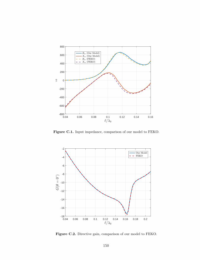
0.04 0.06 0.08 0.1 0.12 0.14 0.16-800

-600

-400

-200

0

200

400

600

800

Figure C.1. Input impedance, comparison of our model to FEKO.

0.04 0.06 0.08 0.1 0.12 0.14 0.16 0.18 0.2-18

-16

-14

-12

-10

-8

-6

-4

-2

Figure C.2. Directive gain, comparison of our model to FEKO.

150

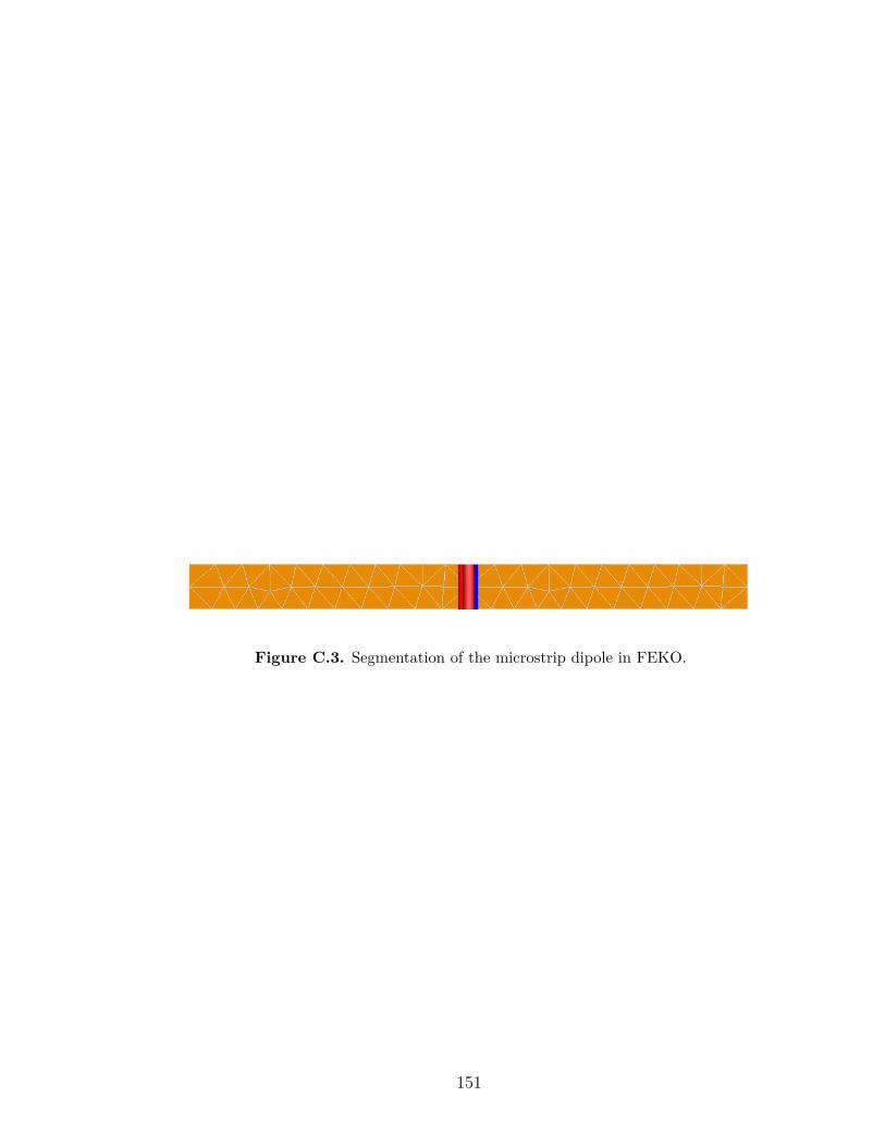
Figure C.3. Segmentation of the microstrip dipole in FEKO.

151

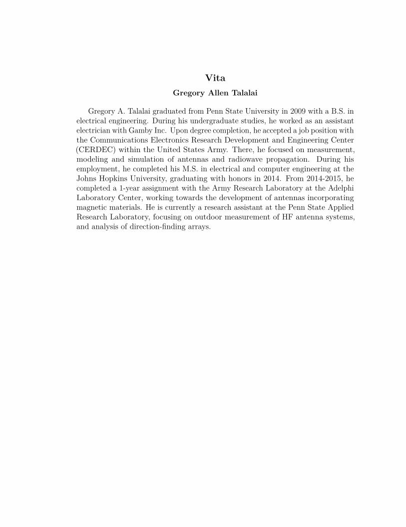
VitaGregory Allen Talalai

Gregory A. Talalai graduated from Penn State University in 2009 with a B.S. inelectrical engineering. During his undergraduate studies, he worked as an assistantelectrician with Gamby Inc. Upon degree completion, he accepted a job position withthe Communications Electronics Research Development and Engineering Center(CERDEC) within the United States Army. There, he focused on measurement,modeling and simulation of antennas and radiowave propagation. During hisemployment, he completed his M.S. in electrical and computer engineering at theJohns Hopkins University, graduating with honors in 2014. From 2014-2015, hecompleted a 1-year assignment with the Army Research Laboratory at the AdelphiLaboratory Center, working towards the development of antennas incorporatingmagnetic materials. He is currently a research assistant at the Penn State AppliedResearch Laboratory, focusing on outdoor measurement of HF antenna systems,and analysis of direction-finding arrays.