Embed Size (px)
Citation preview
Theory and Problems of Fundamentals of Computing with C++
John R. Hubbard, Ph.D.
Professor of Mathematics and Computer Science University of Richmond
SCHAUM'S OUTLINE SERIES McGraw HillNew York San Francisco Washington, DC
Auckland Bogata Caracas Lisbon London Madrid Mexico City Milan Montreal New Delhi San Juan Singapore, Sydney Tokyo Toronto
JOHN R. HUBBARD is Professor of Mathematics and Computer Science at the University of Richmond. He received his Ph.D. from The University of Michigan (1973) and has been a member of the Richmond faculty since 1983. His primary interests are in numerical algorithms and database systems. Dr. Hubbard is the author of several other books, including Schaum's Outline of Programming with C++.
Schaum's Outline of Theory and Problems of PROGRAMMING
WITH C++
Copyright © 1998 by The McGraw-Hill Companies, Inc. All rights reserved. Printed in the United States of America. Except as permitted under the Copyright Act of 1976, no part of this publication may be reproduced or distributed in any form or by any means, or stored in a data base or retrieval system, without the prior written permission of the publisher.
2 3 4 5 6 7 8 9 10 11 12 13 14 15 16 17 18 19 20PRSPRS 9 0 1 0 9 8
ISBN 0-07-030868-3
Sponsoring Editor: Barbara Gilson Production Supervisor: Sherri Souffrance Editing Supervisor: Maureen Walker
Library of Congress Cataloging-in-Publication Data
Hubbard, J. R. (John R.), date Schaum's outline of theory and problems of fundamentals of computing with C++ / John R. Hubbard. p. cm. — (Schaum's outline series) Includes bibliographical references and index. ISBN 0-07-030868-3 (pbk.) 1. C++ (Computer program language) 2. Computer science. 1. Title II. Series QA76.73.C153H82 1998
Preface□Like all Schaum's Outline Series books, this is intended to be used primarily for self study, preferably in conjunction with a regular course in the fundamentals of computer science using the new ANSI/ISO Standard C++. The book covers topics from the following fundamental units of the 1991 A.C.M. Computing Curricula:
AL1: Basic Data Structures AL2: Abstract Data Types AL3: Recursive Algorithms AL4: Complexity Analysis AL5: Complexity Classes AL6: Searching and Sorting
The book includes over 500 examples and solved problems. The author firmly believes that computing is learned best by practice, following a well-constructed collection of examples with complete explanations. This book is designed to provide that support.
Source code for the examples and solved problems in this book may be downloaded from the author's World Wide Web home page: http://www.richmond.edu/~hubbard/
This site will also contain any corrections and addenda for the book.
I wish to thank all my friends, colleagues, students, and the McGraw-Hill staff who have helped me with the critical review of this manuscript. Special thanks to Anita Hubbard, Jim Simons, and Maureen Walker. Their debugging skills are gratefully appreciated.
JOHN R. HUBBARD RICHMOND, VIRGINIA
Dedicated to my 1997 computer science students:
Miriam Albin, Allison Bannon, Carolyn Bennett, Ben Brown, Jon-Eric Burgess, Andre Chambers, Kenric Chu, Danielle Clement, Jim Copenhafer, Mark DeSantis, JohnM. Ewing, John R. Ewing, Jeff Frick, Shannon Greening, Russ Haskin, Kevin Hawkins, Hunt Hejfner, John Hettler, William Hooker, Sara Hoopengardner, Tim Hospodar, Michelle Hucher, Rob Hunt, Rob James, Tony Kirilusha, Brian Magliaro, Joel Mascardo, Marc Meulener, Cavan Miller, Nick Gardiakos, Brock Parker, Jeremy Perella, Betsy Plunket, Kathleen Ribeiro, Christian Schwarzkopf, Chris Severino, Randy Shehady, Jim Simons, Mike Smith, Heather Smucker, Ted Solley, Sarah Spence, Seef Syed, David Vermette, John Vitale, John Wells, Brian Williams, and Josh Youn

Contents □ Chapter 1 1 Introduction to Computing
1.1 A Brief History of Computing 1
1.2 Computer Hardware 3
1.3 Binary Numerals 4
1.4 Computer Storage 6
1.5 Operating Systems 8
1.6 File Systems 9
1.7 Software Development 10
Chapter 2 24 C++ Fundamentals
2.1 The "Hello World" Program 24
2.2 Variables and Declarations 25
2.3 Keywords and Identifiers 26
2.4 Input and Output 27
2.5 Expressions and Operators 27
2.6 Initializations and Constants 29
2.7 Standard C++ Data Types 29
2.8 Enumeration Types 31
2.9 The Standard Library 32
2.10 Errors 33
Chapter 3 43
Control Structures
3.1 Blocks and Scope 43
3.2 Namespaces 44
3.3 The if and if...else Statements 45
3.4 The Conditional Expression Operator 47
3.5 Operators 47
3.6 The while Statement 49
3.7 The do. . . While Statement 50
3.8 The for Statement 51
3.9 The break and cont inue Statements 52
3.10 Loop Invariants 53
3.11 Nested Loops 54
Chapter 4 67 Functions
4.1 Function Declarations and Definitions 67
4.2 void Functions 69
4.3 Tracing a Function 70
4.4 Test Drivers 70
4.5 Using The assert() Function to Check Preconditions 71
4.6 Predicates 72
4.7 Default Arguments 73
4.8 Pass by Const Value, by Reference, and Const Reference 74
4.9 Returning by Reference 76
4.10 Overloading a Function Name 77
Chapter 5 88 Arrays
5.1 Defining and Traversing Arrays 88
5.2 Initializing an Array 89
5.3 Duplicating an Array 89
5.4 Constant Arrays 90
5.5 Array Index Out of Range 90
5.6 The sizeof Operator 91
6.7 Passing an Array to a Function 92
6.8 Applications of Arrays 93
6.9 Two-Dimensional Arrays 96
6.10 Machine Storage of Arrays 98
Chapter 6 109 Strings and Files
6.1 C-Strings 109
6.2 The <cstring> Library 110
6.3 Formatted Input 112
6.4 Unformatted Input 113
6.5 The s tr ing Type 114
6.6 Files 116 6.7 String Streams 114
6.8 Random Access Files 119
Chapter 7 137
Abstract Data Types
7.1 Procedural Abstraction 137
7.2 Function Templates 140
7.3 Data Abstraction 141
7.4 C ++ Friend Functions 143
7.5 Overloading Operators 145
7.6 Class in Variants 147
7.7 Constructors and Destructors 149
7.8 The Four Automatic Member Functions 151
7.9 Abstract Data Types 153
Chapter 8 178
Pointers
8.1 Pointers 178
8.2 The Dereference Operator 178
8.3 Pointer Operations 179
8.4 The Reference Operator 182
8.5 Null Pointers 184
8.6 Dynamic Arrays 185
8.7 The th is Pointer 188
Chapter 9 195 Lists
9.1 Linked Structures 195
9.2 C++ StructsD 196
9.3 Linked Inplementation of the Stack ADT 198
9.4 Iterators 200
9.5 A List ADT 202
9.6 A List Class 204
Chapter 10 226 Standard Container Classes
10.1 Containers 226
10.2 Templates 226
10.3 Standard C++ Container Classes and Their Operations 228
10.4 The C++ Standard Stack Class Template 231
10.5 The C++ Standard Queue Class Template 232
10.6 The C++ Standard Vector Class Template 234
10.7 The C++ Standard Lis t Class Template 236
10.8 Generic Algorithms 239
Chapter 11 254 Recursion
11.1 Introduction 254
11.2 The Basis for a Recursive Definition 254
11.3 Implementations of the factor ia l () Function 255
11.4 Activation Frames 256
11.5 The Fibonacci Sequence 257
11.6 The Euclidean Algorithm 258
11.7 The Recursive Binary Search 259
11.8 The Towers of Hanoi 261
11.9 Mutual Recursion 262
11.10 Backus-Naur Form 264
Chapter 12 276
Trees
12.1 General Trees 276
12.2 Binary Trees 277
12.3 Tree Traversals 279
12.4 Expression Trees 281
12.5 ADTs for Binary Trees and Their Iterators 283
12.6 Contiguous Implementation 285
12.7 Linked Implementation 290
12.8 Forests 292
Chapter 13 303
Sorting
13.1 Preliminaries 303
13.2 The Bubble Sort 303
13.3 The Selection Sort 306
13.4 The Insertion Sort 307
13.5 The Merge Sort 308
13.6 The Quick Sort 310
13.7 Heaps 311
13.8 The Heap Sort 312
Chapter 14 319 Searching
14.1 The Sequential Search Algorithm 319
14.2 The Standard C++ f ind () Function Templates 320
14.3 The Binary Search Algorithm 320
14.4 Binary Search Trees 322
14.5 AVL Trees 323
14.6 Hash Tables 324
14.7 Searching A Hash Table 329
14.8 Collision-Resolution Algorithms 332
Appendix A 340
Algorithms
Appendix B 341
References Index 350
Chapter 1
Introduction to Computing
1.1 A BRIEF HISTORY OF COMPUTING
Computing is a human process. It involves recognizing and clarifying a problem, devising a method for solving the problem, executing the solution, and then correcting and revising the solution. A computer is a mechanical device that facilitates the last two stages of this process. These days computers are electronic devices that can perform tasks millions to billions times faster than humans. But they are still just mechanical devices designed and built by humans.
Usually the most difficult part of computing is the second stage of the process: devising a method for solving the problem. The resulting method is called an algorithm, which is a step-by-step procedure that can be carried out automatically by a computer. Here is a simple example of an algorithm, discovered by the ancient Babylonians over 4000 years ago:
Algorithm 1.1 The Babylonian Algorithm for Computing the Square Root of 2
This is the algorithm that the ancient Babylonians used to compute the square root of two (V2):
1. Set y = 1.0.
2. Replace y with the average of y and 2/y.
3. Repeat Step 2 until its effect upon y is insignificant.
4. Return y.
EXAMPLE 1.1 The Babylonian Algorithm The Babylonians and the Egyptians apparently used this algorithm to lay square foundations for their
buildings. It remains to this day the best way to compute the square root of 2. Here are the resulting calculations using a 12-digit calculator:
Square the answer to see that it is correct: (1.41421356237)2 = 1.99999999999 = 2.0000000000.
The history of computing is even older than the Babylonian Algorithm. Indeed it is fair to say that computing began with simple counting. The first computing devices were the fingers on a hand. We still use the word "digit" (meaning "finger") to describe the symbols "4", "9", etc. that we use for numbers. The simple task of counting is a common task modern computers perform.
y 2/y (y + 2/y)/2
1.0 1.5 1.4166666667 1.41421568628 1.41421356238 1.41421356237
2.0 1.33333333333 1.41176470588 1.41421143847 1.41421356237 1.41421356237
1.5 1.41666666667 1.41421568628 1.41421356238 1.41421356237 1.41421356237

Another prehistoric computing device that is still in use today is the abacus. This Oriental device allows rapid addition and subtraction by sliding beads along parallel wires held in a frame. Experienced users of the abacus can often outperform western shoppers using a modern calculator.
The first mechanical calculator was designed and built by the German mathematician Wilhelm Schickard (1592-1635) in 1623. It was capable of addition, subtraction, multiplication, and division. But in 1624 his only working copy was destroyed in a fire. Schickard and his entire family perished in the plagues brought on by the Thirty Years War. His design was not discovered until 1957 when his complete description with sketches were found in a letter to Kepler.
Because Schickard's achievement went unnoticed by historians, the French mathematician Blaise Pascal (1623-1662) is usually credited with inventing the first calculator. Capable of only addition and subtraction, this device was inferior to Schickard's calculator. But Pascal was actually successful in marketing his device, and several of them exist to this day.
The great German mathematician Gottfried Wilhelm Leibniz (1646-1716) expanded upon Pascal's idea, building a calculator in 1673 known as the Leibniz wheel. It completely automated all the four basic arithmetic operations: addition, subtraction, multiplication, and division. Leibniz had one copy of his machine built for Peter the Great to send to the Emperor of China.
The first modern computer was designed by the English mathematician Charles Babbage (1791- 1871). He actually designed two computing devices: his Difference Engine in 1823 and his Analytical Engine in 1833. The Difference Engine was designed to tabulate tables of functions using the method of finite differences. There was a genuine need in England for such a machine: British navigational tables of the time, upon which British shipping depended, were rife with human errors. Babbage recognized that completely accurate tables could be constructed automatically "by steam." But before the construction of his Difference Engine could be completed, Babbage abandoned it in favor of a much better machine: his Analytical Engine. This would be the first truly general purpose programmable computer with its own processor, memory, secondary storage, input device, and output device. The programs would be stored on a belt of punched paste cards, the same way that Joseph Marie Jacquard's loom stored programs for patterns to be weaved into fabrics.
The idea of using punched cards was taken up by the American engineer Herman Hollerith (1860-1929). In 1889 he contracted with the U.S. Census Bureau to process the 1890 census data automatically. He invented an electronic tabulating machine which was a great success. In 1896 Hollerith established the Tabulating Machine Company, which later evolved into the International Business Machine company (IBM).
The next major achievement in the history of computing occurred in 1939 at Harvard University when Howard H. Aiken persuaded IBM to support a project to build a modernized version of Babbage's Analytical Engine. Building upon the already-successful punch-card business machines marketed by IBM, Aiken wanted to build a computer that would do for science what IBM's machines were doing for business. When completed in 1944, the Mark I electromechanical computer was able to perform automatically scientific computations with far greater speed and accuracy than had been possible previously. It stored its programs on punched tape, similar to Jacquard's belts of punched paste cards.
Near end of the Second World War, John W. Mauchly and J. Presper Eckert, Jr. designed and built the Electronic Numerical Integrator and Computer (ENIAC). This huge machine was the first electronic digital computer. It was built to tabulate firing tables for the U.S. Army. After the war, Mauchly and Eckert formed a private company which built and marketed the Universal Automatic Computer (UNIVAC), the first commercial computer designed for both business and scientific applications. The first one was bought by the U.S. Census Bureau in 1951.
Charles Babbage had borrowed Jacquard's idea of storing programs on external punch cards. But it was the great Hungarian-American mathematician John von Neumann who thought of storing programs in the computer's memory itself, the same way that data is stored. He suggested this idea in 1945 and incorporated it into the design of the IAS (Institute for Advanced Study) computer which became the basis for the design of all modern computers.
Computers in the 1940s used vacuum tubes to store data. These were unreliable, took up a lot of space, and consumed a lot of electricity. In the 1950s, vacuum tubes were replaced by magnetic core memory. This consisted of tiny magnetic rings threaded on wire mesh racks. The transition made computer memory faster, cheaper, and more compact.
In 1948 at Bell Labs, William Shockley and associates invented the transistor, a tiny electrical device that transfers electrical signals across a resistor. These were found to be effective devices for storing and processing data electronically, and by 1959 were replacing magnetic core memory.
Around 1965, fabrication plants in Santa Clara, California were successful in replacing individual transistors with integrated circuits impressed on a silicon chip. This region, now called Silicon Valley, has become a world center of microcomputer technology. Progress in the VLSI (very large scale integration) of integrated circuits on silicon microchips has been continuous and dramatic.
In 1974, the Intel Corporation released its 8080 microprocessor. This inexpensive CPU (central processing unit) made the microcomputer possible. Progress in microcomputer technology can be measured by the successors to the i8080: the i8086 in 1977, the i80286 in 1984, the i80386 in 1986, the i80486 in 1989, the Pentium (also called the i80586) in 1993, and the Pentium II in 1996.
In the 1960s the U.S. Defense Department developed a nationwide computer network called ARPANet (Advanced Research Projects Agency Network) to facilitate communication among its researchers. This network later expanded and combined with other networks, and evolved into today's Internet. In 1990 Tim Berners-Lee, working at the CERN laboratory in Switzerland developed software that made it easy to link to distant computers on the Internet and to send email (electronic mail). His work marks the beginning of the World Wide Web.
The unprecedented growth in the computer industry in the past 50 years is difficult to overstate. A new generation of technology appears about every three years which makes computing much faster, easier, and cheaper. In less than 50 years, the computer industry has become the third largest sector of the world economy (after energy and illegal drugs). It has been observed that if the automobile industry had developed as fast, we would now be able to purchase a car for under a dollar that could take us to the moon and back in a few minutes.
1.2 COMPUTER HARDWARE
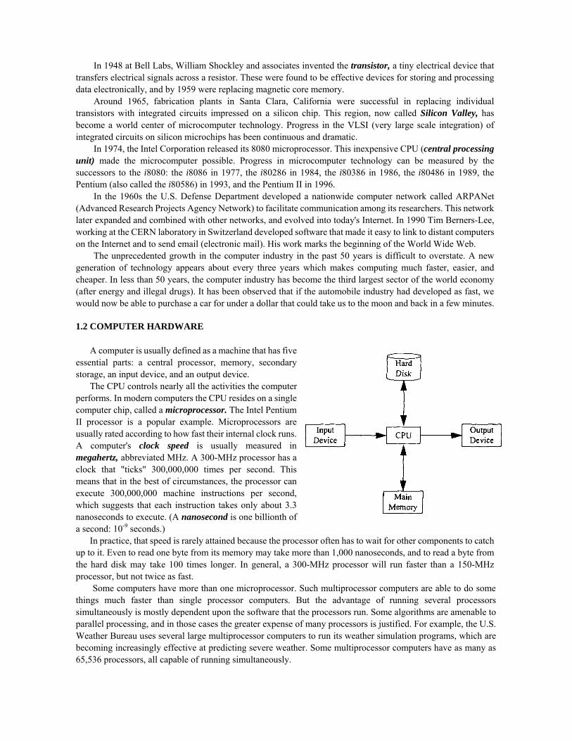
A computer is usually defined as a machine that has five essential parts: a central processor, memory, secondary storage, an input device, and an output device.
The CPU controls nearly all the activities the computer performs. In modern computers the CPU resides on a single computer chip, called a microprocessor. The Intel Pentium II processor is a popular example. Microprocessors are usually rated according to how fast their internal clock runs. A computer's clock speed is usually measured in megahertz, abbreviated MHz. A 300-MHz processor has a clock that "ticks" 300,000,000 times per second. This means that in the best of circumstances, the processor can execute 300,000,000 machine instructions per second, which suggests that each instruction takes only about 3.3 nanoseconds to execute. (A nanosecond is one billionth of a second: 10-9 seconds.)
In practice, that speed is rarely attained because the processor often has to wait for other components to catch up to it. Even to read one byte from its memory may take more than 1,000 nanoseconds, and to read a byte from the hard disk may take 100 times longer. In general, a 300-MHz processor will run faster than a 150-MHz processor, but not twice as fast.
Some computers have more than one microprocessor. Such multiprocessor computers are able to do some things much faster than single processor computers. But the advantage of running several processors simultaneously is mostly dependent upon the software that the processors run. Some algorithms are amenable to parallel processing, and in those cases the greater expense of many processors is justified. For example, the U.S. Weather Bureau uses several large multiprocessor computers to run its weather simulation programs, which are becoming increasingly effective at predicting severe weather. Some multiprocessor computers have as many as 65,536 processors, all capable of running simultaneously.
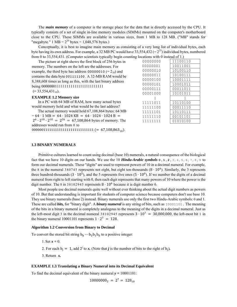
The main memory of a computer is the storage place for the data that is directly accessed by the CPU. It typically consists of a set of single in-line memory modules (SIMMs) mounted on the computer's motherboard close to the CPU. These SIMMs are available in various sizes, from 1 MB to 128 MB. ("MB" stands for "megabyte." 1 MB = 220 bytes = 1,048,576 bytes.)
Conceptually, it is best to imagine main memory as consisting of a very long list of individual bytes, each byte having its own address. For example, a 32 MB PC would have 33,554,432 (= 225) individual bytes, numbered from 0 to 33,554,431. (Computer scientists typically begin counting locations with 0 instead of 1.)
The picture at right shows the first block of 256 bytes in memory. The numbers on the left are the addresses. For example, the third byte has address 00000010 (= 210) and contains the data byte 001111100. A 32-MB RAM would be 8,388,608 times as long as this, with the last binary address being 00000001111111111111111111111111 (= 33,554,43110).
EXAMPLE 1.2 Memory size In a PC with 64 MB of RAM, how many actual bytes
would memory hold and what would be the last address? The actual memory would hold 67,108,864 bytes: 64 MB
= 64 ⋅ 1 MB 64 ⋅ 1024KB 64 ⋅ 1024 ⋅ 1024B2 ⋅ 2 ⋅ 2 2 67,108,864 bytes of memory. The addresses would run from 0 to 00000011111111111111111111111111 67,108,86310 .
00000000 11100110 00000001 10011001 00000010 10100110 00000011 10100111 00000100 10001111 00000101 10001011 00000111 00011011 00001000 10101011
⋮ ⋮ 11111011 10110100 11111100 00011110 11111101 10110111 11111110 00101101 11111111 01010100
1.3 BINARY NUMERALS
Primitive cultures learned to count using decimal (base 10) numerals, a natural consequence of the biological fact that we have 10 digits on our hands. We use the 10 Hindu-Arabic symbols 0,1,2,3,4,5,6,7,8,9 to form our decimal numerals. These "digits" are used to represent powers of 10 in a decimal numeral. For example, the 8 in the numeral 380745 represents not eight, but eight ten-thousands (8 ⋅ 10 ). Similarly, the 3 represents three hundred-thousands (3 ⋅ 10 ), and the 5 represents five ones (5 ⋅ 10 ). If we number the digits of a decimal numeral from right to left starting with 0, then each digit represents that many powers of 10 where the power is the digit number. The 8 in 38102945 represents 8 ⋅ 10 because it is digit number 6.
Most people use decimal numerals quite well without ever thinking about the actual digit numbers as powers of 10. But that understanding is important for students of computer science because computers don't use base 10. They use binary numerals (base 2) instead. Binary numerals use only the first two Hindu-Arabic symbols: 0 and 1. These are called bits, for "binary digit". A binary numeral is any string of bits, such as 10001101. The meaning of the bits in a binary numeral is completely analogous to the meaning of the digits in a decimal numeral. Just as the left-most digit 3 in the decimal numeral 38102945 represents 3 ⋅ 10 30,000,000, the left-most bit 1 in the binary numeral 10001101 represents 1 ⋅ 2 128.
Algorithm 1.2 Conversion from Binary to Decimal
To convert the stored bit string b ⋯b b b to a positive integer:
1. Set x = 0.
2. For each b 1, add 2j to x. (Note that j is the number of bits to the right of b ).
3. Return x.
EXAMPLE 1.3 Translating a Binary Numeral into its Decimal Equivalent
To find the decimal equivalent of the binary numeral y = 10001101:
10000000 2 128
1000 2 8
100 2 4
1 2° 1 The answer is 128 + 8 + 4 + 1 = 141. The subscripts 2 and 10 are used to designate "binary" and "decimal". So this correspondence can be written 100011012 = 14110.
Translating decimal numerals into binary is not as straightforward as the reverse process. One way to do it is to reverse the algorithm described in Example 1.3: instead of adding powers of 2 to get the decimal numeral, subtract powers of 2 from the given decimal numeral.
The next algorithm has the same effect as Algorithm 1.2, but it uses Horner's Method for greater efficiency. This method factors the sum to replace exponentiation with multiplication. For example, it would perform the operation 128 + 8 + 4 + 1 = 141 as
0 1 ⋅ 2 0 ⋅ 2 0 ⋅ 2 0 ⋅ 2 1 ⋅ 2 1 ⋅ 2 0 ⋅ 2 1 141
Note that the (underlined) bits from original bit string 10001101 appear in order in this expression. Although it looks more complicated, this algorithm is easier to implement and is more efficient.
Algorithm 1.3 Conversion from Binary to Decimal by Horner's Method
This uses Horner's Method to convert the stored bit string bk—b2b\b0 to a positive integer:
1. Set x = 0.
2. Set j = k + 1 (the actual number of bits in the string b ⋯b b b ).
3. Subtract 1 from j.
4. Multiply x by 2.
5. Add bj to x.
6. If j > 0, repeat steps 3-6. 7. Return x.
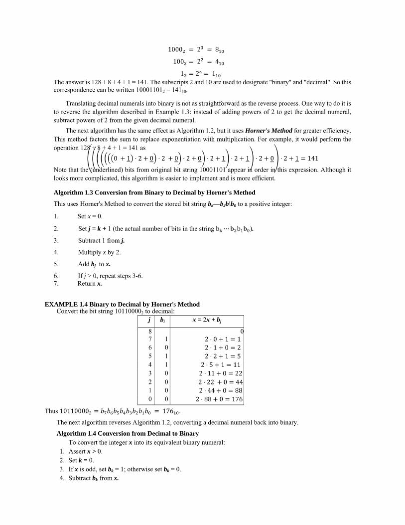
EXAMPLE 1.4 Binary to Decimal by Horner's Method
Convert the bit string 101100002 to decimal:
Thus 10110000 176 .
The next algorithm reverses Algorithm 1.2, converting a decimal numeral back into binary.
Algorithm 1.4 Conversion from Decimal to Binary To convert the integer x into its equivalent binary numeral:
1. Assert x > 0. 2. Set k = 0. 3. If x is odd, set bk = 1; otherwise set bk = 0. 4. Subtract bk from x.
j bi x = 2x + bj
8 07 1 2 ⋅ 0 1 16 0 2 ⋅ 1 0 25 1 2 ⋅ 2 1 54 1 2 ⋅ 5 1 113 0 2 ⋅ 11 0 222 0 2 ⋅ 22 0 441 0 2 ⋅ 44 0 880 0 2 ⋅ 88 0 176
5. Divide x by 2. 6. Add 1 to k. 7. If x > 0, repeat steps 3-6. 8. Return ⋯ .
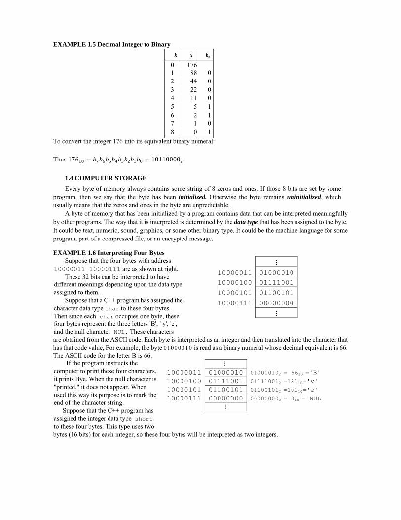
EXAMPLE 1.5 Decimal Integer to Binary
To convert the integer 176 into its equivalent binary numeral:
Thus 176 10110000 .
1.4 COMPUTER STORAGE
Every byte of memory always contains some string of 8 zeros and ones. If those 8 bits are set by some program, then we say that the byte has been initialized. Otherwise the byte remains uninitialized, which usually means that the zeros and ones in the byte are unpredictable.
A byte of memory that has been initialized by a program contains data that can be interpreted meaningfully by other programs. The way that it is interpreted is determined by the data type that has been assigned to the byte. It could be text, numeric, sound, graphics, or some other binary type. It could be the machine language for some program, part of a compressed file, or an encrypted message.
EXAMPLE 1.6 Interpreting Four Bytes Suppose that the four bytes with address
10000011-10000111 are as shown at right. These 32 bits can be interpreted to have
different meanings depending upon the data type assigned to them.
Suppose that a C++ program has assigned the character data type char to these four bytes. Then since each char occupies one byte, these four bytes represent the three letters 'B', ' y', 'e', and the null character NUL. These characters
⋮10000011 01000010
10000100 01111001 10000101 01100101 10000111 00000000
⋮
are obtained from the ASCII code. Each byte is interpreted as an integer and then translated into the character that has that code value, For example, the byte 01000010 is read as a binary numeral whose decimal equivalent is 66. The ASCII code for the letter B is 66.
If the program instructs the computer to print these four characters, it prints Bye. When the null character is "printed," it does not appear. When used this way its purpose is to mark the end of the character string.
Suppose that the C++ program has assigned the integer data type short to these four bytes. This type uses two
⋮ 10000011 01000010 010000102 = 6610 ='B' 10000100 01111001 011110012 =12110='y' 10000101 01100101 011001012 =10110='e' 10000111 00000000 000000002 = 010 = NUL
⋮
bytes (16 bits) for each integer, so these four bytes will be interpreted as two integers.
k x bk
0 176
1 88 02 44 03 22 04 11 05 5 16 2 17 1 08 0 1

As decimal numerals, these two integers are 17,017 and 25,856. Note that 16-bit (signed) integers will be in the range -32,768 to 32,767.
Now suppose that these same four bytes are interpreted with the Standard C++ data type wchar_t. This type uses two bytes (16 bits) for each character, so
⋮
10000011 01000010
10000100 01111001 01000010011110012 = 1701710
10000101 01100101
10000111 00000000 01100101000000002 = 2585610
⋮
these four bytes will be interpreted as two Unicode characters. The first of these two 16-bit characters (Unicode 17,017) is a Chinese glyph.
Another possible interpretation of the same four bytes is as a single 32-bit integer of type int. These four bytes represent the single (decimal) integer 1,115,251,968. Note that, in general, 32-bit (signed) integers range from 2,147,483,648 to 2,147,483,647.
⋮
10000011 01000010
10000100 01111001
10000101 01100101
10000111 00000000 010000100111100101100101000000002 = 1,115,251,96810
⋮ If these four bytes are assigned the C++ floating-point type float, they evaluate to the decimal number
62.34863. The algorithm used for this conversion is complicated. It divides the 32 bits into three parts: the left-most bit is called the sign bit, the next 8 bits form the exponent, and the right-most 23 bits form the fraction. For the 32-bit string 01000010011110010110010100000000, the sign bit is 0 , the exponent is 10000100 , and the fraction is 11110010110010100000000 . These three components determine that the number is positive, it has an exponent value of 10000100 127 132 127 5 , and a fraction value of 1.1111001011001012. That forms the number +1.1111001011001012 x 25 = 111110.01011001012 = 25 + 24 + 23
+ 22 + 21 + 2-2 + 2-4 + 2-5 + 2-8 + 2-10 = 62.34863. Note that 127 is subtracted from the stored 8-bit exponent and 1 is added to the 23-bit fraction. This algorithm is known as the excess-127 floating-point representation.
This example shows that the same four bytes can represent the text "Bye", the four integers {66, 121, 101, 0}, the two integers 17,017 and 25,856, two Unicode characters, the single integer 1,115,251,968, or the single real number 62.34863, depending upon whether the data type is char, unsigned char, short, wchar_t, int, or float. There are several other data types available in C++ that would yield other different values for these same 32 bits.
The correspondences between memory bits and the characters that they represent are called character codes. Standard C++ uses the 8-bit ASCII code and the 16-bit Unicode. ASCII (pronounced "as-key") is an acronym for the American Standard Code for Information Interchange. Unicode is a newer international code that includes all the standard European and Asian characters and many special symbols, such as mathematics and music symbols.
1.5 OPERATING SYSTEMS
There is a special program that is always running when the computer is turned on; it is called its operating system, because it "operates" the computer, controlling all its hardware and software functions. When you turn on your computer, as soon as it finishes running its diagnostic tests, it copies its operating system from its hard disk into its memory and starts it running. This is called booting the system because the computer is getting itself running, like pulling itself up by its bootstraps.
Different computers use different operating systems. The most popular are Windows 95, MacOS, MS-DOS, Windows NT, OS/2, and various dialects of UNIX such as LINUX, Solaris, FreeBSD, AIX, XENIX, HP-UX, IRIX, and NEXTSTEP. Most PCs use Windows 95, most Macintoshes use MacOS, and most workstations use some dialect of UNIX. Since all programs that run on your computer must be controlled by its operating system,

any new software that you install has to be compatible with that system. So most popular software like the Firefox web browser have different versions for the most popular operating systems.
The computer's OS (operating system) controls all the computer's hardware. This is done through the CPU. When you run a program like Firefox, the OS starts the program and remains ready to respond to every request that the program and its client programs make. For example, if you want to read your email you click on a button that requests access to your new mail. That request goes to the OS which looks up where your mail is stored and then returns information (e.g., how many messages there are) to your mail program which then displays it for you.
The most common activity performed by the CPU is simple arithmetic. This is handled by the arithmetic and logic unit (the ALU) which is an internal part of the most modern CPUs. To illustrate how this is done, consider the problem of adding the integers 37 (= 001001012) and 84 (= 010101002). First the CPU fetches these two numbers from memory and loads them into registers which are storage places within the CPU. Then it carries out the addition, placing the sum into another register. Then it stores that answer back into memory. These operations themselves are translated into binary numerals, called opcodes, and stored with the data in memory. The opcodes are appended to the memory addresses of the data, called operands, upon which they operate. For example, if the opcode for the LOAD operation is 16 (= 000100002) and its operand (i.e., the memory address of the number to be loaded) is 97 (= 011000012), then the first machine language instruction would be 0001000000000100, which means "load the number stored at byte number 4 into the accumulator (the register in the CPU where arithmetic is performed). Suppose that the machine language uses the following opcodes:
LOAD 00010000 STORE 00010001 ADD 00100011 MULTIPLY 00100100
Then our complete machine language program would be 0001000001100001 LOAD the number stored at byte #97 0010001101100010 ADD to it the number stored at byte #98 0001000101100011 STORE the result at byte #99 When executed, this program would have the effect shown here:
Of course the 48- bit program will be stored somewhere else in memory. The OS reads each 16-bit instruction one-at-a- time. Each time, the OS "fetches" (i.e.,copies) the instruction into one of its registers, and then executes it. That two-step process is called the fetch-execute cycle. A 120-MHz CPU can do that 120,000,000 times per second.So it would take that CPU about 25 nanoseconds (3x1/120,000,000 seconds) to perform the addition 37 + 84 = 121.
The 3-line machine language program above would be written in assembly language as LOAD A ADD B STORE C
where A and B are symbolic names for the addresses where 37 and 84 are stored, and C is a symbolic name for the address where the sum is to be stored.
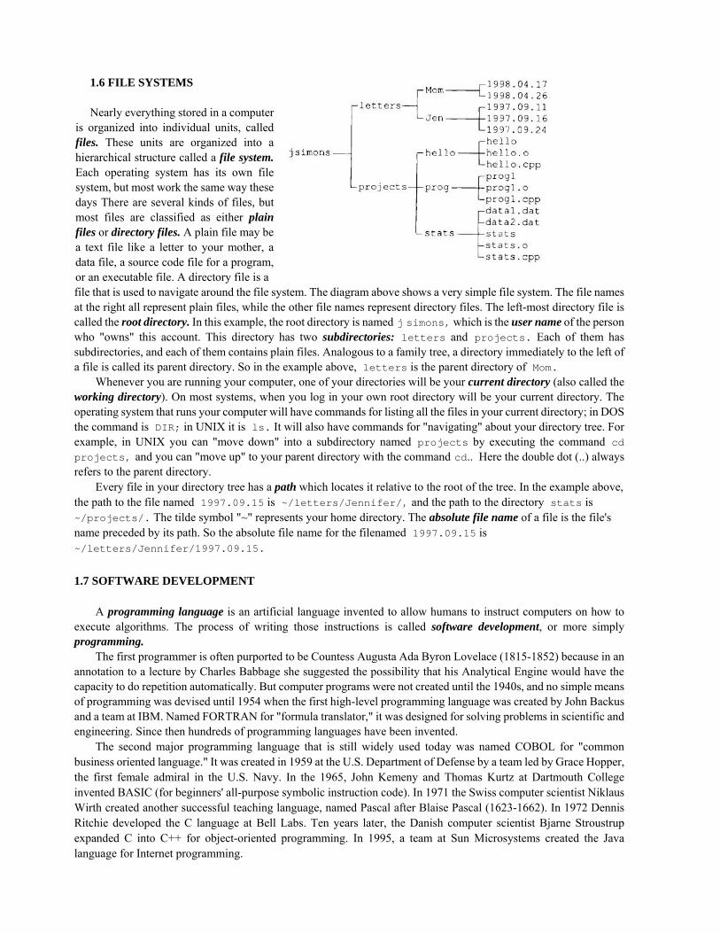
1.6 FILE SYSTEMS Nearly everything stored in a computer
is organized into individual units, called files. These units are organized into a hierarchical structure called a file system. Each operating system has its own file system, but most work the same way these days There are several kinds of files, but most files are classified as either plain files or directory files. A plain file may be a text file like a letter to your mother, a data file, a source code file for a program, or an executable file. A directory file is a
file that is used to navigate around the file system. The diagram above shows a very simple file system. The file names at the right all represent plain files, while the other file names represent directory files. The left-most directory file is called the root directory. In this example, the root directory is named j simons, which is the user name of the person who "owns" this account. This directory has two subdirectories: letters and projects. Each of them has subdirectories, and each of them contains plain files. Analogous to a family tree, a directory immediately to the left of a file is called its parent directory. So in the example above, letters is the parent directory of Mom.
Whenever you are running your computer, one of your directories will be your current directory (also called the working directory). On most systems, when you log in your own root directory will be your current directory. The operating system that runs your computer will have commands for listing all the files in your current directory; in DOS the command is DIR; in UNIX it is ls. It will also have commands for "navigating" about your directory tree. For example, in UNIX you can "move down" into a subdirectory named projects by executing the command cd projects, and you can "move up" to your parent directory with the command cd.. Here the double dot (..) always refers to the parent directory.
Every file in your directory tree has a path which locates it relative to the root of the tree. In the example above, the path to the file named 1997.09.15 is ~/letters/Jennifer/, and the path to the directory stats is ~/projects/. The tilde symbol "~" represents your home directory. The absolute file name of a file is the file's name preceded by its path. So the absolute file name for the filenamed 1997.09.15 is ~/letters/Jennifer/1997.09.15.
1.7 SOFTWARE DEVELOPMENT
A programming language is an artificial language invented to allow humans to instruct computers on how to execute algorithms. The process of writing those instructions is called software development, or more simply programming.
The first programmer is often purported to be Countess Augusta Ada Byron Lovelace (1815-1852) because in an annotation to a lecture by Charles Babbage she suggested the possibility that his Analytical Engine would have the capacity to do repetition automatically. But computer programs were not created until the 1940s, and no simple means of programming was devised until 1954 when the first high-level programming language was created by John Backus and a team at IBM. Named FORTRAN for "formula translator," it was designed for solving problems in scientific and engineering. Since then hundreds of programming languages have been invented.
The second major programming language that is still widely used today was named COBOL for "common business oriented language." It was created in 1959 at the U.S. Department of Defense by a team led by Grace Hopper, the first female admiral in the U.S. Navy. In the 1965, John Kemeny and Thomas Kurtz at Dartmouth College invented BASIC (for beginners' all-purpose symbolic instruction code). In 1971 the Swiss computer scientist Niklaus Wirth created another successful teaching language, named Pascal after Blaise Pascal (1623-1662). In 1972 Dennis Ritchie developed the C language at Bell Labs. Ten years later, the Danish computer scientist Bjarne Stroustrup expanded C into C++ for object-oriented programming. In 1995, a team at Sun Microsystems created the Java language for Internet programming.
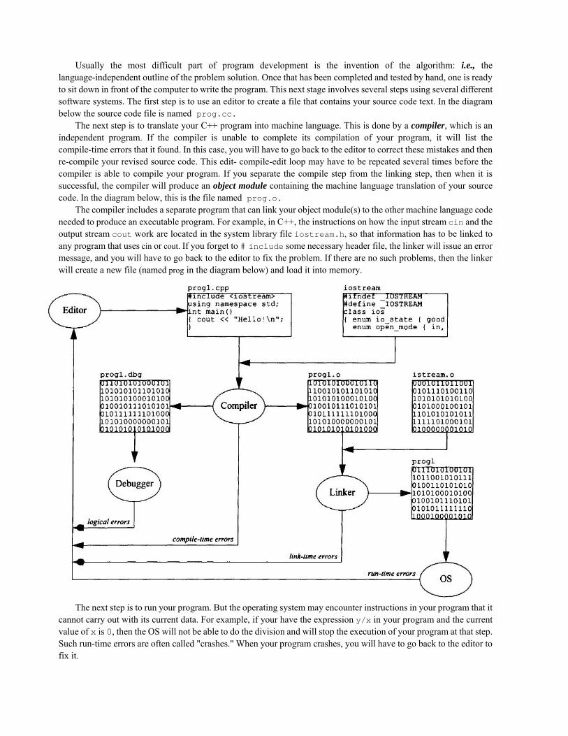
Usually the most difficult part of program development is the invention of the algorithm: i.e., the language-independent outline of the problem solution. Once that has been completed and tested by hand, one is ready to sit down in front of the computer to write the program. This next stage involves several steps using several different software systems. The first step is to use an editor to create a file that contains your source code text. In the diagram below the source code file is named prog.cc.
The next step is to translate your C++ program into machine language. This is done by a compiler, which is an independent program. If the compiler is unable to complete its compilation of your program, it will list the compile-time errors that it found. In this case, you will have to go back to the editor to correct these mistakes and then re-compile your revised source code. This edit- compile-edit loop may have to be repeated several times before the compiler is able to compile your program. If you separate the compile step from the linking step, then when it is successful, the compiler will produce an object module containing the machine language translation of your source code. In the diagram below, this is the file named prog.o.
The compiler includes a separate program that can link your object module(s) to the other machine language code needed to produce an executable program. For example, in C++, the instructions on how the input stream cin and the output stream cout work are located in the system library file iostream.h, so that information has to be linked to any program that uses cin or cout. If you forget to # include some necessary header file, the linker will issue an error message, and you will have to go back to the editor to fix the problem. If there are no such problems, then the linker will create a new file (named prog in the diagram below) and load it into memory.
The next step is to run your program. But the operating system may encounter instructions in your program that it cannot carry out with its current data. For example, if your have the expression y/x in your program and the current value of x is 0, then the OS will not be able to do the division and will stop the execution of your program at that step. Such run-time errors are often called "crashes." When your program crashes, you will have to go back to the editor to fix it.
Finally, once your program is running, the last step is to test it with various input sets. If it does not run correctly, you will have to return again to the editor to fix your logical errors. These are the most troublesome errors because none of the development systems (the compile, the linker/loader, the OS) is able to find them for you. It's up to you do a logical re-analysis of your algorithm to find the problem. With large programs, this task can be very difficult. Fortunately, most compilers come equipped with a debugger that can help you with this task. A debugger allows you to trace through your program step-by-step so you can see its logic. It also allows you to check the values of your variables at each step so you can see the details of the execution.
Compile-time errors are reduced by learning the requirements of the programming language. This comes mostly through experience, although a good IDE (Integrated Development Environment) with color-coded syntax can help here. Link-time errors are due mostly to repeated or absent definitions when a multi-file program is linked. These can be reduced by testing the independent modules before they are linked together. Run-time errors are usually caused by careless use of operators. Programming experience and knowledge of operator limitations can help reduce these errors. Logical errors are caused my many mistakes, such as poor planning and careless hacking. Efficient use of a debugger is the best way to solve those problems.
Correcting run-time errors and logical errors may require some major revisions to your program, which might generate more compile-time errors. In general, the program development process can lead to retracing many of the inner correction cycles, as shown in the picture.
Obviously, the programmer wants to minimize the number of times these cycles have to be repeated. Many modern compilers are part of a larger Integrated Development Environment (IDE) that helps the programmer reduce the number of cycles repeated. A good IDE integrates the compiler with the editor and the debugger so that they work together. For example, when the compiler locates a syntax error it will automatically re-launch the editor with the program in it and the cursor placed at the point where the error occurs. Some IDEs also include class inspectors, library inspectors, and other visual aids that help the programmer see the structure of his/her programs more clearly.
Review Questions
1.1 Match the names on the left with achievements on the right. Aiken, Howard H.
Babbage, Charles Backus, John Eckert, J. Presper Hollerith, Herman Jacquard, Joseph Marie Leibniz, Gottfried Wilhelm Mauchly, John W. Pascal, Blaise Schickard, Wilhelm Stroustrup, Bjarne von Neumann, John
marketed the first calculator built the first mechanical calculator built the first successful automatic calculator Created the first stored program designed the first programmable computer built the first commercially successful data processor built the first successful electromechanical computer jointly built the first electronic digital computer jointly built the first electronic digital computer designed the prototype of the modern computer created FORTRAN, the first programming language created the C++ programming language
1.2 Match the acronyms on the left with the descriptions on the right: ASCII the modern computer design created by John von Neumann in 1945 CD a small computer usually owned by a single person independently COBOL secondary storage that cannot be changed CPU memory or disk space for 210 bytes; about 1,000 bytes ENIAC the main memory in a computer FORTRAN a small optical disk used for secondary storage GB the first company to sell computers, founded by Eckert and Mauchly in 1949 IAS a removable memory module; typical sizes: 1 MB, 4 MB, 16 MB, 64 MB IDE the original programming language designed for business applications
KB units of speed for a computer clock: 1,000,000 cycles/second MB a software systems that integrates an editor, a compiler, and a debugger MHz the "brain" of a computer OS memory or disk space for 220 bytes; about 1,000,000 bytes PC memory or disk space for 230 bytes; about 1,000,000,000 bytes RAM memory or disk space for 240 bytes; about 1,000,000,000,000 bytes ROM the program that controls all operations of a computer SIMM the first high-level programming language, used mostly by scientists TB the huge computer built by Eckert and Mauchly in 1945 UNIVAC the code used by most computer systems to translate characters into integers
1.3 Describe the basic components of a computer.
1.4 What various kinds of memory units are found in modern computers?
1.5 How is memory organized in a computer?
1.6 What happens when you "boot" a computer?
1.7 What is an operating system? 1.8 What is a file system? 1.9 What is a file path name?
1.10 What is a computer program?
1.11 How is a computer program executed?
1.12 What kinds of errors typically occur in the programming process? 1.13 What is the fundamental distinction between integers and real numbers in a computer?
Problems
1.14 In a PC with 16 MB of RAM, how many actual bytes would memory hold and what would be the last address? 1.15 In a PC with 1 GB of RAM, how many actual bytes would memory hold and what would be the last address? 1.16 Charles Babbage (see page 2) won the first government research grant in history when in 1823 he persuaded the
British government to finance the construction of his Difference Engine. In his proposal to the government he used 41 as an example of a mathematical function that the computer would tabulate by means of the Method of Finite Differences. Construct a difference table for this function and explain how it facilitates its evaluation.
1.17 Use the method of Finite Differences to tabulate the function x 3x 5.
1.18 Use the method of Finite Differences to tabulate the function x 3x 5.
1.19 Explain why the Babylonian Algorithm (Algorithm 1.1) works. 1.20 The Babylonain Algorithm (Algorithm 1.1) can be modified easily to compute the square root of any positive
number: just change the 2 in Step 2 to the number whose square root you want. For example, to compute the square root of six (√6), do this for Step 2: 2. Replace x with the average of x and 6/x. a. Use a modified Babylonian Algorithm to compute √6. b. Use a modified Babylonian Algorithm to compute √666. c. Use a modified Babylonian Algorithm to compute √0.0066. Be sure to check your answers by squaring them.
1.21 Determine empirically how many iterations are needed for the Babylonian Algorithm to compute √25 to: a. 3 decimal place accuracy; b. 6 decimal place accuracy; c. 9 decimal place accuracy; d. 12 decimal place accuracy.
1.22 Determine what 4 one-byte integers are stored in these 4 bytes:1.23 Determine what 2 two-byte integers are stored in the 4 bytes shown
⋮
in Problem 1.22. 1.24 Determine what four-byte integer is stored in the 4 bytes of memory shown in
Problem 1.22. 1.25 Convert 110111002 to decimal. (Use Algorithm 1.2 on page 5.)
00100010
01100001
00010001
00000000
⋮
1.26 Convert each of the following binary numerals to decimal: a. 11011110 b. 10101010 c. 11111111
d. 10000000000000000000000000000000 (31 zeros)
1.27 Convert 55510 to binary.
1.28 Convert each of the following decimal numerals to binary: a. 888 b. 4444 c. 1025 d. 255
1.29 A hexadecimal numeral uses base 16. This requires the use of 16 symbols ("digits"). We use the 10 ordinary digits plus the first 6 letters of the alphabet. For example, the hexadecimal numeral 9ca2f represents 9 ⋅ 16 12 ⋅ 16 10 ⋅ 16 2 ⋅ 16 15 ⋅ 16 641,58310 . Devise an algorithm similar to that in Algorithm 1.4 to convert decimal to hexadecimal, and then apply it to find the hexadecimal representation for 100,00010.
1.30 Convert each of the decimal numbers in Problem 1.28 to hexadecimal (see Problem 1.29): 1.31 Convert the hexadecimal 2d7b into decimal.
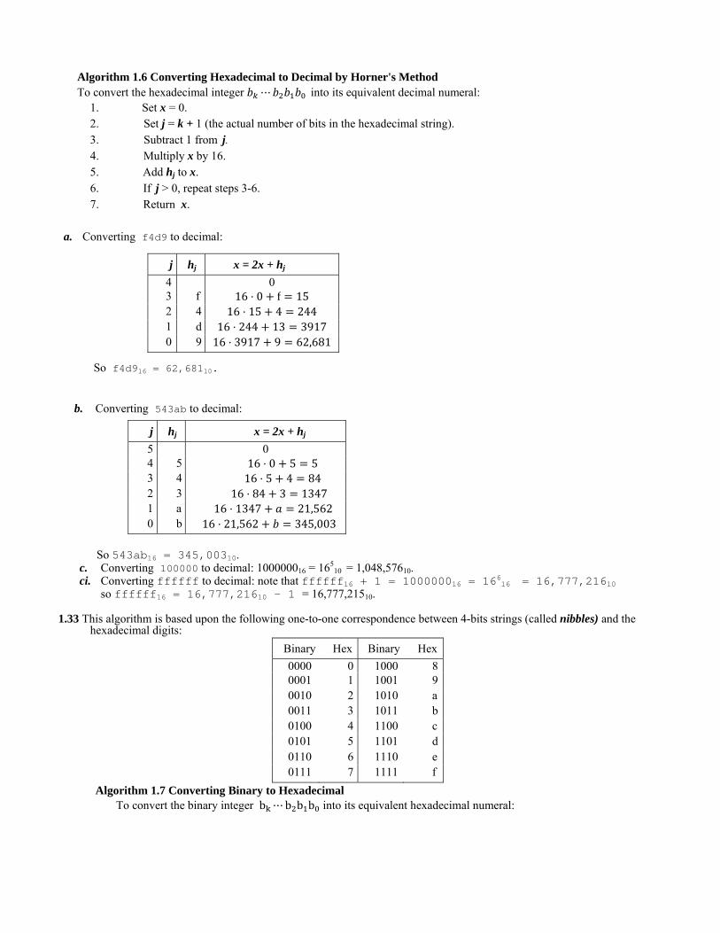
1.32 Create an algorithm that uses Horner's Method to convert hexadecimal to decimal, reversing Algorithm 1.4 on page 6. The algorithm should be similar to Algorithm 1.2 on page 5. Use it to convert each of the following hexadecimal numerals (see Problem 1.29) to decimal: a. f4d9 b. 543ab c. 100000 d. ffffff
1.33 Create an algorithm to convert binary to hexadecimal, and then apply it to find the hexadecimal representation for each of the numerals in Problem 1.26.
1.34 Horner's Method (page 5) is more efficient than the usual method for evaluating a polynomial. For example, the polynomial 2 7 6x 9x 8 5 can be written as
2 7 6 9 8 5 Then a value such 4.1 can be computed as 4.1 2 ⋅ 4.1 7 ⋅ 4.1 6 ⋅ 4.1 9 ⋅ 4.1 8 ⋅ 4.1 5
1.2 ⋅ 4.1 6 ⋅ 4.1 9 ⋅ 4.1 8 ⋅ 4.1 510.92 ⋅ 4.1 9 ⋅ 4.1 8 ⋅ 4.1 553.772 ⋅ 4.1 8 ⋅ 4.1 5931.70732
The advantage of Horner's Method is that it eliminates exponentiation. Use Horner's Method to evaluate 3.4 for this polynomial.
1.35 Use Horner's Method to evaluate 3.4 for 3 5 2x x 8 6.
1.36 Use Horner's Method to evaluate 3.4 for 3 2 4x 5 .
1.37 Consider the general nth degree polynomial ⋯ a x . Compare the number of multiplications that it takes to evaluate this directly (using exponentiation) with the number of multiplications required by Horner's Method.
Solutions
1.1 Howard H. Aiken built the first successful electromechanical computer; Charles Babbage designed the first programmable computer;
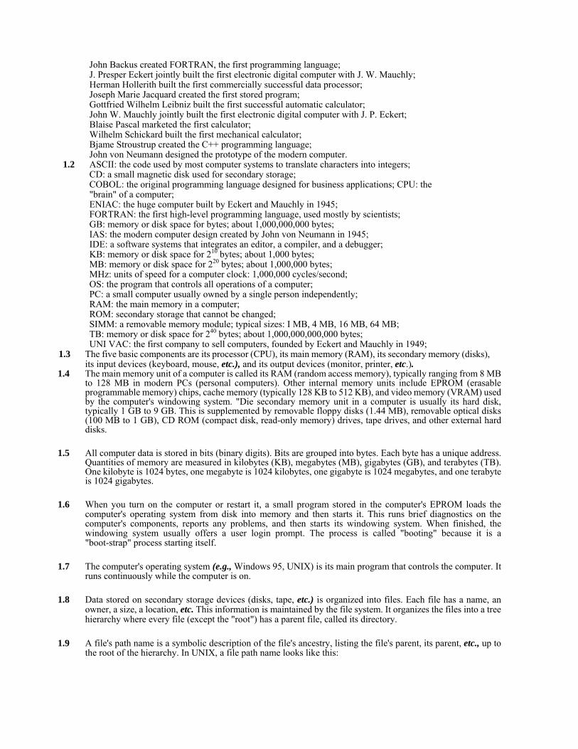
John Backus created FORTRAN, the first programming language; J. Presper Eckert jointly built the first electronic digital computer with J. W. Mauchly; Herman Hollerith built the first commercially successful data processor; Joseph Marie Jacquard created the first stored program; Gottfried Wilhelm Leibniz built the first successful automatic calculator; John W. Mauchly jointly built the first electronic digital computer with J. P. Eckert; Blaise Pascal marketed the first calculator; Wilhelm Schickard built the first mechanical calculator; Bjame Stroustrup created the C++ programming language; John von Neumann designed the prototype of the modern computer.
1.2 ASCII: the code used by most computer systems to translate characters into integers; CD: a small magnetic disk used for secondary storage; COBOL: the original programming language designed for business applications; CPU: the "brain" of a computer; ENIAC: the huge computer built by Eckert and Mauchly in 1945; FORTRAN: the first high-level programming language, used mostly by scientists; GB: memory or disk space for bytes; about 1,000,000,000 bytes; IAS: the modern computer design created by John von Neumann in 1945; IDE: a software systems that integrates an editor, a compiler, and a debugger; KB: memory or disk space for 210 bytes; about 1,000 bytes; MB: memory or disk space for 220 bytes; about 1,000,000 bytes; MHz: units of speed for a computer clock: 1,000,000 cycles/second; OS: the program that controls all operations of a computer; PC: a small computer usually owned by a single person independently; RAM: the main memory in a computer; ROM: secondary storage that cannot be changed; SIMM: a removable memory module; typical sizes: I MB, 4 MB, 16 MB, 64 MB; TB: memory or disk space for 240 bytes; about 1,000,000,000,000 bytes; UNI VAC: the first company to sell computers, founded by Eckert and Mauchly in 1949;
1.3 The five basic components are its processor (CPU), its main memory (RAM), its secondary memory (disks), its input devices (keyboard, mouse, etc.), and its output devices (monitor, printer, etc.).
1.4 The main memory unit of a computer is called its RAM (random access memory), typically ranging from 8 MB to 128 MB in modern PCs (personal computers). Other internal memory units include EPROM (erasable programmable memory) chips, cache memory (typically 128 KB to 512 KB), and video memory (VRAM) used by the computer's windowing system. "Die secondary memory unit in a computer is usually its hard disk, typically 1 GB to 9 GB. This is supplemented by removable floppy disks (1.44 MB), removable optical disks (100 MB to 1 GB), CD ROM (compact disk, read-only memory) drives, tape drives, and other external hard disks.
1.5 All computer data is stored in bits (binary digits). Bits are grouped into bytes. Each byte has a unique address. Quantities of memory are measured in kilobytes (KB), megabytes (MB), gigabytes (GB), and terabytes (TB). One kilobyte is 1024 bytes, one megabyte is 1024 kilobytes, one gigabyte is 1024 megabytes, and one terabyte is 1024 gigabytes.
1.6 When you turn on the computer or restart it, a small program stored in the computer's EPROM loads the computer's operating system from disk into memory and then starts it. This runs brief diagnostics on the computer's components, reports any problems, and then starts its windowing system. When finished, the windowing system usually offers a user login prompt. The process is called "booting" because it is a "boot-strap" process starting itself.
1.7 The computer's operating system (e.g., Windows 95, UNIX) is its main program that controls the computer. It runs continuously while the computer is on.
1.8 Data stored on secondary storage devices (disks, tape, etc.) is organized into files. Each file has a name, an owner, a size, a location, etc. This information is maintained by the file system. It organizes the files into a tree hierarchy where every file (except the "root") has a parent file, called its directory.
1.9 A file's path name is a symbolic description of the file's ancestry, listing the file's parent, its parent, etc., up to the root of the hierarchy. In UNIX, a file path name looks like this:
/Users/j smith/cslOl/projects/Hello.cc Each directory is denoted by the
directory's name ending with the slash character ' / '. 1.10 A computer program is a file containing instructions for the computer to carry out an algorithm. When the
program is run, the computer carries out (executes) its instructions.
1.11 Most computer programs are written in high level programming languages such as C++ or Java. The file containing this source code is then compiled into the equivalent machine language program stored in a separate file. In UNIX, the program is then run by using the name of its executable file as a command.
1.12 The three main kinds of errors are compile-time errors, run-time errors, and logical errors. Compile- time errors are detected and reported by the compiler when the programmer attempts to compile the program. Run-time errors can be detected and reported by the operating system when the programmer attempts to run the program. Logical errors must be detected by the programmer by means of testing the program on various input sets.
1.13 Integers are exact; real numbers are only approximate.
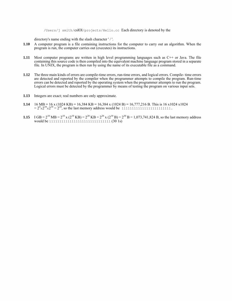
1.14 16 MB = 16 x (1024 KB) = 16,384 KB = 16,384 x (1024 B) = 16,777,216 B. This is 16 x1024 x1024 = 24x210x210 = 224, so the last memory address would be 111111111111111111111111.
1.15 I GB = 210 MB = 210 x (210 KB) = 220 KB = 220 x (210 B) = 230 B = 1,073,741,824 B, so the last memory address would be 111111111111111111111111111111 (30 1s)
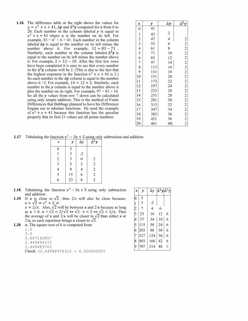
1.16 The difference table at the right shows the values for
41, ∆ and ∆ computed for x from 0 to 20. Each number in the column labeled y is equal to
41 where x is the number on its left. For example, 83 = 62 + 6 + 41. Each number in the column labeled ∆ is equal to the number on its left minus the number above it. For example, 12 83 71 . Similarly, each number in the column labeled ∆ is equal to the number on its left minus the number above it. For example, 2 12 10. After the first few rows have been completed it is easy to see that every number in the ∆ column will be 2. (This is due to the fact that the highest exponent in the function 41 is 2.) So each number in the ∆ column is equal to the number above it +2. For example, 14 12 2. Similarly, each number in the y column is equal to the number above it plus the number on its right. For example, 97 = 83 + 14. So all the y values from row 7 down can be calculated using only simple addition. This is the method of Finite Differences that Babbage planned to have his Difference Engine use to tabulate functions. He used the example of 41 because this function has the peculiar property that its first 21 values are all prime numbers
x y ∆ ∆ 0 1
41
43
2
2 47 4 2 3 53 6 2 4 61 8 2 5 71 10 2 6 83 12 2 7 97 14 2 8 113 16 2 9 131 18 2
10 151 20 2 11 173 22 2 12 197 24 2 13 223 26 2 14 251 28 2 15 281 30 2 16 313 32 2 17 347 34 2 18 383 36 2 19 421 38 2 20 461 40| 2
1.17 Tabulating the function x 3x 5 using only subtraction and addition: x y ∆y ∆
0 5
1 3 -2
2 3 0 2 3 5 2 2 4 9 4 2 5 15 6 2 6 23 8 2
1.18 Tabulating the function x 3x 5 using only subtraction
and addition: 1.19 If x is close to √2 , then 2/x will also be close because:
x √2 ⇒ 2 ⇒2/ . Also, √2 will be between x and 2/x because as long
as x > 0, x < √2 2/√2 ⇔ √2 ⋅ 2 ⇔ √2 2/ . Thus the average of x and 2/x will be closer to √2 than either x or 2/x, so each repetition brings x closer to √2.
1.20 a. The square root of 6 is computed from 1.0 3.5 2.607142857 2.449494372 2.449489743 Check: (2.449489743)2 = 6.000000001
x y ∆y ∆ ∆ y
0 1
5 3 -2
2 7 4 6
3 23 16 12 6 4 57 34 18 6 5 115 58 24 6 6 203 88 30 6 7 327 124 36 6 8 493 166 42 6 9 707 214 48 6
333.5 The square root of 666 is computed from 1.0
b. 167.7485007 85.85936499 46.80811789 30.51820954 26.17062301 25.80950228 25.80697592 25.80697580 Check: (25.80697580)2 = 665.9999999
c. The square root of 0.0066 is computed from 1.0
0.5033 0.258206726 0.141883820 0.094200376 0.082131895 0.081245223 0.081240384
Check: (0.081240384)2 = 0.006599999 1.21 a. It takes 5 iterations to obtain 3 decimal place accuracy for √25.
b. It takes 6 iterations to obtain 6 decimal place accuracy for √25. c. It takes 6 iterations to obtain 9 decimal place accuracy for √25. d. It takes 7 iterations to obtain 12 decimal place accuracy for √25.
1.22 001000102 = 25 + 21 = 32 + 2 = 34. 011000012 = 26 + 25 + 20 = 64 + 32 +1 = 97. 000100012 = 24 + 20 = 16 + 1 = 17. 000000002 = 0.
1.23 01100001001000102 = 214 + 213 + 28 + 25 + 21 = 16,384 + 8192 + 256 + 32 + 2 = 24,866. Note that this result can also be computed from the answers to Problem 1.22: 97 ⋅ 2 34 97 ⋅ 256 34 24,866. 00000000000100012 = 24 + 2° = 16 + 1 = 17.
1.24 000000000001000101100001001000102 = 220 + 216 + 214 + 213 + 28 + 25 + 21 = 1,048,576 + 65,536 + 16,384 + 8192 + 256 + 32 + 2 = 1,138,978. Note that this result can also be computed from the answers to Problem 1.23: 2 ⋅ 17 24,866 65536 ⋅ 17 24,866 1114112 24,866 1,138,978.
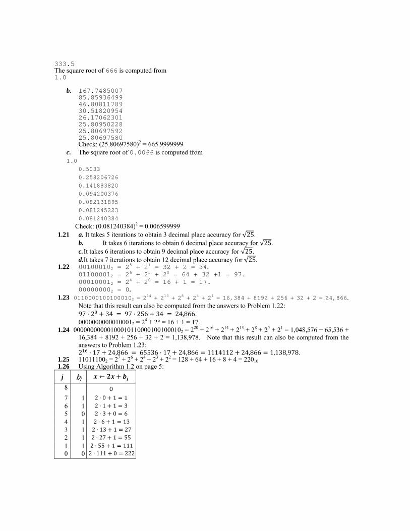
1.25 110111002 = 27 + 26 + 24 + 23 + 22 = 128 + 64 + 16 + 8 + 4 = 22010 1.26 Using Algorithm 1.2 on page 5:
j bj ←
8 0 7 1 2 ⋅ 0 1 1
6 1 2 ⋅ 1 1 3 5 0 2 ⋅ 3 0 6
4 1 2 ⋅ 6 1 13 3 1 2 ⋅ 13 1 27 2 1 2 ⋅ 27 1 55
1 1 2 ⋅ 55 1 111 0 0 2 ⋅ 111 0 222
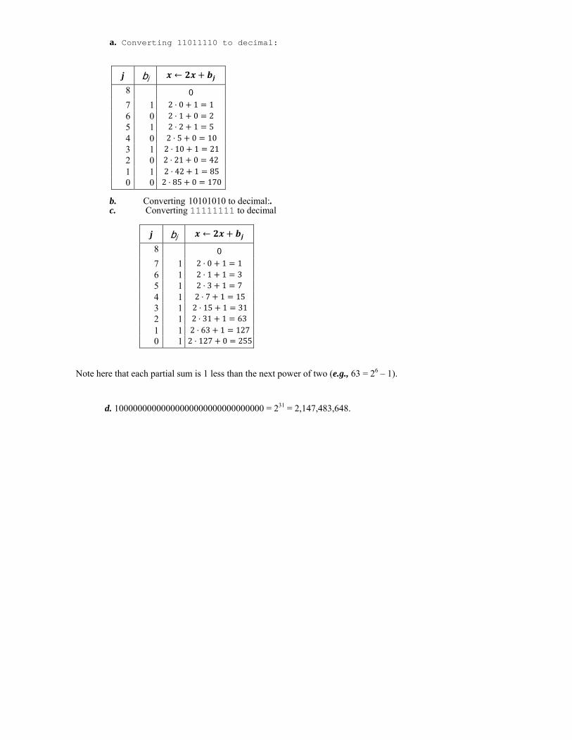
a. Converting 11011110 to decimal: b. Converting 10101010 to decimal:. c. Converting 11111111 to decimal
j bj ←
8 0 7 1 2 ⋅ 0 1 1
6 1 2 ⋅ 1 1 3 5 1 2 ⋅ 3 1 7
4 1 2 ⋅ 7 1 15 3 1 2 ⋅ 15 1 31 2 1 2 ⋅ 31 1 63
1 1 2 ⋅ 63 1 1270 1 2 ⋅ 127 0 255
Note here that each partial sum is 1 less than the next power of two (e.g., 63 = 26 – 1).
d. 10000000000000000000000000000000 = 231 = 2,147,483,648.
j bj ←
8 0 7 1 2 ⋅ 0 1 1
6 0 2 ⋅ 1 0 2 5 1 2 ⋅ 2 1 5
4 0 2 ⋅ 5 0 10 3 1 2 ⋅ 10 1 21 2 0 2 ⋅ 21 0 42
1 1 2 ⋅ 42 1 85 0 0 2 ⋅ 85 0 170
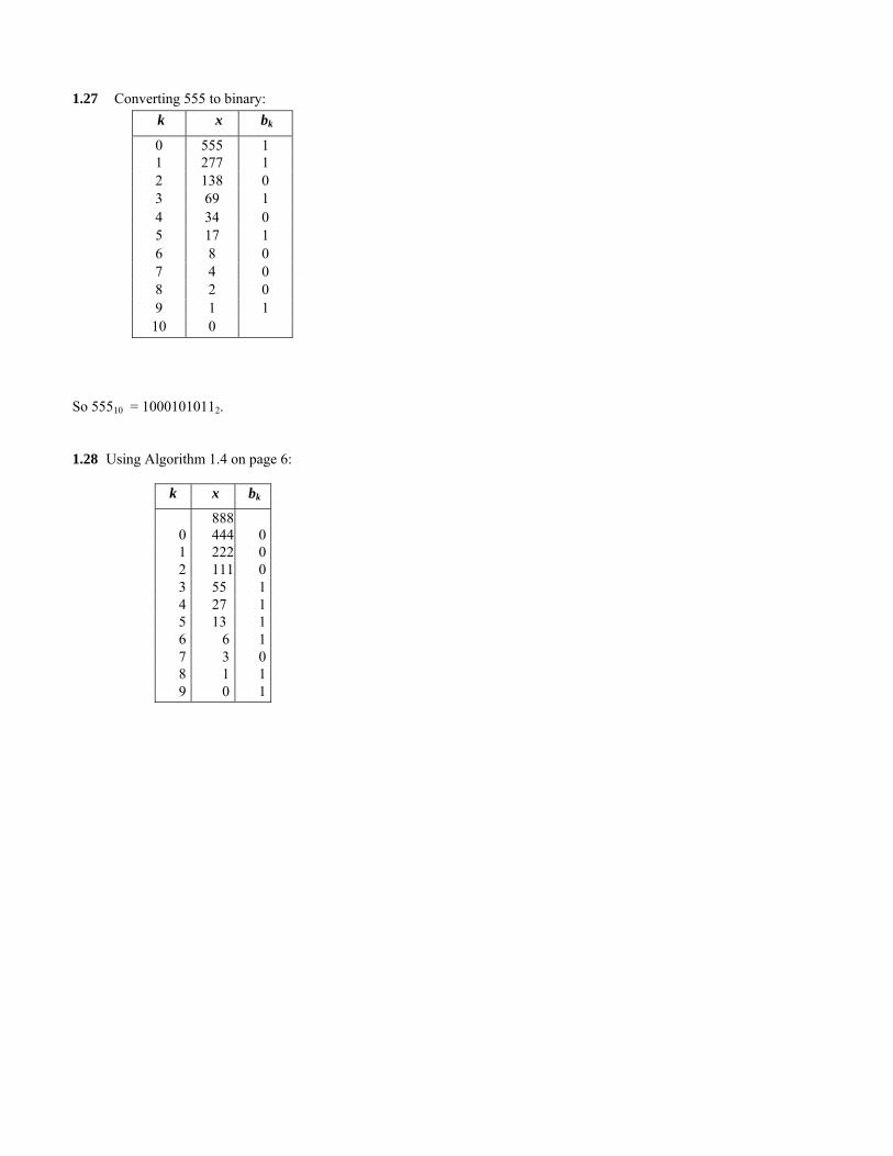
1.27 Converting 555 to binary:
So 55510 = 10001010112.
1.28 Using Algorithm 1.4 on page 6:
k x bk
0 555 1 1 277 1 2 138 0 3 69 1 4 34 0 5 17 1 6 8 0 7 4 0 8 2 0 9 1 1
10 0
k x bk
888
0 444 0 1 222 0 2 111 0 3 55 1 4 27 1 5 13 1 6 6 1 7 3 0 8 1 1 9 0 1
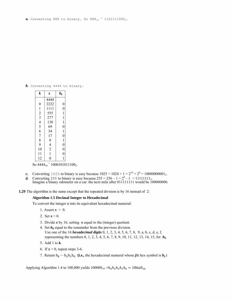
a. Converting 888 to binary. So 88810 = 11011110002. b. Converting 4444 to binary.
So 444410
= 10001010111002.
c. Converting 1025 to binary is easy because 1025 = 1024 + 1 = 210 + 20 = 100000000012. d. Converting 255 to binary is easy because 255 = 256 – 1 = 28 – 1 = 111111112.
Imagine a binary odometer on a car: the next mile after 011111111 would be 100000000.
1.29 The algorithm is the same except that the repeated division is by 16 instead of 2:
Algorithm 1.5 Decimal Integer to Hexadecimal
To convert the integer x into its equivalent hexadecimal numeral:
1. Assert x > 0.
2. Set x = 0.
3. Divide x by 16, setting x equal to the (integer) quotient. 4. Set hk equal to the remainder from the previous division. Use one of the 16 hexadecimal digits 0, 1, 2, 3, 4, 5, 6, 7, 8, 9, a, b, c, d, e, f, representing the numbers 0, 1, 2, 3, 4, 5, 6, 7, 8, 9, 10, 11, 12, 13, 14, 15, for hk.
5. Add 1 to k.
6. If x > 0, repeat steps 3-6.
7. Return h ⋯h h h {i.e., the hexadecimal numeral whose jth hex symbol is hj.)
Applying Algorithm 1.4 to 100,000 yields 1000001O = 186 0
k x bk
4444
0 2222 0 1 1111 0 2 555 1 3 277 1 4 138 1 5 69 0 6 34 1 7 17 0 8 8 1 9 4 0
10 2 0 11 1 0 12 0 1
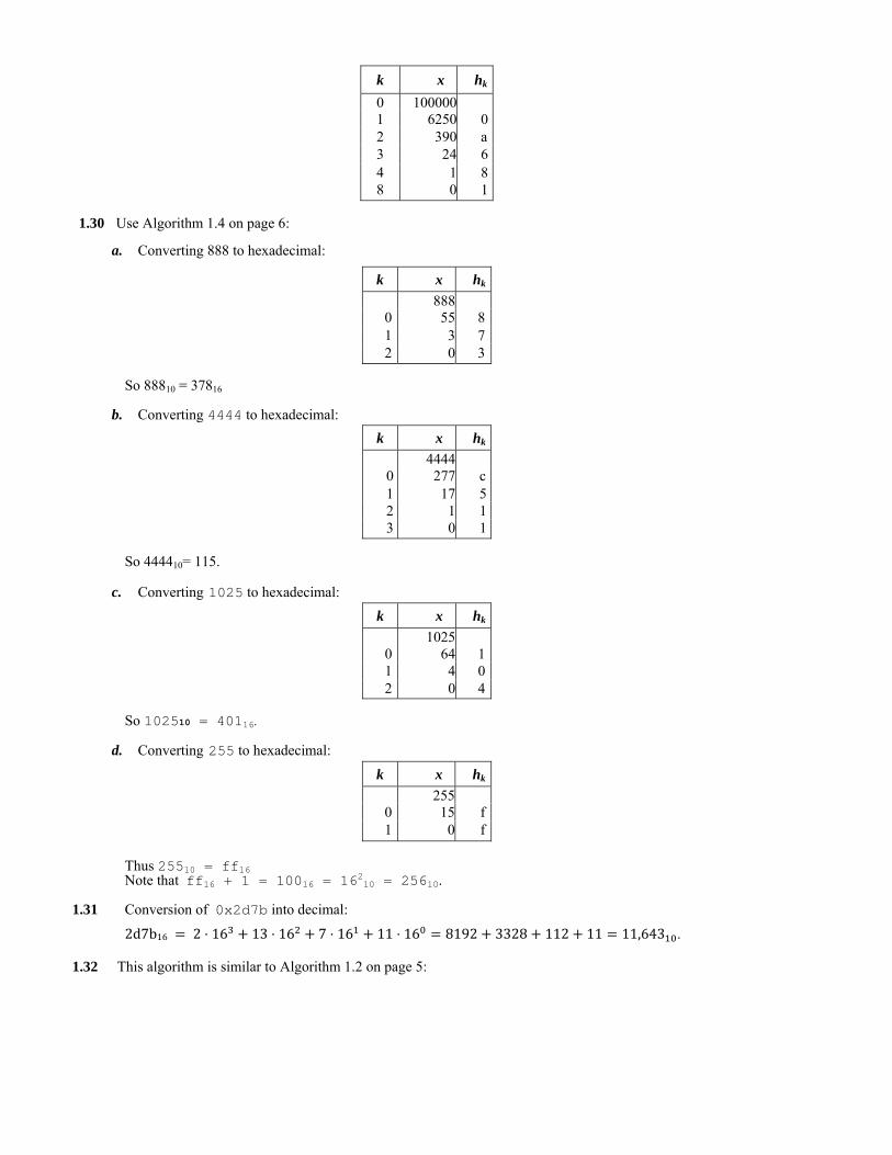
1.30 Use Algorithm 1.4 on page 6:
a. Converting 888 to hexadecimal:
So 88810 = 37816
b. Converting 4444 to hexadecimal:
So 444410= 115.
c. Converting 1025 to hexadecimal:
So 102510 = 40116.
d. Converting 255 to hexadecimal:
Thus 25510 = ff16 Note that ff16 + 1 = 10016 = 16210 = 25610.
1.31 Conversion of 0x2d7b into decimal:
2d7b16 2 ⋅ 16 13 ⋅ 16 7 ⋅ 16 11 ⋅ 16 8192 3328 112 11 11,643 .
1.32 This algorithm is similar to Algorithm 1.2 on page 5:
k x hk
0 100000
1 6250 02 390 a3 24 64 1 88 0 1
k x hk
888
0 55 81 3 72 0 3
k x hk
4444
0 277 c1 17 52 1 13 0 1
k x hk
1025
0 64 11 4 02 0 4
k x hk
255
0 15 f1 0 f
Algorithm 1.6 Converting Hexadecimal to Decimal by Horner's Method To convert the hexadecimal integer ⋯ into its equivalent decimal numeral:
1. Set x = 0. 2. Set j = k + 1 (the actual number of bits in the hexadecimal string). 3. Subtract 1 from j. 4. Multiply x by 16. 5. Add hj to x. 6. If j > 0, repeat steps 3-6. 7. Return x.
a. Converting f4d9 to decimal:
So f4d916 = 62,68110.
b. Converting 543ab to decimal:
So 543ab16 = 345,00310.
c. Converting 100000 to decimal: 100000016 = 16510 = 1,048,57610.
ci. Converting ffffff to decimal: note that ffffff16 + 1 = 100000016 = 16616 = 16,777,21610 so ffffff16 = 16,777,21610 - 1 = 16,777,21510.
1.33 This algorithm is based upon the following one-to-one correspondence between 4-bits strings (called nibbles) and the
hexadecimal digits:
Algorithm 1.7 Converting Binary to Hexadecimal To convert the binary integer b ⋯b b b into its equivalent hexadecimal numeral:
j hj x = 2x + hj
4 0 3 f 16 ⋅ 0 f 15 2 4 16 ⋅ 15 4 244 1 d 16 ⋅ 244 13 3917 0 9 16 ⋅ 3917 9 62,681
j hj x = 2x + hj
5 0 4 5 16 ⋅ 0 5 5 3 4 16 ⋅ 5 4 84 2 3 16 ⋅ 84 3 1347 1 a 16 ⋅ 1347 21,562 0 b 16 ⋅ 21,562 345,003
Binary Hex Binary Hex
0000 0 1000 80001 1 1001 90010 2 1010 a0011 3 1011 b0100 4 1100 c0101 5 1101 d0110 6 1110 e0111 7 1111 f
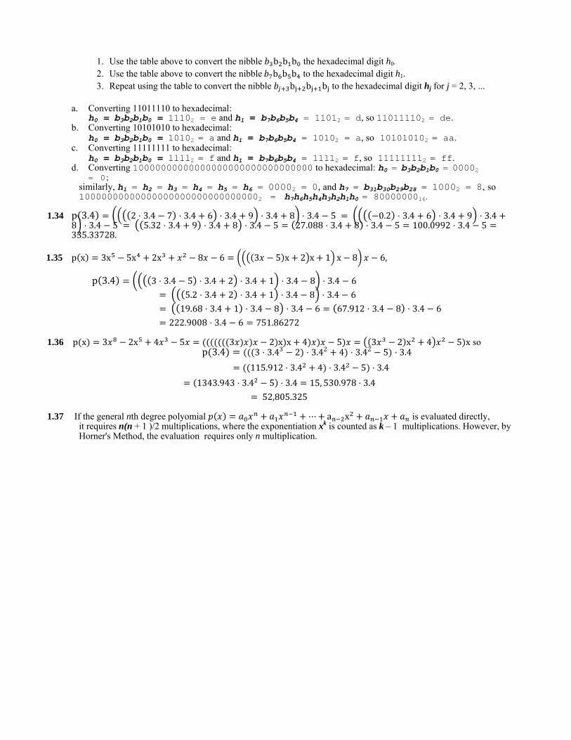
1. Use the table above to convert the nibble b b b the hexadecimal digit h0. 2. Use the table above to convert the nibble b b b to the hexadecimal digit h1. 3. Repeat using the table to convert the nibble b b b to the hexadecimal digit hj for j = 2, 3, ...
a. Converting 11011110 to hexadecimal:
h0 = b3b2b1b0 = 11102 = e and h1 = b7b6b5b4 = 11012 = d, so 110111102 = de. b. Converting 10101010 to hexadecimal:
h0 = b3b2blb0 = 10102 = a and h1 = b7b6b5b4 = 10102 = a, so 101010102 = aa. c. Converting 11111111 to hexadecimal:
h0 = b3b2b1b0 = llll2 = f and h1 = b7b6b5b4 = 11112 = f, so 111111112 = ff. d. Converting 10000000000000000000000000000000 to hexadecimal: h0 = b3b2b1b0 = 00002
= 0 ; similarly, h1 = h2 = h3 = h4 = h5 = h6 = 00002 = 0, and h7 = b31b30b29b28 = 10002 = 8, so 100000000000000000000000000000002 = h7h6h5h4h3h2h1h0 = 8000000016.
1.34 p 3.4 2 ⋅ 3.4 7 ⋅ 3.4 6 ⋅ 3.4 9 ⋅ 3.4 8 ⋅ 3.4 5 0.2 ⋅ 3.4 6 ⋅ 3.4 9 ⋅ 3.48 ⋅ 3.4 5 5.32 ⋅ 3.4 9 ⋅ 3.4 8 ⋅ 3.4 5 27.088 ⋅ 3.4 8 ⋅ 3.4 5 100.0992 ⋅ 3.4 5335.33728.
1.35 p x 3x 5x 2x 8 6 3 5 x 2 x 1 x 8 6,
p 3.4 3 ⋅ 3.4 5 ⋅ 3.4 2 ⋅ 3.4 1 ⋅ 3.4 8 ⋅ 3.4 6
5.2 ⋅ 3.4 2 ⋅ 3.4 1 ⋅ 3.4 8 ⋅ 3.4 6
19.68 ⋅ 3.4 1 ⋅ 3.4 8 ⋅ 3.4 6 67.912 ⋅ 3.4 8 ⋅ 3.4 6
222.9008 ⋅ 3.4 6 751.86272
1.36 p x 3 2x 4 5 3 2 x x 4 5 3 2 x 4 5 x sop 3.4 3 ⋅ 3.43 2 ⋅ 3.42 4 ⋅ 3.42 5 ⋅ 3.4
115.912 ⋅ 3.4 4 ⋅ 3.4 5 ⋅ 3.4
1343.943 ⋅ 3.4 5 ⋅ 3.4 15, 530.978 ⋅ 3.4
52,805.325
1.37 If the general nth degree polyomial ⋯ a x is evaluated directly, it requires n(n + 1 )/2 multiplications, where the exponentiation xk is counted as k – 1 multiplications. However, by Horner's Method, the evaluation requires only n multiplication.