Embed Size (px)
Citation preview
Theories for Subexponential-size Bounded-depthFrege Proofs
Kaveh Ghasemloo and Stephen Cook
Department of Computer ScienceUniversity of Toronto
Canada
CSL 2013
1 / 19

2 / 19

Propositional vs Uniform Proof Complexity
Propositional proof complexity studies the lengths of proofs oftautology families in proof systems such as Frege and bdFrege(bounded-depth Frege).
Uniform proof complexity studies the power of weak formal theoriessuch as VNC1 and V0.
Both proof systems and theories are often associated with complexityclasses.
I Frege systems and VNC1 are associated with the complexity class NC1
I bdFrege and V0 are associated with the complexity class AC0.
3 / 19

Complexity Classes, Theories, and Proof Systems
A three-way connection 〈 C, VC, C-Frege 〉Complexity class C, theory VC, and proof system C-Frege
The provably total functions in VC are those in C
C-Frege is the strongest propositional proof system whose soundness isprovable in VC
The ΣB0 theorems of VC translate to a family {ϕn}n of propositional
tautologies which have polynomial size C-Frege proofs.Example: VNC1 proves the Pigeonhole Principle: “For all n, n + 1pigeons cannot be assigned to n holes with at most one pigeon perhole.”The corresponding tautologies {ϕn}n have polysize Frege proofs.
Examples
〈 NC1, VNC1, Frege 〉〈 AC0, V0, bdFrege 〉〈 P, VP, eFrege 〉
4 / 19

Motivatation for our paper
1 Theorem[FPS’12]: Frege proofs can be converted to bdFrege proofs ofsubexponential size.
2 That is, given 0 < ε < 1 and a family {ϕn}n of tautologies and afamily {πn}n of Frege proofs such that πn proves ϕn and has sizenO(1), there exists a family {π′n}n of Frege proofs such that π′n provesϕn and has size 2O(nε) and all cut formulas have depth O(1).
3 We want a uniform version of this.
4 i.e. we want a triple 〈Cε,VCε,Cε-Frege〉 where Cε-Frege is as in item2 above.
5 Note that bdFrege and Cε-Frege are proof classes rather than proofsystems.A Proof class associates families of proofs with families of formulas.
5 / 19

What is the triple 〈Cε,VCε,Cε-Frege〉 for subexponential bdFrege?
Here ε = 1/d where d > 1 is an integer.
Let Cε = AltTime(O(1),O(nε))(problems computable by uniform size 2O(nε) bounded-depth circuitfamilies).
NC1 ⊆ L ⊆ NL ⊆ Cε
What is the theory VCε.?(We want the provably total functions of VCε to be those in Cε.)
Major Obstacle: In general the provably total functions in a theory VCare closed under compostion. But the subexponential functions are notclosed under composition.
For example the composition of n 7→ 2n12 with n 7→ n2 is 2n.
We’ll get to this in a moment.
6 / 19

We follow the framework in [Cook-Nguyen ’10]
Program in Chapter 9
1 Presents a general method for associating atheory VC with a complexity classes C,including theories
V0 ⊆ VNC1 ⊆ VL ⊆ VNL ⊆ VP
for classes
AC0 ⊆ NC1 ⊆ L ⊆ NL ⊆ P
2 Theories have two sorts: Natural numbersx , y , z , ... and bit strings X ,Y ,Z , ....
3 Function symbols 0, 1, +, ·, | | (length)
4 Relation symbols =, ≤, and ∈(membership/bit).
7 / 19

Two-sorted relations and formulas
(Uniform)AC0 = FO = AltTime(O(1),O(lgn)) = DepthSize(O(1), nO(1)).
A relation R(~x , ~X ) is in AC0 as above, where number arguments ~x arepresented in unary.
ΣB0 is the class of formulas with no string quantifiers, and with all
number quantifers bounded.
ΣB0 Representation Theorem: A relation R(~x , ~X ) is in AC0 iff it is
represented by a ΣB0 formula ϕ(~x , ~X ).
ΣBi and ΠB
i are classes of bounded formulas with limits on alternationsof the string quantifiers.
∃BΦ consists of formulas starting with bounded existential stringquantifiers followed by a formula in Φ.
8 / 19

Introducing io-typed theories ioVC to limit composition
Introduce two types of variables: input type and output type
input type: a, b, c denote numbers, A,B,C denote strings.output type: x , y , z denote numbers, X ,Y ,Z denote strings.
For fast growing f , the arugments of f have input type and are small,while the value of f has output type and might be large.
For each 0 < ε < 1, the functions with growth rate 2O(nε) are closedunder composition with linear functions, so we allow linear terms to beinput type.
All terms (including input type terms) have output type.
Example input type term:
a + b + 1 + pd(c) + |A|+ |B|
(No output type variables allowed.)
9 / 19

Theory io2Basic: Axioms have output type variables
Table: io2Basic
B1 x + 1 6= 0B2 x + 1 = y + 1→ x = yB3 x + 0 = xB4 x + (y + 1) = (x + y) + 1B5 x ·0 = 0B6 x ·(y + 1) = x ·y + x
B7 x ≤ y ∧ y ≤ x → x = yB8 x ≤ x + yB9 0 ≤ xB10 x ≤ y ∨ y ≤ xB11 x ≤ y ↔ x < y + 1B12 pd(0) = 0 ∧ (x 6= 0→
pd(x) + 1 = x)
L y ∈ X → y < |X |
X = Y abbreviates (|X | = |Y | ∧ ∀x ≤ |X | x ∈ X ↔ x ∈ Y ).
10 / 19

Theory ioV0 for AC0
ioV0 extends io2Basic by adding the substring function X [y , z ] and thefollowing axioms:
x ∈ X [y , z ]↔ x < z ∧ y + x ∈ X
|X [y , z ]| = z
Ind: 0 ∈ X ,∀y < z (y ∈ X → y + 1 ∈ X )⇒ z ∈ X
ϕ-CA (Comprehension): ∃Y = z ∀x < z(
x ∈ Y ↔ ϕ(x ,~a, ~A))
where ϕ(x ,~a, ~A) is in ΣB0
oiConvnum: ∃b ≤ a b = min(a, x)
oiConvstr: ∃B = a B = X [y , a]
Theorem: The ∃BΣB0 definable functions in ioV0 coincide with the AC0
functions.
11 / 19

Theory ioV0 for AC0
ioV0 extends io2Basic by adding the substring function X [y , z ] and thefollowing axioms:
x ∈ X [y , z ]↔ x < z ∧ y + x ∈ X
|X [y , z ]| = z
Ind: 0 ∈ X , ∀y < z (y ∈ X → y + 1 ∈ X )⇒ z ∈ X
ϕ-CA (Comprehension): ∃Y = z ∀x < z(
x ∈ Y ↔ ϕ(x ,~a, ~A))
where ϕ(x ,~a, ~A) is in ΣB0
oiConvnum: ∃b ≤ a b = min(a, x)
oiConvstr: ∃B = a B = X [y , a]
Theorem: The ∃BΣB0 definable functions in ioV0 coincide with the AC0
functions.
11 / 19

Theory ioVNC1 = ioV0 + ΣB0 (MBBFE)-CA
ΣB0 (MBBFE)-CA is the following axiom schema:
∃Y = 2s ∃Z = 2s [∀x < 2s (x ∈ Z ↔ ϕ(x ,~a, ~A))∧“Y is the computation of Z ”]
where s has output type and ϕ ∈ ΣB0 and “Y is the computation of Z ”
stands for
∀z < s [z+s ∈ Y ↔ z ∈ Z ]∧[(z ∈ Z → (z ∈ Y ↔ 2z ∈ Y ∧ 2z + 1 ∈ Y ))∧
(z /∈ Z → (z ∈ Y ↔ 2z ∈ Y ∨ 2z + 1 ∈ Y ))]
We think of ϕ as specifying the bit graph of an AC0 function whose outputZ is as an instance of MBBFE: its first half specifies the gates of theformula and its second half specifies the inputs to the formula.
Theorem: The ∃BΣB0 definable functions of ioVNC1 are precisely the
NC1 functions.
12 / 19

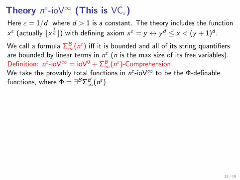
Theory nε-ioV∞ (This is VCε)
Here ε = 1/d , where d > 1 is a constant. The theory includes the function
xε (actually bx1d c) with defining axiom xε = y ↔ yd ≤ x < (y + 1)d .
We call a formula ΣB∞(nε) iff it is bounded and all of its string quantifiers
are bounded by linear terms in nε (n is the max size of its free variables).Definition: nε-ioV∞ = ioV0 + ΣB
∞(nε)-ComprehensionWe take the provably total functions in nε-ioV∞ to be the Φ-definablefunctions, where Φ = ∃BΣB
∞(nε).
Theorem
The provably total functions of the theory nε-ioV∞ are exactly those ofpolynomial growth rate whose graphs are in AltTime(O(1),O(nε)), where nis the size of the arguments.
Theorem: The theories nε-ioV∞ contain the theory ioVNC1.Proof Idea: The ΣB
∞(nε)-Comprehension axiom can formalize Buss’sProver-Challenger game to solve the MBBFE problem.
13 / 19

Theory nε-ioV∞ (This is VCε)Here ε = 1/d , where d > 1 is a constant. The theory includes the function
xε (actually bx1d c) with defining axiom xε = y ↔ yd ≤ x < (y + 1)d .
We call a formula ΣB∞(nε) iff it is bounded and all of its string quantifiers
are bounded by linear terms in nε (n is the max size of its free variables).
Definition: nε-ioV∞ = ioV0 + ΣB∞(nε)-Comprehension
We take the provably total functions in nε-ioV∞ to be the Φ-definablefunctions, where Φ = ∃BΣB
∞(nε).
Theorem
The provably total functions of the theory nε-ioV∞ are exactly those ofpolynomial growth rate whose graphs are in AltTime(O(1),O(nε)), where nis the size of the arguments.
Theorem: The theories nε-ioV∞ contain the theory ioVNC1.Proof Idea: The ΣB
∞(nε)-Comprehension axiom can formalize Buss’sProver-Challenger game to solve the MBBFE problem.
13 / 19

Theory nε-ioV∞ (This is VCε)Here ε = 1/d , where d > 1 is a constant. The theory includes the function
xε (actually bx1d c) with defining axiom xε = y ↔ yd ≤ x < (y + 1)d .
We call a formula ΣB∞(nε) iff it is bounded and all of its string quantifiers
are bounded by linear terms in nε (n is the max size of its free variables).Definition: nε-ioV∞ = ioV0 + ΣB
∞(nε)-Comprehension
We take the provably total functions in nε-ioV∞ to be the Φ-definablefunctions, where Φ = ∃BΣB
∞(nε).
Theorem
The provably total functions of the theory nε-ioV∞ are exactly those ofpolynomial growth rate whose graphs are in AltTime(O(1),O(nε)), where nis the size of the arguments.
Theorem: The theories nε-ioV∞ contain the theory ioVNC1.Proof Idea: The ΣB
∞(nε)-Comprehension axiom can formalize Buss’sProver-Challenger game to solve the MBBFE problem.
13 / 19
Theory nε-ioV∞ (This is VCε)Here ε = 1/d , where d > 1 is a constant. The theory includes the function
xε (actually bx1d c) with defining axiom xε = y ↔ yd ≤ x < (y + 1)d .
We call a formula ΣB∞(nε) iff it is bounded and all of its string quantifiers
are bounded by linear terms in nε (n is the max size of its free variables).Definition: nε-ioV∞ = ioV0 + ΣB
∞(nε)-ComprehensionWe take the provably total functions in nε-ioV∞ to be the Φ-definablefunctions, where Φ = ∃BΣB
∞(nε).
Theorem
The provably total functions of the theory nε-ioV∞ are exactly those ofpolynomial growth rate whose graphs are in AltTime(O(1),O(nε)), where nis the size of the arguments.
Theorem: The theories nε-ioV∞ contain the theory ioVNC1.Proof Idea: The ΣB
∞(nε)-Comprehension axiom can formalize Buss’sProver-Challenger game to solve the MBBFE problem.
13 / 19

Theory nε-ioV∞ (This is VCε)Here ε = 1/d , where d > 1 is a constant. The theory includes the function
xε (actually bx1d c) with defining axiom xε = y ↔ yd ≤ x < (y + 1)d .
We call a formula ΣB∞(nε) iff it is bounded and all of its string quantifiers
are bounded by linear terms in nε (n is the max size of its free variables).Definition: nε-ioV∞ = ioV0 + ΣB
∞(nε)-ComprehensionWe take the provably total functions in nε-ioV∞ to be the Φ-definablefunctions, where Φ = ∃BΣB
∞(nε).
Theorem
The provably total functions of the theory nε-ioV∞ are exactly those ofpolynomial growth rate whose graphs are in AltTime(O(1),O(nε)), where nis the size of the arguments.
Theorem: The theories nε-ioV∞ contain the theory ioVNC1.
Proof Idea: The ΣB∞(nε)-Comprehension axiom can formalize Buss’s
Prover-Challenger game to solve the MBBFE problem.
13 / 19

Theory nε-ioV∞ (This is VCε)Here ε = 1/d , where d > 1 is a constant. The theory includes the function
xε (actually bx1d c) with defining axiom xε = y ↔ yd ≤ x < (y + 1)d .
We call a formula ΣB∞(nε) iff it is bounded and all of its string quantifiers
are bounded by linear terms in nε (n is the max size of its free variables).Definition: nε-ioV∞ = ioV0 + ΣB
∞(nε)-ComprehensionWe take the provably total functions in nε-ioV∞ to be the Φ-definablefunctions, where Φ = ∃BΣB
∞(nε).
Theorem
The provably total functions of the theory nε-ioV∞ are exactly those ofpolynomial growth rate whose graphs are in AltTime(O(1),O(nε)), where nis the size of the arguments.
Theorem: The theories nε-ioV∞ contain the theory ioVNC1.Proof Idea: The ΣB
∞(nε)-Comprehension axiom can formalize Buss’sProver-Challenger game to solve the MBBFE problem.
13 / 19

Proof Systems for Quantified Propositional Calculus
1 System G for quantified propositional calculus is based on Gentzen’ssequent calculus.
2 System PK (equivalent to Frege systems) is G restricted toquantifier-free formulas.
3 For d > 1, system d-PK (equivalent to d-Frege) is PK with cutsrestricted to depth d formulas.
4 We say a formula family {ϕn}n has polysize bdFrege proofs if there areconstants d and m such that each ϕn has a d-Frege proof of sizeO(|ϕn|m).
14 / 19

Proof Class nε-bdG∞ (Quantified version of Cε-Frege)
Definition
nε-bdG∞ is the class of bdG∞ proof families with cuts restricted to bdΣq∞
formulas with an absolute upper bound on the number of quantifieralternations, and the total number of eigenvariables in each sequent doesnot exceed nε, where n is the size of the proven formula.
Remark: It follows that the total number of quantified variables in anyformula in any proof does not exceed nε, assuming that this is true offormulas that are proved.
15 / 19

Translating two-sorted terms to sequences ofpropositional formulasThe translation context σ : Var → N assigns number (size) to each variable.σ(x) is the value of x and σ(X ) is the length of X . σ naturally extends toassign a size to every term.
Table: Extended Translation Context σ and Translation of Terms
σ(0) = 0σ(1) = 1σ(t + s) = σ(t) + σ(s)σ(t·s) = σ(t)·σ(s)σ(pd(t)) = pd(σ(t))σ(|T |) = σ(T )
σ(f (~t, ~T )) = f σ(σ(~t), σ(~T ))
σ(F (~t, ~T )) = F σ(σ(~t), σ(~T ))
[[n]]σ = (>,n times︷ ︸︸ ︷⊥, . . . ,⊥), n ∈ N
[[t]]σ = [[σ(t)]]σ[[X ]]σ = (pX
σ(X )−1, . . . , pX0 )
[[F (~t, ~T )]]σ = (Fσ(F (~t,~T ))−1([[~t]]σ, [[~T ]]σ), . . . ,F0([[~t]]σ, [[~T ]]σ))
16 / 19

Translating two-sorted formulas to quantifiedpropositional formulas
Table: Translation of Formulas
[[s = t]]σ =
{> [[s]]σ = [[t]]σ
⊥ o.w .
[[s ≤ t]]σ =
{> [[s]]σ ≤ [[t]]σ
⊥ o.w .
[[t ∈ T ]]σ = ([[T ]]σ)[[t]]σ
[[⊥]]σ = ⊥[[>]]σ = >[[¬ϕ]]σ = ¬[[ϕ]]σ[[ψ ∧ ϕ]]σ = [[ψ]]σ ∧ [[ϕ]]σ[[ψ ∨ ϕ]]σ = [[ψ]]σ ∨ [[ϕ]]σ[[∃x ≤ t ϕ]]σ =
∨i≤σ(t)
[[x ≤ t ∧ ϕ]]σ[x 7→i ]
[[∀x ≤ t ϕ]]σ =∧
i≤σ(t)[[x ≤ t → ϕ]]σ[x 7→i ]
[[∃X = t ϕ]]σ = ∃[[X ]]τ [[X = t ∧ ϕ]]τ[[∀X = t ϕ]]σ = ∀[[X ]]τ [[X = t → ϕ]]τ .where τ = σ[X 7→ σ(t)]
17 / 19

Translating Proofs to Propositional Proofs
Old results (e.g. [Cook/Nguyen])
Theorem
If ϕ ∈ ΣB0 is provable in V0 (resp. VNC1) then {[[ϕ]]~n}~n has polynomial-size
bdFrege (resp. Frege) proofs.
New results:
Theorem
If ϕ ∈ ΣB0 is provable in nε-ioV∞ (i.e. VCε) then {[[ϕ]]~n}~n has
polynomial-size nε-bdG∞ proofs.
Corollary
If ϕ ∈ ΣB0 is provable in nε-ioV∞ (i.e. VCε) then {[[ϕ]]~n}~n has size 2O(nε)
bdFrege proofs.
18 / 19

Main Results
Theorem
ioVNC1 proves the soundness of Frege.
Corollary
nε-ioV∞ proves the soundness of Frege
Corollary
Frege proofs can be effectively translated to polynomial size nε-bdG∞proofs, and to size 2O(nε) size bdFrege proofs.
See our websites for updated versions of these results.THANK YOU
19 / 19

Main Results
Theorem
ioVNC1 proves the soundness of Frege.
Corollary
nε-ioV∞ proves the soundness of Frege
Corollary
Frege proofs can be effectively translated to polynomial size nε-bdG∞proofs, and to size 2O(nε) size bdFrege proofs.
See our websites for updated versions of these results.
THANK YOU
19 / 19

Main Results
Theorem
ioVNC1 proves the soundness of Frege.
Corollary
nε-ioV∞ proves the soundness of Frege
Corollary
Frege proofs can be effectively translated to polynomial size nε-bdG∞proofs, and to size 2O(nε) size bdFrege proofs.
See our websites for updated versions of these results.THANK YOU
19 / 19


![A Discrete Subexponential Algorithm - umu.se · A Discrete Subexponential Algorithm ... Recently [6,1], we discovered that another subexponential randomization scheme for linear programming](https://img.pdfslide.us/doc/110x75/5e4fccefb756f36e8a3a171d/a-discrete-subexponential-algorithm-umuse-a-discrete-subexponential-algorithm.jpg)