Theoretical and Experimental Studyto Improve Antenna PerformanceUsing a Resonant Choke Structure

by

Steven Petten

A thesispresented to the University of Waterloo

in fulfillment of thethesis requirement for the degree of

Master of Applied Sciencein

Electrical and Computer Engineering

Waterloo, Ontario, Canada, 2014

c© Steven Petten 2014

I hereby declare that I am the sole author of this thesis. This is a true copy of the thesis,including any required final revisions, as accepted by my examiners.

I understand that my thesis may be made electronically available to the public.

ii

Abstract

Every antenna requires a feed network to supply its RF energy. In the case of a simpledipole antenna, this could be a coaxial cable with a tuning element and matching balun. Formostly omnidirectional antennas, currents can easily couple to metallic surfaces inside anantenna’s near field that includes the outer conductor of the coaxial feed line. These outerconductor currents can radiate into the far field to skew overall antenna radiation patterns.Other parameters such as VSWR may also be significantly affected. Electromagnetic fieldabsorbers placed on the coaxial waveguide pose other problems where multiple RF carriersexist and non-linear dielectric materials can cause issues. Coil structures can also lead toradiation problems. This leads towards a metallic resonating choke solution, which willallow the antenna to radiate without affecting performance.

The primary goal of this research is to integrate a metallic resonant choke structurethat will prevent currents from travelling down the feed line outer conductor. In thiswork, an in-depth analysis is performed on each antenna component. This includes thefeed network elements (waveguide coaxial line, tuning element, matching balun) and theradiator (dipole arms, resonant choke, outer feed). Each element is analyzed and designedto allow the manufactured antenna to have similar performance to its ideal center-fedcounterpart for a tuned frequency band.

To predict the performance of the manufactured antenna, several simulation models areconstructed. To model the radiator and resonant choke structure, a Method of Momentscode is written with Matlab. These results are compared with HFSS and measurementswith good correlation. Specifically, the axisymmetric MoM code uses a KVL approachto integrate the internal choke structure that works well to reduce simulation time to afraction of that taken by FEM solvers. To design the feed components, a combination ofcircuit models and HFSS allows for quick design with accurate results when compared withmeasured values. This systems design approach has the flexibility to add complexity toimprove accuracy where needed.

iii

Acknowledgements

I would first like to thank WADE Antenna for engaging the University of Waterloo intheir research project. Their support was much appreciated throughout the duration of theproject’s preliminary design. I would also like to thank Mitacs for building the relationshipbetween the University of Waterloo and WADE Antenna. To my wife Talar, I thank youfor your continued patience to allow me to complete this research. Finally, I wish to kindlythank my research supervisor Professor Safieddin Safavi-Naeini for all of his guidance anddiscussions.

iv

This is dedicated to my loving wife, Talar.

v

Table of Contents

List of Figures ix

Nomenclature xi

1 Introduction 1

1.1 Scope . . . . . . . . . . . . . . . . . . . . . . . . . . . . . . . . . . . . . . 2

1.2 Motivation . . . . . . . . . . . . . . . . . . . . . . . . . . . . . . . . . . . . 2

1.3 Research Objectives . . . . . . . . . . . . . . . . . . . . . . . . . . . . . . . 3

1.4 Thesis Organization . . . . . . . . . . . . . . . . . . . . . . . . . . . . . . . 5

2 Theoretical Analysis and Simulation 6

2.1 Introduction . . . . . . . . . . . . . . . . . . . . . . . . . . . . . . . . . . . 6

2.1.1 Current Choking Solution . . . . . . . . . . . . . . . . . . . . . . . 6

2.1.2 Simulation Tools using Numerical Analysis . . . . . . . . . . . . . . 12

2.2 Radiator Numerical Solvers . . . . . . . . . . . . . . . . . . . . . . . . . . 13

2.2.1 Method of Moments Mathematical Model . . . . . . . . . . . . . . 15

2.2.2 Matlab Implementation . . . . . . . . . . . . . . . . . . . . . . . . 20

2.3 Feed Network Analysis . . . . . . . . . . . . . . . . . . . . . . . . . . . . . 23

2.3.1 Antenna Balun . . . . . . . . . . . . . . . . . . . . . . . . . . . . . 23

2.3.2 Tuning Element . . . . . . . . . . . . . . . . . . . . . . . . . . . . . 24

2.4 Sources of Error . . . . . . . . . . . . . . . . . . . . . . . . . . . . . . . . . 25

vi

2.4.1 Sources of Error in MoM Codes . . . . . . . . . . . . . . . . . . . . 25

2.4.2 Sources of Error in FEM Codes . . . . . . . . . . . . . . . . . . . . 25

2.4.3 Sources of Error in Lumped Element Codes . . . . . . . . . . . . . 26

3 Radiator and Feed Network Simulation 27

3.1 Method of Moments Simulation Model . . . . . . . . . . . . . . . . . . . . 27

3.1.1 VSWR and Directivity of a Finite Radius Dipole Antenna . . . . . 27

3.1.2 Radiator Effective Electrical Length . . . . . . . . . . . . . . . . . . 28

3.1.3 Radius of the Radiator Arms . . . . . . . . . . . . . . . . . . . . . 30

3.1.4 Gap Spacing Between Radiators . . . . . . . . . . . . . . . . . . . . 30

3.1.5 Dipole Comparison Results . . . . . . . . . . . . . . . . . . . . . . 32

3.1.6 Source and Boundary Modelling . . . . . . . . . . . . . . . . . . . . 32

3.2 Feed Line Effects . . . . . . . . . . . . . . . . . . . . . . . . . . . . . . . . 33

3.3 Dipole Antenna Design . . . . . . . . . . . . . . . . . . . . . . . . . . . . . 35

3.3.1 Absorber . . . . . . . . . . . . . . . . . . . . . . . . . . . . . . . . . 35

3.3.2 Choke . . . . . . . . . . . . . . . . . . . . . . . . . . . . . . . . . . 38

3.3.3 Choke vs Absorber . . . . . . . . . . . . . . . . . . . . . . . . . . . 42

3.4 Feed Network Design . . . . . . . . . . . . . . . . . . . . . . . . . . . . . . 45

3.4.1 Balun Design . . . . . . . . . . . . . . . . . . . . . . . . . . . . . . 45

4 Antenna Assembly and Measurement 48

4.1 Prototype Antenna . . . . . . . . . . . . . . . . . . . . . . . . . . . . . . . 49

4.1.1 Additional Matching Section . . . . . . . . . . . . . . . . . . . . . . 50

4.2 Test Repeatability and Sources of Error . . . . . . . . . . . . . . . . . . . . 54

4.2.1 Test Repeatability and Measurement Error . . . . . . . . . . . . . . 54

5 Conclusion Summary, Lessons Learned, and Future Research 55

5.1 Lessons Learned . . . . . . . . . . . . . . . . . . . . . . . . . . . . . . . . . 56

5.2 Future Research Possibilities . . . . . . . . . . . . . . . . . . . . . . . . . . 57

5.3 Conclusion Summary . . . . . . . . . . . . . . . . . . . . . . . . . . . . . . 58

vii

APPENDICES 59

A Computer Codes 60

A.1 Method of Moments in Matlab . . . . . . . . . . . . . . . . . . . . . . . . . 60

A.1.1 Dipole System . . . . . . . . . . . . . . . . . . . . . . . . . . . . . . 60

A.1.2 Diplole MoM . . . . . . . . . . . . . . . . . . . . . . . . . . . . . . 63

A.1.3 Resonant Choke . . . . . . . . . . . . . . . . . . . . . . . . . . . . . 66

A.1.4 Coaxial Step Discontinuity . . . . . . . . . . . . . . . . . . . . . . . 66

A.1.5 Lossy Coaxial Line ABCD-parameters . . . . . . . . . . . . . . . . 68

References 69

viii

List of Figures

1.1 Dipole Antennas in Stacked or Array Form . . . . . . . . . . . . . . . . . . 1

1.2 Antenna Block Diagram . . . . . . . . . . . . . . . . . . . . . . . . . . . . 3

1.3 Antenna Mechanical Model . . . . . . . . . . . . . . . . . . . . . . . . . . 4

2.1 Current Choke and Absorber Magnetic Fields for Patch Antenna [21] . . . 7

2.2 Choke Geometry Diagram . . . . . . . . . . . . . . . . . . . . . . . . . . . 9

2.3 Current Absorber at Dipole Ends . . . . . . . . . . . . . . . . . . . . . . . 10

2.4 Current Distribution of a Coil Loaded Dipole Array (left: Antenna Geome-try right: Current Distribution) [16] . . . . . . . . . . . . . . . . . . . . . . 11

2.5 Shifted Radiation Patterns Due to Leakage Currents [16] . . . . . . . . . . 12

2.6 Antenna Solution Block Diagram . . . . . . . . . . . . . . . . . . . . . . . 14

2.7 Segmented Dipole Antenna Model . . . . . . . . . . . . . . . . . . . . . . . 15

2.8 Source Definition . . . . . . . . . . . . . . . . . . . . . . . . . . . . . . . . 18

2.9 Choke Circuit Diagram . . . . . . . . . . . . . . . . . . . . . . . . . . . . . 22

2.10 Resonant Circuit Model . . . . . . . . . . . . . . . . . . . . . . . . . . . . 22

2.11 Dipole Antenna Block Diagram . . . . . . . . . . . . . . . . . . . . . . . . 23

2.12 Design Based on Type II Sleeve Balun [37] . . . . . . . . . . . . . . . . . . 24

2.13 Tuning Circuit [42] . . . . . . . . . . . . . . . . . . . . . . . . . . . . . . . 24

3.1 MoM Ideal Dipole Current Distribution (left: λ/4 center: λ/2 right: λ) . . 29

3.2 HFSS Ideal Dipole Current Distribution (left: λ/4 center: λ/2 right: λ) . . 29

ix

3.3 MoM vs HFSS Ideal Center-fed Dipole Directivity (left: λ/4 center: λ/2right: λ) . . . . . . . . . . . . . . . . . . . . . . . . . . . . . . . . . . . . . 30

3.4 VSWR and Normalized Directivity for Several Radiator Radii . . . . . . . 31

3.5 VSWR and Normalized Directivity for Several Radiator Gaps . . . . . . . 31

3.6 VSWR (left) and Directivity (right) of MoM and FEM λ/2 Dipole Models 32

3.7 Dipole Feed Line Currents without a Choke or Absorber . . . . . . . . . . 33

3.8 Bottom Radiator Feed Line Currents Showing Large Surface Currents AlongFeed Line . . . . . . . . . . . . . . . . . . . . . . . . . . . . . . . . . . . . 34

3.9 Volumetric Current, | ~J |, in the Absorber . . . . . . . . . . . . . . . . . . . 36

3.10 Radiator Current Distribution (left: No Absorber right: Absorber Installed) 37

3.11 Radiator Current Distribution (left: No Absorber right: Absorber Installed) 38

3.12 Current Computation Along the Radiator . . . . . . . . . . . . . . . . . . 39

3.13 Current Distribution Along the Radiator Comparison . . . . . . . . . . . . 40

3.14 VSWR and Directivity Over Frequency Comparison . . . . . . . . . . . . . 41

3.15 Directivity at Center Frequency Comparison . . . . . . . . . . . . . . . . . 41

3.16 Choke Model VSWR Comparison . . . . . . . . . . . . . . . . . . . . . . . 43

3.17 Choke Model Directivity Comparison . . . . . . . . . . . . . . . . . . . . . 43

3.18 Choke: Current Along The Support Pipe . . . . . . . . . . . . . . . . . . . 44

3.19 Absorber: Current Along The Support Pipe . . . . . . . . . . . . . . . . . 44

3.20 Balun: Enclosed HFSS Simulation with Radiator Component Removed . . 46

3.21 Balun: Return Loss . . . . . . . . . . . . . . . . . . . . . . . . . . . . . . . 47

4.1 DFM Applied to Both Prototypes . . . . . . . . . . . . . . . . . . . . . . . 48

4.2 Manufactured Transition . . . . . . . . . . . . . . . . . . . . . . . . . . . . 49

4.3 Resonant Choke Manufactured Prototype Structure . . . . . . . . . . . . . 50

4.4 First Choke Prototype Measurements . . . . . . . . . . . . . . . . . . . . . 51

4.5 HFSS As-built Model Including the Feed Network . . . . . . . . . . . . . . 51

4.6 VSWR Comparison of the HFSS Simulation vs Measurement . . . . . . . . 52

4.7 ADS Antenna Stub Matching Circuit . . . . . . . . . . . . . . . . . . . . . 52

4.8 ADS Antenna Stub Matching Results . . . . . . . . . . . . . . . . . . . . . 53

x

Nomenclature

ADS Advanced Design System

AUT Antenna Under Test

DFM Design For Manufacturing

FEM Finite Element Method

HFSS High Frequency Structural Simulator

LE Lumped Element

MMM Mode Matching Method

MoM Method of Moments

PEC Perfect Electrical Conductor

PIM Passive Intermodulation

RF Radio Frequency

UHF Ultra High Frequency

VHF Very High Frequency

VSWR Voltage Standing Wave Ratio

xi

Chapter 1

Introduction

Thin wire dipole antennas have been covered in nearly every standard antenna textbookand can be considered one of the most widely used antennas. In practical applications,dipoles are used in low and high power communication systems [7], but also could be usedfor special purposes such as in radar [9]. There are very few design parameters whichmakes them ideal candidates for easy design, manufacturing, and installation.

It is clear that every radiator element requires a feed network. In antenna simulation,the feed network is typically ignored, which can cause a problem when the manufacturedantenna is measured [21, 30]. The feed network ranges in complexity depending on thesystem application. In the case of a cylindrical dipole antenna, there are only two mainways to place the feed network to minimize the effect of disturbing the far field radiationpatterns. That is, perpendicular or parallel to the radiator arms. In the parallel configura-tion, the feed coaxial cable passes through the center of the hollow radiator cylinders andallows for the dipole to be easily mounted horizontally or vertically. It also allows for thedipole antennas to become stackable as shown in figure 1.1. In a standard installation, avertical mounting structure is generally preferred; however, this comes at the consequenceof disturbing antenna performance.

Figure 1.1: Dipole Antennas in Stacked or Array Form

Passing a feed line through the center of the radiator allows currents to be coupled bythe radiated near field from the dipole arms. This, in turn, allows the feed line to radiate

1

energy which significantly decreases the performance. In the general case, the feed couldalso be considered a scatterer that can also negatively affect antenna performance [30].This research will review methods to prevent currents from forming onto the feed coaxialcable line using several different techniques.

1.1 Scope

Whether a single dipole, stacked set of dipoles, or a dipole array is being designed, cou-pled near field currents are of significant importance and must either be designed to actpositively on the performance of the antenna or be attenuated. Without intervention, thecurrents coupled to geometry around a dipole can have negative effects on its performance.This has been proven in simulation and in measured results [30].

The goal of this research is to provide means to understand, design, manufacture,assemble, test, and tune a new type of dipole antenna that eliminates currents whenconfigured with a feed coax cable entering either end. This will be implemented in termsof a current choking structure that resonates with the antenna radiator instead of simplyadding an impedance or inductive step. It also removes the requirement for non-linearmaterials used to absorb currents along the feed line. In turn, this significantly improvesperformance in the naturally resonating dipole band while only slightly reducing bandwidthas compared to its ideal center-fed counterpart.

1.2 Motivation

The motivation of this research is to provide an antenna design and address some of theissues with respect to radiated currents along the feed line. Several simulation methodsare used to validate the design and the solution is segmented into individual componentsfor in-depth analysis and optimal performance. Measurements are performed to confirmthe results of the full model simulation.

This research will focus on a resonant choke design for single or stacked dipole antennaconfigurations. A hybrid numerical model is constructed using Method of Moments andcircuit approximation for this quasi-static problem. The numerical model of the chokegeometry is given in figure 1.3 and describes both the internal and external networks to besolved for this high power antenna. The geometry is made symmetric as to keep currentssymmetric about the center feed.

2

A study of current technologies including the inductive coil, large impedance step, andabsorber materials is also considered. Due to other problems that may exist with somenon-linear absorber types [41] or freely radiative coils [15], an enclosed resonant chokesolution is pursued.

1.3 Research Objectives

Most texts simply model the half wave finite diameter dipole as a centre fed dual radiatorantenna without taking much consideration into the real feed network. A direct procedureis missing to be sure currents are not coupled onto the coaxial feed, which can propagateeither into the far field or onto other nearby radiators.

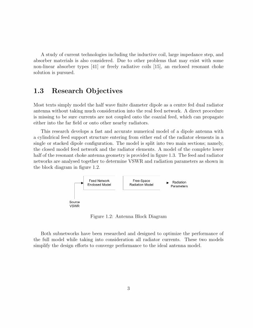
This research develops a fast and accurate numerical model of a dipole antenna witha cylindrical feed support structure entering from either end of the radiator elements in asingle or stacked dipole configuration. The model is split into two main sections; namely,the closed model feed network and the radiator elements. A model of the complete lowerhalf of the resonant choke antenna geometry is provided in figure 1.3. The feed and radiatornetworks are analysed together to determine VSWR and radiation parameters as shown inthe block diagram in figure 1.2.

Figure 1.2: Antenna Block Diagram

Both subnetworks have been researched and designed to optimize the performance ofthe full model while taking into consideration all radiator currents. These two modelssimplify the design efforts to converge performance to the ideal antenna model.

3

Figure 1.3: Antenna Mechanical Model4

1.4 Thesis Organization

The organization of this document is sectioned by chapter. The content of each chapter isspecified as follows.

Chapter 1 contains an introduction to the research objectives.

Chapter 2 provides an in-depth literature study. A theoretical analysis of the completecurrent choking solution is developed leading to a numerical implementation. This is thebasis for the numerical methods algorithm used in the discussion of future chapters. Areview of numerical errors is also given at the end of this chapter.

Chapter 3 validates the MoM code using simple structures with solutions obtainedusing analytical formulas and FEM codes. This includes the expected performance of thecore antenna elements including the dipole of finite radius and matching balun design. Italso covers overall antenna design including the feed line current choke. Validation of thegeneral MoM antenna model using FEM solvers is completed.

Chapter 4 compares the antenna prototype assembly measurement results with numer-ical solutions. Design for Manufacturing (DFM) procedures are detailed as well.

To conclude this research, chapter 5 covers lessons learned, a research summary, andfuture research possibilities.

5

Chapter 2

Theoretical Analysis and Simulation

2.1 Introduction

In order to have an efficiently radiating antenna, both the enclosed feed network andfree space radiation elements must be evaluated individually. In this chapter, the dipoleradiator elements are analysed, which includes the outer conductor of the coaxial feed line.

Reflection of voltage due to mismatch and unwanted currents coupled onto the feedor other conductive elements can severely degrade performance. Therefore, the matchingfeed balun, tuning element, and all exterior elements must be taken into consideration inthe full antenna design.

The following section reviews published literature on solutions that progress towards afully integrated resonant choke dipole. Other implementations to minimize feed currentsare also studied. This research will allow the designed antenna performance to approachthat of its ideal center fed theoretical counterpart.

2.1.1 Current Choking Solution

In a textbook analysis of a cylindrical dipole antenna, the feed network is generally ignored.It is assumed that the source is located at the center of the dipole. Not only does this causea problem with simulating the actual performance of the antenna, but also causes issueswhen measuring real performance. This is due to near field radiator currents propagatingdown the feed line and radiating out into the far field, which is significant for mostlyomnidirectional antennas [30].

6

To isolate the feed network from the radiator, a resonant choking structure is imple-mented. In general, the current choke must be designed while taking the antenna’s nearfield radiation into consideration. First, the resonant choke structure is studied.

Resonant Choke

The resonant choke is a purely metallic device that prevents leakage currents to travel downthe feed line and radiate destructively to degrade antenna far field performance. Whennot present, reduced performance is expected in the theta cut-plane of the dipole antenna[21]. It has been demonstrated that some current choking structures are highly resonantin nature when placed near the radiating element and are used effectively to isolate otherradiators or metallic surfaces. Antenna tunability is mostly dependant on the position anddimension of the resonant choke [38].

To prevent passive intermodulation, the antenna is constructed from entirely metallicsurfaces with no dielectrics. If solder joints and welds are done carefully, this allows near-byantennas to radiate at other frequencies without the concern of modulated carrier productsto land inside other receive bands [41]. Multiple stacked antennas can also be constructedto radiate multiple bands from the same antenna support structure or with separate feeds[3]. This also allows the antenna to support high power operation [50].

Both the absorber and metallic choke have been verified through measurement and canbe visualized in figure 2.1. This figure illustrates the magnetic field distribution of bothtypes of metallic choke and absorber methods using a patch antenna. It is observed thatthe folded structure of the current choke geometry reduces currents significantly and canhave a similar or greater effect than the ferrite absorber method at resonating frequencies.This implementation does not take into consideration the overall antenna radiation charac-teristics and since it has not be designed to be integrated into the patch radiator, radiationperformance can still be significantly reduced in comparison to predicted RF performance.

Figure 2.1: Current Choke and Absorber Magnetic Fields for Patch Antenna [21]

7

A resonant choke structure must be integrated with the radiator. In literature, currentsinside the choke are very low with respect to the currents along the main radiators. Toenhance the performance of the dipole, the internal choke structure is used to resonatewith the antenna. This method creates a large effective inductance at the choke boundary.Since currents resonate within the choke geometry, current located on the outer radiatorportion of the choke tend to zero. The full radiative numerical model is shown on the rightside in figure 1.3.

In contrast to the resonant choke, other types of chokes can be implemented by simplyadding an impedance step or coil inductance between the largest radiator and the feed orother radiators. This helps prevent near fields from coupling onto the line, but requires avery large radiator [50] or large inductive element. Since the choke geometry is smaller inlength than the dipole arm length, this is implemented as part of the design between theresonant choke and the feed line/support structure as shown in figure 1.3 as ’step 2’, butis not the core method to reduce currents at the edge of the dipole arm.

The resonant choke solution has been implemented to create a band reject filter typestructure by using a folded balun inside an enclosed coaxial type device, which supports thefeed coaxial line [18]. This, however, does not address currents accumulating on the outercylindrical conductor and propagating onto other metallic elements, which shifts radiationperformance. Other implementations demonstrate a folded choke that extends inside partof the radiator. This works well when the radiator radius is quite large; otherwise, nearfields are still trapped on the feed line or support structure [50].

To explore the possibility of using a resonant choke to reflect select frequency bandsback onto the radiators, the complete antenna is modelled as a circuit. It is possible toaccurately model the dipole pairs as a transmission line [44]. This theory is used to modelthe entire antenna as a quasi-static KVL circuit. Using the method of moments numericalsolution, the coaxial resonant choke can be easily inserted in the dipole antenna model.

Internally, the geometry of the choke structure can be modelled as a stepped coaxstructure as depicted in figure 2.2. It is numerically modelled using lumped element trans-mission line theory. This is shown as an enclosed microwave component consisting of twocoaxial lines, a coaxial step discontinuity, and a short at one end which makes it act likean enclosed coaxial resonator. Radiative currents are not required to be computed in thisstructure because it is enclosed. Thus, there is no worry of it radiating into free space.Only the effective input impedance at the interface is required to add to the MoM modelto compute currents along the exterior radiator, which is amplified by the resonant natureof this type of choke.

The inner choke radius is designed to be larger than the dipole arms to add to the

8

overall boundary inductance. This has an implementation limit since the outer conductorof the choke cannot be too large. The characteristic impedance is reasonably designedto match the radiator. The step discontinuity at the midpoint of the choke acts as alarge capacitance or a large inductance at the Zcb boundary, which pushes the supportradius to be small. Resonant effects of this choke also are observed to add additionalinductance at the boundary interface due to the structures’ approximate quarter wavereflection characteristics.

Figure 2.2: Choke Geometry Diagram

Although they are not as effective, inductive steps, coils, and absorber solutions canalso assist with choking currents along the feed line. Their advantages and disadvantagesas compared to the resonant choke structure is studied.

Absorber Solution

The ferrite absorber can act relatively efficiently as a current absorber. While there canbe improvements to ferrite absorbers by different manufacturing techniques, this type ofsolution is used as a comparison to the metallic resonant choke solution.

There are many advantages to using an absorber to reduce the magnetic field strengthon the feed line. Due to their wideband absorbing characteristics in VHF band, dipole

9

antennas can be tuned without too much effort. These absorbers may offer a compact andsomewhat lightweight option.

However, ferrite absorbers are non-linear in nature. Due to the fact that most antennainstallations have a passive intermodulation requirement coupled with the probability ofmany microwave sources in relative proximity to the installation site, a purely metallicsolution is preferred to allow better control of this phenomenon.

An absorber could be installed as in figure 2.3 to prevent currents from continuing ontothe feed. This has proven to be very effective to allow correction to radiation characteristicsand VSWR [43, 23].

Figure 2.3: Current Absorber at Dipole Ends

Although the current absorption is highly dependant on the material properties, anattempt is made to simulate these materials on the dipole structure in a typical case. Theresults of the simulation study are presented in chapter 3 for the purposes of a compari-tive study. In addition to the resonant choke and ferrite absorbers, impedance step andinductive coil solutions also have been considered.

Impedance Step and Inductive Coil Solution

Large impedance steps and inductive coils are frequently used to isolate the feed networkfrom the radiating element or stacked dipole antennas. Due to the quasi-static nature ofVHF/UHF dipole antennas, impedance steps or inductive coils can be used as a simplenon-resonating current choke to try and isolate currents from the radiator elements. Thistypically works best when frequency bands are close. Inductive coils have a significanteffect on the wideband match of the overall antenna; however, current distributions areseen to significantly shift antenna directivity due to the accumulation of currents on otherareas of the radiator [15].

10

Essentially, the additional current density on other elements are the root cause of theshifted far field radiation problem. This can be seen by the current distribution plot ofa resonating frequency for one resonating element. The current distributions in figure 2.4shows the radiating dipole along with strong leakage currents forming on the other radiatorelements. Ultimately, the leakage currents on other resonant elements could be formed onthe feedline.

Figure 2.4: Current Distribution of a Coil Loaded Dipole Array (left: Antenna Geometryright: Current Distribution) [16]

It is clearly visible from figure 2.5 that leakage currents onto other radiator resonatingelements affect the far field radiation patterns [16]. In terms of antenna radiation perfor-mance, these leakage currents can cause a significantly shifted and reduced performance incomparison to the antenna’s ideal model.

In comparison to the resonant choke solution, the resonant choke dipole antenna willlose bandwidth due to the resonant effect of the entire structure (ie: the antenna’s Q-factorwill increase). It has been found that inductive coils can increase bandwidth if the coilsare moved to the dipole radiator ends due to the additional current charge density there.When unshielded, this has a significant effect on radiation characteristics. However in theresonant choke model, the coaxial diameter increases to add to the charge accumulationeffect and increase inductance. This does not disturb the antenna radiation characteristics

11

Figure 2.5: Shifted Radiation Patterns Due to Leakage Currents [16]

since the additional currents are enclosed by the resonant coaxial structure structure asshown in figure 2.2 above.

2.1.2 Simulation Tools using Numerical Analysis

As in other typical antenna problems, several simulation tools may be used to simplify orsolve an antenna problem more efficiently. Greater depth to understanding sources of erroror fundamental knowledge of the problem by splitting the problem into parts allows fordesign innovation. In this research, the final numerical model is assembled systematicallyby combining the radiation model with the feed scattering parameter matrices produce theantenna’s overall characteristics, as illustrated in figure 2.6.

Each section of the antenna problem may be solved using several simulation tools. Intheory, FEM may be used to solve the complete problem. This, however, can be quitedemanding in terms of computational resources. To analyse and optimize the overallantenna problem, each section is solved using its best-known numerical technique. Thisallows for a quick design of independent problems and assemble the complete problem withlittle final optimization.

12

Due to the nature of the problems given by the code developed and results produced bycommercial electromagnetic (EM) solvers, Matlab is frequently used to easily and efficientlymanipulate numerical matrices to solve radiation problems and combine overall scatteringparameters [46]. Numerical electromagnetic simulators used to compute the theoreticalantenna performance in a vacuum space have their own advantages and disadvantages.These will now be discussed.

2.2 Radiator Numerical Solvers

Both Method of Moments (MoM) and Finite Element Method (FEM) solvers are usedto solve and optimize the antenna solution. Both numerical solvers offer advantages anddisadvantages in terms of speed versus accuracy [24]. In this research, the most efficientway to solve radiation problems, while taking the near field into account, is by usingsymmetry. In this case, the Method of Moments offers many advantages to quickly andefficiently solve the free space antenna problem. This inspired a custom MoM code to bewritten in Matlab to research the effect of different configurations. Other efficient codesusing axial symmetry about the center axis parallel to the radiator include commerciallyavailable FEM codes such as Comsol Multiphysics [14], but still use larger matrices to solvethe same problem.

13

Figure 2.6: Antenna Solution Block Diagram

14

2.2.1 Method of Moments Mathematical Model

We start the Method of Moments analysis by segmenting the radiator into its most simpleform. That is, a cylindrical scatterer with sections of changing radii [20]. Each of theantenna sections are labeled as Jn, as depicted in figure 2.7.

Figure 2.7: Segmented Dipole Antenna Model

The cylindrical radiating surface is assumed to be PEC so that [7]

~Et = ~Ei + ~Es = 0 (2.1)

where ~Ei and ~Es are the incident and scattering electric field vectors respectively. Thescattering electric field is used to compute impedance along the cylindrical scatterer. Itcan be derived from the vector potential ~A for which

15

~A2 + k2 ~A = −µ~J (2.2)

using the standard Lorentz condition on Maxwell’s equations. The above equation can besolved for ~A to obtain the relation

~A =µ

4π

∫∫∫V

~Je−jkR

RdV ′. (2.3)

where G(z, z′) = e−jkR

Ris known as the free space Green’s function [20]. Using the scaler

and vector potentials, Maxwell’s equation for ∇× ~E can be reduced to its differential form

~Es = −jω( ~A+1

k2∇(∇ · ~A). (2.4)

While neglecting edge effects and only considering the radiating surface, the above equationcan be reduced to it’s scalar form

Esz = −j 1

ωµε(k2Az +

∂Az∂z

) (2.5)

with Az computed as

Az =µ

4π

∫∫S

Jze−jkR

RdS ′ (2.6)

where R = (ρ2 + a2 − 2ρa cos(φ − φ′) + (z − z′)2)1/2 and φ = 0 for this axisymmetricalproblem. Also note that primed and non-primed values indicate source and field pointsrespectively. It is now possible to combine equations 2.5 and 2.6 to produce the scatteringfield integral equation

Esz = −j 1

ωµε(k2

µ

4π

∫∫S

Jze−jkR

RdS ′ +

∂

∂z

µ

4π

∫∫S

Jze−jkR

RdS ′). (2.7)

16

The free space magnetic field can be computed from Maxwell’s equations [24]

~H = − 1

jωµ∇× ~E (2.8)

and the line current down the PEC radiator can be computed from the following vectorequation

~Js = n× ~H, (2.9)

or in the scalar form

|Jz| = |(n× ~H) · z| = |(x× ~H) · z|. (2.10)

In the second term of equation 2.7, the partial derivative and the integral can beinterchanged to combine both integrals. Also, if a is kept small enough, the assumptionthat ρ = a can be applied. It is a rule of thumb that a << λ [7]. This will be a sourceof error in the Method of Moments code, which is discussed later in the chapter. Es

z thenbecomes

Esz = −j 1

ωµε

∫Jze−jkR

4πR5[(1 + jkR)(2R2 − 3a2) + (kaR)2] dz′. (2.11)

It can be noted here that the above equation will need to be solved by segmentationdue to the Jz term. This allows for the Jz term to be extracted from the integral as aconstant term for each segment of the antenna. The antenna radiator segmentation isshown in figure 2.7 above. It is also noted that surface current term can be substitutedwith the location of the impedance term at the center of the radiator by reciprocity. Thisallows for the ρ in the equation for R to be zero, which leaves R = (a2 + (z − z′)2)1/2.

Solving equation 2.1 for ~Ei, equation 2.11 can be solved for the incident field that isnow located at ρ = a

In(z′n)

∫δn

e−jkR

4πR5[(1 + jkR)(2R2 − 3a2) + (kaR)2] dz′ = −jωεEi

z(ρ = a). (2.12)

17

where n is the segment number along the radiator. The above equation is a convenientform to compute filament line currents along the radiator [7].

A virtual coaxial source is used as a field potential Eiz with ρ = a as the center conductor

radius and the outer conductor defined by the impedance required at the source. Thisvirtual source is depicted in figure 2.8. The gap given by [51]

Figure 2.8: Source Definition

Ei ' −Vs(k(b2 − a2)e−jkR

8loge(ba)R2

(2(1

kR+ j(1− b2 − a2

2R2))

+a2

R((

1

kR+ j(1− b2 + a2

2R2))(−jk − 2

R) +−1

kR2+ j

b2 + a2

R3)))

(2.13)

The above equation can be simplified for electrically small radii, which removes the ρdependence. Therefore, the new applied electric field is given as [51]

Ei =−V s

2 log( ba)(e−jr1

r1− e−jr2

r2) (2.14)

where r1 = (z2 + a2)(1/2) and r2 = (z2 + b2)(1/2). The applied electric field Ei or moresimply, the segment source voltage [Vm], is defined as a field applied along the length of

18

the radiator. The source input is defined as magnetic frill located at the centre of thedipole. It can be defined either with or without ρ dependence given the symmetry of theproblem [51]. Should the geometry be more complex, higher order modes above TEM maybe added to reduce the error of the applied electric field [20, 11].

The equation 2.12 can be reduced to the form

N∑n=1

In(z′n)Zn = −Ei, (2.15)

where N is the total number of segments along the radiator, I is the segment current, Znis the segment impedance, and Ei is the source.

In this case, a KVL method is most conveniently used by computing impedances alongthe radiator surface [44]. This allows for internal structures to be added to the radiatorimpedances. The equation 2.15 as shown in figure 1.3 can then be implemented in matrixform as

[In][Zmn] = [Vm], (2.16)

where [Vm] is defined as the applied electric field along each segment of the radiator, [Zmn]is the impedance, and [In] is the unknown current distribution. In this form, internalcoaxial choke Zin impedance can be inserted into its respective Zm,n’th element. Solvingthe above equation, the final solution is quite simply

[In] = [Zmn]−1[Vm], (2.17)

and [Zmn] can be expanded as a 2D matrix from a 1D segmentation [Zk] along the radiatoras follows

Zm,n =

Z1 Z2 · · · ZkZ2 Z1 · · · Zk−1...

.... . .

...Zk Zk−1 · · · Z1

(2.18)

19

for Z1 starting at −l/2 and Zn ending at l/2 and [Zk] defined as

[Zk] =

∫δn

e−jkR

4πR5[(1 + jkR)(2R2 − 3a2) + (kaR)2] dz′. (2.19)

2.2.2 Matlab Implementation

The current can be numerically computed at each segment of the radiator using 2.17.Matlab is used to implement matrix equations 2.17, 2.18, and 2.19 with the source definedin equation 2.14. The commented source code is given in appendix I. Some useful open-source tools for electromagnetics were found on the matlab webpage [34] and also in otheropen-source packages [39].

Packages used to convert [ABCD], impedance, and scattering parameter matrices al-lowed quick system design for the overall antenna. See Appendix I for additional detailsconcerning antenna system computation.

Coaxial Line

Typically, the dipole antenna is connected to the transceiver with a coaxial cable. Fromchapter 2, the ABCD parameters of a lossy coaxial can be easily computed numericallyand inserted into the overall antenna system. These computed scattering parameters arecombined directly with the antenna Balun.

Additionally, the coaxial cable not only acts as the feed line that carries energy tothe radiator, but its outer conductor also re-radiates RF energy from currents coupled bythe antenna’s near field. As a design goal, a cylindrical support structure is designed toenclose the feed cable inside. The support pipe isolates the feed coaxial cables from coupledcurrent. This also provide a rigid structure to attach the dipole to the support structureas shown in figure 1.3.

For the straight coaxial sections, the ABCD parameters can be computed using thedimensions of the waveguide. The ABCD parameters are given by [42]

[ABCD] =

(cos βl jZ0 sin βl

j 1Z0

sin βl cos βl

)(2.20)

20

with β and Z0 defined as the the waveguide propagation constant and the waveguideimpedance respectively. β and Z0 can be computed from the transmission line character-istics of a coaxial line. This is given by [42]

Z0 =√

(R + jωL

G+ jωC) (2.21)

β =√

((R + jωL)(G+ jωC)) (2.22)

where for a coaxial waveguide

L =µ

πloge(

b

a), (2.23)

C = 2πε′

loge(b/a), (2.24)

R =1

2πσ tan δ(1

a+

1

b), (2.25)

G = 2π2fε′′ loge(b

a). (2.26)

Resonant Choke Circuit Model

To insert the choke model into the MoM code, a circuit model is used. The coaxial chokestructure is analyzed by combining the scattering and impedance parameters of each ofthe individual components [46]. A general circuit model of this device is shown in figure2.10. Since the waveguide between discontinuities is somewhat electrically large, a simplecircuit approximation of the coaxial step discontinuity is used [47]. More accurate modelscan be modelled by the Mode Matching method should the geometry extend out of theusable range of the circuit approximation [40]. The capacitance of the coaxial circuit modeldiscontinuity is given by

21

Figure 2.9: Choke Circuit Diagram

Cb =ε

π[α2 + 1

αloge

1 + α

1− α− 2loge

4α

1− α2]. (2.27)

The resonant characteristics of this shorted structure of the coax 2 section adds sig-nificantly to the effective inductance at the interface boundary. The resonant section isinserted using a parallel resonator configuration as shown in figure 2.10 where Zres is givenby

Zres = (1

jωLr+ jωCr)

−1. (2.28)

Finally, the addition of all impedances and transmission lines are used to compute theZin of the resonant choke model. This frequency dependant value is inserted into the chokeresonator discontinuity point of the MoM numerical code.

Figure 2.10: Resonant Circuit Model

22

As an additional note, the interface to the choke component can be thought of as aninfinitely long centre conductor protruding out of the coaxial line. Higher order fringingfields at the interface of this model can be expected, but are assumed small in this model[8]. This could be another source of error.

2.3 Feed Network Analysis

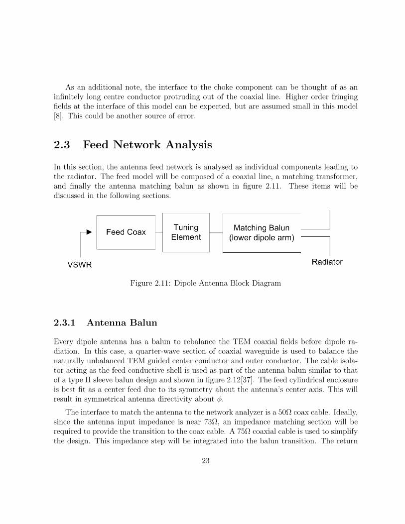
In this section, the antenna feed network is analysed as individual components leading tothe radiator. The feed model will be composed of a coaxial line, a matching transformer,and finally the antenna matching balun as shown in figure 2.11. These items will bediscussed in the following sections.

Figure 2.11: Dipole Antenna Block Diagram

2.3.1 Antenna Balun

Every dipole antenna has a balun to rebalance the TEM coaxial fields before dipole ra-diation. In this case, a quarter-wave section of coaxial waveguide is used to balance thenaturally unbalanced TEM guided center conductor and outer conductor. The cable isola-tor acting as the feed conductive shell is used as part of the antenna balun similar to thatof a type II sleeve balun design and shown in figure 2.12[37]. The feed cylindrical enclosureis best fit as a center feed due to its symmetry about the antenna’s center axis. This willresult in symmetrical antenna directivity about φ.

The interface to match the antenna to the network analyzer is a 50Ω coax cable. Ideally,since the antenna input impedance is near 73Ω, an impedance matching section will berequired to provide the transition to the coax cable. A 75Ω coaxial cable is used to simplifythe design. This impedance step will be integrated into the balun transition. The return

23

Figure 2.12: Design Based on Type II Sleeve Balun [37]

loss goal of the this section is also made low enough to be sure the performance of thebalun does not affect the overall antenna performance.

To step from the coax feed cable to the outside radiators, an internal coax structurewas designed as shown in figure 3.20. The design was kept simple as an air filled coax thatneeded to be near the ideal impedance of a dipole. The results are presented in Chapter 3.

2.3.2 Tuning Element

A tuning element can be used to match the radiator input impedance over a wider frequencyrange. In this case, a simple stub tuner is designed and inserted just before the balun [42].The advantage to using a stub tuner is its compact shape. It is implemented by solderinga shorted coaxial cable to the main coaxial feed line at a distance from the source point.

Figure 2.13: Tuning Circuit [42]

24

Once the initial measurements of radiator and balun are complete, the s1p file generatedis used with the coaxial cable characteristics in a circuit simulator to match the antennaover a wider frequency band.

2.4 Sources of Error

Several different solvers are used to examine the dipole choke problem and validate themethod of moments code. Each numerical implementation has its own advantages anddisadvantages with respect to computational efficiency. Since it is never possible to havelimitless hardware resources, a discussion of the significant sources of error allows betterunderstanding of the design direction.

Validation of the different simulation methods is required to be certain that measuredresults will be close to those simulated. Due to the nature of this problem, it is difficultto remove all sources of error in simulation and measurement. The latter is discussed inChapter 4.

2.4.1 Sources of Error in MoM Codes

As discussed above, it is possible to encounter numerical error with simplified MoM codes.A significant source of error is generated at the radii step discontinuity and resonator L/Cvalues. While developing a robust MoM code that solves the dipole model including thechoke, the enclosed coaxial-type structure will have higher order modes generated at theinterface. This causes fringing fields in this area that will have a global effect on theantenna problem.

Other sources of error include those found by simplifying the source to be electricallysmall. This can add significant error to radiators with large radii. In this case, the outerchoke surface could contain some sources of error; however, this area is less significant sinceit is located electrically far from the source and has a low current distribution due to theeffect of Zcb.

2.4.2 Sources of Error in FEM Codes

Numerical computational error can be significant for FEM if there is insufficient meshin the problem. In FEM codes, adaptive meshing allows s-parameters to converge where

25

fields are changing radically. In particular, HFSS requires manual seeding of radiationboundaries to achieve acceptable results with respect to directivity and gain plots sincethey are not required for convergence using the default solver values.

In order to guarantee that radiation parameters are converging and computationalerror is reduced, computation volumes around the antenna should be grown to verifyconvergence. It is found through numerical experimentation that the radiation boundaryshould be located approximately λ/2 away from the largest radiator in the direction of themain lobe for reasonable results.

2.4.3 Sources of Error in Lumped Element Codes

Lumped element codes generally function over a very limited range of geometry. Extend-ing past the recommended working range results in larger error. S-parameters obtainedfrom these codes can be verified using Mode Matching techniques; however, they requiresignificant efforts to implement numerically. Commercial software such as Microwave Wiz-ard or Fest3D may be used in lieu of Lumped Element to add flexibility to the numericalcode without sacrificing accuracy or computational speed over FEM codes. These codescould also model the resonator section quite accurately, which improves the overall antennasimulation model.

26

Chapter 3

Radiator and Feed NetworkSimulation

The method of moments algorithm is known in the antenna design community as beingone of the most efficient methods to solve free-space radiation problems. As shown in theprevious chapter, the method can also be used to include internal structure impedanceswhile taking outer geometry radiation characteristics into consideration. This allows theresonant choke internal geometry to be modelled and inserted into the MoM code.

The radiator and feed network simulation models can be implemented using the the-oretical analysis defined in the previous chapter. The MoM model is first validated bycomparing to a similar FEM model using Ansys’ HFSS [5].

3.1 Method of Moments Simulation Model

In both the MoM and FEM center-fed dipole models, the feed network is neglected, whichallows some validation before constructing the full antenna simulation model.

3.1.1 VSWR and Directivity of a Finite Radius Dipole Antenna

To validate the MoM code written in Matlab [34], an ideal dipole is computed using thenumerical integral equation for a finite diameter cylinder as described in chapter 2. Fromequation 2.17, the input impedance can be computed by

27

Zin = Vin/Imid, (3.1)

for which Imid is defined as the segment current computed at the center or midpoint of theradiator.

Once Zin is computed, the input impedance is converted to a reflection coefficient, Γ,and finally to VSWR. Note that VSWR reference impedance is 75Ω in all validation plots,however, a balun is designed for a 50Ω coaxial impedance for the choke dipole antenna.Finally, the ideal current distribution along the radiator is computed for several differentlengths. The directivity is then computed and compared to the HFSS model.

3.1.2 Radiator Effective Electrical Length

It is expected that the added radiator geometry to prevent currents onto the feed line willhave a significant effect on the electrical length of the dipole arms. An overall smallerbandwidth for dipole arms of similar length compared to its ideal counterpart is expected.To illustrate this effect, the magnitude of the current distribution along the antenna mustbe visualized. All finite radius dipole lengths are shown in terms of λ where the a centerfrequency of 125MHz is found for R = 0.9375in, λ = 42in, and Gap = 1in.

Ideally, | ~Jz| tends to zero along the top and bottom of the dipole. This is confirmed infigure 3.1 and 3.3 as the current clearly tends to zero at the ends of the dipole arms forλ/4, λ/2, and λ lengths. This will be the design goal to satisfy the research objectives.

The directivity at center frequency is also compared. It is observed that the errorbetween the plots increases as the arm length increases. This appears to be due to theincreased number of tetrahedra in the finite element model with respect to the increasein computational air volume. It has been observed that directivity plots can decrease inaccuracy unless a very large air volume is used. This is another advantage to use methodof moments since the directivity is derived from the line currents along the radiator whilecomputationally, the surrounding volume is assumed free space.

28

Figure 3.1: MoM Ideal Dipole Current Distribution (left: λ/4 center: λ/2 right: λ)

Figure 3.2: HFSS Ideal Dipole Current Distribution (left: λ/4 center: λ/2 right: λ)

29

Figure 3.3: MoM vs HFSS Ideal Center-fed Dipole Directivity (left: λ/4 center: λ/2 right:λ)

3.1.3 Radius of the Radiator Arms

In theory, the dipole is analyzed for a zero radiator radius, which allows the computationof the exact field equations generated by the antenna [7]. In practice, the radius of theradiator arms is non-zero and must be optimized for a frequency band. The code inAppendix A can be used to compute the antenna parameters of a simple dipole for severaldifferent radii. Both VSWR and directivity vs frequency is computed for several radii asshown in figure 3.4. An optimal design is found to be around 1”

3.1.4 Gap Spacing Between Radiators

The gap spacing is also analysed as a design parameter. The resonant frequency can besignificantly shifted by manipulating the gap space between the dipole arms. It’s visiblefrom the plots in figure 3.5 that by increasing or decreasing this parameter, the resonanceshifts higher or lower in frequency respectively. This can naturally degrade VSWR for gapsizes that are too large.

30

Figure 3.4: VSWR and Normalized Directivity for Several Radiator Radii

Figure 3.5: VSWR and Normalized Directivity for Several Radiator Gaps

31

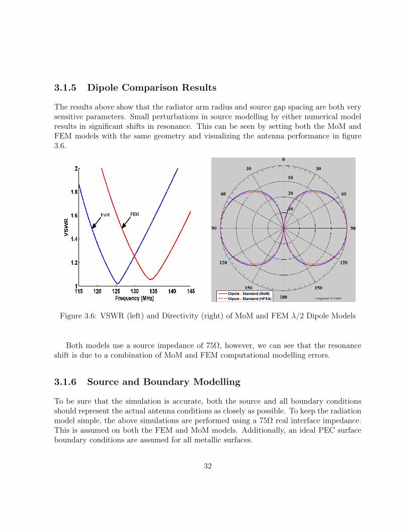
3.1.5 Dipole Comparison Results

The results above show that the radiator arm radius and source gap spacing are both verysensitive parameters. Small perturbations in source modelling by either numerical modelresults in significant shifts in resonance. This can be seen by setting both the MoM andFEM models with the same geometry and visualizing the antenna performance in figure3.6.

Figure 3.6: VSWR (left) and Directivity (right) of MoM and FEM λ/2 Dipole Models

Both models use a source impedance of 75Ω, however, we can see that the resonanceshift is due to a combination of MoM and FEM computational modelling errors.

3.1.6 Source and Boundary Modelling

To be sure that the simulation is accurate, both the source and all boundary conditionsshould represent the actual antenna conditions as closely as possible. To keep the radiationmodel simple, the above simulations are performed using a 75Ω real interface impedance.This is assumed on both the FEM and MoM models. Additionally, an ideal PEC surfaceboundary conditions are assumed for all metallic surfaces.

32

Specifically for the FEM model, radiation boundary conditions are given to the limitsof the bounding air cylinder containing the antenna geometry. Additional minimum refine-ment is specified on the radiation boundary to improve accuracy. Although this improvesthe model, a degradation in directivity performance is shown for this electrically largeproblem.

3.2 Feed Line Effects

The main purpose of this research is to analyse and prevent the accumulation of feedline surface currents. These surface currents are generated once a metallic line passesnear/through either end of any dipole antenna. This is illustrated in figures 3.7 and 3.8 bynoting the red color, which indicates large surface currents.

Figure 3.7: Dipole Feed Line Currents without a Choke or Absorber

33

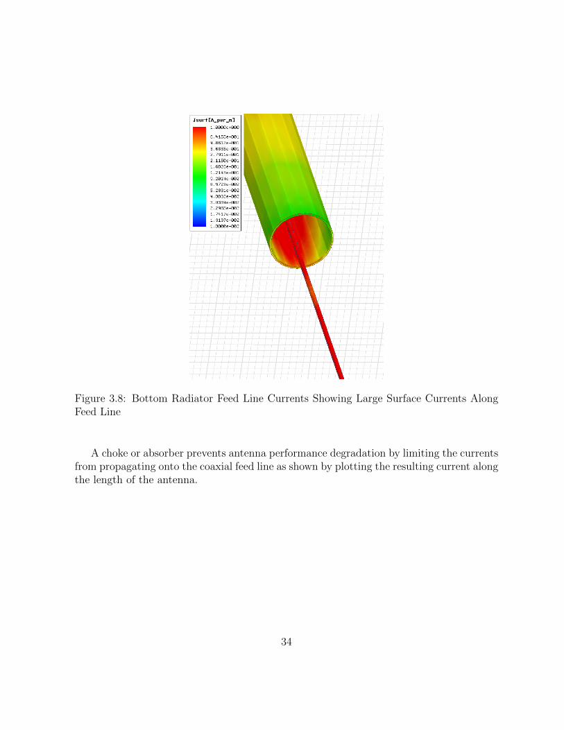
Figure 3.8: Bottom Radiator Feed Line Currents Showing Large Surface Currents AlongFeed Line

A choke or absorber prevents antenna performance degradation by limiting the currentsfrom propagating onto the coaxial feed line as shown by plotting the resulting current alongthe length of the antenna.

34

3.3 Dipole Antenna Design

Both absorber and resonant choke designs are used in literature. In the dipole antennadesign process, the absorber and resonant choke are both analyzed individually and com-pared. Since the absorber is known to absorb EM energy over a wider frequency band, itdoes not require much tuning. It can be simply added onto the feed line network and thedipole can be tuned by adjusting the gap spacing for a selected radiator radius and length.

3.3.1 Absorber

A FEM model of the absorber dipole antenna is created to compare the approximateperformance with the resonant choke dipole antenna. It should be noted that HFSS canonly model nonlinear materials accurately if all the electromagnetic material propertiesare known. Since there are large variabilities to the doping of ferrite materials, simulationaccuracy is limited.

The performance seen in the lab is expected to be significantly different than what iscomputed by HFSS. Nevertheless, HFSS is still used to compute approximate performancefor comparison purposes. An open ended dipole antenna is simulated with a cylindricalferrite material added to a section of the feed line.

The volumetric currents in the material are clearly dissipated as shown in figure 3.9. Itis expected that as currents travel farther from the dipole that they tend to zero. Naturallyif the cylindrical material is made larger, the absorbing effects are higher, which may alsoallow for shorter absorbers.

35

Figure 3.9: Volumetric Current, | ~J |, in the Absorber

36

Using HFSS’ calculator feature [4], | ~Jz| is computed along the radiator with the resultspresented in figure 3.9. Plots of the currents along the length of the antenna with andwithout the absorber material indicates a significant reduction with the additional materialas shown in figure 3.10.

Figure 3.10: Radiator Current Distribution (left: No Absorber right: Absorber Installed)

Currents that propagate down the feed line can radiate into free space, which sig-nificantly affects the far field patterns of the antenna. As a direct result of the currentdistribution along the feed line, the directivity is severely altered as shown on the left sideof figure 3.11. Once the absorber is installed, the dipole currents are significantly reducedat the dipole end and the far field performance is regained as shown on the right side offigure 3.11.

The absorber is a simplified means of correcting unwanted currents around the radiatorends for wideband applications. It is seen, however, that the currents along of the feedline are larger and cannot necessarily be tuned at any given frequency. The advantageto a choke model is that the antenna is tuned for the operating frequency band whilesimultaneously providing a current-free distribution along the feed cable.

37

Figure 3.11: Radiator Current Distribution (left: No Absorber right: Absorber Installed)

3.3.2 Choke

The choke solution uses a resonant structure as described in chapter 2 and shown infigure 1.3 to reduce currents along the feed line and reshape the fields to maintain anomnidirectional far field pattern. Internally, currents along the dipole arms continue intothe resonant choke, which allows the creation of an effective inductance at the boundaryas discussed in chapter 2. This works especially well when the coaxial choke is tuned alongwith the dipole arms as one unit. To be sure this happens, the characteristic impedance ofthe choke boundary is designed to match the radiation impedance of the antenna. To matchthe VHF antenna tuned to 125MHz, the optimal design was found to be at 68.2Ω. Thecapacitive step is kept as large as possible using the support pipe as the inner conductor.

Using the choke, antenna support, and dipole arm geometry, both the MoM and FEMsimulation models are constructed in the matlab code and HFSS respectively. Similarly tothe MoM model, line currents computed in the HFSS model are computed along the edgeof the antenna radiator as given in figure 3.12.

Since this device does not rely on non-linear materials to absorb currents near thedipole ends, the results should be similar to those found in a center fed case. The currentsare computed along the radiator for both the standard finite radius center fed model and

38

Figure 3.12: Current Computation Along the Radiator

the coaxial feed line finite radius model. The results are computed and compared in figure3.13. The currents over extend onto the outer choke geometry, which add to the overalleffective length of the dipole antenna.

To correct the increased electrical size of the resonant choke antenna, the arm radiusand gap distance is kept the same while the ideal center fed arm length is corrected by 0.5into recenter the resonance to that of the choke model. This allows for an easy comparison ofbandwidth changes relative to the same center frequency. It is also noted that the standarddipole current does not go to zero at the ends. This is also seen in the FEM models given infigure 3.3 above. Even though the effective radiator length is extended slightly, the chokeacts as a method to smoothly transition edge currents to zero, improving performance forthe finite radius model.

The results for VSWR and directivity comparing both the standard textbook dipoleand the resonant choke solution is given in figure 3.14. While the standard dipole has thesame gap distance and radius at the resonant choke model, the standard dipole arm lengthcorrected so that it is centered at the same center frequency.

The directivity at center frequency is also computed and compared to the standard cen-ter fed model. A close correlation between the two models is found. This is expected sincethe currents along the radiator are significantly attenuated due to the input impedance ofthe choke structure. Results are shown in figure 3.15.

39

Figure 3.13: Current Distribution Along the Radiator Comparison

40

Figure 3.14: VSWR and Directivity Over Frequency Comparison

Figure 3.15: Directivity at Center Frequency Comparison

41

Next, the VSWR and directivity results in the FEM simulation is shown in figures 3.16and 3.17 respectively. They can be also be compared to the ideal values found in figure3.6.

3.3.3 Choke vs Absorber

The FEM model of the choke and absorber is now compared. Using HFSS’ calculatorfeature, the radiator line current is computed along the support pipe containing the feedcoaxial cable. Comparing the low field sections of each prototype simulation model, thefigures 3.18 and 3.19 is produced for the resonant choke and absorber antennas respectively.

It is observed that choke model currents are significantly lower near the bottom ofthe support pipe at center frequency. Since the choke and dipole are both band limited,they work well when tuned together to a small operating band. Tuning the choke antennais simple since the effective electrical length of the dipole increases when the choke outercoaxial conductor is positioned further away from the antenna midpoint. This is consideredas a tunable feature along with the gap spacing at the source, which is easily implementedin a prototype model.

42

Figure 3.16: Choke Model VSWR Comparison

Figure 3.17: Choke Model Directivity Comparison

43

Figure 3.18: Choke: Current Along The Support Pipe

Figure 3.19: Absorber: Current Along The Support Pipe

44

There are many advantages and disadvantages to both the choke and absorber dipoleantennas. While the choke provides excellent dipole performance over a limited bandwidth,the structure itself is larger than the arm radius. Therefore, a radome covering the antennacould be heavy and costly.

Absorber models can offer slightly easier tunability since they only require adjustmentof the center gap for a fixed arm length and gap; however, their range is limited. The chokeallows for a larger range of tunability using the position of the choke along with the gapto add flexibility to the location of the antenna’s center frequency. This is at the expenseof using non-linear electromagnetic absorbing materials.

3.4 Feed Network Design

The feed network is designed to allow the dipole to operate efficiently in the requiredfrequency band. As discussed in chapter 2 and shown in figure 2.11, the feed networkconsists of a 50Ω coaxial cable, a matching balun, and a tuning element. The tuningelement is designed using the measured results of the antenna and is discussed in chapter4.

3.4.1 Balun Design

To design the antenna balun, all other radiative elements were removed and only the baluncoax structure was kept. A probe was designed to protrude perpendicular from the coaxcenter conductor to align probe currents with the coax electric field vectors [13]. As thedipole is simulated using a 75Ω input impedance, the output of the balun is designed tomatch the impedance. The bottom of the balun is shorted to remove the possibility ofadding leakage currents back onto the feed line. The enclosed balun structure is given infigure 3.20.

This allows for an excellent transition from the 50Ω feed line to radiator with wellmatched results shown in figure 3.21. With the available materials, the actual dimensionsof the coax become: RSupportP ipe = 0.5in OD, RRadiator = 0.8875in ID. A theoreticalimpedance of 71Ω with a quarter wavelength of 23.2in in the balun section is produced,which is close to the free-space quarter wavelength at 125MHz of 23.6in.

45

Figure 3.20: Balun: Enclosed HFSS Simulation with Radiator Component Removed

46

Figure 3.21: Balun: Return Loss

47

Chapter 4

Antenna Assembly and Measurement

A prototype of the choke and absorber versions of the dipole antenna were manufacturedand assembled. A general design is used so that it can accommodate both the resonantchoke and absorber dipole antenna types. Both units use the same base antenna specificallydesigned for ease of manufacturing and assembly. The versatility of the prototype can beseen the figure 4.1.

Figure 4.1: DFM Applied to Both Prototypes

48

The current choking structure was also simplified for ease of tuning on the bench. Theinternal radius cavity is hollowed due to its evanescent properties and low field strengthinside. This allows for easy movement on the bench for testing and tuning. A detaileddrawing of the choke is given in figure 4.3.

Figure 4.2: Manufactured Transition

Since the source is very sensitive to tuning, the prototype assembly was carefully de-signed to model the simulation as closely as possible. Figure 4.2 shows how it is takenfrom its block diagram model, to its manufactured prototype.

Only the choke model was tested for VSWR and relative gain measurements with bothdipole antennas mounted parallel to one another. The results are provided in the nextsection.

4.1 Prototype Antenna

The choke prototype was manufactured, assembled, and tested indoors at the WADEAntenna facility. The WADE Antenna Dipole model D5072 is used as a reference antennato test the prototype. Since the antenna is an uncalibrated reference antenna, additionaltests are recommended. Despite this fact, it is used to measure directivity with respect tofrequency and VSWR. A performance gain was achieved for small design bandwidths asshown in figure 4.4.

49

Figure 4.3: Resonant Choke Manufactured Prototype Structure

The as-built fully integrated HFSS model was constructed to compare tuned measuredresults. The HFSS model is given in figure 4.5, which includes the choke structure, thesupport structure containing feed cables, and the matching balun. It is observed that anarm length of 25in and a gap size of 2in for a center frequency of 125MHz reported byHFSS was too large. The method of moments code reports an arm length of approximately20in with a gap size of .5in. To correct for the detuned performance, figure 3.4 is used toincrease the center frequency by increasing the source gap distance. By correcting usinglarger gap sizes and repositioning the choke structure, the following results were achievedwith comparison between measured and simulated results in figure 4.6.

4.1.1 Additional Matching Section

As mentioned in Chapter 3, the matching section of this antenna is designed after initialantenna measurements are made. For an accurate antenna matching transformer, singleport touchstone file (S1P) is generated as close to the center of the AUT as possible andinserted to into the circuit as shown in figure 4.7 [42].

The circuit is then run through the optimizer to find the optimal lengths of D and Lshown in the figure. The distance from the end of the cable to the center feed of the AUTwas measured and added to the final length of D. Also, the exact cable characteristics

50

Figure 4.4: First Choke Prototype Measurements

Figure 4.5: HFSS As-built Model Including the Feed Network

were used in the simulator to represent the SM141 feed line coaxial cable as accurately aspossible.

The final computed lengths were found to be D=21.2in, and L=21.7in and the resultsfrom the simulator are shown in figure 4.8. These results of the simulated antenna assemblycorrelate with those found by measurement with the new tuning element.

51

Figure 4.6: VSWR Comparison of the HFSS Simulation vs Measurement

Figure 4.7: ADS Antenna Stub Matching Circuit

52

Figure 4.8: ADS Antenna Stub Matching Results

53

4.2 Test Repeatability and Sources of Error

Although numerical error can be significant for resonant devices, one of the significantsources of measurement error for VHF band dipole antennas are the manufacturing toler-ances, assembly errors, and the test setup.

4.2.1 Test Repeatability and Measurement Error

It is clear with the above results that one of the most important factors when measuringany microwave device or radiator is test repeatability. With an uncontrolled test site suchas a warehouse, it is difficult to maintain repeatable results. Resonant structures are alsoprone to detuning from manufacturing and assembly errors. This is especially true foromnidirectional antennas.

Due to the dipole’s natural omnidirectional gain pattern, all space around the antennathat is not coated with absorbing materials must be taken into consideration during tests(i.e.: ground, bench, walls, people, etc.). Constructive or destructive reflections returningon to the antenna will appear to increase or decrease performance respectively. Thisis generally frequency dependent and will look like small or large ripples in the resultsdepending on the scatterer. In either case, this reduces test repeatability and will produceerroneous results.

For an electrically large antenna such as the VHF dipole, a physically large outdoortest setup is recommended to remove most significant scatters. It, however, can be timeconsuming for tuning this type of antenna. Indoor sites offer the most convenient solution,but also can be error prone with unpredictable scatterers. Testing in a well controlledenvironment, such as using ferrite beds or electromagnetic absorbing cones surroundingthe antenna to prevent radiation reflection, produces the most repeatable results.

54

Chapter 5

Conclusion Summary, LessonsLearned, and Future Research

The purpose of this project was to determine the source of the dipole’s feed line currentsand to reduce those currents with prototypeable design. Through the use of many designtools, the current distributions, performance characteristics, and antenna properties weredetermined. The method of moments provided accurate results while reducing simulationtime to a fraction of that used by its finite element method equivalent model. Overall, theprocess allows for an understanding of the dipole antenna model using both a resonantchoking structure and absorbing materials along the coaxial feed line.

Once the antenna model was well understood, a manufacturable prototype was con-sidered to implement both design methodologies. Using Design for Manufacturing, a baseprototype was designed to implement the current choke dipole model, but also could sup-port additional research and test on an absorber model.

Finally, the resonant choke model was tested in the lab with results close to that ofsimulation for VSWR; however, mixed results were obtained for gain. Gain results provedthat the many scatterers in the lab changed the performance in unexpected ways in higherfrequencies.

55

5.1 Lessons Learned

Several lessons were learned during the course of this project. These are summarized below.

• The antenna design problem was easily managed by dividing the radiator, choke,balun, and tuning section into separate design stages. This sped up overall antennadesign and allowed focus on electrically sensitive areas.

• To accurately model antenna performance, source modelling must be thorough andmay require higher order modes such as the coaxial TE11 to add accuracy to thecurrent magnetic frill model.

• HFSS simulation model produced resonant frequencies higher than expected by mea-surement while the MoM produced results that were lower than expected. This ispartially due to the resonant nature of the choke structure, which produces variedeffective inductance at the enclosed interface boundary.

• Current coupling effects appear to be frequency sensitive and require multiple featuresto fully support wideband operation due to the choke’s resonant nature. Additionalresearch to allow multiple layers inside the choke could help widen bandwidth, butcould have a negative effect on high power handling due to the required small gapsizes for coupling between resonators.

• More research is required in absorber materials to use them in an optimized design.Further research was not conducted during this thesis due to the lack of electromag-netic properties for available materials and due to time constraints.

56

5.2 Future Research Possibilities

Future research possibilities on this project are possible in several areas of research. Theseare itemized below.

• Mode matching can be used to accurately model internal resonant choke structureas well as the the feed network. This could extend the design parameters to allowbetter flexibility and design accuracy.

• More tests required for full gain profile and more accurate test results using anoutdoor test side or chamber. Together with additional tests and simulation, im-provements can be made to the existing prototype to reduce size and complexity.

• A better simulation model for non-linear materials is also required to prevent un-expected test results. This could help reduce the effects of PIM and be a strongcompetitor to the resonant choke model in terms of overall antenna size. The MoMcode could be used as a starting point to implement such a model.

• Additional efforts to construct a more compact resonant choke design could help fitthe antenna into more traditional radomes. This could also assist with the structuralsupport of the stacked model.

• Design focus using multilayer chokes with better tuning methods could increase wide-band performance. Literature and simulation suggests that increasing the choke com-plexity could increase the number of resonances and lead to a stackable widebanddesign.

57

5.3 Conclusion Summary

The research goal to understand, design, manufacture, assemble, test, and tune a newtype of dipole antenna that eliminates currents when configured with a feed coax cableentering either end has been successfully achieved. Simulation and measurements producescorrelating results that led to a working design. The resonant choke not only proves toreduce currents lower than other models, but also removes the requirement for non-linearmaterials to be attached to the antenna. The new type of dipole model including the feednetwork shows that it can produce results quite close to those generated by the dipole’stheoretical center fed counterpart. For these reasons, the resonant choke dipole antenna isa top contender for single or stacked operation.

58

Appendices

59

Appendix A

Computer Codes

A.1 Method of Moments in Matlab

Matlab or Octave numerical software can be used with the following code to compute theresonant choke dipole antenna parameters such as VSWR, directivity, gain over frequency,and radiator currents.

A.1.1 Dipole System

Main entry point of the MoM code is given in this first section.

% File: dipoleSystem.m

% Purpose: Computes overall antenna system parameters

% Usage: dipoleSystem()

% Input: Program main extry point

% Author: Steven Petten (c) 2014

function dipoleSystem()

close all;

clear all;

global freq;

global plotideal;

60

% Global Variables

plotideal=1; % plots the simple dipole with finite radius in red

% freq = [115:0.1:135]*1e6; % [Hz] | uncomment to plot RL and gain vs freq

freq = 125e6; % [Hz] | uncomment to plot antenna cross section, radiator current, and directivity

unit = units(); % all constants and units

lambda = unit.c./freq; % wavelength

% Design Parameters | Dimensions for lower half of antenna

Z0 = 75; % input coax impedance for magnetic frill generator (matching balun output impedance)

ant.src_gap = in2m(.25); % 1/2 source gap | best choice based on ideal dipole simulation | resonance sensitive

ant.arm_l = in2m(20); % arm length | resonance sensitive

ant.arm_r = in2m(0.9375); % arm radius | specified by available materials

ant.ext_l = in2m(2); % resonance sensitive

ant.ext_r = in2m(2.625); % insensitive

ant.feed_l = in2m(30); % insensitive

ant.feed_r = in2m(7.8); % resonance sensitive

ant.src_a = ant.arm_r; % resonance sensitive

ant.src_b = coaxBm(Z0,ant.src_a,1); % port matching impedance

ant.coax_l = in2m(20); % insensitive for large values

ant.coax_r = in2m(.25); % insensitive

ant.ideal_correction = in2m(.5); % correction for electrically added length due to the choke

% Resonant choke input impedance | Zin for Zcb in the MoM code

choke.b1 = ant.feed_r; % outer wall rad

choke.a1 = ant.ext_r; % 1st inner wall rad

choke.l1 = in2m(7.125); % 1st inner wall len

choke.a2 = ant.coax_r; % 2nd inner wall rad

choke.l2 = ant.feed_l-choke.l1; % 2nd inner wall len

% Define all geometry in terms of wavelengths

ant.arm_N = round(ant.arm_l/ant.src_gap); % Determine correct src gap spacing in wavelengths

if mod(ant.arm_N,2) == 0

ant.arm_N=ant.arm_N+1; % if even, add 1

end

ant.ext_N = round((ant.arm_N/(ant.arm_l))*ant.ext_l); % proportional extension segments w.r.t. dipole arms

if mod(ant.ext_N,2) == 1

ant.ext_N=ant.ext_N+1; % if odd, add 1

61

end

ant.feed_N = round((ant.arm_N/(ant.arm_l))*ant.feed_l); % proportional choke segments w.r.t. dipole arms

if mod(ant.feed_N,2) == 1

ant.feed_N=ant.feed_N+1; % if odd, add 1

end

ant.coax_N = round((ant.arm_N/(ant.arm_l))*ant.coax_l); % proportional feed segments w.r.t. dipole arms

if mod(ant.coax_N,2) == 1

ant.coax_N=ant.coax_N+1; % if odd, add 1

end

% Compute equivalent ideal dipole parameters with the correction factor

idlant=ant;

idlant.arm_l = ant.arm_l+ant.ideal_correction; % [m] equivalent resonant ideal dipole arm length

idlant.arm_N = round(idlant.arm_l/idlant.src_gap); % determine correct src gap spacing in wavelengths

if mod(idlant.arm_N,2) == 0

idlant.arm_N=idlant.arm_N+1; % if even, add 1

end

% Array storage

[~,szfreq] = size(freq);

zin1 = zeros(1,szfreq);

gain1 = zeros(1,szfreq);

zin2 = zeros(1,szfreq);

gain2 = zeros(1,szfreq);

antvswr1 = zeros(1,szfreq);

antvswr2 = zeros(1,szfreq);

Sp.S11 = zeros(1,szfreq);

Sp.freq = freq’;

for kk=1:szfreq % Loop thru all frequency points

waitbar(kk/szfreq);% computation status

choke=chokezin(freq(kk),choke); % compute zin of the resonant choke TL structure

[zin1(kk),directivity1(kk),plts]=dipoleMOM(ant,lambda(kk),choke.zin(kk)); % choke dipole

Sp.S11(kk)=z2gamma(zin1(kk),Z0);

antvswr1(kk)=gamma2vswr(z2gamma(zin1(kk),Z0)); % compute VSWR

end

62

A.1.2 Diplole MoM

Core MoM code to compute currents along the radiator. This code is also used to computeZin of the antenna and the directivity [7].

% File: dipoleMOM.m

% Purpose: Computes the method of moments for the axisymmetric

% resonant choke dipole antenna

% Usage: [zin,directivity,ant] = dipoleMOM(ant,lambda,Zcb)

% Inputs: ant - antenna geometry in terms of wavelength

% lambda - wavelength of current solution

% Zcb - Zin of the resonant choke structure

% Ouputs: zin - Zin of the antenna at the source point

% directivity - directivity at theta=90deg

% ant - output geometry and computed values

% Author: Steven Petten (c) 2014

% Ref: Balanis, Antenna Theory

function [zin,directivity,ant] = dipoleMOM(ant,lambda,Zcb)

% variables for J1 | Antenna Arms

al=ant.arm_l/lambda; % length of dipole arms (in wavelengths)

ar=ant.arm_r/lambda; % dipole arm radius (in wavelengths)

an=ant.arm_N;

% variables for J2 | Extension

el=ant.ext_l/lambda; % length of dipole extension (in wavelengths)

er=ant.ext_r/lambda; % extention radius (in wavelengths)

en=ant.ext_N;

% variables for J3 | Choke

fl=ant.feed_l/lambda; % length of dipole outer choke (in wavelengths)

fr=ant.feed_r/lambda; % choke radius (in wavelengths)

fn=ant.feed_N;

% variables for J4 | Coaxial Feed Line

cl=ant.coax_l/lambda; % length of dipole coax feed line (in wavelengths)

cr=ant.coax_r/lambda; % feed radius (in wavelengths)

cn=ant.coax_N;

% J1+J2+J3+4

63

discons=6; % count from each end of the discon

ns=(an+en+fn+cn-discons); % total number of segments

tl=al+el+fl+cl; % total antenna length=arm+ext+feed+coax

d1 = (cn-1)/2-1+(fn-1)/2; % J3-J2 discontinuity

d2 = d1-1+(en-1)/2;

% Computed parameters

mid=0.5*(ns+1); % mid-point index, assume odd (source generator value for zin)

dz=2*tl/ns; % size of segments

Es=zeros(1,361);

rad=pi/180;

tpi=2*pi;

eta=120*pi;

%% compute impedance matrix by integrating along the surface of the radiator

for k=1:ns % for all segments - double up integration at discontinuities

zs=tl-(k-0.5)*dz; % source point

zs1=zs-dz/2; % source lower limit

zs2=zs+dz/2; % source upper limit

z=-tl+dz/2; % field point

% J1+J2+J3+J4

if k<(cn-1)/2

dr=cr;

elseif k==(cn-1)/2 % coax-J3 discontinuity

dr=mean([cr,fr]);

elseif k<d1 % J3 section

dr=fr;

elseif k==d1 % J3-J2 discontinuity

dr=mean([fr,er]);

elseif k<d2 % J2 section

dr=er;

elseif k==d2 % J1-J2 - ceil(ant.ext_N) is the discontinuity point!

dr=mean([er,ar]);

elseif k<mid % J1 section, -1 to land on discontinuity point, -1 for source point

dr=ar;

elseif k==mid % source gap

64

dr=ar; % TEM Coaxial reference

elseif k>mid % xy-plane symmetry

dr=ddr(mid-(k-mid));

end

ddr(k)=dr;

% Zk integral for lambda<<a

F = @(zn)exp(-1i*2*pi.*sqrt((z-zn).^2+dr^2)).*((1+1i*2*pi*sqrt((z-zn).^2+dr^2)) ...

.*(2.*sqrt((z-zn).^2+dr.^2).^2-3*dr*dr) ...

+(2*pi*dr.*sqrt((z-zn).^2+dr^2)).^2)./(4*pi*sqrt((z-zn).^2+dr^2).^5);

if(k~=d1) % J3-J2 discontinuity

Zmn1d(k) = quad(F,zs1,zs2); % use simpson’s integration method

else

Zmn1d(k) = Zcb; % Resonant choke input impedance

end

shape(k) = m2in(dr*lambda); % store the current segment radius

end

% Reorder Zk to compute Zmn

Zmn1d = fliplr(Zmn1d);

for m=1:ns

for n=1:ns

Zmn(m,n)=Zmn1d(abs(m-n)+1); % reorder into 2d matrix form

end

end

%% computes the source field, Ei

a=ant.src_a;

b=ant.src_b;

ba=b/a;

rb=(b/a)*ar;

Vs = 1i*2*pi^2/(eta);

for k=1:ns

zi=tl-(k-0.5)*dz;

r1=2*pi*sqrt(zi^2+ar^2);

r2=2*pi*sqrt(zi^2+rb^2);

65

% far-field magnetic frill excitation without phi dependance

Ei(k)=-Vs/(2*log(b/a))*(exp(-1i*r1)/r1-exp(-1i*r2)/r2);

end

%% Solve Zmn*I=-Ei for I along radiator

Im=Zmn\(-Ei’); % Es = -Ei

zin=1/Im(mid); % Zin at the center of hte radiator

Es=computeDirectivity(Im);

maxgain=max(Es);

directivity=Es(91);

A.1.3 Resonant Choke

This section of code computes Zcb for the internal resonant choke structure.

% File: chokezin.m

% Purpose: Computes Zcb for the internal resonant choke structure for use in MoM

% Usage: choke = chokezin(freq, choke)

% Author: Steven Petten (c) 2014

function choke = chokezin(freq, choke)

% compute Zin for the resonant choke

[ABCD1,Z1] = coaxABCD(freq, choke.a1,choke.b1,choke.l1, 1, 1,1e20,0);

[ABCD2,Z2] = coaxABCD(freq, choke.a2,choke.b1,choke.l2, 1, 1,1e20,0);

s2 = a2s(ABCD2,abs(Z2));

Scoax_step = coaxStep(choke.b1,choke.a1,choke.a2,1,freq);

s_choke = cascadesparams(s1,Scoax_step);

s_choke = cascadesparams(s2,s_choke);

s_choke = cascadesparams(s_choke,[-1 0; 0 0]);

zres = computeRes(freq);

choke.zin = s2z(s_choke(1,1),abs(Z1))+zres;

A.1.4 Coaxial Step Discontinuity

This code computes the scattering parameters of the coaxial step discontinuity.

66

% File: coaxStep.m

% Purpose: Computes S-parameters of a coax to coax step discontinuity

% Usage: S = coaxStep(b1,a1,a2,eps_r,freq)

% Inputs: b1 - coax outer conductor radius

% a1 - coax1 inner conductor radius

% a2 - coax2 inner conductor radius

% eps_r - Coax dielectric permitivity

% freq - Solution frequency

% Ouputs: S - S-parameters of the coax step

% Author: Steven Petten (c) 2014

% Ref: Somlo, "The Computation of Coaxial Line Step Capacitances"

function S = coaxStep(b1,a1,a2,eps_r,freq)

unit = units;

% check a2>a1, if not swap

if a1>a2

t=a1;

a1=a2;

a2=t;

end

% Somlo ckt approximation

a = (b1-a2)/(b1-a1); % 0<alpha<1

if (a<0.01 || a>1)

alpha=a

error(’requirement: 0.01<=alpha<=1, check coax radii’);

end

Cd = unit.eps0*eps_r/(pi)*(((a^2+1)/a)*log((1+a)/(1-a))-2*log(4*a/(1-a^2))); %[F/m]

om=2*pi.*freq;

B = 1/(1i.*om.*Cd);

jB = -B/(2+B);

S = [jB 1+jB; 1+jB jB];

67

A.1.5 Lossy Coaxial Line ABCD-parameters

This code computes the ABCD-parameters of a lossy coaxial line [42]. This code can easilybe converted to s-parameters [39].

% File: coaxABCD.m

% Purpose: Computes ABCD-parameters of a lossy coaxial waveguide

% Usage: [ABCD,Z0] = coaxABCD(freq, a,b,len, eps_r, mu_r,sigma_cond,tand)

% Inputs: freq - Solution frequency

% a - inner conductor radius

% b - outer conductor radius

% len - length of coax

% eps_r - Coax dielectric permitivity

% mu_r - Coax dielectric permeability

% sigma_cond - conductivity

% tand - loss factor

% Ouputs: ABCD - ABCD-parameters of the lossy coax waveguide

% Author: Steven Petten (c) 2014

% Ref: Pozar, Microwave Engineering 3rd ed.

function [ABCD,Z0] = coaxABCD(freq, a,b,len, eps_r, mu_r,sigma_cond,tand)

unit = units;

% skin depth

tand_cond = 1./sqrt(pi*freq*unit.mu0*mu_r*sigma_cond);

% eps = eps’ + j*eps’’

eps_p = unit.eps0*eps_r;

eps_pp = unit.eps0*eps_r*tand;

L = (unit.mu0*mu_r/(2*pi))*log(b/a);

C = 2*pi*eps_p/log(b/a);

R = (1./(2*pi*sigma_cond*tand_cond))*(1/a+1/b);

G = ((2*pi)^2).*freq.*eps_pp./log(b/a);

[Z0,k] = lcrg2z(freq,L,C,R,G);

[ABCD] = abcd_wg(k*len,Z0);

68

References

[1] Electromagnetic Waves and Antennas. Pearson Higher Education & ProfessionalGroup, 2003.

[2] Agilent. Advanced design system 2013.06. 2013. [Online]. Available: www.agilent.com.

[3] J. Andersen, Hans Schj\a er Jacobsen, and H. Lessow. Coupling between crossed-dipole feeds. Antennas and Propagation, IEEE Transactions on, 22(5):641646, 1974.

[4] Ansys. Fields calculator cookbook-a brief primer and collection of step-by-step calcu-lator recipies for use in hfss fields post-processing. 2012.

[5] Ansys. High frequency structural simulator v15. 2013. [Online]. Available:http://www.ansys.com.

[6] C.A. Balanis. Advanced Engineering Electromagnetics. CourseSmart Series. Wiley,2012.

[7] C.A. Balanis. Antenna Theory: Analysis and Design. Wiley, 2012.

[8] T. S. Bird. Exact solution of open-ended coaxial waveguide with centre conductorof infinite extent and applications. In Microwaves, Antennas and Propagation, IEEProceedings H, volume 134, page 443448. IET, 1987.

[9] K.J. Byers, A.R. Harish, S.A. Seguin, C.J. Leuschen, F. Rodriguez-Morales, J. Paden,E.J. Arnold, and R.D. Hale. A modified wideband dipole antenna for an airbornevhf ice-penetrating radar. Instrumentation and Measurement, IEEE Transactions on,61(5):1435–1444, May 2012.

[10] David C. Chang. On the electrically thick monopole: Part ITheoretical solution.Antennas and Propagation, IEEE Transactions on, 16(1):5864, 1968.

69

[11] D.C. Chang. On the electrically thick monopole - part ii - experimental study. An-tennas and Propagation, IEEE Transactions on, 16(1):64–71, January 1968.

[12] Huang Chang-Hsiu and Powen Hsu. Effect of feed modeling on the evaluation of inputimpedance of microstrip antennas. Magnetics, IEEE Transactions on, 25(4):3058–3060, Jul 1989.

[13] R.E. Collin. Foundations for Microwave Engineering. IEEE Press Series on Electro-magnetic Wave Theory. Wiley, 2001.

[14] COMSOL. Comsol multiphysics. 2014. [Online]. Available: www.comsol.com.

[15] A. Derneryd, M. Gustafsson, G. Kristensson, and C. Sohl. Application of gain-bandwidth bounds on loaded dipoles. Microwaves, Antennas Propagation, IET,3(6):959–966, September 2009.

[16] S. Egashira, T. Tanaka, and A. Sakitani. A design of am/fm mobile telephone tribandantenna. Antennas and Propagation, IEEE Transactions on, 42(4):538–540, Apr 1994.

[17] Alan J. Fenn, Peter T. Hurst, James D. Krieger, John S. Sandora, and Leonard I.Parad. Ultrawideband VHF/UHF dipole array antenna. In Phased Array Systemsand Technology (ARRAY), 2010 IEEE International Symposium on, page 7982. IEEE,2010.

[18] A. R. Guraliuc, A. A. Serra, P. Nepa, and G. Manara. Parasitic current reduction onelectrically long coaxial cables feeding dipoles of a collinear array. IEEE Transactionson Antennas and Propagation, 59(11):4318–4321, November 2011.

[19] R.C. Hansen. Efficiency and matching tradeoffs for inductively loaded short antennas.Communications, IEEE Transactions on, 23(4):430–435, Apr 1975.

[20] R.F. Harrington. Field Computation by Moment Methods. IEEE/OUP Series onElectromagnetic Wave Theory. Oxford University Press, USA, 1993.

[21] C. Icheln, Joonas Krogerus, and P. Vainikainen. Use of balun chokes in small-antennaradiation measurements. Instrumentation and Measurement, IEEE Transactions on,53(2):498–506, April 2004.

[22] C. Icheln, J. Ollikainen, and P. Vainikainen. Reducing the influence of feed cables onsmall antenna measurements. Electronics Letters, 35(15):1212–1214, Jul 1999.

70

[23] C. Icheln and P. Vainikainen. Dual-frequency balun to decrease influence of rf feedcables in small antenna measurements. Electronics Letters, 36(21):1760–1761, Oct2000.

[24] J.M. Jin. Theory and Computation of Electromagnetic Fields. Wiley, 2011.

[25] J. Johnson, R. Rimmer, and J. Corlett. Computer simulations of a wide-bandwidthferrite-loaded high-power waveguide termination. Power (Watts), 714(1200):1200,1996.

[26] A. A. Kishk, L. Shafai, and A. Ittipiboon. Improvement in radiation characteristicsof coaxial feeds using a quarter-wavelength choke. Electronics Letters, 20(12):522523,1984.

[27] J.D. Kraus. Antennas since hertz and marconi. Antennas and Propagation, IEEETransactions on, 33(2):131–137, February 1985.

[28] K. W. Leung, K. M. Luk, K. Y. A. Lai, and D. Lin. Theory and experiment of a coaxialprobe fed hemispherical dielectric resonator antenna. Antennas and Propagation,IEEE Transactions on, 41(10):13901398, 1993.

[29] W. R. Lind and R. J. Kalagher. Mode selective coaxial directional couplers for har-monic measurements. Electromagnetic Compatibility, IEEE Transactions on, (1):2531,1966.

[30] L Liu, SW Cheung, YF Weng, and TI Yuk. Cable effects on measuring small planaruwb monopole antennas. Ultra wideband-current status and future trends, ISBN, pages978–953, 2012.

[31] M.D. Lockard and C.M. Butler. Effects of cavities on monopole antenna currentdistribution and decoupling from mounting structure. IEEE Transactions on Antennasand Propagation, 54(8):2234–2243, August 2006.

[32] SURITA Maini and ANUPMA Marwaha. Comparison of coaxial choke and extendedtip choke antenna for interstitial microwave ablation of HCC. In Information andCommunication Technologies (WICT), 2011 World Congress on, page 841845. IEEE,2011.

[33] N. Marcuvitz and Institution of Electrical Engineers. Waveguide Handbook. IEEelectromagnetic waves series. P. Peregrinus, 1951.

71

[34] MathWorks. Matlab r2012a. 2012. [Online]. Available: http://www.mathworks.com.

[35] J. Mclean, M. Leuvano, and Heinrich Foltz. Reduced-size, folded ground plane for usewith low-profile, broadband monopole antennas. In Radio and Wireless Conference,1999. RAWCON 99. 1999 IEEE, page 239242. IEEE, 1999.

[36] K. Mei and J. van Bladel. Scattering by perfectly-conducting rectangular cylinders.Antennas and Propagation, IEEE Transactions on, 11(2):185–192, Mar 1963.

[37] T.A. Milligan. Modern Antenna Design. Wiley, 2005.

[38] T. Ogiwara, T. Hirano, J. Hirokawa, and M. Ando. 2-d mom analysis of the chokestructure for isolation improvement between two waveguide slot array antennas. InMicrowave Conference, 2007. APMC 2007. Asia-Pacific, pages 1–4, Dec 2007.

[39] Sophocles J. Orfanidis. ElectromagneticWaves and Antennas. 2014. [Online]. Avail-able: http://www.ece.rutgers.edu/ orfanidi/ewa/.

[40] Maria Pardalopoulou and Klaus Solbach. Over-moded operation of waveguide-to-coaxtransition at 60 GHz. In Infrared and Millimeter Waves, 2004 and 12th InternationalConference on Terahertz Electronics, 2004. Conference Digest of the 2004 Joint 29thInternational Conference on, page 475476. IEEE, 2004.

[41] J.C. Pedro and N.B. Carvalho. Intermodulation Distortion in Microwave and WirelessCircuits. Artech House microwave library. Artech House, Incorporated, 2002.

[42] D.M. Pozar. Microwave Engineering. Wiley, 2011.

[43] S.A. Saario, D.V. Thiel, S.G. O’Keefe, and J.W. Lu. Analysis of ferrite beads for rfisolation on straight wire conductors. Electronics Letters, 33(16):1359–1360, Jul 1997.

[44] S.A. Schelkunoff and H.T. Friis. Antennas: theory and practice. Applied mathematicsseries. Wiley, 1952.

[45] Roland Schwerdtfeger. A coaxial dual mode feed system. In Microwave Conference,1979. 9th European, page 196200. IEEE, 1979.

[46] G.R. Simpson. A generalized n-port cascade connection. In Microwave SymposiumDigest, 1981 IEEE MTT-S International, pages 507–509, June 1981.

[47] P.I. Somlo. The computation of coaxial line step capacitances. Microwave Theory andTechniques, IEEE Transactions on, 15(1):48–53, Jan 1967.

72

[48] N. Stevens and L. Martens. Model of a dipole antenna in free-space and near a per-fectly electrical conducting plate. IEEE Transactions on Antennas and Propagation,53(5):1672–1680, May 2005.

[49] M.A. Tilston and K.G. Balmain. A multiradius, reciprocal implementation of thethin-wire moment method. Antennas and Propagation, IEEE Transactions on,38(10):1636–1644, Oct 1990.

[50] W.V. Tilston and A.H. Secord. A 3 kw high gain colinear antenna for v.h.f. multicou-pling. IEEE Transactions on Vehicular Communications, 12(1):93–107, Sept 1963.

[51] L. Tsai. A numerical solution for the near and far fields of an annular ring of magneticcurrent. Antennas and Propagation, IEEE Transactions on, 20(5):569–576, Sep 1972.

[52] D.H. Werner. A method of moments approach for the efficient and accurate model-ing of moderately thick cylindrical wire antennas. Antennas and Propagation, IEEETransactions on, 46(3):373–382, Mar 1998.

————————————————————-

73