See discussions, stats, and author profiles for this publication at: https://www.researchgate.net/publication/234807585

The worst-case execution time problem—Overview of methods and survey of

tools

Article  in  ACM Transactions on Embedded Computing Systems · April 2008

DOI: 10.1145/1347375.1347389

CITATIONS

1,446READS

682

15 authors, including:

Some of the authors of this publication are also working on these related projects:

Berkeley Lab's Checkpoint/Restart View project

Exposed Datapath Architectures View project

Reinhard Wilhelm

Universität des Saarlandes

345 PUBLICATIONS   9,189 CITATIONS   

SEE PROFILE

Jakob Engblom

Intel Sweden

77 PUBLICATIONS   3,239 CITATIONS   

SEE PROFILE

Andreas Ermedahl

Ericsson

73 PUBLICATIONS   4,220 CITATIONS   

SEE PROFILE

Niklas Holsti

Tidorum Ltd

51 PUBLICATIONS   2,175 CITATIONS   

SEE PROFILE

All content following this page was uploaded by Reinhard Wilhelm on 30 May 2014.

The user has requested enhancement of the downloaded file.

The Worst-Case Execution Time Problem

— Overview of Methods and Survey of Tools

Reinhard Wilhelm, Jakob Engblom, Andreas Ermedahl, Niklas Holsti, Stephan Thesing,

David Whalley, Guillem Bernat, Christian Ferdinand, Reinhold Heckmann, Tulika Mitra,

Frank Mueller, Isabelle Puaut, Peter Puschner, Jan Staschulat, Per Stenstrom

The determination of upper bounds on execution times, commonly called Worst-Case ExecutionTimes (WCETs), is a necessary step in the development and validation process for hard real-timesystems. This problem is hard if the underlying processor architecture has components such ascaches, pipelines, branch prediction, and other speculative components. This article describesdifferent approaches to this problem and surveys several commercially available tools and researchprototypes.

Categories and Subject Descriptors: J.7 [COMPUTERS IN OTHER SYSTEMS]: ; C.3[SPECIAL-PURPOSE AND APPLICATION-BASED SYSTEMS]: REAL-TIME ANDEMBEDDED SYSTEMS

General Terms: Verification, Reliability

Additional Key Words and Phrases: Hard real time, worst-case execution times

Work reported herein was supported by the European Accompanying Measure ARTIST, AdvancedReal Time Systems, and the European Network of Excellence, ARTIST2.Wilhelm and Thesing are with Fachrichtung Informatik, Saarland University, D-66041Saarbrucken, Germany. Engblom is with Virtutech AB, Norrtullsgatan 15, SE-113 27 Stockholm.Ermedahl is with Department of Computer Science and Electronics, Malardalen University, POBox 883, SE 72123 Vasteras, Sweden. Holsti is with Tidorum Ltd, Tiirasaarentie 32, FI-00200Helsinki, Finland. Whalley is with Computer Science Department, Florida State University, Tal-lahassee, FL 32306-4530, USA. These authors are responsible for the article and have written theintroduction to the problem area and the overview of the techniques. They have also edited thetool descriptions to make them more homogeneous.Tool descriptions were provided by Guillem Bernat, Christian Ferdinand, Andreas Ermedahl,Reinhold Heckmann, Niklas Holsti, Tulika Mitra, Frank Mueller, Isabelle Puaut, Peter Puschner,Jan Staschulat, Per Stenstrom and David Whalley. Bernat is with Rapita Systems Ltd., IT Cen-ter, York Science Park, Heslington, York YO10 5DG, United Kingdom. Ferdinand and Heckmannare with AbsInt Angewandte Informatik, Science Park 1, D-66123 Saarbrucken. Mitra is withDepartment of Computer Science, School of Computing, 3 Science Drive 2, National University ofSingapore, Singapore 117543. Mueller is with Department of Computer Science, North CarolinaState University, Raleigh, NC 27695-8206. Puaut is with IRISA, Campus univ. de Beaulieu, F-

35042 Rennes Cedex. Puschner is with Inst. fur Technische Informatik, TU Wien, A-1040 Wien.Staschulat is with Inst. for Computer and Communication Network Engineering, Technical Univer-sity Braunschweig, Hans-Sommer-Str. 66, D-38106 Braunschweig. Stenstrom is with Departmentof Computer Engineering, Chalmers University of Technology, S-412 96 Goteborg.Permission to make digital/hard copy of all or part of this material without fee for personalor classroom use provided that the copies are not made or distributed for profit or commercialadvantage, the ACM copyright/server notice, the title of the publication, and its date appear, andnotice is given that copying is by permission of the ACM, Inc. To copy otherwise, to republish,to post on servers, or to redistribute to lists requires prior specific permission and/or a fee.c© 20YY ACM xxx-xxx/20YY/xxxx-00001 $5.00

ACM Transactions on Embedded Computing Systems, Vol. V, No. N, Month 20YY, Pages 1–47.

2 · Reinhard Wilhelm et al.

1. INTRODUCTION

Hard real-time systems need to satisfy stringent timing constraints, which are de-rived from the systems they control. In general, upper bounds on the executiontimes are needed to show the satisfaction of these constraints. Unfortunately, it isnot possible in general to obtain upper bounds on execution times for programs.Otherwise, one could solve the halting problem. However, real-time systems onlyuse a restricted form of programming, which guarantees that programs always ter-minate; recursion is not allowed or explicitly bounded as are the iteration counts ofloops. A reliable guarantee based on the worst-case execution time of a task couldeasily be given if the worst-case input for the task were known. Unfortunately, ingeneral the worst-case input is not known and hard to derive.

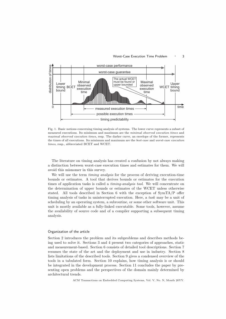
We assume that a real-time system consists of a number of tasks, which realizethe required functionality. Figure 1 depicts several relevant properties of a real-timetask. A task typically shows a certain variation of execution times depending onthe input data or different behavior of the environment. The set of all executiontimes is shown as the upper curve. The shortest execution time is called the best-case execution time (BCET), the longest time is called the worst-case executiontime (WCET). In most cases the state space is too large to exhaustively exploreall possible executions and thereby determine the exact worst-case and best-caseexecution times.

Today, in most parts of industry the common method to estimate execution-time bounds is to measure the end-to-end execution time of the task for a subsetof the possible executions—test cases. This determines the minimal observed andmaximal observed execution times. These will in general overestimate the BCETand underestimate the WCET and so are not safe for hard real-time systems. Thismethod is often called dynamic timing analysis.

Newer measurement-based approaches make more detailed measurements of theexecution time of different parts of the task and combine them to give better esti-mates of the BCET and WCET for the whole task. Still, these methods are rarelyguaranteed to give bounds on the execution time.

Bounds on the execution time of a task can be computed only by methods thatconsider all possible execution times, that is, all possible executions of the task.These methods use abstraction of the task to make timing analysis of the taskfeasible. Abstraction loses information, so the computed WCET bound usuallyoverestimates the exact WCET and vice versa for the BCET. The WCET boundrepresents the worst-case guarantee the method or tool can give. How much islost depends both on the methods used for timing analysis and on overall systemproperties, such as the hardware architecture and characteristics of the software.These system properties can be subsumed under the notion of timing predictability.

The two main criteria for evaluating a method or tool for timing analysis are thussafety—does it produce bounds or estimates?— and precision—are the bounds orestimates close to the exact values?

Performance prediction is also required for application domains that do not havehard real-time characteristics. There, systems may have deadlines, but are not re-quired to absolutely observe them. Different methods may be applied and differentcriteria may be used to measure the quality of methods and tools.

ACM Transactions on Embedded Computing Systems, Vol. V, No. N, Month 20YY.

Worst-Case Execution Time Problem · 3

worst-case performance

dis

trib

ution o

f tim

es

WCETBCET

time

possible execution times

0

Lowertimingbound

Uppertimingbound

timing predictability

worst-case guarantee

Minimalobservedexecution

time

Maximalobservedexecution

time

measured execution times

The actual WCETmust be found orupper bounded

Fig. 1. Basic notions concerning timing analysis of systems. The lower curve represents a subset ofmeasured executions. Its minimum and maximum are the minimal observed execution times andmaximal observed execution times, resp. The darker curve, an envelope of the former, representsthe times of all executions. Its minimum and maximum are the best-case and worst-case executiontimes, resp., abbreviated BCET and WCET.

The literature on timing analysis has created a confusion by not always makinga distinction between worst-case execution times and estimates for them. We willavoid this misnomer in this survey.

We will use the term timing analysis for the process of deriving execution-timebounds or estimates. A tool that derives bounds or estimates for the executiontimes of application tasks is called a timing-analysis tool. We will concentrate onthe determination of upper bounds or estimates of the WCET unless otherwisestated. All tools described in Section 6 with the exception of SymTA/P offertiming analysis of tasks in uninterrupted execution. Here, a task may be a unit ofscheduling by an operating system, a subroutine, or some other software unit. Thisunit is mostly available as a fully-linked executable. Some tools, however, assumethe availability of source code and of a compiler supporting a subsequent timinganalysis.

Organization of the article

Section 2 introduces the problem and its subproblems and describes methods be-ing used to solve it. Sections 3 and 4 present two categories of approaches, staticand measurement-based. Section 6 consists of detailed tool descriptions. Section 7resumes the state of the art and the deployment and use in industry. Section 8lists limitations of the described tools. Section 9 gives a condensed overview of thetools in a tabulated form. Section 10 explains, how timing analysis is or shouldbe integrated in the development process. Section 11 concludes the paper by pre-senting open problems and the perspectives of the domain mainly determined byarchitectural trends.

ACM Transactions on Embedded Computing Systems, Vol. V, No. N, Month 20YY.

4 · Reinhard Wilhelm et al.

2. OVERVIEW OF TIMING-ANALYSIS TECHNIQUES

This section describes the problems that make timing analysis both difficult andinteresting as a research topic, presents a decomposition of the problem into sub-tasks, and categorizes some of the techniques used to determine bounds on executiontimes. A given timing-analysis method or tool may not address or solve all thesesubtasks and different methods and tools may solve the same subtask in differentways.

2.1 Problems and Requirements

Timing analysis attempts to determine bounds on the execution times of a taskwhen executed on a particular hardware. The time for a particular execution de-pends on the path through the task taken by control and the time spent in thestatements or instructions on this path on this hardware. Accordingly, thedetermination of execution-time bounds has to consider the potential control-flowpaths and the execution times for this set of paths. A modular approach to thetiming-analysis problem splits the overall task into a sequence of subtasks. Someof them deal with properties of the control flow, others with the execution time ofinstructions or sequences of instructions on the given hardware.

2.1.1 Data-Dependent Control Flow. The task to be analyzed attains its WCETon one (or sometimes several) of its possible execution paths. If the input and theinitial state leading to the execution of this worst-case path were known, the prob-lem would be easy to solve. The task would then be started in this initial statewith this input, and the execution time would be measured. In general, however,this worst-case input and initial state are not known and hard or impossible to de-termine. A data structure, the task’s control-flow graph, CFG, describes a supersetof the set of all execution paths. The task’s call graph usually is integrated intothe CFG.

A first problem that has to be solved is the construction of the control-flowgraph and call graph of the task from a source or a machine-code version of thetask. They must contain all of the instructions of the task (function closure) underanalysis. Problems are created by dynamic jumps and dynamic calls with computedtarget address. Dynamic jumps are mainly due to switch/case structures and area problem only when analyzing machine code, because even assembly code usuallylabels all switch/case branches. Dynamic calls also occur in source code in the formof calls through function pointers and calls to virtual functions. A component of atiming-analysis tool which reconstructs the CFG from a machine program is oftencalled a Frontend.

Different paths through the CFG are taken depending directly or indirectly oninput data. Some paths in the superset described by the CFG will never be taken,for instance those that have contradictory consecutive conditions. Eliminating suchpaths may increase the precision of timing analysis. The more the analysis knowsabout the data flow through the task, the more it knows about the outcome of andthe relationship between conditions, the more paths it may recognize as infeasible.

A phase called Control-Flow Analysis (CFA) determines information about thepossible flow of control through the task to increase the precision of the subsequentanalyzes. Control flow analysis may attempt to exclude infeasible paths, determine

ACM Transactions on Embedded Computing Systems, Vol. V, No. N, Month 20YY.

Worst-Case Execution Time Problem · 5

execution frequencies of paths or the relation between execution frequencies ofdifferent paths or subpaths etc. Control-Flow Analysis has previously been calledHigh-level Analysis.

Tasks spend most of their execution time in loops and in (recursive) functions.Therefore, it is an essential task of CFA to determine bounds on the iterations ofloops and on the depth of recursion of functions. A necessary ingredient for thisare the values of variables, registers, or memory cells occurring in conditions testedfor termination of loops or recursion.

It is worth noting that complex processors may actually execute an instructionstream in a different order than the one determined by control-flow analysis. Thisis due to pipelining (prefetching and delayed branching), branch prediction, andspeculative or out-of-order execution.

2.1.2 Context Dependence of Execution Times. Early approaches to the timing-analysis problem assumed context independence of the timing behavior; the execu-tion times for individual instructions were independent from the execution historyand could be found in the manual of the processor. From this context independencewas derived a structure-based approach [Shaw 1989]: if a task first executes a codesnippet A and then a snippet B, the worst-case bound for A; B was determined asthat for A, ubA, added to that determined for B, ubB, formally ubA;B = ubA +ubB.This context independence, however, is no longer true for modern processors withcaches and pipelines. The execution time of individual instructions may vary byseveral orders of magnitude depending on the state of the processor in which theyare executed. Thus, the execution time of B can heavily depend on the executionstate that the execution of A produced. Any tool should exploit the knowledge thatA was executed before B to determine a precise upper bound for B in the contextA. Determining the upper bound ubA;B for A; B by ubA;B = ubA + ubB ignoresthis information and will in general not obtain precise results.

A phase called Processor-Behavior Analysis gathers information on the processorbehavior for the given task, in particular the behavior of the components that influ-ence the execution times, such as memory, caches, pipelines, and branch prediction.It determines upper bounds on the execution times of instructions or basic blocks.Processor-Behavior Analysis has previously been called Low-level Analysis.

2.1.3 Timing Anomalies. The complexity of the processor-behavior analysissubtask and the set of applicable methods critically depend on the complexity ofthe processor architecture [Heckmann et al. 2003]. Most powerful microprocessorssuffer from timing anomalies [Lundqvist and Stenstrom 1999c]. Timing anomaliesare contra-intuitive influences of the (local) execution time of one instruction onthe (global) execution time of the whole task. This concept is quite complex. So,we will try to explain it in some detail.

We assume that the system under consideration, executing hardware and ex-ecuted software, are too complex to allow exhaustive execution or simulation. Inaddition, not all input data are known, so that parts of the execution state are miss-ing in the analysis. Unknown parts of the state lead to non-deterministic behavior,if decisions depend on these unknown parts. For timing analysis, this means thatthe execution of an instruction or an instruction sequence considered in an initial

ACM Transactions on Embedded Computing Systems, Vol. V, No. N, Month 20YY.

6 · Reinhard Wilhelm et al.

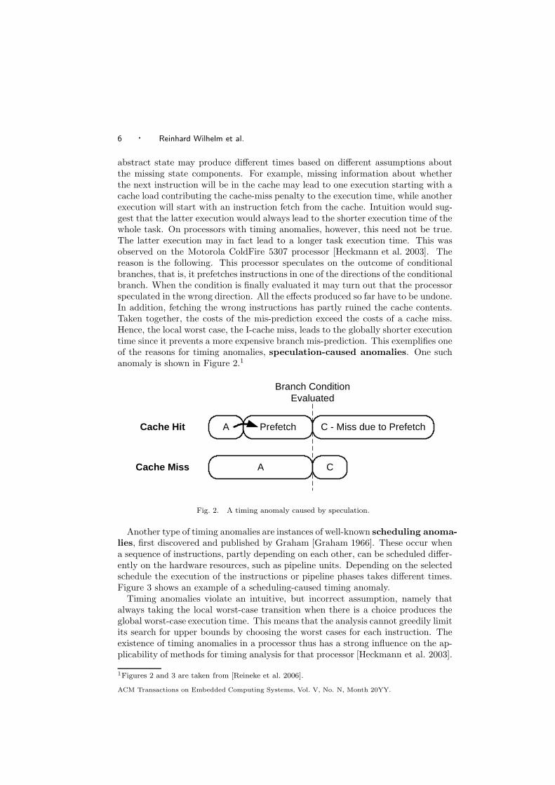
abstract state may produce different times based on different assumptions aboutthe missing state components. For example, missing information about whetherthe next instruction will be in the cache may lead to one execution starting with acache load contributing the cache-miss penalty to the execution time, while anotherexecution will start with an instruction fetch from the cache. Intuition would sug-gest that the latter execution would always lead to the shorter execution time of thewhole task. On processors with timing anomalies, however, this need not be true.The latter execution may in fact lead to a longer task execution time. This wasobserved on the Motorola ColdFire 5307 processor [Heckmann et al. 2003]. Thereason is the following. This processor speculates on the outcome of conditionalbranches, that is, it prefetches instructions in one of the directions of the conditionalbranch. When the condition is finally evaluated it may turn out that the processorspeculated in the wrong direction. All the effects produced so far have to be undone.In addition, fetching the wrong instructions has partly ruined the cache contents.Taken together, the costs of the mis-prediction exceed the costs of a cache miss.Hence, the local worst case, the I-cache miss, leads to the globally shorter executiontime since it prevents a more expensive branch mis-prediction. This exemplifies oneof the reasons for timing anomalies, speculation-caused anomalies. One suchanomaly is shown in Figure 2.1

Prefetch

A

A

Cache Miss

Cache Hit C - Miss due to Prefetch

C

Branch ConditionEvaluated

Fig. 2. A timing anomaly caused by speculation.

Another type of timing anomalies are instances of well-known scheduling anoma-

lies, first discovered and published by Graham [Graham 1966]. These occur whena sequence of instructions, partly depending on each other, can be scheduled differ-ently on the hardware resources, such as pipeline units. Depending on the selectedschedule the execution of the instructions or pipeline phases takes different times.Figure 3 shows an example of a scheduling-caused timing anomaly.

Timing anomalies violate an intuitive, but incorrect assumption, namely thatalways taking the local worst-case transition when there is a choice produces theglobal worst-case execution time. This means that the analysis cannot greedily limitits search for upper bounds by choosing the worst cases for each instruction. Theexistence of timing anomalies in a processor thus has a strong influence on the ap-plicability of methods for timing analysis for that processor [Heckmann et al. 2003].

1Figures 2 and 3 are taken from [Reineke et al. 2006].

ACM Transactions on Embedded Computing Systems, Vol. V, No. N, Month 20YY.

Worst-Case Execution Time Problem · 7

A

A

Resource 1

Resource 2

Resource 1

Resource 2

C

B C

B

D E

D E

Fig. 3. A scheduling-caused timing anomaly.

—The assumption that only local worst cases have to be considered to safely de-termine upper bounds on global execution times is unsafe.

—The assumption that one could identify a worst initial execution state, to safelystart measurement or analysis of a piece of code in, is unsafe.

The consequences for timing analysis of systems to be executed on processorswith timing anomalies are as follows:

—The analysis may be forced to follow execution through several successor states,whenever it encounters an abstract state with a non-deterministic choice betweensuccessor states. This may lead to a quite large state space to consider.

—The analysis has to be able to express the absence of state information instead ofassuming some worst initial state. Absent information in abstract states standsfor all potential concrete instances of these missing state components, thus donot wrongly exclude any possible execution.

2.2 Classification of Approaches

We present two different classes of methods.

Static methods. These methods do not rely on executing code on real hardwareor on a simulator. They rather take the task code itself, maybe together withsome annotations, analyze the set of possible control flow paths through the task,combine control flow with some (abstract) model of the hardware architecture, andobtain upper bounds for this combination. One such static approach is describedin detail in [Wilhelm 2005].

Measurement-based methods. These methods execute the task or task parts onthe given hardware or a simulator for some set of inputs. They then take themeasured times and derive the maximal and minimal observed execution times, seeFigure 1, or their distribution or combine the measured times of code snippets toresults for the whole task.

Static methods emphasize safety by producing bounds on the execution time,guaranteeing that the execution time will not exceed these bounds. The boundsallow safe schedulability analysis of hard real-time systems.

ACM Transactions on Embedded Computing Systems, Vol. V, No. N, Month 20YY.

8 · Reinhard Wilhelm et al.

2.3 Methods for Subtasks of Timing Analysis

We briefly describe some methods that are being used to solve the above mentionedsubtasks of timing analysis. These methods are imported from other fields of com-puter science such as compiler construction, computer architecture, performanceestimation, and optimization.

These methods can be categorized according to several properties: whether theyare automatic or manual, whether they are generic, i.e., stand for a whole class ofmethods, or are specific instances of such a generic method, and whether they areapplied at analysis time or at tool-construction time.

A combination of the methods listed below or instances thereof is required to real-ize a timing analysis method. Several such combinations are described in Sections 3and 4.

2.3.1 Static Program Analysis. Static program analysis is a generic method todetermine properties of the dynamic behavior of a given task without actuallyexecuting the task [Cousot and Cousot 1977; Nielson et al. 1999]. These propertiesare often undecidable. Therefore, sound approximations are used; they have to becorrect, but may not necessarily be complete. An example from our domain isinstruction-cache analysis, which attempts to determine for each point in the taskwhich instructions will be in the cache every time execution reaches this programpoint. For straight-line programs and known initial cache contents this is easy andcan be done by a standard simulator. However, it is in general undecidable fortasks whose control flow depends on input data. A sound analysis will computea subset of the instructions that will definitely be in the instruction cache everytime execution reaches the program point. More instructions may actually be inthe cache, but the analysis may not be able to find this out. Several instances ofstatic program analysis are being used for timing analysis.

2.3.2 Measurement. Measurements can be used in different ways. End-to-endmeasurements of a subset of all possible executions produce estimates, not bounds.They may be useful for applications that do not require guarantees, typically non-hard real-time systems. They may give the developer a feeling about the executiontime in common cases and the likelihood of the occurrence of the worst case. Mea-surement can also be applied to code snippets after which the results are combinedto estimates for the whole program in similar ways as used in static methods. Guar-antees that safe bounds are obtained can currently only be given for rather simplearchitectures due to the reasons given in Section 2.1.

2.3.3 Simulation. Simulation is a standard technique to estimate the executiontime for tasks on hardware architectures. A key advantage of this approach isthat it is possible to derive rather accurate estimations of the execution time fora task for a given set of input data and assuming sufficient detail of the timingmodel of the architectural simulator. However, [Desikan et al. 2001] shows thatnot all simulators can be trusted as clock-cycle accurate simulators for all types ofarchitectures. It compares timing measurements with runs on different simulatorsand gives indication of the errors obtained for an Alpha architecture. The Sim-plescalar [Austin et al. 2002] simulator among others is used. Simplescalar is alsoused by some WCET groups. The results show large differences in timing compared

ACM Transactions on Embedded Computing Systems, Vol. V, No. N, Month 20YY.

Worst-Case Execution Time Problem · 9

to the measured values.

Unfortunately, standard cycle-accurate simulators cannot be used off-hand instatic methods for timing analysis, since static methods should not simulate exe-cution for particular input data, but rather for all input data. Thus, input data isassumed to be unknown. Unknown input data leads to unknown parts in the execu-tion state of the processor and non-deterministic decisions at control-flow branches.Simulators modified to cope with these problems are being used in several of thetools described later.

2.3.4 Abstract Processor Models. Processor-behavior analysis needs a model ofthe architecture. This need not be a concrete model implementing all of the func-tionality of the target hardware. A simplified model that is conservative with re-spect to the timing behavior is sufficient. Such an abstract processor model eitheris a part of the engine for processor-behavior analysis or is input to the constructionof such an engine. In any case, the construction of an abstract processor model isdone at tool-construction time.

One inherent limitation of all the approaches that are based on some model ofthe hardware architecture is that they rely on the timing accuracy of the model.In general, computer vendors do not disclose enough information about the mi-croarchitecture so that one can develop and safely validate the accuracy of a timingmodel. Without such validation, any WCET tool based on an abstract model ofthe hardware cannot be trusted without further assurance. Additional means formodel validation have to be taken. This could be done by measurements. Measuredexecution times are compared against predicted bounds. Another method is tracevalidation checking whether externally observable traces are projections of tracesas predicted by the model. Not all events predicted by the model are externallyobservable. However, both methods are similar to testing; they can discover thepresence of errors, but not prove their absence. Stronger guarantees can be givenby equivalence checking between different abstraction levels. An ongoing researchactivity is the formal derivation of abstract processor models from concrete models.

2.3.5 Integer Linear Programming (ILP). Linear programming [Chvatal 1983]is a generic methodology to code the requirements of a system in the form of asystem of linear constraints. Additionally given is a goal function that has to bemaximized or minimized to obtain an optimal assignment of values to the system’svariables. One speaks of Integer Linear Programming if these values are requiredto be integers. While linear programs can be solved in polynomial time, requiringthe solution to be integer makes the problem NP-hard. This indicates that the useof ILP should be restricted to small problem instances or to subproblems of timinganalysis generating only small problem instances.

In the timing-analysis domain, ILP is used in the IPET approach to boundscalculation, see Section 3.4. The control flow of tasks is translated into integerlinear programs, essentially by coding Kirchhoff’s rule about the conservation offlow. Extra information about the control flow can often be coded as additionalconstraints. The goal function expresses the execution time of the program underanalysis. Its maximal value is then an upper bound for all execution times.

An escape from the exponential complexity that is often taken in other appli-

ACM Transactions on Embedded Computing Systems, Vol. V, No. N, Month 20YY.

10 · Reinhard Wilhelm et al.

cation domains is to use heuristics. These heuristics will in general only arrive atsuboptimal solutions. A suboptimal solution in timing analysis represents an unsafeestimate for the WCET. Thus the escape of resorting to heuristics is barred.

ILP has been used for a completely different purpose, namely to model (very sim-ple) processors [Li et al. 1995b; Li et al. 1995a]. However, the complexity of solvingthe resulting integer linear programs did not allow this approach to scale [Wilhelm 2004].

2.3.6 Annotation. The annotation of tasks with information available from thedeveloper is a generic technique to support subsequently applied automatic vali-dation techniques. The developer using a WCET tool may have to supply someinformation that the tool needs in separate files or by annotating the task. Thisinformation describes

—the memory layout and any needed characteristics of memory areas,

—ranges for the input values of the task,

—information about the control flow of the task if not determined automatically,e.g. loop bounds, shapes of nested loops, if iterations of inner loops depend oniteration variables of outer loops, frequencies of paths or branches taken,

—deviations from the standard function-calling conventions, and

—directives as to the desired precision of the result, which often depends on theinvested effort for differentiating contexts.

2.3.7 Frontend. Most WCET tools analyze software at the executable level,since only at this level is all necessary information available. The first phase intiming analysis is thus the decoding of the executable and the reconstruction of itscontrol flow. This can be quite involved depending on the instruction set of theprocessor and the code-generation patterns of the compiler. Some timing analysistools are integrated with a compiler which emits the necessary CFG and call graphfor the analysis.

2.3.8 Visualization of Results. The results of timing analysis are presented inhuman-readable form, best in the form of an informative visualization. This usuallyshows the call and control-flow graphs annotated with computed timing informationand possibly also information about the processor states.

The following two sections present the two categories of approaches, static andmeasurement-based approaches. Section 6 describes the available tools from thesetwo categories in more detail.

3. STATIC METHODS

This class of methods does not rely on executing code on real hardware or on asimulator, but rather takes the task code itself, combines it with some (abstract)model of the system, and obtains upper bounds from this combination.

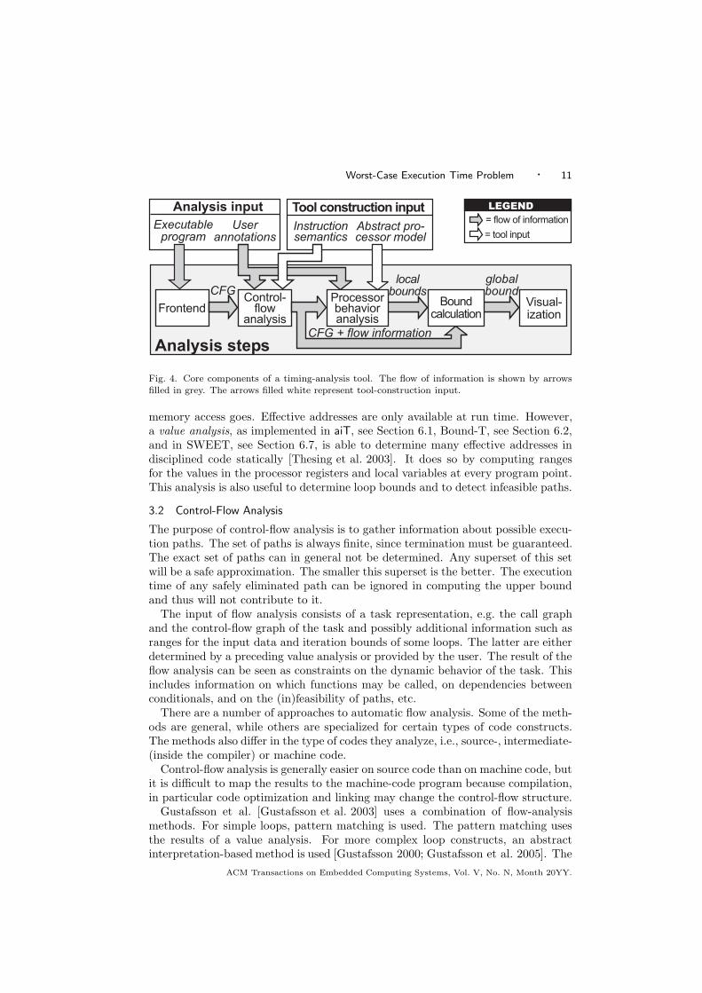
Figure 4 shows the core components of a static timing-analysis tool and the flowof information.

3.1 Value Analysis

This is a static program analysis. Any method for data-cache behavior analysisneeds to know effective memory addresses of data, in order to determine where a

ACM Transactions on Embedded Computing Systems, Vol. V, No. N, Month 20YY.

Worst-Case Execution Time Problem · 11

Userannotations

Visual-ization

localbounds

globalbound

Analysis input

Control-flow

analysisFrontend

CFG

CFG + flow information

Executableprogram

Boundcalculation

Analysis steps

Processorbehavioranalysis

Abstract pro-cessor model

Tool construction input

Instructionsemantics

LEGEND

= flow of information

= tool input

Fig. 4. Core components of a timing-analysis tool. The flow of information is shown by arrowsfilled in grey. The arrows filled white represent tool-construction input.

memory access goes. Effective addresses are only available at run time. However,a value analysis, as implemented in aiT, see Section 6.1, Bound-T, see Section 6.2,and in SWEET, see Section 6.7, is able to determine many effective addresses indisciplined code statically [Thesing et al. 2003]. It does so by computing rangesfor the values in the processor registers and local variables at every program point.This analysis is also useful to determine loop bounds and to detect infeasible paths.

3.2 Control-Flow Analysis

The purpose of control-flow analysis is to gather information about possible execu-tion paths. The set of paths is always finite, since termination must be guaranteed.The exact set of paths can in general not be determined. Any superset of this setwill be a safe approximation. The smaller this superset is the better. The executiontime of any safely eliminated path can be ignored in computing the upper boundand thus will not contribute to it.

The input of flow analysis consists of a task representation, e.g. the call graphand the control-flow graph of the task and possibly additional information such asranges for the input data and iteration bounds of some loops. The latter are eitherdetermined by a preceding value analysis or provided by the user. The result of theflow analysis can be seen as constraints on the dynamic behavior of the task. Thisincludes information on which functions may be called, on dependencies betweenconditionals, and on the (in)feasibility of paths, etc.

There are a number of approaches to automatic flow analysis. Some of the meth-ods are general, while others are specialized for certain types of code constructs.The methods also differ in the type of codes they analyze, i.e., source-, intermediate-(inside the compiler) or machine code.

Control-flow analysis is generally easier on source code than on machine code, butit is difficult to map the results to the machine-code program because compilation,in particular code optimization and linking may change the control-flow structure.

Gustafsson et al. [Gustafsson et al. 2003] uses a combination of flow-analysismethods. For simple loops, pattern matching is used. The pattern matching usesthe results of a value analysis. For more complex loop constructs, an abstractinterpretation-based method is used [Gustafsson 2000; Gustafsson et al. 2005]. The

ACM Transactions on Embedded Computing Systems, Vol. V, No. N, Month 20YY.

12 · Reinhard Wilhelm et al.

analysis is performed on the intermediate code level. Pattern-matching methodsare based on the fact that for most loops the supported compilers use the same orsimilar groups of machine instructions to initialize, update and test loop counters.Pattern-matching finds occurrences of such instruction groups in the code and an-alyzes the values of the instruction operands to find the counter range, for examplein terms of the initial value, the increment or decrement and the final value ofthe counter. The drawback of this method is that it can be defeated by compileroptimizations, or by evolution of the compiler itself, if this changes the emittedinstruction patterns so much that the matching fails.

Bound-T, see Section 6.2, finds loop bounds by modelling the computation, in-struction by instruction, using affine equations and inequalities (Presburger Arith-metic). Bound-T then examines the model to find variables that act as loop coun-ters. If Bound-T also finds bounds on the initial and final values of the variable, asimple computation gives a bound on the number of loop iterations.

Whalley et al. [Healy et al. 1998; Healy and Whalley 1999] use data flow analysisand special algorithms to calculate bounds for single and nested loops in conjunc-tion with a compiler. [Stappert and Altenbernd 2000] uses symbolic execution onthe source code level to derive flow information. aiT’s loop-bound analysis, seeSection 6.1, is based on a combination of an interval-based abstract interpretationand pattern-matching [Thesing 2004] working on the machine code.

The result of control-flow analysis is an annotated syntax tree for the structure-based approaches, see Section 3.4, and a set of flow facts about the transitions ofthe control-flow graph, otherwise. These flow facts are translated into a system ofconstraints for the methods using implicit path enumeration, see Section 3.4.

3.3 Processor-Behavior Analysis

As stated in Section 2.1.2, a typical processor contains several components thatmake the execution time context-dependent, such as memory, caches, pipelines andbranch prediction. The execution time of an individual instruction, even a memoryaccess depends on the execution history. To find precise execution-time bounds fora given task, it is necessary to analyze what the occupancy state of these processorcomponents for all paths leading to the task’s instructions is. Processor-behavioranalysis determines invariants about these occupancy states for the given task.In principle, no tool is complete that does not take the processor periphery intoaccount, i.e., the full memory hierarchy, the bus, and peripheral units. In so far, aneven better term would be hardware-subsystem behavior analysis. The analysis isdone on a linked executable, since only this contains all the necessary information.It is based on an abstract model of the processor, the memory subsystem, the buses,and the peripherals, which is conservative with respect to the timing behavior ofthe concrete hardware, i.e., it never predicts an execution time less than that whichcan be observed on the concrete processor.

The complexity of deriving an abstract processor model strongly depends on theclass of processor used.

—For simpler 8bit and 16bit processors the timing model construction is rathersimple, but still time consuming, and rather simple analyses are required. Com-plicating factors for the processor behavior analysis include instructions with

ACM Transactions on Embedded Computing Systems, Vol. V, No. N, Month 20YY.

Worst-Case Execution Time Problem · 13

varying execution time due to argument values and varying data reference timedue to different memory area access times.

—For somewhat more advanced 16bit and 32bit processors, like the NEC V850E,possessing a simple (scalar) pipeline and maybe a cache, one can analyze differ-ent hardware features separately, since there are no timing anomalies, and stillachieve good results. Complicating factors are similar as for the simpler 8- and16-bit processors, but also include varying access times due to cache hits andmisses and varying pipeline overlap between instructions.

—More advanced processors, which possess many performance enhancing featuresthat can influence each other, will exhibit timing anomalies. For these, timing-model construction is very complex. Also the analyses to be used are less modularand more complex [Heckmann et al. 2003].

In general, the execution-time bounds derived for an instruction depend on thestates of the processor at this instruction. Information about the processor statesis derived by analyzing potential execution histories leading to this instruction.Different states in which the instruction can be executed may lead to widely varyingexecution times with disastrous effects on precision. For instance, if a loop iterates100 times, but the worst case of the body, ebody, only really occurs during one ofthese iterations and the others are considerably faster (say twice as fast), the over-approximation is 99∗ 0.5 ∗ ebody. Precision can be gained by regarding execution inclasses of execution histories separately, which correspond to flow contexts. Theseflow contexts essentially express by which paths through loops and calls control canarrive at the instruction. Wherever information about the processor’s executionstate is missing a conservative assumption has to be made or all possibilities haveto be explored.

Most approaches use Data Flow Analysis, a static program-analysis techniquebased on the theory of Abstract Interpretation [Cousot and Cousot 1977]. Thesemethods are used to compute invariants, one per flow context, about the proces-sor’s execution states at each program point. If there is one invariant for eachprogram point, then it holds for all execution paths leading to this program point.Different ways to reach a basic block may lead to different invariants at the block’sprogram points. Thus, several invariants could be computed. Each holds for a setof execution paths, and the sets together form a partition of the set of all execu-tion paths leading to this program point. Each set of such paths corresponds towhat sometimes is called a calling context, context for short. The invariants ex-press static knowledge about the contents of caches, the occupancy of functionalunits and processor queues, and of states of branch-prediction units. Knowledgeabout cache contents is then used to classify memory accesses as definite cachehits (or definite cache misses). Knowledge about the occupancy of pipeline queuesand functional units is used to exclude pipeline stalls. Assume that one uses thefollowing method: First accept Murphy’s Law, that everything that can go wrong,actually goes wrong, assuming worst cases all over. Then both types of “goodnews” of the type described above can often be used to reduce the upper boundsfor the execution times. Unfortunately, this approach is not safe for many processorarchitectures with timing anomalies, see Section 2.1.3.

ACM Transactions on Embedded Computing Systems, Vol. V, No. N, Month 20YY.

14 · Reinhard Wilhelm et al.

3.4 Estimate Calculation

The purpose is to determine an estimate for the WCET. In dynamic approaches theWCET estimate can underestimate the WCET, since only a subset of all executionsis used to compute it. Combining measurements of code snippets to end-to-endexecution times can also overestimate the WCET, if pessimistic estimates for thesnippets are combined. In static approaches this phase computes an upper boundof all execution times of the whole task based on the flow and timing informationderived in the previous phases. It is then usually called Bound Calculation. Thereare three main classes of methods combining analytically determined or measuredtimes to end-to-end estimates proposed in literature: structure-based, path-based,and techniques using implicit path enumeration (IPET).

Fig. 5 taken from [Ermedahl 2003] shows the different methods. Fig. 5(a) showsan example control-flow graph with timing on the nodes and a loop-bound flowfact.

In structure-based bound calculation as used in Heptane, cf. [Colin and Puaut 2000]and Section 6.6, an upper bound is calculated in a bottom-up traversal of the syn-tax tree of the task combining bounds computed for constituents of statementsaccording to combination rules for that type of statement [Colin and Bernat 2002;Colin and Puaut 2000; Lim et al. 1995]. Fig. 5(d) illustrates how a structure-basedmethod would proceed according to the task syntax tree and given combinationrules. Collections of nodes are collapsed into single nodes, simultaneously deriv-ing a timing for the new node. As stated in Section 2.1.2, precision can only beobtained if the same code snippet is considered in a number of different flow con-texts, since the execution times in different flow contexts can vary widely. Takingflow contexts into account requires transformations of the syntax tree to reflect thedifferent contexts. Most of the profitable transformations, e.g. loop unrolling, areeasily expressed on the syntax tree [Colin and Bernat 2002].

Some problems of the structure-based approach are that not every control flowcan be expressed through the syntax tree, that the approach assumes a very straight-forward correspondence between the structures of the source and the target programnot easily admitting code optimizations, and that it is in general not possible toadd additional flow information as can be done in the IPET case.

In path-based bound calculation, the upper bound for a task is determined bycomputing bounds for different paths in the task, searching for the overall pathwith the longest execution time [Healy et al. 1999; Stappert and Altenbernd 2000;Stappert et al. 2001]. The defining feature is that possible execution paths arerepresented explicitly. The path-based approach is natural within a single loopiteration, but has problems with flow information extending across loop-nestinglevels. The number of paths is exponential in the number of branch points, possiblyrequiring heuristic search methods.

Fig. 5(b) illustrates how a path-based calculation method would proceed overthe graph in Fig. 5(a). The loop in the graph is first identified and the longestpath within the loop is found. The time for the longest path is combined with flowinformation about the loop bound to extract an upper bound for the whole task.

In IPET, program flow and basic-block execution time bounds are combined intosets of arithmetic constraints. The idea was originally proposed in [Li and Malik 1995]

ACM Transactions on Embedded Computing Systems, Vol. V, No. N, Month 20YY.

Worst-Case Execution Time Problem · 15

and adapted to more complex flows and hardware timing effects in [Puschner and Schedl 1995;Engblom 2002; Theiling 2002a; Theiling 2002b; Ermedahl 2003]. Each basic blockand program flow edge in the task is given a time coefficient (tentity ), expressingthe upper bound of the contribution of that entity to the total execution time everytime it is executed and a count variable (xentity ), corresponding to the number oftimes the entity is executed. An upper bound is determined by maximizing thesum of products of the execution counts and times (

∑i∈entities

xi ∗ ti), where theexecution count variables are subject to constraints reflecting the structure of thetask and possible flows. The result of an IPET calculation is an upper timing boundand a worst-case count for each execution count variable.

exit

start

H

A3

12

2

B,C,D

E,F,G 14

(a) Control-flowgraph with timing

B

E

DC

exit

start

H

GF

A3

5

47

6

58

2

3

5

47

6

58

2

B

E

DC

exit

start

H

GF

A

maxiter:100

// WCET CalcWCET =

theader + tpath *

(maxiter-1) =3 + 31 * 99 =3072

// Unit timingtpath = 31theader = 3

(b) Path-based calculation

Longest pathmarked

T(seq(S1,S2)) = T(S1) +T(S2)

T(if(Exp) S1 else S2) = T(Exp) + max(T(S1),T(S2))

T(loop(Exp,Body)) = T(Exp) + (T(Exp) +T(Body)) * (maxiter-1)

Transformation rules (d) Structure-based calculation

exit

start

A3

28B,C,D,E,F,G,H

FinalProgramWCET

if seq loop

B

E

DC

exit

start

H

GF

A3

5

47

6

58

2

exit

start

3072

A,B,C,DE,F,G,H

B

E

DC

exit

start

H

GF

A xA

xAB

xB

xstart xHA

xBC xBD

xEF xEG

xE

xC xD

xF xG

xCE xDE

xFH xGH

xH

xexit

xstartA

xAexit

// Start and exit constraintsxstart = 1, xexit = 1

// Structural constraintsxstart = xstartAxA = xstartA + xHA = xAexit + xABxB = xAB = xBC + xBDxC = xBC = xCE

. . .

xH = xFH + xGH = xHAxexit = xAexit

// Loopbound constraintxA £ 100

// WCET ExpressionWCET = max(xA*3 + xB*5 + xC*7 + ... + xH*2) = = 3072

(c) IPET calculation

loop

seq

seqif

A

B C D if

E F G

H

Syntax-tree

Fig. 5. Bound calculation

Fig. 5(c) shows the constraints and formulae generated by an IPET-based bound-calculation method for the task illustrated in Fig. 5(a). The start and exit con-straints state that the task must be started and exited once. The structural con-straints reflect the possible program flow, meaning that for a basic block to beexecuted it must be entered the same number of times as it is exited. The loopbound is specified as a constraint on the number of times the loop-head node A canbe executed.

ACM Transactions on Embedded Computing Systems, Vol. V, No. N, Month 20YY.

16 · Reinhard Wilhelm et al.

IPET is able to handle different types of flow information. It has traditionallybeen applied in a global fashion treating the whole task and all flow informationtogether as a unit. IPET-based bound calculation uses integer linear program-ming (ILP) or constraint programming (CP) techniques, thus having a complexitypotentially exponential in the task size. Also, since flow facts are converted to con-straints, the size of the resulting constraint system grows with the number of flowfacts.

3.5 Symbolic Simulation

Another static method is to simulate the execution of the task in an abstract modelof the processor. The simulation is performed without input. The simulator thushas to be capable to deal with partly unknown execution state. This methodcombines flow analysis, processor-behavior prediction, and bound calculation in oneintegrated phase [Lundqvist 2002]. One problem with this approach is that analysistime is proportional to the actual execution time of the task. This can lead to avery long analysis since simulation is typically orders of magnitudes slower thannative execution.

4. MEASUREMENT-BASED METHODS

These methods attack some parts of the timing-analysis problem by executing thegiven task on the given hardware or a simulator, for some set of inputs, and mea-suring the execution time of the task or its parts.

End-to-end measurements of a subset of all possible executions produce estimatesor distributions, not bounds for the execution times, if the subset is not guaranteedto contain the worst case. Even one execution would be enough if the worst-caseinput were known.

Other approaches measure the execution times of code segments, typically ofCFG basic blocks. The measured execution times are then combined and analyzed,usually by some form of bound calculation, to produce estimates of the WCET orBCET. Thus, measurement replaces the processor-behaviour analysis used in staticmethods. Thus, the path-subset problem can be solved in the same way as forthe static methods, using control flow analysis to find all possible paths and thenusing bound calculation to combine the measured times of the code segments intoan overall time bound. This solution would include all possible paths, but wouldstill produce unsafe results if the measured basic-block times were unsafe. Anotherproblem is that only a subset of the possible contexts (initial processor states) isused for each measured basic block or other kind of code segment.

The context-subset problem could be attacked by running more tests to measuremore contexts or by setting up a worst-case initial state at the start of each measuredcode segment. The first method (more tests) only decreases, but does not eliminatethe risk of unsafe results and is expensive unless intensive testing is already done forother reasons. Exhaustive testing of all execution paths is usually impossible. Thesecond method (use worst-case initial state) would be safe if one could determinea worst-case initial state. However, identifying worst-case initial states is hard oreven impossible for complex processors, see below. Measurement-based tools cancompute execution-time bounds for processors with simple timing behaviour, butproduce only estimates of the BCET and WCET for more complex processors, as

ACM Transactions on Embedded Computing Systems, Vol. V, No. N, Month 20YY.

Worst-Case Execution Time Problem · 17

long as this problem is not convincingly solved. Other tools collect and analysemultiple measurements to provide a picture of the variability of the execution timeof the application, in addition to estimates of the BCET and WCET.

There are multiple ways in which measurement can be performed. The simplestapproach is by extra instrumentation code that collects a timestamp or CPU cyclecounter (available in most processors). Mixed HW/SW instrumentation techniquesrequire external hardware to collect timings of lightweight instrumentation code.Fully transparent (non-intrusive) measurement mechanisms are possible using logicanalyzers. Also hardware tracing mechanisms like the NEXUS standard and theETM tracing mechanism from ARM are non-intrusive, but don’t necessarily pro-duce exact timings. For example, NEXUS buffers its output, and time stamps areproduced when events leave the buffer, i.e. with a delay. Measurements can alsobe performed from the output of processor simulators or even VHDL simulators.

The results of measurement-based analysis can be used to provide a picture ofthe actual variability of the execution time of the application. They can also beused to provide validation for the static analyis approaches. Measurement shouldalso not produce execution times that are far lower than the ones predicted byanalytical methods, because this would indicate that the latter are imprecise.

5. COMPARISON OF STATIC AND MEASUREMENT-BASED METHODS

In this section, we attempt to compare the two classes of timing-analysis methods—static and measurement-based—to highlight the differences and similarities in theiraims, abilities, technical problems and research directions. The next section willdescribe some timing-analysis tools in more detail to show the state of the practiceof both classes of methods.

Static methods compute bounds on the execution time. They use control-flowanalysis and bound calculation to cover all possible execution paths. They useabstraction to cover all possible context dependencies in the processor behaviour.The price they pay for this safety is the necessity for processor-specific models ofprocessor behaviour, and possibly imprecise results such as overestimated WCETbounds. In favour of static methods is the fact that the analysis can be done withoutrunning the program to be analysed—which often needs complex equipment tosimulate the hardware and peripherals of the target system.

Measurement-based methods replace processor behaviour analysis by measure-ments. Therefore, unless all possible execution paths are measured or the processoris simple enough to let each measurement be started in a worst-case initial state,some context-dependent execution-time changes may be missed and the methodis unsafe. For the estimate-calculation step, these methods may use control-flowanalysis to include all possible execution paths, or they may simply use the ob-served execution paths (observed number of loop iterations, for example) whichagain makes the method unsafe. The advantages claimed for these methods arethat they are simpler to apply to new target processors, because they do not needto model processor behaviour, and that they produce WCET and BCET estimatesthat are more precise—closer to the exact WCET and BCET—than the boundsfrom static methods, especially for complex processors and complex applications.

Still, since the exact WCET or BCET is usually not known, there is really no way

ACM Transactions on Embedded Computing Systems, Vol. V, No. N, Month 20YY.

18 · Reinhard Wilhelm et al.

to check how precise an estimate or bound is. Studies of precision often comparethe estimates or bounds not to the exact WCET or BCET but to the extremeobserved times from a large but not exhaustive set of tests.

Users can help to improve precision for both classes of methods. For the staticmethods, users can improve the precision (tighten the bounds) by annotations thatexclude infeasible executions from the analysis. For the measurement-based meth-ods, users can improve the precision by adding test cases to include more possibleexecutions in the measurements. Some measurement-based tools also allow anno-tations for the estimate calculation to exclude infeasible executions or to includemore executions by defining larger loop bounds than have been observed.

Both classes of methods share some technical problems and solutions. The front-ends are similar when both use executable code as input; control-flow analysis issimilar; and bound/estimate calculation can be similar. For example, the IPETcalculation is used by some static tools and by some measurement-based tools.

The main technical problem for static methods is modelling processor behaviour.This is not a problem for most measurement-based methods, where the main prob-lem is to measure the execution time accurately, with fine granularity, and with-out perturbing the program being measured. The solution is often processor- orplatform-specific, but implementing a measurement method for a new processor isusually less work than creating an abstract model of the processor behaviour.

The handling of timing anomalies offers an interesting comparison of the methods.For measurement-based methods, timing anomalies make it very hard to find aworst-case initial state for a measurement. To be safe, the measurement shouldnow be done from all possible initial states, which is impractical. Measurement-based methods then use only a subset of initial states and so are not safe.

Static methods based on abstract interpretation have ways to express the absenceof information and can therefore analyse large state sets, including all possiblestates for a safe analysis. Here, timing anomalies make it hard to define stateabstractions that give a precise abstract interpretation of each instruction and of theexecution time spent in the instruction—the processor behaviour tends to dependon unknown aspects of the state, forcing the abstract simulation to follow manypossible executions of each basic block. Still, this laborious exploration is limitedto basic blocks, because the abstract simulation considers the global flow of thetask for the processor-behavior analysis by propagating simulation results betweenbasic blocks. Thus, no worst case assumptions need to be made by the analysis onthe basic block level.

Current research in these methods addresses some shared problems, while eachclass of methods also has its own research directions. Clearly, research into im-proved abstract processor models is relevant only to static methods, while the de-velopment of better measurement methods—in particular, standard interfaces formeasurement for many processor types—is of interest mainly for the measurement-based methods.

Control-flow analysis, on the other hand, is a common subject of research thatapplies to both static methods and measurement-based meethods. Another com-mon subject is the separation of contexts to improve the precision of the analysis.This means that a given part of the task under analysis, for example a subroutine or

ACM Transactions on Embedded Computing Systems, Vol. V, No. N, Month 20YY.

Worst-Case Execution Time Problem · 19

a loop body, can be analysed or measured separately depending on its context, forexample the call-path to the subroutine, or the ieration number of the loop. Here,the question that is common to static methods and measurement-based methods iswhen to separate between contexts and how—automatically or by manual annota-tions.

6. COMMERCIAL WCET TOOLS AND RESEARCH PROTOTYPES

The tool providers and researchers participating in this survey have received thefollowing list of questions:

—What is the functionality of your tool?

—What methods are employed in your tool?

—What are the limitations of your tool?

—Which hardware platforms does your tool support?

This section has the following line-up of tools, from completely static tools suchas aiT in Subsection 6.1, Bound-T in Subsection 6.2, and the prototypes of Florida(Subsection 6.3), Vienna (Subsection 6.4), Singapore (Subsection 6.5), and IRISA(Subsection 6.6), through mostly static tool with a small rudiment of measurementin SWEET (very controlled pipeline measurements on a simulator), in Subsec-tion 6.7, and the Chalmers prototype (Subsection 6.8), through SymTA/P (cacheanalysis and block/segment measurement starting from a controlled cache stateand bound calculation), in Subsection 6.9, to the most measurement-based tool,RapiTime (block measurement from an uncontrolled initial state and bound calcu-lation), in Subsection 6.10.

6.1 The aiT Tool of AbsInt Angewandte Informatik, Saarbrucken, Germany

Functionality of the Tool. The purpose of AbsInt’s timing-analysis tool aiT isto obtain upper bounds for the execution times of code snippets (e.g. given assubroutines) in executables. These code snippets may be tasks called by a schedulerin some real-time application, where each task has a specified deadline. aiT workson executables because the source code does not contain information on registerusage and on instruction and data addresses. Such addresses are important forcache analysis and the timing of memory accesses in case there are several memoryareas with different timing behavior.

Apart from the executable, aiT might need user input to be able to compute aresult or to improve the precision of the result. User annotations may be writteninto parameter files and refer to program points by absolute addresses, addressesrelative to routine entries, or structural descriptions (like the first loop in a routine).Alternatively, they can be embedded into the source code as special comments. Inthat case, they are mapped to binary addresses using the line information in theexecutable.

Apart from the usual user annotations (loop bounds, flow facts), aiT supportsannotations specifying the values of registers and variables. The latter is useful foranalyzing software running in several different modes that are distinguished by thevalue of a mode variable.

ACM Transactions on Embedded Computing Systems, Vol. V, No. N, Month 20YY.

20 · Reinhard Wilhelm et al.

Fig. 6. Architecture of the aiT WCET analysis tool

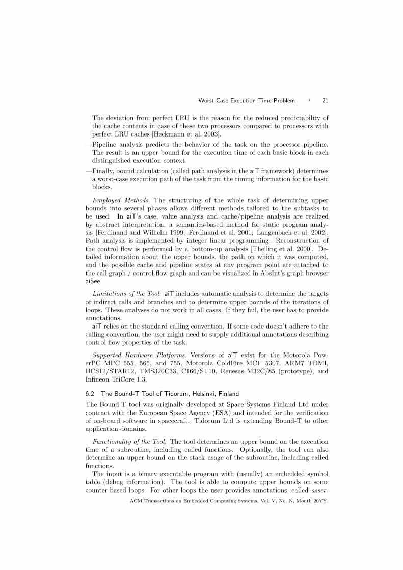
The aiT versions for all supported processors share a common architecture asshown in Fig. 6:

—First, the control flow is reconstructed from the given object code by a bot-tom up approach. The reconstructed control flow is annotated with the infor-mation needed by subsequent analyses and then translated into CRL (ControlFlow Representation Language, a human-readable intermediate format designedto simplify analysis and optimization at the executable/assembly level). Thisannotated control-flow graph serves as the input for the following analysis steps.

—Next, value analysis computes ranges for the values in the processor registersat every program point. Its results are used for loop bound analysis, for thedetection of infeasible paths depending on static data, and to determine possibleaddresses of indirect memory accesses. An extreme case of control depending onstatic data is a virtual machine program interpreting abstract code given as data.[Souyris et al. 2005] report on a successful analysis of such an abstract machine.

—aiT’s cache analysis relies on the addresses of memory accesses as found by valueanalysis and classifies memory references as sure hits and potential misses. It isbased upon [Ferdinand and Wilhelm 1999], which handles LRU caches, but hadto be modified to reflect the non-LRU replacement strategies of common mi-croprocessors: the pseudo-round-robin replacement policy of the ColdFire MCF5307, and the PLRU (Pseudo-LRU) strategy of the PowerPC MPC 750 and 755.

ACM Transactions on Embedded Computing Systems, Vol. V, No. N, Month 20YY.

Worst-Case Execution Time Problem · 21

The deviation from perfect LRU is the reason for the reduced predictability ofthe cache contents in case of these two processors compared to processors withperfect LRU caches [Heckmann et al. 2003].

—Pipeline analysis predicts the behavior of the task on the processor pipeline.The result is an upper bound for the execution time of each basic block in eachdistinguished execution context.

—Finally, bound calculation (called path analysis in the aiT framework) determinesa worst-case execution path of the task from the timing information for the basicblocks.

Employed Methods. The structuring of the whole task of determining upperbounds into several phases allows different methods tailored to the subtasks tobe used. In aiT’s case, value analysis and cache/pipeline analysis are realizedby abstract interpretation, a semantics-based method for static program analy-sis [Ferdinand and Wilhelm 1999; Ferdinand et al. 2001; Langenbach et al. 2002].Path analysis is implemented by integer linear programming. Reconstruction ofthe control flow is performed by a bottom-up analysis [Theiling et al. 2000]. De-tailed information about the upper bounds, the path on which it was computed,and the possible cache and pipeline states at any program point are attached tothe call graph / control-flow graph and can be visualized in AbsInt’s graph browseraiSee.

Limitations of the Tool. aiT includes automatic analysis to determine the targetsof indirect calls and branches and to determine upper bounds of the iterations ofloops. These analyses do not work in all cases. If they fail, the user has to provideannotations.

aiT relies on the standard calling convention. If some code doesn’t adhere to thecalling convention, the user might need to supply additional annotations describingcontrol flow properties of the task.

Supported Hardware Platforms. Versions of aiT exist for the Motorola Pow-erPC MPC 555, 565, and 755, Motorola ColdFire MCF 5307, ARM7 TDMI,HCS12/STAR12, TMS320C33, C166/ST10, Renesas M32C/85 (prototype), andInfineon TriCore 1.3.

6.2 The Bound-T Tool of Tidorum, Helsinki, Finland

The Bound-T tool was originally developed at Space Systems Finland Ltd undercontract with the European Space Agency (ESA) and intended for the verificationof on-board software in spacecraft. Tidorum Ltd is extending Bound-T to otherapplication domains.

Functionality of the Tool. The tool determines an upper bound on the executiontime of a subroutine, including called functions. Optionally, the tool can alsodetermine an upper bound on the stack usage of the subroutine, including calledfunctions.

The input is a binary executable program with (usually) an embedded symboltable (debug information). The tool is able to compute upper bounds on somecounter-based loops. For other loops the user provides annotations, called asser-

ACM Transactions on Embedded Computing Systems, Vol. V, No. N, Month 20YY.

22 · Reinhard Wilhelm et al.

tions in Bound-T. Annotations can also be given for variable values to support theautomatic loop-bounding.

The output is a text file listing the upper bounds etc. and graph files showing call-graphs and control-flow graphs for display with the DOT tool [Gansner and North 2000].

As a further option, when the task under analysis follows the ESA-specifiedHRT (“Hard Real Time”) tasking architecture, Bound-T can generate the HRTExecution Skeleton File that contains both the tasking structure and the computedbounds and can be fed directly into the ESA-developed tools for SchedulabilityAnalysis and Scheduling Simulation.

Employed Methods. Reading and decoding instructions is hand-coded based onprocessor manuals. The processor model is also manually constructed for eachprocessor. Bound-T has general facilities for modelling control flow and integerarithmetic, but not for modelling complex processor states. Some special-purposestatic analyses have been implemented, for example for the SPARC register-fileoverflow and underflow traps and for the concurrent operation of the SPARC IntegerUnit and Floating Point Unit. Both examples use (simple) abstract interpretationfollowed by ILP.

The control-flow graph (CFG) is often defined to model the processor’s instruction-sequencing behaviour, not just the values of the program counter. A CFG nodetypically represents a certain pipeline state, so the CFG is really a pipeline-stategraph. Instruction interactions (e.g. data-path blocking) are modelled in the timeassigned to CFG edges.

Counter-based loops are bounded by modelling the task’s loop-counter arith-metic as follows. The computational effect of each instruction is modelled as arelation between the ”before” and ”after” values of the variables (registers andother storage locations). The relation is expressed in Presburger Arithmetic as aset of affine (linear plus constant term) equations and inequalities, possibly condi-tional. Instruction sequences are modelled by concatenating (joining) the relationsof individual instructions. Branching control-flow is modelled by adding the branchcondition to the relation. Merging control-flow is modelled by taking the union ofthe inflowing relations.

Loops are modelled by analysing the model of the loop-body to classify variablesas loop-invariant or loop-variant. The whole loop (including an unknown numberof repetitions) is modelled as a relation that keeps the loop-invariant variablesunchanged and assigns unknown values to the loop-variant variables. This is afirst approximation that may be improved later in the analysis when the numberof loop iterations is bounded. With this approximation, the computations in anentire subprogram can be modelled in one pass (without fixpoint iteration).

To bound loop iterations, Bound-T first re-analyses the model of the loop body inmore detail to find loop-counter variables. A loop counter is a loop-variant variablesuch that one execution of the loop body changes the variable by an amount thatis bounded to a finite interval that does not contain zero. If Bound-T also findsbounds on the initial and final values of the variable, a simple computation gives abound on the number of loop iterations.

Bound-T uses the Omega Calculator from Maryland University [Pugh 1991] tocreate and analyze the equation set. Loop-bounds can be context-dependent if they

ACM Transactions on Embedded Computing Systems, Vol. V, No. N, Month 20YY.

Worst-Case Execution Time Problem · 23

depend on scalar pass-by-value parameters for which actual values are provided atthe top (caller end) of a call-path.

The worst-case path and the upper bound for one subroutine are found by theImplicit Path Enumeration Technique, (see Section 3.4) applied to the control-flowgraph of the subroutine. The lp solve tool is used [Berkelaar 1997]. If the subroutinehas context-dependent loop bounds, the IPET solution is computed separately foreach context (call path).

Annotations are written in a separate text file, not embedded in source-code. Theprogram element to which an annotation refers is identified by a symbolic name(subroutine, variable) or by structural properties (loops, calls). The structuralproperties include nesting of loops, location of calls with respect to loops, andlocation of variable reads and writes.

Limitations of the Tool. The task to be analyzed must not be recursive. Thecontrol-flow graphs must be reducible. Dynamic (indexed) calls are only analyzedin special cases, when Bound-T’s data-flow analysis finds a unique target address.Dynamic (indexed) jumps are analyzed based on the code patterns that the sup-ported compilers generate for switch/case structures, but not all such structuresare supported.

Bound-T can detect some infeasible paths as a side-effect of its loop-bound anal-ysis. There is, however, no systematic search for such paths. Points-to analysis(aliasing analysis) is weak, which is a risk for the correctness of the loop-boundanalysis.

The bounds of an inner loop cannot depend on the index of the outer loop(s).For such “non-rectangular” loops Bound-T can often produce a “rectangular” upperbound. Loop-bound analysis does not cover the operations of multiplication (exceptby a constant), division or the logical bit-wise operations (and, or, shift, rotate).

The task to be analyzed must use the standard calling conventions. Furthermore,function pointers are not supported in general, although some special cases such asstatically assigned interrupt vectors can be analyzed.

No cache analysis is yet implemented (the current target processors have no cacheor very small and special caches). Any timing anomalies in the target processormust be taken into account in the execution time that is assigned to each basic blockin the CFG. However, the currently supported, cacheless processors probably haveno timing anomalies. As Bound-T has no general formalism (beyond the CFG) formodelling processor state, it has no general limitations in that regard, but modelsfor complex processors would be correspondingly harder to implement in Bound-T.

Supported Hardware Platforms. Intel-8051 series (MCS-51), Analog Devices ADSP-21020, ATMEL ERC32 (SPARC V7), Renesas H8/300, ARM7 (prototype) andATMEL AVR and ATmega (prototypes).

6.3 Research Prototype from Florida State University, North Carolina State University,Furman University

The main application areas for our timing analysis tools are hard real-time systemsand energy-aware embedded systems with timing constraints. We are currentlyworking on using our timing analyzer to provide QoS for soft real-time systems.

ACM Transactions on Embedded Computing Systems, Vol. V, No. N, Month 20YY.

24 · Reinhard Wilhelm et al.

Functionality of the Tool. The toolset performs timing analysis of a single taskor a subroutine.

A user interacts with the timing analyzer in the following manner. First, theuser compiles all of the files that comprise the task. The compiler was modified toproduce information used by the timing analyzer, which includes number of loopiterations, control flow, and instruction characteristics. The number of iterationsfor simple and non-rectangular loop nests are supported. The timing analyzerproduces lower bounds and upper bounds for each function and loop in the task.This entire process is automatic.

Employed Methods. The tool uses data-flow analysis for cache analysis to makecaching categorizations for each instruction [Arnold et al. 1994]. It supports direct-mapped and set-associative caches [Mueller 2000]. Control-flow analysis is used todistinguish paths at each loop and function level in the task [Arnold et al. 1994].The pipeline is simulated to obtain the upper bound of each path, caching cate-gorizations are used during this time so that pipeline stalls and cache-miss delayscan be properly integrated [Healy et al. 1995]. The loop analysis iteratively findsthe worst-case path until the caching behavior reaches a fixed point that is guaran-teed to remain the same [Arnold et al. 1994; Mueller 2000]. Loop bounds analysisis performed in the compiler to obtain the number of iterations for each loop.The timing analyzer is also able to address non-rectangular loop nests, which ismodeled in terms of summations [Healy et al. 2000]. Parametric timing analysissupport is also provided for run-time bound loops by producing a bounds formulaparameterized on loop bounds rather than cycles [Vivancos et al. 2001]. Branchconstraint analysis is used to tighten the predictions by disregarding paths that areinfeasible [Healy and Whalley 2002]. A timing tree is used to evaluate the task ina bottom-up fashion. Functions are distinguished into instances so that cachingcategorizations for each instance can be separately evaluated [Arnold et al. 1994].

Limitations of the Tool. Loop bounds for numeric timing analysis are requiredto be statically known, or there has to be a known loop bound in the outerloop in a non-rectangular loop nest. Loop bounds need not be statically knownwhen using parametric timing analysis support. Like most other timing analy-sis tools, no support is provided for pointer analysis or dynamic allocation. Nocalls through pointers are allowed since the call graph must be explicit to an-alyze the task. We also do not allow recursion since we do not currently pro-vide any support to automatically determine the maximum number of recursivecalls that can be made in a cyclic call graph. We provide limited data cachesupport wrt. access patterns [White et al. 1999]. We also provide limited sup-port for data cache analysis for array accesses in loop nests using cache missequations [Ramaprasad and Mueller 2005]. The timing analyzer is only able todetermine execution-time bounds of applications on simple RISC/CISC architec-tures. The tool has limited scalability in terms of analyzing small codes in seconds,medium-sized codes in minutes. But entire systems may take hours/days, whichwe do not deem feasible. Scalability depends on the system/target device and isless of a problem with 8-bit systems, but a more significant problem with 32-bitsystems.

ACM Transactions on Embedded Computing Systems, Vol. V, No. N, Month 20YY.

Worst-Case Execution Time Problem · 25

Supported Hardware Platforms. The hardware platforms include a variety ofuniprocessors (multiprocessors should be handled in schedulability analysis). Theseinclude the MicroSPARC I, Intel Pentium, StarCore SC100, PISA/MIPS, andAtmel Atmega [Anantaraman et al. 2003; Mohan et al. 2005]. Experiments havebeen performed with the Force MicroSPARC I VME board. The timing analyzerWCET predictions have been validated on the Atmel Atmega to cycle-level accu-racy [Mohan et al. 2005].

6.4 Research Prototypes of TU Vienna

The TU Vienna real-time group has developed a number of tool prototypes forexperimenting with different approaches to execution-time analysis. Three of theseare presented in this paper: The first is a prototype tool for static timing analysisthat has been integrated into a Matlab/Simulink tool chain and can analyze C codeor Matlab/Simulink models. Second we present a measurement-based tool that usesgenetic algorithms to direct input-data generation for timing measurements in thesearch for the worst case or long program execution times. The third tool is ahybrid tool for timing analysis that uses both measurements and elements fromstatic analysis to assess the timing of C code.

6.4.1 TU Vienna Research Prototype for Static Analysis.

Functionality of the Tool. The timing analysis for C programs performs timinganalysis for software coded in wcetC, where wcetC is a subset of C with exten-sions that allow users or tool components for flow analysis to make annotationsabout (in)feasible execution paths [Kirner 2002]. The tool cooperates with a Ccompiler. The compiler translates the wcetC code into object code and some in-formation for the WCET analyzer. This object code is then analyzed to compute anupper bound. Back annotation of bound information for single statements, entirefunctions, and tasks are possible.

A component of the static tool has been built into the Matlab/Simulink toolchain. This component generates code from the block set that includes all pathannotations necessary for timing analysis, i.e., there is no need to perform any ad-ditional flow analysis or annotate the code. In that way the tool supports fully au-tomatic timing analysis for the complete Matlab/Simulink block set defined withinthe European IST project SETTA, see [Kirner et al. 2002]. In addition, the toolsupports back annotation of detailed execution-time information for individual Mat-lab/Simulink blocks and entire Matlab/Simulink application models.

Employed Methods. A number of adaptations had been made to the Matlab/Simulinktool chain. First, the code-generation templates used by the target language com-piler (TLC) were modified. The templates for our block set were changed so thatTLC generates Code with wcetC macros instead of pure C code. Second, a GNU Ccompiler was adapted to translate wcetC code and cooperate with the WCET an-alyzer. The modified C compiler uses abstract co-interpretation of path informationduring code translation in order to trace changes in the control structure as made bycode optimization. This co-transformation of path information is the key to keepingpath information consistent in optimizing compilers, thus facilitating timing analy-sis of highly optimized code [Kirner and Puschner 2003; Kirner 2003]. It computes

ACM Transactions on Embedded Computing Systems, Vol. V, No. N, Month 20YY.

26 · Reinhard Wilhelm et al.

execution-time bounds for the generated code by means of integer linear program-ming adding information about infeasible execution paths [Puschner and Schedl 1997].Back annotation of timing-analysis results to the Matlab/Simulink specificationlevel is done via dedicated WCET blocks that represent time bounds for blocks andentire tasks.

Limitations of the Tool. If used together with the SETTA Matlab/Simulink blockset, the static WCET tool provides a fully automated timing analysis, i.e., there isno need for annotations or help from the user to calculate execution-time bounds.So there are no limitations besides the fact that the programmer must only useblocks from the block set.

In case the tool is to be used to analyze C code it may be necessary to annotate thecode with information about (in)feasible paths (either by using a flow-annotationtool or by providing manual annotations). In the latter case the quality of thecomputed bounds strongly depends on the quality of the annotations.

Supported Hardware Platforms. M68000, M68360, and C167.

6.4.2 TU Vienna Research Prototype for Measurement-based Analysis.

Functionality of the Tool. The measurement-based tool for dynamic execution-time analysis yields optimistic approximations to the worst-case execution times ofa piece of code.

Employed Methods. Genetic algorithms are used to generate input data for execu-tion-time measurements [Puschner and Nossal 1998] as follows: At the beginning,the task or program under observation is run with a number of random input-data sets. For each of the input data sets the execution time is measured andstored. The execution-time values are then used as fitness values for their re-spective input data sets (i.e., longer execution times imply higher fitness). Thefitness values, in turn, form the basis for the generation of a new population ofinput-data sets by the genetic algorithms. The GA-based input-data generationstrategy is repeated until the termination criterion as specified for the analysis isreached [Atanassov et al. 1999].

Limitations of the Tool. GA-based bounds search can in general not guarantee toproduce safe results, as measurement-based techniques approach the upper boundfrom the side of lower execution times.

Supported Hardware Platforms. The targets supported include the C167, andPowerPC processors.

6.4.3 TU Vienna Research Prototype for Hybrid Analysis.

Functionality of the Tool. The hybrid timing analysis tool combines static pro-gram analysis techniques and execution time measurements to calculate an estimateof the WCET. The main features of the tool are the automatic segmentation of theprogram code into segments of reasonable size and the automatic generation of testdata used to measure the execution times of all subpaths within each program seg-ment. The tool has been designed with a special focus on analyzing automaticallygenerated code, e.g., code generated from Matlab/Simulink models.

ACM Transactions on Embedded Computing Systems, Vol. V, No. N, Month 20YY.

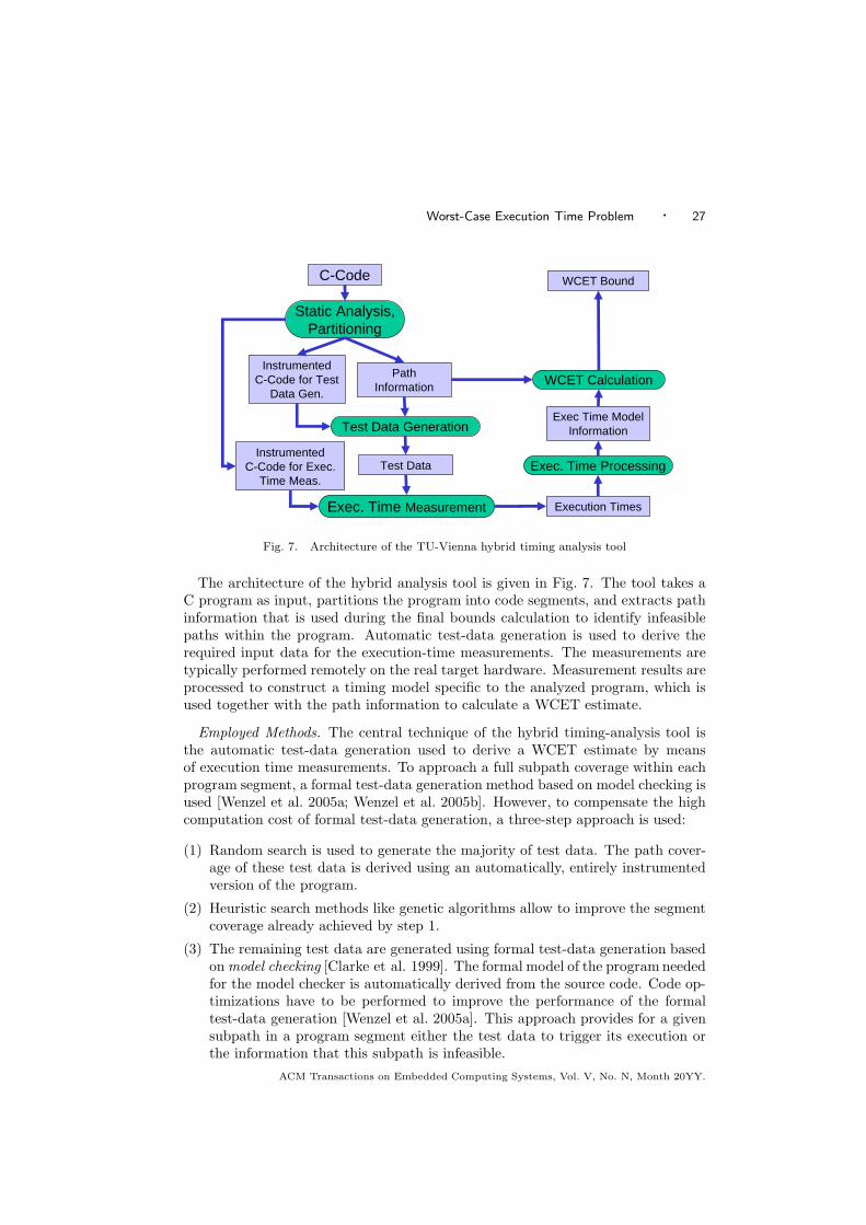
Worst-Case Execution Time Problem · 27

C-Code

Static Analysis,Partitioning

InstrumentedC-Code for Test

Data Gen.

Path Information

Test Data Generation

Test Data

Exec. Time Measurement Execution Times

WCET Calculation

WCET Bound

Exec. Time Processing

Exec Time Model Information

InstrumentedC-Code for Exec.

Time Meas.

Fig. 7. Architecture of the TU-Vienna hybrid timing analysis tool

The architecture of the hybrid analysis tool is given in Fig. 7. The tool takes aC program as input, partitions the program into code segments, and extracts pathinformation that is used during the final bounds calculation to identify infeasiblepaths within the program. Automatic test-data generation is used to derive therequired input data for the execution-time measurements. The measurements aretypically performed remotely on the real target hardware. Measurement results areprocessed to construct a timing model specific to the analyzed program, which isused together with the path information to calculate a WCET estimate.

Employed Methods. The central technique of the hybrid timing-analysis tool isthe automatic test-data generation used to derive a WCET estimate by meansof execution time measurements. To approach a full subpath coverage within eachprogram segment, a formal test-data generation method based on model checking isused [Wenzel et al. 2005a; Wenzel et al. 2005b]. However, to compensate the highcomputation cost of formal test-data generation, a three-step approach is used:

(1) Random search is used to generate the majority of test data. The path cover-age of these test data is derived using an automatically, entirely instrumentedversion of the program.

(2) Heuristic search methods like genetic algorithms allow to improve the segmentcoverage already achieved by step 1.

(3) The remaining test data are generated using formal test-data generation basedon model checking [Clarke et al. 1999]. The formal model of the program neededfor the model checker is automatically derived from the source code. Code op-timizations have to be performed to improve the performance of the formaltest-data generation [Wenzel et al. 2005a]. This approach provides for a givensubpath in a program segment either the test data to trigger its execution orthe information that this subpath is infeasible.

ACM Transactions on Embedded Computing Systems, Vol. V, No. N, Month 20YY.

28 · Reinhard Wilhelm et al.

Based on the measurement results and the path information of the program, theoverall WCET estimate is calculated using integer linear programming.

Limitations of the Tool. As the tool performs static program analysis at thesource code level, it has to be assured that the compiler does not significantlychange the structure of the program code. The hybrid analysis tool guaranteespath coverage for each program segment, therefore every execution scenario is cov-ered by the analysis. However, the tool does not provide state coverage, thus theWCET estimate, though being quite precise, is not guaranteed to be a safe upperbound of the execution times for complex processors having pipelines or caches.Furthermore, the calculation of the tool supports program-flow annotations only atthe granularity of entire program segments.

Supported Hardware Platforms. The targets supported currently include the HCS12,and Pentium processors.

However, as the hybrid approach of the tool does not rely on a model of aprocessor, it is relatively easy to adapt it to other processors. To port the toolto a new processor one has to modify the instrumentation code used to measureexecution times and provide a mechanism to communicate the measurement resultsto the host computer.

6.5 The Chronos Research Prototype from National University of Singapore

Chronos2 is an open-source static WCET analysis tool.

Functionality of the Tool. The purpose of Chronos is to determine a tight upperbound for the execution times of a task running on a modern processor with com-plex micro-architectural features. The input to Chronos is a task written in C andthe configuration of the target processor. The frontend of the tool performs dataflow analysis to compute loop bounds. If it fails to obtain certain loop bounds, userannotations have to be provided. The user may also input infeasible-path informa-tion to improve the accuracy of the results. The frontend maps this informationfrom the source code to the binary executable.

The core of the analyzer works on the binary executable. It disassembles the exe-cutable to generate the control flow graph (CFG) and performs processor-behavioranalysis on this CFG. Chronos supports the analysis of (i) out-of-order pipelines,(ii) various dynamic branch prediction schemes, (iii) instruction caches, and theinteraction among these different features to compute a tight upper bound on theexecution times.

Employed Methods. Chronos employs several innovative techniques to efficientlyobtain safe and tight upper bounds on execution times.

The core of the analyzer determines upper bounds of execution times of eachbasic block under various execution contexts such as correctly predicted or mis-predicted jump of the preceding basic blocks and cache hits/misses within thebasic block [Li 2005]. Determining these bounds is challenging for out-of-orderprocessor pipelines due to the presence of timing anomalies. It requires the costlyenumeration of all possible schedules of instructions within a basic block. Chronos

2Chronos, according to Greek mythology, is the personification of time.

ACM Transactions on Embedded Computing Systems, Vol. V, No. N, Month 20YY.

Worst-Case Execution Time Problem · 29

avoids this enumeration via a fixed-point analysis of the time intervals (insteadof concrete time instances) at which the instructions enter/leave different pipelinestages [Li et al. 2004].

Next, the analyzer employs Integer Linear Programming (ILP) to bound thenumber of executions corresponding to each context. This is achieved by boundingthe number of branch mispredictions and instruction cache misses. Here ILP isused to accurately model branch prediction, instruction cache as well as their inter-action [Li et al. 2005]. The analysis of branch prediction is generic and parameteri-zable w.r.t. the commonly used dynamic branch prediction schemes including GAgand gshare [Mitra et al. 2002]. Instruction caches are analyzed using the ILP-basedtechnique proposed by Li, Malik, and Wolfe [Li et al. 1999]. However, the integra-tion of cache and branch prediction requires analyzing the constructive and destruc-tive timing effects due to cache blocks being “prefetched” along the mispredictedpaths. This complex interaction is accounted for in the analyzer [Li et al. 2003] bysuitably extending the instruction cache analysis.

Finally, bounds calculation is implemented by the IPET technique (see Sec-tion 3.4) by converting the loop bounds and user provided infeasible-path infor-mation to linear flow constraints.

Limitations of the Tool. Chronos currently does not analyze data caches. Sincethe focus is mainly on processor-behavior analysis, the tool performs limited dataflow analysis to compute loop bounds. The tool also requires user feedback forinfeasible program paths.

Supported Hardware Platforms. Chronos supports the processor model of Sim-pleScalar [Austin et al. 2002] sim-outorder simulator, a popular cycle-accuratemicro-architectural simulator. The tool deliberately targets a simulated processormodel so that the processor can be easily configured with different pipeline, branchprediction, and instruction cache options. This allows the user to evaluate theefficiency, scalability, and accuracy of the WCET analyzer for various processorconfigurations without requiring the actual hardware. Moreover, the source codeof the entire tool is publicly available allowing the user to easily extend and adaptit for new architectural features and estimation techniques.

6.6 The Heptane tool of IRISA, Rennes

Heptane is an open-source static WCET analysis tool released under GPL license.

Functionality of the Tool. The purpose of Heptane is to obtain upper boundsfor the execution times of C programs by a static analysis of their code (source codeand binary code). The tool analyses the source and/or binary format dependingon the calculation method the tool is parameterized to work with.

Employed Methods. Heptane embeds in the same analysis tool a timing schema-based and an ILP-based method for bound calculation (see Sections 3.4 and 2.3.5).The former method produces quickly safe, albeit in some circumstances overesti-mated upper bounds for a code snippet, while the latter requires more computingpower, but yields tighter results. The two calculation methods cannot be used si-multaneously on fragments of the same task. The timing-schema method operateson the task’s syntactic structure, which is extracted from the source code. The

ACM Transactions on Embedded Computing Systems, Vol. V, No. N, Month 20YY.

30 · Reinhard Wilhelm et al.

ILP-based method exploits the task’s control-flow graph extracted from the task’sbinary.

Finding the upper bound of a loop requires the knowledge of the maximum num-ber of loop iterations. Heptane requires the user to give this information throughsymbolic annotations in the source program. Annotations are designed to supportnon-rectangular and even non-linear loops (nested loops whose number of iterationsarbitrarily depends on the counter variables of outer loops) [Colin and Puaut 2000].The final bound is computed using an external evaluation tool (Maple and Maximafor the computation method based on timing schemata, lp solve and CPLEX forthe method based on ILP).

Heptane integrates mechanisms to take into account the effect of instructioncaches, pipelines and branch prediction.

—Pipelines are tackled by an off-line simulation of the flow of instructions throughthe pipelines.

—An extension of Frank Mueller’s so-called static cache simulation [Mueller 2000],based on data flow analysis is implemented in the tool. It classifies every instruc-tion according to its worst-case behavior with respect to the instruction cache. In-struction categories take into account loop nesting levels. The Heptane tool takesas input the memory map of the code (cacheable vs. uncacheable code regions,address range of scratchpad memory, if any) as well as the contents of lockedcache regions if a cache locking mechanism is used [Puaut and Decotigny 2002].

—An approach derived from static cache simulation is used to integrate the effect ofbranch predictors based on a cache of recently taken branches [Colin and Puaut 2000].

The modeling of the instruction cache, branch predictor and pipeline produce re-sults expressed in a microarchitecture-independent formalism [Colin and Puaut 2001a],thus allowing Heptane to be easily modified or retargeted to a new architecture.

Limitations of the Tool

—No automatic flow analysis (loop bounds are given manually as annotations at thesource code level), no detection of mutually exclusive or infeasible paths, resultingin pessimistic upper bounds for some tasks (e.g. [Colin and Puaut 2001b]).

—The bound-calculation method based on timing schemata currently does notsupport compiler optimizations that cause a mismatch between the task’s syntax-tree and control flow graph.

—No support for data cache analysis.

—Limited number and types of target processors (currently limited to scalar pro-cessors with in-order execution) and only the gcc compiler.

Supported Hardware Platforms. Heptane is designed to produce timing infor-mation for in-order monoprocessor architectures (Pentium1 - accounting for oneinteger pipeline only, StrongARM 1110, Hitachi H8/300, and MIPS as a virtualprocessor with an overly simplified timing model).

6.7 SWEET (SWEdish Execution Time tool)

SWEET was previously developed in Malardalen University, C-Lab in Paderborn,and Uppsala University. The development has now fully moved to Malardalen

ACM Transactions on Embedded Computing Systems, Vol. V, No. N, Month 20YY.

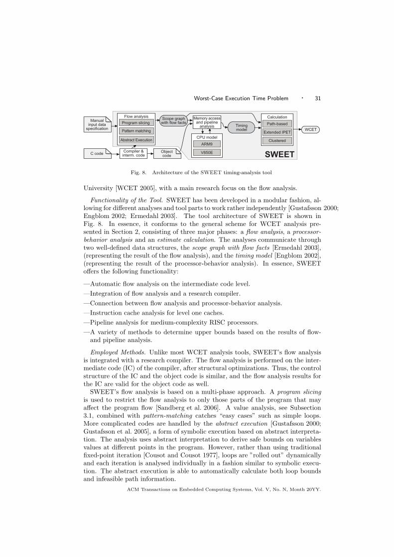
Worst-Case Execution Time Problem · 31

Timingmodel

CPU model

V850E

ARM9

WCET

Calculation

Path-based

Extended IPET

Clustered

SWEETObjectcode

Scope graphwith flow facts

Memory accessand pipeline

analysis

Compiler &interm. code

Manualinput data

specification

C code

Flow analysis

Program slicing

Abstract Execution

Pattern matching

Fig. 8. Architecture of the SWEET timing-analysis tool

University [WCET 2005], with a main research focus on the flow analysis.

Functionality of the Tool. SWEET has been developed in a modular fashion, al-lowing for different analyses and tool parts to work rather independently [Gustafsson 2000;Engblom 2002; Ermedahl 2003]. The tool architecture of SWEET is shown inFig. 8. In essence, it conforms to the general scheme for WCET analysis pre-sented in Section 2, consisting of three major phases: a flow analysis, a processor-behavior analysis and an estimate calculation. The analyses communicate throughtwo well-defined data structures, the scope graph with flow facts [Ermedahl 2003],(representing the result of the flow analysis), and the timing model [Engblom 2002],(representing the result of the processor-behavior analysis). In essence, SWEEToffers the following functionality:

—Automatic flow analysis on the intermediate code level.

—Integration of flow analysis and a research compiler.

—Connection between flow analysis and processor-behavior analysis.

—Instruction cache analysis for level one caches.

—Pipeline analysis for medium-complexity RISC processors.

—A variety of methods to determine upper bounds based on the results of flow-and pipeline analysis.

Employed Methods. Unlike most WCET analysis tools, SWEET’s flow analysisis integrated with a research compiler. The flow analysis is performed on the inter-mediate code (IC) of the compiler, after structural optimizations. Thus, the controlstructure of the IC and the object code is similar, and the flow analysis results forthe IC are valid for the object code as well.

SWEET’s flow analysis is based on a multi-phase approach. A program slicingis used to restrict the flow analysis to only those parts of the program that mayaffect the program flow [Sandberg et al. 2006]. A value analysis, see Subsection3.1, combined with pattern-matching catches “easy cases” such as simple loops.More complicated codes are handled by the abstract execution [Gustafsson 2000;Gustafsson et al. 2005], a form of symbolic execution based on abstract interpreta-tion. The analysis uses abstract interpretation to derive safe bounds on variablesvalues at different points in the program. However, rather than using traditionalfixed-point iteration [Cousot and Cousot 1977], loops are ”rolled out” dynamicallyand each iteration is analysed individually in a fashion similar to symbolic execu-tion. The abstract execution is able to automatically calculate both loop boundsand infeasible path information.

ACM Transactions on Embedded Computing Systems, Vol. V, No. N, Month 20YY.

32 · Reinhard Wilhelm et al.

SWEET’s processor-behavior analysis is highly decoupled from the flow analy-sis, and based on a two-phase approach. In the first phase, the memory accessanalysis, memory areas accessed by different instructions are determined. If thetarget hardware has an instruction cache, an instruction-cache analysis similarto [Ferdinand et al. 1999] is also performed. The result of the analysis is a setof “execution facts” which are used in the pipeline analysis. Such facts specifythe memory area(s) that an instruction may reference or if the instruction may hitand/or miss the cache. Execution facts can also specify other factors like assump-tions on branch prediction outcomes, and the precise set available depends on thetarget processor.

The pipeline analysis is performed by simulating object code sequences through atrace-driven cycle-accurate CPU model. The CPU model needs to be controllable sothat the execution facts can correctly be accounted for in each instruction, and theinstruction trace followed as provided (branch instructions have to follow the trace,for example). The execution facts are used to enforce worst-case timing behaviour ofthe instructions. For data dependent instructions the worst-case timing is assumed,unless execution facts specify otherwise. The pipeline analysis has been explicitlydesigned to allow standard CPU simulators to be used as CPU models. However,this requires that the simulator is clock-cycle accurate, can be forced to perform itssimulation according to given instruction sequences and corresponding executionfacts, and does not suffer from timing anomalies.

Consecutive simulation runs starting with the same basic block in the code arecombined to find timing effects across sequences of two or more blocks in thecode [Engblom 2002]. The analysis assumes that there is a known upper boundon the length of block sequences that can exhibit timing effects; this value can begreater than two even on quite simple processors.

SWEET’s estimate calculation phase support three different type of calculationtechniques, all taking the same two data structures as input. A fast path-based tech-nique [Stappert et al. 2001; Ermedahl 2003; Stappert 2004], a global IPET tech-nique [Ermedahl 2003], and a hybrid clustered technique [Ermedahl et al. 2005;Ermedahl 2003]. The clustered calculation can perform both local IPET and/orlocal path-based calculations (the decision on what to use is based on the flowinformation available for the specific program part under analysis).

SWEET uses DOT from GraphViz [Gansner and North 2000] to graphically vi-sualize its results.

Limitations of the Tool. Each part of the tool, flow analysis, processor-behavioranalysis, and bound calculation have their individual limitations.

The flow analysis can handle ANSI-C programs including pointers, unstructuredcode, and recursion. However, to make use of the automatic flow analysis theprogram must be compiled with the research compiler that SWEET is integratedwith, otherwise flow facts must be manually given. There are also some limitationsinherent to the used research compiler, e.g. the use of dynamically allocated memoryis currently not supported, and annotations will be needed in such cases.

The current memory access analysis does not handle data caches. Only one-levelinstruction caches are supported. The pipelines that are amenable to SWEET’spipeline analysis are limited to in-order pipelines with bounded long-timing effects

ACM Transactions on Embedded Computing Systems, Vol. V, No. N, Month 20YY.

Worst-Case Execution Time Problem · 33

and no timing anomalies. In particular, out-of-order pipelines are not handled.The path-based bound calculation requires that the code of the task is well-

structured. The IPET-based and clustered calculation methods can handle arbi-trary task graphs.

Supported Hardware Platforms. SWEET’s processor-behavior analysis currentlysupports the ARM9 and the NEC V850E. The V850E model has been validatedagainst actual hardware, which the ARM9 has not.

6.8 Research Prototype from Chalmers University of Technology

This tool is a research prototype that was developed to evaluate new concepts forthe determination of execution-time bounds for tasks executed on high-performancemicroprocessors featuring pipelining and multi-level caching techniques.

Functionality of the Tool. The developed tool is capable of automatically derivingsafe upper bounds for tasks’ binaries using a subset of the Power-PC instructionset architecture. It is sometimes possible to derive the exact WCET, in case theworst-case input of the task is known.

Additional functionality:

—Integration of path and timing analysis through symbolic cycle-level execution ofthe task on a detailed architectural simulation model extended to handle unknowninput data values [Lundqvist and Stenstrom 1999b; Lundqvist 2002].

—Binary code transformation techniques that eliminate timing anomalies, whichmay occur when tasks are run on processors where instructions are scheduleddynamically [Lundqvist and Stenstrom 1999c; Lundqvist 2002].

—A data cache analysis method that can identify data structures that can be safelycached - called predictable - so as to improve the worst-case cache performance.Under this method, data structures with unpredictable access patterns are iden-tified and tagged as non-cacheable [Lundqvist and Stenstrom 1999a].

—A method that can determine the worst-case data-cache performance for data ac-cesses to predictable data structures whose exact location in the address space isstatically unknown. This method can be applied to improve worst-case cache per-formance for e.g. procedures whose input parameters are pointers to data struc-tures whose access patterns are predictable, but whose locations in the memoryspace are not known until run-time [Lundqvist 2002].

Employed Methods. Simulation models have been used for some time to es-timate the execution time for tasks on future architectures making use of ad-vanced pipelining and caching techniques. One such example is the SimpleScalartoolset [Austin et al. 2002]. A key advantage of this approach is that it is possibleto derive arbitrarily accurate estimations of the execution time for a task for agiven set of input data and assuming sufficient detail of the timing model of thearchitectural simulator. Unfortunately, as the input data is unknown for a WCETanalyzer, such simulation models cannot be used off-hand.

Concepts have been developed that leverage on the accuracy of architectural tim-ing models to make tight, but still safe estimates of the execution-time bounds.One key concept developed is cycle-level symbolic program simulation. First,

ACM Transactions on Embedded Computing Systems, Vol. V, No. N, Month 20YY.

34 · Reinhard Wilhelm et al.

loop bounds, branch conditions etc., which are not input-data dependent willbe calculated as the task is executed symbolically on the architectural simula-tor. However, in order to handle unknown input data, the instruction-set sim-ulator was extended with the capability of handling unknown parts of execu-tion states. For example, if a branch condition depends on unknown input data,both paths are executed. Inevitably, this may result in the well-known path ex-plosion problem in program loops with a large number of iterations. A path-merging approach excludes the paths that may not be part of the worst-caseexecution path through the task. The analysis that determines which paths toexclude must take into account what timing effect they may have in the future.This involves analysis of worst-case performance taking microarchitectural fea-tures such as pipelining and caching into account. Methods have been devel-oped and integrated to do this analysis for a range of architectural features in-cluding multi-level instruction and data caches [Lundqvist and Stenstrom 1999b;Lundqvist and Stenstrom 1999a] and multiple-issue pipelines with dynamic instruc-tion scheduling [Lundqvist and Stenstrom 1999c]. How often path merging is car-ried out is a tradeoff between computational speed and accuracy of the analysis andis investigated in [Lundqvist 2002]. The described symbolic execution of tasks hasbeen shown to exclude some infeasible paths thereby making the execution-timebounds tighter.

Limitations of the Tool. The user has to provide annotations for loops with un-known termination properties.

An inherent limitation of the approach is the computational complexity of theanalysis. While the path-merging method partly addresses this concern, it alsointroduces over-estimation of the WCET. Therefore, we believe that this approachis most relevant in the final stage of the development cycle, when the design spacehas been narrowed down so that one can afford the long-running simulations forlimited aspects of the entire system.

Supported Hardware Platforms. Our tool currently supports a fairly rich subsetof the PowerPC instruction set architecture. We have also integrated architecturaltiming models for some implementations of the PowerPC featuring dual-instructionissue, a dynamically scheduled pipeline, a parameterized cache hierarchy with splitfirst-level set-associative instruction and data caches and a unified second-levelcache. The cache and block size as well as the associativity of each cache is param-eterized.

6.9 SymTA/P Tool of TU Braunschweig, Germany

Functionality of the Tool. The purpose of SymTA/P is to obtain upper and lowerexecution time bounds of C programs running on microcontrollers. SymTA/P is anacronym of SYMbolic Timing Analysis for Processes. The key idea of SymTA/P isto combine platform independent path analysis on source code level and platformdependent measurement methodology on object code level, using an actual targetsystem. The main benefit is that this hybrid analysis can easily be re-targeted toa new hardware platform.

The execution time measurement can be obtained by an off-the-shelf cycle-accurate processor simulator or by an evaluation board. Instruction cache as well as

ACM Transactions on Embedded Computing Systems, Vol. V, No. N, Month 20YY.

Worst-Case Execution Time Problem · 35

data cache behavior is analyzed for a single uninterrupted task execution. Further-more, the cache related preemption delay for fixed priority preemptive real-timesystems for direct mapped and associative caches is analyzed and integrated in acache-aware response time analysis. To be efficient, cache analysis requires that atask execution trace can be generated that is uninterrupted by cache misses, eitherbecause the task is small enough to fit in the cache or because the evaluation systemoffers sufficient on-chip fast memory, e.g. scratchpad RAM. If that is not available,then an appropriate simulator must be used instead.

Employed Methods. The hybrid approach consists of a static program path anal-ysis and a measurement for the execution time of program segments. In most staticanalyses of execution times, a basic block has been assumed as the smallest entity.However often a program consists of a single feasible execution path (SFP) only.Such a SFP is a sequence of basic blocks where the execution sequence is invariantto input data [Wolf 2002; Wolf et al. 2001; Ye and Ernst 1997].

SymTA/P uses symbolic analysis on the abstract syntax tree to identify suchsingle feasible paths (SFP) at the source code level. The result is a control-flowgraph with nodes containing single feasible paths or basic blocks that are partof a multiple feasible path. A single feasible path can reach beyond basic blockboundaries, for example, a fast Fourier transformation or a FIR filter. In thesecases, the program contains loops with several if-then-else statements which areinput independent. This means that the branch direction depends only on localvariables with known values, for example the loop iteration count. Therefore theentire loop represents an SFP and is represented by a single node. The main benefitof SFPs is a smaller number of instrumentation points.

In a second step, the execution time for each node is estimated. Off-the-shelfprocessor simulators or standard cost-efficient evaluation boards can be used. The Csource code is instrumented with measurement points that mark the beginning andthe end of each node. Such a measurement point is linked to a platform dependentmeasurement procedure, such as accessing the system clock or internal timer. For aprocessor simulator the instrumentation can use a processor debugger command tostop the simulation and store the internal system clock. Then, the entire C-programwith measurement points is compiled, linked and executed on the evaluation board(or simulated on the processor simulator). During this measurement, a safe initialstate cannot be assured in all cases. Therefore an additional time delay is addedthat covers a potential underestimation during such a measurement.

At this step, SymTA/P assumes that each memory access takes constant time.For timing analysis, input data for a complete branch coverage must be supplied.A complete branch coverage means, that with a given set of input data all branchesand other C statements are at least executed once. This criterion requires the userto specify a considerably fewer number of input data than a full path coveragebecause combinations of execution paths need not be considered. This advantagecomes with the drawback that it adds a conservative overhead to cover pipeliningeffects between nodes.

The constant memory access time assumption is revised by analyzing the instruction-cache and the data-cache behavior [Wolf et al. 2002]. When using a processor sim-ulator, the memory access trace for each node is generated using a similar method-

ACM Transactions on Embedded Computing Systems, Vol. V, No. N, Month 20YY.

36 · Reinhard Wilhelm et al.

ology as the execution time measurements. The traced memory accesses are an-notated to the corresponding node in the control flow graph. A data flow analysistechnique is used to propagate the information which cache lines are available ateach node. Pipelining effects between nodes are not directly modeled, instead a con-servative overhead corresponding to starting with an empty pipeline is assumed.

The longest and shortest path in the control flow graph are found by IPET (seeSection 3.4) and Fig. 5. The time for each node is given by the measured executiontime and the statically analyzed cache access behavior. This framework has alsobeen used to calculate the power consumption of a program [Wolf et al. 2002]. Loopbounds have to be specified by the user, if the loop condition is input dependent.

If preemptive scheduling is used, cache blocks might be replaced by higher pri-ority tasks. SymTA/P considers the cache behavior of the preempted and pre-empting task to compute the maximum cache related preemption delay. This de-lay is considered in cache-aware response time analysis [Staschulat and Ernst 2004][Staschulat et al. 2005].

SymTA/P uses a static analysis approach for data cache behavior, which com-bines symbolic execution to identify input dependent memory accesses and usesinteger linear programming to bound the worst case data cache behavior for inputdependent memory accesses [Staschulat and Ernst 2006].

Limitations of the Tool. The measurement on an evaluation board is more accu-rate if the program paths between measurements points are longer. If many basicblocks are measured individually the added time delays to cover pipelining effectswould lead to an overestimation of the total worst case execution time. Data-dependent execution times of single instructions are not explicitly considered. It isassumed that input data covers the worst case regarding data-dependent instructionexecution time. Input data has to be provided that generates complete branch cov-erage. Such patterns are usually available from functional test. The precision of thefinal analysis depends on the measurement environment. Especially for evaluationboards the interference of the measurement instrumentation has to be a constantfactor to obtain sufficiently accurate results. Currently, the approach assumes asequential memory access behavior where the CPU stalls during a memory access.

Supported hardware platforms. C programs on the following micro-controllershave been analyzed: ARM architectures (e.g. ARM9), TriCore, StrongARM, C167,and i8051. The software power analysis has been applied to SPARClite. Further-more, an open interface for processor simulators and a measurement framework forevaluation boards is provided.

6.10 The RapiTime tool of Rapita Systems Ltd., York, UK

RapiTime aims at medium to large real-time embedded systems on advanced pro-cessors. The RapiTime tool targets the automotive electronics, avionics and telecom-munications industries.

Functionality of the Tool. Rapitime is a measurement-based tool, i.e., it derivestiming information of how long a particular section of code (generally a basic block)takes to run from measurements. Measurement results are combined according tothe structure of the program to determine an estimate for the longest path through

ACM Transactions on Embedded Computing Systems, Vol. V, No. N, Month 20YY.

Worst-Case Execution Time Problem · 37

the program,

RapiTime not only computes an estimate for the WCET of a program as a single(integer) value, but also the whole probability distribution of the execution timeof the longest path in the program (and other subunits). This distribution hasa bounded domain (an absolute upper bound, the WCET estimate, and a lowerbound).

The input of RapiTime is either a set of source files (C or Ada) or an executable.The user also has to provide test data from which measurements will be taken. Theoutput is a browsable HTML report with description of the WCET prediction andactual measured execution times, split for each function and subfunction.

Timing information is captured on the running system by either a software instru-mentation library, a lightweight software instrumentation with external hardwaresupport, purely non-intrusive tracing mechanisms (like Nexus and ETM) or eventraces from CPU simulators.

The user can add annotations in the code to guide how the instrumentation andanalysis process will be performed, to bound the number of iterations of loops, etc.

The RapiTime tool supports various architectures, adapting the tool for newarchitectures requires porting the object code reader (if needed) and determininga tracing mechanism for that system.

RapiTime is the commercial quality version of the pWCET tool developed at theReal-Time Systems Research Group at the University of York.

Employed Methods. The RapiTime tool is structure-based and works on a treerepresentation of the program. The structure is derived from either the source codeor from the direct analysis of executables.

The timing of individual blocks is derived from extensive measurements extractedfrom the real system. RapiTime not only computes the maximum of the measuredtimes but whole probability distributions [Bernat et al. 2002; Bernat et al. 2005].The WCET estimates are computed using an algebra of probability distributions.

The timing analysis of the program can be performed on different contexts, there-fore allowing to analyze, for instance, each different call to a function individually.The level of detail and how many contexts are analyzed is controlled by annota-tions. RapiTime also allows to analyze different loop iterations by virtually un-rolling loops. For each of these loop contexts, loop bounds are derived from actualmeasurements (or annotations).

Limitations of the Tool. The RapiTime tool does not rely on a model of theprocessor, so in principle it can model any processing unit (even with out-of-orderexecution, multiple execution units, various hierarchies of caches etc). The lim-itation is put on the need to extract execution traces which require some codeinstrumentation and a mechanism to extract these traces from the target system.Regarding source code level, RapiTime cannot analyze programs with recursionand with non-statically analyzable function pointers.

Supported Hardware Platforms. Motorola processors (including MPC555, HCS12,etc), ARM, MIPS, NecV850.

ACM Transactions on Embedded Computing Systems, Vol. V, No. N, Month 20YY.

38 · Reinhard Wilhelm et al.

7. EXPERIENCE

Three commercial WCET tools are available, aiT, Bound-T, and RapiTime. Thereare extensive reports about industrial use [Thesing et al. 2003; Sandell et al. 2004;Souyris et al. 2005; Byhlin et al. 2005; Holsti et al. 2000b; Holsti et al. 2000a]. Infact, tools are under routine use in the aeronautics and the automotive industries.They enjoy very positive feedback concerning speed, precision of the results, andusability. The aeronautics industry uses them in the development of the most safety-critical systems, e.g. the fly-by-wire systems for the Airbus A380. The used WCETtool will be qualified as verification tool in the sense of the international avionicsstandard for safety-critical software, RTCA/DO-178B (Software Considerations inAirborne Systems and Equipment Certification Requirements) for Level A Code.

There are not many published benchmark results about timing-analysis tools.[Lim et al. 1995] is a study done by the authors of a method carefully explainingthe reasons for over-estimation. [Thesing et al. 2003; Souyris et al. 2005] reportexperiences made by developers. The developers are experienced, and the tool isintegrated into the development process. We summarize these three comparablebenchmarks in Table I. They seem to exhibit a surprising paradox, benchmarkspublished earlier offer better results regarding the degree of overestimation, al-though significant methodological progress has been made in the meantime. Thereason lies in the fact that the advancement of processor architectures and in partic-ular the divergence of processor and memory speeds have made the challenge of tim-ing analysis harder. Both have increased the timing variability and thus the penaltyfor the lack of knowledge in analysis results. Let’s take the cache-miss penalty asan example, the single cause with highest weight. In [Lim et al. 1995], publishedin 1995, a cache-miss penalty of 4 cycles was assumed. In [Thesing et al. 2003],a cache-miss penalty of roughly 25 was given, and finally in the setting describedin [Souyris et al. 2005], the cache-miss penalty was between 60 internal cycles for aworst-case access to an instruction in SDRAM and roughly 200 internal cycles foran access to data over the PCI bus. Thus, any overestimation should be consid-ered in the context of the given architecture. An overestimation of 30% in 2005 asreported in [Souyris et al. 2005] means a huge progress compared to an overestima-tion of 30% reported in 1995 [Lim et al. 1995]! On the other hand, static methodsare capable of predicting exact WCETs on simple microcontrollers without caches,deep pipelines, and speculation.

The Malardalen University WCET-research group has performed several indus-trial WCET case-studies as M.Sc. Thesis projects using the SWEET [Carlsson et al. 2002]and aiT [Sandell et al. 2004; Byhlin et al. 2005; Eriksson 2005; Zhang 2005; Sehlberg 2005]tools. The students were experts neither on the used timing-analysis tool nor onthe analyzed system. However, they were assisted both by WCET analysis expertsfrom academia and industrial personel with detailed system knowledge.

The case-studies show that it is possible to apply static WCET analysis to avariety of industrial systems and codes. The tools used performed well and derivedsafe upper timing bounds. However, detailed knowledge of the analyzed code andmany manual annotations were often required to achieve reasonably tight bounds.These annotations were necessary to give the analysis enough knowledge aboutprogram flow constraints and in some cases constraints on addresses of memory

ACM Transactions on Embedded Computing Systems, Vol. V, No. N, Month 20YY.

Worst-Case Execution Time Problem · 39

Reference Year Cache-miss penalty Overestim.

[Lim et al. 1995] 1995 4 20-30%

[Thesing et al. 2003] 2002 25 15%

[Souyris et al. 2005] 200560 for accessing instructions in SDRAM200 for access over PCI bus

30-50%

Table I. Cache-miss penalties and degrees of overestimation.

accesses. A higher degree of automation and support from the tools, e.g. automaticloop bounds calculation, would in most cases have been desirable.

The case-studies also show that single timing bounds, covering all possible sce-narios, are not always what you want. For several analyzed systems it was moreinteresting to have different WCET bounds for different running modes or systemconfigurations rather than a single WCET bound. The latter would in most caseshave been a gross overapproximation. In some cases, it was also possible to manu-ally derive a parametrical formula [Sandell et al. 2004; Byhlin et al. 2005], showinghow the WCET estimate depends on some specific system parameters.

The case-studies were done for processors without cache. The overestimationswere mostly in the range 5-15% as compared with measured times. Measurementswere in some cases done with emulators, and in some cases directly on the hardwareusing oscilloscopes and logical analyzers.

Performance and Size. Table IV in Section 9 lists the maximal size of tasks an-alyzed by the different tools. They vary between 10kByte and 80 kByte of code.Analysis times vary widely depending on the complexity of the processor and itsperiphery and the structure and other characteristics of the software. Analysisof a task for a simple microprocessor such as the C166/ST10 may finish in a fewminutes. Analysis of a complex software, an abstract machine and the code inter-preted by it, and a complex processor has been shown to take in the order of a day,see [Souyris et al. 2005].

Also of interest is the size of the abstract processor models underlying some staticanalysis approaches. They range from 3000 to 11000 lines of C code. This C codeis the result of a translation from a formal model.

8. LIMITATIONS OF THE TOOLS

Determining safe and precise bounds on execution times is a very difficult prob-lem, undecidable in general as is known, but still very complex for programs withbounded iteration and recursion. There are several features whose use will easilyruin precision. Among these are pointers to data and to functions that cannotstatically be resolved, and the use of dynamically allocated data. Most tools willexpect that function calling conventions are observed. Some tools forbid recursion.Currently, only mono-processor targets are supported. Most tools only consideruninterrupted execution of tasks.

9. TOOL COMPARISON

This section shows in a condensed form the most relevant information about thedifferent tools. The following abbreviations for the Vienna tools are used, Vienna M.for Vienna Measurement, Vienna S. for Vienna Static, and Vienna H. for Vienna

ACM Transactions on Embedded Computing Systems, Vol. V, No. N, Month 20YY.

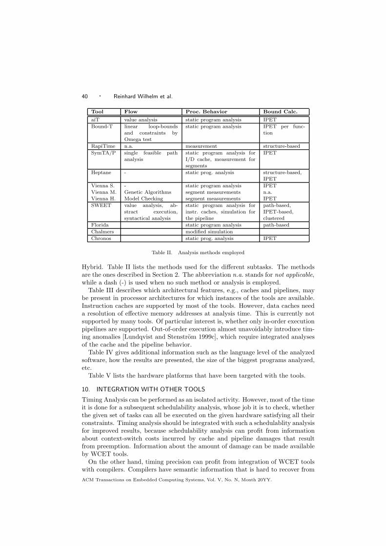
40 · Reinhard Wilhelm et al.

Tool Flow Proc. Behavior Bound Calc.

aiT value analysis static program analysis IPET

Bound-T linear loop-boundsand constraints byOmega test

static program analysis IPET per func-tion

RapiTime n.a. measurement structure-based

SymTA/P single feasible pathanalysis

static program analysis forI/D cache, measurement forsegments

IPET

Heptane - static prog. analysis structure-based,IPET

Vienna S. - static program analysis IPETVienna M. Genetic Algorithms segment measurements n.a.Vienna H. Model Checking segment measurements IPET

SWEET value analysis, ab-stract execution,syntactical analysis

static program analysis forinstr. caches, simulation forthe pipeline

path-based,IPET-based,clustered

Florida static program analysis path-based

Chalmers modified simulation

Chronos static prog. analysis IPET

Table II. Analysis methods employed

Hybrid. Table II lists the methods used for the different subtasks. The methodsare the ones described in Section 2. The abbreviation n.a. stands for not applicable,while a dash (-) is used when no such method or analysis is employed.

Table III describes which architectural features, e.g., caches and pipelines, maybe present in processor architectures for which instances of the tools are available.Instruction caches are supported by most of the tools. However, data caches needa resolution of effective memory addresses at analysis time. This is currently notsupported by many tools. Of particular interest is, whether only in-order executionpipelines are supported. Out-of-order execution almost unavoidably introduce tim-ing anomalies [Lundqvist and Stenstrom 1999c], which require integrated analysesof the cache and the pipeline behavior.

Table IV gives additional information such as the language level of the analyzedsoftware, how the results are presented, the size of the biggest programs analyzed,etc.

Table V lists the hardware platforms that have been targeted with the tools.

10. INTEGRATION WITH OTHER TOOLS

Timing Analysis can be performed as an isolated activity. However, most of the timeit is done for a subsequent schedulability analysis, whose job it is to check, whetherthe given set of tasks can all be executed on the given hardware satisfying all theirconstraints. Timing analysis should be integrated with such a schedulablity analysisfor improved results, because schedulability analysis can profit from informationabout context-switch costs incurred by cache and pipeline damages that resultfrom preemption. Information about the amount of damage can be made availableby WCET tools.

On the other hand, timing precision can profit from integration of WCET toolswith compilers. Compilers have semantic information that is hard to recover from

ACM Transactions on Embedded Computing Systems, Vol. V, No. N, Month 20YY.

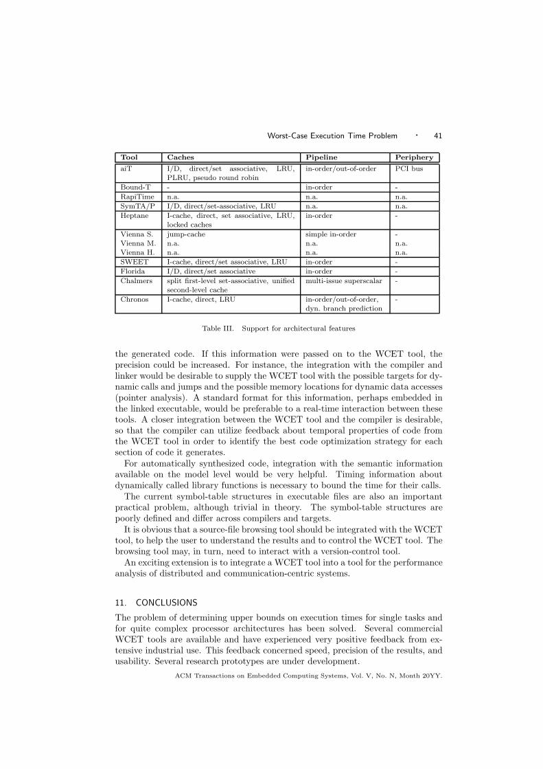
Worst-Case Execution Time Problem · 41

Tool Caches Pipeline Periphery

aiT I/D, direct/set associative, LRU,PLRU, pseudo round robin

in-order/out-of-order PCI bus

Bound-T - in-order -

RapiTime n.a. n.a. n.a.

SymTA/P I/D, direct/set-associative, LRU n.a. n.a.

Heptane I-cache, direct, set associative, LRU,locked caches

in-order -

Vienna S. jump-cache simple in-order -Vienna M. n.a. n.a. n.a.Vienna H. n.a. n.a. n.a.

SWEET I-cache, direct/set associative, LRU in-order -

Florida I/D, direct/set associative in-order -

Chalmers split first-level set-associative, unifiedsecond-level cache

multi-issue superscalar -

Chronos I-cache, direct, LRU in-order/out-of-order,dyn. branch prediction

-

Table III. Support for architectural features

the generated code. If this information were passed on to the WCET tool, theprecision could be increased. For instance, the integration with the compiler andlinker would be desirable to supply the WCET tool with the possible targets for dy-namic calls and jumps and the possible memory locations for dynamic data accesses(pointer analysis). A standard format for this information, perhaps embedded inthe linked executable, would be preferable to a real-time interaction between thesetools. A closer integration between the WCET tool and the compiler is desirable,so that the compiler can utilize feedback about temporal properties of code fromthe WCET tool in order to identify the best code optimization strategy for eachsection of code it generates.

For automatically synthesized code, integration with the semantic informationavailable on the model level would be very helpful. Timing information aboutdynamically called library functions is necessary to bound the time for their calls.

The current symbol-table structures in executable files are also an importantpractical problem, although trivial in theory. The symbol-table structures arepoorly defined and differ across compilers and targets.

It is obvious that a source-file browsing tool should be integrated with the WCETtool, to help the user to understand the results and to control the WCET tool. Thebrowsing tool may, in turn, need to interact with a version-control tool.

An exciting extension is to integrate a WCET tool into a tool for the performanceanalysis of distributed and communication-centric systems.

11. CONCLUSIONS

The problem of determining upper bounds on execution times for single tasks andfor quite complex processor architectures has been solved. Several commercialWCET tools are available and have experienced very positive feedback from ex-tensive industrial use. This feedback concerned speed, precision of the results, andusability. Several research prototypes are under development.

ACM Transactions on Embedded Computing Systems, Vol. V, No. N, Month 20YY.

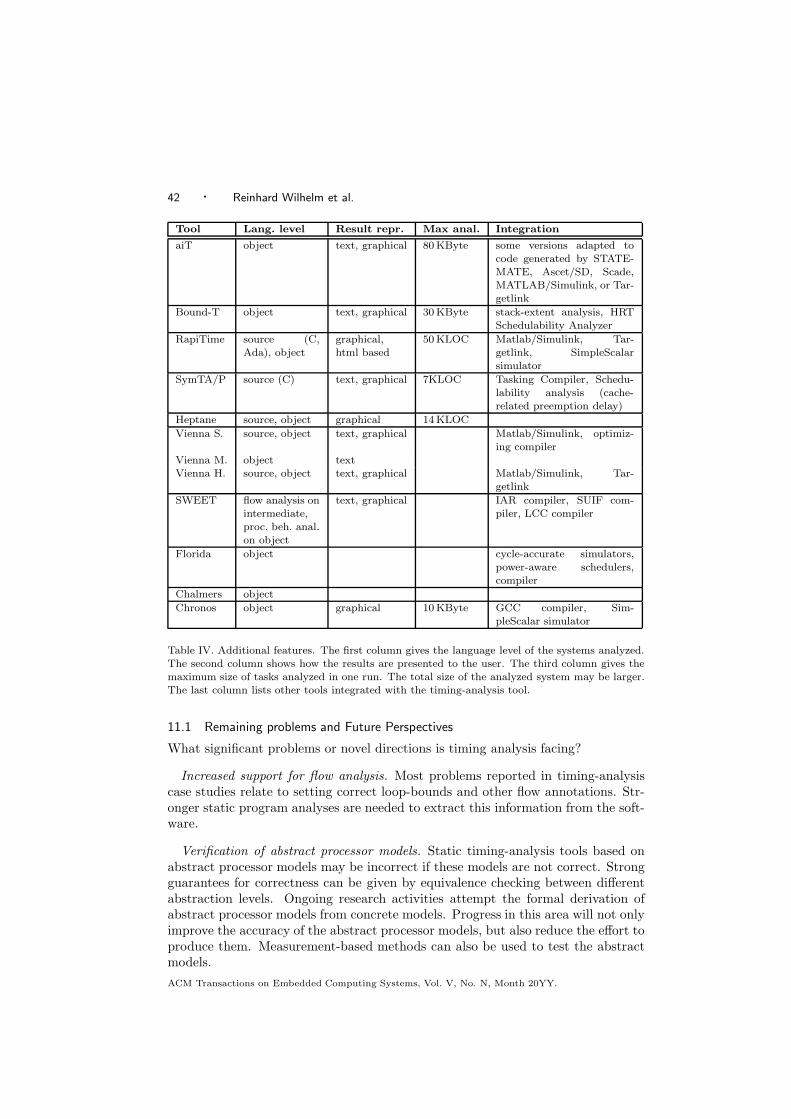
42 · Reinhard Wilhelm et al.

Tool Lang. level Result repr. Max anal. Integration

aiT object text, graphical 80 KByte some versions adapted tocode generated by STATE-MATE, Ascet/SD, Scade,MATLAB/Simulink, or Tar-getlink

Bound-T object text, graphical 30 KByte stack-extent analysis, HRTSchedulability Analyzer

RapiTime source (C,Ada), object

graphical,html based

50 KLOC Matlab/Simulink, Tar-getlink, SimpleScalarsimulator

SymTA/P source (C) text, graphical 7KLOC Tasking Compiler, Schedu-lability analysis (cache-related preemption delay)

Heptane source, object graphical 14 KLOC

Vienna S. source, object text, graphical Matlab/Simulink, optimiz-ing compiler

Vienna M. object textVienna H. source, object text, graphical Matlab/Simulink, Tar-

getlink

SWEET flow analysis onintermediate,proc. beh. anal.on object

text, graphical IAR compiler, SUIF com-piler, LCC compiler

Florida object cycle-accurate simulators,power-aware schedulers,compiler

Chalmers object

Chronos object graphical 10 KByte GCC compiler, Sim-pleScalar simulator

Table IV. Additional features. The first column gives the language level of the systems analyzed.The second column shows how the results are presented to the user. The third column gives themaximum size of tasks analyzed in one run. The total size of the analyzed system may be larger.The last column lists other tools integrated with the timing-analysis tool.

11.1 Remaining problems and Future Perspectives

What significant problems or novel directions is timing analysis facing?

Increased support for flow analysis. Most problems reported in timing-analysiscase studies relate to setting correct loop-bounds and other flow annotations. Str-onger static program analyses are needed to extract this information from the soft-ware.

Verification of abstract processor models. Static timing-analysis tools based onabstract processor models may be incorrect if these models are not correct. Strongguarantees for correctness can be given by equivalence checking between differentabstraction levels. Ongoing research activities attempt the formal derivation ofabstract processor models from concrete models. Progress in this area will not onlyimprove the accuracy of the abstract processor models, but also reduce the effort toproduce them. Measurement-based methods can also be used to test the abstractmodels.

ACM Transactions on Embedded Computing Systems, Vol. V, No. N, Month 20YY.

Worst-Case Execution Time Problem · 43

Tool Hardware platform

aiT Motorola PowerPC MPC 555, 565, and 755, Motorola ColdFire MCF 5307, ARM7TDMI, HCS12/STAR12, TMS320C33, C166/ST10, Renesas M32C/85, InfineonTriCore 1.3

Bound-T Intel-8051, ADSP-21020, ATMEL ERC32, Renesas H8/300, ATMEL AVR, AT-mega, ARM7

RapiTime Motorola PowerPC family, HCS12 family, ARM, NecV850, MIPS3000

SymTA/P various ARM (RealView Suite), TriCore, i8051, C167

Heptane Pentium1, StrongARM 1110, Hitachi H8/300

Vienna S. M68000, M68360, C167Vienna M. C167, PowerPCVienna H. HCS12, Pentium

SWEET ARM9 core, NEC V850E

Florida MicroSPARC I, Intel Pentium, StarCore SC100, Atmel Atmega, PISA/MIPS

Chalmers PowerPC

Chronos SimpleScalar out-of-order processor model with MIPS-like instruction-set-architecture (PISA)

Table V. Supported hardware platforms

Integration of timing analysis with compilation. An integration of static timinganalysis with a compiler can provide valuable information available in the compilerto the timing analysis and thereby improve the precision of analysis results.

Integration with scheduling. Preemption of tasks causes large context-switch costson processors with caches; the preempting task may ruin the cache contents, suchthat the preempted task encounters considerable cache-reload costs when resumingexecution. These context-switch costs may be even different for different combina-tions of preempted and preempting task. These large and varying context-switchcosts violate assumptions underlying many real-time scheduling methods. A newscheduling approach considering the combination of timing analysis and preemp-tive scheduling will have to be developed. SymTA/P provides an integration ofWCET calculation and cache-related preemption delay for schedulability analy-sis [Staschulat et al. 2005].

Interaction with energy awareness. This may concern the trade off between speedand energy consumption. [Jayaseelan et al. 2006] presents a static analysis tech-nique to estimate the worst-case energy consumption of a task on complex micro-architectures. Estimating a bound on energy is non-trivial as it is unsafe to assumeany direct correlation with the bound on execution time. On the other hand, infor-mation computed for WCET determination, e.g., cache behavior, is of high valuefor the determination of energy consumption [Seth et al. 2003].

Design of systems with time-predictable behavior. This is a particularly well-motivated research direction, because several trends in system design make systemsless and less predictable [Thiele and Wilhelm 2004].

There are first proposals in this area. [Anantaraman et al. 2003] propose a vir-tual simple architecture (VISA). A VISA is the pipeline timing specification of ahypothetical simple processor. Upper bounds for execution times are derived fora task assuming the VISA. At run-time, the task is executed speculatively on anunsafe complex processor, and its progress is continuously gauged. If continued

ACM Transactions on Embedded Computing Systems, Vol. V, No. N, Month 20YY.

44 · Reinhard Wilhelm et al.

Tool Contact person Contact information

aiT Christian Ferdinand Email: info@AbsInt.comAbsInt Angewandte Informatik GmbH Phone: +49 681 383 60 0Science Park 1 Fax: +49 681 383 60 20D-66123 Saarbrucken Web: www.AbsInt.comGermany

Bound-T Niklas Holsti Email : info@tidorum.fiTidorum Ltd Phone: +358 (0) 40 563 9186Tiirasaarentie 32 Web: www.tidorum.fiFI-00200 Helsinki Web: www.bound-t.comFinland

RapiTime Guillem Bernat Email: enquiries@rapitasystems.comRapita Systems Ltd. Phone: +44 1904 567747IT Center, York Science Park Fax: +44 1904 567719Heslington Web: www.rapitasystems.comYork YO10 5DGUnited Kingdom

SymTA/P Rolf Ernst, Jan Staschulat Email: ernst|staschulat@ida.ing.tu-bs.deInstitute for Computer and Phone: +49 531 391 3730Communication Network Engineering Fax: +49 531 391 3750Technical University Braunschweig Web: www.ida.ing.tu-bs.de/research/projects/symtaHans-Sommer-Str. 66D-38106 Braunschweig, Germany

Heptane Isabelle Puaut Email: puaut@irisa.frIRISA, ACES Research Group Phone: +33 02 99 84 73 10Campus univ. de Beaulieu Fax: +33 02 99 84 25 2935042 Rennes Cedex, France Web: www.irisa.fr/aces/work/heptane-

demo/heptane.htm l

Vienna Peter Puschner Email: peter.puschner@tuwien.ac.atInst. fur Technische Informatik Phone: 01 58 801 18 227TU Wien Fax: 01 58 69 149A-1040 Wien, Austria

SWEET Bjorn Lisper Email: bjorn.lisper@mdh.seMalardalen University Email: andreas.ermedahl@mdh.seP.O. Box 883 SE-721 23 Email: jan.gustafsson@mdh.seSE 72123 Vasteras Phone: +46 21 151 709Sweden Web: www.mrtc.mdh.se/projects/wcet/

Florida David Whalley Email: whalley@cs.fsu.eduFlorida State UniversityFrank Mueller Email: mueller@cs.ncsu.eduNorth Carolina State UniversityChris Healy Email: chris.healy@furman.eduFurman University, USA

Chalmers Per Stenstrom Email: pers@ce.chalmers.seDepartment of Computer Engineering Phone: +46 31 772 1761Chalmers University of Technology Fax: +46 31 772 3663

S-412 96 Goteborg, Sweden

Chronos Tulika Mitra, Email: tulika@comp.nus.edu.sg,Abhik Roychoudhury, Email: abhik@comp.nus.edu.sgXianfeng Li, Email: lixianfe@comp.nus.edu.sgNational University of Singapore www.comp.nus.edu.sg/˜rpembed/chronos

Table VI. Contact information for the tools.

ACM Transactions on Embedded Computing Systems, Vol. V, No. N, Month 20YY.

Worst-Case Execution Time Problem · 45

safe progress appears to be in jeopardy, the complex processor is reconfigured toa simple mode of operation that directly implements the VISA, thereby explicitlybounding the task’s overall execution time. Progress is monitored at intra-taskcheckpoints, which are derived from upper bounds and unsafe predictions of execu-tion times for subtasks [Anantaraman et al. 2004]. Hence, VISA shifts the burdenof bounding the execution times of tasks, in part, to hardware by supporting twoexecution modes within a single processor. [Puschner 2005] proposes to transformsets of program paths to single paths by predicate conversion as in code generationfor processors with predicated execution. The disadvantage is the loss in perfor-mance resulting from the need to execute predicated paths that would originallynot be executed.

Any proposal increasing predictability plainly at the cost of performance willmost likely not be accepted by developers.

Extension to component-based design. Timing-Analysis methods should be madeapplicable to component-based design and systems built on top of real-time oper-ating systems and using real-time middleware.

11.2 Architectural Trends

The hardware used in creating an embedded real-time system has a great effect onthe ease of predictability of the execution time of programs.

The simplest case are traditional 8-bit and 16-bit processors with simple archi-tectures. In such processors, each instruction basically has a fixed execution time.Such processors are easy to model from the hardware timing perspective, and theonly significant problem in WCET analysis is how to determine the program flow.

There is also a class of processors with simple in-order pipelines, which are foundin cost-sensitive applications requiring higher performance than that offered byclassic 8-bit and 16-bit processors. Examples are the ARM7 and the recent ARMCortex R series. Over time, these chips can be expected to replace the 8-bit and16-bit processors for most applications. With their typically simple pipelines andcache structures, relatively simple and fast WCET hardware analysis methods canbe applied.

At the high-end of the embedded real-time spectrum, performance requirementsfor applications like flight control and engine control force real-time systems design-ers to use complex processors with caches and out-of-order execution. Examplesare the PowerPC 750, PowerPC 7448, and ARM11 families of processors. Analyz-ing such processors requires more advanced tools and methods, especially in thehardware analysis.

The mainstream of computer architecture is steadily adding complexity and spec-ulative features in order to push the performance envelope. Architectures such asthe AMD Opteron, Intel Pentium 4 and Pentium-M, and IBM Power5 use multiplethreads per processor core, deep pipelines, and several levels of caches to achievemaximum performance on sequential programs.

This mainstream trend of ever-more complex processors is no longer as dominantas it used to be, however. In recent years, several other design alternatives haveemerged in the mainstream, where the complexity of individual processor cores hasbeen reduced significantly.

ACM Transactions on Embedded Computing Systems, Vol. V, No. N, Month 20YY.

46 · Reinhard Wilhelm et al.

Many new processors are designed by using several simple cores instead of asingle or a few complex cores. This design gains throughput per chip by runningmore tasks in parallel, at the expense of single-task performance. Examples arethe Sun Niagara chip which combines 8 in-order four-way multithreaded cores on asingle chip [Olukotun and Hammond 2005], and the IBM-designed PowerPC for theXbox 360, using three two-way multithreaded in-order cores [Krewell 2005]. Thesedesigns are cache-coherent multiprocessors on a chip, and thus have a fairly complexcache- and memory system. The complexity of analysis moves from the behaviorof the individual cores to the interplay between them as they access memory.

Another very relevant design alternative is to use several simple processors withprivate memories (instead of shared memory). This design is common in mobilephones, where you typically find an ARM main processor combined with one ormore DSPs on a single chip. Outside the mobile phone industry, the IBM-Sony-Toshiba Cell processor is a high-profile design using a simple in-order PowerPC corealong with eight synergistic processing elements (SPEs) [Hofstee 2005]. The Cellwill make its first appearance in the Sony PlayStation 3 gaming console, but IBMand Mercury Computing systems are pushing the Cell as a general-purpose real-time processor for high-performance real-time systems. The SPEs in the Cell aredesigned for predictable performance, and use local program-controlled memoriesrather than caches, just like most DSPs. Thus, this type of architecture providesseveral easy-to-predict processors on a chip as an alternative to a single hard-to-predict processor.

Field-programmable gate arrays (FPGAs) are another design alternative for someembedded applications. Several processor architectures are available as “soft cores”that can be implemented in an FPGA together with application-specific logic andinterfaces. Such processor implementations may have application-specific timingbehavior which may be challenging for off-the-shelf timing analysis tools, but theyare also likely to be less complex and thus easier to analyze than general-purposeprocessors of similar size. Likewise, some standard processors are now packagedtogether with FPGA on the same chip for implementing application-specific logicfunctions. The timing of these FPGA functions may be critical and need analysis,separately or together with the code on the standard processor.

There is also work on application-specific processors or application-specific ex-tensions to standard instruction sets, again creating challenges for timing analysis.Here there is also an opportunity for timing analysis: to help find the applicationfunctions that should be speeded up by defining new instructions.

ACKNOWLEDGMENTS

ARTIST (Advanced Real-Time Systems) is an IST project of the EU. ARTIST2is a Network of Excellence of the EU. Their goals are to coordinate the researchand development effort in the area of Advanced Real-time Systems. ARTIST2consists of several clusters, one of them on Compilation and Timing Analysis, underthe direction of Reinhard Wilhelm. The cluster includes the leading EuropeanWCET researchers and tool vendors. The goal of the cluster is to combine thebest components of existing European timing-analysis tools. This working grouphas collected industrial requirements for WCET tools by asking (potential) users

ACM Transactions on Embedded Computing Systems, Vol. V, No. N, Month 20YY.

Worst-Case Execution Time Problem · 47

of this technology to fill out a questionnaire. The results were condensed into anarticle that has appeared in the proceedings of the EUROMICRO WCET workshop2003 [Wilhelm et al. 2003].

The same working group has questioned tool providers and researchers abouttheir commercial and research tools, respectively. This article contains an intro-duction into the methods for the determination of execution-time bounds and asurvey of the existing tools.

ARTIST2 has also initiated and supported a WCET Tool Challenge. All knowntool providers were invited to participate in the Challenge in order to comparetheir tools on a benchmark and to identify strengths and weaknesses. A subsetof the tools described in this survey participated. Criteria were performance, i.e.precision of the predictions, and usability, i.e. required user effort. The Challengewas executed by a neutral person, Lili Tan of the University Duisburg–Essen. Herfindings are published in [Tan 2007]. They support the above claims about usabilityof some tools and precision of the results. In particular, the fact that one tool basedon static analysis achieved an average overestimation of only 7-8% disproves theoften seen claim that static methods produce large overestimations.

Many thanks go to the anonymous reviewers for extensive and very helpful com-ments on the first version of the paper. These comments led to substantial im-provements of the presentation.

REFERENCES

Anantaraman, A., Seth, K., Patil, K., Rotenberg, E., and Mueller, F. 2003. Virtual SimpleArchitecture (VISA): Exceeding the Complexity Limit in Safe Real-Time Systems. In Interna-tional Symposium on Computer Architecture. 250–261.

Anantaraman, A., Seth, K., Patil, K., Rotenberg, E., and Mueller, F. 2004. EnforcingSafety of Real-Time Schedules on Contemporary Processors using a Virtual Simple Architecture(VISA). In Proceedings of the IEEE Real-Time Systems Symposium. 114–125.

Arnold, R., Mueller, F., Whalley, D., and Harmon, M. 1994. Bounding Worst-Case Instruc-tion Cache Performance. In Proc. of the IEEE Real-Time Systems Symposium. Puerto Rico,172–181.

Atanassov, P., Haberl, S., and Puschner, P. 1999. Heuristic Worst-Case Execution TimeAnalysis. In Proc. 10th European Workshop on Dependable Computing. Austrian ComputerSociety (OCG), 109–114.

Austin, T., Larson, E., and Ernst, D. 2002. SimpleScalar: An Infrastructure for ComputerSystem Modeling. IEEE Computer 35, 2.

Berkelaar, M. 1997. lp solve: A Mixed Integer Linear Program Solver. Tech. rep., EindhovenUniversity of Technology.

Bernat, G., Colin, A., and Petters, S. M. 2002. WCET Analysis of Probabilistic Hard Real–Time Systems. In Proceedings of the 23rd Real-Time Systems Symposium RTSS 2002. Austin,Texas, USA, 279–288.

Bernat, G., Newby, M., and Burns, A. 2005. Probabilistic timing analysis: an approach usingcopulas. Journal of Embedded Computing 1, 2, 179–194.

Byhlin, S., Ermedahl, A., Gustafsson, J., and Lisper, B. 2005. Applying Static WCETAnalysis to Automotive Communication Software. In Proc. 17th Euromicro Conference ofReal-Time Systems, (ECRTS’05). 249–258.

ACM Transactions on Embedded Computing Systems, Vol. V, No. N, Month 20YY.

48 · Reinhard Wilhelm et al.

Carlsson, M., Engblom, J., Ermedahl, A., Lindblad, J., and Lisper, B. 2002. Worst-case

execution time analysis of disable interrupt regions in a commercial real-time operating system.In Proc. 2nd International Workshop on Real-Time Tools (RT-TOOLS’2002).

Chvatal, V. 1983. Linear Programming. Freeman.

Clarke, E. M., Grumberg, O., and Peled, D. A. 1999. Model Checking. MIT Press.

Colin, A. and Bernat, G. 2002. Scope-tree: a Program Representation for Symbolic Worst-Case Execution Time Analysis. In Proc. 14th Euromicro Conference of Real-Time Systems,(ECRTS’02). 50–59.

Colin, A. and Puaut, I. 2000. Worst Case Execution Time Analysis for a Processor with BranchPrediction. The Journal of Real-Time Systems 18, 2-3 (May), 249–274.

Colin, A. and Puaut, I. 2001a. A Modular and Retargetable Framework for Tree-based WCETAnalysis. In Proc. of the 13th Euromicro Conference on Real-Time Systems. Delft, The Nether-lands, 37–44.

Colin, A. and Puaut, I. 2001b. Worst-Case Execution Time Analysis of the RTEMS Real-TimeOperating System. In Proc. of the 13th Euromicro Conference on Real-Time Systems. Delft,The Netherlands, 191–198.

Cousot, P. and Cousot, R. 1977. Abstract Interpretation: A Unified Lattice Model for StaticAnalysis of Programs by Construction or Approximation of Fixpoints. In Proceedings of the 4thACM Symposium on Principles of Programming Languages. Los Angeles, California, 238–252.

Desikan, R., Burger, D., and Keckler, S. 2001. Measuring Experimental Error in Micropro-cessor Simulation. In Proc. 28th International Symposium on Computer Architecture (ISCA2001). ACM Press.

Engblom, J. 2002. Processor Pipelines and Static Worst-Case Execution Time Analysis. Ph.D.thesis, Uppsala University, Dept. of Information Technology, Box 337, Uppsala, Sweden.

Eriksson, O. 2005. Evaluation of Static Time Analysis for CC Systems. M.S. thesis, MalardalenUniversity, Vasteras, Sweden.

Ermedahl, A. 2003. A Modular Tool Architecture for Worst-Case Execution Time Analysis.Ph.D. thesis, Uppsala University, Dept. of Information Technology, Box 325, Uppsala, Sweden.ISBN 91-554-5671-5.

Ermedahl, A., Stappert, F., and Engblom, J. 2005. Clustered Worst-Case Execution- TimeCalculation. IEEE Transactions on Computers 54, 9 (9).

Ferdinand, C., Heckmann, R., Langenbach, M., Martin, F., Schmidt, M., Theiling, H.,Thesing, S., and Wilhelm, R. 2001. Reliable and Precise WCET Determination for a Real-Life Processor. In EMSOFT. LNCS, vol. 2211. 469–485.

Ferdinand, C., Martin, F., and Wilhelm, R. 1999. Cache Behavior Prediction by AbstractInterpretation. Science of Computer Programming 35, 163 – 189.

Ferdinand, C. and Wilhelm, R. 1999. Fast and Efficient Cache Behavior Prediction for Real-

Time Systems. Real-Time Systems 17, 131 – 181.

Gansner, E. R. and North, S. C. 2000. An Open Graph Visualization System and its Applica-tions to Software Engineering. Software — Practice and Experience 30, 11, 1203–1233.

Graham, R. L. 1966. Bounds for certain multiprocessing anomalies. Bell System TechnicalJournal 45, 1563–1581.

Gustafsson, J. 2000. Analyzing Execution-Time of Object-Oriented Programs Using AbstractInterpretation. Ph.D. thesis, Department of Computer Systems, Information Technology, Up-psala University.

Gustafsson, J., Ermedahl, A., and Lisper, B. 2005. Towards a Flow Analysis for EmbeddedSystem C Programs. In Proc. 10th IEEE International Workshop on Object-oriented Real-timeDependable Systems (WORDS 2005). Sedona, USA.

Gustafsson, J., Lisper, B., Sandberg, C., and Bermudo, N. 2003. A Tool for AutomaticFlow Analysis of C-programs for WCET Calculation. In 8th IEEE International Workshop onObject-oriented Real-time Dependable Systems (WORDS 2003), Guadalajara, Mexico.

Healy, C., Arnold, R., Muller, F., Whalley, D., and Harmon, M. 1999. Bounding Pipelineand Instruction Cache Performance. IEEE Transactions on Computers 48, 1 (Jan).

ACM Transactions on Embedded Computing Systems, Vol. V, No. N, Month 20YY.

Worst-Case Execution Time Problem · 49

Healy, C., Sjodin, M., Rustagi, V., and Whalley, D. 1998. Bounding Loop Iterations for

Timing Analysis. In Proc. 4th IEEE Real-Time Technology and Applications Symposium(RTAS’98).

Healy, C., Sjodin, M., Rustagi, V., Whalley, D., and van Engelen, R. 2000. Supporting Tim-ing Analysis by Automatic Bounding of Loop Iterations. The Journal of Real-Time Systems,121–148.

Healy, C. and Whalley, D. 1999. Tighter Timing Predictions by Automatic Detection andExploitation of Value-Dependent Constraints. In Proc. 5th IEEE Real-Time Technology andApplications Symposium (RTAS’99). 79–88.

Healy, C. and Whalley, D. 2002. Automatic Detection and Exploitation of Branch Constraintsfor Timing Analysis. IEEE Transactions on Software Engineering , 763–781.

Healy, C., Whalley, D., and Harmon, M. 1995. Integrating the Timing Analysis of Pipeliningand Instruction Caching. In Proc. of the IEEE Real-Time Systems Symposium. Pisa, Italy,

288–297.

Heckmann, R., Langenbach, M., Thesing, S., and Wilhelm, R. 2003. The Influence of Pro-cessor Architecture on the Design and the Results of WCET Tools. IEEE Proceedings onReal-Time Systems 91, 7, 1038–1054.

Hofstee, P. 2005. Power Efficient Processor Architecture and The Cell Processor. In 11thSymposium on High-Performance Computing Architecture (HPCA-11).

Holsti, N., Langbacka, T., and Saarinen, S. 2000a. Using a Worst-Case Execution-Time Toolfor Real-Time Verification of the DEBIE Software. In Proc. DASIA 2000 Conference (DataSystems in Aerospace 2000, ESA SP-457).

Holsti, N., Langbacka, T., and Saarinen, S. 2000b. Worst-Case Execution-Time Analysis forDigital Signal Processors. In Proc. EUSIPCO 2000 Conference (X European Signal ProcessingConference).

Jayaseelan, R., Mitra, T., and Li, X. 2006. Estimating the worst-case energy consumptionof embedded software. In 12th IEEE Real-Time and Embedded Technology and ApplicationsSymposium (RTAS).

Kirner, R. 2002. The Programming Language wcetC. Tech. rep., Technische Universitat Wien,Institut fur Technische Informatik, Treitlstr. 1-3/182-1, 1040 Vienna, Austria.

Kirner, R. 2003. Extending Optimising Compilation to Support Worst-Case Execution TimeAnalysis. Ph.D. thesis, Technische Universitat Wien, Vienna, Austria.

Kirner, R., Lang, R., Freiberger, G., and Puschner, P. 2002. Fully Automatic Worst-CaseExecution Time Analysis for Matlab/Simulink Models. In Proc. 14th Euromicro InternationalConference on Real-Time Systems. 31–40.

Kirner, R. and Puschner, P. 2003. Transformation of Meta-Information by Abstract Co-Interpretation. In Proc. 7th International Workshop on Software and Compilers for EmbeddedSystems. Vienna, Austria, 298–312.

Krewell, K. 2005. IBM Speeds Xbox 360 to Market. Microprocessor Report .

Langenbach, M., Thesing, S., and Heckmann, R. 2002. Pipeline Modelling for Timing Analysis.In Static Analysis Symposium SAS 2002, M. V. Hermenegildo and G. Puebla, Eds. LectureNotes in Computer Science, vol. 2477. Springer-Verlag, 294–309.

Li, X. 2005. Microarchitecture Modeling for Timing Analysis of Embedded Software. Ph.D. thesis,School of Computing, National University of Singapore.

Li, X., Mitra, T., and Roychoudhury, A. 2003. Accurate Timing Analysis by Modeling Caches,Speculation and their Interaction. In ACM Design Automation Conf. (DAC).

Li, X., Mitra, T., and Roychoudhury, A. 2005. Modeling Control Speculation for TimingAnalysis. Journal of Real-Time Systems 29, 1.

Li, X., Roychoudhury, A., and Mitra, T. 2004. Modeling Out-of-Order Processors for SoftwareTiming Analysis. In IEEE Real-Time Systems Symposium (RTSS).

Li, Y.-T. S. and Malik, S. 1995. Performance Analysis of Embedded Software Using ImplicitPath Enumeration. In Proc. of the 32:nd Design Automation Conference. 456–461.

ACM Transactions on Embedded Computing Systems, Vol. V, No. N, Month 20YY.

50 · Reinhard Wilhelm et al.

Li, Y.-T. S., Malik, S., and Wolfe, A. 1995a. Efficient Microarchitecture Modeling and Path

Analysis for Real-Time Software. In Proceedings of the IEEE Real-Time Systems Symposium.298–307.

Li, Y.-T. S., Malik, S., and Wolfe, A. 1995b. Performance Estimation of Embedded Softwarewith Instruction Cache Modeling. In Proceedings of the IEEE/ACM International Conferenceon Computer-Aided Design. 380–387.

Li, Y.-T. S., Malik, S., and Wolfe, A. 1999. Performance Estimation of Embedded Softwarewith Instruction Cache Modeling. ACM Transactions on Design Automation of ElectronicSystems 4, 3.

Lim, S.-S., Bae, Y. H., Jang, G. T., Rhee, B.-D., Min, S. L., Park, C. Y., Shin, H., Park,

K., Moon, S.-M., and Kim, C. S. 1995. An Accurate Worst Case Timing Analysis for RISCProcessors. IEEE Transactions on Software Engineering 21(7), 593–604.

Lundqvist, T. 2002. A WCET Analysis Method for Pipelined Microprocessors with Cache Memo-ries. Ph.D. thesis, Dept. of Computer Engineering, Chalmers University of Technology, Sweden.

Lundqvist, T. and Stenstrom, P. 1999a. A Method to Improve the Estimated Worst-CasePerformance of Data Caching. In Proceedings of the 6th International Conference on Real-Time Computing Systems and Applications (RTCSA’99). 255–262.

Lundqvist, T. and Stenstrom, P. 1999b. An Integrated Path and Timing Analysis Methodbased on Cycle-Level Symbolic Execution. In Real-Time Systems 17, 2/3 (November).

Lundqvist, T. and Stenstrom, P. 1999c. Timing Anomalies in Dynamically Scheduled Mi-croprocessors. In Proceedings of the 20th IEEE Real-Time Systems Symposium (RTSS’99).12–21.

Mitra, T., Roychoudhury, A., and Li, X. 2002. Timing Analysis of Embedded Software forSpeculative Processors. In ACM SIGDA International Symposium on System Synthesis (ISSS).

Mohan, S., Mueller, F., Whalley, D., and Healy, C. 2005. Timing Analysis for SensorNetwork Nodes of the Atmega Processor Family. Proc. of the IEEE Real-Time and EmbeddedTechnology and Applications Symposium, 405–414.

Mueller, F. 2000. Timing Analysis for Instruction Caches. The Journal of Real-Time Sys-tems 18, 2 (May), 217–247.

Nielson, F., Nielson, H. R., and Hankin, C. 1999. Principles of Program Analysis. Springer-Verlag Heidelberg.

Olukotun, K. and Hammond, L. 2005. The Future of Microprocessors. ACM Queue.

Puaut, I. and Decotigny, D. 2002. Low-Complexity Algorithms for Static Cache Locking inMultitasking Hard Real-Time Systems. In Proceedings of the 23rd IEEE Real-Time SystemsSymposium (RTSS02). Austin, Texas, 114–123.

Pugh, W. 1991. The Omega Test: a Fast and Practical Integer Programming Algorithm forDependence Analysis. In Supercomputing ’91: Proceedings of the 1991 ACM/IEEE conferenceon Supercomputing. ACM Press, New York, NY, USA, 4–13.

Puschner, P. 2005. Experiments with WCET-Oriented Programming and the Single-Path Archi-tecture. In Proc. 10th IEEE International Workshop on Object-Oriented Real-Time DependableSystems. 205–210.

Puschner, P. and Nossal, R. 1998. Testing the Results of Static Worst-Case Execution-TimeAnalysis. In Proc. 19th IEEE Real-Time Systems Symposium. 134–143.

Puschner, P. and Schedl, A. 1997. Computing Maximum Task Execution Times – A Graph-Based Approach. Journal of Real-Time Systems 13, 1 (Jul.), 67–91.

Puschner, P. P. and Schedl, A. V. 1995. Computing Maximum Task Execution Times with Lin-ear Programming Techniques. Tech. rep., Technische Universitat Wien, Institut fur TechnischeInformatik. Apr.

Ramaprasad, H. and Mueller, F. 2005. Bounding Worst-Case Data Cache Behavior by Analyti-cally Deriving Cache Reference Patterns. In Proc. of the IEEE Real-Time Embedded Technologyand Applications Symposium. 148–157.

Reineke, J., Wachter, B., Thesing, S., Wilhelm, R., Polian, I., Eisinger, J., and Becker,

B. 2006. A definition and classification of timing anomalies. In WCET 2006. Dresden.

ACM Transactions on Embedded Computing Systems, Vol. V, No. N, Month 20YY.

Worst-Case Execution Time Problem · 51

Sandberg, C., Ermedahl, A., Gustafsson, J., and Lisper, B. 2006. Faster WCET Flow Analysis

by Program Slicing. In Proc. ACM SIGPLAN Workshop on Languages, Compilers and Toolsfor Embedded Systems (LCTES’06).

Sandell, D., Ermedahl, A., Gustafsson, J., and Lisper, B. 2004. Static Timing Analysisof Real-Time Operating System Code. In Proc. 1st International Symposium on LeveragingApplications of Formal Methods (ISOLA’04).

Sehlberg, D. 2005. Static WCET Analysis of Task-Oriented Code for Construction Vehicles.M.S. thesis, Malardalen University, Vasteras, Sweden.

Seth, K., Anantaraman, A., Mueller, F., and Rotenberg, E. 2003. FAST: Frequency-AwareStatic Timing Analysis. Proc. of the IEEE Real-Time Systems Symposium, 40–51.

Shaw, A. C. 1989. Reasoning About Time in Higher-Level Language Software. IEEE Transactionson Software Engineering 15, 7, 875–889.

Souyris, J., le Pavec, E., Himbert, G., Jegu, V., Borios, G., and Heckmann, R. 2005. Com-puting the WCET of an Avionics Program by Abstract Interpretation. In WCET 2005. 15–18.

Stappert, F. 2004. From Low-Level to Model-Based and Constructive Worst-Case ExecutionTime Analysis. Ph.D. thesis, Faculty of Computer Science, Electrical Engineering, and Math-ematics, University of Paderborn. C-LAB Publication, Vol. 17, Shaker Verlag, ISBN 3-8322-2637-0.

Stappert, F. and Altenbernd, P. 2000. Complete Worst-Case Execution Time Analysis ofStraight-line Hard Real-Time Programs. Journal of Systems Architecture 46, 4, 339–355.

Stappert, F., Ermedahl, A., and Engblom, J. 2001. Efficient Longest Executable Path Searchfor Programs with Complex Flows and Pipeline Effects. In Proc. 4th International Conferenceon Compilers, Architecture, and Synthesis for Embedded Systems, (CASES’01).

Staschulat, J. and Ernst, R. 2004. Multiple process execution in cache related preemptiondelay analysis. In EMSOFT. Pisa, Italy.

Staschulat, J. and Ernst, R. 2006. Worst case timing analysis of input dependent data cachebehavior. In ECRTS. Dresden, Germany.

Staschulat, J., Schliecker, S., and Ernst, R. 2005. Scheduling analysis of real-time systemswith precise modeling of cache related preemption delay. In ECRTS. Palma de Mallorca, Spain.

Tan, L. 2007. The worst-case execution time tool challenge 2006: The external test. In 2nd Interna-tional Symposium on Leveraging Applications of Formal Methods, Verification and Validation(ISoLA), T. Margaria, Ed.

Theiling, H. 2002a. Control Flow Graphs For Real-Time Systems Analysis. Ph.D. thesis, Uni-versitat des Saarlandes, Saarbrucken, Germany.

Theiling, H. 2002b. ILP-Based Interprocedural Path Analysis. In Embedded Software (EM-SOFT). Lecture Notes in Computer Science, vol. 2491. Springer, 349–363.

Theiling, H., Ferdinand, C., and Wilhelm, R. 2000. Fast and Precise WCET Prediction bySeparated Cache and Path Analyses. Real-Time Systems 18, 2/3 (May), 157–179.

Thesing, S. 2004. Safe and Precise WCET Determination by Abstract Interpretation of PipelineModels. Ph.D. thesis, Saarland University.

Thesing, S., Souyris, J., Heckmann, R., Randimbivololona, F., Langenbach, M., Wilhelm,

R., and Ferdinand, C. 2003. An Abstract Interpretation-Based Timing Validation of HardReal-Time Avionics Software Systems. In Proceedings of the 2003 International Conference onDependable Systems and Networks (DSN 2003). IEEE Computer Society, 625–632.

Thiele, L. and Wilhelm, R. 2004. Design for Timing Predictability. Real-Time Systems 28, 157– 177.

Vivancos, E., Healy, C., Mueller, F., and Whalley, D. 2001. Parametric Timing Analysis.In Proc. of the ACM SIGPLAN Workshop on Languages, Compilers, and Tools for EmbeddedSystems. 88–93.

WCET 2005. Worst case execution time (WCET) project homepage.www.mrtc.mdh.se/index.phtml?choice=projects&id=0017.

Wenzel, I., Rieder, B., Kirner, R., and Puschner, P. 2005a. Automatic Timing Model Gen-eration by CFG Partitioning and Model Checking. In Proc. Design, Automation and Test inEurope (DATE’05). Munich, Germany.

ACM Transactions on Embedded Computing Systems, Vol. V, No. N, Month 20YY.

52 · Reinhard Wilhelm et al.

Wenzel, I., Rieder, B., Kirner, R., and Puschner, P. 2005b. Measurement-Based Worst-Case

Execution Time Analysis. In Proc. 3rd IEEE Workshop on Software Technologies for FutureEmbedded and Ubiquitous Systems (SEUS’05). Seatlle, Washington, 7–10.

White, R., Mueller, F., Healy, C., and Whalley, D. 1999. Timing Analysis for Data Cachesand Wrap-Around Fill Caches. Real-Time Systems, 209–233.

Wilhelm, R. 2004. Why AI + ILP is good for WCET, but MC is not, nor ILP alone. In VMCAI2004. LNCS, vol. 2937. Springer, 309–322.

Wilhelm, R. 2005. Determining Bounds on Execution Times. In Handbook on Embedded Systems,R. Zurawski, Ed. CRC Press, 14–1,14–23.

Wilhelm, R., Engblom, J., Thesing, S., and Whalley, D. 2003. Industrial Requirementsfor WCET Tools — Answers to the ARTIST Questionnaire. In EUROMICRO Workshop onWCET (WCET 2003), J. Gustafsson, Ed.

Wolf, F. 2002. Behavioral Intervals in Embedded Software. Kluwer Academic Publishers.

Wolf, F., Ernst, R., and Ye, W. 2001. Path clustering in software timing analysis. IEEETransactions on VLSI Systems 9(6), 773–782.

Wolf, F., Kruse, J., and Ernst, R. 2002. Timing and power measurement in static softwareanalysis. In Microelectronics Journal, Special Issue on Design, Modeling and Simulation inMicroelectronics and MEMS. Vol. 6(2). 91–100.

Wolf, F., Staschulat, J., and Ernst, R. 2002. Hybrid cache analysis in running time verificationof embedded software. Journal of Design Automation for Embedded Systems 7, 3, 271–295.

Ye, W. and Ernst, R. 1997. Embedded program timing analysis based on path clustering andarchitecture classificaton. In Proceedings of the IEEE International Conference on Computer-Aided Design (ICCAD ’97) San Jose, USA. 598–604.

Zhang, Y. 2005. Evaluation of Methods for Dynamic Time Analysis for CC Systems AB. M.S.thesis, Malardalen University, Vasteras, Sweden.

ACM Transactions on Embedded Computing Systems, Vol. V, No. N, Month 20YY.

View publication statsView publication stats