Embed Size (px)
Citation preview
Working Papers|123| June 2016
Mario Holzner, Amat Adarov and Luka Šikić
Backwardness, Industrialisation and Economic Development in Europe: The developmental delay in Southeastern Europe and the impact of the European integration process since 1952
The wiiw Balkan Observatory
www.balkan-observatory.net
About Shortly after the end of the Kosovo war, the last of the Yugoslav dissolution wars, theBalkan Reconstruction Observatory was set up jointly by the Hellenic Observatory, theCentre for the Study of Global Governance, both institutes at the London School ofEconomics (LSE), and the Vienna Institute for International Economic Studies (wiiw).A brainstorming meeting on Reconstruction and Regional Co-operation in the Balkanswas held in Vouliagmeni on 8-10 July 1999, covering the issues of security,democratisation, economic reconstruction and the role of civil society. It was attendedby academics and policy makers from all the countries in the region, from a number ofEU countries, from the European Commission, the USA and Russia. Based on ideas anddiscussions generated at this meeting, a policy paper on Balkan Reconstruction andEuropean Integration was the product of a collaborative effort by the two LSE institutesand the wiiw. The paper was presented at a follow-up meeting on Reconstruction andIntegration in Southeast Europe in Vienna on 12-13 November 1999, which focused onthe economic aspects of the process of reconstruction in the Balkans. It is this policypaper that became the very first Working Paper of the wiiw Balkan ObservatoryWorking Papers series. The Working Papers are published online at www.balkan-observatory.net, the internet portal of the wiiw Balkan Observatory. It is a portal forresearch and communication in relation to economic developments in Southeast Europemaintained by the wiiw since 1999. Since 2000 it also serves as a forum for the GlobalDevelopment Network Southeast Europe (GDN-SEE) project, which is based on aninitiative by The World Bank with financial support from the Austrian Ministry ofFinance and the Oesterreichische Nationalbank. The purpose of the GDN-SEE projectis the creation of research networks throughout Southeast Europe in order to enhancethe economic research capacity in Southeast Europe, to build new research capacities bymobilising young researchers, to promote knowledge transfer into the region, tofacilitate networking between researchers within the region, and to assist in securingknowledge transfer from researchers to policy makers. The wiiw Balkan ObservatoryWorking Papers series is one way to achieve these objectives.
The wiiw Balkan Observatory
Global Development Network Southeast Europe
This study has been developed in the framework of research networks initiated and monitored by wiiwunder the premises of the GDN–SEE partnership. The Global Development Network, initiated by The World Bank, is a global network ofresearch and policy institutes working together to address the problems of national andregional development. It promotes the generation of local knowledge in developing andtransition countries and aims at building research capacities in the different regions. The Vienna Institute for International Economic Studies is a GDN Partner Institute andacts as a hub for Southeast Europe. The GDN–wiiw partnership aims to support theenhancement of economic research capacity in Southeast Europe, to promoteknowledge transfer to SEE, to facilitate networking among researchers within SEE andto assist in securing knowledge transfer from researchers to policy makers. The GDN–SEE programme is financed by the Global Development Network, theAustrian Ministry of Finance and the Jubiläumsfonds der OesterreichischenNationalbank. For additional information see www.balkan-observatory.net, www.wiiw.ac.at andwww.gdnet.org
The wiiw Balkan Observatory

1
Backwardness, Industrialisation and Economic Development in Europe
The developmental delay in Southeastern Europe
and the impact of the European integration process since 1952
by Mario Holzner, Amat Adarov and Luka Šikić 1
June 2016
Abstract:
The present work uses long-term economic development data (1952-2010) as well as a detailed
industry-level panel data (1963-2011) to analyse industrialisation patterns in Europe, implications of
economic backwardness and the role of European integration in facilitating industrialisation and
development. We find evidence of some income convergence in Europe, but mostly in countries that
were able to exploit the ‘advantages of (mild) backwardness’. Regions of extensive backwardness
such as the Balkans had difficulties to catch up. Membership in the European Union helped especially
more backward economies to develop faster.
Keywords: Economic development, economic growth, industrialisation, urbanisation
JEL classification codes: O14, O18, O43, O47,
1. Introduction
This work is inspired by Alexander Gerschenkron’s (1952) seminal essay ‘Economic Backwardness in
Historical Perspective’, which identifies three different ‘promoters’ of development via
industrialisation in Europe, depending on the initial level of backwardness. (1) In the United Kingdom,
the mother country of industrial revolution, entrepreneurs invested capital accumulated from
earnings in trade, modernised agriculture and later from industry itself. (2) By contrast, in the
relatively more ‘backward’ Western parts of Europe, where capital was scarce and diffused, and
entrepreneurship was less developed, long-term investment banks took over the role of promoters
of industrialisation. (3) Finally, in Eastern Europe, where the extent of backwardness was even more
accentuated, the state was the institutional instrument of industrialisation due to the absence of
entrepreneurs as well as banks.
According to Gerschenkron, the degrees of backwardness differ due to institutional settings,
intellectual climate and natural industrial ‘potentialities’. The obstacles to industrial development in
a backward country hence include a lack of natural resources, institutional obstacles such as the
1 The Vienna Institute for International Economic Studies, Vienna, Austria. Contact information: Mario Holzner
(contact author): [email protected]; Amat Adarov: [email protected]; Luka Šikić: [email protected].
2
absence of political unification, poor quality of industrial labour force, lack of technological skills,
absence of modern infrastructure and investment capital.
It is claimed that to the extent that industrialisation took place, it was largely by application of the
most modern technology in large-scale plants of investment-goods industries. However, in certain
extensive backward areas great delays in industrialisation tend to allow time for social tensions to
develop and create further obstacles to industrialisation. The author concludes that the related
problems are as much economic as they are political and thus not only the problems of the backward
nations but can indirectly also become the problems of the advanced countries.
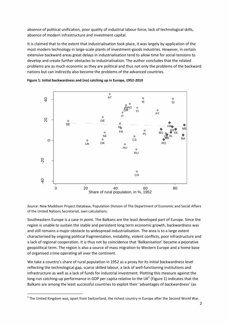
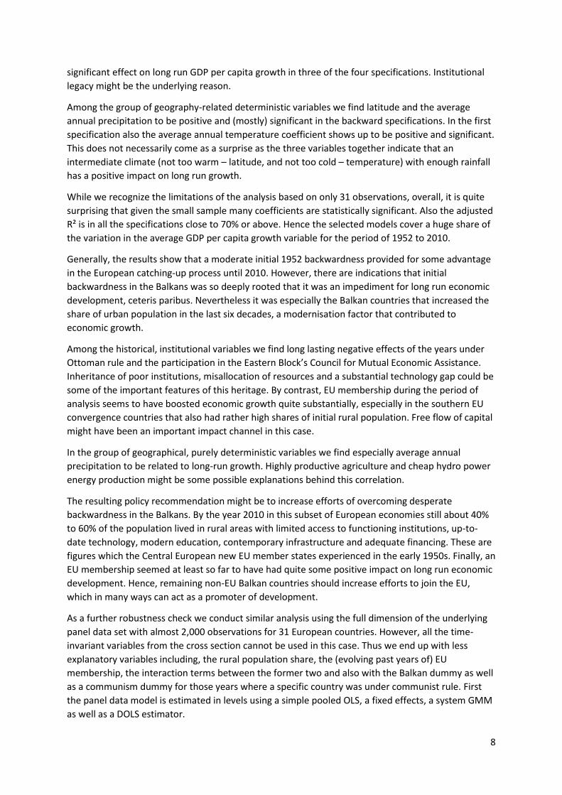
Figure 1: Initial backwardness and (no) catching up in Europe, 1952-2010
Source: New Maddison Project Database, Population Division of The Department of Economic and Social Affairs
of the United Nations Secretariat, own calculations.
Southeastern Europe is a case in point. The Balkans are the least developed part of Europe. Since the
region is unable to sustain the stable and persistent long term economic growth, backwardness was
and still remains a major obstacle to widespread industrialisation. The area is to a large extent
characterised by ongoing political fragmentation, instability, violent conflicts, poor infrastructure and
a lack of regional cooperation. It is thus not by coincidence that ‘Balkanisation’ became a pejorative
geopolitical term. The region is also a source of mass migration to Western Europe and a home base
of organised crime operating all over the continent.
We take a country’s share of rural population in 1952 as a proxy for its initial backwardness level
reflecting the technological gap, scarce skilled labour, a lack of well-functioning institutions and
infrastructure as well as a lack of funds for industrial investment. Plotting this measure against the
long-run catching-up performance in GDP per capita relative to the UK2 (Figure 1) indicates that the
Balkans are among the least successful countries to exploit their ‘advantages of backwardness’ (as
2 The United Kingdom was, apart from Switzerland, the richest country in Europe after the Second World War.
AT
BE
CSDK
FI
FR
DE
GR
HU
IE
IT
NL
NO
PL
PT
RU
SI
ES
SE
CH
TR
UK
ALBA
BG
HR
XK
MK
ME
RO
RS
-40
-20
02
04
0
Cha
ng
e in
GD
P p
er
ca
pita
re
lative to
UK
, in
pp., 1
952
-20
10
0 20 40 60 80Share of rural population, in %, 1952
3
also paraphrased in the more recent literature on long-run development, e.g. Hsiao and Hsiao, 2004).
Some long-established EU member countries with an almost equally backward starting position such
as, for instance, Ireland and Portugal were much more successful in catching up. The generous flow
of EU transfers, the adoption of better institutions, market access and a surge in foreign direct
investment might have been at the basis of their development, which highlights the role of the EU as
a modern promoter of industrialisation.
The theoretical conjecture and descriptive observations hence give rise to the following research
questions we intend to address in the present study:
i) Are the Balkans an extensive backward area with particularly rigid obstacles to economic
development and industrialisation over the long run? ii) What is the general impact of EU
membership on long-term economic development and industrialisation? iii) What are the long-run
industrialisation and deindustrialisation patterns in different sectors in Europe?
We analyse these research questions using econometric methods and a panel dataset that spans six
decades from the mid-20th century up to the early-21st century for up to 31 European countries. The
study is split into two major parts. First, long-run income convergence aspects at the aggregate
country level are examined. Second, the patterns of industrialisation are studied via industry-level
analysis.
2. Backwardness, catching up and economic development
2.1. Literature review The catching-up hypothesis of the exploitation of the ‘advantages of backwardness’ dates back as far
as to the contributions of Veblen (1915) and Gerschenkron (1952). While later contributions mostly
focused on per capita income to depict the level of initial backwardness in the catching up process,
Gerschenkron had a more complex indication of a range of institutional features in mind that more
generally comprises the organisation of agriculture, the extent of urbanisation and the development
of factor markets (Harley, 2015). Here we think that our chosen indicator of the share of rural
population can add multiple dimensions to the concept of backwardness, in addition to the plain GDP
per capita level. Nevertheless, most of the subsequent literature focuses on the later indicator only
and consequently the literature on catching up is also referred to as the ‘income convergence’
literature (Verspagen, 1991).
Empirical literature testing the convergence hypothesis has been mostly constrained by the
availability of reliable data. Early empirical literature such as Abramovitz (1986) and Baumol (1986)
used the Maddison (1982) data base to report some of the first empirical findings on the catching up
hypothesis. Both authors reported convergence based on a sample of advanced countries. On the
other hand, De Long (1988) pointed to the sample selection bias and an inappropriate estimation
strategy in Baumol’s paper, and couldn’t confirm convergence in a wider sample of 22 developed
countries.
Later, Barro and Sala-i-Martin (Barro, 1991; Barro and Sala-i-Martin, 1992) introduced the concept of
conditional convergence - the idea that different economies have different steady states and
pioneering work on testing conditional convergence in cross-country regressions was done in
Mankiw et al. (1992). The paper was also seen as the reinstatement of the neoclassical growth
theory, which was losing ground against the endogenous growth theory at that time. The Mankiw et
4
al. (1992) framework has remained popular in empirical studies on conditional convergence and saw
many extensions including both cross-sectional and panel data analysis.
The panel data approach received significant interest in the literature (see Islam, 1995; Sala-i-Martin,
1996) because it was able to account for heterogeneous country effects along with the time
dimension. Since the existence of endogenous and lagged dependent variables was potentially
causing inconsistent and biased estimates in these specifications, first-difference and system GMM
approaches were later used by many authors (see Caselli et al., 1996; Lee at al., 1998; Bond at al.,
2001), but suffered from the problem of pronounced parameter estimation variation for the same
data set. A predominant number of authors confirmed the conditional convergence hypothesis at
different rates and for different samples. The most commonly found convergence rate was around
2% per year, but there were also some estimates in the range from 4-10% per year. Panel data
approach yields generally a wider range of coefficients compared to cross-section estimates.
The development of non-stationary time series econometrics and the literature on stochastic
convergence in the 1990s as well as the availability of longer data sets made it possible to test the
income convergence hypothesis in the context of time series. This literature first started with the
bivariate unit-root and cointegration tests in small samples (see Bernard and Durlauf, 1995) and
moved to the testing of income convergence in broad samples of countries (Jones, 2002; Pesaran,
2007a) with extensions of the baseline approach were introduced (see Carlino and Mills, 1993; Li and
Pappel, 1999; Strazicich et al., 2004).
In a later stage, the literature developed in the direction of panel data unit root tests (see Levin and
Lin, 1993; Evans and Karras, 1996a; Fleissig and Strauss, 2001) which was followed with the
application of more powerful panel stationarity and cointegration tests (Pedroni, 1999; Maddala and
Wu, 2001; Pesaran, 2007b; see also Hurlin and Mignon, 2007; Phillips and Sul, 2007) that were able
to account for cross-sectional dependence and heterogeneity of the sample became standard in
income convergence testing.
In recent years also a literature on income convergence and its determinants in European transition
countries developed. It can be broadly divided into three strands. The first strand refers to the
analysis of income convergence between the East European countries and the EU and uses the
methodology of sigma and beta regressions (Matkowski and Prochniak, 2004; ECB, 2007; Vojinovic
and Oplotnik, 2008; Vojinovic and Prochniak, 2009; Vojinovic, Acharya and Prochniak 2009; Rapacki
and Prochniak 2009).
The second strand analyses the income convergence of the New EU Member States to the EU income
average by using time series methodology in the bivariate and panel context (Kutan and Yigit, 2004;
Cunado and Grazia, 2006; Brüggermann and Trenkler, 2007; Reza and Zahra, 2008).
The third research strand focuses on the wider aspects of economic convergence of the New
Member States towards European levels and includes monetary as well as real economy variables
(Brada and Kutan, 2001; Brada, Kutan and Zhou, 2002; Backe et al. , 2002; Hermann and Jochem,
2003; Kocenda, 2001; Kocenda, Kutan and Yigit, 2006; Prochniak, 2011).
All of the mentioned papers focus on the post-1995 period, and therefore analyse the transition
process of Eastern European countries, their EU integration or membership effects. This literature
faces estimation problems related to short and small samples, as well as generalisation of results.
There is some evidence of income convergence after the initial transition phase when cross-section
and standard panel data estimators were used. On the other hand, time series estimators were able
to confirm the convergence hypothesis in a much smaller number of cases.
5
Our research therefore adds to the existing convergence literature by analysing historical (longer
than other work) income convergence, economic development processes and the impact of
European Union membership, as well as backwardness, specifically in the Balkans, the poorest region
of Europe.
2.2. Empirical strategy and data issues Our empirical strategy is constrained by data availability as we are predominantly interested in the
long-term impact of economic backwardness and the EU membership effects.
Since most of our variables of interest have low or no time variability, we use a cross-section
approach as our preferred specification and panel data estimations as a robustness check using
pooled ordinary least squares (OLS), fixed effects, generalized method of moments (GMM) and
dynamic OLS (DOLS) estimators with annual data in levels and first differences.
To address the hypothesis of interest and following the convergence literature we consider the
general cross sectional econometric model of the following general form:
∆𝐺𝐷𝑃𝑖 = 𝐺𝑒𝑜𝑔𝑟𝑎𝑝ℎ𝑦′𝑖 + 𝐻𝑖𝑠𝑡𝑜𝑟𝑦′𝑖 + 𝐵𝑎𝑐𝑘𝑤𝑎𝑟𝑑𝑛𝑒𝑠𝑠′𝑖 + 𝐸𝑈′𝑖 + 𝜀𝑖, (1)
where ∆𝐺𝐷𝑃𝑖 is the average annual percentage change of real GDP per capita of country 𝑖 between
the years 1952 (earliest available year for 31 European economies) and 2010 from the 2013 version
of the New Maddison Project Database (for a discussion of the data see Bolt and van Zanden, 2014).
The vector 𝐺𝑒𝑜𝑔𝑟𝑎𝑝ℎ𝑦′𝑖 contains the determinants latitude and longitude of the capital city in
decimal format, the country’s average 1961-1999 annual temperature in degrees Celsius as well as
average annual precipitation in millimetres. Data on the average climatic conditions was taken from
the World Bank’s Climate Change Knowledge Portal.
The vector 𝐻𝑖𝑠𝑡𝑜𝑟𝑦′𝑖 includes a number of explanatory variables that mostly stand for distinctive
institutional and political legacies. These comprise the years under Habsburg (see e.g. Dimitrova-
Grajzl, 2007), years under Ottoman rule, fixed effects for the Habsburg rule in 1800, the Ottoman
rule in 1800, and the Romanov rule in 1800. There are dummy variables for the World War I and
World War II battleground sites, a Yugoslavia 1943, and a Comecon 1949 membership dummy. The
Comecon dummy represents the participation in the Eastern Block’s Council for Mutual Economic
Assistance (Comecon) and hence a substantial period of about five decades of the Soviet-style central
planning. The Yugoslavia membership dummy should indicate whether there was a specific effect of
the Yugoslav Third Way of workers' self-management on the Yugoslav Republics’ long-term growth.
The vector 𝐵𝑎𝑐𝑘𝑤𝑎𝑟𝑑𝑛𝑒𝑠𝑠′𝑖 covers the remaining factors reflecting economic backwardness in the
spirit of Gerschenkron. Among these variables we also include GDP per capita in the year 1952. The
initial income level is used as a control variable for economic convergence in most growth
regressions such as in the seminal papers of Barro (1991) and Levine and Renelt (1992). In order to
capture non-income facets of backwardness we also include the rural population share in 1952 as
provided by the Population Division of The Department of Economic and Social Affairs of the United
Nations Secretariat. The correlation coefficient for these last two variables is at -0.82, which is a
rather high value but not too high to necessarily consider multicollinearity (see also correlation
matrix in Table A2 of the Appendix). Yet, in certain cases these two variables may contain different
information. A case in point being Greece, Norway and Switzerland which had in 1952 about half of
the population still living in rural areas. However, the GDP per capita of Norway was at that time
about triple the level of Greece and in the case of Switzerland this was almost five times the level of
the Hellenic Republic.
6
In order to specifically capture the issue of backwardness in the Balkans we also include a Balkan
dummy (takes the value of unity for Albania, Bosnia and Herzegovina, Bulgaria, Croatia, Kosovo,
Macedonia, Montenegro, Romania and Serbia), as well as an interaction term of the Balkan with the
rural population share in 1952 (for better interpretation interacted data is centred). This variable
should capture whether there is something specific about the initial level of Balkan backwardness
that is stronger than Gerschenkron’s moderate backwardness that can be exploited as an advantage
in the growth catch-up. In this group of variables we also consider the urbanisation share change
between 1952 and 2010 in percentage points, in order to see whether efforts of modernisation are
being rewarded by faster development in the analysed sample of 31 European countries.
Finally in the 𝐸𝑈′ vector there is both an EU dummy and the membership years in the EU, both of
which are of special interest. Both are also interacted with the rural population share in order to find
out how EU membership has affected backward countries. Summary statistics for all the variables
employed can be found in Table A1 of the Appendix.
A number of the most backward European economies did not have any substantial economic
development even decades before the 1950s. This suggests the possibility that the rural population
share is not a fully exogenous variable. Hence there might be the issue that Southeast Europe’s
dependence on low-productivity agriculture was not a cause, but a consequence of
underdevelopment (see Kopsidis, 2012). Also, if the rural population share is to be interpreted as a
proxy for more general institutional conditions, recent literature assumes here a certain degree of
endogeneity as well (see e.g. Acemoglu et al. 2001, 2012). Moreover, it is suggested that geography
(e.g. Bleaney and Dimico, 2010) and climate (e.g. Dell et. al. 2009) are important factors. However,
formal tests of the rural population share indicate it can be treated as an exogenous variable in our
specification.
Given the small sample size at hand we need to economise on the number of explanatory variables.
Therefore different variable selection procedures are being employed, which also serves as a
robustness check. We made use of a backward selection procedure where the significance level for
removal from the model was chosen at 10%. Second, a forward selection was employed with a
significance level for addition to the model of 10%. Finally, a backward stepwise and a forward
stepwise selection procedure was used. In both cases the significance level for removal from the
model is 10% and for addition to the model 9%. The results of these cross-section estimations can be
found in Table 1.
2.3. Discussion of the results The forward specifications yield same results, while the backward specifications have slightly
different coefficients and significance levels. The Balkan rural 1952 population share interaction term
is only significant at the 5% level in the backward selection and stepwise specifications. The
coefficient has a negative sign, which hints at the possibility that the Balkan-specific backwardness
was ceteris paribus an obstacle for subsequent economic development of the region. The Balkan
dummy was nowhere found to be significant and the rural population share for all the countries in
1952 is only significant and interestingly also negative in the first specification only. However, it is
also only in the backward selection specification that the urbanisation share change variable is
significant and positive, which hints at the gains from actively overcoming backwardness.
However, statistical significance is much stronger in the case of the remaining indicator related to
backwardness. In all the specifications the log of initial GDP per capita is negative significant at the
1% level. This could be interpreted as an ‘advantage of backwardness’ at least for the countries
7
outside the Balkans that were poor in 1952 but had fairly low shares of rural population – thus some
sort of ‘moderate backwardness’.
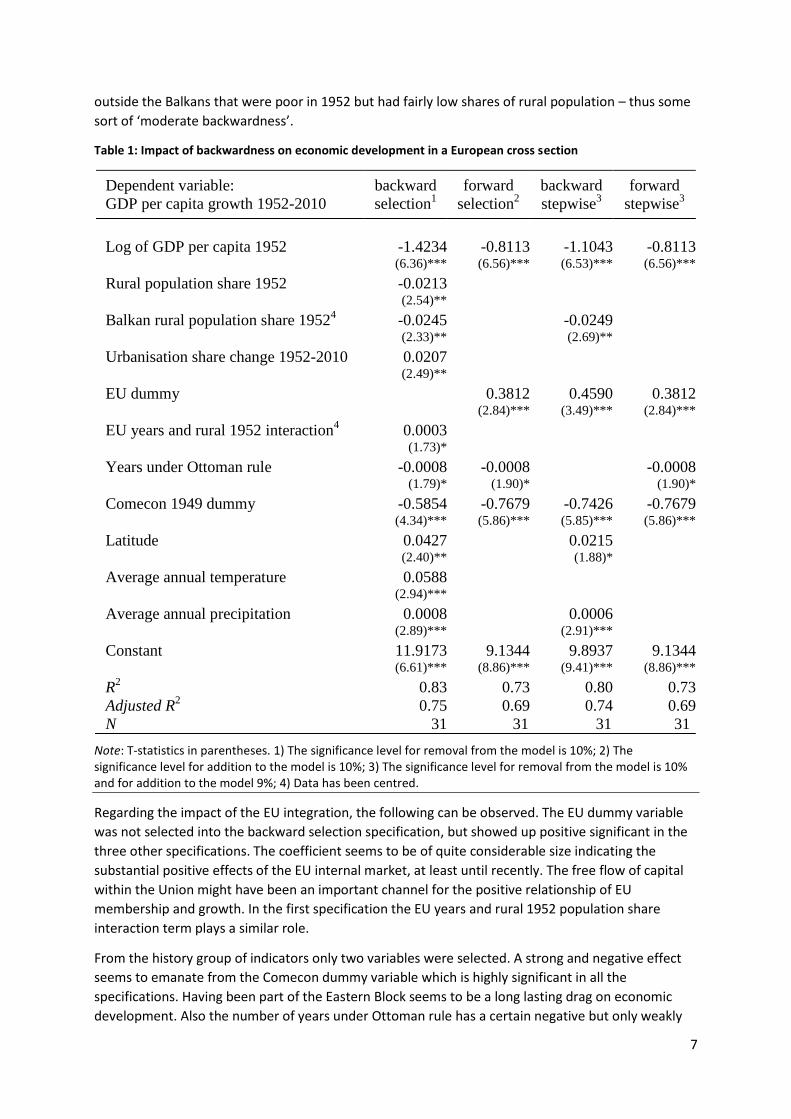
Table 1: Impact of backwardness on economic development in a European cross section
Dependent variable:
GDP per capita growth 1952-2010
backward
selection1
forward
selection2
backward
stepwise3
forward
stepwise3
Log of GDP per capita 1952 -1.4234 -0.8113 -1.1043 -0.8113
(6.36)*** (6.56)*** (6.53)*** (6.56)***
Rural population share 1952 -0.0213
(2.54)**
Balkan rural population share 19524 -0.0245 -0.0249
(2.33)** (2.69)**
Urbanisation share change 1952-2010 0.0207
(2.49)**
EU dummy 0.3812 0.4590 0.3812
(2.84)*** (3.49)*** (2.84)***
EU years and rural 1952 interaction4 0.0003
(1.73)*
Years under Ottoman rule -0.0008 -0.0008 -0.0008
(1.79)* (1.90)* (1.90)*
Comecon 1949 dummy -0.5854 -0.7679 -0.7426 -0.7679
(4.34)*** (5.86)*** (5.85)*** (5.86)***
Latitude 0.0427 0.0215
(2.40)** (1.88)*
Average annual temperature 0.0588
(2.94)***
Average annual precipitation 0.0008 0.0006
(2.89)*** (2.91)***
Constant 11.9173 9.1344 9.8937 9.1344
(6.61)*** (8.86)*** (9.41)*** (8.86)***
R2 0.83 0.73 0.80 0.73
Adjusted R2 0.75 0.69 0.74 0.69
N 31 31 31 31
Note: T-statistics in parentheses. 1) The significance level for removal from the model is 10%; 2) The significance level for addition to the model is 10%; 3) The significance level for removal from the model is 10% and for addition to the model 9%; 4) Data has been centred.
Regarding the impact of the EU integration, the following can be observed. The EU dummy variable
was not selected into the backward selection specification, but showed up positive significant in the
three other specifications. The coefficient seems to be of quite considerable size indicating the
substantial positive effects of the EU internal market, at least until recently. The free flow of capital
within the Union might have been an important channel for the positive relationship of EU
membership and growth. In the first specification the EU years and rural 1952 population share
interaction term plays a similar role.
From the history group of indicators only two variables were selected. A strong and negative effect
seems to emanate from the Comecon dummy variable which is highly significant in all the
specifications. Having been part of the Eastern Block seems to be a long lasting drag on economic
development. Also the number of years under Ottoman rule has a certain negative but only weakly
8
significant effect on long run GDP per capita growth in three of the four specifications. Institutional
legacy might be the underlying reason.
Among the group of geography-related deterministic variables we find latitude and the average
annual precipitation to be positive and (mostly) significant in the backward specifications. In the first
specification also the average annual temperature coefficient shows up to be positive and significant.
This does not necessarily come as a surprise as the three variables together indicate that an
intermediate climate (not too warm – latitude, and not too cold – temperature) with enough rainfall
has a positive impact on long run growth.
While we recognize the limitations of the analysis based on only 31 observations, overall, it is quite
surprising that given the small sample many coefficients are statistically significant. Also the adjusted
R² is in all the specifications close to 70% or above. Hence the selected models cover a huge share of
the variation in the average GDP per capita growth variable for the period of 1952 to 2010.
Generally, the results show that a moderate initial 1952 backwardness provided for some advantage
in the European catching-up process until 2010. However, there are indications that initial
backwardness in the Balkans was so deeply rooted that it was an impediment for long run economic
development, ceteris paribus. Nevertheless it was especially the Balkan countries that increased the
share of urban population in the last six decades, a modernisation factor that contributed to
economic growth.
Among the historical, institutional variables we find long lasting negative effects of the years under
Ottoman rule and the participation in the Eastern Block’s Council for Mutual Economic Assistance.
Inheritance of poor institutions, misallocation of resources and a substantial technology gap could be
some of the important features of this heritage. By contrast, EU membership during the period of
analysis seems to have boosted economic growth quite substantially, especially in the southern EU
convergence countries that also had rather high shares of initial rural population. Free flow of capital
might have been an important impact channel in this case.
In the group of geographical, purely deterministic variables we find especially average annual
precipitation to be related to long-run growth. Highly productive agriculture and cheap hydro power
energy production might be some possible explanations behind this correlation.
The resulting policy recommendation might be to increase efforts of overcoming desperate
backwardness in the Balkans. By the year 2010 in this subset of European economies still about 40%
to 60% of the population lived in rural areas with limited access to functioning institutions, up-to-
date technology, modern education, contemporary infrastructure and adequate financing. These are
figures which the Central European new EU member states experienced in the early 1950s. Finally, an
EU membership seemed at least so far to have had quite some positive impact on long run economic
development. Hence, remaining non-EU Balkan countries should increase efforts to join the EU,
which in many ways can act as a promoter of development.
As a further robustness check we conduct similar analysis using the full dimension of the underlying
panel data set with almost 2,000 observations for 31 European countries. However, all the time-
invariant variables from the cross section cannot be used in this case. Thus we end up with less
explanatory variables including, the rural population share, the (evolving past years of) EU
membership, the interaction terms between the former two and also with the Balkan dummy as well
as a communism dummy for those years where a specific country was under communist rule. First
the panel data model is estimated in levels using a simple pooled OLS, a fixed effects, a system GMM
as well as a DOLS estimator.

9
The last one is our preferred model as (according to Kao and Chiang, 2001) it is the most appropriate
estimator for potentially non-stationary level data that may represent a long-run cointegrated
relationship. However, it is unclear whether our GDP and rural population data is really non-
stationary or not (about half of the different tests available show either result). Nevertheless,
allowing each country to have its own short-run dynamic interactions and feedbacks (here we use
one lead and two lags of the first differences) should give consistent estimates of the parameters
that are also robust to reverse causality.
Table 2: Impact of backwardness on economic development in a European panel data setting
Dependent variable:
GDP per capita 1952-2010 OLS FE SYS-GMM DOLS
Rural population share -0.0307 -0.00945** -0.00967* -0.0103**
(0.0276) (0.00416) (0.00551) (0.00457)
Balkan rural population share 0.0592 -0.00131 0.000869 -0.00286
(0.0369) (0.00453) (0.00121) (0.00453)
EU dummy and rural interaction 0.0184 0.00561** -0.00179* 0.00481**
(0.0274) (0.00212) (0.00103) (0.00235)
EU dummy 1.114*** 0.184*** -0.000453 0.175***
(0.316) (0.0381) (0.00870) (0.0376)
EU dummy and Balkan
interaction
-0.400 -0.215*** 0.00279 -0.126**
(0.559) (0.0573) (0.0125) (0.0581)
Yugoslavia dummy -3.380** 0.311** 0.0521* 0.338**
(1.402) (0.119) (0.0259) (0.124)
Comecon dummy -0.282 0.324*** 0.0172 0.283***
(0.533) (0.0869) (0.0241) (0.0942)
Lagged log of GDP per capita 0.822***
(0.0913)
Constant 9.572*** 7.945*** 1.062***
(1.166) (0.214) (0.235)
Observations 1,829 1,829 1,767 1,736
R-squared 0.430 0.902 0.995
Number of countries 31 31 31 31
Note: Robust standard errors in parentheses. Interaction data has been centred. Like the FE specification, DOLS
includes fixed country and time effects.
Simply taking first differences of all the variables, to eliminate non-stationarity, results in an
estimation that may fail to capture the long-run relationship in levels that is at the heart of this
analysis. Nevertheless we have also estimated specifications in first differences (see Tables A4 and A5
in the Appendix), which however do not result in very different outcomes. Also, we have used for
levels as well as first differences system GMM and first differenced GMM, respectively. The
coefficients of these estimates are often insignificant though and in any case the GMM methodology
is being used for panels with a ‘large N and small T’, which is not the case with our panel.
The results (Table 2) portray a picture quite similar to the one from the cross-section estimations.
Backwardness, as indicated by the share of the rural population, seems to be impeding economic
development. On the other hand, membership in the European Union seems to be favourable,
especially for those countries that are quite backward. The coefficient of the interaction term of EU
10
membership and the Balkan dummy is negative. In the specifications where we use EU membership
years instead of the EU dummy (see Appendix Table A3) that coefficient is insignificant altogether.
However, given that Romania and Bulgaria are the only Balkan countries that joined the EU until
2010 (both in 2007) we have only eight non-zero observations for this variable for the period of the
global financial crisis which makes it less reliable. Interestingly, the coefficients of both communism
dummies (Yugoslavia and Comecon) are positive significant in all the DOLS specifications.
Overall, the panel data approach seems to support the main insight from the cross section. It appears
that the EU is a promoter of economic development especially in backward countries. The
observation that the Balkans are an extensive backward area with substantial impediments to
economic development can only be confirmed in the first differences fixed effects models and can
hence not be seen as perfectly robust.
In the next chapter we shift the focus from the macro to the industry level. The implications of
(Balkan) backwardness and the EU membership are analysed with the help of data for different
manufacturing industry sectors for different periods.
3. Industrialisation and economic development
3.1. Literature review While in the early literature such as in Veblen (1915), Gerschenkron (1952) or Rosenstein-Rodan
(1943) industrialisation was almost seen synonymous to economic development, later literature used
the term increasingly to convey the rising manufacturing sector. In the 1980s, a period of fascination
with the service sector has set in and soon industrial policy earned a bad name due to many cases of
large, selective and often ill-designed backward-looking subsidies to ailing firms and sunset industries
in the 1960s and 1970s (Crafts, 2010). However, in the wake of the global financial crisis a return of
industrial policy (Wade, 2012) and even a ‘European Industrial Renaissance’ (EC, 2014) have been
proclaimed. De-industrialisation is being widely complained of and re-industrialisation is being
propagated, though not without critique (Ambroziak, 2014).
The debate is closely related to concerns about loss of employment, trade imbalances and sluggish
technological development in advanced economies, as well as doubts about the development model
and premature deindustrialisation in transition and emerging economies. The revival of interest for
the manufacturing sector can also be seen as related to rising scepticism about the role of services as
the main driver of economic growth, the prevailing view over the last three decades. The prime
example of the switch towards manufacturing can be seen in recent state interventions in the
automotive industry or government policies aimed towards preserving a strong manufacturing basis
at the national level.
It has long been acknowledged by classical development economists (Hirschman, Prebisch and
Kaldor) that industrialization plays an important role for economic growth (see also Peneder, 2003;
Rodrik, 2009; and Szirmai and Verspagen, 2011). This is not surprising given that manufacturing is
seen as a major source of technological progress and as a high productivity growth sector (Stöllinger
et al., 2013). Furthermore, capital accumulation seems to be faster and more intense in
manufacturing than in other sectors (Cruz, 2015). Felipe, Mehta, and Rhee (2014) point to the
economies of scale in the manufacturing sector that don’t exist in other sectors and that
technological development and diffusion towards other sectors starts from manufacturing. Linkage
and spillover effects seem to be strongest in the manufacturing sector (Tregenna, 2009). Moreover,

11
manufacturing offers greatest opportunities for raising the exporting potential of the economy
(Pacheco and Thirlwall, 2013), which might be important in order to profit from expanding global
markets.
Since there has been no unanimous consensus about the precise definition, many different empirical
proxies for industrialisation are present in the literature, the most common ones being the change in
manufacturing employment and manufacturing output shares. Liu and Li (2015) stress that relying on
these measures only underscores the multidimensionality of structural change related to
(de-)industrialisation. They suggest a way to merge economic growth literature with empirics of
industrialisation where they regress the following vector of dependent variables: GDP growth,
agriculture, and industry and service sector shares in GDP as well as output growth rates of these
three sectors on a set of 43 control variables. The analysis uses a global sample of 164 countries in
the period of 1970 to 2010 and comes up with some important findings. The variables used to
explain GDP growth can also explain sector shares and growth with similar explanatory power but
different independent variables have a varying impact on each dependent variable. Some
independent variables have consistent effects, while others exhibit variable effects on growth and
sectoral shares. Their empirical results generally support the link between economic growth and
industrialisation.
Tregenna (2009) addresses the complexity aspects of deindustrialisation as well, stressing that (de-
)industrialisation should be defined as a concomitant (fall) increase in the share of manufacturing in
total employment and the share of manufacturing value added in GDP. Focusing on the
manufacturing share in total employment only would therefore undermine the importance of
distinguishing different patterns of deindustrialisation. The paper suggests a decomposition of
changes in levels and shares of manufacturing employment into components related to changes in
the share of manufacturing value added in GDP, growth of manufacturing value-added, labour
intensity of manufacturing production and economic growth. The results, on the data sample of 48
countries for a period from 1980 to 2003 (but shorter for some countries due to data availability),
show that the globally observed manufacturing employment fall is dominantly related to declining
labor intensity, i.e. ratio of employment to value-added, in manufacturing as opposed to an overall
decline in the size or share of the manufacturing sector.
Besides definition issues, empirical growth literature was mostly concerned with the impact (de-
)industrialisation has on economic growth and/or its determinants. Szirmai (2012) stresses the
historical importance of manufacturing for economic growth. His results, on a sample of 67
developing and 21 rich countries in the period 1950 to 2005, show that manufacturing was especially
beneficial to successful Asian countries and partly explains the disappointing performance of some
African countries. Similar to that, Rodrik (2015) documents worldwide deindustrialisation trends for
42 countries in the period from the 1950s to the 2010s, where his dependent variables are
manufacturing employment as well as output shares, in current and real prices. The results point to
globalisation and trade as factors driving the diverging patterns of successful Asian and prematurely
deindustrialised Latin American countries whereas labour saving technological progress can well
explain concomitant manufacturing employment loss and fairly well manufacturing output
performance in advanced economies.
Building on a neoclassical model, Nickell, Redding and Swaffeld (2008) develop an empirical approach
that allows them to decompose the deindustrialisation process into contributions of prices,
technology and factor endowments. Several findings, based on a sample of 14 OECD countries and
industries for the period 1975 to 1994, emerge from their analysis. The fast decline in the
manufacturing to GDP share in the UK and USA relative to Germany and Japan can be explained by
12
productivity growth and the relative price changes of manufacturing and nonmanufacturing goods.
Decline in the agricultural sector share of GDP in Italy and Japan depends on productivity growth and
relative price movements. Different education endowments explain well why the share of services in
GDP had differential growth patterns in OECD countries.
Palma (2008) identifies a few major global sources of manufacturing employment shrinkage. The first
is that the share of manufacturing declines as the economy moves to a more developed stage.
Second, the level of income per capita at which deindustrialisation starts in developing countries is at
a lower level than in early industrialisers. Lastly, there might be a set of other factors, ranging from
policy issues to resource discovery, which can affect deindustrialisation processes.
The effects of trade on deindustrialisation are analysed in Rowthorn and Coutts (2004). Their results,
in a sample of 23 OECD countries for the period 1963 to 2002, point to trade being a stronger driver
of deindustrialisation in the North than in the South. Interestingly, the analysis finds that domestic
factors have generally a stronger impact on deindustrialisation than trade. That result is similar to the
one in Cruz (2015) whose results confirm the importance of income per capita, domestic income
distribution, labour manufacturing productivity and capital accumulation, i.e. of domestic factors on
deindustrialisation in Mexico. The weak impact of trade on deindustrialisation is also confirmed in an
earlier paper of Rowthorn and Ramaswamy (1997) that uses a smaller sample of 18 OECD countries
in the period 1963 to 1994. Their results show that the faster relative productivity growth in
manufacturing as compared to the services sector explains the manufacturing employment
shrinkage. It is interesting to note that the authors don’t consider deindustrialisation as a negative,
but rather a natural consequence of economic development. Contrasting results can be found in
Kucera and Milberg (2003) who use input-output analysis in a sample of 10 OECD economies for the
period of the 1970s to the 1990s to show that the manufacturing employment decline is mainly due
to North-South trade.
The literature about the determinants of the long term industrialisation process in transition
economies has been scarce and is mostly related to country case studies. Comparative research that
focused on the Balkan countries has been missing as well. However, in the case of the Balkan
economies, some of which never had experienced extensive industrialisation, it is to a large extent
undisputed that (similarly to the recommendations of Rosenstein-Rodan in 1943) industrialisation is
the key to sustainable economic development. In the following we want to find out whether there
are specific Balkan obstacles to industrialisation and whether the European Union membership can
act as a promoter of industrialisation. All of that we want to investigate for different types of
industries and different time periods in order to learn more about sector and time specific patterns.
3.2. Empirical strategy and data issues Our empirical strategy combines several approaches used in the relevant industrialisation literature:
i) It makes use of a simple, but powerful baseline specification employed by Rajan and Subramanian
(2011) for manufacturing growth at the industry level; ii) We acknowledge in the choice of our
dependent variables the complexity of industrialisation as emphasised by Tregenna (2009); iii)
Finally, we also distinguish industrial sectors by stage of development as defined in Haraguchi (2014).
According to Haraguchi (2014), it is likely that the pattern of transformation induced by technological
changes, economic integration, institutional convergence and other factors is likely to differ across
industries depending on their technological sophistication. Hence developing nations should have a
higher propensity to specialise in labour-intensive industries, while advanced economies, conversely,
should tend to transform to more technology-intensive industries. Therefore, following Haraguchi
13
(2014), we split all manufacturing industries into three categories: early, middle and late industries.
Note that this is opposite to the historical observations of Gerschenkron (1952) that industrialisation
took place largely by application of the most modern technology in large-scale plants of investment-
goods industries.
We measure industrialisation in a number of different ways for robustness, as suggested in Tregenna
(2009). In particular, we incorporate indicators based on sectoral value added and employment data
to measure the degree of industrialisation. This includes the employment growth as well as the
change in the employment share, the value added growth as well as the change in the value added
share and in addition also labour productivity. Defining industrialisation in a traditional way (that is,
in terms of employment share) is conceptually limiting given that some of the Kaldorian processes
operate primarily through output rather than employment. Hence we use several measures of
industrialisation based on employment and value added data for extra robustness. Tregenna (2009)
emphasises that from a Kaldorian perspective industrialisation could have substantial implications for
long-run growth, given the special growth-pulling properties of manufacturing (Kaldor, 1966, 1967).
Thus the empirical strategy focuses on identifying the industry-level developments in the context of
backwardness and European integration over a long time horizon differentiating between types of
industries. In particular, the following specification, based on the Rajan and Subramanian (2011)
approach, is used:
𝛥10𝑌𝑎𝑣𝑔𝐼𝑛𝑑𝑢𝑠𝑡𝑟𝑖𝑎𝑙𝑖𝑠𝑎𝑡𝑖𝑜𝑛𝑖𝑐 = 𝐼𝑛𝑖𝑡𝑖𝑎𝑙𝑖𝑐𝑡=0 + 𝐹𝐸′𝑖𝑐 + 𝐼𝑛𝑡𝑒𝑟𝑎𝑐𝑡𝑖𝑜𝑛′𝑖𝑐 + 𝜀𝑖𝑐 , (2)
where the subscripts 𝑖 and 𝑐 represent 2-digit ISIC Revision 3 industries and countries, respectively.
We use several measures of industrialisation, as previously described, to capture various aspects of
the phenomenon (10-year average annual growth values), defined for each 2-digit ISIC industry:
A) Average change in industry 𝑖 value added as a share of GDP;
B) Average growth of real value added of industry 𝑖;
C) Average change in industry 𝑖 employment as a share of total country employment;
D) Average growth of employment in industry 𝑖;
E) Average growth of labour productivity in industry 𝑖, defined as the ratio of real value added to
employment in industry 𝑖.
Given the maximum available time dimension of the industry and GDP data the following five periods
are used: 1963-1972, 1973-1982, 1983-1992, 1993-2002, and 2003-2011. Averages for industry data
available for seven or more years were used. Information for industries with less than 7 observations
per period of analysis was not employed. In addition, we analyse the longest period available for as
many countries as possibly: 1965-2011.
The vector of fixed effects, 𝐹𝐸′𝑖𝑐 includes country and industry fixed effects. 𝐼𝑛𝑖𝑡𝑖𝑎𝑙𝑖𝑐𝑡=0 denotes the
initial conditions at the first year of the respective 10-year period, and is manufacturing value added,
in % of GDP for the specifications (A), (B), initial manufacturing employment share for specifications
(C) and (D), and the initial labour productivity for specification (E). Its coefficient thus reflects the
speed of convergence.
We also introduce the vector 𝐼𝑛𝑡𝑒𝑟𝑎𝑐𝑡𝑖𝑜𝑛′𝑖𝑐, containing interaction terms between industry stage
dummy variables (early, middle and late industries) and each of the following: EU membership,
Communist, Balkans dummy variables. The ‘Balkans’ dummy variable takes the value of unity for the
following countries: Albania, Bosnia and Herzegovina, Bulgaria, Croatia, Kosovo, Macedonia,
14
Montenegro, Romania, Serbia, and, for earlier periods, Yugoslavia. The countries included in the
group share similar transition experience and historical background. The ‘Communist’ dummy
variable takes the value of unity for countries which are communist (for the pre-1990 periods) or
were communist in the past (for the periods post-1990). The ‘EU membership’ dummy variable takes
the value of unity if a country is or becomes an EU member within the corresponding decade.
In addition, we introduce three interaction terms with 𝐵𝑎𝑐𝑘𝑤𝑎𝑟𝑑𝑖𝑐𝑡=0 - our ‘backwardness’ variable,
measured as rural population as a percentage of total population at the beginning of the respective
decade (t=0), and capturing the extent to which initial backwardness matters for the pace of
industrialisation over the course of the following decade for each of the industry groups. The industry
stage dummy variables, early, middle and late, take the value of unity if an industry belongs to an
‘early-‘, ‘middle-’ or ‘late-stage’ industry group defined according to Haraguchi (2014) as follows:
Early-stage industries comprise the sectors of Food and beverages, Tobacco, Textiles,
Wearing apparel, Wood products, Publishing, Furniture, Non-metallic minerals (i.e. the ISIC
Rev.3 industries: 15, 16, 17, 18, 19, 20, 22, 26, 36);
Middle-stage manufacturing includes Coke and refined petroleum, Paper, Basic metals,
Fabricated metals (i.e. ISIC sectors: 21, 23, 27, 28);
Late-stage sector group consists of Rubber and plastic, Motor vehicles, Chemicals, Machinery
and equipment, Electrical machinery and apparatus, Precision instruments (i.e. ISIC
manufacturing industries: 24, 25, 29, 30, 31, 32, 33, 34, 35, 37).
The early-stage industries are labour-intensive and/or domestic-oriented industries. The middle-
stage industries process natural resources to be used by industries further down the value-added
chain. Late-stage industries are relatively more technology-intensive and in most cases produce
output for final use by firms and households.
𝜀𝑖𝑐 denotes the error term. We use standard errors clustered by country.
The panel dataset used in the study spans the period of 1963-2011 and includes a maximum of 43
European countries (including faded countries, such as Czechoslovakia, GDR, Yugoslavia and USSR).
The dataset is constructed using United Nations Industrial Development Organization (UNIDO) and
Penn World Table (PWT) databases. Industry-level data (value added, employment) at the 2-digit
level of ISIC Revision 3 were obtained from the UNIDO INDSTAT database. Country GDP,
employment, deflators were obtained from the Penn World Table 8.1 (for details, see Feenstra et al.,
2015). Rural population share was computed using the data from the Population Division of The
Department of Economic and Social Affairs of the United Nations Secretariat database.
The measure of industrialisation relies on the various indicators of industry-level value added and
employment which allows us to better capture industrialisation or deindustrialisation, as, e.g.
industry value added may increase as a result of labour productivity gains or higher employment. We
use value added rather than output data as it excludes the value of intermediate inputs and
therefore represents a more accurate measure of manufacturing activity. In order to make the value
added data (expressed in nominal USD) consistent with the real GDP data used in the analysis (PPP-
adjusted production-side GDP from the PWT 8.1), we deflate the value added data using the GDP
deflator used to construct the PWT real GDP series, which is equivalent to computing nominal GDP
series). To aid economic interpretation of the corresponding interaction terms the backwardness
variable (share of rural population) is centred by demeaning, and thus the magnitudes of the
respective interaction effects should be interpreted as elasticities at the sample mean.
15
3.3. Discussion of the results
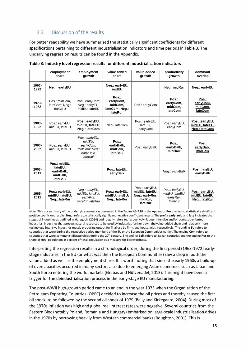
For better readability we have summarised the statistically significant coefficients for different
specifications pertaining to different industrialisation indicators and time periods in Table 3. The
underlying regression results can be found in the Appendix.
Table 3: Industry level regression results for different industrialisation indicators
employment share
employment growth
value added share
value added growth
productivity growth
dominant overlap
1963-1972
Neg.: earlyEU Neg.: earlyEU,
midEU Neg.: midRur Neg.: earlyEU
1973-1982
Pos.: midCom, lateCom; Neg.:
earlyEU
Pos.: earlyCom; Neg.: earlyEU, midEU, lateEU
Pos.: earlyCom, midCom,
lateCom; Neg.: lateRur
Pos.: earlyCom
Pos.: earlyCom, midCom, lateCom
Pos.: earlyCom, midCom, lateCom
1983-1992
Pos.: earlyEU, midEU, lateEU
Pos.: earlyEU, midEU, lateEU; Neg.: lateCom
Neg.: lateCom Pos.: earlyEU,
lateEU, earlyCom
Pos.: earlyEU, earlyCom
Pos.: earlyEU, midEU, lateEU; Neg.: lateCom
1993-2002
Pos.: earlyEU, midEU, lateEU
Pos.: earlyEU, midEU,
earlyCom, midCom; Neg.:
earlyBalk, lateBalk
Pos.: earlyBalk, midBalk, lateBalk
Pos.: earlyBalk Pos.:
earlyBalk, midBalk
Pos.: earlyBalk, midBalk
2003-2011
Pos.: midEU, lateEU,
earlyBalk, midBalk, lateBalk
Pos.: lateEU,
earlyBalk Neg.: earlyBalk
Pos.: lateEU, earlyBalk
1965-2011
Pos.: earlyEU, midEU, lateEU; Neg.: lateRur
Neg.: earlyEU, midEU, lateEU,
earlyRur, midRur, lateRur
Pos.: earlyEU, midEU, lateEU; Neg.: lateRur
Pos.: earlyEU, midEU, lateEU; Neg.: earlyRur,
midRur, lateRur
Pos.: earlyEU, midEU, lateEU,
earlyRur, lateRur
Pos.: earlyEU, midEU, lateEU; Neg.: lateRur
Note: This is a summary of the underlying regression presented in the Tables A6-A10 in the Appendix. Pos.: refers to statistically significant positive coefficient results. Neg.: refers to statistically significant negative coefficient results. The prefix early, mid and late indicates the stages of industries as outlined in Haraguchi (2014) and roughly refers to, respectively, labour intensive and/or domestic-oriented industries, industries that process natural resources to be used by industries further down the value-added chain and relatively more technology-intensive industries mostly producing output for final use by firms and households, respectively. The ending EU refers to countries that were during the respective period members of the EU or the European Communities earlier. The ending Com refers to countries that were communist dictatorships during the 20th century. The ending Balk refers to Balkan countries and the ending Rur to the share of rural population in percent of total population as a measure for backwardness.
Interpreting the regression results in a chronological order, during the first period (1963-1972) early-
stage industries in the EU (or what was then the European Communities) saw a drop in both the
value added as well as the employment share. It is worth noting that since the early 1960s a build-up
of overcapacities occurred in many sectors also due to emerging Asian economies such as Japan and
South Korea entering the world markets (Grabas and Nützenadel, 2013). This might have been a
trigger for the deindustrialisation process in the early-stage EU manufacturing.
The post-WWII high-growth period came to an end in the year 1973 when the Organization of the
Petroleum Exporting Countries (OPEC) decided to increase the oil prices and thereby caused the first
oil shock, to be followed by the second oil shock of 1979 (Baily and Kirkegaard, 2004). During most of
the 1970s inflation was high and global real interest rates were negative. Several countries from the
Eastern Bloc (notably Poland, Romania and Hungary) embarked on large-scale industrialisation drives
in the 1970s by borrowing heavily from Western commercial banks (Boughton, 2001). This is
16
reflected in our regression results for the period 1973-1982. All the three types of industries (early,
middle and late) have experienced increases in the value added share as well as in productivity and
partly also in the employment share.
n the early 1980s the new Chairman of the Federal Reserve Paul Volcker hiked the federal funds rate
in order to fight inflation. Several of the Eastern Bloc countries had been highly indebted and under
the new circumstances found themselves unable to roll over and repay their foreign debt. At the
same time oil prices started to drop dramatically, which caused major problems for the Soviet
economy, the main market for exports from other Comecon members. As a consequence, our
regression results reflect a negative change in late-stage manufacturing value added shares as well as
negative employment growth in these industries in the Communist countries. For the Western
European countries falling oil prices were helpful, which also manifests in the regression results for
the decade as positive growth of employment and employment shares in all three types of industries
in the countries of the European Communities in the period 1983-1992. This is partly also true for
value added and productivity growth.
From March 1989 to April 1992 a revolutionary wave terminated the Communist rule in Central,
Eastern and Southeastern Europe. The simultaneous break-up of Yugoslavia was accompanied by a
series of wars, the most bloody of which ended in 1995. Afterwards the region saw a certain recovery
of industrial production. Our regressions for the period 1993-2002 include now enough Balkan
countries (Albania, Bulgaria, Croatia, Macedonia, Romania) in order to have in addition to the other
interactions also a Balkan dummy and industry stages interaction term. Indeed, especially early-stage
(and partly also medium and late) Balkan industries experienced re-industrialisation with increasing
value added shares, rising value added and productivity growth over this decade. However, at the
same time, early- and late-stage Balkan industries experienced a drop in employment. This hints at
the fact that most of the Balkan economies generally experienced a rather restrained and bumpy
recovery throughout the late 1990s accompanied by a banking crisis, the Kosovo war (1998-1999),
and, later on, the 2001 insurgency in Macedonia. It was a period of ‘jobless growth’.
From 2003 up to 2007 a global growth spurt was also carrying away the Balkans. As a result, for the
regressions over the period 2003-2011 we find a positive development for the early-stage Balkan
industries in terms of value added shares as well as employment shares (productivity growth was on
the decline). Interestingly, also the late-stage EU industry sectors experienced both value added
share and employment share growth during that period. This is probably related to favourable
demand developments in the emerging markets for Western European high-end final manufacturing
goods even after the outbreak of the global financial crisis due to ongoing high commodity prices
supporting many emerging economies for a few more years.
Finally, in the long term regression for the period 1965-2011 results are fairly uniform. Across all
industries of the EU member states we find positive results in terms of employment and value added
share change as well as value added growth. It seems that the main channel was the rise in the
respective productivity growth rates as employment growth was negative in the EU countries’
industries. However, the major shortcoming of this regression is the fact that in the sample there is
only one country that did not become a member of the EU and that is Norway. Interestingly, late-
stage industries in the more rural areas of the European continent experienced negative employment
and value added growth as well as declines in employment and value added shares. This points at
extensive backwardness in countries that were not able to industrialise in the Gerschenkron style by
application of the most modern technology in large-scale plants of investment-goods industries.
As a robustness check we also run all the industry level regressions with the years of EU membership
instead of the EU membership dummy, which yields similar results (see Tables A11-A16 in the

17
Appendix). EU industries experienced a downturn in the 1960s. Communist countries had a period of
industrialisation in the 1970s and a period of deindustrialisation in the 1980s. In the 1980s we find a
divergent pattern for the EU industries now weighted by years of EU membership as compared to
the earlier EU dummy. Industries in then old EU Member States had a period of deindustrialisation
while at that time Southern countries joined the EU which apparently have had a phase of
industrialisation. We also observe for the 1990s and 2000s a post-war recovery, especially for lower-
tech industries in the Balkans. Finally, in the long-term regression for the full time period since the
mid-1960s we find an overall positive effect of a long-lasting EU membership on the industrialisation
of the economy. In some specifications also the long-run deindustrialisation process in backward
economies is confirmed.
4. Conclusions
Southeastern Europe is comprised of the poorest and the most ‘backward’ countries of Europe in
terms of political unification, stable labour force, sufficient technological skills, adequate
infrastructure and available investment capital, as defined by Gerschenkron (1952). Excessive levels
of backwardness could be a major obstacle for economic development and industrialisation in the
region. Other countries that initially had similar levels of backwardness half a century ago, but
became members of the European Union and benefited from generous EU transfers, the adoption of
better institutions, market access and inflow of foreign direct investment have taken a different
development path, suggesting the important role that the EU played as a promoter of long-term
development and industrialisation. We explore these hypotheses in the present paper via cross
section and panel data analysis based on the long-term economic development and industrialisation
data over the period 1952-2010 in Europe, which has become available recently. This is
complemented by a detailed country/industry panel analysis of industrialisation and
deindustrialisation patterns in European industries for single decades between 1963 and 2011. In
both parts the main backwardness indicator chosen is the share of rural population in total
population.
We find that there has been some income convergence in Europe, but mostly in countries that were
able to exploit the ‘advantages of (mild) backwardness’. Areas of excessive backwardness such as the
Balkans had difficulties to catch up. Membership in the European Union helped especially more
backward economies to develop faster. In terms of industrialisation we find that industries of the EU
member states tend to grow faster than other European industries throughout most of the period. In
addition, after the Yugoslav wars a certain recovery can be detected especially for lower-tech Balkan
industries. However, over the long run, notably, higher-tech industries in more backward countries
faced deindustrialisation both in terms of their employment and value added shares. This hints at a
lack of strong promoters of industrialisation in backward European regions. Our results also suggest
that integration with the EU might be such a promoter of growth and industrialisation, as traditional
promoters of industrialisation such as entrepreneurs, banks or the state have so far failed in the
Balkans, implying that integration with the EU and a faster EU accession strategy for the eligible
Balkan countries is strongly needed to set off manufacturing growth and economic development.
18
References
Abramovitz, M. (1986), ‘Catching Up, Forging Ahead, and Falling Behind’, Journal of Economic History, Vol. 46, No. 2, pp.
385-406.
Acemoglu, D., S. Johnson and J.A. Robinson (2001), ‘The Colonial Origins of Comparative Development: An Empirical
Investigation’, American Economic Review, Vol. 91, No. 5, pp. 1369-1401.
Acemoglu, D. and J.A. Robinson (2012), Why Nations Fail? The Origins of Power, Prosperity, and Poverty, Crown Business.
Ambroziak, A.A. (2015), ‘Europeanization of Industrial Policy: Towards Re-Industrialisation?’, in: Stanek P. and K. Wach
(eds.), Europeanization Processes from the Mesoeconomic Perspective: Industries and Policies, Cracow University
of Economics, chapter 4, pp. 61-94.
Backe, P., Fidrmuc, J., Reininger T. and F. Schardax (2002), ‘Price Dynamics in Central and Eastern European EU Accession
Countries’, Emerging Markets Finance and Trade, Vol. 39, No. 3, pp. 42-78.
Baily M.N., and J.F. Kirkegaard (2004), ‘Europe’s Postwar Success and Subsequent Problems’, in: Baily M.N., and J.F.
Kirkegaard (eds.) Transforming the European Economy, Chapter 2, pp. 33-92.
Barro, R. J. (1991), ‘Economic Growth in a Cross Section of Countries’, Quarterly Journal of Economics, Vol. 106, No. 2. pp.
407-443.
Barro, R. J. and Sala i Martin, X. (1992), ‘Convergence’, Journal of Political Economy, Vol. 100, No. 2, pp. 223-251.
Baumol, W. J. (1986), ‘Productivity Growth, Convergence, and Welfare: What the Long run Data Show’, American Economic
Review, Vol. 76, No. 5, pp. 1072-1085.
Bernard, A. and S.N. Durlauf (1995), ‚Convergence in International Output’, Journal of Applied Econometrics, Vol. 10, No. 2,
pp. 97-108.
Bleaney, M. and A. Dimico (2010), ‘Geographical Influences on Long-Run Development’, Journal of African Economies, Vol.
19, No. 5, pp. 635-656.
Bolt, J. and J.L. van Zanden (2014), ‘The Maddison Project: collaborative research on historical national accounts’, The
Economic History Review, Vol. 67, No. 3, pp. 627-651.
Bond, S., Hoeffler, A. and J. Temple (2001), ‘GMM Estimation of Empirical Growth Models’, Economics Papers, No. 2001-
W21, University of Oxford.
Boughton, J.M. (2001), Silent Revolution: The International Monetary Fund 1979–1989, Washington: International Monetary
Fund.
Brada, J.C. and A.M. Kutan (2002), ‘Balkan and Mediterranean candidates for European Union membership: The
convergence of their monetary policy with that of the European Central Bank’, Eastern European Economics, Vol.
40, No. 4, pp. 31-44.
Brada, J.C., Kutan, A.M. and T.M. Yigit (2006), ‘The effects of transition and political instability on foreign direct investment
inflows’, Economics of Transition, Vol. 14, No. 4, pp. 649-680.
Brüggemann, R. and C. Trenkler (2007), ‚Are Eastern European Countries Catching Up? Time series evidence for Czech
Republic, Hungary and Poland’, Applied Economics Letters, Vol. 14, No. 46, pp. 245-249.
Carlino, G.A. and L.O. Mills (1993), ‘Testing neoclassical convergence in regional incomes and earnings’, Federal Reserve
Bank of Philadelphia Working Papers, No. 93-22.
Caselli, F., Esquivel, G. and F. Lefort (1996), ‘Reopening the Convergence Debate: A New Look at Cross Country Growth
Empirics’, Journal of Economic Growth, Vol. 1, No. 3, pp. 363-389.
Crafts, N., (2010), ‘Overview and Policy Implications’, in BIS (ed.), ‘Learning from some of Britain’s Successful Sectors: An
Historical Analysis of the Role of Government’, BIS Economics Papers, No. 6, March, pp. 1-17.
Cruz, M. (2015), ‘Premature de-industrialization: theory, evidence and policy recommendations in the Mexican case’,
Cambridge Journal of Economics, Vol. 39, No.1, pp. 113-137.
Cunado, J. and F.P. Gracia (2006), ‘Real convergence in some Central and Eastern European countries’, Applied Economics,
Vol. 38, No. 20, pp. 2433-2441.
19
De Long, B. (1988), ‘Productivity growth, convergence and welfare’, American Economic Review, Vol. 78, No. 5, pp. 1138-
1154.
Dell, M., B.F. Jones and B.A. Olken (2009), ‘Temperature and Income: Reconciling New Cross-Sectional and Panel Estimates.’
American Economic Review, Vol. 99, No. 2, pp. 198–204.
Dimitrova-Grajzl, V. (2007), ‘The Great Divide Revisited: Ottoman and Habsburg Legacies on Transition’, Kyklos, Vol. 60, No.
4, pp. 539-558.
EC (2014), ‘For a European Industrial Renaissance’, European Commission COM(2014)14/2.
Evans, P. and G. Karras (1996), ‘Convergence revisited. Journal of Monetary Economics’, Vol. 37, No. 2-3, pp. 249-265.
Feenstra, R.C., Inklaar, R. and M.P. Timmer (2015), ‘The Next Generation of the Penn World Table’, American Economic
Review, Vol. 105, No. 10, pp. 3150-3182.
Felipe, J., Mehta, A. and C. Rhee (2014), ‘Manufacturing Matters… but it’s the Jobs That Count’, ADB Economics Working
Paper Series, No. 420.
Fleissig, A. and J. Strauss (2001), ‚Panel Unit Root Tests of OECD Stochastic Convergence. Review of International
Economics’, Vol. 9, No. 1, pp. 153-162.
Gerschenkron, A. (1952), ‘Economic Backwardness in Historical Perspective’, in: Hoselitz, B. (ed.) The progress of
underdeveloped countries, University of Chicago Press.
Grabas, C. and A. Nützenadel (2013), ‘Industrial Policies in Europe in Historical Perspective’, WWWforEurope Working
Paper, No. 15.
Haraguchi, N. (2014), ‘Patterns of structural change and manufacturing development’, Research, Statistics and Industrial
Policy Branch Working Paper, No. 07/2014.
Harley, C.K. (2015), ‘British and European industrialization’, in: Neal, L. and J.G. Williamson (eds.) The Cambridge History of
Capitalism: Volume I: The Rise of Capitalism: From Ancient Origins to 1848, Cambridge University Press.
Herrmann, S. and A. Jochem (2003), ‘Real and nominal convergence in the CEE Accession countries’, Intereconomics
Review of European Economic Policy, Vol. 38, No. 6, pp. 323-327.
Hsiao, F.S.T. and M.-C.W. Hsiao (2004), ‘Catching Up and Convergence: Long-run Growth in East Asia’, Review of
Development Economics, Vol. 8, No. 2, pp. 223-236.
Hurlin, C. and V. Mignon (2007), ‘Second Generation Panel Unit Root Tests’, HAL Working Papers, No. halshs-00159842.
Islam, N. (1995), ‘Growth empirics: A panel data approach’, Quarterly Journal of Economics , Vol. 110, No. 4., pp. 1127-1170.
Jones, C. (2002), ‘Sources of US economic growth in a world of ideas’, American Economic Review, Vol. 92, No. 1, pp. 220–
239.
Kaldor, N. (1966), Causes of the Slow Rate of Growth of the United Kingdom, Cambridge University Press.
Kaldor, N. (1967), Strategic Factors in Economic Development, New York: Ithaca.
Kao, C. and M.-H. Chiang (2001), ‘On the estimation and inference of a cointegrated regression in panel data’, in: Baltagi,
B.H., Fomby, T.B. and R.C. Hill (eds.) Nonstationary Panels, Panel Cointegration, and Dynamic Panels, Advances in
Econometrics, Vol. 15, Emerald Group Publishing Limited, pp.179 – 222.
Kocenda, E. (2001), ‘Macroeconomic Convergence in Transition Countries’, Journal of Comparative Economics, Vol. 29, No.
1, pp. 1-23.
Kocenda, E., Kutan, A.M. and T.M. Yigit (2006), ‘Pilgrims to the Eurozone: How Far, How Fast? Economic Systems, Vol. 30,
No. 4, pp. 311-327.
Kopsidis, M. (2012), ‘Missed Opportunity or Inevitable Failure? The Search for Industrialization in Southeast Europe 1870-
1940’, EHES Working Papers in Economic History, No. 19.
Kucera, D. and W. Milberg (2003), ‘Deindustrialization and changes in manufacturing trade: factor content calculations for
1978–1995’, Review of World Economics, Vol. 139, No. 4, pp. 601-624.
Kutan, A.M. and T.M. Yigit (2004), ‘Nominal and real stochastic convergence of transition economies’, Journal of
Comparative Economics, Vol. 32, No. 1, pp. 23-36.
Lee, K., Pesaran, M. and R. Smith (1998), ‘Growth empirics: a panel data approach: A comment’, Quarterly Journal of
Economics, Vol. 113, No. 1, pp. 319-323.
20
Levin, A. and C. Lin (1993), ‘Unit root test in panel data: New results’, University of California at San Diego Discussion Paper,
No. 93-56.
Levine, R. and D. Renelt (1992), ‘A sensitivity analysis of cross-country growth regressions’, The American Economic Review,
Vol. 82, No. 4, pp. 942-963.
Li, Q. and Papell, D. (1999). Convergence of international output Time series evidence for 16 OECD countries. International
Review of Economics & Finance, Elsevier, Vol. 8, No.3, pp. 267-280.
Liu, T. and K. Li (2015), ‘The Empirics of Economic Growth and Industrialization Using Growth identity Equation’, Working
Paper Series, Ball State University, November.
Maddala, G. S. and S. Wu (1999), ‘A comparative study of unit root tests with panel data and a new simple test’, Oxford
Bulletin of Economics and Statistics, Vol. 61, No. S1, pp. 631-652.
Maddison, A. (1982), Phases of Capitalist Development, Oxford University Press.
Mankiw G.N., Romer, D. and D.N. Weil (1992), ‘A Contribution to the Empirics of Economic Growth’, Quarterly Journal of
Economics, Vol. 107, No. 2, pp. 407-437.
Matkowski, Z. and M. Prochniak (2004), ‘Real Economic Convergence in the EU Accession Countries’, International Journal
of Applied Econometrics and Quantitative Studies, Vol. 1, No. 3, pp. 5-38.
Nickell, S., S. Redding and J. Swaffield (2008), ‘The Uneven Pace of Deindustrialisation in the OECD’, The World Economy,
Vol. 31, No. 9, pp. 1154-1184.
Pacheco-López P. and A. Thirlwall (2013), ‘A New Interpretation of Kaldor’s First Growth Law for Open Developing
Economies’, University of Kent School of Economics Discussion Papers, No. 1312.
Palma, G. (2008), ‘Deindustrialisation, premature deindustrialisation, and the Dutch disease’, in Blume, L. and S. Durlauf
(eds.), The New Palgrave: A Dictionary of Economics, 2nd edition, Basingstoke: Palgrave Macmillan, pp. 401-410.
Pedroni, P. (1999), ‘Critical values for cointegration tests in heterogeneous panels with multiple regressors’, Oxford Bulletin
of Economics and Statistics, Vol. 61, No. S1, pp. 653-670.
Peneder, M. (2003), ‘Industrial Structure and Aggregate Growth’, Structural Change and Economic Dynamics, Vol. 14, No. 4,
pp. 427-448.
Pesaran, M.H. (2007a), ‘A pair-wise approach to testing for output growth convergence’, Journal of Econometrics, Vol. 138,
No. 1, pp. 312-355.
Pesaran, M.H. (2007b), ‘A simple panel unit root test in the presence of cross section dependence’, Journal of Applied
Econometrics , Vol. 22, No.2, pp. 265-312.
Phillips, P.C.B. and D. Sul (2007), ‘Transition Modeling and Econometric Convergence Tests’, Econometrica, Vol. 75, No. 6,
pp. 1771–1855.
Prochniak, M. (2011), ‘Determinants of economic growth in Central and Eastern Europe: the global crisis perspective’, Post
Communist Economies, Vol. 23, No. 4, pp. 449-468.
Rajan, R.G. and A. Subramanian (2011), ‘Aid, Dutch disease, and manufacturing growth’, Journal of Development Economics,
Vol. 94, No. 1, pp. 106–118.
Rapacki, R. and M. Prochniak (2009), ‘Real beta and sigma convergence in 27 transition countries, 1990-2005’, Post
Communist Economies, Vol. 21, No. 3, pp. 307-326.
Reza, R. and K.T. Zahra (2008), ‚Evaluation of the income convergence hypothesis in ten new members of the European
Union: a panel unit root approach’, Panoeconomicus, Vol. 55, No. 2, pp. 157-166.
Rodrik, D. (2009), ‘Growth after the Crisis’, CEPR Discussion Paper, No. DP7480.
Rodrik, D. (2015), ‘Premature Deindustrialization’, NBER Working Paper, No. 20935.
Rosenstein-Rodan, P.N. (1943), ‘Problems of Industrialisation of Eastern and South-Eastern Europe’, The Economic Journal,
Vol. 53, No. 210/211, pp. 202-211.
Rowthorn, R. and K. Coutts (2004), ‘Commentary: deindustrialisation and the balance of payments in advanced economies’,
Cambridge Journal of Economics, Vol. 28, No. 5, pp. 767-790.
Rowthorn, R. and R. Ramaswamy (1997), ‘Deindustrialisation: Causes and Implications’, IMF Working Paper, No. 97/42.
21
Sala i Martin, X. (1996), ‘The Classical Approach to Convergence Analysis’, Economic Journal, Vol. 106, No. 437, pp. 1019-
1036.
Stöllinger, R., Foster-McGregor, N., Holzner, M., Landesmann, M., Pöschl, J. and R. Stehrer (2013), ‚A ‘Manufacturing
Imperative’ in the EU - Europe's Position in Global Manufacturing and the Role of Industrial Policy ‘, wiiw Research
Reports, No. 391.
Strazicich, M.C., Lee, J. and D. Day (2004), ‘Are incomes converging among OECD countries? Time series evidence with two
structural breaks’, Journal of Macroeconomics, Vol. 26, No. 1, pp. 131-145.
Szirmai, A. and B. Verspagen (2011), ‚Manufacturing and Economic Growth in Developing Countries, 1950-2005’, UNU-
MERIT Working Paper, No. 2011-069.
Szirmai, A. (2012), ‘Industrialisation as an engine of growth in developing countries, 1950– 2005’, Structural Change and
Economic Dynamics, Vol. 23, No.4, pp. 406-420.
Tregenna, F. (2009), ‘Characterising deindustrialisation: An analysis of changes in manufacturing employment and output
internationally’, Cambridge Journal of Economics, Vol. 33, No. 2, pp. 433–466.
Veblen, T. (1915), Imperial Germany and the Industrial Revolution, Macmillan Publishing, New York.
Verspagen, B. (1991), ‘A New Empirical Approach to Catching Up or Falling Behind’, Structural Change and Economic
Dynamics, Vol. 2, No. 2, pp. 359-380.
Vojinovic, B., Acharya, S. and M. Prochniak (2009), ‘Convergence Analysis Among the Ten European Transition Economies’,
Hitotsubashi Journal of Economics, Vol. 50, No. 2, pp. 17-35.
Vojinovic, B. and J.Z. Oplotnik (2008), ‘Real convergence in the new EU member states’, Prague Economic Papers, Vol. 1,
No.1, pp. 23-39.
Vojinovic, B. and M. Prochniak (2009), ‘Divergence Period in the European Convergence Process’, Transition Studies Review,
Vol. 15, No. 4, pp. 685-700.
Wade, R.H., (2012), ‘Return of industrial policy?’, International Review of Applied Economics, Vol. 26, No. 2, pp. 223-239.
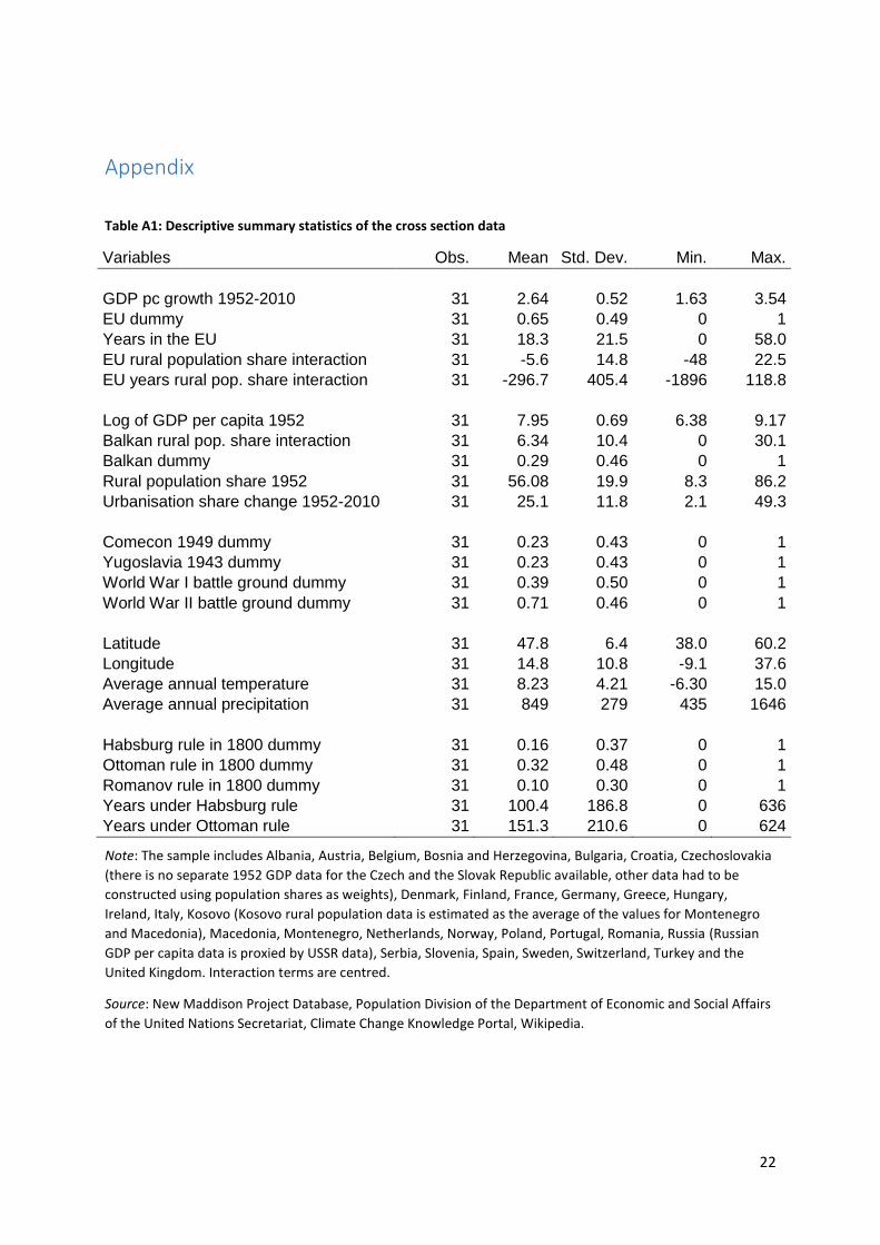
22
Appendix
Table A1: Descriptive summary statistics of the cross section data
Variables Obs. Mean Std. Dev. Min. Max.
GDP pc growth 1952-2010 31 2.64 0.52 1.63 3.54
EU dummy 31 0.65 0.49 0 1
Years in the EU 31 18.3 21.5 0 58.0
EU rural population share interaction 31 -5.6 14.8 -48 22.5
EU years rural pop. share interaction 31 -296.7 405.4 -1896 118.8
Log of GDP per capita 1952 31 7.95 0.69 6.38 9.17
Balkan rural pop. share interaction 31 6.34 10.4 0 30.1
Balkan dummy 31 0.29 0.46 0 1
Rural population share 1952 31 56.08 19.9 8.3 86.2
Urbanisation share change 1952-2010 31 25.1 11.8 2.1 49.3
Comecon 1949 dummy 31 0.23 0.43 0 1
Yugoslavia 1943 dummy 31 0.23 0.43 0 1
World War I battle ground dummy 31 0.39 0.50 0 1
World War II battle ground dummy 31 0.71 0.46 0 1
Latitude 31 47.8 6.4 38.0 60.2
Longitude 31 14.8 10.8 -9.1 37.6
Average annual temperature 31 8.23 4.21 -6.30 15.0
Average annual precipitation 31 849 279 435 1646
Habsburg rule in 1800 dummy 31 0.16 0.37 0 1
Ottoman rule in 1800 dummy 31 0.32 0.48 0 1
Romanov rule in 1800 dummy 31 0.10 0.30 0 1
Years under Habsburg rule 31 100.4 186.8 0 636
Years under Ottoman rule 31 151.3 210.6 0 624
Note: The sample includes Albania, Austria, Belgium, Bosnia and Herzegovina, Bulgaria, Croatia, Czechoslovakia
(there is no separate 1952 GDP data for the Czech and the Slovak Republic available, other data had to be
constructed using population shares as weights), Denmark, Finland, France, Germany, Greece, Hungary,
Ireland, Italy, Kosovo (Kosovo rural population data is estimated as the average of the values for Montenegro
and Macedonia), Macedonia, Montenegro, Netherlands, Norway, Poland, Portugal, Romania, Russia (Russian
GDP per capita data is proxied by USSR data), Serbia, Slovenia, Spain, Sweden, Switzerland, Turkey and the
United Kingdom. Interaction terms are centred.
Source: New Maddison Project Database, Population Division of the Department of Economic and Social Affairs
of the United Nations Secretariat, Climate Change Knowledge Portal, Wikipedia.
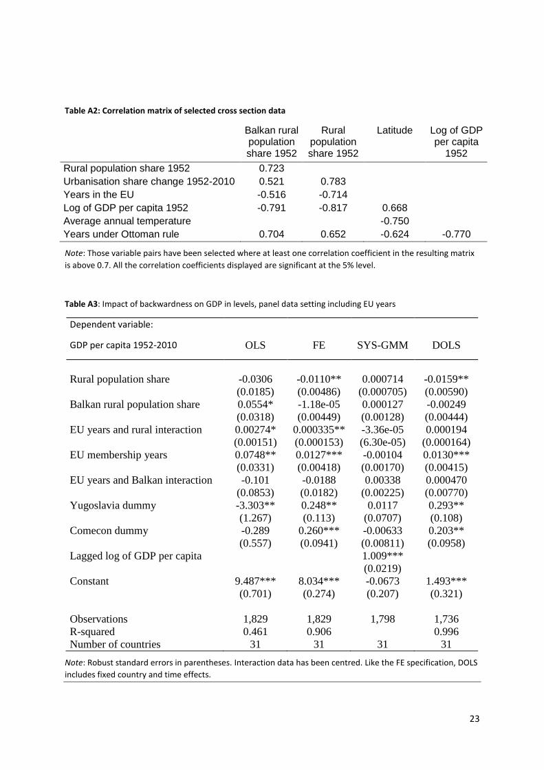
23
Table A2: Correlation matrix of selected cross section data
Balkan rural population share 1952
Rural population share 1952
Latitude Log of GDP per capita
1952
Rural population share 1952 0.723
Urbanisation share change 1952-2010 0.521 0.783
Years in the EU -0.516 -0.714
Log of GDP per capita 1952 -0.791 -0.817 0.668
Average annual temperature -0.750
Years under Ottoman rule 0.704 0.652 -0.624 -0.770
Note: Those variable pairs have been selected where at least one correlation coefficient in the resulting matrix
is above 0.7. All the correlation coefficients displayed are significant at the 5% level.
Table A3: Impact of backwardness on GDP in levels, panel data setting including EU years
Dependent variable:
GDP per capita 1952-2010 OLS FE SYS-GMM DOLS
Rural population share -0.0306 -0.0110** 0.000714 -0.0159**
(0.0185) (0.00486) (0.000705) (0.00590)
Balkan rural population share 0.0554* -1.18e-05 0.000127 -0.00249
(0.0318) (0.00449) (0.00128) (0.00444)
EU years and rural interaction 0.00274* 0.000335** -3.36e-05 0.000194
(0.00151) (0.000153) (6.30e-05) (0.000164)
EU membership years 0.0748** 0.0127*** -0.00104 0.0130***
(0.0331) (0.00418) (0.00170) (0.00415)
EU years and Balkan interaction -0.101 -0.0188 0.00338 0.000470
(0.0853) (0.0182) (0.00225) (0.00770)
Yugoslavia dummy -3.303** 0.248** 0.0117 0.293**
(1.267) (0.113) (0.0707) (0.108)
Comecon dummy -0.289 0.260*** -0.00633 0.203**
(0.557) (0.0941) (0.00811) (0.0958)
Lagged log of GDP per capita 1.009***
(0.0219)
Constant 9.487*** 8.034*** -0.0673 1.493***
(0.701) (0.274) (0.207) (0.321)
Observations 1,829 1,829 1,798 1,736
R-squared 0.461 0.906 0.996
Number of countries 31 31 31 31
Note: Robust standard errors in parentheses. Interaction data has been centred. Like the FE specification, DOLS
includes fixed country and time effects.
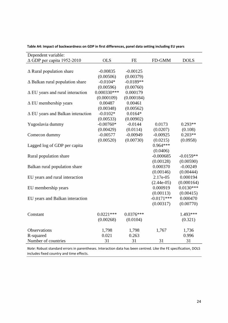
24
Table A4: Impact of backwardness on GDP in first differences, panel data setting including EU years
Dependent variable:
Δ GDP per capita 1952-2010 OLS FE FD-GMM DOLS
Δ Rural population share -0.00835 -0.00125
(0.00506) (0.00379)
Δ Balkan rural population share -0.0104* -0.0189**
(0.00596) (0.00760)
Δ EU years and rural interaction 0.000330*** 0.000179
(0.000109) (0.000184)
Δ EU membership years 0.00487 0.00461
(0.00348) (0.00562)
Δ EU years and Balkan interaction -0.0102* 0.0164*
(0.00533) (0.00902)
Yugoslavia dummy -0.00760* -0.0144 0.0173 0.293**
(0.00429) (0.0114) (0.0207) (0.108)
Comecon dummy -0.00577 -0.00949 -0.00925 0.203**
(0.00520) (0.00730) (0.0215) (0.0958)
Lagged log of GDP per capita 0.964***
(0.0406)
Rural population share -0.000685 -0.0159**
(0.00128) (0.00590)
Balkan rural population share 0.000370 -0.00249
(0.00146) (0.00444)
EU years and rural interaction 2.17e-05 0.000194
(2.44e-05) (0.000164)
EU membership years 0.000919 0.0130***
(0.00113) (0.00415)
EU years and Balkan interaction -0.0171*** 0.000470
(0.00317) (0.00770)
Constant 0.0221*** 0.0376*** 1.493***
(0.00268) (0.0104) (0.321)
Observations 1,798 1,798 1,767 1,736
R-squared 0.021 0.263 0.996
Number of countries 31 31 31 31
Note: Robust standard errors in parentheses. Interaction data has been centred. Like the FE specification, DOLS
includes fixed country and time effects.
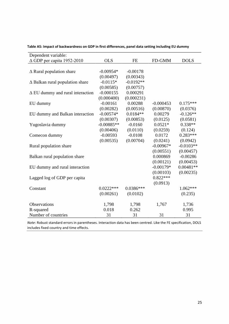
25
Table A5: Impact of backwardness on GDP in first differences, panel data setting including EU dummy
Dependent variable:
Δ GDP per capita 1952-2010 OLS FE FD-GMM DOLS
Δ Rural population share -0.00954* -0.00178
(0.00497) (0.00343)
Δ Balkan rural population share -0.0115* -0.0192**
(0.00585) (0.00757)
Δ EU dummy and rural interaction -0.000155 0.000291
(0.000400) (0.000231)
EU dummy -0.00161 0.00288 -0.000453 0.175***
(0.00282) (0.00516) (0.00870) (0.0376)
EU dummy and Balkan interaction -0.00574* 0.0184** 0.00279 -0.126**
(0.00307) (0.00853) (0.0125) (0.0581)
Yugoslavia dummy -0.00885** -0.0160 0.0521* 0.338**
(0.00406) (0.0110) (0.0259) (0.124)
Comecon dummy -0.00593 -0.0108 0.0172 0.283***
(0.00535) (0.00704) (0.0241) (0.0942)
Rural population share -0.00967* -0.0103**
(0.00551) (0.00457)
Balkan rural population share 0.000869 -0.00286
(0.00121) (0.00453)
EU dummy and rural interaction -0.00179* 0.00481**
(0.00103) (0.00235)
Lagged log of GDP per capita 0.822***
(0.0913)
Constant 0.0222*** 0.0386*** 1.062***
(0.00261) (0.0102) (0.235)
Observations 1,798 1,798 1,767 1,736
R-squared 0.018 0.262 0.995
Number of countries 31 31 31 31
Note: Robust standard errors in parentheses. Interaction data has been centred. Like the FE specification, DOLS
includes fixed country and time effects.
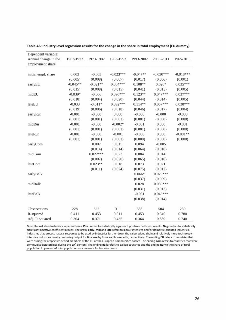
26
Table A6: Industry level regression results for the change in the share in total employment (EU dummy)
Dependent variable:
Annual change in the 1963-1972 1973-1982 1983-1992 1993-2002 2003-2011 1965-2011
employment share
initial empl. share 0.003 -0.003 -0.023*** -0.047** -0.030*** -0.018***
(0.005) (0.008) (0.007) (0.017) (0.006) (0.001)
earlyEU -0.045** -0.021** 0.084*** 0.108** 0.026* 0.035***
(0.015) (0.008) (0.015) (0.041) (0.015) (0.005)
midEU -0.039* -0.006 0.090*** 0.123** 0.047*** 0.037***
(0.018) (0.004) (0.020) (0.044) (0.014) (0.005)
lateEU -0.033 -0.011* 0.092*** 0.114** 0.057*** 0.038***
(0.019) (0.006) (0.018) (0.046) (0.017) (0.004)
earlyRur -0.001 -0.000 0.000 -0.000 -0.000 -0.000
(0.001) (0.001) (0.001) (0.001) (0.000) (0.000)
midRur -0.001 -0.000 -0.002* -0.001 0.000 -0.001
(0.001) (0.001) (0.001) (0.001) (0.000) (0.000)
lateRur -0.001 -0.000 -0.001 -0.000 0.000 -0.001**
(0.001) (0.001) (0.001) (0.000) (0.000) (0.000)
earlyCom 0.007 0.015 0.094 -0.005
(0.014) (0.014) (0.064) (0.010)
midCom 0.022*** 0.023 0.084 0.014
(0.007) (0.020) (0.065) (0.010)
lateCom 0.023** 0.018 0.073 0.021
(0.011) (0.024) (0.075) (0.012)
earlyBalk 0.066* 0.079***
(0.037) (0.009)
midBalk 0.028 0.059***
(0.031) (0.013)
lateBalk -0.031 0.045***
(0.038) (0.014)
Observations 228 322 311 388 504 230
R-squared 0.411 0.453 0.511 0.453 0.640 0.780
Adj. R-squared 0.304 0.371 0.435 0.364 0.589 0.740
Note: Robust standard errors in parentheses. Pos.: refers to statistically significant positive coefficient results. Neg.: refers to statistically significant negative coefficient results. The prefix early, mid and late refers to labour intensive and/or domestic-oriented industries, industries that process natural resources to be used by industries further down the value-added chain and relatively more technology-intensive industries mostly producing output for final use by firms and households, respectively. The ending EU refers to countries that were during the respective period members of the EU or the European Communities earlier. The ending Com refers to countries that were communist dictatorships during the 20th century. The ending Balk refers to Balkan countries and the ending Rur to the share of rural population in percent of total population as a measure for backwardness.
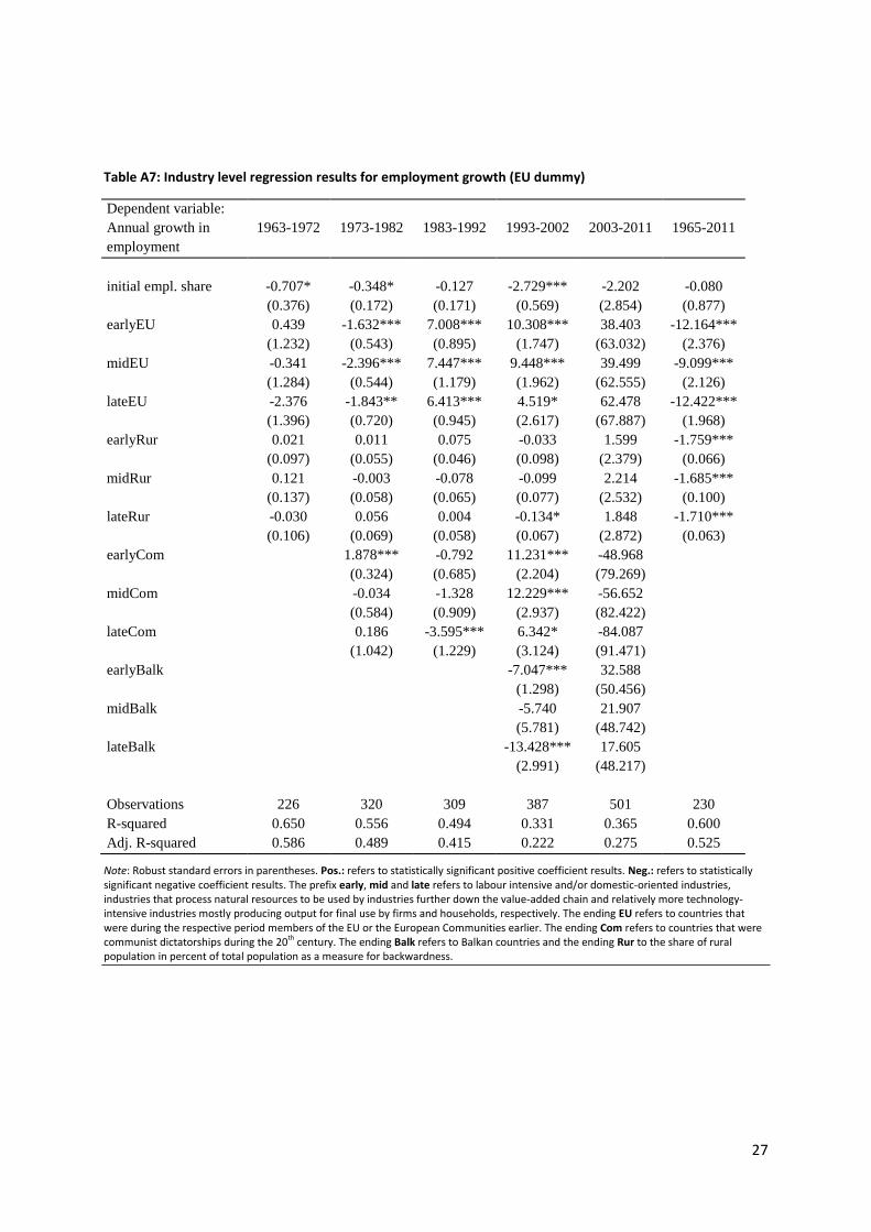
27
Table A7: Industry level regression results for employment growth (EU dummy)
Dependent variable:
Annual growth in 1963-1972 1973-1982 1983-1992 1993-2002 2003-2011 1965-2011
employment
initial empl. share -0.707* -0.348* -0.127 -2.729*** -2.202 -0.080
(0.376) (0.172) (0.171) (0.569) (2.854) (0.877)
earlyEU 0.439 -1.632*** 7.008*** 10.308*** 38.403 -12.164***
(1.232) (0.543) (0.895) (1.747) (63.032) (2.376)
midEU -0.341 -2.396*** 7.447*** 9.448*** 39.499 -9.099***
(1.284) (0.544) (1.179) (1.962) (62.555) (2.126)
lateEU -2.376 -1.843** 6.413*** 4.519* 62.478 -12.422***
(1.396) (0.720) (0.945) (2.617) (67.887) (1.968)
earlyRur 0.021 0.011 0.075 -0.033 1.599 -1.759***
(0.097) (0.055) (0.046) (0.098) (2.379) (0.066)
midRur 0.121 -0.003 -0.078 -0.099 2.214 -1.685***
(0.137) (0.058) (0.065) (0.077) (2.532) (0.100)
lateRur -0.030 0.056 0.004 -0.134* 1.848 -1.710***
(0.106) (0.069) (0.058) (0.067) (2.872) (0.063)
earlyCom 1.878*** -0.792 11.231*** -48.968
(0.324) (0.685) (2.204) (79.269)
midCom -0.034 -1.328 12.229*** -56.652
(0.584) (0.909) (2.937) (82.422)
lateCom 0.186 -3.595*** 6.342* -84.087
(1.042) (1.229) (3.124) (91.471)
earlyBalk -7.047*** 32.588
(1.298) (50.456)
midBalk -5.740 21.907
(5.781) (48.742)
lateBalk -13.428*** 17.605
(2.991) (48.217)
Observations 226 320 309 387 501 230
R-squared 0.650 0.556 0.494 0.331 0.365 0.600
Adj. R-squared 0.586 0.489 0.415 0.222 0.275 0.525
Note: Robust standard errors in parentheses. Pos.: refers to statistically significant positive coefficient results. Neg.: refers to statistically significant negative coefficient results. The prefix early, mid and late refers to labour intensive and/or domestic-oriented industries, industries that process natural resources to be used by industries further down the value-added chain and relatively more technology-intensive industries mostly producing output for final use by firms and households, respectively. The ending EU refers to countries that were during the respective period members of the EU or the European Communities earlier. The ending Com refers to countries that were communist dictatorships during the 20th century. The ending Balk refers to Balkan countries and the ending Rur to the share of rural population in percent of total population as a measure for backwardness.
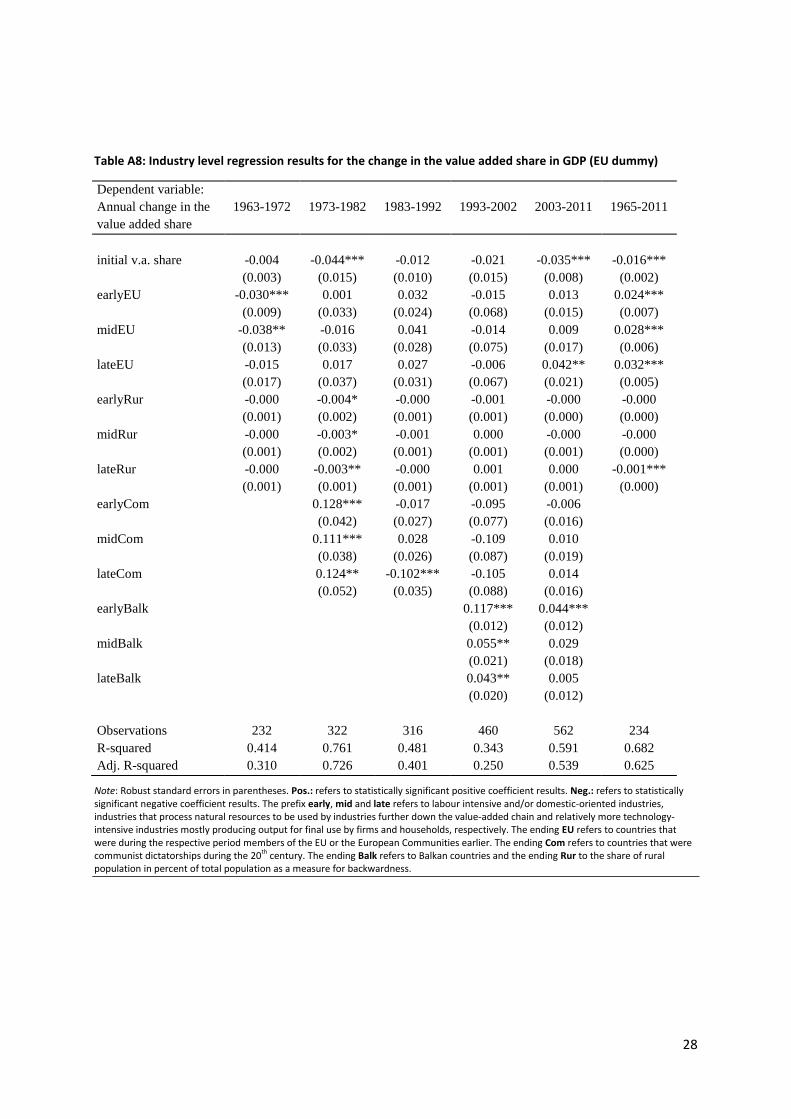
28
Table A8: Industry level regression results for the change in the value added share in GDP (EU dummy)
Dependent variable:
Annual change in the 1963-1972 1973-1982 1983-1992 1993-2002 2003-2011 1965-2011
value added share
initial v.a. share -0.004 -0.044*** -0.012 -0.021 -0.035*** -0.016***
(0.003) (0.015) (0.010) (0.015) (0.008) (0.002)
earlyEU -0.030*** 0.001 0.032 -0.015 0.013 0.024***
(0.009) (0.033) (0.024) (0.068) (0.015) (0.007)
midEU -0.038** -0.016 0.041 -0.014 0.009 0.028***
(0.013) (0.033) (0.028) (0.075) (0.017) (0.006)
lateEU -0.015 0.017 0.027 -0.006 0.042** 0.032***
(0.017) (0.037) (0.031) (0.067) (0.021) (0.005)
earlyRur -0.000 -0.004* -0.000 -0.001 -0.000 -0.000
(0.001) (0.002) (0.001) (0.001) (0.000) (0.000)
midRur -0.000 -0.003* -0.001 0.000 -0.000 -0.000
(0.001) (0.002) (0.001) (0.001) (0.001) (0.000)
lateRur -0.000 -0.003** -0.000 0.001 0.000 -0.001***
(0.001) (0.001) (0.001) (0.001) (0.001) (0.000)
earlyCom 0.128*** -0.017 -0.095 -0.006
(0.042) (0.027) (0.077) (0.016)
midCom 0.111*** 0.028 -0.109 0.010
(0.038) (0.026) (0.087) (0.019)
lateCom 0.124** -0.102*** -0.105 0.014
(0.052) (0.035) (0.088) (0.016)
earlyBalk 0.117*** 0.044***
(0.012) (0.012)
midBalk 0.055** 0.029
(0.021) (0.018)
lateBalk 0.043** 0.005
(0.020) (0.012)
Observations 232 322 316 460 562 234
R-squared 0.414 0.761 0.481 0.343 0.591 0.682
Adj. R-squared 0.310 0.726 0.401 0.250 0.539 0.625
Note: Robust standard errors in parentheses. Pos.: refers to statistically significant positive coefficient results. Neg.: refers to statistically significant negative coefficient results. The prefix early, mid and late refers to labour intensive and/or domestic-oriented industries, industries that process natural resources to be used by industries further down the value-added chain and relatively more technology-intensive industries mostly producing output for final use by firms and households, respectively. The ending EU refers to countries that were during the respective period members of the EU or the European Communities earlier. The ending Com refers to countries that were communist dictatorships during the 20th century. The ending Balk refers to Balkan countries and the ending Rur to the share of rural population in percent of total population as a measure for backwardness.

29
Table A9: Industry level regression results for growth of value added (EU dummy)
Dependent variable:
Annual growth in 1963-1972 1973-1982 1983-1992 1993-2002 2003-2011 1965-2011
value added
initial v.a. share -0.245 0.633 0.049 -4.449 -3.702* -1.085**
(0.431) (1.363) (0.470) (3.235) (1.931) (0.386)
earlyEU 0.899 3.982 7.456*** 16.129* 108.202 5.234***
(2.325) (4.854) (1.804) (9.363) (101.383) (1.613)
midEU -1.383 1.355 4.667 29.304 112.492 7.932***
(2.215) (4.392) (3.083) (17.552) (103.956) (1.605)
lateEU -1.087 2.156 4.665** 22.718 131.383 6.383***
(2.358) (3.872) (1.838) (14.617) (109.045) (1.277)
earlyRur -0.076 0.179 -0.048 -0.133 3.784 -0.311***
(0.132) (0.151) (0.116) (0.406) (3.954) (0.088)
midRur -0.023 0.212 -0.140 -0.372 4.404 -0.383***
(0.129) (0.184) (0.119) (0.935) (4.148) (0.123)
lateRur -0.094 0.186 -0.125 0.456 4.591 -0.314***
(0.122) (0.141) (0.122) (0.443) (4.659) (0.100)
earlyCom 20.894*** 5.751** 3.522 -133.078
(6.897) (2.633) (13.170) (130.655)
midCom 9.307* 4.307 45.437 -146.176
(4.578) (5.019) (41.228) (136.425)
lateCom 7.259 -4.378* 10.188 -172.698
(6.345) (2.383) (15.246) (150.766)
earlyBalk 19.034*** 82.518
(6.219) (81.405)
midBalk -5.182 86.929
(21.701) (79.777)
lateBalk -7.480 71.612
(9.492) (77.250)
Observations 230 318 309 415 525 234
R-squared 0.743 0.244 0.444 0.197 0.343 0.667
Adj. R-squared 0.697 0.129 0.356 0.075 0.253 0.607
Note: Robust standard errors in parentheses. Pos.: refers to statistically significant positive coefficient results. Neg.: refers to statistically significant negative coefficient results. The prefix early, mid and late refers to labour intensive and/or domestic-oriented industries, industries that process natural resources to be used by industries further down the value-added chain and relatively more technology-intensive industries mostly producing output for final use by firms and households, respectively. The ending EU refers to countries that were during the respective period members of the EU or the European Communities earlier. The ending Com refers to countries that were communist dictatorships during the 20th century. The ending Balk refers to Balkan countries and the ending Rur to the share of rural population in percent of total population as a measure for backwardness.
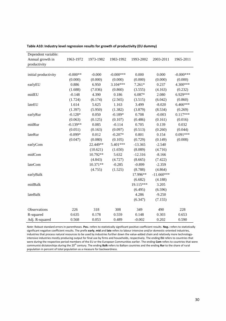
30
Table A10: Industry level regression results for growth of productivity (EU dummy)
Dependent variable:
Annual growth in 1963-1972 1973-1982 1983-1992 1993-2002 2003-2011 1965-2011
productivity
initial productivity -0.000** -0.000 -0.000*** 0.000 0.000 -0.000***
(0.000) (0.000) (0.000) (0.000) (0.000) (0.000)
earlyEU 0.886 6.950 3.104*** 7.261* 0.237 4.300***
(1.688) (7.036) (0.860) (3.555) (4.163) (0.232)
midEU -0.148 4.390 0.186 6.087* 2.080 6.929***
(1.724) (6.174) (2.565) (3.515) (6.042) (0.860)
lateEU 1.614 5.625 1.163 3.499 -8.020 6.466***
(1.397) (5.950) (1.382) (3.879) (8.534) (0.269)
earlyRur -0.128* 0.050 -0.189* 0.708 -0.003 0.117***
(0.063) (0.125) (0.107) (0.486) (0.161) (0.016)
midRur -0.139** 0.085 -0.114 0.705 0.139 0.032
(0.051) (0.163) (0.097) (0.513) (0.260) (0.044)
lateRur -0.099* 0.012 -0.207* 0.801 0.154 0.091***
(0.047) (0.080) (0.105) (0.729) (0.149) (0.008)
earlyCom 22.449** 5.401*** -13.365 -2.540
(10.621) (1.650) (8.089) (4.716)
midCom 10.792** 5.632 -12.316 -8.166
(4.843) (4.727) (8.665) (7.422)
lateCom 10.371** -0.285 -0.899 -2.359
(4.755) (1.525) (8.788) (4.864)
earlyBalk 17.996** -11.660***
(6.682) (4.188)
midBalk 19.115*** 3.205
(6.495) (6.596)
lateBalk 4.286 -9.250
(6.347) (7.155)
Observations 226 318 308 349 490 228
R-squared 0.635 0.178 0.559 0.148 0.303 0.653
Adj. R-squared 0.568 0.053 0.489 -0.002 0.202 0.590
Note: Robust standard errors in parentheses. Pos.: refers to statistically significant positive coefficient results. Neg.: refers to statistically significant negative coefficient results. The prefix early, mid and late refers to labour intensive and/or domestic-oriented industries, industries that process natural resources to be used by industries further down the value-added chain and relatively more technology-intensive industries mostly producing output for final use by firms and households, respectively. The ending EU refers to countries that were during the respective period members of the EU or the European Communities earlier. The ending Com refers to countries that were communist dictatorships during the 20th century. The ending Balk refers to Balkan countries and the ending Rur to the share of rural population in percent of total population as a measure for backwardness.
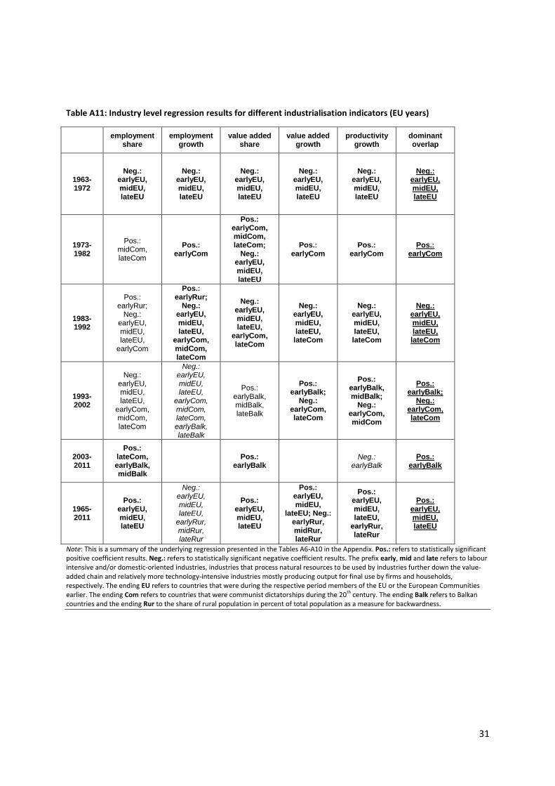
31
Table A11: Industry level regression results for different industrialisation indicators (EU years)
employment
share employment
growth value added
share value added
growth productivity
growth dominant overlap
1963-1972
Neg.: earlyEU, midEU, lateEU
Neg.: earlyEU, midEU, lateEU
Neg.: earlyEU, midEU, lateEU
Neg.: earlyEU, midEU, lateEU
Neg.: earlyEU, midEU, lateEU
Neg.: earlyEU, midEU, lateEU
1973-1982
Pos.: midCom, lateCom
Pos.: earlyCom
Pos.: earlyCom, midCom, lateCom;
Neg.: earlyEU, midEU, lateEU
Pos.: earlyCom
Pos.: earlyCom
Pos.: earlyCom
1983-1992
Pos.: earlyRur;
Neg.: earlyEU, midEU, lateEU,
earlyCom
Pos.: earlyRur;
Neg.: earlyEU, midEU, lateEU,
earlyCom, midCom, lateCom
Neg.: earlyEU, midEU, lateEU,
earlyCom, lateCom
Neg.: earlyEU, midEU, lateEU, lateCom
Neg.: earlyEU, midEU, lateEU, lateCom
Neg.: earlyEU, midEU, lateEU, lateCom
1993-2002
Neg.: earlyEU, midEU, lateEU,
earlyCom, midCom, lateCom
Neg.: earlyEU, midEU, lateEU,
earlyCom, midCom, lateCom, earlyBalk, lateBalk
Pos.: earlyBalk, midBalk, lateBalk
Pos.: earlyBalk;
Neg.: earlyCom, lateCom
Pos.: earlyBalk, midBalk;
Neg.: earlyCom, midCom
Pos.: earlyBalk;
Neg.: earlyCom, lateCom
2003-2011
Pos.: lateCom, earlyBalk, midBalk
Pos.:
earlyBalk
Neg.: earlyBalk
Pos.: earlyBalk
1965-2011
Pos.: earlyEU, midEU, lateEU
Neg.: earlyEU, midEU, lateEU,
earlyRur, midRur, lateRur
Pos.: earlyEU, midEU, lateEU
Pos.: earlyEU, midEU,
lateEU; Neg.: earlyRur, midRur, lateRur
Pos.: earlyEU, midEU, lateEU,
earlyRur, lateRur
Pos.: earlyEU, midEU, lateEU
Note: This is a summary of the underlying regression presented in the Tables A6-A10 in the Appendix. Pos.: refers to statistically significant positive coefficient results. Neg.: refers to statistically significant negative coefficient results. The prefix early, mid and late refers to labour intensive and/or domestic-oriented industries, industries that process natural resources to be used by industries further down the value-added chain and relatively more technology-intensive industries mostly producing output for final use by firms and households, respectively. The ending EU refers to countries that were during the respective period members of the EU or the European Communities earlier. The ending Com refers to countries that were communist dictatorships during the 20th century. The ending Balk refers to Balkan countries and the ending Rur to the share of rural population in percent of total population as a measure for backwardness.
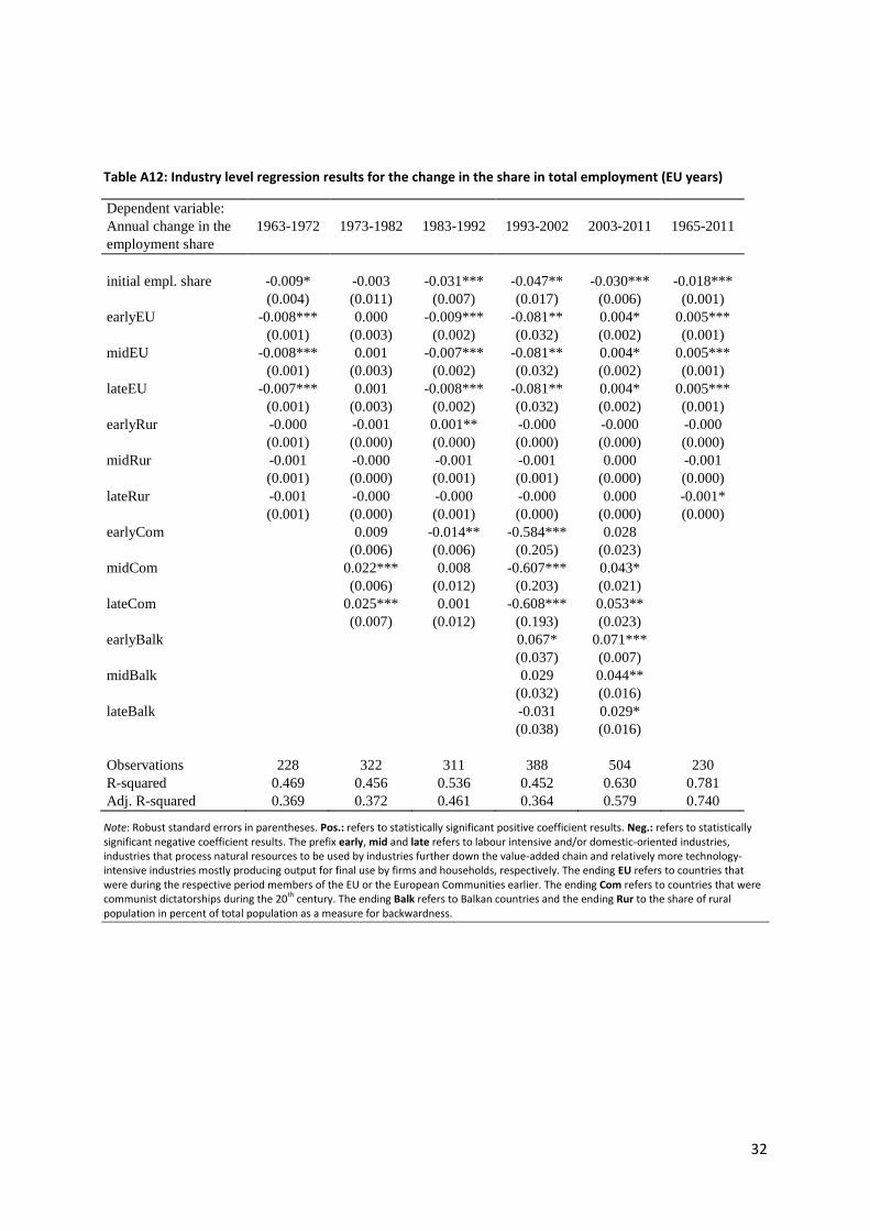
32
Table A12: Industry level regression results for the change in the share in total employment (EU years)
Dependent variable:
Annual change in the 1963-1972 1973-1982 1983-1992 1993-2002 2003-2011 1965-2011
employment share
initial empl. share -0.009* -0.003 -0.031*** -0.047** -0.030*** -0.018***
(0.004) (0.011) (0.007) (0.017) (0.006) (0.001)
earlyEU -0.008*** 0.000 -0.009*** -0.081** 0.004* 0.005***
(0.001) (0.003) (0.002) (0.032) (0.002) (0.001)
midEU -0.008*** 0.001 -0.007*** -0.081** 0.004* 0.005***
(0.001) (0.003) (0.002) (0.032) (0.002) (0.001)
lateEU -0.007*** 0.001 -0.008*** -0.081** 0.004* 0.005***
(0.001) (0.003) (0.002) (0.032) (0.002) (0.001)
earlyRur -0.000 -0.001 0.001** -0.000 -0.000 -0.000
(0.001) (0.000) (0.000) (0.000) (0.000) (0.000)
midRur -0.001 -0.000 -0.001 -0.001 0.000 -0.001
(0.001) (0.000) (0.001) (0.001) (0.000) (0.000)
lateRur -0.001 -0.000 -0.000 -0.000 0.000 -0.001*
(0.001) (0.000) (0.001) (0.000) (0.000) (0.000)
earlyCom 0.009 -0.014** -0.584*** 0.028
(0.006) (0.006) (0.205) (0.023)
midCom 0.022*** 0.008 -0.607*** 0.043*
(0.006) (0.012) (0.203) (0.021)
lateCom 0.025*** 0.001 -0.608*** 0.053**
(0.007) (0.012) (0.193) (0.023)
earlyBalk 0.067* 0.071***
(0.037) (0.007)
midBalk 0.029 0.044**
(0.032) (0.016)
lateBalk -0.031 0.029*
(0.038) (0.016)
Observations 228 322 311 388 504 230
R-squared 0.469 0.456 0.536 0.452 0.630 0.781
Adj. R-squared 0.369 0.372 0.461 0.364 0.579 0.740
Note: Robust standard errors in parentheses. Pos.: refers to statistically significant positive coefficient results. Neg.: refers to statistically significant negative coefficient results. The prefix early, mid and late refers to labour intensive and/or domestic-oriented industries, industries that process natural resources to be used by industries further down the value-added chain and relatively more technology-intensive industries mostly producing output for final use by firms and households, respectively. The ending EU refers to countries that were during the respective period members of the EU or the European Communities earlier. The ending Com refers to countries that were communist dictatorships during the 20th century. The ending Balk refers to Balkan countries and the ending Rur to the share of rural population in percent of total population as a measure for backwardness.
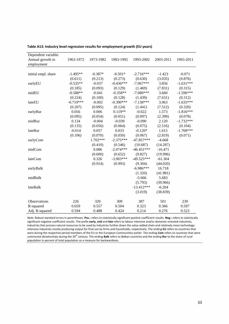
33
Table A13: Industry level regression results for employment growth (EU years)
Dependent variable:
Annual growth in 1963-1972 1973-1982 1983-1992 1993-2002 2003-2011 1965-2011
employment
initial empl. share -1.495** -0.387* -0.501* -2.716*** -1.423 -0.071
(0.611) (0.213) (0.273) (0.630) (3.035) (0.876)
earlyEU -0.535** -0.037 -0.436*** -7.067*** 3.856 -1.631***
(0.185) (0.093) (0.129) (1.469) (7.831) (0.315)
midEU -0.588** -0.041 -0.358** -7.080*** 3.660 -1.596***
(0.224) (0.100) (0.128) (1.439) (7.631) (0.312)
lateEU -0.719*** -0.002 -0.390*** -7.138*** 3.063 -1.635***
(0.207) (0.095) (0.124) (1.441) (7.512) (0.320)
earlyRur 0.056 0.006 0.119** -0.022 1.573 -1.816***
(0.095) (0.054) (0.051) (0.097) (2.399) (0.078)
midRur 0.134 -0.004 -0.039 -0.090 2.120 -1.732***
(0.135) (0.056) (0.064) (0.075) (2.516) (0.104)
lateRur -0.014 0.057 0.033 -0.120* 1.615 -1.768***
(0.106) (0.070) (0.050) (0.067) (2.819) (0.071)
earlyCom 1.702*** -2.375*** -47.857*** -4.668
(0.410) (0.546) (10.687) (14.287)
midCom 0.086 -2.074*** -46.451*** -16.471
(0.600) (0.652) (9.827) (19.996)
lateCom 0.326 -3.903*** -49.525*** -61.304
(0.914) (0.993) (9.304) (44.020)
earlyBalk -6.986*** 16.718
(1.320) (41.981)
midBalk -5.666 5.683
(5.793) (39.966)
lateBalk -13.412*** -6.204
(3.019) (38.839)
Observations 226 320 309 387 501 230
R-squared 0.659 0.557 0.504 0.323 0.366 0.597
Adj. R-squared 0.594 0.488 0.424 0.214 0.276 0.523
Note: Robust standard errors in parentheses. Pos.: refers to statistically significant positive coefficient results. Neg.: refers to statistically significant negative coefficient results. The prefix early, mid and late refers to labour intensive and/or domestic-oriented industries, industries that process natural resources to be used by industries further down the value-added chain and relatively more technology-intensive industries mostly producing output for final use by firms and households, respectively. The ending EU refers to countries that were during the respective period members of the EU or the European Communities earlier. The ending Com refers to countries that were communist dictatorships during the 20th century. The ending Balk refers to Balkan countries and the ending Rur to the share of rural population in percent of total population as a measure for backwardness.

34
Table A14: Industry level regression results for the change in the value added share in GDP (EU years)
Dependent variable:
Annual change in the 1963-1972 1973-1982 1983-1992 1993-2002 2003-2011 1965-2011
value added share
initial v.a. share -0.011** -0.055*** -0.021 -0.021 -0.035*** -0.017***
(0.005) (0.016) (0.013) (0.015) (0.008) (0.002)
earlyEU -0.006** -0.017** -0.010** 0.012 0.002 0.004***
(0.002) (0.006) (0.004) (0.050) (0.002) (0.001)
midEU -0.006** -0.017** -0.009** 0.012 0.002 0.003***
(0.002) (0.006) (0.004) (0.050) (0.002) (0.001)
lateEU -0.005** -0.016** -0.010** 0.012 0.003 0.004***
(0.002) (0.006) (0.004) (0.050) (0.002) (0.001)
earlyRur 0.000 -0.002 0.001 -0.001 -0.000 -0.000
(0.001) (0.001) (0.001) (0.001) (0.000) (0.000)
midRur -0.000 -0.002 -0.000 0.000 0.000 -0.000
(0.001) (0.001) (0.001) (0.001) (0.000) (0.000)
lateRur -0.000 -0.002* 0.001 0.001 0.000 -0.000
(0.001) (0.001) (0.001) (0.001) (0.001) (0.000)
earlyCom 0.075*** -0.040** 0.009 0.010
(0.016) (0.016) (0.346) (0.022)
midCom 0.078*** 0.015 -0.018 0.021
(0.016) (0.013) (0.340) (0.022)
lateCom 0.098*** -0.109*** -0.012 0.034
(0.029) (0.024) (0.336) (0.023)
earlyBalk 0.117*** 0.042***
(0.012) (0.010)
midBalk 0.055** 0.028*
(0.021) (0.016)
lateBalk 0.043** -0.003
(0.020) (0.013)
Observations 232 322 316 460 562 234
R-squared 0.439 0.785 0.501 0.344 0.585 0.686
Adj. R-squared 0.336 0.752 0.422 0.251 0.533 0.629
Note: Robust standard errors in parentheses. Pos.: refers to statistically significant positive coefficient results. Neg.: refers to statistically significant negative coefficient results. The prefix early, mid and late refers to labour intensive and/or domestic-oriented industries, industries that process natural resources to be used by industries further down the value-added chain and relatively more technology-intensive industries mostly producing output for final use by firms and households, respectively. The ending EU refers to countries that were during the respective period members of the EU or the European Communities earlier. The ending Com refers to countries that were communist dictatorships during the 20th century. The ending Balk refers to Balkan countries and the ending Rur to the share of rural population in percent of total population as a measure for backwardness.

35
Table A15: Industry level regression results for growth of value added (EU years)
Dependent variable:
Annual growth in 1963-1972 1973-1982 1983-1992 1993-2002 2003-2011 1965-2011
value added
initial v.a. share -1.913** -0.478 -1.354* -4.394 -2.716 -1.174**
(0.631) (0.602) (0.648) (3.138) (1.807) (0.385)
earlyEU -1.374*** -1.663 -1.580*** -13.788* 12.531 0.744***
(0.231) (1.376) (0.261) (6.990) (12.382) (0.221)
midEU -1.504*** -1.703 -1.569*** -13.643* 12.310 0.697***
(0.236) (1.396) (0.273) (6.976) (12.144) (0.225)
lateEU -1.470*** -1.702 -1.558*** -13.542* 11.499 0.730***
(0.236) (1.414) (0.250) (6.952) (11.698) (0.233)
earlyRur 0.007 0.379 0.118 -0.157 3.722 -0.272**
(0.131) (0.280) (0.079) (0.428) (3.959) (0.098)
midRur 0.020 0.355 -0.047 -0.378 4.269 -0.371***
(0.125) (0.250) (0.095) (0.951) (4.092) (0.116)
lateRur -0.055 0.305 -0.033 0.437 4.216 -0.284**
(0.123) (0.199) (0.100) (0.421) (4.512) (0.106)
earlyCom 15.552*** 1.705 -111.730** -6.956
(3.992) (2.092) (48.041) (14.320)
midCom 5.964 3.092 -77.304* -24.905
(4.846) (3.062) (39.245) (26.981)
lateCom 5.029 -4.791*** -105.081** -74.381
(6.318) (1.538) (49.672) (54.566)
earlyBalk 19.041*** 57.063
(6.213) (64.827)
midBalk -5.182 60.071
(21.725) (62.020)
lateBalk -7.451 38.327
(9.466) (57.634)
Observations 230 318 309 415 525 234
R-squared 0.762 0.260 0.475 0.197 0.345 0.667
Adj. R-squared 0.717 0.145 0.390 0.074 0.256 0.607
Note: Robust standard errors in parentheses. Pos.: refers to statistically significant positive coefficient results. Neg.: refers to statistically significant negative coefficient results. The prefix early, mid and late refers to labour intensive and/or domestic-oriented industries, industries that process natural resources to be used by industries further down the value-added chain and relatively more technology-intensive industries mostly producing output for final use by firms and households, respectively. The ending EU refers to countries that were during the respective period members of the EU or the European Communities earlier. The ending Com refers to countries that were communist dictatorships during the 20th century. The ending Balk refers to Balkan countries and the ending Rur to the share of rural population in percent of total population as a measure for backwardness.
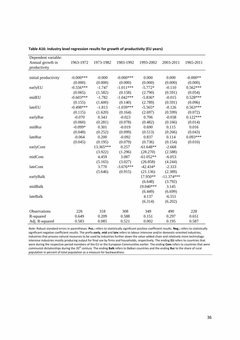
36
Table A16: Industry level regression results for growth of productivity (EU years)
Dependent variable:
Annual growth in 1963-1972 1973-1982 1983-1992 1993-2002 2003-2011 1965-2011
productivity
initial productivity -0.000*** -0.000 -0.000*** 0.000 0.000 -0.000**
(0.000) (0.000) (0.000) (0.000) (0.000) (0.000)
earlyEU -0.556*** -1.747 -1.011*** -5.772* -0.110 0.562***
(0.065) (1.582) (0.158) (2.790) (0.591) (0.054)
midEU -0.603*** -1.782 -1.042*** -5.836* -0.015 0.528***
(0.155) (1.600) (0.140) (2.789) (0.591) (0.096)
lateEU -0.498*** -1.813 -1.039*** -5.565* -0.126 0.563***
(0.115) (1.620) (0.164) (2.697) (0.599) (0.072)
earlyRur -0.070 0.343 -0.023 0.706 -0.038 0.122***
(0.060) (0.281) (0.078) (0.482) (0.166) (0.014)
midRur -0.099* 0.301 -0.019 0.690 0.115 0.016
(0.048) (0.252) (0.099) (0.513) (0.266) (0.043)
lateRur -0.064 0.200 -0.092 0.837 0.114 0.093***
(0.045) (0.195) (0.079) (0.736) (0.154) (0.010)
earlyCom 13.365*** 0.257 -61.648** -2.668
(3.922) (1.296) (28.270) (2.588)
midCom 4.459 3.087 -61.052** -6.053
(5.165) (3.027) (26.858) (4.244)
lateCom 3.770 -3.676*** -42.434* -2.333
(5.646) (0.915) (21.136) (2.389)
earlyBalk 17.950** -11.374***
(6.648) (3.792)
midBalk 19.040*** 3.145
(6.449) (6.699)
lateBalk 4.137 -6.551
(6.314) (6.202)
Observations 226 318 308 349 490 228
R-squared 0.649 0.209 0.588 0.151 0.297 0.651
Adj. R-squared 0.583 0.085 0.521 0.002 0.195 0.587
Note: Robust standard errors in parentheses. Pos.: refers to statistically significant positive coefficient results. Neg.: refers to statistically significant negative coefficient results. The prefix early, mid and late refers to labour intensive and/or domestic-oriented industries, industries that process natural resources to be used by industries further down the value-added chain and relatively more technology-intensive industries mostly producing output for final use by firms and households, respectively. The ending EU refers to countries that were during the respective period members of the EU or the European Communities earlier. The ending Com refers to countries that were communist dictatorships during the 20th century. The ending Balk refers to Balkan countries and the ending Rur to the share of rural population in percent of total population as a measure for backwardness.