The Wider Beneﬁts of Adult Learning: Work-Related Training

SOEPpaperson Multidisciplinary Panel Data Research

The GermanSocio-EconomicPanel study

The Wider Benefits of Adult Learning: Work-Related Training and Social Capital

Jens Ruhose, Stephan L. Thomsen, Insa Weilage

1004 201

8SOEP — The German Socio-Economic Panel Study at DIW Berlin 1004-2018

SOEPpapers on Multidisciplinary Panel Data Research at DIW Berlin This series presents research findings based either directly on data from the German Socio-Economic Panel study (SOEP) or using SOEP data as part of an internationally comparable data set (e.g. CNEF, ECHP, LIS, LWS, CHER/PACO). SOEP is a truly multidisciplinary household panel study covering a wide range of social and behavioral sciences: economics, sociology, psychology, survey methodology, econometrics and applied statistics, educational science, political science, public health, behavioral genetics, demography, geography, and sport science. The decision to publish a submission in SOEPpapers is made by a board of editors chosen by the DIW Berlin to represent the wide range of disciplines covered by SOEP. There is no external referee process and papers are either accepted or rejected without revision. Papers appear in this series as works in progress and may also appear elsewhere. They often represent preliminary studies and are circulated to encourage discussion. Citation of such a paper should account for its provisional character. A revised version may be requested from the author directly. Any opinions expressed in this series are those of the author(s) and not those of DIW Berlin. Research disseminated by DIW Berlin may include views on public policy issues, but the institute itself takes no institutional policy positions. The SOEPpapers are available at http://www.diw.de/soeppapers Editors: Jan Goebel (Spatial Economics) Stefan Liebig (Sociology) David Richter (Psychology) Carsten Schröder (Public Economics) Jürgen Schupp (Sociology) Conchita D’Ambrosio (Public Economics, DIW Research Fellow) Denis Gerstorf (Psychology, DIW Research Fellow) Elke Holst (Gender Studies, DIW Research Director) Martin Kroh (Political Science, Survey Methodology) Jörg-Peter Schräpler (Survey Methodology, DIW Research Fellow) Thomas Siedler (Empirical Economics, DIW Research Fellow) C. Katharina Spieß (Education and Family Economics) Gert G. Wagner (Social Sciences)

ISSN: 1864-6689 (online)

German Socio-Economic Panel (SOEP) DIW Berlin Mohrenstrasse 58 10117 Berlin, Germany Contact: [email protected]

The Wider Benefits of Adult Learning:Work-Related Training and Social Capital∗

Jens Ruhose† Stephan L. Thomsen‡ Insa Weilage§

December 3, 2018

Abstract

We propose a regression-adjusted matched difference-in-differences framework toestimate non-pecuniary returns to adult education. This approach combines kernelmatching with entropy balancing to account for selection bias and sorting on gains. Usingdata from the German SOEP, we evaluate the effect of work-related training, whichrepresents the largest portion of adult education in OECD countries, on individual socialcapital. Training increases participation in civic, political, and cultural activities whilenot crowding out social participation. Results are robust against a variety of potentiallyconfounding explanations. These findings imply positive externalities from work-relatedtraining over and above the well-documented labor market effects.JEL Codes: J24, I21, M53Keywords: non-pecuniary returns, social capital, work-related training, matcheddifference-in-differences approach, entropy balancing

∗Previous versions of this paper have been circulated under the title “Wider Benefits from ContinuousWork-Related Training". We are grateful to Guido Heineck, Sandra McNally, Jens Mohrenweiser, Ina Rüber,Josef Schrader, Nicole Tieben, Simon Wiederhold, Ludger Woessmann, Oleksandr Zhylyevskyy, and seminarand conference participants at the annual meetings of the EEA (Cologne), MEA/SOLE (Evanston), Verein fürSocialpolitik (Vienna), standing field committee on the economics of education of the Verein für Socialpolitik(Bern), the conference of the Centre for Vocational Education Research (London), Society for EmpiricalEducational Research (Basel), the IZA research seminar (Bonn), Goethe University Frankfurt, Leibniz UniversitätHannover, and Leuphana Universität Lüneburg for their most helpful comments and discussions. Financial supportby the German Federal Ministry of Education and Research (BMBF) through the project “Nicht-monetäre Erträgeder Weiterbildung: zivilgesellschaftliche Partizipation (NEWz)" is gratefully acknowledged.

†Leibniz Universität Hannover, Königsworther Platz 1, 30167 Hannover, CESifo, and IZA; E-mail:[email protected]

‡Leibniz Universität Hannover, Königsworther Platz 1, 30167 Hannover, ZEW, and IZA; E-mail:[email protected]

§Leibniz Universität Hannover, Königsworther Platz 1, 30167 Hannover; E-mail: [email protected]

1 Introduction

Updating skills and abilities over the life cycle is crucial for workers, firms, and entireeconomies seeking to prevent human capital depreciation and to remain competitive ina globalized and ever-changing work environment (OECD, 2005, 2013). Particularlyin industrialized countries, participation in continuing education and training (CET) hasbecome widespread. For example, according to the Survey of Adult Skills (PIAAC) 2015,approximately half of adults aged between 25 and 64 years took part in some CET activity(including open or distance-learning courses, private lessons, organized sessions for on-the-jobtraining, and workshops or seminars—some of which might be of short duration) in OECDcountries in a given year (OECD, 2017, p. 327). The majority of these activities arenonformal (approximately 92%), meaning that they are organized but are less institutionalizedand structured than formal learning activities (which usually lead to the granting of credentialsand certificates).1

While there are numerous studies showing that work-related training affects individual labormarket outcomes and benefits the performance of the firm, there is rarely any causal evidenceon the extent of further non-pecuniary benefits from CET (Field, 2011).2 Focusing on the caseof Germany, where participation rates are close to the OECD average,3 this paper makes twokey contributions to the literature on adult education. First, we address empirical challenges inthe evaluation of wider benefits from training by introducing a flexible econometric frameworkinto the literature, a framework that can be implemented with panel data. Second, we apply thisframework to identify the effects of work-related training, which constitutes the majority (82%)of nonformal CET in Germany and elsewhere (Federal Ministry of Education and Research,2015, 2017),4 on measures of civic/political, cultural, and social participation—measures thatare related to social capital at the individual level (Putnam, 1993). Social capital outcomesare high on the political agenda because social capital is considered to facilitate collaborationand cooperation within a society, yielding positive economic externalities (see Section 2 for adiscussion).

We use rich longitudinal panel data from the German Socio-Economic Panel Study (SOEP)from 1992 to 2014. These data offer detailed information on pecuniary and non-pecuniary

1The PIAAC survey shows that 39% of adults participate in non-formal education only, 4% participate informal education only, 7% participate in both formal and nonformal education, and 50% do not participate inCET. Formal education is defined as “planned education provided in the system of schools, colleges, universitiesand other formal educational institutions" (OECD, 2017, p. 325) and nonformal learning activities are “sustainededucational activity that does not correspond exactly to the definition of formal education."

2For example, Bassanini et al. (2007) and Leuven (2005) provide overview studies on individual labor marketoutcomes, and Acemoglu and Pischke (1998), Acemoglu and Pischke (1999), De Grip and Sauermann (2012,2013), and Loewenstein and Spletzer (1999) provide studies on firm performance. Oreopoulos and Salvanes (2011)provide an overview of further non-pecuniary effects of formal education.

3In Germany, participation in CET in 2015 is equal to 53%, with 94% of participation taking place in the formof nonformal learning activities (OECD, 2017).

4Work-related training is very costly for firms. For example, Seyda and Placke (2017) estimate that the totalcosts for German firms amount to 33.5 billion euro for the year 2016.

1

outcomes, participation in work-related training activities, and a rich set of socio-economicbackground variables. To measure domains of social capital and activities (Huang et al.,2009), we use eight non-pecuniary outcome variables that are consistently measured over thestudy period, including interest in politics; participating in local politics; volunteering in clubs,organizations, and community services; attending artistic and musical events; being active inartistic/musical activities; and meeting with and assisting neighbors, friends, and relatives.While there is no consensus about the exact definition of social capital, the most appropriatedefinition for this study refers to the view that social capital represents social connections andinteractions, which have (productive) value (Scrivens and Smith, 2013).5 To avoid ad-hocdefinitions of how to combine the eight variables, we use a principal component analysis(PCA) that reveals and quantifies the underlying data structure. To measure participation inwork-related training, the SOEP provides special survey modules in the years 2000, 2004, and2008 that specifically ask the respondents about training activities in the last three years prior tothe survey. Using this information, we define three periods before, one period during, and threeperiods after training participation for each of the modules.

Evaluating the effects of CET requires the construction of the counterfactual situationof what would have happened to training participants if they had not taken part in thetraining. Social experiments provide the gold standard for a causal evaluation because thetreatment status is randomly assigned. However, data from randomized controlled trials andquasi-experiments are not available for many research questions that are interesting from apolicy perspective. Moreover, (quasi-)experimental variation sometimes identifies a specificparameter that is hardly transferable to other interventions and population groups. Our approachtherefore relies on methodological insights from the literature that studies the effects of trainingon labor market outcomes in a real world setting, considering the entire population thatmay be affected by the treatment. At the center of the framework is a regression-adjustedmatched difference-in-differences approach (Heckman et al., 1997, 1998; Smith and Todd,2005b), which requires panel data to model the decision to participate in training. Usinginformation from two periods before the training, the method accounts for selection intothe training based on the levels and the trends of a large set of observable characteristics.Moreover, our econometric framework incorporates the use of entropy balancing to refineconventional matching weights (Hainmueller, 2012). By calibrating unit weights in thenon-participation group such that average covariates of the reweighted comparison groupsatisfy prespecified balancing conditions, the approach ensures exact balancing between theparticipant and non-participant group not only on the mean but also on higher moments suchas the variance of the covariates. This approach is meaningful because we show that the

5In the economy, those connections and interactions lead to social networks, norms of reciprocity, and mutualtrust, which have the potential to improve the efficiency of society by facilitating coordination, collaboration, andcooperation (Putnam, 1993, 1995, 2002). There also exist other definitions of social capital. For example, Bourdieu(1977) uses his concept of social capital to explain class inequalities, and Coleman (1990) argues that social capitalis important for human capital formation because social capital facilitates collective aims.

2

participant group is a more homogenous selection of the population than the non-participantgroup. The regression adjustment uses individual fixed effects to control for further selectionon time-invariant unobserved heterogeneity. Although our results are not very sensitive to thechoice of the econometric model, the paper carefully assesses the robustness of each step anddiscusses how changes in the empirical specification affect the results.

We find that participation in work-related training yields positive non-pecuniary returnsin the form of higher civic/political and cultural participation. Those increases do not crowdout social participation.6 To establish the econometric model, we estimate earnings returnsto work-related training of approximately 5% on average, which confirms previous findingsin the literature (Lechner, 1999b; Pischke, 2001; Büchel and Pannenberg, 2004). A seriesof robustness checks show that the results are not driven by selective sample attrition orfunctional form assumptions. While work-related training should primarily increase individualproductive skills and abilities, thus leading to job promotions and earnings increases (De Gripand Sauermann, 2013), further results suggest that these improvements in skills and labormarket outcomes are unlikely to explain our findings. We provide suggestive evidence thatwork-related training opens up networking opportunities, thus leading to higher participationin civic, political, and cultural activities. In that sense, these benefits come as a by-productof activities engaged in for other purposes (Coleman, 1990). Because we are aware thatnon-experimental data may still conceal correlations of unobserved factors with the treatmentand outcome variables that would violate the identifying assumption of common trends in theparticipant and non-participant groups, we provide an extensive discussion to show that theresults are unlikely to be driven by endogeneity bias.

Our paper is related to the literature that studies the returns to adult education. Supportingthe widespread belief among researchers (e.g., Balatti and Falk, 2002; Field, 2011; Green et al.,2006; Portes, 1998) and policy makers (e.g., Education Council, 2006; Council of the EuropeanUnion/European Commission, 2015; OECD, 2005, 2017) that there are wider benefits of adulteducation, some studies relate participation in CET to well-being, health, job satisfaction, andworries (Balatti and Falk, 2002; Burgard and Görlitz, 2014; Feinstein and Hammond, 2004;Georgellis and Lange, 2007; Jenkins, 2011; Ruhose et al., 2018), social and political attitudes(Balatti and Falk, 2002; Feinstein and Hammond, 2004; Preston and Feinstein, 2004; Ruhoseet al., 2018), and measures of social capital such as membership in civic groups, politicalinterest, voting, social networks, and trust (Bynner and Hammond, 2004; Emler and Frazer,1999; Feinstein and Hammond, 2004; Preston, 2004a,b; Rüber et al., 2018). However, thisevidence is almost entirely based on descriptive and qualitative studies, covering only specificquestions (Blanden et al., 2010; Desjardins and Schuller, 2011; Field, 2011; OECD, 2010).Many of these studies also do not differentiate by the type of learner, which limits the possibilityof identifying causal mechanisms (Field, 2011).

6We also cannot find that trust increases after participation in work-related training (Appendix Section C).

3

The paper proceeds as follows. Section 2 discusses the conceptual framework of this studyby introducing the concept of social capital and how work-related training may contributeto social capital. Section 3 introduces the data, explains the basic structure of the dataset,develops our measures of social capital, and discusses the construction of the treatment andcomparison groups. That section also sets out the conditioning variables for the matchingprocedure. Section 4 describes the empirical setup and the implementation of the estimator.Section 5 presents the results, discusses the identification assumption, and performs a series ofrobustness checks. Section 6 discusses potential mechanisms by looking at effect heterogeneityalong individual and training characteristics. Section 7 concludes.

2 Conceptual Framework

2.1 Social Capital: Concept and Measurement

By studying the relationship between local social interactions and networks to explain economicdevelopment differences across Italian regions, Putnam (1993) formulates the concept of social

capital. His work has inspired a large literature that uses measures of social interaction, such asthe frequency of socialization with others and trust in others, to explain economic performance.7

While there is no consensus about the exact definition of social capital, Putnam describesthe concept as features of social organizations, such as networks, norms, and trust, that canimprove the efficiency of society by facilitating coordination, collaboration, and cooperation.Thus, social capital refers to the idea that social connections and interactions have (productive)value (Scrivens and Smith, 2013). The broadest view of social capital therefore comprisesthe notion that “it’s not what you know, but it’s who you know" (Woolcock, 2001, p. 67)that matters. Another useful operationalization of social capital comes from organizationaltheory, which acknowledges that social capital has structural, content, and relational dimensions(Widén-Wulff and Ginman, 2004). The structural dimension includes, e.g., the channels andopportunities through which interaction can take place. Examples of this dimension are thesize of individual networks and the number of social ties. The content dimension describes,among other things, which type of information is exchanged, while the relational dimensioncharacterizes the level of trust, group identification, and the quality of social ties and networks.It is believed that structural social capital is an important prerequisite for the deployment ofother dimensions of social capital (Hazleton and Kennan, 2000; Tsai and Ghoshal, 1998).The literature argues that structural social capital can be improved by interacting with others,for example, through active participation in civic-minded groups (e.g., political parties, sportsclubs, and neighborhood associations) by individuals of equivalent status, which, in turn, has the

7See, for example, Gradstein and Justman (2002, 2018); Neira et al. (2010); Putnam (1995, 2002); Schneideret al. (2000); Westlund and Adam (2010). Guiso et al. (2011); Helliwell (2001); OECD (2001); Scrivens and Smith(2013); Temple (2001) provide overviews.

4

potential to foster relational dimensions of social capital (Knack, 2001; Paxton, 2002; Putnam,1993; Scrivens and Smith, 2013).

High levels of individual social capital may be directly beneficial for workers. For example,recent research shows that employers often use personal networks and referrals to hire newemployees,8 which can be beneficial for the referred worker and the firm (Burks et al., 2015;Schmutte, 2015). By contrast, Bentolila et al. (2010) show that social contacts lead to reducedunemployment duration but at the cost of lower wages due to potential worker-firm mismatch.However, using self-reported sociability and measures of participation in clubs in high schoolto assess individual social capital, Deming (2017) shows that social capital endowments areperceived to have growing importance in the labor market. The reason is that high-payingjobs require more and more social capital to reduce coordination costs, allowing workers tocollaborate more efficiently.

Social capital may provide further economic and social externalities for society (Balattiand Falk, 2002). Since the early work by de Tocqueville (1990), it has been noted that avigorous associational life is important for a well-functioning democracy (Paxton, 2002). Theargument is that a democracy relies on individuals who engage with each other to organizethe economy, actively take part in the political process by being interested in politics, voting,directly participating, and being willing to volunteer in clubs, organizations, and charities.These activities should then create and foster social ties and networks. It is therefore notsurprising that countries all over the world highlight the importance of increasing the socialcapital of their citizens. For example, the European Union and the OECD promote active

citizenship as the foundation of an open, democratic, and well-functioning society (EducationCouncil, 2006; Council of the European Union/European Commission, 2015; OECD, 2017;Green et al., 2006). The more people who are actively participating in society, the strongerthe quality and quantity of individual networks should be, the more values should be sharedby citizens, and the higher levels of trust should be among the population. Social capital andactive citizenship may also contribute to social cohesion by reducing the social distance withina society (Gradstein and Justman, 2000, 2002).9 The literature argues that social cohesioncan also provide economic externalities because the absence of a common culture within apopulation undermines the efficiency of production and exchange (e.g., Alesina et al., 1999;Ashraf and Galor, 2013; Lazear, 1999).

8See, e.g., Calvó-Armengol and Jackson (2004); Dustmann et al. (2016); Topa (2011).9While the concept of social cohesion is vague (Council of Europe, 2005), most definitions share the

understanding that social cohesion incorporates a set of socially desirable conditions, including equality, equalopportunity, trust, and shared values, as well as active citizenship, civic/political participation and engagement,cultural awareness and expression, and social participation (European Commission, 2001; Education Council,2006; Council of the European Union/European Commission, 2015; Janmaat and Green, 2013; Hoskins andMascherini, 2009). This perspective seems questionable when cooperation and coordination are only used tobenefit members of the own group (Olson, 1982); this outcome may harm the economic well-being of societies(Knack, 2001) and questions the beneficial role that CET may have for social cohesion within a society (Janmaatand Green, 2013).

5

Measuring the level of social capital is demanding because social capital is amultidimensional concept (Hoskins and Mascherini, 2009; Neira et al., 2010). Thus, each studydefines (a set of) proxies that are tailored to the objectives of the analysis and also influencedby data availability. In empirical work, social capital at the individual level is often seen asan aggregate of two dimensions: trust in people generally and personal involvement in socialactivities (Huang et al., 2009). In this study, we follow this literature and examine participationbehavior in social activities in three domains: civic/political participation (i.e., interest inpolitics, participation in local politics, and volunteering), cultural participation (i.e., attendingclassical and modern events and being active in musical and artistic activities), and socialparticipation (i.e., socializing with and assisting friends, neighbors, and relatives). Directlymotivated by the work of Putnam (1995, 2002), these dimensions intend to capture the extent ofan individual’s associational life and the dimension of structural social capital as an importantpredictor of the level and quality of social interactions. We also study trust and the number ofclose friends as measures of relational dimensions of social capital. However, some researcherssee the evolution of trust and norms as long-run outcomes of social interactions and networks(Croll, 2004), raising the possiblity that higher participation behavior do not affect relationalsocial capital in the short- and medium-run.

2.2 Social Capital and Work-Related Training

In this section, we discuss theoretical channels through which participation in work-relatedtraining may affect social activities and interactions. Our theoretical considerations broadlyfollow the framework by Feinstein and Hammond (2004), who study the effects of adulteducation on social capital. We argue that work-related training may affect social capitalvia at least three channels: (1) economic reasons, (2) the development of abilities andcognitive/non-cognitive skills, (3) positional effects, and (4) peer effects.

Economic reasons. The primary motive for firms to offer work-related training and foremployees to participate in training is to increase productivity (De Grip and Sauermann, 2012,2013). Those productivity increases may lead to increasing wages and job promotions (Pergamitand Veum, 1999; Melero, 2010). The literature also provides evidence that training reducesthe risk of becoming unemployed and increases the probability of finding a job after a layoff(Kluve, 2010). Thus, larger monetary resources may enable more participation in civic/political,cultural, and social activities. The effect can be direct, meaning that individuals have themonetary funds to go to the cinema or opera, meet friends who live far away, or purchaseinformational material and books about political and social issues. The effect may also beindirect because larger monetary resources give the individual the freedom to spend more timeon other activities instead of working. However, given that each hour at work is remuneratedwith a higher return compared to the situation without training, it is also possible that individualsreduce their outside activities to work more. Job promotions typically also involve working

6

longer hours because responsibilities increase, and the increased work hours may crowd outsocial activities.

Development of abilities and cognitive/non-cognitive skills. Feinstein and Hammond(2004) emphasize that adult education fosters generic cognitive (e.g., better cognitive skillsfacilitating self-management and reflection) and personal development (e.g., the developmentof resilience and grit through learning experiences). Workers may also be able to use thesenew skills in various contexts (Preston and Hammond, 2002). For example, participating intraining about how to organize and manage information at the workplace should also reducethe costs of gathering and processing information for other purposes. Personal developmentmay also increase the awareness of political and societal issues. Successful participation inwork-related training may also increase self-confidence and self-esteem (Panitsides, 2013; Tettand Maclachlan, 2007), which can be helpful for other activities as well.

Positional effects. Work-related training may affect an individual’s (perceived and actual)social status (Blanden et al., 2009, 2010). For example, increased income levels and jobpromotions have the potential to change both one’s network and the recognition that onereceives from family members, relatives, friends, and neighbors. New networks and socialties open up new opportunities to participate more in existing and new social activities. Forexample, job promotions change the work environment and introduce the worker to a new setof colleagues with perhaps very different interests in social activities. The new position mayalso pressure the worker to attend cultural events or join a particular political party. However,promotions into higher positions can be associated with social isolation if the individual is notable to adapt to the new social environment.

Peer effects. Participation in training also intensifies contact with other colleagues andcreates an opportunity to connect with individuals who one would not otherwise have seenor interacted with (Balatti et al., 2006; Preston and Hammond, 2002). This contact createsopportunities for social networking with similar-minded and engaged persons, potentiallyleading to higher participation in civic/political, cultural, and social activities. Those new orexisting relationships may easily spill over into private life (Fujiwara, 2012). Peers may furtherprovide useful information and learning opportunities on various topics. For example, breaksduring the training session can be used to talk about volunteering opportunities, political andsocial issues, and the latest movie appearing at the cinema. Of course, potential gains fromthese interactions depend on the quality of the surrounding peers and how likely an interactionis.

In sum, while a comprehensive formal model of how work-related training affects socialcapital does not yet exist, theoretical considerations make a clear case for such a relationship.However, as work-related training can have positive and negative effects, it is an empiricalquestion whether there are net gains or losses from participation in work-related training. Inaddition, it could also be that participation in one social activity may crowd out other activities.

7

Coleman (1990, p. 312) argues that the creation of social capital is often unconsciousand that the individual develops social capital as a by-product of activities engaged in forother purposes. The theoretical discussion shows that increasing social capital is likely asecond-order concern for people participating in work-related training. It is more likely thatworkers participate in training because they want to develop skills to increase their occupationalstanding, keep up with new requirements of the workplace, and improve their income situation.For example, the Adult Education Survey (AES) reports for the year 2014 that workers tookwork-related training courses mainly to update their knowledge about economic issues andissues related to their work environment (38%). They also took courses in science, IT, andtechnology (23%). Those are followed by courses in the area of health and sports (19%). Only9% of respondents reported that they took work-related training courses to foster social skills.Furthermore, 7% of respondents use work-related training to invest in language-, culture-, andpolitics-oriented courses. It is also unlikely that employers who initiate most work-relatedtraining (Federal Ministry of Education and Research, 2017) are primarily concerned aboutthe social capital of their employees. In fact, the continuing vocational training survey (CVTS),which is a firm-level survey that is carried out by EUROSTAT, for the year 2015 shows thatfirms provide work-related training to foster mainly technical, practical, and workplace-relatedskills (64% of firms). With some difference, the firms report that they want to enhancecustomer-oriented behavior (27%) and IT skills (20%). Skills that are arguably more relatedto social capital follow with lower percentages: management skills (18%), problem-solvingskills (17%), and teamwork skills (16%).

3 Data

3.1 Basic Data Setup

We use data from the German Socio-Economic Panel Study (SOEP), one of the world’s largestand longest panel studies (Goebel et al., 2018; SOEP, 2015). Representative of the Germanpopulation, the SOEP has been used for a broad variety of research questions. Started in 1984,the study conducts more than 20,000 individual interviews annually in over 10,000 householdsin Germany. The respondents provide information about a wide range of topics, including theirdemographic situation, educational attainment, and labor market outcomes. Also included isinformation about participation in work-related training, information about non-pecuniary andpecuniary outcomes, and a very rich set of background information to control for selection intotraining participation.

In the years 2000, 2004, and 2008, the SOEP contained special survey modules withquestions about participation in work-related training in the last three years.10 To allow for theidentification of a group of participants and non-participants at each point in time in the most

10In the years 1989 and 1993, there are also modules with information about participation in work-relatedtraining. However, we concentrate on the more recent modules because the questionnaires are identical.

8

comprehensible way, we set up each of the modules as a separate evaluation. Figure 1 illustratesthe evaluation periods, marking the survey years that contain questions about work-relatedtraining in red. To maximize statistical power, the final dataset stacks all evaluation periods(and includes appropriate fixed effects).

Insert Figure 1 here

We define seven treatment periods: three pretreatment periods, one treatment period, andthree posttreatment periods. Because information about outcome variables is not equallydistributed across the years, we define two years for each treatment period (three years for theperiod that contains the information on work-related training). Whenever possible, we averagethe available information within each treatment period, which should reduce measurementerror.11 The three years prior to the survey with the work-related training information (includingthe survey year) form the treatment period. Within this period, we assume that participation inwork-related training can happen at any point in time.12 We expect that training may alreadyaffect outcomes during this period because some people may participate in training at thebeginning of the period. The two years before the treatment period form pretreatment periodt − 1, years three and four before the treatment period form pretreatment period t − 2, andyears five and six before the treatment period form pretreatment period t− 3. In the analysis,we use pretreatment periods t − 1 and t − 2 to compare participants to non-participants priorto the training activity. The pretreatment period t − 3 is used for identification checks. Thetwo years after the treatment period form the posttreatment period t + 1, years three and fourafter the treatment period form the posttreatment period t + 2, and years five and six after thetreatment period form the posttreatment period t +3. We restrict the sample to individuals withobservations in pretreatment periods t− 1 and t− 2 and at least one observation in either thetreatment period t = 0 or one of the first two posttreatment periods. This restriction ensures aminimal degree of panel stability.

We further restrict the estimation sample to individuals who are between 25 and 55 yearsold and with (potential) labor market entry before pretreatment period t − 2.13 We furtherdistinguish between two occupational groups: blue collar worker and non-blue collar worker(including white collar workers and public servants). The reason is that we expect the contentand the extent of training to differ by occupational status. To be in one of the two samples,we require that the worker has worked in one year of the pretreatment period t− 1 and in oneyear of the pretreatment period t−2 in the respective occupational group. In a few cases where

11Averaging takes place only in seven treatment periods because we average only when we have informationon non-pecuniary outcomes (see Figure 1).

12While we have the start date of each course, we prefer to use this broader setting. The reason is that weobserve a large bunching of start dates for the last three courses in the year prior to the survey (see AppendixFigure A-1). Because this reporting behavior may indicate recall bias, we do not use variation about the timing ofthe course start.

13We define the (potential) labor market entry year by adding years of schooling (incl. apprenticeships andpossible university education) plus six years to the birth year.

9

the assignment to one of the groups is not unique, we use the most recent occupational groupfor the classification. This sample restriction largely excludes apprentices, retired workers,unemployed individuals who are not in the labor force, and self-employed individuals (from thepretreatment observations).

3.2 Measures of Social Capital

Our measures of social capital rely on eight variables that are related to personal involvementin social activities and civic-minded groups and are frequently and coherently asked aboutthroughout the study period. The first three variables are related to civic/political participation.Interest in politics asks whether the person has an interest in politics. The variable is measuredon a 4-point scale from 1 [not at all], 2 [not so strongly], 3 [strongly], to 4 [very strongly].Participate in politics asks whether the person participates in local politics. The variable ismeasured on a 3-point scale from 1 [never], 2 [rarely], to 3 [often]. The next variable, volunteer,is concerned with civic participation more generally. The question asks the person how oftenhe/she volunteers in clubs, organizations, and community services. The variable is measured ona 4-point scale from 1 [never], 2 [rarely], 3 [every month], to 4 [every week]. The second set ofvariables is related to cultural participation. Active in artistic/musical activities asks the personhow often he/she actively participates in artistic (e.g., painting, photography, acting, and dance)or musical activities. Attend classic events asks the person how often he/she attends opera,classic concerts, theater, and exhibitions. Attend modern events asks the person how oftenhe/she attends cinema, pop concerts, disco, and sporting events. The variables are measuredon a 4-point scale from 1 [never], 2 [rarely], 3 [every month], to 4 [every week]. Finally,a third set of variables proxies social participation. Socialize asks whether the person meetsfriends, neighbors, and relatives and assist asks whether the person assists friends, neighbors,and relatives when they need a helping hand. Both variables are measured on a 4-point scalefrom 1 [never], 2 [rarely], 3 [every month], to 4 [every week].

The eight non-pecuniary outcome variables are related to each other (see correlation matrixin Appendix Table A-1). To identify underlying concepts, to avoid ad-hoc definitions of howto aggregate the information and to increase the statistical discrimination between the outcomedimensions, we use a principal component analysis (PCA). To calculate the factor rotations, werestrict the sample to the pretreatment periods t−1 and t−2 and to individuals in the group ofnon-participants who answered all eight questions. The resulting PCA indicates three principalcomponents, which confirm the assignment of the eight variables to the three participationdomains.14

Using the rotations from the PCA, we construct three non-pecuniary outcome scores foreach individual. To facilitate the interpretation of the scores, we standardize each non-pecuniary

14We follow the criterion to retain components until the eigenvalue of the component is smaller than one toidentify the optimal number of components that should be extracted. Appendix Table A-2 shows the rotations ofthe PCA.

10

outcome score such that the group of non-participants has a mean of 500 and a standarddeviation of 100 in the pretreatment periods (t − 2 and t − 1) for each evaluation period. Toobtain a sense of the information content of these measures, Figure 2 plots average scores byeducational degree. The figure shows that civic/political participation and cultural participationare highest for individuals with a university degree, second highest for vocational degreeholders, and lowest for individuals with no educational degree. This finding is in line withevidence from PIAAC, the OECD survey of adult skills, which shows a positive associationbetween literacy skills and non-pecuniary outcomes such as volunteering and political efficacy(OECD, 2016). However, the reverse is true for social participation. This pattern may beexplained by different time-use behaviors of high-skilled versus low-skilled individuals.15


Constructing outcome scores based on the PCA requires that the individual has answeredall eight questions within the same survey. However, in some years, the survey does not askquestions on socialize, assist, and active in artistic/musical activities (see Figure 1). For themissing years, we therefore impute the values on these three variables from the survey that isclosest to the year with the missing information (Appendix Section B provides more details).For posttreatment years, we use information that is closest to the treatment period (t = 0). Giventhat we expect positive treatment effects, this imputation procedure provides a conservativeapproximation for the true values. In the regression analysis, we use dummy variables indicatingimputed values for each outcome variable.

The final non-pecuniary outcome scores are constructed by taking averages for eachtreatment period. According to Figure 1, this is the case for the years 1994-95, 1996-97, and1998-99 in the evaluation period 2000, years 1996-97, 1998-99, and 2007-08 in the evaluationperiod 2004, and years 2007-08 in the evaluation period 2008.

3.3 Work-Related Training

To define the treatment, we use information on whether the individual has participated inwork-related training courses during the three years prior to the qualification surveys in theyears 2000, 2004, and 2008 (including those that are currently running). According to thisquestion, 34% of the sample reports participating in some form of work-related training (33%in the evaluation period 2000, 32% in 2004, 35% in 2008). These average numbers concealsubstantial heterogeneity. For example, the incidence of training is unequally distributedbetween occupational groups. While blue-collar workers have a participation rate of only16%, non-blue-collar workers (including white collar workers and public servants) have aparticipation rate of 44%.

15The pattern of results is reiterated when looking at non-pecuniary outcome scores along the distribution ofearnings (see Appendix Figure A-2). There we find that the levels of the outcome scores are rather similar untilthe 60th percentile. For higher percentiles, we observe increasing civic/political and cultural participation anddecreasing social participation.

11

The survey modules provide more detailed information about the last three courses theindividual has taken.16 For each course, we know the course duration, the costs of the course,who organized the course, and whether it took place during work-time. Figure 3 showsthe distribution of the cumulative duration of the three training courses. The density plotindicates a bunching of short courses with fewer than ten hours of training. To construct amore homogenous treatment group, we concentrate on participants with more than ten hours oftraining. This restriction eliminates approximately 28% of the treated sample.17 The ten-hourrestriction reduces the incidence of training to 27% (28% in 2000, 25% in 2004, 27% in 2008).Training participants completed an average of 208 course hours (median: 33 course hours).The comparison group consists of individuals who have not participated in any training activityin a specific evaluation period. This treatment specification could lead to a case in whichindividuals can be in the treatment group in one evaluation period but in the comparison group inanother treatment period. In the empirical analysis, we therefore condition on previous trainingparticipation.


Pooling all evaluation periods, the baseline sample consists of a total of 49,100 person-year observations (6,492 unique persons) with valid information on all control variables. Thisnumber splits into 13,862 person-year observations (2,104 unique persons) in the treatmentgroup and 35,238 person-year observations (4,987 unique persons) in the (potential) controlgroup (before matching).

SOEP does not have direct information about whether the employer or the employee inducedthe training. However, information from the adult education survey for 2014 shows that in 61%of all trainings, the firm directly orders participation in work-related training (Federal Ministryof Education and Research, 2015, p. 49). In addition, the employee’s supervisor suggestsparticipation in an additional 16% of trainings. Thus, only 23% of participation in work-relatedtraining is entirely at the discretion of the employee. Because training motivation and outcomesmay differ depending on who initiates the course, we try to distinguish between courses that areinitiated by the employer and those that are due to the motivation of the employee. We definea course-level indicator that equals one if the course took place during work-time, was financedby the employer, or was organized and hosted by the employer, and zero otherwise. Using thetraining hours of each course as weights, we then take a weighted average of the course-levelindicator for each individual to characterize the most prevalent nature of the individual trainingactivities. This distinction shows that 84% report employer-induced courses and a minority

16The total number of courses could be larger. Appendix Figures A-3(a) and (b) show the distribution of thenumber of courses. The distribution shows that about one-third of the individuals having taken part in more thanthree courses.

17Appendix Figure A-3(c) shows the distribution of the sum of reported course hours for the restricted sample,and Appendix Figure A-3(d) provides the CDF for the unrestricted sample.

12

of 16% mainly report having taken work-related courses entirely on their own.18 Blue-collarworkers are less likely to participate in employer-induced training (78%) than non-blue-collarworkers (86%). Employer-induced courses are on average much shorter than non-employer-induced courses (mean: 144 hours versus 572 hours; median: 31 hours versus 171 hours) (seeAppendix Figure A-4 for the distribution of training hours). Participants in employer-inducedcourses also report (slightly) less often that they can transfer the new knowledge learned in thecourse to other work environments that are not related to their current job (63% versus 70%).

3.4 Conditioning Variables

Conditioning variables are important in order to find a comparison group that is, on average,very similar to the treated group prior to the training. Therefore, the set of conditioning variablesshould contain covariates that affect participation in training and may also have an impact onthe change in the outcome variables. We select the variables according to the literature thatinvestigates the determinants of training participation,19 according to our own reasoning, andaccording to data availability. Important for our work is that previous papers have establishedthat more educated workers are more likely to engage in training (Lynch, 1992; Arulampalamand Booth, 1997; Leuven and Oosterbeek, 1999; Bassanini et al., 2007). Moreover, the literaturehas identified differences in training participation according to age; that is, younger workers aremore likely to participate (Oosterbeek, 1996, 1998). More recently, Caliendo et al. (2016) havefound that personality characteristics, such as locus of control, can explain training participationas well. Furthermore, the probability of receiving training is higher in larger firms (Oosterbeek,1996; Lynch and Black, 1998; Grund and Martin, 2012).

Table 1 provides an overview of the conditioning variables in this study. They arebroadly classified into demographic characteristics, education, labor market characteristics,satisfaction and worries, and outcomes before treatment. Specifically, conditioning onpretreatment outcome variables is vital to find a valid comparison group. We therefore conditionon the three composite scores as well as on each of the eight underlying variables of the scores.20

Insert Table 1 here

We again use simple averages of variables when there are treatment periods with more thanone survey year. For indicator variables, we always use the information from the survey yearwithin a treatment period that is closest to the treatment period t = 0. We use information fromthe other year of the same treatment period to impute missing categorical variables.

18Individuals have taken mainly employer-induced training if more than 50% of their course hours areemployer-induced. The data show that 76% of the individuals took only employer-induced training, 12% tookonly non-employer-induced training, and the remaining 12% took both types of courses.

19See, e.g., (Arulampalam et al., 2004; Bassanini et al., 2007; Grund and Martin, 2012; Yendell, 2013) foroverviews.

20To make the variable scales comparable, we z-standardize variables according to Kling et al. (2007). We do soby subtracting the mean of each variable and divide the difference by the standard deviation. Means and standarddeviations are calculated from the comparison group in pretreatment periods t−1 and t−2.

13

4 Empirical Approach

4.1 Setup and Identification

Since the early papers by Ashenfelter (1978), Ashenfelter and Card (1985) and LaLonde (1986),economists have been interested in the labor market effects of training programs.21 Theyacknowledge that selection into training is non-random and leads to biased conclusions aboutthe effectiveness of a program. Over time, several papers have offered different approachesto solve the evaluation problem. Heckman et al. (1997, 1998) and Dehejia and Wahba (2002)proposed matching estimators to construct counterfactual comparison groups. Smith and Todd(2005b) show that matching is not the silver bullet to approach all evaluation problems, butthey conclude that a matching difference-in-differences approach works best among the groupof non-experimental estimators.

To identify non-pecuniary effects of work-related training, we adopt the empirical strategyfrom the literature mentioned before and employ a regression-adjusted difference-in-differences(DiD) matching approach (Heckman et al., 1997, 1998; Todd, 2008). The estimator is describedin Equation (1). In this setting, n1 is the number of treated individuals, and group membership isindicated by I1 (treated) and I0 (comparison), respectively. SP describes the group of individualswho share common support. The counterfactual comparison group is a weighted average of thechange in outcome variables, with weights equal to w(i, j). The estimator is similar to thetraditional DiD estimator in that it partials out selection on unobservables that is time-invariant.In addition, however, it reweights each observation according to weights w(i, j) that are obtainedfrom matching.

α̂DiD =1n1

∑i∈I1∩SP

[(Y a f ter

1i −Y be f ore0i )− ∑

j∈I0∩SP

w(i, j)(Y a f ter0 j −Y be f ore

0 j )

](1)

Equation (2) gives the identifying assumption for the matched DiD estimator. Y is theoutcome of interest measured before and after the treatment, indicated by D. P = P(D = 1|X)

is the propensity score and gives the conditional probability of participating in work-relatedtraining conditional on a vector of background variables X .

E(Y a f ter0 −Y be f ore

0 |P,D = 1) = E(Y a f ter0 −Y be f ore

0 |P,D = 0) (2)

The condition states that the expected change in the outcome of the treatment group mustbe equal to the expected change in outcome of the control group in the absence of treatment

21There are at least three strands of literature: The first strand of the literature studies the effects of work-relatedtraining activities (LaLonde, 1986; Blundell et al., 1999; Lechner, 1999a; Lynch, 1992; Goux and Maurin, 2000;Pischke, 2001; Frazis and Loewenstein, 2005; Leuven and Oosterbeek, 2008). The second strand of the literaturefocuses on adults who return to upper-secondary schooling or college (Leigh and Gill, 1997; Stenberg, 2011;Stenberg et al., 2012), often after displacement (Jacobson et al., 2005; Stenberg and Westerlund, 2008). And thethird strand of the literature looks at the effects of training for unemployed individuals, including the effectivenessof active labor market policies (Card et al., 2010; Hujer et al., 2006; Kluve, 2010; McCall et al., 2016). See Leuven(2005) and Bassanini et al. (2007) for overviews and De Grip and Sauermann (2013) for a current overview of themain takeaways from the literature.

14

(indicated by subscript 0). Hence, the estimator identifies a causal effect if there are nounobserved factors that determine participation in work-related training and simultaneouslyinfluence a change in the outcome variable of interest. This is the common trend assumption

that requires that treated individuals would be on the same trend as individuals in the comparisongroup in the absence of treatment. Using the matched comparison group makes it more plausiblethat this assumption holds. The regression adjustment, including covariates that vary overtime and explicitly take care of the level of the outcome variable prior to the treatment, hasthe advantage that it partials out remaining pretreatment differences that have remained aftermatching (Caliendo and Kopeinig, 2008).

4.2 Implementation

We implement this estimator in five major steps.First step: Propensity score estimation. We estimate a logit model to predict participation

in work-related training before treatment. Based on a large number of observable covariates, weconstruct for each individual the propensity to participate in work-related training, P = P(D =

1|X). Table 1 provides an overview of the variables that we use in the matching function,including demographic characteristics, education, labor market characteristics, satisfaction andworries, and, most importantly, a series of outcome variables prior to the treatment. We includeall conditioning variables for pretreatment period t − 1. To control flexibly for differences inindividual time trends, we also include labor market characteristics, health, satisfaction andworries, and outcomes before treatment for pretreatment period t− 2.22 Pooling observationsover all evaluation periods, we have 9,555 observations (6,492 unique persons) in this step. Themodel contains 40 covariates and 208 conditioning variables.

Second step: Trimming and re-estimation. In propensity score matching, identificationdepends on matching individuals with similar propensity scores (or the corresponding oddsratios). If the propensity score is close to one or close to zero, it is hard to argue thatparticipation (if the score is close to one) or non-participation (if the score is close to zero)can be random. Therefore, Imbens (2015) and Imbens and Rubin (2015) recommend trimmingobservations with propensity scores below 0.1 or above 0.9. This practice also ensures commonsupport and yields more robust results. We therefore follow their recommendation and dropthose observations. Appendix Table A-3 shows the pretreatment sample size before and aftertrimming. Trimming drops 25% of the sample in the pretreatment period. As a result of thestrong self-selection into training, almost everyone who is dropped come from the comparison

22Because other demographic characteristics and the educational background do not show substantial variationwithin the four years of the pretreatment periods t−1 and t−2, we only include them in period t−1. We do notweight individuals by sampling weights because the matching function produces a propensity score that acts as abalancing score of the covariates and should not yield inference about the underlying population (Frölich, 2007;Zanutto, 2006).

15

group and has a very low probability participating in training.23 The model does not predictpropensity scores that are above 0.9, suggesting that the model is not overfitted. After trimmingthe propensity scores, we rerun the same logit model described before on the trimmed sampleand compute propensity scores and odds ratios for further analysis.

Third step: Matching on odds ratios. We construct kernel matching weights, w(i, j),for the comparison group based on the odds ratios of participating in work-related training.Equation (3) describes these weights, with OR being the odds ratio of individuals i and j, G(·)equal to a kernel function and an equal to a bandwidth parameter. We use the Epanechnikovkernel with a bandwidth of an = 0.06, also applied in Heckman et al. (1997).24

w(i, j) =G[(OR j−ORi)/an]

∑k∈I0 G[(ORk−ORi)/an](3)

There is no consensus about how to incorporate sampling weights into propensity scorematching (Leuven and Sianesi, 2003). However, sampling weights are usually important inlongitudinal surveys to correct for panel mortality and (non-random) sample attrition. Withincorrect or unknown sampling weights, Smith and Todd (2005a) and Heckman and Todd(2009) recommend matching on the odds ratios (P/(1−P)) (or on the log odds ratios) becausethey show that the odds ratios obtained from an estimation with these incorrect or unknownsampling weights is a scalar multiple of the true odds ratios.25 We follow this recommendationin this study and favor matching on the odds ratios over matching on the propensity score.26

We scale the odds ratios to allow for exact matching on evaluation periods, occupationsample (blue-collar worker versus non-blue-collar worker), previous work-related training, andearnings tertiles. This choice acknowledges, first, that individuals should only be compared withindividuals from the same year. This is important because time-specific shocks, e.g., businesscycle movements, can affect the probability of participation in work-related training as wellas pecuniary and non-pecuniary outcomes. Second, different occupations lead to participationin different types of work-related training. Moreover, because individuals choose occupationsbased on various observable and unobservable characteristics, we suspect that occupationalbackground is a potentially important confounding variable. Third, because 66% (26%) ofindividuals in the treatment (comparison) group have participated in work-related trainingbefore, we match exactly on treatment status in previous evaluation periods.27 This large gapin the probability of participating in training conditional on previous training participation also

23For the treatment group, Appendix Figures A-5 and A-6 show that trimming causes mainly a parallel shiftin the outcome profile, which has no consequences for the subsequent analysis that eliminates level differencesentirely.

24Matching is implemented by using the psmatch2 command in Stata (Leuven and Sianesi, 2003).25Sampling weights do not affect single-nearest-neighbor matching (in contrast to kernel matching and local

linear matching) because the weights do not affect the ranking of the potential neighbors, and thus the same set ofpairs is selected regardless of being matched on the odds ratios or the propensity scores (Smith and Todd, 2005b;Heckman and Todd, 2009).

26Matching on the propensity score does not change the results (not shown).27For training in the first evaluation period 2000, we assess participation in previous training by referring to the

qualification survey in the year 1993.

16

suggests other (observed and unobserved) individual characteristics that are different betweenthese two groups. Fourth, we match exactly on the tertile position in the earnings distribution28

because there is a strong presumption that many workers take up training to improve theirincome situation. Thus, it is likely that training participation and the type of training chosendepend on the initial earnings position. We also assume that earnings represent a summarymeasure of all sorts of (observed and unobserved) input factors (such as noncognitive skills,school and family environment, peers, and occupational choices) that may also determinetraining participation and outcomes. Taken together, we make sure that the comparison takesplace between individuals in the same tertile of the earnings distribution, in the same evaluationperiod, with the same broader occupational background, and who have received training before.

Fourth step: Entropy balancing. We use entropy balancing to overhaul the conventionalmatching weights (Hainmueller, 2012; Hainmueller and Xu, 2013).29 This nonparametricprocedure refines the matching weights from the previous steps such that they exactly satisfyprespecified balancing constraints that are imposed on the sample moments of the covariatedistribution. At the same time, entropy balancing keeps the weights as close as possible tothe conventional matching weights to prevent loss of information. Because it is important foridentification that we achieve pretreatment balancing on outcome variables, we require thatentropy balancing overhauls the matching weights for the comparison group such that theyhave the same mean and variance as the treatment group on the three non-pecuniary outcomescores, log monthly earnings, and log hours worked per week. We impose separate restrictionsfor periods t−1 and t−2 and for each of the three evaluation periods.

The main advantage of this approach is that the weights now also take into accountdifferences in the variances of the outcome variables between the two groups. This seemsto be important because the treatment group is a more homogenous group of individuals thanthe comparison group. For example, the standard deviation in log monthly earnings is equal to1.43 in the treatment group versus 1.59 in the comparison group in the pretreatment periods.Lower standard deviations in the treatment group than in the comparison group can also beobserved for civic/political participation (97 vs. 115), cultural participation (92 vs. 97), andsocial participation (92 vs. 98). Another advantage of entropy balancing is that we do not haveto check pretreatment balancing for included variables because weights are constructed suchthat mean and variance differences are exactly zero.

Fifth step: Regression analysis. Including only individuals with common support and byweighting observations by their matching weights, we finally apply a regression analysis to

28Tertiles are computed for log monthly gross earnings in 2010 euros averaged over t−1 and t−2. Calculationsare based on the sample before matching.

29We implement entropy balancing by using the ebalance command in Stata (Hainmueller and Xu, 2013).

17

estimate the following model:

Yiet = γ +αt−2(Trainingie×pret−2

)+αt=0 (Trainingie× treatt=0)+ (4)

J=3

∑j=1

αt+ j(Trainingie×postt+ j

)+X′ietβ +(µi×µe)+(µt×µe)+ εiet

In our main analysis, Yiet is one of the three non-pecuniary outcome scores of individual i

in evaluation period e at treatment period t. Trainingie is equal to one if individual i hasparticipated in work-related training in evaluation period e and zero otherwise. Pret−2 is a leaddummy variable indicating pretreatment period t−2. Treatt=0 is a dummy variable indicatingthe treatment period. Postt+ j is a dummy variable indicating j’s period after treatment. Xiet is avector of time-variant control variables. As control variables, we use German citizen (dummy),marital status (dummy), homeowner (dummy), children (dummy), vocational degree (dummy),university degree (dummy), school degree (four categories), state of residence (14 categories),and election year to the national parliament (dummy). Including these basic variables shouldincrease the precision of the estimates. µt×µe are treatment-by-evaluation period fixed effectsand purge out all variation that is common to each individual within the same treatment andevaluation period. µi× µe are individual-by-evaluation period fixed effects and eliminate allindividual-specific time-invariant variation within each evaluation period. We weight individualobservations according to the matching weights that are provided by the matching algorithmoutlined above. Standard errors εiet are clustered at the individual level.

Because standard errors should take into account the uncertainty that arises due to theestimation and refinement of propensity scores (Caliendo and Kopeinig, 2008; Stuart, 2010), wealso provide bootstrapped standard errors (see Appendix Table A-12). The bootstrap comprises3,000 replications of steps one to five on bootstrap samples of equal size and work-relatedtraining status, evaluation period, tertile position, previous training status, and occupationsample (blue-collar worker versus non-blue-collar worker) as strata. The comparison ofclustered and bootstrapped standard errors shows that our conclusion about the significanceof the results does not change by taking into account the uncertainty of the estimates. Becauseof computational advantages, we therefore report clustered standard errors throughout.

5 Results

5.1 Covariate Balancing

In line with the literature, Table 2 confirms that there is strong selection into the treatment. Forexample, comparing treated individuals in Column (1) with the non-matched comparison groupin Column (2), we find that training participants are younger, more likely to be male, muchbetter educated, more likely to be full-time employed, more likely to work in large firms, workmore hours per week, and therefore earn more on a monthly and hourly basis. Consideringthe non-pecuniary outcome scores, we find that treated individuals have a civic/political

18

participation score that is 31% of a standard deviation larger compared to the comparison group.For cultural participation, we find an even larger gap of 47% of a standard deviation. However,both groups show no differences with respect to social participation. Looking at the eightunderlying variables, we also find a very similar pattern of strong positive self-selection. Thus,the overall picture shows that treated individuals are highly selected along several pecuniary andnon-pecuniary dimensions. Comparing them to the average individual who has not participatedin any type of training may therefore lead to biased conclusions about the effectiveness ofwork-related training.

Insert Table 2 here

While we do not have to check balancing for variables included in entropy balancing, weneed to assess the balancing quality for the remaining variables. We use two indicators: First,according to Equation (5), we calculate normalized differences in average covariates (∆̃X ,k) forthe element Xk of the covariate vector X of the treated (X t,k) and comparison groups (Xc,k) (non-matched and matched) as a percentage of the square root of the average of the sample variancesin both groups (S2

X ,t,k and S2X ,c,k) (Rosenbaum and Rubin, 1985; Imbens, 2015). Caliendo and

Kopeinig (2008) suggest that one should regard matching as unsuccessful when the normalizeddifference in means exceeds 5%. Columns (3) and (7) of Table 2 show the results.

∆̃X ,k =X t,k−Xc,k√

0.5(

S2X ,t,k +S2

X ,c,k

) (5)

Second, we use t−tests to test the equality of means in the treated and the comparison samples(Caliendo and Kopeinig, 2008). The tests are based on a regression of the specific variable onthe treatment, using evaluation-period fixed effects. We report the coefficient of that regressionin Columns (4) and (8) with the corresponding p-values of the t-test in Columns (5) and (9).

Overall, the balancing table reveals that matching was successful in eliminating the largepretreatment gaps. Almost all p-values are well above conventional levels, which wouldindicate statistical significance. The average and median standardized differences across all96 covariates are greatly reduced. Before reweighting, 70% of covariates yield standardizeddifferences larger than 5%. After reweighting, this is the case for only 2% of variables. Wedo not expect these very small differences to affect our results significantly because remainingpretreatment differences are taken care of explicitly by the regression adjustment (Heckmanet al., 1997, 1998; Caliendo and Kopeinig, 2008).

5.2 Establishing the Model: Work-Related Training and Earnings

In this section, we establish the empirical model by studying the pecuniary returns toparticipation in work-related training and comparing them with the extensive literature on

19

pecuniary returns to work-related training. Then, we proceed by discussing the wider benefitsof work-related training in the next section.

By plotting coefficient estimates and 90% confidence intervals, Figure 4 shows the resultsfrom the regression analysis using log monthly earnings.30 The top left panel in Figure 4already shows large treatment gaps before treatment. The DiD estimator on the non-matchedsample (top right panel) reveals that treated individuals are not only ahead in terms of higheraverage earnings but also exhibit higher earnings growth prior to the treatment. Thus, selectionon earnings growth is very likely (Pischke, 2001; Heckman et al., 2018). The bottom twopanels show the results using the matched comparison group. There, we cannot find significantpretreatment differences in the cross-sectional setup (bottom left panel). Finally, applying theDiD estimator on the matched sample (bottom right panel), we find similar results with smallerconfidence bands. In terms of effect sizes, we find that the effect of work-related trainingincreases gradually from 3.9% in the treatment period to 7.2% three periods (approximately fiveyears) later (Appendix Table A-6, Column (6)). On average, we find earnings gains of 5.1%after participation in training (regression not shown). This effect is in line with the literaturestudying the earnings effects of work-related training in Germany (Lechner, 1999b; Pischke,2001; Büchel and Pannenberg, 2004).


Further analysis reveals that introducing control variables (such as German citizenship,martial status, homeownership status, presence of children, educational degrees, and state ofresidence) slightly reduces standard errors (Appendix Table A-6, Column (5)). In addition, wetest how much of the earnings gain can be attributed to (endogenous) changes in labor-marketcharacteristics (such as weekly hours worked, unemployment experience, tenure with thecurrent firm, employment position, occupational position, industry, and firm size). The resultshows a substantial decrease in the average effect from 5.1% to 3.5%, indicating that highermonthly earnings are partly driven by changes in labor-market characteristics.31

5.3 Wider Benefits of Work-Related Training

We now turn to the effects of participating in work-related training on our measures of socialcapital. In Figure 5, we plot coefficients and 90% confidence intervals for the same empiricalmodels as in the earnings analysis.32 Turning directly to our preferred specification in the

30Appendix Table A-6 shows the corresponding regression results. Appendix Figure A-5 plots average logmonthly earnings by treatment period.

31Appendix Tables A-7 and A-8 show that training participation increases both weekly hours worked (onaverage: 0.033 (0.012), significant at the 1% level) and hourly earnings (on average: 0.017 (0.009), significantat the 10% level).

32The detailed regression results can be found in Appendix Tables A-9 to A-11, Columns (1), (3), (4), and(6). Appendix Figure A-6 plots treatment-period averages of the non-pecuniary outcome scores and AppendixFigure A-7 depicts the same plots for the eight subdimensions.

20

bottom right panel, we find that civic/political and cultural participation gradually increase afterparticipation in training. While there is a small (insignificant) increase in treatment period t = 0,we do not find any substantial treatment effects for social participation. This non-effect can alsobe interpreted such that increases in the other domains do not crowd out social participation.33


For effect sizes, we look at the regression results in Table 3. For civic/political participation,Column (1) of Panel A shows that participation in training increases the participation scoreby 8.6% of a standard deviation in the treatment period. That decreases slightly to 4.5% int + 1 and increases again to 12.2% in t + 2 and 10.6% in t + 3. We find similar increasesin the cultural participation score by 6.5%, 10.8%, and 11.0% in the posttreatment periods(Column (3) of Panel A). Again, for social participation, we do not see any noteworthychanges in the participation score. In Panel B of Table 3, we calculate averaged treatmenteffects by comparing the averaged effect of the three posttreatment periods to the averagedeffect in the two pretreatment periods. We do not consider the effect in the treatment periodbecause this effect is a mixture of treated and not-yet-treated effects. The coefficients show thatcivic/political participation and cultural participation increase on average by 8.6% and 8.8%,respectively (Columns (1) and (3) of Panel B). The effect on social participation is close to zero(Column (5)).

Insert Table 3 here

In Appendix Table A-13, we show regressions on each subdimension. Effects are positiveand significant for participating in local politics, being active in artistic/musical activities, andattending classic events. We further find economically meaningful effects on volunteeringin clubs, organizations, and community services and on attending modern events. Treatmenteffects are small for interest in politics, socializing, and assisting.

In Appendix Sections C and D, we provide evidence for the effects on two further measuresof social capital, trust and the number of close friends. We show that both concepts are stronglylinked to each of our three participation measures, but we do not find that participation inwork-related training affects trust or the number of close friends, respectively. However, dataconvergence for these two concepts is relatively weak in the SOEP (trust is measured in threeyears and number of friends is measured in four years only), which prevents us from drawingstrong conclusions from this analysis. It could also be that changes in these variables manifestonly after repeated and long-lasting interactions.

33Obviously, it could well be the case that the increased activities crowd out other activities that we do notanalyze or observe.

21

5.4 Identification

The most important identifying assumption is the common trend assumption (see Section 4.1).To assess the plausibility of this assumption, we restrict the sample to the pretreatment periodst − 1, t − 2, and t − 3 and try to predict the outcome in period t − 3 with participation inwork-related training in treatment period t = 0. Running the model in Equation 6, we mustbe concerned about common trends when we observe significant estimates for γ1. Specifically,γ1 < 0 is problematic because it implies that individuals in the treatment group are on differenttrends than individuals in the comparison group prior to the treatment.

Yiet = γ0 + γ1(Trainingie×pret−3

)+(µi×µe)+(µt×µe)+ηiet (6)

Table 4 shows the results of the test for log monthly earnings and the three participationscores. For all outcome variables, we run the regression on the full sample (attrition in t+2/t+3:yes) and on a sample that keeps only individuals who are still in the panel in periods t +2 andt +3 (attrition in t+2/t+3: no). Because the results are particularly strong in these latter periods,the worry is that respondents in periods t + 2 and t + 3 are differently selected. Panel A ofTable 4 shows the results for the non-matched sample. Negative and significant coefficientson log monthly earnings confirm the literature and the results from the previous section thattraining participants are positively selected based on monetary gains from training. However,we do not find any economically meaningful or statistically significant coefficients on non-pecuniary outcomes (Panel A, Columns (3) to (8)). The results for the matched sample inPanel B suggest that the empirical approach successfully addresses the pretreatment trends inearnings (Columns (1) and (2)). Other outcomes are still not affected.34 Specifically, the non-findings for non-pecuniary outcomes in the non-matched sample imply that selection into thetraining is not driven by anticipated non-pecuniary gains from participation.

Insert Table 4 here

The main selection mechanism in work-related training comes down to monetary gains,which may or may not be anticipated in advance. At the same time, it could also be truethat pursuing higher pecuniary returns correlate with improvements in civic engagement. Forexample, individuals may increase their social activities to find other people who are able toprovide access to higher-paying jobs. Controlling explicitly for labor market characteristicsshuts down the labor-market-driven selection channel. In Columns (2), (4), and (6) of Table 3,we include potentially endogenous controls for labor market characteristics such as log monthlyearnings, log hours worked, employment status, occupational status, civil service indicator,unemployment experience, tenure with the current firm, industry indicators, and firm size.

34The findings are in line with the estimation results from the DiD estimator on the non-matched sample, whichrevealed significant pretreatment trends for log monthly earnings (Figure 4, top right panel) but no pretreatmenttrends for the non-pecuniary outcomes (Figure 5, top right panels).

22

However, controlling for these variables does not affect the coefficients on work-related trainingvery much, which lends additional support to the validity of the identifying assumption.

Nevertheless, one may still worry that anticipated monetary gains correlate with changes inunobservable characteristics, which correlates with non-pecuniary outcomes. Therefore, wetest whether our results are similar when we split the treatment group into one group thathas experienced positive monetary returns after training participation, i.e., the training hadpresumably high monetary value, and one group that has not experienced positive monetaryreturns, i.e., the training had low monetary value. To classify training participants into these twogroups, we compare their log hourly earnings trajectory in posttreatment periods t+1, t+2, andt + 3 to the average performance of the weighted comparison group. Training participants arein the high value group when the average difference over the three periods is positive, and theyare in the low value group otherwise. Interestingly, this splits the treatment sample by almosthalf (53% of participants are in the high-value group and 47% are in the low-value group).35

Reassuringly, Table 5 shows that positive monetary returns arise only for the high-value group(Columns (1) and (2)).36 While there is some heterogeneity for participation in civic/political,cultural, and social participation, the results imply that the monetary value of the treatment doesnot systematically affect the conclusions of positive non-pecuniary returns.

Insert Table 5 here

To conclude, the identification checks indicate that the common trend assumption holds.Specifically, the results imply that individuals do not take up training to invest in their civicengagement. We therefore interpret the non-pecuniary returns identified above as a by-productof work-related training (in addition to the effects on labor market outcomes). However, twofurther identification issues deserve some attention. First, our approach partials out selectionon a large set of observables and partials out time-invariant selection on unobservables. Thus,one may worry about selection on unobservables that varies over time and is correlated with thetiming of the treatment. We argue above that this is unlikely to be a concern because the non-pecuniary outcomes we study are not a decisive factor in the decision to take up work-relatedtraining.

Second, our analysis relies on retrospective information about training participation. Onemay worry that individuals only remember and report training activities when those activitieshad positive non-pecuniary returns. Because the survey asks explicitly for work-related trainingthat is more associated with labor market outcomes, we argue that the opposite is more likely.Thus, it is very likely that individuals do not report trainings that are directly related to fostering

35While average training hours in the low-value group are higher (228 hours) than in the high-value group (132hours), median training hours are comparable (33 versus 32 hours). High-value trainings are slightly more ofteninduced by the employer than are low-value trainings (91% versus 83%).

36Matching weights from the baseline model are refined by using entropy balancing within the sample splits.The same procedure as outlined in step four of Section 4.2 is used. To analyze balancing quality, the bottom ofTable 5 reports average normalized differences for different points in the normalized differences distribution.

23

non-pecuniary outcomes but are pursued during leisure time. In fact, the majority of coursesthat are highly beneficial for civic engagement should be outside the firm. However, ourtreatment does not cover those non-work-related courses such as language courses, courses onpolitical and societal issues, and courses to become an exercise instructor at the local sports club.Participation in those courses would probably deliver larger treatment effects, but identificationwould be more problematic due to a more complicated self-selection mechanism. Therefore,on the one hand, our 0/1 treatment setting almost certainly classifies some individuals to thetreatment group who do not gain strongly in terms of non-pecuniary outcomes. On the otherhand, we also assign some individuals to the comparison group who may have participated intrainings that had been highly beneficial to their participation behavior but did not report thatto the interviewer. This misclassification works against our findings of positive non-pecuniaryreturns from work-related training, leading to a lower bound interpretation of the results.

5.5 Attrition

Because non-pecuniary returns increase over time, one may worry that selective sample attritionis responsible for this finding. For example, assuming that the treatment had no effect, we wouldobserve the same pattern of results if either the worse-performing individuals in the treatmentgroup or the better-performing individuals in the comparison group were to drop out over time.In general, attrition in period t+1 is only approximately 4% on average (Appendix Table A-14).However, attrition increases up to 40% in the non-matched comparison group in period t + 3.Attrition in the treatment group is 5.4 percentage-points lower (significant difference at the onepercent level). However, attrition in the matched comparison group (32% in t + 3) was notsignificantly different from attrition in the treatment group. We also measure to what extentindividuals who drop out of the sample are different compared to individuals who remain inthe sample measured in pretreatment (periods t − 1 and t − 2) outcomes. The results from aregression of the outcome variable on the training indicator interacted with an indicator that isone if the individual drops out from the sample in later periods and zero otherwise indicates thattreated individuals who drop out are relatively more positively selected compared to drop-outsin the comparison group (see Appendix Table A-15). However, after weighting with matchingweights, the interaction is small and statistically not significant. Finally, estimating the baselinemodel on a balanced sample (balanced for non-pecuniary outcomes) does not imply thatcompositional changes in either group affect the results (Appendix Table A-16).

5.6 Robustness Checks

Table 6 shows that the results are qualitatively and quantitatively robust to a variety of changesin the empirical model specification. To keep the results tractable, we concentrate on changes inaveraged treatment effects when we change model assumptions (Appendix Table A-17 showstreatment period-specific robustness results). In Columns (2) to (4), we vary different steps of

24

the baseline matching approach. Column (2) reports regression results when we further refinethe baseline matching weights by adjusting them for differential trends in the outcome variables(log monthly earnings, log hours worked per week, three non-pecuniary outcomes) by previouswork-related training, university degree, vocational degree, gender, and occupation sample.We again use entropy balancing to overhaul the baseline matching weights. This specificationchange addresses differential pretreatment trends in those groups. As expected, the change hasno effect on the estimates because we have already seen that individuals are not self-selected onthe average pretreatment trend. Trimming the propensity scores may lead to an overestimationof the training effects because we mainly drop individuals in the comparison group with lowpropensity scores. Thus, in Column (3), we report results from specification without trimmingthe sample in the data processing stage. The estimates indicate that trimming does not stronglyaffect the results. The choice of the matching procedure may also affect the construction of thecomparison group. While Heckman et al. (1997) and Smith and Todd (2005b) argue for theuse of kernel matching, we also apply 5-to-1 nearest-neighbor matching and report results inColumn (4).37 While coefficients are slightly smaller, we still find statistically and economicallysignificant effects from participation in work-related training.

Insert Table 6 here

In the remaining columns of Table 6, we evaluate the performance of using the differentmatching procedures separately. In Column (5), we use conventional kernel matching weightswithout refinement by entropy balancing. Using these weights to construct the comparisongroup also performs well in eliminating pretreatment normalized differences between thetreatment and comparison groups (see last three rows in Column (5)). In Columns (6)and (7), we use entropy balancing without previous adjustment through the propensity scorematching stage. We use all conditioning variables from Table 1 for the construction of thebalancing weights (Column (6)) and with additional refinement of these weights by takingdifferential trends in the outcome variables (log monthly earnings, log hours worked per week,three non-pecuniary outcomes) by previous work-related training, university degree, vocationaldegree, gender, and occupation sample into account (Column (7)). This procedure has theadvantage of allowing us to retain all individuals for the analysis, which increases statisticalprecision. The results show significant positive non-pecuniary returns to work-related trainingwith effect sizes closer to the non-trimmed sample in Column (3). However, this specificationalso means that we keep individuals with very low participation probabilities for identification(even though they enter with low weights). Specifically, in the evaluation of work-relatedtraining, this is a questionable specification choice because individuals with low participationprobabilities are not very likely to ever participate in work-related training.

37Using 1-to-1 nearest-neighbor matching yields very similar results (not shown).

25

6 Mechanism

In Section 2, we laid out several mechanisms that may explain a connection betweenparticipation in work-related training and our non-pecuniary outcomes. In this section, wediscuss and present suggestive evidence that participation in work-related training affects socialcapital at the individual level by opening up opportunities for social networking rather than byincreasing monetary resources, inducing shifts in job positions, or improving skills and abilities.Thus, it seems that work-related training fosters the structural dimension of social capital bycreating more opportunities to form social interactions because of reduced networking costs,which may provide beneficial long-run effects on the relational dimension of social capital (i.e.,better social networks and increasing levels of trust).

Previously, we have already discussed that controlling for endogenous labor marketcharacteristics does not change the results (see Section 5.4). While this is helpful foridentification, it also suggests that the effect is not mediated via the labor market by increasingmonetary resources, shifts in occupational and employment status, or switches to other (larger)firms and industries. We can also rule out a strong impact of training-related changes in abilityand skills—at least as long as they are associated with changes in earnings. This interpretationis supported by similar non-pecuniary returns to treatments with and without high monetaryreturns (see Section 5.4).

Figure 6 shows the results of several sample splits used to learn more about the origins ofthe average effect. In each subsample, we refine the baseline matching weights using entropybalancing that requires exact matching on the outcome variables (log monthly earnings, logweekly hours worked, three participation scores), separately for pretreatment periods t−1 andt−2. We start by analyzing effect heterogeneity by individual characteristics of the participant(Figure 6(a)). The most striking effect heterogeneity is that by gender. The results showthat the effects are much stronger for females than for males. This may be explained by thefindings of Moore (1990) and Umberson et al. (1996), who argue that females seek to besocially connected to a higher degree than men, which makes it plausible that women takeup networking opportunities to a larger degree than men. Of course, this may also indicatea selection pattern of women into trainings that are more likely to lead to social interactions.Important heterogeneity also arises depending on whether the individual has a university degreeor not. For individuals without a degree, there are no returns to civic/political participation,whereas high-skilled individuals have a return that is more than twice as large as the baselineeffect. This suggests a positive interaction between high levels of civic-mindedness and interestsin politics and work-related training. Interestingly, the effect on cultural participation is similarfor both groups. To some extent, these findings are mirrored by the fact that results are slightlylarger for individuals in the upper part of the wage distribution (measured prior to the treatmentas an average of the log monthly earnings distribution in periods t − 1 and t − 2). In the lastsample split, we find that the largest effect for cultural participation is found among blue-collar

26

workers compared to non-blue-collar workers (i.e., public servants and white-collar workers).Because the effect on civic/political participation is negative for blue collar workers, it seemsthat there is a tradeoff between cultural activities and civic/political activities in this occupationgroup. This tradeoff is not observed for non-blue-collar workers.


We also analyze subsamples according to training characteristics. This includes trainingintensity, whether the training participant has participated in some training activity before,whether the training is firm-specific, whether the training is employer-induced, and accordingto the size of the firm. Although some notable differences exist, effects do not vary stronglybetween the different subsamples, and any interpretation of the differences between two samplesshould be treated with caution because of large standard errors. In general, however, thetreatment effects tend to be stronger with a longer training intensity, which seems plausiblebecause people get to know each other better.38 Splitting the sample by whether the individualhas participated in training before, we also find slightly stronger effects than in the baselinecase. However, the difference is small, indicating that non-pecuniary returns from trainingparticipation are increasing at a decreasing rate.

In further analysis, the results are not different between trainings teaching firm-specific andgeneral skills.39 We also find that non-employer-induced training increases social activitiesmore than employer-induced training. Both analyses suggest that the effect is not driven byproductivity-enhancing skills. Finally, we also split the sample by firm size and find that traininghas a larger non-pecuniary return on civic/political participation in smaller- and medium-sizedfirms than in large firms.

7 Conclusions

This paper contributes to the literature on adult learning by describing the implementation of afive-step econometric framework that uses panel data to evaluate treatment effects. The mainmethodological problem in the evaluation is to address selection bias, which would confoundany empirical analysis on the effects of work-related training. To mitigate selection bias,we use rich longitudinal data from the German Socio-Economic Panel (SOEP) to implementa regression-adjusted matched difference-in-differences approach. The matching procedurecombines propensity score matching with entropy balancing. We match on pretreatmentoutcome variables and various covariates to obtain a comparison group that is similar in

38For the training-intensity subsamples, we split the treated sample at median training hours (33 hours).39To categorize courses based on whether they are firm-specific or not, we use the information received in

response to the following question: “To what extent could you use the newly acquired skills if you got a new jobin a different company?". Response categories “for the most part" and “completely" are categorized as generaltraining, while “not at all" and “only to a limited extend" are categorized as specific training. Following Caliendoet al. (2016), we use the most recent course to categorize whether training is firm-specific or not.

27

observable characteristics to the treated group. Entropy balancing is used to refine conventionalmatching weights such that the comparison group has not only the same mean but also the samevariance in the outcome variables in the pretreatment period. After calculating the weights,we use a difference-in-differences estimator on the matched sample to eliminate time-invariantfixed effects and remaining pretreatment differences. In addition, we control for labor marketoutcomes pre- and posttreatment to net out selection bias that is based on pecuniary returns.

We illustrate the implementation of this framework by focusing on non-pecuniary outcomessuch as civic/political participation, cultural participation, and social participation. Althoughwork-related training and lifelong learning are high on the political agenda in many countries,there is no causal study on the effect of work-related training on those non-pecuniary outcomes.After documenting strong self-selection into treatment, which is also found in terms ofnon-pecuniary outcomes, we find significant positive effects of participation in work-relatedtraining on civic/political and cultural participation. Specifically, participating in local politics,volunteering in clubs, organizations, and community services, being active in artistic/musicalactivities, and attending classic and modern events show improvements after participation intraining. We do not document changes in terms of social participation. This finding indicatesthat increased activities in other domains do not crowd out socializing with and assisting friends,family, and neighbors. Of course, this does not imply that there are no other life and socialdomains that could be negatively affected.

The results are robust to a series of identification and robustness checks. We validateour model with an update on the evidence of pecuniary returns to work-related training. Wefind earnings effects of 4.6% to 7.2% of additional earnings after participation in work-relatedtraining. These numbers are comparable to what has been found in the existing literature. Wealso extensively study pretreatment trends and cannot find substantial differences between thetreatment and the comparison group in periods before participation in training. We furthershow that treatment effects are comparable when splitting the sample by whether the traininggenerated pecuniary returns, suggesting that selection into the treatment that is potentially basedon anticipated pecuniary returns does not strongly affect our results.

We conclude that participation in work-related training affects dimensions of social capital,potentially yielding beneficial externalities for societies (over and above direct training effects)over the long run. These effects arise mainly as a by-product of participation in work-relatedtraining because it is more plausible that workers and firms consider the improvement ofindividual productive capacity to be a first-order concern when taking up training. By studyingsubsamples, we document that the results are much stronger for females than for males. Theanalysis further reveals that civic/political participation increases most strongly for an affluentgroup of individuals (highly educated, working in better-paying occupations), which limits theexpectation that participation in work-related training improves the civic/political participationof the disadvantaged. This disparity may contribute to the persistence of social inequalities and

28

therefore raise concerns about distributional effects (see also Janmaat and Green, 2013; vanIngen and van der Meer, 2011).

29

ReferencesAcemoglu, D. and Pischke, J.-S. (1998). Why Do Firms Train? Theory and Evidence. Quarterly

Journal of Economics, 113(1):79–119.

Acemoglu, D. and Pischke, J.-S. (1999). Beyond Becker: Training in Imperfect LabourMarkets. Economic Journal, 109(453):112–142.

Alesina, A., Baqir, R., and Easterly, W. (1999). Public Goods and Ethnic Divisions. QuarterlyJournal of Economics, 114(4):1243–1284.

Arulampalam, W. and Booth, A. L. (1997). Who Gets Over the Training Hurdle? A Studyof the Training Experiences of Young Men and Women in Britain. Journal of PopulationEconomics, 10(2):197–217.

Arulampalam, W., Bryan, M. L., and Booth, A. L. (2004). Training in Europe. Journal of theEuropean Economic Association, 2(2-3):346–360.

Ashenfelter, O. C. (1978). Estimating the Effect of Training Programs on Earnings. Review ofEconomics and Statistics, 60(1):47–57.

Ashenfelter, O. C. and Card, D. (1985). Using Longitudinal Structure of Earnings to Estimatethe Effect of Training Programs. Review of Economics and Statistics, 67(4):648–660.

Ashraf, Q. and Galor, O. (2013). The "Out of Africa" Hypothesis, Human Genetic Diversity,and Comparative Economic Development. American Economic Review, 103(1):1–46.

Balatti, J., Black, S., and Falk, I. (2006). Reframing Adult Literacy and Numeracy CourseOutcomes: A Social Capital Perspective. National Centre for Vocational Education Research(NCVER).

Balatti, J. and Falk, I. (2002). Socioeconomic Contributions of Adult Learning to Community:A Social Capital Perspective. Adult Educaton Quarterly, 52(4):281–298.

Bassanini, A., Booth, A., Brunello, G., De Paola, M., and Leuven, E. (2007). WorkplaceTraining in Europe. In Brunello, G., Pietro Garibaldi, and Wasmer, E., editors, Educationand Training in Europe. Oxford University Press.

Bentolila, S., Michelacci, C., and Suarez, J. (2010). Social Contacts and Occupational Choice.Economica, 77(305):20–45.

Blanden, J., Buscha, F., Sturgis, P., and Urwin, P. (2010). Measuring the Returns to LifelongLearning. Centre for the Economics of Education Discussion Paper No. 110.

Blanden, J., Sturgis, P., Buscha, F., and Urwin, P. (2009). The Effect of Lifelong Learningon Intra-Generational Social Mobility: Evidence from Longitudinal Data in the UnitedKingdom.

Blundell, R., Dearden, L., Meghir, C., and Sianesi, B. (1999). Human Capital Investment: TheReturns from Education and Training to the Individual, the Firm and the Economy. FinancialStudies, 20(1):1–23.

Bourdieu, P. (1977). Cultural Reproduction and Social Reproduction. In Karabel, J. and Halsey,A. H., editors, Power and Ideology in Education, pages 487–511. Oxford University Press.

30

Büchel, F. and Pannenberg, M. (2004). Berufliche Weiterbildung in West- und Ostdeutschland:Teilnehmer, Struktur und individueller Ertrag. Journal for Labour Market Research,37(2):73–126.

Burgard, C. and Görlitz, K. (2014). Continuous Training, Job Satisfaction and Gender: AnEmpirical Analysis using German Panel Data. Evidence-based HRM: a Global Forum forEmpirical Scholarship, 2(2):126–144.

Burks, S. V., Cowgill, B., Hoffman, M., and Housman, M. (2015). The Value of Hiring throughEmployee Referrals. Quarterly Journal of Economics, 130(2):805–839.

Bynner, J. and Hammond, C. (2004). The Benefits of Adult Learning: Quantitative Insights.In Schuller, T., Preston, J., Hammond, C., and Brassett-Grundy, A., editors, The Benefits ofLearning: The Impact of Education on Health, Family Life and Social Capital, chapter 9,pages 161–178. Routledge Chapman Hall.

Caliendo, M., Cobb-Clark, D. A., Seitz, H., and Uhlendorff, A. (2016). Locus of Control andInvestment in Training. IZA Working Paper No. 10406.

Caliendo, M. and Kopeinig, S. (2008). Some Practical Guidance for the Implementation ofPropensity Score Matching. Journal of Economic Surveys, 22(1):31–72.

Calvó-Armengol, A. and Jackson, M. O. (2004). The Effects of Social Networks onEmployment and Inequality. American Economic Review, 94(3):426–454.

Card, D., Kluve, J., and Weber, A. (2010). Active Labour Market Policy Evaluations: A Meta-Analysis. Economic Journal, 120(1976):452–477.

Coleman, J. S. (1990). Foundations of Social Theory. Harvard University Press.

Council of Europe (2005). Methodological Guide to the Concerted Developmentof Social Cohesion Indicators. https://www.coe.int/t/dg3/socialpolicies/socialcohesiondev/source/GUIDE_en.pdf.

Council of the European Union/European Commission (2015). 2015 Joint Report of theCouncil and the Commission on the implementation of the strategic framework for Europeancooperation in education and training (ET 2020): New priorities for European cooperationin education and training. http://eur-lex.europa.eu/legal-content/EN/TXT/PDF/?uri=CELEX:52015XG1215(02)&from=EN.

Croll, P. (2004). Families, Social Capital and Educational Outcomes. British Journal ofEducational Studies, 52(4):390–416.

De Grip, A. and Sauermann, J. (2012). The Effects of Training on Own and Co-WorkerProductivity: Evidence from a Field Experiment. Economic Journal, 122(560):376–399.

De Grip, A. and Sauermann, J. (2013). The Effect of Training on Productivity: The Transferof On-the-Job Training from the Perspective of Economics. Educational Research Review,8:28–36.

de Tocqueville, A. ([1835, 1840] 1990). Democracy in America. Reprint. Vintage.

Dehejia, R. H. and Wahba, S. (2002). Propensity Score-Matching Methods for NonexperimentalCausal Studies. Review of Economics and Statistics, 84(1):151–161.

Deming, D. J. (2017). The Growing Importance of Social Skills in the Labor Market. QuarterlyJournal of Economics, 132(4):1593–1640.

31

Desjardins, R. and Schuller, T. (2011). Wider Benefits of Adult Education. In Rubenson,K., editor, International Encyclopedia of Adult Learning and Education, pages 294–298.Elsevier.

Dustmann, C., Glitz, A., Schönberg, U., and Brücker, H. (2016). Referral-Based Job SearchNetworks. Review of Economic Studies, 83(2):514–546.

Education Council (2006). Recommendation of the European Parliament and the Council of18 December 2006 on Key Competencies for Lifelong Learning. Brussels: Official Journalof the European Union, 30.12.2006. http://eur-lex.europa.eu/legal-content/EN/TXT/?uri=celex:32006H0962.

Emler, N. and Frazer, E. (1999). Politics: The Education Effect. Oxford Review of Education,25(1-2):251–273.

European Commission (2001). Making a European Area of Lifelong Learning aReality. http://eur-lex.europa.eu/LexUriServ/LexUriServ.do?uri=COM:2001:0678:FIN:EN:PDF.

Federal Ministry of Education and Research (2015). Weiterbildungsverhalten inDeutschland 2014. Ergebnisse des Adult Education Survey. https://www.bmbf.de/pub/Weiterbildungsverhalten_in_Deutschland_2014.pdf.

Federal Ministry of Education and Research (2017). Weiterbildungsverhalten inDeutschland 2016. Ergebnisse des Adult Education Survey. https://www.bmbf.de/pub/Weiterbildungsverhalten_in_Deutschland_2016.pdf.

Feinstein, L. and Hammond, C. (2004). The Contribution of Adult Learning to Health andSocial Capital. Oxford Review of Education, 30(2):199–221.

Field, J. (2011). Researching the Benefits of Learning: The Persuasive Power of LongitudinalStudies. London Review of Education, 9(3):283–292.

Frazis, H. and Loewenstein, M. A. (2005). Reexamining the Returns to Training: FunctionalForm, Magnitude, and Interpretation. Journal of Human Resources, 40(2):453–476.

Frölich, M. (2007). Propensity Score Matching without Conditional Independence Assumption- With an Application to the Gender Wage Gap in the United Kingdom. EconometricsJournal, 10(2):359–407.

Fujiwara, D. (2012). Valuing the Impact of Adult Learning: An Analysis of the Effect of AdultLearning on Different Domains in Life. National Institute for Adult Continuing Education.

Georgellis, Y. and Lange, T. (2007). Participation in Continuous, On-The-Job Training andthe Impact on Job Satisfaction: Longitudinal Evidence from the German Labour Market.International Journal of Human Resource Management, 18(6):969–985.

Goebel, J., Grabka, M. M., Liebig, S., Kroh, M., Richter, D., Schröder, C., and Schupp, J.(2018). The German Socio-Economic Panel (SOEP). Jahrbücher für Nationalökonomie undStatistik, doi: https://doi.org/10.1515/jbnst-2018-0022.

Goux, D. and Maurin, E. (2000). Returns to Firm-Provided Training: Evidence from FrenchWorker-Firm Matched Data. Labour Economics, 7(1):1–19.

Gradstein, M. and Justman, M. (2000). Human Capital, Social Capital, and Public Schooling.European Economic Review, 44(4-6):879–890.

32

Gradstein, M. and Justman, M. (2002). Education, Social Cohesion, and Economic Growth.American Economic Review, 92(4):1192–1204.

Gradstein, M. and Justman, M. (2018). Diversity and Growth. IZA Working Paper No. 11553.

Green, A., Preston, J., and Janmaat, J. G. (2006). Education, Equality and Social Cohesion: AComparative Analysis. Palgrave Macmillan.

Grund, C. and Martin, J. (2012). Determinants of Further Training – Evidence for Germany.International Journal of Human Resource Management, 23(17):3536–3558.

Guiso, L., Sapienza, P., and Zingales, L. (2011). Civic Capital as the Missing Link. In Benhabib,J., Bisin, A., and Jackson, M. O., editors, Handbook of Social Economics, volume 1A,chapter 10, pages 417–480. Elsevier B.V.

Hainmueller, J. (2012). Entropy Balancing for Causal Effects: A Multivariate ReweightingMethod to Produce Balanced Samples in Observational Studies. Political Analysis, 20(1):25–46.

Hainmueller, J. and Xu, Y. (2013). ebalance: A Stata Package for Entropy Balancing. Journalof Statistical Software, 54(7):1–18.

Hazleton, V. and Kennan, W. (2000). Social Capital: Reconceptualizing the Bottom Line.Corporate Communications, 5(2):81–86.

Heckman, J. J., Humphries, J. E., and Veramendi, G. (2018). The Non-Market Benefits ofEducation and Ability. Journal of Human Capital, forthcoming.

Heckman, J. J., Ichimura, H., Smith, J., and Todd, P. (1998). Characterizing Selection BiasUsing Experimental Data. Econometrica, 66(5):1017–1098.

Heckman, J. J., Ichimura, H., and Todd, P. E. (1997). Matching as an Econometric EvaluationEstimator: Evidence from Evaluating a Job Training Programme. Review of EconomicStudies, 64(4):605–654.

Heckman, J. J. and Todd, P. E. (2009). A Note on Adapting Propensity Score Matching andSelection Models to Choice Based Samples. Econometrics Journal, 12(S1):230–234.

Helliwell, J. F. (2001). The Contribution of Human and Social Capital to Sustained EconomicGrowth and Well-Being. OECD and Human Resources Development Canada.

Hoskins, B. L. and Mascherini, M. (2009). Measuring Active Citizenship through theDevelopment of a Composite Indicator. Social Indicators Research, 90(3):459–488.

Huang, J., Maassen van den Brink, H., and Groot, W. (2009). A Meta-Analysis of the Effect ofEducation on Social Capital. Economics of Education Review, 28(4):454–464.

Hujer, R., Thomsen, S. L., and Zeiss, C. (2006). The Effects of Vocational Training Programmeson the Duration of Unemployment in Eastern Germany. Allgemeines Statistisches Archiv,90(2):299–321.

Imbens, G. W. (2015). Matching Methods in Practice: Three Examples. Journal of HumanResources, 50(2):373–419.

Imbens, G. W. and Rubin, D. B. (2015). Causal Inference in Statistics, Social, and BiomedicalSciences. Cambridge University Press.

33

Jacobson, L. S., LaLonde, R., and Sullivan, D. G. (2005). Estimating the Returns to CommunityCollege Schooling for Displaced Workers. Journal of Econometrics, 125(1-2):271–304.

Janmaat, J. G. and Green, A. (2013). Skills Inequality, Adult Learning and Social Cohesion inthe United Kingdom. British Journal of Educational Studies, 61(1):7–24.

Jenkins, A. (2011). Participation in Learning and Wellbeing Among Older Adults. InternationalJournal of Lifelong Education, 30(3):403–420.

Kling, J. R., Liebman, J. B., and Katz, L. F. (2007). Experimental Analysis of NeighborhoodEffects. Econometrica, 75(1):83–119.

Kluve, J. (2010). The Effectiveness of European Active Labor Market Programs. LabourEconomics, 17(6):904–918.

Knack, S. (2001). Trust, Associational Life, and Economic Performance. In Helliwell, J. F.,editor, The Contribution of Human and Social Capital to Sustained Economic Growth andWell-Being, chapter 9, pages 172–202. OECD and Human Resources Development Canada.

LaLonde, R. J. (1986). Evaluating the Econometric Evaluations of Training Programs withExperimental Data. American Economic Review, 76(4):604–620.

Lazear, E. P. (1999). Culture and Language. Journal of Political Economy, 107(S6):S95–S126.

Lechner, M. (1999a). Earnings and Employment Effects of Continuous Off-the-Job Training inEast Germany after Unification. Journal of Business & Economic Statistics, 17(1):74–90.

Lechner, M. (1999b). The Effects of Enterprise-Related Training in East Germany on IndividualEmployment and Earnings. Annales d’Économie et de Statistique, 55/56:97–128.

Leigh, D. E. and Gill, A. M. (1997). Labor Market Returns to Community Colleges: Evidencefor Returning Adults. Journal of Human Resources, 32(2):334–353.

Leuven, E. (2005). The Economics of Private Sector Training: A Survey of the Literature.Journal of Economic Surveys, 19(1):91–111.

Leuven, E. and Oosterbeek, H. (1999). The Demand and Supply of Work-Related Training:Evidence from Four Countries. Research in Labor Economics, 18:303–330.

Leuven, E. and Oosterbeek, H. (2008). An Alternative Approach of Estimate the Wage Returnsto Private-Sector Training. Journal of Applied Econometrics, 23(4):423–434.

Leuven, E. and Sianesi, B. (2003). psmatch2. STATA Module to Perform Full Mahalanobis andPropensity Score Matching, Common Support Graphing, and Covariate Imbalance Testing.https://ideas.repec.org/c/boc/bocode/s432001.html.

Loewenstein, M. A. and Spletzer, J. R. (1999). General and Specific Training: Evidence andImplications. Journal of Human Resources, 34(4):710–733.

Lynch, L. M. (1992). Private-Sector Training and the Earnings of Young Workers. AmericanEconomic Review, 82(1):299–312.

Lynch, L. M. and Black, S. E. (1998). Beyond the Incidence of Employer-Provided Training.Industrial and Labor Relations Review, 52(1):64–81.

McCall, B., Smith, J., and Wunsch, C. (2016). Government-Sponsored Vocational Educationfor Adults. In Hanushek, E. A., Machin, S., and Woessmann, L., editors, Handbook of theEconomics of Education, chapter 9, pages 479–652. Elsevier B.V., 5 edition.

34

Melero, E. (2010). Training and Promotion: Allocation of Skills or Incentives? IndustrialRelations, 49(4):640–667.

Moore, G. (1990). Structural Determinants of Men’s and Women’s Personal Networks.American Sociological Review, 55(5):726–735.

Neira, I., Portela, M., and Vieira, E. (2010). Social Capital and Growth in European Regions.Regional and Sectoral Economic Studies, 10(2):19–28.

OECD (2001). The Well-Being of Nations: The Role of Human and Social Capital. OECDPublishing, http://www.oecd.org/site/worldforum/33703702.pdf.

OECD (2005). Promoting Adult Learning. Education and Training Policy, OECD Publishing,https://doi.org/10.1787/9789264010932-en.

OECD (2010). Improving Health and Social Cohesion through Education. Ed-ucational Research and Innovation, OECD Publishing, https://doi.org/10.1787/9789264086319-en.

OECD (2013). OECD Skills Outlook 2013: First Results from the Survey of Adult Skills.OECD Publishing, http://dx.doi.org/10.1787/9789264204256-en.

OECD (2016). Skills Matter: Further Results from the Survey of Adult Skills. OECD Publish-ing, http://www.oecd.org/skills/skills-matter-9789264258051-en.htm.

OECD (2017). Education at a Glance 2017: OECD Indicators. OECD Publishing, http://dx.doi.org/10.1787/eag-2017-en.

Olson, M. (1982). The Rise and Decline of Nations: Economic Growth, Stagflation, and SocialRigidities. Yale University Press.

Oosterbeek, H. (1996). A Decomposition of Training Probabilities. Applied Economics,28(7):799–805.

Oosterbeek, H. (1998). Unravelling Supply and Demand Factors in Work-Related Training.Oxford Economic Papers, 50(2):266–283.

Oreopoulos, P. and Salvanes, K. G. (2011). Priceless: The Nonpecuniary Benefits of Schooling.Journal of Economic Perspectives, 25(1):159–184.

Panitsides, E. (2013). Researching Returns Emanating from Participation in Adult EducationCourses: A Quantitative Approach. International Journal of Lifelong Education, 32(5):600–619.

Paxton, P. (2002). Social Capital and Democracy. American Sociological Review, 67(2):254–277.

Pergamit, M. R. and Veum, J. R. (1999). What is a Promotion? Industrial and Labor RelationsReview, 52(4):581–601.

Pischke, J.-S. (2001). Continuous Training in Germany. Journal of Population Economics,14(3):523–548.

Portes, A. (1998). Social Capital: Its Origins and Applications in Modern Sociology. AnnualReview of Sociology, 24(1):1–24.

35

Preston, J. (2004a). A Continuous Effort of Sociability: Learning and Social Capital in AdultLife. In Schuller, T., Preston, J., Hammond, C., and Brassett-Grundy, A., editors, The Benefitsof Learning: The Impact of Education on Health, Family Life and Social Capital, chapter 7,pages 119–136. Routledge Chapman Hall.

Preston, J. (2004b). Lifelong Learning and Civic Participation: Inclusion, Exclusion, andCommunity. In Schuller, T., Preston, J., Hammond, C., and Brassett-Grundy, A., editors, TheBenefits of Learning: The Impact of Education on Health, Family Life and Social Capital,chapter 8, pages 137–158. Routledge Chapman Hall.

Preston, J. and Feinstein, L. (2004). Adult Education and Attitude Change. Wider Benefits ofLearning Research Report No. 11.

Preston, J. and Hammond, C. (2002). The Wider Benefits of Further Education: PractitionerViews [Wider Benefits of Learning Research Report No. 1], volume 1. Centre for Researchon the Wider Benefits of Learning, Institute of Education, University of London.

Putnam, R. D. (1993). Making Democracy Work. Princeton University Press.

Putnam, R. D. (1995). Bowling Alone: America’s Declining Social Capital. Journal ofDemocracy, 6(1):65–78.

Putnam, R. D. (2002). Soziales Kapital in der Bundesrepublik Deutschland und in den USA. InEnquete-Kommission "Zukunft des Bürgerschaftlichen Engagements" Deutscher Bundestag,editor, Bürgerschaftliches Engagement und Zivilgesellschaft, pages 257–271. VS Verlag fürSozialwissenschaften, Wiesbaden.

Rüber, I. E., Rees, S.-L., and Schmidt-Hertha, B. (2018). Lifelong Learning - LifelongReturns? A New Theoretical Framework for the Analysis of Civic Returns on Adult Learning.International Review of Education, forthcoming.

Rosenbaum, P. R. and Rubin, D. B. (1985). Constructing a Control Group Using MultivariateMatched Sampling Methods That Incorporate the Propensity Score. The AmericanStatistician, 39(1):33–38.

Ruhose, J., Thomsen, S. L., and Weilage, I. (2018). Work-Related Training and SubjectiveWell-Being: Estimating the Effect of Training Participation on Satisfaction, Worries, andHealth in Germany. Mimeo.

Schmutte, I. M. (2015). Job Referral Networks and the Determination of Earnings in LocalLabor Markets. Journal of Labor Economics, 33(1):1–32.

Schneider, G., Plümper, T., and Baumann, S. (2000). Bringing Putnam to the European Regions:On the Relevance of Social Capital for Economic Growth. European Urban and RegionalStudies, 7(4):307–317.

Scrivens, K. and Smith, C. (2013). Four Interpretations of Social Capital: An Agenda forMeasurement. OECD Statistics Working Papers, 2013/06, OECD Publishing, Paris.

Seyda, S. and Placke, B. (2017). Die neunte IW-Weiterbildungserhebung. Vierteljahresschriftzur empirischen Wirtschaftsforschung, 44(4):1–19.

Smith, J. and Todd, P. E. (2005a). Rejoinder. Journal of Econometrics, 125(1-2):365–375.

Smith, J. A. and Todd, P. E. (2005b). Does Matching Overcome LaLonde’s Critique ofNonexperimental Estimators? Journal of Econometrics, 125(1-2):305–353.

36

SOEP (2015). Socio-economic panel, data for years 1984-2014, version 31, doi: https://doi.org/10.5684/soep.v31.

Stenberg, A. (2011). Using Longitudinal Data to Evaluate Publicly Provided Formal Educationfor Low Skilled. Economics of Education Review, 30(6):1262–1280.

Stenberg, A., de Luna, X., and Westerlund, O. (2012). Can Adult Education Delay Retirementfrom the Labour Market? Journal of Population Economics, 25(2):677–696.

Stenberg, A. and Westerlund, O. (2008). Does Comprehensive Education Work for the Long-Term Unemployed? Labour Economics, 15(1):54–67.

Stuart, E. A. (2010). Matching Methods for Causal Inference: A Review and a Look Forward.Statistical Science, 25(1):1–21.

Temple, J. (2001). Growth Effects of Education and Social Capital in the OECD Countries.OECD Economic Studies, 33(2):57–101.

Tett, L. and Maclachlan, K. (2007). Adult Literacy and Numeracy, Social Capital, LearnerIdentities and Self-Confidence. Studies in the Education of Adults, 39(2):150–167.

Todd, P. E. (2008). Evaluating Social Programs with Endogenous Program Placement andSelection of the Treated. In Schultz, T. P. and Strauss, J. A., editors, Handbook ofDevelopment Economics, chapter 60, pages 3847–3894. Elsevier B.V., 4 edition.

Topa, G. (2011). Labor Markets and Referrals. In Benhabib, J., Bisin, A., and Jackson, M. O.,editors, Handbook of Social Economics, volume 1B, chapter 22, pages 1193–1221. ElsevierB.V.

Tsai, W. and Ghoshal, S. (1998). Social Capital and Value Creation: The Role of IntrafirmNetworks. Academy of Management Journal, 41(4):464–476.

Umberson, D., Chen, M. D., House, J. S., Hopkins, K., and Slaten, E. (1996). The Effectof Social Relationships on Psychological Well-Being: Are Men and Women Really soDifferent? American Sociological Review, 61(5):837–857.

van Ingen, E. and van der Meer, T. (2011). Welfare State Expenditure and Inequalities inVoluntary Association Participation. Journal of European Social Policy, 21(4):302–322.

Westlund, H. and Adam, F. (2010). Social Capital and Economic Performance: AMeta-Analysis of 65 Studies. European Planning Studies, 18(6):893–919.

Widén-Wulff, G. and Ginman, M. (2004). Explaining Knowledge Sharing in OrganizationsThrough the Dimensions of Social Capital. Journal of Information Science, 30(5):448–458.

Woolcock, M. (2001). The Place of Social Capital in Understanding Social and EconomicOutcomes. In Helliwell, J. F., editor, The Contribution of Human and Social Capital toSustained Economic Growth and Well-Being, chapter 5, pages 65–88. OECD and HumanResources Development Canada.

Yendell, A. (2013). Participation in Continuing Vocational Training in Germany between 1989and 2008. Journal of Applied Social Science Studies, 133(2):169–184.

Zanutto, E. L. (2006). A Comparison of Propensity Score and Linear Regression Analysis ofComplex Survey Data. Journal of Data Science, 4:67–91.

37

Figures and Tables

Figure 1: Description of Treatment and Evaluation Periods

84 85 86 87 88 89 90 91 92 93 94 95 96 97 98 99 00 01 02 03 04 05 06 07 08 09 10 11 12 13 14

84 85 86 87 88 89 90 91 92 93 94 95 96 97 98 99 00 01 02 03 04 05 06 07 08 09 10 11 12 13 14

84 85 86 87 88 89 90 91 92 93 94 95 96 97 98 99 00 01 02 03 04 05 06 07 08 09 10 11 12 13 14

Evaluation period: 2008

postt+1

treatt=0

pret-1



postt+1

treattreatt=0

pret-1

postt+1

treatpret-1

treatt=0

postt+2

postt+3

postt+3

postt+2

pret-2

pret-2

pret-2

postt+2

postt+3

All outcome dimensions asked 'Active' not asked'Socialize' and 'Assist' not asked

ø ø ø ø

ø øøøø

ø ø ø ø ø

ø No outcome dimension asked

ø

pret-3

ø

pret-3

pret-3

ø

Notes: The figure describes the evaluation periods. Years marked in red indicate survey years with qualificationsurvey modules in the SOEP. We evaluate the years 2000, 2004, and 2008. Treatment periods are centered aroundmost reported treatment years, which in all cases is the year prior to the survey. Matching and standardizationof variables is based on information in pretreatment years t − 1 and t − 2. Symbols above years indicate whatinformation about the outcome dimensions is available.

Figure 2: Non-Pecuniary Outcome Scores by Educational Degree

477

464

510505 502 500

545

566

488

400

420

440

460

480

500

520

540

560

580

Civic/political Cultural Social

No degree Vocational degree University degree

Notes: The figure shows average values of the three non-pecuniary outcome variables by educational degree of theindividual. Averages are calculated over all available individual observations in all evaluation periods. Number ofobservations: no degree: 8,299; vocational degree: 43,719; university degree: 9,096.

Figure 3: Distribution of Course Hours

0

0.01

0.02

0.03

0.04

Den

sity

0 10 20 30 40 50 60 70 80 90 100

Exposure to work-related training, last three years, total hours

Average 2000 2004 2008

Notes: The figure shows the distribution of individual training course hours. Individual training course hoursare calculated as the sum of the three reported training courses. The distribution is based on the sample in thepretreatment period t−1. For illustrative purpose, the distribution is capped at 100 course hours.

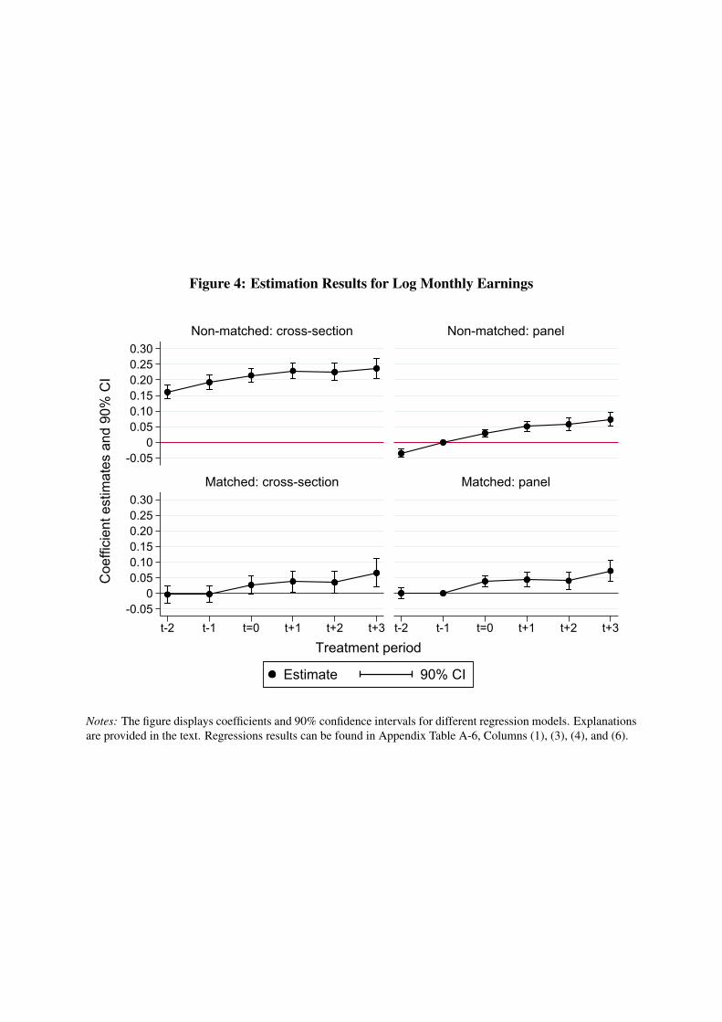
Figure 4: Estimation Results for Log Monthly Earnings

0.300.250.200.150.100.05

0-0.05

0.300.250.200.150.100.05

0-0.05

t-2 t-1 t=0 t+1 t+2 t+3 t-2 t-1 t=0 t+1 t+2 t+3

Non-matched: cross-section Non-matched: panel

Matched: cross-section Matched: panel

Estimate 90% CI

Coe

ffici

ent e

stim

ates

and

90%

CI

Treatment period

Notes: The figure displays coefficients and 90% confidence intervals for different regression models. Explanationsare provided in the text. Regressions results can be found in Appendix Table A-6, Columns (1), (3), (4), and (6).

Figure 5: Estimation Results for Social Capital

-10

0

10

20

30

-10

0

10

20

30

t-2 t-1 t=0 t+1 t+2 t+3 t-2 t-1 t=0 t+1 t+2 t+3



Estimate 90% CI

Coe

ffici

ent e

stim

ates

and

90%

CI

Treatment period

(a) Civic/political participation

-10

0

10

20

30

-10

0

10

20

30

t-2 t-1 t=0 t+1 t+2 t+3 t-2 t-1 t=0 t+1 t+2 t+3



Estimate 90% CI

Coe

ffici

ent e

stim

ates

and

90%

CI

Treatment period

(b) Cultural participation

-10

0

10

20

30

-10

0

10

20

30

t-2 t-1 t=0 t+1 t+2 t+3 t-2 t-1 t=0 t+1 t+2 t+3



Estimate 90% CI

Coe

ffici

ent e

stim

ates

and

90%

CI

Treatment period

(c) Social participation

Notes: The figure displays coefficients and 90% confidence intervals for different regression models. Explanationsare provided in the text. Regressions results can be found in Appendix Tables A-9 to A-11, Columns (1), (3), (4),and (6).

Figure 6: Heterogeneity of Treatment Effects

-1.319

1.999

-0.775

-4.104

-0.772

-1.392

-2.654

0.035

-1.434

8.232**

16.892**

7.450

9.930***

9.420**

9.113

6.006

11.236**

8.868***

10.172**

-6.321

6.821

9.086**

0.757

17.436**

4.962

16.378***

8.605**

-8 -6 -4 -2 0 2 4 6 8 10 12 14 16 18 20

No

Yes

Below

median

Above

median

No

Yes

Male

Female

Baseline


Gender

University

degree

Wage

distribution

Blue collar

worker

(a) Individual characteristics

-0.691

-2.586

-3.190

-1.102

0.406

-4.518

-0.265

-2.260

-0.231

-2.551

8.836*

8.628**

9.805*

8.683***

8.510**

9.747***

7.076*

9.627***

7.607**

10.043***

13.233**

6.893

11.296*

7.584**

8.263**

8.998**

6.371

9.349**

8.321**

9.030**

-8 -6 -4 -2 0 2 4 6 8 10 12 14 16 18 20

Small/

medium

Large

No

Yes

No

Yes

No

Yes

Below

median

Above

median


Employer-

induced

Firm size

Training

intensity

Previous

training

Firm-specific

training

(b) Training characteristics

Notes: The figure shows coefficients on the variable Trainingie × postt+1,t+2,t+3 from baseline regression modelson the subsample indicated. All regressions use entropy-balancing adjusted matching weights to reweight thecomparison group. Baseline weights are used, which are further refined to match within specific subsamples(covariates: log monthly earnings, log hours worked, and the three non-pecuniary outcomes in periods t− 1 andt − 2). Appendix Tables A-18 and A-20 provide regression results. Appendix Tables A-19 and A-21 providetreatment period-specific heterogeneity analysis. Significance level: *** p<0.01, ** p<0.05, * p<0.1.

Table 1: Overview of Conditioning Variables

Demographic characteristicsAgea 3 categories (25-35, 36-45, 46-55)Female 0 = male, 1 = femaleMigrant 1 = individual or parents moved to Germany, 0 elseGerman citizen 1 = German, 0 foreign citizenMarried 1 = yes, 0 = noHomeowner 1 = home owner, 0 = tenantChildren 1 = children under the age of 16 in household, 0 elseSelf-rated healthb (t−1; t−2) 5 categories (1 bad - 5 very good)Federal stated 14 categoriesEvaluation perioda 3 categories (2000, 2004, 2008)Occupational samplea,e 2 categories (blue collar worker; non-blue collar worker)

EducationVocational 0 = no vocational training, 1 = vocational trainingUniversity 0 = no university degree, 1 = university degreeSchooling 4 categories (no degree/basic school; intermediate/other school; technical school;

academic school track (Abitur))Previous work-related training 1 = participated in work-related training before, 0 else

Labor market characteristicsLog monthly earningsc (t−1; t−2) Log monthly gross earnings in 2010 eurosLog hours worked per weekc (t−1; t−2) Log hours worked per weekEarnings tertilea, f 3 categories (bottom; middle; top)Full-time employed (t−1; t−2) 1 = yes, 0 = noOccupational status (t−1; t−2) 7 categories (blue collar; white collar; public servant; self-employed; unemployed;

non-working; apprentice, retired)Civic service (t−1; t−2) 1 = public service, 0 elseUnemployment experience 3 categories (no experience; 0-2 years; more than two years)Tenure with the current firm 4 categories (0-2 years; 2-8 years; 8-15 years; more than 15 years)Firm size (t−1; t−2) 3 categories (small < 20, medium 20-200, large > 200 employees)Industry (t−1; t−2) 10 categories

Satisfaction and worriesLife satisfactionb (t−1; t−2) 11 categories (0 low - 10 high)Worries: economic situationb (t−1; t−2) 3 categories (1 no worries, 2 some worries, 3 big worries)Worries: own economic situationb (t−1; t−2) 3 categories (1 no worries, 2 some worries, 3 big worries)Worries: job situationb (t−1; t−2) 3 categories (1 no worries, 2 some worries, 3 big worries)

Outcomes before treatmentCivic/political participation scorec,g (t−1; t−2) Score from PCACultural participation scorec,g (t−1; t−2) Score from PCASocial participation scorec,g (t−1; t−2) Score from PCA

Interest in politicsb (t−1; t−2) 4 categories (1 not at all - 4 very much)Participate in politicsb (t−1; t−2) 4 categories (1 not at all - 4 very much)Volunteerb (t−1; t−2) 4 categories (1 never - 4 every week)Active in artistic/musical activitiesb (t−1; t−2) 4 categories (1 never - 4 every week)Attend classic eventsb (t−1; t−2) 4 categories (1 never - 4 every week)Attend modern eventsb (t−1; t−2) 4 categories (1 never - 4 every week)Socializeb (t−1; t−2) 4 categories (1 never - 4 every week)Assistb (t−1; t−2) 4 categories (1 never - 4 every week)

Notes: All variables are included for period t−1 if not indicated otherwise. aPropensity score matching is exact on these variables. bVariablex is z-standardized by (x−meanx)/sdx (see Kling et al., 2007). Mean and SD are based on the comparison group in periods t−1 and t−2.cBalancing on first and second moments of these variables in the entropy balancing stage to refine conventional matching weights. dBremenand Hamburg are grouped together with Lower Saxony and Schleswig-Holstein, respectively, due to small samples. eTo belong to theblue-collar worker sample, the individual has to report to work in a blue-collar occupation at least in one year during t− 1 and at least inone year during t−2. To belong to the non-blue-collar worker sample, the individual has to report to work in a white-collar occupation oras a public servant at least in one year during t− 1 and at least in one year during t− 2. Most recent occupation is assigned in the case ofmultiple group membership assignment options. The variable is only used for exact matching and not included in the matching function(instead: matching in detailed occupational status). f Tertiles computed for log monthly gross earnings in 2010 euros averaged over t− 1and t−2. Calculations are based on the sample before matching. gScores are rescaled by evaluation period such that the comparison grouphas, on average, mean 500 and SD 100 in periods t−1 and t−2.

Table 2: Balancing Table – Before Treatment

(1) (2) (3) (4) (5) (6) (7) (8) (9)

Variable Treated Comparison

Non-matched Matched

Mean Mean ∆̃ t-test Mean ∆̃ t-test

coef pvalue coef pvalue

Demographic characteristicsAge: 25-35 0.36 0.31 9.28 0.044 0.000 0.35 2.37 0.011 0.522Age: 35-45 0.44 0.45 -1.60 -0.006 0.567 0.43 1.18 0.006 0.734Age: 45-55 0.21 0.24 -8.61 -0.038 0.000 0.22 -4.18 -0.017 0.245Female 0.42 0.45 -5.90 -0.031 0.019 0.41 1.24 0.006 0.754Migrant 0.12 0.23 -28.18 -0.098 0.000 0.12 0.18 0.001 0.962German citizen 0.97 0.88 34.52 0.085 0.000 0.97 -1.20 -0.002 0.726Married 0.70 0.73 -8.20 -0.034 0.002 0.69 1.54 0.007 0.682Homeowner 0.52 0.47 11.24 0.053 0.000 0.49 5.56 0.028 0.137Children 0.51 0.53 -4.77 -0.021 0.082 0.48 4.90 0.025 0.186East Germany 0.31 0.26 10.55 0.044 0.000 0.30 0.90 0.004 0.823Self-rated health 0.05 0.00 5.00 0.043 0.041 0.06 -1.48 -0.014 0.659Attrition from sample 0.32 0.36 -8.68 -0.039 0.000 0.32 -1.15 -0.005 0.761

EducationDegree: vocational 0.73 0.73 0.08 0.001 0.944 0.75 -4.05 -0.018 0.289Degree: university 0.36 0.17 46.30 0.185 0.000 0.35 1.97 0.009 0.630School degree: no/basic school 0.16 0.34 -41.29 -0.161 0.000 0.16 1.93 0.007 0.608School degree: intermediate/other school 0.42 0.45 -5.94 -0.030 0.020 0.44 -3.45 -0.017 0.376School degree: technical school 0.07 0.04 13.35 0.029 0.000 0.07 -1.23 -0.003 0.759School degree: academic school track (Abitur) 0.33 0.16 41.24 0.162 0.000 0.32 1.85 0.009 0.647School degree: no info 0.01 0.01 0.81 0.000 0.878 0.01 4.43 0.005 0.129Previous work-related traininga 0.66 0.26 87.30 0.371 0.000 0.65 0.97 0.005 0.789

Labor market characteristicsLog gross monthly earnings (in 2010 euro)b 7.93 7.63 51.99 0.279 0.000 7.93 0.00 0.000 1.000Log hours worked per weekb 3.68 3.59 25.57 0.086 0.000 3.68 0.01 0.000 0.998Earnings tertile: bottoma 0.17 0.37 -46.22 -0.184 0.000 0.16 1.05 0.004 0.769Earnings tertile: middlea 0.32 0.34 -5.40 -0.022 0.051 0.32 -1.00 -0.005 0.796Earnings tertile: topa 0.51 0.29 46.98 0.206 0.000 0.51 0.16 0.001 0.968Entry age 19.91 18.40 61.53 1.409 0.000 19.82 3.24 0.083 0.422Employment: full-time 0.84 0.78 15.21 0.058 0.000 0.84 -0.90 -0.003 0.801Employment: part-time 0.14 0.17 -7.80 -0.031 0.000 0.14 0.66 0.002 0.856Employment: marginal/unregular 0.01 0.03 -15.63 -0.019 0.000 0.01 0.09 0.000 0.974Employment: non-working 0.01 0.02 -7.02 -0.008 0.000 0.01 0.57 0.001 0.831Occupation sample: blue collar workera 0.86 0.54 73.58 0.292 0.000 0.85 1.35 0.005 0.709Occupation sample: non-blue collar workera 0.14 0.46 -73.58 -0.292 0.000 0.15 -1.35 -0.005 0.709Civic service 0.41 0.22 42.81 0.178 0.000 0.40 1.48 0.007 0.699Unemployment experience: 0 years 0.71 0.63 17.85 0.076 0.000 0.72 -0.45 -0.002 0.909Unemployment experience: 0-2 years 0.26 0.31 -10.58 -0.043 0.000 0.26 0.59 0.003 0.882Unemployment experience: more than 2 years 0.02 0.06 -18.03 -0.033 0.000 0.03 -0.62 -0.001 0.858Tenure: 0-2 years 0.15 0.17 -4.86 -0.015 0.026 0.14 4.65 0.016 0.105Tenure: 2-8 years 0.35 0.36 -1.84 -0.011 0.265 0.37 -3.01 -0.014 0.357Tenure: 8-15 years 0.26 0.26 0.87 0.006 0.502 0.25 2.16 0.009 0.521Tenure: more than 15 years 0.23 0.20 5.22 0.018 0.066 0.24 -3.00 -0.013 0.433Firm size: small firms (<20) 0.13 0.24 -29.03 -0.100 0.000 0.13 -1.99 -0.007 0.574Firm size: medium firms (20-200) 0.23 0.30 -15.89 -0.065 0.000 0.23 -0.57 -0.002 0.869Firm size: large firms (>200) 0.62 0.42 39.43 0.177 0.000 0.61 1.61 0.008 0.650Firm size: no info 0.03 0.04 -6.88 -0.012 0.000 0.03 0.76 0.001 0.781

Satisfaction and worriesLife satisfaction 0.10 0.03 8.12 0.065 0.001 0.11 -0.78 -0.007 0.815Satisfaction with job situation 0.07 0.01 6.65 0.053 0.007 0.08 -1.76 -0.015 0.597Worries: economic situation 0.09 0.06 2.58 0.008 0.665 0.10 -1.01 -0.009 0.739Worries: own economic situation -0.25 0.00 -25.91 -0.221 0.000 -0.25 0.22 0.002 0.950Worries: job -0.20 0.00 -22.05 -0.190 0.000 -0.21 0.18 0.002 0.959

Non-pecuniary outcomes (before treatment)Civic/political participation scoreb 533 502 29.48 29.202 0.000 533 0.00 -0.005 0.999Cultural participation scoreb 549 502 49.83 42.990 0.000 549 0.00 0.000 1.000Social participation scoreb 501 500 1.35 0.605 0.780 501 0.01 0.010 0.997

Interest in politics 0.40 0.02 39.70 0.350 0.000 0.37 3.14 0.030 0.388Participate in politics 0.16 0.01 14.12 0.145 0.000 0.20 -3.30 -0.040 0.412Volunteer 0.27 0.02 23.84 0.232 0.000 0.25 2.05 0.023 0.583Active in artistic/musical activities 0.30 0.00 29.19 0.280 0.000 0.28 1.77 0.019 0.598Attend classic events 0.41 0.04 39.97 0.339 0.000 0.43 -2.04 -0.019 0.530Attend modern events 0.26 0.01 28.14 0.237 0.000 0.27 -1.10 -0.010 0.752Socialize 0.10 0.01 9.66 0.079 0.000 0.10 -0.14 -0.001 0.967Assist 0.00 0.00 -0.26 -0.007 0.757 0.00 0.48 0.004 0.892

Mean/median/P75 absolute ∆̃ (96 variables) 18.24/9.39/28.60 1.49/1.16/1.98

Notes: The table shows group means before and after matching for treatment and comparison group, averaged over both pretreatment periods t− 1 and t− 2. Appendix Tables A-4 andA-5 show balancing tables separately by treatment period. Sample consists of working-age males and females (25-55 years old), working in each of the two pretreatment periods at leastin one year in a white-collar occupation, a blue-collar occupation, or as a public servant. ∆̃ is the standardized difference in group means. coef and pvalue are based on a regression ofthe specific variable on the treatment indicator and evaluation-period fixed effects. Observations are not weighted before matching and by matching weights after matching. Matchingalso considers ten (plus one for missing) industry dummies, 14 state dummies, and three evaluation period dummies. Variables are not displayed, but included in the average absolutestandardized difference calculations. aExact matching on these variables in the propensity score matching stage. bBalancing on these variables in the entropy balancing stage.

Table 3: Social Capital and Work-Related Training

(1) (2) (3) (4) (5) (6)

Panel A: treatment effects by treatment period


Trainingie × postt+3 10.624** 10.330** 11.047** 10.945** –2.646 –2.506(5.234) (5.218) (4.352) (4.352) (4.868) (4.842)

Trainingie × postt+2 12.273*** 12.301*** 10.774*** 10.449*** –1.481 –0.929(4.435) (4.460) (4.018) (4.022) (4.394) (4.422)

Trainingie × postt+1 4.492 4.493 6.496* 5.597 0.190 0.466(4.147) (4.155) (3.468) (3.421) (3.637) (3.630)

Trainingie × treatt=0 8.567** 8.915*** 3.569 2.667 3.440 3.374(3.402) (3.402) (3.045) (3.051) (3.461) (3.459)

Trainingie × pret−2 0.053 0.147 0.661 0.710 0.298 0.619(3.426) (3.422) (3.137) (3.118) (2.834) (2.830)

R-squared 0.677 0.678 0.601 0.605 0.537 0.539Observations 20,997 20,997 20,997 20,997 20,997 20,997H0: postt+1,t+2 = 0 (pvalue) 0.018 0.018 0.023 0.033 0.886 0.921H0: postt+1,t+2,t+3 = 0 (pvalue) 0.037 0.039 0.031 0.038 0.925 0.925

Panel B: treatment effects averaged over post-treatment periods


Trainingie × postt+1,t+2,t+3 8.605** 8.485** 8.868*** 8.428*** –1.434 –1.267(3.697) (3.710) (3.046) (3.027) (3.579) (3.582)

R-squared 0.657 0.658 0.583 0.588 0.538 0.541Observations 17,159 17,159 17,159 17,159 17,159 17,159

Treatment-by-evaluation FE x x x x x xControl variables x x x x x xIndividual-by-evaluation FE x x x x x xLabor-market control variables x x x

Mean in t−1∩ t−2 533 533 549 549 501 501

Notes: The sample is restricted to male and female individuals who are between 25 and 55 years old. In the matched sample,the comparison group is reweighted to match the treatment group by using entropy-balancing adjusted matching weights.Participation scores are standardized to have mean 500 and standard deviation 100 in the pre-treatment comparison groupfor each evaluation period. In Panel A, Trainingie is equal to one if person i in evaluation period e has participated in atleast ten hours of work-related training in the last three years and zero if the person has not participated in that period.Treatt=0 is equal to one for the averaged three-year treatment period and zero otherwise. Postt+κ indicates averaged post-treatment periods κ = {1,2,3} and Pret−κ indicates averaged pre-treatment periods κ = {1,2}. In Panel B, the variablepostt+1,t+2,t+3 is equal to one if postt+1, postt+2, or postt+3 are equal to one and zero otherwise; period t = 0 is notconsidered. Treatment-by-evaluation FE are treatment period by evaluation period fixed effects and Individual-by-evaluationFE are individual by evaluation period fixed effects (see Figure 1). Control variables: German citizen, married, homeowner,children, vocational degree, university degree, school degree (four categories), state of residence (14 categories), electionsto the national parliament. Labor-market control variables: log monthly earnings, missing earnings dummy, log weeklyhours worked, missing hours worked dummy, employment status (six categories), occupational status (eight categories),civil service, unemployment experience (three categories), tenure (four categories)), industry (ten categories)), and firm size(three categories). All regressions contain dummy variables for outcome scores that are based on imputed socialize, assist,and active values. Mean in t− 1∩ t− 2 is computed for the comparison group. Standard errors, clustered at the individuallevel, in parentheses. Significance level: *** p<0.01, ** p<0.05, * p<0.1.

Table 4: Common Trends in Pretreatment Period

(1) (2) (3) (4) (5) (6) (7) (8)

Log earnings Civic/political Cultural Social

Attrition in t +2/t +3 Attrition in t +2/t +3 Attrition in t +2/t +3 Attrition in t +2/t +3

No Yes No Yes No Yes No Yes

Panel A: non-matched sample

Trainingie × pret−3 –0.060*** –0.047*** –1.900 0.779 2.631 1.017 0.179 2.649(0.014) (0.010) (3.354) (2.510) (2.820) (2.126) (3.636) (2.789)

R-squared 0.841 0.859 0.676 0.693 0.700 0.694 0.568 0.577Observations 14,966 26,744 14,869 26,567 14,869 26,567 14,869 26,567

Panel B: matched sample

Trainingie × pret−3 –0.011 –0.012 1.993 5.317 –0.426 –0.816 –3.182 0.347(0.021) (0.015) (4.858) (3.999) (4.330) (3.338) (5.476) (4.179)


Treatment-by-evaluation FE x x x x x x x xIndividual-by-evaluation FE x x x x x x x x

Mean in t−1∩ t−2 7.933 7.933 533 533 549 549 501 501

Notes: The sample is restricted to the three pre-treatment periods. Pret−3 is equal to one if the period is equal to pre-treatment period 3 and zero if the period is equal to pre-treatmentperiods 1 or 2, respectively. Attrition in t +2/t +3: no indicates that individuals are dropped when they do not report a participation score. Attrition in t +2/t +3: yes allows individualsto report a participation score in one of the periods only. In the matched sample, the comparison group is reweighted to match the treatment group by using entropy-balancing adjustedmatching weights. Table 3 provides further information on the sample and the variables. Standard errors, clustered at the individual level, in parentheses. Significance level: *** p<0.01,** p<0.05, * p<0.1.

Table 5: Heterogeneity by Monetary Value of the Training

(1) (2) (3) (4) (5) (6) (7) (8)

Log earnings Civic/political Cultural Social

Monetary value Monetary value Monetary value Monetary value

High Low High Low High Low High Low


Trainingie × postt+3 0.152*** –0.002 5.441 14.994** 11.982** 10.344* –8.117 3.336(0.027) (0.029) (6.744) (6.543) (5.573) (5.389) (6.167) (6.100)

Trainingie × postt+2 0.126*** –0.041* 10.938* 14.025** 9.635** 11.445** 0.265 –1.839(0.019) (0.024) (5.865) (5.641) (4.875) (5.074) (5.174) (5.421)

Trainingie × postt+1 0.100*** –0.015 3.577 5.658 8.051* 5.816 –1.619 2.533(0.015) (0.023) (5.519) (5.354) (4.502) (4.401) (4.418) (4.816)

Trainingie × treatt=0 0.060*** 0.019 7.621 10.741** 1.459 5.893 4.276 3.068(0.012) (0.016) (4.710) (4.205) (3.925) (3.754) (4.431) (4.453)

Trainingie × pret−2 –0.000 0.003 –0.019 0.147 0.083 1.135 0.112 0.184(0.013) (0.014) (4.307) (4.214) (4.218) (3.540) (3.271) (3.918)

R-squared 0.759 0.722 0.683 0.667 0.598 0.601 0.554 0.520Observations 14,270 14,044 14,419 14,351 14,419 14,351 14,419 14,351H0: postt+1,t+2 = 0 (pvalue) 0.000 0.203 0.149 0.039 0.094 0.079 0.888 0.555H0: postt+1,t+2,t+3 = 0 (pvalue) 0.000 0.209 0.269 0.052 0.118 0.124 0.380 0.652


Trainingie × postt+1,t+2,t+3 0.123*** –0.021 6.303 10.893** 10.055*** 7.993** –2.693 0.633(0.017) (0.022) (4.841) (4.737) (3.689) (3.879) (4.171) (4.567)


Treatment-by-evaluation FE x x x x x x x xControl variables x x x x x x x xIndividual-by-evaluation FE x x x x x x x x

Mean absolute ∆̃ 3.84 2.61 3.84 2.61 3.84 2.61 3.84 2.61Median absolute ∆̃ 3.22 2.19 3.22 2.19 3.22 2.19 3.22 2.19P75 absolute ∆̃ 5.74 3.98 5.74 3.98 5.74 3.98 5.74 3.98

Notes: The table splits the treatment group into two categories: training participants whose hourly earnings have increased more than in the comparisongroup (group high) and training participants whose hourly earnings have increased not more than in the comparison group (group low). All regressions useentropy-balancing adjusted matching weights to reweight the comparison group. Baseline weights are used, which are further refined to match within specificsubsamples (covariates: log monthly earnings, log hours worked, and the three non-pecuniary outcomes in periods t−1 and t−2). Standard errors, clustered atthe individual level, in parentheses. Significance level: *** p<0.01, ** p<0.05, * p<0.1.

Table 6: Robustness Checks

(1) (2) (3) (4) (5) (6) (7)

Baseline (PSM with refinement by EB) PSM EB

Baseline Trends Notrimming

NN Baseline Trends

Panel A: civic/political participation

Trainingie × postt+1,t+2,t+3 8.605** 8.139** 7.593** 6.608** 9.380** 6.612** 6.599**(3.697) (3.749) (3.364) (3.026) (3.755) (2.762) (2.768)

R-squared 0.657 0.660 0.676 0.672 0.650 0.674 0.673

Panel B: cultural participation

Trainingie × postt+1,t+2,t+3 8.868*** 9.603*** 7.976*** 6.721*** 8.615*** 7.202*** 7.524***(3.046) (3.080) (2.777) (2.455) (3.140) (2.401) (2.383)

R-squared 0.583 0.581 0.592 0.582 0.582 0.592 0.593

Panel C: social participation

Trainingie × postt+1,t+2,t+3 –1.434 –1.153 1.174 –0.997 –2.571 1.675 1.954(3.579) (3.661) (3.448) (2.921) (3.598) (2.788) (2.781)

R-squared 0.538 0.539 0.541 0.543 0.540 0.546 0.547

Treatment-by-evaluation FE x x x x x x xControl variables x x x x x x xIndividual-by-evaluation FE x x x x x x x

Observations 17,159 17,159 18,256 25,486 17,159 40,035 40,035

Mean absolute ∆̃ 1.49 1.66 1.77 1.15 1.45 0.34 0.79Median absolute ∆̃ 1.14 1.27 1.39 0.90 1.13 0.10 0.65P75 absolute ∆̃ 1.96 2.13 2.27 1.83 2.11 0.43 1.10

Notes: The table shows averaged treatment effects under different model specifications. The variable postt+1,t+2,t+3 is equal to one if postt+1,postt+2, or postt+3 are equal to one and zero otherwise; period t = 0 is not considered. Column (2): use entropy balancing to further refinethe baseline weights (used in Column (1)) by adjusting for trends in the outcome variables (log monthly earnings, log hours worked perweek, three non-pecuniary outcome scores) by previous work-related training, university degree, vocational degree, gender, and occupationsample. Column (3): sample is not trimmed after calculating the propensity scores. Column (4): use 5-to-1 nearest-neighbor matchinginstead of kernel matching. Column (5): use matching weights from propensity score matching without further refinement. Column (6):use only entropy balancing on same covariates as in the baseline model (Column (1)). Column (6): use only entropy balancing on samecovariates as in Column (1) with further refinement of the weights by adjusting for trends in the outcome variables (log monthly earnings,log hours worked per week, three non-pecuniary outcome scores) by previous work-related training, university degree, vocational degree,gender, and occupation sample. Appendix Table A-17 provides treatment period-specific results. Standard errors, clustered at the individuallevel, in parentheses. Significance level: *** p<0.01, ** p<0.05, * p<0.1.

A Appendix Figures and Tables

Figure A-1: Start Years of Work-Related Training Courses

0

0.10

0.20

0.30

0.40

0.50

0.60

t t-1 t-2 t-3 t-4 t-5 t-6

1 2 3 1 2 3 1 2 3 1 2 3 1 2 3 1 2 3 1 2 3

Notes: The figure shows the distribution of start years (relative to the qualification survey) for the last three coursesof the individual.

Figure A-2: Non-Pecuniary Outcome Scores by Position in the Monthly EarningsDistribution

480

500

520

540

560

0 20 40 60 80 100

Earnings percentile


Notes: The figure shows average values of the three non-pecuniary outcome variables by position of the individualin the monthly earnings distribution. Earnings are in 2010 euro.

Figure A-3: Distribution of Courses and Course Hours

0

0.1

0.2

0.3

Den

sity

0 1 2 3 4 5 6 7 8 9 10 11 12 13 14 15

Number of courses, last three years

Average 2000 2004 2008

(a) Number of courses (pdf)

0

0.25

0.50

0.75

1

0 3 5 10 15 20 25 30 35 40

Number of courses, last three years

Average 2000 2004 2008

(b) Number of courses (cdf)

0

0.01

0.02

0.03

0.04

Den

sity

0 10 20 30 40 50 60 70 80 90 100


Average 2000 2004 2008

(c) Number of course hours (pdf)

0

0.25

0.50

0.75

1

10 50 100 150 200 250 300 350

Number of training hours, last three years

Average 2000 2004 2008

(d) Number of course hours (cdf)

Notes: The figures show the distribution of courses and course hours. Distributions are based on the sample in thepretreatment period t−1. For illustrative purpose, distributions are capped at the last value displayed. For numberof courses in Figures A-3(a) and A-3(b), the mean is equal to 3.9, the median is equal to 3, and the largest value isequal to 99. Figure A-3(c) shows the distribution of course hours after restricting the sample to individuals with atleast 10 hours of training. Figure A-3(d) provides the CDF for the unrestricted sample. The mean in the restricted(unrestricted) sample is equal to 208 (149), the median is equal to 33 (22), and the largest value is equal to 13,757.

Figure A-4: Distribution of Employer- and Non-Employer-Induced Course Hours

0

0.01

0.02

0.03

0.04

Den

sity

10 20 30 40 50 60 70 80 90 100


All coursesEmployer-induced Non-employer-induced

Notes: The figure shows the distribution of individual training course hours. Individual training course hoursare calculated as the sum of the three reported training courses. The distribution is based on the sample in thepretreatment period t− 1. For illustrative purpose, the distribution is capped at 100 course hours. An individualhas participated in employer-induced courses if the majority of training courses took place during work-time, arefinanced by the employer, or organized and hosted by the employer.

Figure A-5: Descriptive Relationship between Work-Related Training and Earnings

7.5

7.6

7.7

7.8

7.9

8.0

8.1

Log

mon

thly

gro

ss e

arni

ngs

(201

0 eu

ro)

t-3 t-2 t-1 t t+1 t+2 t+3

Treatment period

Matched Non-matchedTreated Comparison Treated Comparison

(a) Log monthly earnings

0.98

0.99

1

1.01

1.02

1.03

Log

mon

thly

gro

ss e

arni

ngs

(201

0 eu

ro, r

elat

ive

to p

erio

d t)

t-3 t-2 t-1 t t+1 t+2 t+3

Treatment period


(b) Log monthly earnings relative to pretreatment period t−1

Notes: The figures show treatment-period averages of log monthly gross earnings. Observations in the comparisongroup are weighted by matching weights in the matched sample.

Figure A-6: Descriptive Relationship between Work-Related Training and ParticipationDomains

490

500

510

520

530

540

550

560

t-3 t-2 t-1 t t+1 t+2 t+3

Treatment period


(a) Civic/political participation

490

500

510

520

530

540

550

560

t-3 t-2 t-1 t t+1 t+2 t+3

Treatment period


(b) Cultural participation

490

500

510

520

530

540

550

560

t-3 t-2 t-1 t t+1 t+2 t+3

Treatment period


(c) Social participation

Notes: The figures show treatment-period averages of participation scores. Observations in the comparison groupare weighted by matching weights in the matched sample.

Figure A-7: Treatment-Period Averages of Subdimensions

-0.20

-0.10

0

0.10

0.20

0.30

0.40

0.50

0.60

0.70

t-3 t-2 t-1 t t+1 t+2 t+3

Treatment period


(a) Interest in politics

-0.20

-0.10

0

0.10

0.20

0.30

0.40

0.50

0.60

0.70

t-3 t-2 t-1 t t+1 t+2 t+3

Treatment period


(b) Participate in politics

-0.20

-0.10

0

0.10

0.20

0.30

0.40

0.50

0.60

0.70

t-3 t-2 t-1 t t+1 t+2 t+3

Treatment period


(c) Volunteer

-0.20

-0.10

0

0.10

0.20

0.30

0.40

0.50

0.60

0.70

t-3 t-2 t-1 t t+1 t+2 t+3

Treatment period


(d) Attend cultural events

-0.20

-0.10

0

0.10

0.20

0.30

0.40

0.50

0.60

0.70

t-3 t-2 t-1 t t+1 t+2 t+3

Treatment period


(e) Attend modern events

-0.20

-0.10

0

0.10

0.20

0.30

0.40

0.50

0.60

0.70

t-3 t-2 t-1 t t+1 t+2 t+3

Treatment period


(f) Active

-0.20

-0.10

0

0.10

0.20

0.30

0.40

0.50

0.60

0.70

t-3 t-2 t-1 t t+1 t+2 t+3

Treatment period


(g) Socialize

-0.20

-0.10

0

0.10

0.20

0.30

0.40

0.50

0.60

0.70

t-3 t-2 t-1 t t+1 t+2 t+3

Treatment period


(h) Assist

Notes: The figures show treatment-period averages of participation scores. Observations in the comparison groupare weighted by matching weights in the matched sample.

Table A-1: Correlation Matrix of Participation Variables

Variable (1) (2) (3) (4) (5) (6) (7) (8)

(1) Interest in politics 1.000(2) Participate in politics 0.230 1.000(3) Volunteer 0.137 0.349 1.000(4) Active in artistic/musical activities 0.120 0.142 0.204 1.000(5) Attend classic events 0.224 0.171 0.199 0.319 1.000(6) Attend modern events 0.133 0.059 0.115 0.182 0.399 1.000(7) Socialize 0.049 0.033 0.087 0.109 0.157 0.219 1.000(8) Assist 0.006 0.073 0.158 0.049 0.083 0.112 0.387 1.000

Notes: The table shows the correlation matrix of outcome variables. The sample for these calculations is restricted toobservations in the comparison group in pre-treatment periods t−1 and t−2. No imputations are used for the calculations.

Table A-2: Rotated Components

Variable Non-pecuniary outcome dimensions


Interest in politics 0.324 0.243 –0.170Participate in politics 0.682 –0.052 –0.022Volunteer 0.604 –0.008 0.126Active in artistic/musical activities 0.129 0.426 –0.062Attend classic events 0.043 0.610 –0.037Attend modern events –0.170 0.597 0.100Socialize –0.074 0.138 0.652Assist 0.097 –0.083 0.716

Notes: The table shows the rotations from the principal component analysis of the outcome variables. Thesample for these calculations is restricted to observations in the comparison group in pre-treatment periods t−1and t−2. No imputations are used for the calculations.

Table A-3: Sample Size for Subsamples with the Propensity Score between 0.1 and 0.9

(1) (2) (3) (4)

Low Middle High AllP < 0.1 0.1≤ P≤ 0.9 P > 0.9

Comparison 2,300 4,598 0 6,898Treatment 124 2,533 0 2,657All 2,424 7,131 0 9,555

Notes: The table shows sample sizes for subsamples that have a very low probability to participate in training (P < 0.1) anda very high probability to participate in training (P > 0.9). We drop those individuals from the analysis. Sample is based onpretreatment period t−1. Number of unique persons is equal to 6,492. Treatment covers individuals who have participatedin at least ten hours of work-related training in the last three years. Comparison covers individuals who have not participatedin any work-related training in the last three years.

Table A-4: Balancing Table – Before Treatment (period t−1)

(1) (2) (3) (4) (5) (6) (7) (8) (9)


Non-matched Matched



Demographic characteristicsAge: 25-35 0.31 0.27 8.75 0.039 0.000 0.31 0.18 0.001 0.962Age: 35-45 0.45 0.45 -0.10 0.002 0.854 0.43 2.93 0.015 0.431Age: 45-55 0.25 0.28 -8.87 -0.041 0.000 0.26 -3.54 -0.015 0.353Female 0.42 0.45 -5.90 -0.031 0.019 0.41 1.24 0.006 0.754Migrant 0.12 0.23 -28.18 -0.098 0.000 0.12 0.18 0.001 0.962German citizen 0.97 0.88 34.00 0.082 0.000 0.97 -1.72 -0.003 0.617Married 0.71 0.74 -8.49 -0.036 0.002 0.71 -1.14 -0.005 0.771Homeowner 0.54 0.48 11.76 0.055 0.000 0.52 4.85 0.024 0.216Children 0.50 0.51 -3.13 -0.013 0.308 0.47 4.84 0.024 0.214East Germany 0.31 0.26 10.39 0.043 0.000 0.31 0.54 0.003 0.893Self-rated health 0.02 -0.04 5.88 0.052 0.026 0.02 -0.96 -0.009 0.798Attrition from sample 0.32 0.36 -8.59 -0.039 0.000 0.32 -1.15 -0.005 0.761

EducationDegree: vocational 0.73 0.73 1.08 0.006 0.621 0.75 -4.32 -0.019 0.274Degree: university 0.37 0.17 46.85 0.187 0.000 0.36 2.07 0.010 0.615School degree: no/basic school 0.16 0.33 -41.90 -0.162 0.000 0.15 1.58 0.006 0.681School degree: intermediate/other school 0.42 0.46 -6.69 -0.034 0.009 0.44 -3.76 -0.019 0.342School degree: technical school 0.08 0.04 14.23 0.031 0.000 0.08 -1.16 -0.003 0.779School degree: academic school track (Abitur) 0.33 0.16 41.74 0.164 0.000 0.32 2.47 0.012 0.542School degree: no info 0.01 0.01 0.67 0.000 0.908 0.01 4.12 0.004 0.170Previous work-related traininga 0.66 0.26 87.29 0.371 0.000 0.65 0.97 0.005 0.789

Labor market characteristicsLog gross monthly earnings (in 2010 euro)b 7.97 7.65 55.97 0.297 0.000 7.97 0.00 0.000 1.000Log hours worked per weekb 3.69 3.59 27.18 0.090 0.000 3.69 0.01 0.000 0.998Earnings tertile: bottoma 0.17 0.37 -46.22 -0.184 0.000 0.16 1.05 0.004 0.769Earnings tertile: middlea 0.32 0.34 -5.40 -0.022 0.051 0.32 -1.00 -0.005 0.796Earnings tertile: topa 0.51 0.29 46.98 0.206 0.000 0.51 0.16 0.001 0.968Entry age 19.91 18.40 61.52 1.409 0.000 19.82 3.24 0.083 0.422Employment: full-time 0.84 0.78 14.80 0.058 0.000 0.84 -0.20 -0.001 0.960Employment: part-time 0.15 0.17 -6.61 -0.027 0.003 0.15 -0.05 0.000 0.990Employment: apprenticeship 0.00 0.00 -2.95 0.000 0.084 0.00 0.000Employment: marginal/unregular 0.01 0.03 -19.52 -0.023 0.000 0.01 -1.55 -0.001 0.632Employment: non-working 0.01 0.02 -5.85 -0.007 0.008 0.01 2.11 0.002 0.546Occupation sample: blue collar worker 0.86 0.54 73.64 0.292 0.000 0.85 1.35 0.005 0.709Occupation sample: non-blue collar worker 0.14 0.46 -73.64 -0.292 0.000 0.15 -1.35 -0.005 0.709Civil service 0.41 0.21 43.95 0.182 0.000 0.41 1.79 0.009 0.654Unemployment experience: 0 years 0.71 0.62 18.35 0.078 0.000 0.71 -0.61 -0.003 0.877Unemployment experience: 0-2 years 0.27 0.32 -10.94 -0.045 0.000 0.26 0.50 0.002 0.900Unemployment experience: more than 2 years 0.03 0.06 -17.94 -0.033 0.000 0.03 0.11 0.000 0.975Tenure: 0-2 years 0.11 0.14 -8.58 -0.024 0.001 0.11 1.00 0.003 0.777Tenure: 2-8 years 0.36 0.36 -0.64 -0.006 0.607 0.36 -0.94 -0.005 0.804Tenure: 8-15 years 0.28 0.28 0.74 0.006 0.580 0.27 2.34 0.010 0.536Tenure: more than 15 years 0.25 0.22 6.24 0.023 0.034 0.26 -2.35 -0.010 0.553Firm size: small firms (<20) 0.12 0.24 -31.47 -0.106 0.000 0.13 -2.94 -0.010 0.435Firm size: medium firms (20-200) 0.24 0.30 -15.30 -0.064 0.000 0.24 -0.67 -0.003 0.859Firm size: large firms (>200) 0.62 0.42 40.54 0.181 0.000 0.61 1.88 0.009 0.625Firm size: no info 0.02 0.04 -6.80 -0.011 0.002 0.02 2.33 0.003 0.483

Satisfaction and worriesLife satisfaction 0.10 0.01 9.69 0.078 0.001 0.09 0.69 0.006 0.852Satisfaction with job situation 0.04 -0.01 5.56 0.046 0.042 0.05 -1.44 -0.013 0.711Worries: economic situation 0.08 0.05 2.89 0.005 0.833 0.11 -2.69 -0.025 0.444Worries: own economic situation -0.27 -0.01 -27.30 -0.241 0.000 -0.28 0.32 0.003 0.935Worries: job -0.19 0.01 -21.41 -0.193 0.000 -0.19 -0.08 -0.001 0.982

Non-pecuniary outcomes (before treatment)Civic/political participation scoreb 534 502 29.26 29.458 0.000 534 -0.01 -0.007 0.999Cultural participation scoreb 550 503 50.29 43.115 0.000 550 0.00 0.000 1.000Social participation scoreb 503 502 1.54 0.462 0.840 503 0.01 0.010 0.998Interest in politics 0.38 -0.01 40.35 0.359 0.000 0.35 3.90 0.038 0.313Participate in politics 0.14 -0.01 14.05 0.144 0.000 0.18 -3.12 -0.038 0.466Volunteer 0.31 0.05 24.74 0.245 0.000 0.30 1.55 0.017 0.697Active in artistic/musical activities 0.24 -0.05 28.48 0.267 0.000 0.22 2.03 0.022 0.581Attend classic events 0.52 0.16 38.30 0.330 0.000 0.55 -3.43 -0.032 0.367Attend modern events 0.22 -0.05 31.25 0.254 0.000 0.22 -0.18 -0.002 0.963Socialize 0.11 0.02 9.70 0.075 0.001 0.11 -0.16 -0.001 0.966Assist 0.02 0.02 -0.35 -0.010 0.661 0.01 0.51 0.005 0.892


Notes: The table shows group means before and after matching for treatment and comparison group for pretreatment period t−1. Sample consists of working-age males and females (25-55years old), working in each of the two pretreatment periods at least in one year in a white collar occupation, a blue collar occupation, or as a public servant. ∆̃ is the standardized differencein group means. coef and pvalue are based on a regression of the specific variable on the treatment indicator and evaluation-period fixed effects. Observations are not weighted beforematching and by matching weights after matching. Matching also considers ten (plus one for missing) industry dummies, 14 state dummies, and three evaluation period dummies. Variablesare not displayed, but included in the average absolute standardized difference calculations. aExact matching on these variables in the propensity score matching stage. bBalancing onthese variables in the entropy balancing stage.

Table A-5: Balancing Table – Before Treatment (period t−2)

(1) (2) (3) (4) (5) (6) (7) (8) (9)


Non-matched Matched



Demographic characteristicsAge: 25-35 0.41 0.36 9.87 0.048 0.000 0.38 4.45 0.022 0.250Age: 35-45 0.43 0.44 -3.10 -0.014 0.223 0.43 -0.58 -0.003 0.879Age: 45-55 0.17 0.20 -8.45 -0.034 0.000 0.18 -4.97 -0.019 0.190Female 0.42 0.45 -5.90 -0.031 0.019 0.41 1.24 0.006 0.754Migrant 0.12 0.23 -28.18 -0.098 0.000 0.12 0.18 0.001 0.962German citizen 0.97 0.87 35.04 0.087 0.000 0.97 -0.69 -0.001 0.842Married 0.69 0.72 -7.92 -0.033 0.005 0.67 4.15 0.019 0.288Homeowner 0.50 0.45 10.74 0.051 0.000 0.47 6.28 0.031 0.105Children 0.52 0.55 -6.42 -0.029 0.021 0.49 4.97 0.025 0.201East Germany 0.31 0.26 10.70 0.045 0.000 0.30 1.26 0.006 0.756Self-rated health 0.09 0.05 4.10 0.034 0.141 0.10 -2.02 -0.018 0.591Attrition from sample 0.32 0.36 -8.77 -0.038 0.000 0.32 -1.15 -0.005 0.761

EducationDegree: vocational 0.73 0.73 -0.92 -0.004 0.721 0.75 -3.79 -0.017 0.333Degree: university 0.36 0.16 45.75 0.182 0.000 0.35 1.87 0.009 0.649School degree: no/basic school 0.17 0.34 -40.70 -0.161 0.000 0.16 2.27 0.008 0.551School degree: intermediate/other school 0.43 0.45 -5.20 -0.026 0.047 0.44 -3.15 -0.016 0.425School degree: technical school 0.07 0.04 12.44 0.026 0.000 0.07 -1.29 -0.003 0.748School degree: academic school track (Abitur) 0.33 0.16 40.74 0.160 0.000 0.32 1.22 0.006 0.764School degree: no info 0.01 0.01 0.95 0.000 0.868 0.01 4.76 0.005 0.143Previous work-related traininga 0.66 0.26 87.29 0.371 0.000 0.65 0.97 0.005 0.789

Labor market characteristicsLog gross monthly earnings (in 2010 euro)b 7.90 7.61 48.18 0.261 0.000 7.90 0.00 0.000 1.000Log hours worked per weekb 3.67 3.58 24.03 0.082 0.000 3.67 0.01 0.000 0.999Earnings tertile: bottoma 0.17 0.37 -46.22 -0.184 0.000 0.16 1.05 0.004 0.769Earnings tertile: middlea 0.32 0.34 -5.40 -0.022 0.051 0.32 -1.00 -0.005 0.796Earnings tertile: topa 0.51 0.29 46.98 0.206 0.000 0.51 0.16 0.001 0.968Entry age 19.91 18.40 61.52 1.409 0.000 19.82 3.24 0.083 0.422Employment: full-time 0.84 0.78 15.62 0.059 0.000 0.85 -1.62 -0.006 0.671Employment: part-time 0.14 0.17 -9.01 -0.035 0.000 0.13 1.40 0.005 0.716Employment: apprenticeship 0.00 0.00 0.80 0.000 0.774 0.00 3.97 0.001 0.157Employment: marginal/unregular 0.01 0.03 -12.20 -0.015 0.000 0.01 1.21 0.001 0.736Employment: non-working 0.01 0.02 -8.18 -0.009 0.000 0.01 -0.95 -0.001 0.785Occupation sample: blue collar worker 0.86 0.54 73.50 0.292 0.000 0.85 1.35 0.005 0.709Occupation sample: non-blue collar worker 0.14 0.46 -73.50 -0.292 0.000 0.15 -1.35 -0.005 0.709Civil service 0.41 0.22 41.68 0.174 0.000 0.40 1.18 0.006 0.768Unemployment experience: 0 years 0.72 0.64 17.35 0.073 0.000 0.72 -0.28 -0.001 0.943Unemployment experience: 0-2 years 0.25 0.30 -10.21 -0.041 0.000 0.25 0.68 0.003 0.865Unemployment experience: more than 2 years 0.02 0.06 -18.15 -0.032 0.000 0.02 -1.40 -0.002 0.693Tenure: 0-2 years 0.20 0.20 -1.91 -0.007 0.464 0.17 7.68 0.030 0.032Tenure: 2-8 years 0.35 0.36 -3.04 -0.015 0.161 0.37 -5.07 -0.024 0.179Tenure: 8-15 years 0.25 0.25 1.01 0.007 0.504 0.24 1.98 0.009 0.598Tenure: more than 15 years 0.20 0.19 4.15 0.014 0.157 0.22 -3.69 -0.015 0.353Firm size: small firms (<20) 0.14 0.24 -26.64 -0.094 0.000 0.14 -1.08 -0.004 0.771Firm size: medium firms (20-200) 0.22 0.29 -16.50 -0.066 0.000 0.22 -0.46 -0.002 0.903Firm size: large firms (>200) 0.61 0.42 38.33 0.172 0.000 0.60 1.35 0.007 0.723Firm size: no info 0.03 0.04 -6.98 -0.013 0.002 0.03 -0.56 -0.001 0.888

Satisfaction and worriesLife satisfaction 0.11 0.05 6.48 0.052 0.018 0.13 -2.28 -0.020 0.539Satisfaction with job situation 0.10 0.03 7.82 0.059 0.006 0.11 -2.11 -0.018 0.568Worries: economic situation 0.09 0.07 2.24 0.011 0.582 0.08 0.82 0.007 0.816Worries: own economic situation -0.22 0.01 -24.48 -0.201 0.000 -0.22 0.12 0.001 0.975Worries: job -0.22 -0.01 -22.71 -0.187 0.000 -0.22 0.45 0.004 0.905

Non-pecuniary outcomes (before treatment)Civic/political participation scoreb 533 501 29.71 28.945 0.000 533 0.00 -0.004 0.999Cultural participation scoreb 548 501 49.36 42.865 0.000 548 0.00 0.000 1.000Social participation scoreb 499 498 1.16 0.748 0.746 499 0.01 0.011 0.998Interest in politics 0.42 0.05 39.06 0.342 0.000 0.40 2.36 0.022 0.544Participate in politics 0.18 0.03 14.19 0.146 0.000 0.23 -3.47 -0.042 0.424Volunteer 0.23 0.00 22.95 0.220 0.000 0.21 2.57 0.028 0.522Active in artistic/musical activities 0.37 0.04 29.95 0.294 0.000 0.35 1.53 0.017 0.680Attend classic events 0.30 -0.08 42.44 0.347 0.000 0.30 -0.61 -0.005 0.870Attend modern events 0.30 0.07 25.28 0.220 0.000 0.31 -1.99 -0.018 0.612Socialize 0.09 -0.01 9.62 0.083 0.000 0.09 -0.13 -0.001 0.972Assist -0.01 -0.01 -0.17 -0.003 0.890 -0.02 0.44 0.004 0.908


Notes: The table shows group means before and after matching for treatment and comparison group for pretreatment period t−2. Sample consists of working-age males and females (25-55years old), working in each of the two pretreatment periods at least in one year in a white collar occupation, a blue collar occupation, or as a public servant. ∆̃ is the standardized differencein group means. coef and pvalue are based on a regression of the specific variable on the treatment indicator and evaluation-period fixed effects. Observations are not weighted beforematching and by matching weights after matching. Matching also considers ten (plus one for missing) industry dummies, 14 state dummies, and three evaluation period dummies. Variablesare not displayed, but included in the average absolute standardized difference calculations. aExact matching on these variables in the propensity score matching stage. bBalancing onthese variables in the entropy balancing stage.

Table A-6: Work-Related Training and Log Monthly Earnings (in 2010 euro)

(1) (2) (3) (4) (5) (6) (7)

Dependent variable: log monthly gross earnings (in 2010 euros)

Non-matched sample Matched sample

Trainingie × postt+3 0.344*** 0.237*** 0.074*** 0.084*** 0.066** 0.072*** 0.049***(0.020) (0.019) (0.014) (0.031) (0.027) (0.021) (0.016)

Trainingie × postt+2 0.333*** 0.226*** 0.058*** 0.050** 0.035 0.040** 0.031**(0.017) (0.017) (0.012) (0.025) (0.021) (0.017) (0.014)

Trainingie × postt+1 0.338*** 0.229*** 0.051*** 0.049** 0.038* 0.044*** 0.031**(0.016) (0.016) (0.009) (0.024) (0.021) (0.014) (0.012)

Trainingie × treatt=0 0.320*** 0.215*** 0.030*** 0.029 0.027 0.039*** 0.020**(0.015) (0.014) (0.007) (0.021) (0.018) (0.011) (0.009)

Trainingie × pret−1 0.297*** 0.192*** [baseline] 0.000 –0.003 [baseline] [baseline](0.014) (0.014) (0.019) (0.017)

Trainingie × pret−2 0.261*** 0.161*** –0.035*** 0.000 –0.004 0.001 0.004(0.014) (0.014) (0.008) (0.020) (0.018) (0.010) (0.009)

Treatment-by-evaluation FE x x x x x x xControl variables x x x x xIndividual-by-evaluation FE x x xLabor-market control variables x

R-squared 0.054 0.168 0.835 0.024 0.193 0.797 0.862Observations 47,789 47,789 47,789 20,695 20,695 20,695 20,596Mean in t−1∩ t−2 7.630 7.630 7.630 7.933 7.933 7.933 7.933H0: postt+1,t+2 = 0 (pvalue) 0.000 0.000 0.000 0.091 0.160 0.006 0.023H0: postt+1,t+2,t+3 = 0 (pvalue) 0.000 0.000 0.000 0.063 0.103 0.003 0.015

Notes: The sample is restricted to male and female individuals who are between 25 and 55 years old. In the matched sample, the comparison group is reweighted to match the treatmentgroup by using entropy-balancing adjusted matching weights. Trainingie is equal to one if person i in evaluation period e has participated in at least ten hours of work-related training in thelast three years and zero if the person has not participated in that period. Treatt=0 is equal to one for the averaged three-year treatment period and zero otherwise. Postt+κ indicates averagedposttreatment periods κ = {1,2,3} and Pret−κ indicates averaged pretreatment periods κ = {1,2}. Treatment-by-evaluation FE are treatment period by evaluation period fixed effects andIndividual-by-evaluation FE are individual by evaluation period fixed effects (see Figure 1). Control variables: German citizen, married, homeowner, children, vocational degree, universitydegree, school degree (four categories), state of residence (14 categories), elections to the national parliament. Labor-market control variables: log weekly hours worked, employment status (sixcategories), occupational status (eight categories), civil service, unemployment experience (three categories), tenure (four categories), industry (ten categories), and firm size (three categories).Mean in t−1∩ t−2 is computed for the comparison group. Standard errors, clustered at the individual level, in parentheses. Significance level: *** p<0.01, ** p<0.05, * p<0.1.

Table A-7: Work-Related Training and Log Hourly Earnings (in 2010 euro)

(1) (2) (3) (4) (5) (6) (7)

Dependent variable: log hourly earnings (in 2010 euros)


Trainingie × postt+3 0.243*** 0.156*** 0.062*** 0.044* 0.029 0.049*** 0.046***(0.016) (0.014) (0.012) (0.024) (0.020) (0.018) (0.017)

Trainingie × postt+2 0.240*** 0.152*** 0.048*** 0.035* 0.020 0.022 0.022(0.014) (0.012) (0.010) (0.020) (0.016) (0.015) (0.014)

Trainingie × postt+1 0.243*** 0.155*** 0.040*** 0.034* 0.024 0.027** 0.024*(0.013) (0.012) (0.009) (0.019) (0.016) (0.013) (0.013)

Trainingie × treatt=0 0.216*** 0.133*** 0.012 0.004 0.004 0.010 0.009(0.011) (0.010) (0.007) (0.016) (0.013) (0.010) (0.010)


Trainingie × pret−2 0.178*** 0.101*** –0.027*** –0.001 –0.002 –0.000 0.002(0.011) (0.010) (0.007) (0.015) (0.013) (0.010) (0.010)

Treatment-by-evaluation period FE x x x x x x xControl variables x x x x xIndividual-by-evaluation period FE x x xLabor-market control variables x

R-squared 0.055 0.255 0.755 0.029 0.267 0.743 0.750Observations 47,512 47,512 47,512 20,596 20,596 20,596 20,596Control mean in pretreatment periods 2.573 2.573 2.573 2.784 2.784 2.784 2.784H0: postt+1,t+2 = 0 (pvalue) 0.000 0.000 0.000 0.163 0.285 0.118 0.141H0: postt+1,t+2,t+3 = 0 (pvalue) 0.000 0.000 0.000 0.264 0.411 0.039 0.046

Notes: See Table A-6 for sample and variable descriptions. Hourly earnings are constructed by taking monthly earnings and divided them by 4.35 (= 52 weeks/12 months) times actual hoursworked per week. Standard errors, clustered at the individual level, in parentheses. Significance level: *** p<0.01, ** p<0.05, * p<0.1.

Table A-8: Work-Related Training and Log Hours Worked per Week

(1) (2) (3) (4) (5) (6) (7)

Dependent variable: log hours worked per week (in 2010 euros)


Trainingie × postt+3 0.097*** 0.078*** 0.008 0.032** 0.031** 0.015 0.005(0.011) (0.011) (0.010) (0.015) (0.014) (0.013) (0.010)

Trainingie × postt+2 0.089*** 0.070*** 0.009 0.017 0.017 0.019* 0.018**(0.010) (0.010) (0.009) (0.013) (0.012) (0.011) (0.009)

Trainingie × postt+1 0.096*** 0.075*** 0.011 0.017 0.016 0.017* 0.013(0.009) (0.009) (0.008) (0.013) (0.013) (0.010) (0.009)

Trainingie × treatt=0 0.102*** 0.080*** 0.018*** 0.023** 0.022** 0.028*** 0.021***(0.008) (0.008) (0.006) (0.011) (0.011) (0.007) (0.007)


Trainingie × pret−2 0.082*** 0.060*** –0.008 0.000 –0.002 0.001 0.005(0.009) (0.009) (0.006) (0.012) (0.011) (0.008) (0.007)


R-squared 0.013 0.060 0.717 0.002 0.046 0.666 0.764Observations 47,540 47,540 47,540 20,606 20,606 20,606 20,606Control mean in pretreatment periods 3.587 3.587 3.587 3.679 3.679 3.679 3.679H0: postt+1,t+2 = 0 (pvalue) 0.000 0.000 0.325 0.327 0.339 0.155 0.118H0: postt+1,t+2,t+3 = 0 (pvalue) 0.000 0.000 0.522 0.183 0.184 0.293 0.195

Notes: See Table A-6 for sample and variable descriptions. Hours worked per week are actual hours worked. Standard errors, clustered at the individual level, in parentheses. Significancelevel: *** p<0.01, ** p<0.05, * p<0.1.

Table A-9: Work-Related Training and Civic/Political Participation

(1) (2) (3) (4) (5) (6) (7)

Dependent variable: civic/political participation score


Trainingie × postt+3 31.469*** 21.062*** 5.808* 8.295 6.521 10.624** 10.330**(3.927) (3.956) (3.257) (6.420) (6.257) (5.234) (5.218)

Trainingie × postt+2 34.236*** 23.442*** 6.028** 13.712** 11.735** 12.273*** 12.301***(3.390) (3.401) (2.852) (5.386) (5.274) (4.435) (4.460)

Trainingie × postt+1 30.474*** 19.106*** 1.008 6.670 4.907 4.492 4.493(3.148) (3.196) (2.309) (5.182) (5.133) (4.147) (4.155)

Trainingie × treatt=0 32.104*** 21.469*** 1.800 9.931** 9.338** 8.567** 8.915***(2.904) (2.926) (2.080) (4.657) (4.529) (3.402) (3.402)


Trainingie × pret−2 29.017*** 18.966*** –0.301 –0.030 –1.020 0.053 0.147(2.812) (2.823) (2.070) (4.854) (4.738) (3.426) (3.422)


R-squared 0.019 0.062 0.660 0.002 0.046 0.677 0.678Observations 49,100 49,100 49,100 20,997 20,997 20,997 20,997Control mean in pretreatment periods 502 502 502 533 533 533 533H0: postt+1,t+2 = 0 (pvalue) 0.000 0.000 0.070 0.027 0.051 0.018 0.018H0: postt+1,t+2,t+3 = 0 (pvalue) 0.000 0.000 0.101 0.055 0.100 0.037 0.039

Notes: See Table A-6 for sample and variable descriptions. The participation score is standardized to have mean 500 and standard deviation 100 in the pretreatment control group for eachevaluation period. Labor-market control variables additionally include log monthly earnings and log weekly hours worked. Standard errors, clustered at the individual level, in parentheses.Significance level: *** p<0.01, ** p<0.05, * p<0.1.

Table A-10: Work-Related Training and Cultural Participation

(1) (2) (3) (4) (5) (6) (7)

Dependent variable: cultural participation score

Not matched Matched

Trainingie × postt+3 38.705*** 20.230*** 0.836 10.688** 9.445** 11.047** 10.945**(3.023) (2.871) (2.650) (4.430) (4.231) (4.352) (4.352)

Trainingie × postt+2 45.074*** 25.910*** 6.124*** 9.039** 8.525** 10.774*** 10.449***(2.611) (2.460) (2.362) (3.821) (3.592) (4.018) (4.022)

Trainingie × postt+1 40.918*** 20.817*** –0.182 6.089* 5.566 6.496* 5.597(2.457) (2.323) (2.039) (3.648) (3.505) (3.468) (3.421)

Trainingie × treatt=0 43.273*** 23.120*** 0.140 3.491 3.572 3.569 2.667(2.279) (2.141) (1.844) (3.383) (3.155) (3.045) (3.051)

Trainingie × pret−1 43.080*** 22.872*** [baseline] –0.153 0.094 [baseline] [baseline](2.334) (2.180) (3.405) (3.149)

Trainingie × pret−2 42.926*** 23.133*** –0.542 –0.052 1.071 0.661 0.710(2.328) (2.180) (1.902) (3.310) (3.058) (3.137) (3.118)




Table A-11: Work-Related Training and Social Participation

(1) (2) (3) (4) (5) (6) (7)

Dependent variable: social participation score

Unmatched sample Matched sample

Trainingie × postt+3 –2.314 2.723 –3.488 –3.038 –3.348 –2.646 –2.506(3.098) (3.095) (3.061) (4.508) (4.487) (4.868) (4.842)

Trainingie × postt+2 –1.958 3.492 –1.536 –3.781 –3.593 –1.481 –0.929(2.732) (2.736) (2.640) (3.974) (3.936) (4.394) (4.422)

Trainingie × postt+1 0.714 6.479*** 1.671 –0.628 –0.272 0.190 0.466(2.523) (2.507) (2.344) (3.582) (3.500) (3.637) (3.630)

Trainingie × treatt=0 1.391 7.526*** 1.068 4.339 4.725 3.440 3.374(2.413) (2.381) (2.297) (3.435) (3.364) (3.461) (3.459)

Trainingie × pret−1 0.516 6.502*** [baseline] 0.206 0.398 [baseline] [baseline](2.288) (2.282) (3.386) (3.295)

Trainingie × pret−2 0.714 6.926*** 0.228 0.116 0.801 0.298 0.619(2.312) (2.297) (1.720) (3.496) (3.425) (2.834) (2.830)




Table A-12: Baseline Models with Bootstrapped Standard Errors

(1) (2) (3) (4)


Earnings Participation


Trainingie × postt+3 0.072 10.583 11.024 –2.698(0.021)*** (5.233)** (4.351)** (4.866)[0.028]*** [6.878]** [5.962]** [6.573]

Trainingie × postt+2 0.041 12.243 10.738 –1.468(0.017)** (4.436)*** (4.017)*** (4.396)[0.025]** [5.658]*** [5.152]*** [5.689]

Trainingie × postt+1 0.044 4.461 6.544 0.178(0.014)*** (4.148) (3.467)* (3.638)[0.021]*** [5.254] [4.726]* [4.831]

Trainingie × treatt=0 0.039 8.554 3.551 3.421(0.011)*** (3.403)** (3.046) (3.461)[0.017]*** [4.273]** [3.967] [4.576]

Trainingie × pret−2 0.001 0.054 0.666 0.304(0.010) (3.425) (3.136) (2.833)[0.015] [3.811] [3.419] [3.494]

Observations 20,696 20,998 20,998 20,998


Earnings Participation


Trainingie × postt+1,t+2,t+3 0.051 8.572 8.867 –1.451(0.015)*** (3.698)** (3.045)*** (3.580)[0.019]*** [4.378]** [3.794]*** [4.272]

Observations 16,777 17,160 17,160 17,160

Treatment-by-evaluation period fixed effects x x x xControl variables x x x xIndividual-by-evaluation period fixed effects x x x x

Notes: The table replicates the baseline models from Tables 3 and A-6. Standard errors, clustered at the individual level, in parentheses.Standard errors, bootstrap with 3,000 replications, in squared brackets. Significance level: *** p<0.01, ** p<0.05, * p<0.1.

Table A-13: Treatment Effects in Subdimensions

(1) (2) (3) (4) (5) (6) (7) (8)


Interest inpolitics

Participatein politics

Volunteer Active Attendclassicevents

Attendmodernevents

Socialize Assist

Trainingie × postt+3 0.042 0.134** 0.054 0.083 0.093** 0.066 0.015 –0.053(0.039) (0.062) (0.056) (0.057) (0.045) (0.048) (0.049) (0.050)

Trainingie × postt+2 0.026 0.090* 0.073 0.115** 0.141*** 0.021 –0.023 0.007(0.034) (0.052) (0.047) (0.051) (0.042) (0.045) (0.045) (0.044)

Trainingie × postt+1 0.012 0.027 0.047 0.047 0.058 0.041 –0.001 –0.003(0.033) (0.048) (0.044) (0.043) (0.039) (0.037) (0.039) (0.041)

Trainingie × treatt=0 0.008 0.106*** 0.026 0.031 0.090** –0.041 0.043 0.035(0.029) (0.041) (0.036) (0.041) (0.036) (0.033) (0.037) (0.039)

Trainingie × pret−2 –0.016 –0.004 0.013 –0.004 0.029 –0.009 0.003 0.001(0.029) (0.043) (0.035) (0.036) (0.038) (0.034) (0.029) (0.029)

R-squared 0.707 0.565 0.622 0.533 0.514 0.474 0.528 0.459Observations 21,330 21,316 21,323 21,292 21,337 21,319 21,292 21,306H0: postt+1,t+2 = 0 (pvalue) 0.755 0.202 0.288 0.083 0.003 0.536 0.775 0.967H0: postt+1,t+2,t+3 = 0 (pvalue) 0.716 0.123 0.477 0.169 0.009 0.490 0.751 0.509


Interest inpolitics

Participatein politics

Volunteer Active Attendclassicevents

Attendmodernevents

Socialize Assist

Trainingie × postt+1,t+2,t+3 0.031 0.080* 0.049 0.081** 0.084*** 0.046 –0.011 –0.014(0.026) (0.043) (0.040) (0.039) (0.029) (0.033) (0.038) (0.037)


Treatment-by-evaluation FE x x x x x x x xControl variables x x x x x x x xIndividual-by-evaluation FE x x x x x x x x

Mean in t−1∩ t−2 0.3726 0.2041 0.2507 0.2838 0.4296 0.2684 0.1011 –0.0023

Notes: The participation scores are standardized to have mean 0 and standard deviation 1 in the pretreatment comparison group for each evaluation period.Standard errors, clustered at the individual level, in parentheses. Significance level: *** p<0.01, ** p<0.05, * p<0.1.

Table A-14: Attrition from Sample

(1) (2) (3) (4) (5) (6)

Period Matched sample Non-matched sample

Averageattrition

Attrition incomparison

group

Difference totreatment

group

Average Attrition incomparison

group

Difference totreatment

group

% % %-points % % %-points

t +3 0.321 0.322 –0.004 0.389 0.404 –0.054***(0.018) (0.011)

t +2 0.177 0.170 –0.016 0.209 0.218 –0.033***(0.014) (0.009)

t +1 0.034 0.041 –0.015** 0.039 0.044 –0.014***(0.007) (0.004)

Notes: Differences and standard errors are obtained from an OLS regression (including jointly all treatmentperiods) of the attrition dummy on the treatment-specific treatment indicator. Standard errors, clustered at theindividual level, in parentheses. Significance level: *** p<0.01, ** p<0.05, * p<0.1.

Table A-15: Attrition and Pretreatment Outcomes

(1) (2) (3) (4)

Panel A: non-matched sample

Earnings Civic/political Cultural Social

Trainingie × attritioni 0.058** 10.834** 14.355*** –0.567(0.027) (5.243) (4.077) (4.123)

Attritioni 0.019 4.117* –11.623*** –14.053***(0.017) (2.336) (2.273) (2.221)

Trainingie 0.290*** 27.534*** 38.292*** 0.575(0.016) (3.208) (2.583) (2.497)

R-squared 0.051 0.020 0.045 0.006Observations 18,672 18,610 18,610 18,610

Panel B: matched sample


Trainingie × attritioni –0.027 4.931 3.986 4.732(0.039) (9.469) (6.140) (6.348)

Attritioni 0.088*** 11.043 –0.769 –20.227***(0.033) (8.081) (5.174) (5.308)

Trainingie 0.024 3.375 0.543 0.557(0.023) (5.572) (3.735) (3.635)


Treatment-by-evaluation FE x x x x

Notes: The table shows regression to evaluate the characteristics of individuals who drop out of the sample in later periods.Attritioni is equal to one if individual i drops out in periods t+1, t+2, or t+3, and zero otherwise. The sample is restricted toperiods t−1 and t−2. Individuals in Panel B are weighted by matching weights. Standard errors, clustered at the individuallevel, in parentheses. Significance level: *** p<0.01, ** p<0.05, * p<0.1.

Table A-16: Balanced Panel

(1) (2) (3) (4)



Trainingie × postt+3 0.082*** 10.952* 10.657** –2.926(0.023) (5.828) (4.875) (5.444)

Trainingie × postt+2 0.051*** 11.052** 10.653** –0.877(0.019) (5.631) (4.750) (5.067)

Trainingie × postt+1 0.054*** 7.530 6.088 –0.227(0.020) (5.462) (4.445) (4.732)

Trainingie × treatt=0 0.045*** 6.657 4.563 0.152(0.016) (4.370) (3.993) (4.615)

Trainingie × pret−2 0.000 –0.440 1.351 0.179(0.015) (4.588) (3.933) (3.840)

R-squared 0.782 0.665 0.596 0.513Observations 13,354 13,848 13,848 13,848H0: postt+1,t+2 = 0 (pvalue) 0.009 0.144 0.080 0.980H0: postt+1,t+2,t+3 = 0 (pvalue) 0.004 0.223 0.111 0.942



Trainingie × postt+1,t+2,t+3 0.059*** 10.073** 8.507** –1.328(0.019) (4.462) (3.597) (4.353)


Treatment-by-evaluation FE x x x xControl variables x x x xIndividual-by-evaluation FE x x x x

Mean absolute ∆̃ 2.55 2.55 2.55 2.55Median absolute ∆̃ 2.29 2.29 2.29 2.29P75 absolute ∆̃ 3.16 3.16 3.16 3.16

Notes: The table shows estimates of the baseline model on a balanced sample (defined by non-pecuniaryoutcomes). Baseline weights are refined by entropy balancing (covariates: log monthly earnings, log hoursworked, and the three non-pecuniary outcomes in periods t − 1 and t − 2). Standard errors, clustered at theindividual level, in parentheses. Significance level: *** p<0.01, ** p<0.05, * p<0.1.

Table A-17: Treatment Period-Specific Robustness Checks

(1) (2) (3) (4) (5) (6) (7)

Baseline (EB+PSM) PSM EB

Baseline Trends No trimming NN Baseline Trends

Panel A: civic/political participationTrainingie × postt+3 10.624** 11.908** 10.104** 8.774** 13.546** 9.688** 9.504**

(5.234) (5.171) (4.711) (4.181) (5.323) (4.017) (3.939)Trainingie × postt+2 12.273*** 11.725*** 10.497** 9.711*** 13.431*** 8.781** 8.520**

(4.435) (4.488) (4.328) (3.753) (4.482) (3.632) (3.550)Trainingie × postt+1 4.492 3.260 3.311 2.850 5.058 2.775 2.856

(4.147) (4.185) (3.752) (3.372) (4.307) (3.055) (3.042)Trainingie × treatt=0 8.567** 8.668** 4.184 5.207* 9.274*** 4.880* 4.991*

(3.402) (3.450) (3.144) (2.780) (3.395) (2.697) (2.707)Trainingie × pret−2 0.053 0.081 0.069 –0.034 1.431 0.099 0.130

(3.426) (3.476) (3.195) (2.751) (3.454) (2.675) (2.632)

Panel B: cultural participationTrainingie × postt+3 11.047** 11.759*** 8.504* 6.846* 11.681*** 7.610** 7.812**

(4.352) (4.343) (4.404) (3.633) (4.366) (3.560) (3.506)Trainingie × postt+2 10.774*** 12.200*** 8.371** 10.099*** 11.257*** 9.767*** 10.168***

(4.018) (4.078) (3.798) (3.224) (4.138) (3.150) (3.118)Trainingie × postt+1 6.496* 6.491* 6.869** 3.864 6.248* 4.901* 5.164*

(3.468) (3.490) (3.134) (2.753) (3.451) (2.659) (2.670)Trainingie × treatt=0 3.569 3.649 1.267 1.665 3.975 1.678 1.182

(3.045) (3.058) (2.928) (2.423) (3.040) (2.355) (2.351)Trainingie × pret−2 0.661 0.587 0.145 0.089 1.384 –0.068 –0.080

(3.137) (3.184) (2.916) (2.513) (3.142) (2.393) (2.398)

Panel C: social participationTrainingie × postt+3 –2.646 –3.465 –2.454 –4.469 –3.595 –0.798 –0.603

(4.868) (4.964) (4.613) (3.951) (4.862) (3.835) (3.764)Trainingie × postt+2 –1.481 –0.877 0.080 –1.187 –3.154 1.462 1.997

(4.394) (4.526) (4.279) (3.556) (4.430) (3.306) (3.284)Trainingie × postt+1 0.190 0.741 4.694 1.616 –1.138 4.467 4.568

(3.637) (3.736) (3.648) (3.055) (3.655) (2.930) (2.930)Trainingie × treatt=0 3.440 2.944 4.364 2.258 2.278 5.261* 5.010*

(3.461) (3.479) (3.467) (2.895) (3.484) (2.818) (2.791)Trainingie × pret−2 0.298 0.217 0.261 0.163 –0.472 0.163 0.162

(2.834) (2.823) (2.660) (2.211) (2.790) (2.151) (2.132)

Treatment-by-evaluation period FE x x x x x x xControl variables x x x x x x xIndividual-by-evaluation period FE x x x x x x x

Observations 20,997 20,997 22,338 31,203 20,997 49,086 49,086

Mean absolute ∆̃ 1.84 1.92 1.88 1.55 1.93 1.11 1.66Median absolute ∆̃ 1.48 1.49 1.35 1.12 1.60 0.78 0.95

Notes: See Tables A-6 and 6 for sample and variable descriptions. The participation scores are standardized to have mean 500 and standard deviation 100 in the pretreatment control group for each evaluation period. Standard errors, clustered atthe individual level, in parentheses. Significance level: *** p<0.01, ** p<0.05, * p<0.1.

Table A-18: Heterogeneity by Individual Characteristics

(1) (2) (3) (4) (5) (6) (7) (8) (9) (10) (11) (12)

Baseline Gender University education Blue collar worker Wage distribution

Median splits Tertile splits

Female Male Yes No Yes No Below Above Bottom Middle Top


Trainingie × postt+1,t+2,t+3 8.605** 16.378*** 4.962 17.436** 0.757 –6.321 10.172** 6.821 9.086** 3.328 10.650 6.878(3.697) (5.498) (5.477) (6.885) (4.625) (11.498) (4.148) (6.676) (4.472) (11.973) (6.554) (5.404)

R-squared 0.657 0.594 0.686 0.681 0.640 0.599 0.661 0.604 0.682 0.590 0.607 0.695


Trainingie × postt+1,t+2,t+3 8.868*** 11.236** 6.006 9.113 9.420** 16.892** 8.232** 7.450 9.930*** 7.021 9.502* 10.889**(3.046) (4.549) (4.218) (6.072) (3.689) (7.870) (3.370) (5.039) (3.727) (7.130) (5.265) (4.393)

R-squared 0.583 0.591 0.583 0.582 0.561 0.548 0.580 0.589 0.583 0.608 0.581 0.587


Trainingie × postt+1,t+2,t+3 –1.434 0.035 –2.654 –1.392 –0.772 1.999 –1.319 –0.775 –4.104 –17.561* –2.060 0.387(3.579) (5.711) (4.787) (6.747) (4.408) (11.154) (3.890) (6.245) (4.411) (10.125) (7.058) (5.012)

R-squared 0.538 0.526 0.551 0.564 0.528 0.573 0.533 0.514 0.553 0.512 0.508 0.570

Treatment-by-evaluation period FE x x x x x x x x x x x xControl variables x x x x x x x x x x x xIndividual-by-evaluation period FE x x x x x x x x x x x x

Observations 17,159 7,369 9,790 5,860 11,299 2,786 14,373 5,916 11,243 3,155 5,648 8,356

Mean absolute ∆̃ 1.49 3.88 3.02 3.62 2.38 7.33 1.92 4.01 2.32 6.84 3.87 3.05Median absolute ∆̃ 1.15 3.22 2.59 2.62 1.78 6.44 1.33 3.07 1.92 6.60 2.79 2.66P75 absolute ∆̃ 1.97 5.71 4.34 5.76 3.28 10.33 3.16 5.08 3.59 10.91 5.29 4.74

Notes: The table shows baseline regressions on sample splits, with the column header indicating the sample. Regressions compare the average treatment effect from the period t +1, t +2, and t +3 to the pretreatment periods t−1 and t−2. Thevariable postt+1,t+2,t+3 is equal to one if postt+1, postt+2, or postt+3 are equal to one and zero otherwise; period t = 0 is not considered. The comparison group is reweighted to match the treatment group by using entropy-balancing adjusted matchingweights. Baseline weights are refined by entropy balancing (covariates: log monthly earnings, log hours worked, and the three non-pecuniary outcomes in periods t−1 and t−2) in the subsamples. Table A-19 provides treatment period-specificresults and Table 3 provides further description on sample construction and variable definitions. Standard errors, clustered at the individual level, in parentheses. Significance level: *** p<0.01, ** p<0.05, * p<0.1.

Table A-19: Treatment Period-Specific Heterogeneity by Individual Characteristics

(1) (2) (3) (4) (5) (6) (7) (8) (9) (10) (11) (12)

Baseline Gender University education Blue collar worker Wage distribution

Median splits Tertile splits

Female Male Yes No Yes No Below Above Bottom Middle Top

Panel A: civic/political participationTrainingie × postt+3 10.624** 21.110*** 3.964 17.063* 5.926 –17.262 14.225** 11.011 11.004* 12.715 16.240* 5.223

(5.234) (7.990) (7.215) (9.940) (6.425) (14.578) (5.744) (9.858) (6.441) (16.890) (8.620) (7.903)Trainingie × postt+2 12.273*** 21.800*** 6.831 26.170*** 3.925 8.740 12.419** 9.515 12.031** 6.699 12.974* 10.009

(4.435) (6.698) (6.298) (8.167) (5.443) (12.900) (4.946) (8.134) (5.494) (13.924) (7.687) (6.610)Trainingie × postt+1 4.492 8.055 3.825 9.297 –2.805 –7.703 5.452 2.942 5.426 –2.876 4.939 4.450

(4.147) (6.431) (5.872) (7.510) (5.296) (11.670) (4.677) (8.000) (4.905) (13.037) (8.320) (5.887)Trainingie × treatt=0 8.567** 8.565* 9.120* 12.316* 5.833 4.590 9.331** 2.548 10.953*** 2.543 11.611* 8.647*

(3.402) (5.134) (5.059) (6.378) (4.373) (9.587) (3.796) (6.074) (4.132) (9.791) (6.130) (4.956)Trainingie × pret−2 0.053 –0.061 –0.517 0.054 0.173 1.714 0.098 0.153 0.285 0.405 1.266 –0.214

(3.426) (5.267) (4.623) (5.938) (4.120) (13.724) (3.860) (6.327) (4.153) (9.725) (6.376) (4.923)

Panel B: cultural participationTrainingie × postt+3 11.047** 13.379** 8.879 13.685 9.538* 21.929** 10.275** 9.917 11.910** 3.759 9.341 12.129*

(4.352) (6.262) (6.230) (8.466) (5.136) (10.985) (4.858) (7.390) (5.586) (10.217) (7.363) (6.515)Trainingie × postt+2 10.774*** 13.787** 8.855 3.735 14.177*** 9.241 10.969** 11.429* 10.617** 15.598 9.821 11.649**

(4.018) (5.776) (5.701) (7.430) (4.805) (10.717) (4.495) (6.214) (4.884) (9.612) (7.426) (5.649)Trainingie × postt+1 6.496* 8.527 2.669 11.374 5.592 22.302** 5.101 4.797 7.909* 6.410 8.607 9.282*

(3.468) (5.219) (4.924) (7.265) (4.061) (10.132) (3.881) (5.677) (4.423) (9.053) (5.833) (5.166)Trainingie × treatt=0 3.569 4.454 2.510 0.837 3.747 13.692 2.962 2.212 5.323 –2.374 6.600 4.307

(3.045) (4.641) (4.281) (5.743) (3.590) (12.451) (3.359) (5.172) (3.796) (7.932) (5.153) (4.565)Trainingie × pret−2 0.661 0.719 0.610 0.056 0.500 1.216 0.662 0.659 0.579 0.487 0.243 0.401

(3.137) (4.707) (4.284) (6.182) (3.687) (9.274) (3.485) (5.201) (3.935) (7.498) (5.071) (4.659)

Panel C: social participationTrainingie × postt+3 –2.646 –8.134 2.406 –5.968 1.790 11.569 –3.610 2.465 –7.915 –28.961** 2.308 –3.502

(4.868) (8.098) (6.499) (8.896) (5.685) (12.986) (5.322) (8.637) (6.270) (14.743) (9.019) (6.895)Trainingie × postt+2 –1.481 1.674 –5.387 0.480 –2.122 –1.125 –1.285 –4.591 –2.952 –11.773 –5.380 1.398

(4.394) (6.840) (5.717) (8.199) (5.367) (12.350) (4.760) (7.795) (5.322) (10.649) (8.613) (6.171)Trainingie × postt+1 0.190 3.744 –1.602 0.786 –0.310 1.803 0.368 1.471 –2.075 –11.085 –0.088 2.084

(3.637) (5.540) (4.946) (6.902) (4.603) (12.054) (3.938) (6.573) (4.575) (9.880) (7.342) (5.115)Trainingie × treatt=0 3.440 5.548 2.576 3.798 4.283 11.751 3.251 1.220 2.707 –8.413 3.601 3.749

(3.461) (5.357) (4.874) (6.463) (4.314) (12.745) (3.826) (6.465) (4.344) (8.945) (7.110) (4.996)Trainingie × pret−2 0.298 0.132 0.321 0.449 –0.189 –0.952 0.314 –0.375 0.266 0.796 0.027 0.148

(2.834) (4.080) (4.031) (4.431) (3.654) (7.113) (3.071) (5.739) (3.357) (8.408) (5.225) (3.673)

Treatment-by-evaluation period FE x x x x x x x x xControl variables x x x x x x x x xIndividual-by-evaluation period FE x x x x x x x x x

Observations 20,997 9,014 11,983 7,192 13,805 3,390 17,607 7,213 13,784 3,846 6,883 10,268

Mean absolute ∆̃ 1.49 3.88 3.02 3.62 2.38 7.33 1.92 4.01 2.32 6.84 3.87 3.05Median absolute ∆̃ 1.15 3.22 2.59 2.62 1.78 6.44 1.33 3.07 1.92 6.60 2.79 2.66P75 absolute ∆̃ 1.97 5.71 4.34 5.76 3.28 10.33 3.16 5.08 3.59 10.91 5.29 4.74

Notes: The table shows treatment period-specific baseline regressions on sample splits, with the column header indicating the sample. Table A-18 provides further information. Standard errors, clustered at the individual level, in parentheses.Significance level: *** p<0.01, ** p<0.05, * p<0.1.

Table A-20: Training-Induced Heterogeneity

(1) (2) (3) (4) (5) (6) (7) (8) (9) (10) (11)

Baseline Training intensity Firm-specific training Previous training Employer-induced Firm size

Below median Above median Yes No Yes No Yes No Large Small/medium


Trainingie × postt+1,t+2,t+3 8.605** 8.321** 9.030** 8.998** 8.263** 9.349** 6.371 7.584** 11.296* 6.893 13.233**(3.697) (4.187) (4.316) (4.506) (4.101) (4.185) (4.488) (3.793) (6.677) (4.438) (6.436)

R-squared 0.657 0.671 0.642 0.672 0.650 0.670 0.625 0.664 0.618 0.666 0.658


Trainingie × postt+1,t+2,t+3 8.868*** 7.607** 10.043*** 9.747*** 8.510** 9.627*** 7.076* 8.683*** 9.805* 8.628** 8.836*(3.046) (3.386) (3.563) (3.430) (3.499) (3.394) (3.831) (3.111) (5.249) (3.809) (4.977)

R-squared 0.583 0.567 0.597 0.573 0.586 0.581 0.584 0.580 0.606 0.585 0.586


Trainingie × postt+1,t+2,t+3 –1.434 –0.231 –2.551 –4.518 0.406 –2.260 –0.265 –1.102 –3.190 –2.586 –0.691(3.579) (4.199) (4.057) (4.330) (3.966) (3.931) (4.607) (3.678) (6.657) (4.519) (6.184)

R-squared 0.538 0.549 0.527 0.540 0.537 0.541 0.532 0.549 0.471 0.559 0.527

Treatment-by-evaluation period FE x x x x x x x x x x xControl variables x x x x x x x x x x xIndividual-by-evaluation period FE x x x x x x x x x x x

Observations 17,159 11,678 11,834 10,246 13,209 13,436 10,076 15,698 7,792 10,366 6,394

Mean absolute ∆̃ 1.49 1.99 2.50 3.23 2.47 3.52 5.01 1.80 7.08 2.74 4.09Median absolute ∆̃ 1.15 1.57 2.02 2.31 1.87 2.29 3.07 1.38 4.88 2.08 2.62P75 absolute ∆̃ 1.97 2.78 3.82 4.39 3.28 4.13 4.59 2.67 10.98 4.10 6.80

Notes: The table shows baseline regressions on sample splits, with the column header indicating the sample. Regressions compare the average treatment effect from the period t +1, t +2, and t +3 to the pretreatment periods t−1 and t−2. Thevariable postt+1,t+2,t+3 is equal to one if postt+1, postt+2, or postt+3 are equal to one and zero otherwise; period t = 0 is not considered. The comparison group is reweighted to match the treatment group by using entropy-balancing adjusted matchingweights. Baseline weights are refined by entropy balancing (covariates: log monthly earnings, log hours worked, and the three non-pecuniary outcomes in periods t−1 and t−2) in the subsamples. Table A-19 provides treatment period-specificresults and Table 3 provides further description on sample construction and variable definitions. Standard errors, clustered at the individual level, in parentheses. Significance level: *** p<0.01, ** p<0.05, * p<0.1.

Table A-21: Treatment Period-Specific Training-Induced Heterogeneity

(1) (2) (3) (4) (5) (6) (7) (8) (9) (10) (11)

Baseline Training intensity Firm-specific training Previous training Employer-induced Firm size

Below median Above median Yes No Yes No Yes No Large Small/medium

Panel A: civic/political participationTrainingie × postt+3 10.624** 10.377* 11.248* 8.871 11.352** 10.076* 10.785* 10.000* 9.773 10.277 16.117*

(5.234) (6.234) (5.871) (6.424) (5.730) (5.946) (6.367) (5.374) (9.356) (6.512) (9.097)Trainingie × postt+2 12.273*** 12.025** 12.601** 11.307** 12.868*** 13.216*** 9.857* 11.652** 12.908 11.204** 16.765**

(4.435) (5.108) (5.291) (5.473) (4.942) (5.071) (5.552) (4.538) (8.427) (5.546) (7.787)Trainingie × postt+1 4.492 4.185 4.721 7.248 2.942 6.047 1.191 3.009 11.204 0.386 8.903

(4.147) (4.698) (4.866) (5.143) (4.541) (4.702) (5.212) (4.271) (7.186) (5.096) (6.685)Trainingie × treatt=0 8.567** 7.312* 9.979** 10.028** 7.838** 10.412*** 6.069 7.376** 15.897** 5.663 10.658*

(3.402) (3.955) (3.919) (4.222) (3.736) (3.973) (4.128) (3.477) (6.569) (4.449) (5.753)Trainingie × pret−2 0.053 –0.167 0.121 –0.042 0.164 0.113 0.264 0.144 0.447 –0.003 –0.512

(3.426) (4.013) (3.943) (4.216) (3.745) (3.870) (4.193) (3.499) (6.369) (4.681) (5.653)

Panel B: cultural participationTrainingie × postt+3 11.047** 10.015** 11.987** 15.216*** 8.875* 13.101*** 7.099 11.167** 10.010 6.585 16.036**

(4.352) (5.027) (4.976) (5.331) (4.745) (4.782) (5.636) (4.505) (7.675) (5.751) (7.440)Trainingie × postt+2 10.774*** 10.569** 11.042** 10.208** 11.334** 12.713*** 7.100 10.458** 13.483** 11.126** 6.656

(4.018) (4.433) (4.745) (4.618) (4.575) (4.374) (5.161) (4.111) (6.840) (5.295) (6.558)Trainingie × postt+1 6.496* 4.532 8.313** 7.357* 6.095 5.812 7.263 6.055* 8.378 5.932 8.022

(3.468) (3.938) (3.995) (4.018) (3.954) (3.815) (4.511) (3.566) (5.926) (4.530) (5.387)Trainingie × treatt=0 3.569 5.398 1.705 1.294 5.200 4.234 2.830 3.458 4.454 3.363 0.338

(3.045) (3.489) (3.473) (3.694) (3.380) (3.320) (3.907) (3.164) (5.041) (4.166) (4.781)Trainingie × pret−2 0.661 1.002 0.334 0.889 0.515 1.004 0.260 0.512 1.495 –0.295 0.673

(3.137) (3.656) (3.505) (3.874) (3.423) (3.504) (3.858) (3.253) (5.155) (4.409) (4.926)

Panel C: social participationTrainingie × postt+3 –2.646 –0.869 –4.327 –6.670 –0.248 –2.698 –2.732 –2.813 –1.301 –8.302 5.026

(4.868) (5.620) (5.488) (5.762) (5.315) (5.366) (6.077) (5.004) (8.760) (6.410) (8.283)Trainingie × postt+2 –1.481 –0.400 –2.454 –7.911 1.989 –3.132 0.605 –0.541 –7.835 –3.095 –2.650

(4.394) (5.108) (5.005) (5.252) (4.859) (4.866) (5.488) (4.501) (8.319) (5.517) (7.197)Trainingie × postt+1 0.190 1.994 –1.573 –0.327 0.636 0.039 0.088 0.481 –1.137 0.024 –0.578

(3.637) (4.314) (4.174) (4.494) (4.036) (3.926) (5.037) (3.750) (6.950) (4.670) (6.070)Trainingie × treatt=0 3.440 4.591 2.130 3.249 4.098 3.835 2.663 3.292 5.052 3.998 3.220

(3.461) (4.124) (3.980) (4.341) (3.811) (3.792) (4.671) (3.597) (6.677) (4.538) (5.641)Trainingie × pret−2 0.298 0.582 0.006 0.397 0.114 0.392 0.015 0.274 –0.029 –0.164 0.290

(2.834) (3.143) (3.302) (3.436) (3.067) (2.962) (3.926) (2.916) (4.746) (3.670) (4.433)

Treatment-by-evaluation period FE x x x x x x x x x x xControl variables x x x x x x x x x x xIndividual-by-evaluation period FE x x x x x x x x x x x

Observations 20,997 14,300 14,470 12,540 16,160 13,091 7,906 19,208 9,535 12,683 7,827

Mean absolute ∆̃ 1.49 1.99 2.50 3.23 2.47 3.52 5.01 1.80 7.08 2.74 4.09Median absolute ∆̃ 1.15 1.57 2.02 2.31 1.87 2.29 3.07 1.38 4.88 2.08 2.62P75 absolute ∆̃ 1.97 2.78 3.82 4.39 3.28 4.13 4.59 2.67 10.98 4.10 6.80

Notes: The table shows treatment period-specific baseline regressions on sample splits, with the column header indicating the sample. Table A-20 provides further information. Standard errors, clustered at the individual level, in parentheses.Significance level: *** p<0.01, ** p<0.05, * p<0.1.

B Imputation of Missing Information to Compute OutcomeScores

The construction of outcome scores with the principal component analysis require validinformation for each question for each individual. We cannot compute PCA scores when onevariable is not asked or not answered by the individual. Figure 1 shows the coverage of yearsand questions. It shows that the survey does not ask questions on socialize, assist, and active in

artistic/musical activities in some years. Table B-1 indicates the years that are missing and theyears that are used for the imputation. In general, we are using the information from the closestsurvey year. Imputation takes only place within either pretreatment, treatment, or posttreatmentperiod, respectively.

Table B-1: Imputation Years

Socialize / assist Active

Evaluationperiod

Year Evaluationperiod

Year

Missing Imputed Missing Imputed

2000 1995 1994 2000 1992 19952000 1998 1999 2000 1994 19952000 2003 2001 2000 1996 19952004 1998 1999 2000 1997 19952004 2003 2005 2000 1999 19982004 2008 2007 2004 1996 19952008 2003 2005 2004 1997 19952008 2008 2007 2004 1999 19982008 2013 2011

Notes: The table indicates the survey years with missing information on socialize, assist, and active (see alsoFigure 1). Information are imputed by the years indicated.

C Trust and Non-Pecuniary Outcomes

In many applications, trust is an important dimension of social capital. The SOEP providesinformation on trust in the years 2003, 2008, and 2013. The question asks to what extent peoplecan agree or disagree with the statement that people can be trusted. The variable is measuredon a 4-point scale from 1 [disagree completely], 2 [disagree], 3 [agree slightly], to 4 [agreecompletely].

Figure C-1 shows average participation scores by level of trust. The measures are averagedover all available years (2003, 2008, and 2013). In Figure C-1(a), the plot shows the rawcorrelation in the data. Correlation coefficients are equal to r = 0.13 between trust andcivic/political participation, r = 0.18 between trust and cultural participation, and r = 0.05between trust and social participation. In Figure C-1(b), the plot shows the same correlationafter adjusting participation scores for gender, age, migrant status, log monthly earnings,university degree, vocational degree, and evaluation period-by-survey year fixed effects.Correlation coefficients are equal to r = 0.11 between trust and conditional civic/politicalparticipation, r = 0.14 between trust and conditional cultural participation, and r = 0.07between trust and conditional social participation. All correlation coefficients are significantlydifferent from zero at the one percent level.

Table C-1 shows linear probability regressions of trust on non-pecuniary outcomes. Thedependent variable is a dummy that is one if the individual agrees or strongly agrees that generalpeople can be trusted and zero if the individual disagrees or strongly disagrees. The dummy isused because the majority of individuals choose either agree and disagree (92%) instead ofstrongly agree and strongly disagree. The results show that there is a strong positive correlationbetween all participation domains and trust. This relationship holds after controlling for a setof covariates.

Finally, Table C-2 shows the effect of participating in work-related training on trust. Whilewe do find positive coefficients in the cross-sectional regression on the non-matched sample(Column (1)), this effect disappears completely in either the individual fixed effects regressionsor on the matched sample.

Figure C-1: Relationship between Levels of Trust and Social Activities

440

460

480

500

520

540

Disagreecompletely

Disagree Agree Agreecompletely

On the whole trust people


(a) Unconditional

440

460

480

500

520

540

Disagreecompletely

Disagree Agree Agreecompletely

On the whole trust people


(b) Conditional

Notes: The figures show average participation scores by level of trust. Measures averaged over all availableyears (2003, 2008, and 2013). Figure C-1(a) plots the raw values. Figure C-1(b) plots the values after adjustingparticipation scores for gender, age, migrant status, log monthly earnings, university degree, vocational degree,and evaluation period-by-survey year fixed effects.

Table C-1: Trust and Social Activities

(1) (2) (3) (4) (5)

Dependent variable: trust in general people (yes/no)

Civic/political participation ×100−1 0.034*** 0.029*** 0.045***(0.004) (0.004) (0.004)

Cultural participation ×100−1 0.069*** 0.055*** 0.067***(0.005) (0.005) (0.005)

Social participation ×100−1 0.015*** 0.023*** 0.035***(0.005) (0.005) (0.005)

Female 0.037*** 0.047*** 0.028** 0.040***(0.011) (0.011) (0.011) (0.011)

Age 0.001 –0.000 0.001 0.001*(0.001) (0.001) (0.001) (0.001)

Migrant –0.011 –0.019 –0.013 –0.034**(0.013) (0.013) (0.013) (0.013)

Log monthly earnings 0.027*** 0.035*** 0.025*** 0.039***(0.008) (0.008) (0.008) (0.008)

University degree 0.086*** 0.109*** 0.087*** 0.132***(0.014) (0.014) (0.014) (0.014)

Vocational degree –0.009 –0.004 –0.009 –0.001(0.013) (0.013) (0.013) (0.013)

Treatment-by-evaluation FE x x x x x

R-squared 0.036 0.045 0.032 0.039 0.027Observations 13,297 13,297 13,297 13,297 13,297

Notes: The table shows regression models of trust in general people. The dependent variable is a dummy that is one ifthe individual agrees or strongly agrees that general people can be trusted and zero if the individual disagrees or stronglydisagrees. On average, 63% of individuals report that people can be trusted. Standard errors, clustered at the individual level,in parentheses. Significance level: *** p<0.01, ** p<0.05, * p<0.1.

Table C-2: Trust and Work-Related Training

(1) (2) (3) (4) (5) (6)

Dependent variable: trust in general people (yes/no)


Trainingie × postt+3 0.056** 0.012 0.012 –0.001 –0.013 0.013(0.022) (0.022) (0.035) (0.037) (0.036) (0.052)

Trainingie × postt+2 0.043*** –0.004 0.016 –0.049* –0.051* –0.001(0.017) (0.016) (0.050) (0.027) (0.026) (0.081)

Trainingie × treatt=0 0.046*** –0.001 0.014 –0.013 –0.015 0.012(0.013) (0.013) (0.027) (0.023) (0.023) (0.047)

Trainingie × pret−2 0.038** –0.006 [baseline] –0.008 –0.012 [baseline](0.016) (0.016) (0.028) (0.027)

Treatment-by-evaluation FE x x x x x xControl variables x x x xIndividual-by-evaluation FE x x

R-squared 0.003 0.039 0.370 0.001 0.036 0.430Observations 18,870 18,870 18,870 6,824 6,824 6,824Mean in t−2 0.614 0.614 0.614 0.672 0.672 0.672H0: postt+2,t+3 = 0 (pvalue) 0.002 0.832 0.916 0.176 0.146 0.967

Notes: The table shows regression models of trust in general people. The dependent variable is a dummy that is one ifthe individual agrees or strongly agrees that general people can be trusted and zero if the individual disagrees or stronglydisagrees. There is no information for treatment period t−1 and t +1. Standard errors, clustered at the individual level, inparentheses. Significance level: *** p<0.01, ** p<0.05, * p<0.1.

D Number of Close Friends and Non-Pecuniary Outcomes

In this section, we study the number of close friends as a proxy for the quality indicator of socialties. The SOEP provides information on the number of close friends in the years 2003, 2008,2011, and 2013. The question asks the respondent to report the number of close friends. Theaverage (median) number of friends in our sample is equal to 4.4 (4), which indicates that thequestion is not about the size of the network, but more about a specific aspect of the quality ofthe network.

Figure D-1 shows average participation scores by the number of friends. The measures areaveraged over all available years (2003, 2008, 2011, and 2013). In Figure D-1(a), the plot showsthe raw correlation in the data. Correlation coefficients are equal to r = 0.07 between numberof friends and civic/political participation, r = 0.12 between number of friends and culturalparticipation, and r = 0.17 between number of friends and social participation. In Figure D-1(b),the plot shows the same correlation after adjusting participation scores for gender, age,migrant status, log monthly earnings, university degree, vocational degree, and evaluationperiod-by-survey year fixed effects. Correlation coefficients are equal to r = 0.07 betweennumber of friends and conditional civic/political participation, r = 0.11 between number offriends and conditional cultural participation, and r = 0.17 between number of friends andconditional social participation. All correlation coefficients are significantly different from zeroat the one percent level.

Table D-1 shows the results of linear probability models of the log number of close friendson non-pecuniary outcomes. The results show that there is a strong positive correlationbetween all participation domains and the number of close friends. This relationship holdsafter controlling for a set of covariates.

Finally, Table D-2 shows the effect of participating in work-related training on the lognumber of close friends. While we do find positive coefficients in the cross-sectional regressionon the non-matched sample (Column (1)), this effect disappears completely in either theindividual fixed effects regressions or on the matched sample.

Figure D-1: Relationship between Number of Close Friends and Social Activities

440

460

480

500

520

540

0-1 2-5 6-9 more than 9Number of friends


(a) Unconditional

440

460

480

500

520

540

0-1 2-5 6-9 more than 9Number of friends


(b) Conditional

Notes: The figures show average participation scores by the number of friends. Measures averaged over allavailable years (2003, 2008, 2011, and 2013). Figure D-1(a) plots the raw values. Figure D-1(b) plots thevalues after adjusting participation scores for gender, age, migrant status, log monthly earnings, university degree,vocational degree, and evaluation period-by-survey year fixed effects.

Table D-1: Number of Close Friends and Social Activities

(1) (2) (3) (4) (5)

Dependent variable: log number of close friends

Civic/political participation ×100−1 0.021*** 0.019*** 0.047***(0.006) (0.006) (0.006)

Cultural participation ×100−1 0.074*** 0.068*** 0.090***(0.007) (0.007) (0.007)

Social participation ×100−1 0.101*** 0.104*** 0.116***(0.007) (0.007) (0.007)

Female 0.003 0.010 –0.011 0.010(0.015) (0.015) (0.015) (0.015)

Age –0.000 –0.003*** –0.002* 0.000(0.001) (0.001) (0.001) (0.001)

Migrant –0.030* –0.035* –0.024 –0.053***(0.018) (0.019) (0.019) (0.018)

Log monthly earnings –0.002 0.005 –0.009 0.011(0.011) (0.011) (0.011) (0.011)

University degree 0.042** 0.056*** 0.021 0.092***(0.019) (0.020) (0.020) (0.019)

Vocational degree 0.004 0.005 –0.002 0.012(0.018) (0.019) (0.018) (0.018)

Treatment-by-evaluation FE x x x x x

R-squared 0.049 0.050 0.013 0.025 0.038Observations 15,460 15,460 15,460 15,460 15,460

Notes: The table shows regression models of log number of close friends. The sample excludes individuals with zero friends,which is the case for 5.5% of the people. Standard errors, clustered at the individual level, in parentheses. Significance level:*** p<0.01, ** p<0.05, * p<0.1.

Table D-2: Number of Close Friends and Work-Related Training

(1) (2) (3) (4) (5) (6)

Dependent variable: log number of close friends


Trainingie × postt+3 0.052* 0.034 –0.010 0.013 0.010 –0.001(0.028) (0.028) (0.040) (0.047) (0.046) (0.059)

Trainingie × postt+2 0.041** 0.021 0.022 0.034 0.033 0.030(0.018) (0.018) (0.038) (0.027) (0.026) (0.058)

Trainingie × treatt=0 0.067*** 0.043** 0.018 0.027 0.022 0.011(0.017) (0.018) (0.030) (0.028) (0.028) (0.051)

Trainingie × pret−2 0.060*** 0.036 [baseline] 0.010 0.004 [baseline](0.022) (0.022) (0.036) (0.035)

Treatment-by-evaluation FE x x x x x xControl variables x x x xIndividual-by-evaluation FE x x

R-squared 0.006 0.014 0.457 0.005 0.016 0.480Observations 20,395 20,395 20,395 7,454 7,454 7,454Mean in t−2 4.696 4.696 4.696 4.694 4.694 4.694H0: postt+2,t+3 = 0 (pvalue) 0.033 0.351 0.636 0.448 0.444 0.808

Notes: The table shows regression models of log number of close friends. The sample excludes individuals with zerofriends, which is the case for 5.5% of the people. There is no information for treatment period t − 1 and t + 1. Standarderrors, clustered at the individual level, in parentheses. Significance level: *** p<0.01, ** p<0.05, * p<0.1.

Documents

The Wider Beneﬁts of Adult Learning: Work-Related Training