SUPPLEMENT SERIES

Astron. Astrophys. Suppl. Ser. 124, 259-280 (1997)

The Westerbork Northern Sky Survey (WENSS)

I. A 570 square degree Mini-Survey around the North Ecliptic Pole?

R.B. Rengelink1, Y. Tang2, A.G. de Bruyn2,3, G.K. Miley1, M.N. Bremer1,4, H.J.A. Rottgering1,4,5,and M.A.R. Bremer1,6

1 Leiden Observatory, Postbus 9513, 2300 RA Leiden, The Netherlands2 Netherlands Foundation for Research in Astronomy, Postbus 2, 7990 AA Dwingeloo, The Netherlands3 Kapteyn Astronomical Institute, Postbus 800, 9700 AV Groningen, The Netherlands4 Institute of Astronomy, Madingley Road, Cambridge, CB3 0HE, UK5 Mullard Radio Astronomy Observatory, Cavendish Laboratory, Madingley Road, Cambridge, CB3 0HE, UK6 Space Research Organization of the Netherlands, Sorbonnelaan 2, 3584 CA Utrecht, The Netherlands

Received May 30; accepted October 25, 1996

Abstract. The Westerbork Northern Sky Survey(WENSS) is a low-frequency radio survey that will coverthe whole sky north of δ = 30◦ at a wavelength of 92 cm toa limiting flux density of approximately 18 mJy (5σrms).This survey has a resolution of 54′′×54′′ cosec δ and a posi-tional accuracy for strong sources of 1.5′′. Here we presenta source list comprising 11 299 sources and maps of 120 ex-tended sources for a 570 square degree region around thenorth ecliptic pole, the so-called mini-survey. We discussthe errors and reliability of the source parameters and thecompleteness of the survey.

Key words: surveys — radio continuum: general

1. Introduction

Large sky surveys are of fundamental importance to as-tronomy. They provide an overall description of the uni-verse and the generic properties of its many different con-stituents. Furthermore, complete and unbiased surveys arean indispensable tool in creating well defined samples ofparticular objects.

In the radio regime there is a long history of evermore sensitive and accurate large sky surveys over a widerange of frequencies. Both the Westerbork Synthesis RadioTelescope (WSRT) and the Very Large Array (VLA) arecurrently dedicating substantial parts of their observingtime to conducting new large-scale radio surveys. During

Send offprint requests to: R.B. Rengelink? Table 6 is only available in electronic form at the CDSvia anonymous ftp to cdsarc.u-strasbg.fr (130.79.128.5) or viahttp://cdsweb.u-strasbg.fr/Abstract.html

the next few years, exploitation of these surveys shouldproduce an enormous amount of new information aboutthe radio universe.

The Westerbork Northern Sky Survey (WENSS) is anew low-frequency radio survey, designed to cover thewhole sky north of declination 30◦ at a wavelength of92 cm (325 MHz), and about a quarter of this region,concentrated at high galactic latitudes, at a wavelength of49 cm (609 MHz), to a limiting flux density of ap-proximately 18 mJy (5σrms) and 15 mJy respectively.The products from WENSS are maps and sourcelists for all four Stokes parameters (I, Q, U , V ).Maps will be produced at a resolution (FWHM ofthe restoring beam) of 54′′ × 54′′ cosec δ at 92 cmand 28′′ × 28′′ cosec δ at 49 cm. The positional accu-racy for strong sources is 1.5′′ at both 92 cm and49 cm. WENSS will distribute its maps in a standard6◦ × 6◦ format. These maps we call frames.

To carry out this survey in a reasonable amount oftime, WENSS utilizes the mosaicing capability of theWSRT. Exploiting this technique, a pattern of 80 evenlyspaced fields is observed at regular intervals over several12 hour syntheses with different array configurations. Inthis way it is possible to sufficiently sample the visibilitiesfor all 80 fields and thus reconstruct a map of the sky thatis many times larger than the field of view of the WSRT(2.67◦ HPBW at 92 cm). These maps are referred to asmosaics.

WENSS is complemented by two other radio surveyswith comparable beam-sizes, that are currently underway;the NRAO VLA Sky Survey (NVSS) at 1.4 GHz (Condonet al. 1993) and the 151 MHz 7C survey (McGilchristet al. 1990; Lacy et al. 1994; Visser et al. 1995). Thesesurveys will, when combined, provide well defined

Table 1. Characteristics of recent major radio surveys of the northern sky, including the Westerbork Northern Sky Survey

WENSS 87GB NVSS FIRST 6C 7C 8C

Frequency (MHz) 609 325 4850 1400 1400 151 151 38Sky coverage δ > 30◦ 0◦ < δ < 75◦ δ > −40◦ b > 30◦ δ > 30◦a δ > 20◦ δ > 60◦

| b |> 20◦b

Sky Area (sr) 0.7 3.1 6.1 10.3 3.1 2.8 4 0.8Lim. Flux density 18 15 18 2.5 1 300 150 1000(5σrms, mJy)Source density (sr−1) 3 104 7 104 104 2 105 3 105 104 3 104 6 103

Resolution 28′′× 54′′× 3.7′ × 3.3′ 45′′ 5′′ 4.2′× 70′′× 4.5′×28′′cosec δ 54′′cosec δ 4.2′cosec δ 70′′cosec δ 4.5′cosec δ

Positional uncertainty 1.5′′ 10′′ 1′′ 0.1′′ 5′′-10′′ 1′′ 30′′

(strong sources)Polarization I, Q, U , V I I, Q, U I I I IReferencesc 1 2 3 4 5 6 7

Notes: a) The 6C catalogue does not completely cover this area. b) The 49 cm survey will only cover about 0.7 sr of this area.c) References: 1) This paper, 2) Gregory et al. (1996), 3) Condon et al. (1993), 4) Becker et al. (1995), 5) Hales et al. (1993),and references therein 6) Visser et al. (1996), and references therein, 7) Rees (1990).

spectral information on an estimated 105 radio-sources.The 4.85 GHz NRAO-Greenbank survey (Condon et al.1989; Becker et al. 1991; Gregory & Condon 1991), re-cently updated (Gregory et al. 1995), the 6C survey at151 MHz (Hales et al. 1993), and the 8C survey at 38MHz (Rees 1990; Lacy et al. 1992) provide additional in-formation for a subset of these sources. The high resolutionVLA survey at 21 cm of the north galactic cap, the FaintImages of the Radio Sky at Twenty cm (FIRST, Beckeret al. 1995), will provide accurate positions and morpho-logical information for a large number of WENSS sourcesin this region. Table 1 summarizes the characteristics ofWENSS and several other major radio surveys.

The most important additional information thatWENSS provides compared to previous radio surveys are:

– Radio spectral information on an unprecedented num-ber of sources over a substantial fraction of the sky.WENSS will provide spectral information, both inter-nally (327/610 MHz), and by comparison with radiosurveys at other frequencies. Thus WENSS will per-mit the study of very large numbers of sources withextreme spectra. These include: ultra steep spectrum(USS) sources (e.g. high-redshift radio galaxies, clus-ter halos, head-tail galaxies), peaked spectrum sources(e.g. GPS sources), and flat spectrum sources (e.g.high-redshift quasars)

– WENSS yields good positional information (from 5−10′′ for the faintest sources to 1.5′′ for the brighterones). For a large number of sources this is sufficientto obtain an optical identification.

– The sensitive polarization information coupled withthe large number of sources give WENSS unique capa-

bilities in searching for radio sources having (anoma-lously) high linear polarizations at low frequencies.These include pulsars as well as interesting variable ex-tra galactic radio sources. The sensitivity to extendedstructure has made it possible to study the large scaledistribution of diffuse polarized galactic foregroundemission.

– Because of the large dynamic range of the WSRT, thegood coverage of short baselines, and the relatively lowresolution, WENSS will provide data on faint extendedstructures, ranging in sizes from 30′′ to 1◦, over a largeregion of the sky. This will be particularly valuablefor detecting large galactic and extra galactic radiosources.

– The mosaicing technique, used in constructingWENSS, requires several observations per field, andprovides limited data on the low-frequency variabil-ity of a large number of sources over time-scales fromhours to years.

1.1. Outline

In Sect. 2 of this paper we start with an introduction tothe observational techniques used in producing WENSS.Included in this section are a discussion of the mosaicingconcept (2.1), the observational set-up (2.2), the data re-duction (2.3), the frame production (2.4), and the sourceextraction (2.5).

The first WENSS fields to be observed (in the springof 1991) covered a 570 square degree area centered on thenorth ecliptic pole: the mini-survey. We present resultsfor the total intensity data from this region. The mini-survey is described in Sect. 3. An overview of the region

is presented (3.1), followed by a description of the sourcelist (3.2). This source list is only available in electronicform. A correction to the measured flux densities of faintsources is discussed (3.3, 4), followed by a description ofthe errors (3.5) and the completeness (3.6).

Plots for a selection of sources characterized by an ex-ceptional morphology (Appendix A) are given at the endof the paper.

2. WENSS

2.1. Mosaicing

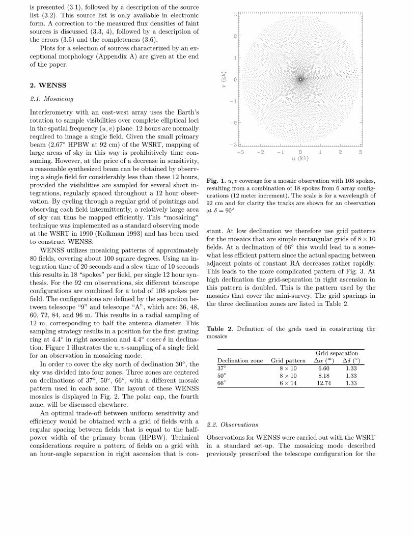
Interferometry with an east-west array uses the Earth’srotation to sample visibilities over complete elliptical lociin the spatial frequency (u, v) plane. 12 hours are normallyrequired to image a single field. Given the small primarybeam (2.67◦ HPBW at 92 cm) of the WSRT, mapping oflarge areas of sky in this way is prohibitively time con-suming. However, at the price of a decrease in sensitivity,a reasonable synthesized beam can be obtained by observ-ing a single field for considerably less than these 12 hours,provided the visibilities are sampled for several short in-tegrations, regularly spaced throughout a 12 hour obser-vation. By cycling through a regular grid of pointings andobserving each field intermittently, a relatively large areaof sky can thus be mapped efficiently. This “mosaicing”technique was implemented as a standard observing modeat the WSRT in 1990 (Kolkman 1993) and has been usedto construct WENSS.

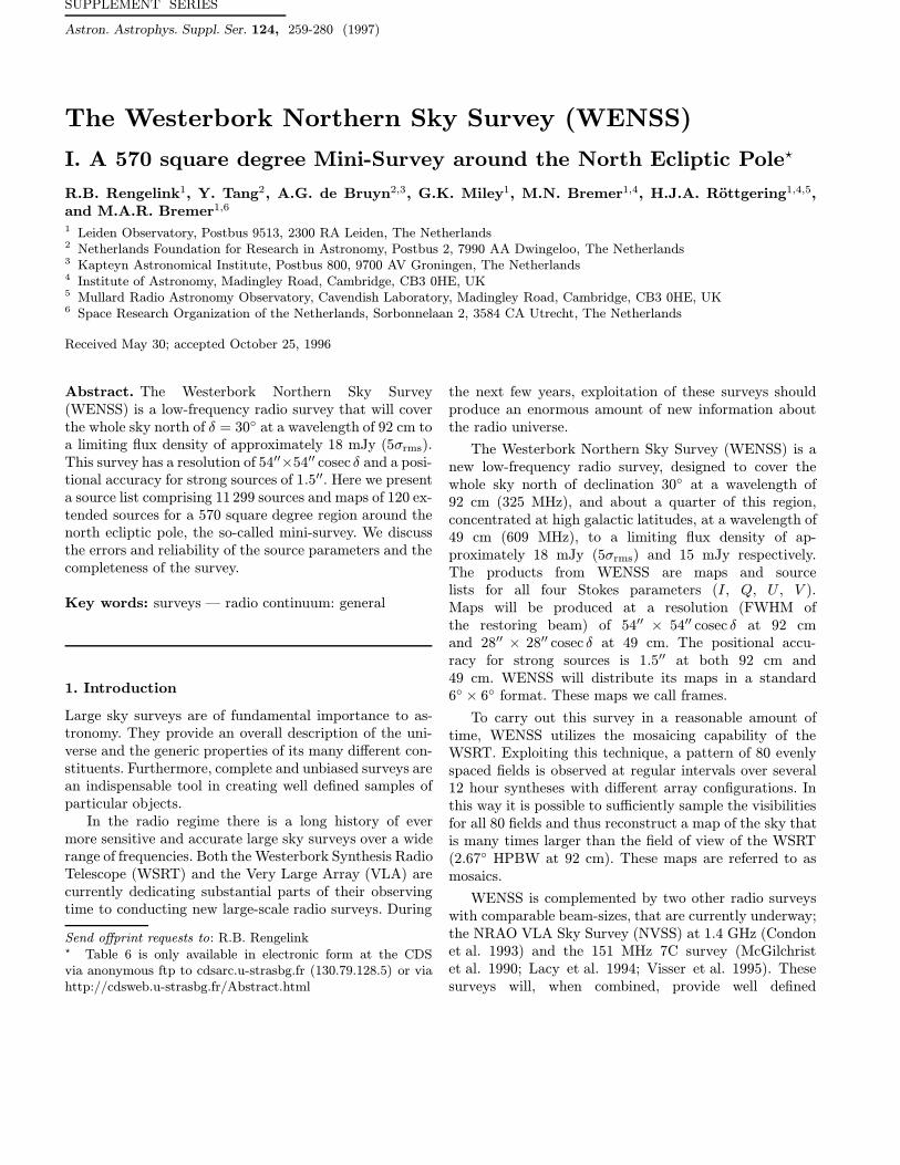
WENSS utilizes mosaicing patterns of approximately80 fields, covering about 100 square degrees. Using an in-tegration time of 20 seconds and a slew time of 10 secondsthis results in 18 “spokes” per field, per single 12 hour syn-thesis. For the 92 cm observations, six different telescopeconfigurations are combined for a total of 108 spokes perfield. The configurations are defined by the separation be-tween telescope “9” and telescope “A”, which are: 36, 48,60, 72, 84, and 96 m. This results in a radial sampling of12 m, corresponding to half the antenna diameter. Thissampling strategy results in a position for the first gratingring at 4.4◦ in right ascension and 4.4◦ cosec δ in declina-tion. Figure 1 illustrates the u, v-sampling of a single fieldfor an observation in mosaicing mode.

In order to cover the sky north of declination 30◦, thesky was divided into four zones. Three zones are centeredon declinations of 37◦, 50◦, 66◦, with a different mosaicpattern used in each zone. The layout of these WENSSmosaics is displayed in Fig. 2. The polar cap, the fourthzone, will be discussed elsewhere.

An optimal trade-off between uniform sensitivity andefficiency would be obtained with a grid of fields with aregular spacing between fields that is equal to the half-power width of the primary beam (HPBW). Technicalconsiderations require a pattern of fields on a grid withan hour-angle separation in right ascension that is con-

Fig. 1. u, v coverage for a mosaic observation with 108 spokes,resulting from a combination of 18 spokes from 6 array config-urations (12 meter increment). The scale is for a wavelength of92 cm and for clarity the tracks are shown for an observationat δ = 90◦

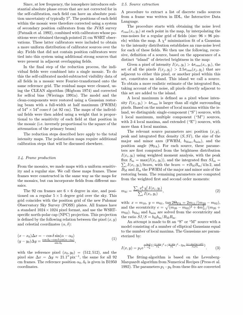
stant. At low declination we therefore use grid patternsfor the mosaics that are simple rectangular grids of 8× 10fields. At a declination of 66◦ this would lead to a some-what less efficient pattern since the actual spacing betweenadjacent points of constant RA decreases rather rapidly.This leads to the more complicated pattern of Fig. 3. Athigh declination the grid-separation in right ascension inthis pattern is doubled. This is the pattern used by themosaics that cover the mini-survey. The grid spacings inthe three declination zones are listed in Table 2.

Table 2. Definition of the grids used in constructing themosaics

Grid separationDeclination zone Grid pattern ∆α (m) ∆δ (◦)

37◦ 8× 10 6.60 1.3350◦ 8× 10 8.18 1.3366◦ 6× 14 12.74 1.33

2.2. Observations

Observations for WENSS were carried out with the WSRTin a standard set-up. The mosaicing mode describedpreviously prescribed the telescope configuration for the

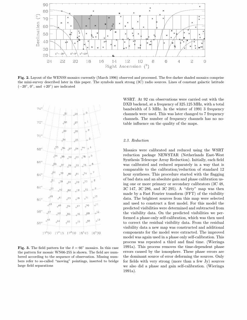
Fig. 2. Layout of the WENSS mosaics currently (March 1996) observed and processed. The five darker shaded mosaics comprisethe mini-survey described later in this paper. The symbols mark strong (3C) radio sources. Lines of constant galactic latitude(−20◦, 0◦, and +20◦) are indicated

Fig. 3. The field pattern for the δ = 66◦ mosaics. In this casethe pattern for mosaic WN66-255 is shown. The field are num-bered according to the sequence of observation. Missing num-bers refer to so-called “moving” pointings, inserted to bridgelarge field separations

WSRT. At 92 cm observations were carried out with theDXB backend, at a frequency of 325.125 MHz, with a totalbandwidth of 5 MHz. In the winter of 1991 3 frequencychannels were used. This was later changed to 7 frequencychannels. The number of frequency channels has no no-table influence on the quality of the maps.

2.3. Reduction

Mosaics were calibrated and reduced using the WSRTreduction package NEWSTAR (Netherlands East-WestSynthesis Telescope Array Reduction). Initially, each fieldwas calibrated and reduced separately in a way that iscomparable to the calibration/reduction of standard 12hour syntheses. This procedure started with the flaggingof bad data and an absolute gain and phase calibration us-ing one or more primary or secondary calibrators (3C 48,3C 147, 3C 286, and 3C 295). A “dirty” map was thenmade by a Fast Fourier transform (FFT) of the visibilitydata. The brightest sources from this map were selectedand used to construct a first model. For this model thepredicted visibilities were determined and subtracted fromthe visibility data. On the predicted visibilities we per-formed a phase-only self-calibration, which was then usedto correct the residual visibility data. From the residualvisibility data a new map was constructed and additionalcomponents for the model were extracted. The improvedmodel was again used in a phase only self-calibration. Thisprocess was repeated a third and final time. (Wieringa1991a). This process removes the time-dependent phaseerrors caused by the ionosphere. These phase errors arethe dominant source of error deforming the sources. Onlyfor fields with very strong (more than a few Jy) sourceswe also did a phase and gain self-calibration. (Wieringa1991a).

Since, at low frequency, the ionosphere introduces sub-stantial absolute phase errors that are not corrected for inthe self-calibration, each field can have an absolute posi-tion uncertainty of typically 5′′. The positions of each fieldwithin the mosaic were therefore corrected using a systemof secondary position calibrators from the JVAS survey(Patnaik et al. 1992), combined with calibrators whose po-sitions were obtained through pointed 21 cm WSRT obser-vations. These latter calibrators were included to obtaina more uniform distribution of calibrator sources over thesky. Fields that did not contain position calibrators weretied into this system using additional strong sources thatwere present in adjacent overlapping fields.

In the final step of the reduction process, the indi-vidual fields were combined into a single mosaic. To dothis the self-calibrated model-subtracted visibility data ofall fields in a mosaic were Fourier-transformed onto thesame reference grid. The residual maps were cleaned, us-ing the CLEAN algorithm (Hogbom 1974) and correctedfor selfcal bias (Wieringa 1991a). The model and theclean-components were restored using a Gaussian restor-ing beam with a full-width at half maximum (FWHM)of 54′′ × 54′′ cosec δ (at 92 cm). The maps of the individ-ual fields were then added using a weight that is propor-tional to the sensitivity of each field at that position inthe mosaic (i.e. inversely proportional to the square of theattenuation of the primary beam)

The reduction steps described here apply to the totalintensity maps. The polarization maps require additionalcalibration steps that will be discussed elsewhere.

2.4. Frame production

From the mosaics, we made maps with a uniform sensitiv-ity and a regular size. We call these maps frames. Theseframes were constructed in the same way as the maps forthe mosaics, but can incorporate fields from different mo-saics.

The 92 cm frames are 6 × 6 degree in size, and posi-tioned on a regular 5 × 5 degree grid over the sky. Thisgrid coincides with the position grid of the new PalomarObservatory Sky Survey (POSS) plates. All frames havea standard 1024× 1024 pixel format, and use the WSRT-specific north-polar cap (NPC) projection. This projectionis defined by the following relation between the pixel (x, y)and celestial coordinates (α, δ):

(x− x0)∆x = − cos δ sin(α− α0)

(y − y0)∆y = cos δ0−cos δ cos(α−α0)sin δ0

,(1)

with the reference pixel (x0, y0) = (512, 512), and thepixel size ∆x = ∆y ≈ 21.1′′ pix−1, the same for all 92cm frames. The reference position α0, δ0 is given in B1950coordinates.

2.5. Source extraction

A procedure to extract a list of discrete radio sourcesfrom a frame was written in IDL, the Interactive DataLanguage.

The procedure starts with obtaining the noise levelσrms(xi, yi) at each point in the map, by interpolating therms-noises for a regular grid of fields (size: 96 × 96 pix-els) within the map. A χ2 minimization fit of a Gaussianto the intensity distribution establishes an rms-noise levelfor each of these fields. We then use the following, recur-sive, definition of a source, based on the appearance of adistinct “island” of detected brightness in the map:

Given a pixel of intensity I(xi, yi) > 4σrms(xi, yi), theset of all the pixels I(xj , yj) > 2.5σrms(xj , yj) that areadjacent to either this pixel, or another pixel within thisset, constitutes an island. This island we call a source.To obtain a more realistic estimate of the integrated flux,taking account of the noise, all pixels directly adjacent tothis set are added to the island.

A local maximum is defined as a pixel whose inten-sity I(xi, yi) > 4σrms is larger than all eight surroundingpixels. Based on the number of local maxima within the is-land, we distinguish: single-component (“S”) sources, with1 local maximum, multiple component (“M”) sources,with 2-4 local maxima, and extended (“E”) sources, withmore than 4 local maxima.

The relevant source parameters are: position (x, y),peak and integrated flux density (S, SI), the size of themajor and minor axes (FWHM, bMax, bmin), and theposition angle (ΘPA). For each source, these parame-ters are first computed from the brightness distributionI(xi, yi) using weighted moment analysis, with the peakflux Sm = max(I(xi, yi)), and the integrated flux SIm =∑i I(xi, yi)/beam, with the beam = πBMBm/4 ln 2, and

BM andBm the FWHM of the major and minor axis of therestoring beam. The remaining parameters are computedfrom the weighted first and second order moments:

mkl =

∑i xki y

li I(xi, yi)∑

i I(xi, yi), (2)

with: x = m10, y = m01, tan 2ΘPA = 2m11/(m20 −m02),and the eccentricity e =

√(m20 −m02)2 + 4m2

11/(m20 +m02). bMaj and bmin are solved from the eccentricity andthe ratio SI/S = bMbm/BMBm.

An attempt is made to fit an “S” or “M” source with amodel consisting of a number of elliptical Gaussians equalto the number of local maxima. The Gaussians are param-eterized by:

I(x, y) = p1e− ln 2

1−p26

{(x−p2p4

)2+(y−p3p5

)2−2p6(x−p2)(y−p3)

p4p5}. (3)

The fitting-algorithm is based on the Levenberg-Marquardt algorithm from Numerical Recipes (Press et al.1992). The parameters p1−p6 from these fits are converted

Table 3. The 92 cm mosaics included in the mini-survey. Listed are the nominal mosaic center and the epochs of observationfor the different telescope configurations, defined by the distance between telescopes “9” and “A”

Mosaic Mosaic center (B1950) Epochs of observation (yymmdd)Right Ascension Declination 36 m 48 m 60 m 72 m 84 m 96 m

WN66 217 14h26m 66◦00′ 930201 930131 940416 930102 930128 930126

WN66 236 15h43m 66◦00′ 920112 920214 930109 911201 911215 911222WN66 255 16h59m 66◦00′ 910216 910223 910311 910114 910205 910208

WN66 274 18h16m 66◦00′ 910217 910224 910302 910120 910202 910209

WN66 293 19h32m 66◦00′ 910218 910225 910303 910329 910201 910210

Table 4. The high-resolution 92 cm frames included in themini-survey

Frame Map Center (B1950)RA Dec

WNH60 218 14h34m00s 60◦00′

WNH60 228 15h12m00s 60◦00′

WNH60 237 15h50m00s 60◦00′

WNH60 247 16h28m00s 60◦00′

WNH60 256 17h06m00s 60◦00′

WNH60 266 17h44m00s 60◦00′

WNH60 275 18h22m00s 60◦00′

WNH60 285 19h00m00s 60◦00′

WNH60 294 19h38m00s 60◦00′

WNH65 220 14h40m00s 65◦00′

WNH65 231 15h24m00s 65◦00′

WNH65 242 16h08m00s 65◦00′

WNH65 253 16h52m00s 65◦00′

WNH65 264 17h36m00s 65◦00′

WNH65 275 18h20m00s 65◦00′

WNH65 286 19h04m00s 65◦00′

WNH65 297 19h48m00s 65◦00′

WNH70 221 14h43m00s 70◦00′

WNH70 234 15h36m00s 70◦00′

WNH70 247 16h28m00s 70◦00′

WNH70 260 17h20m00s 70◦00′

WNH70 273 18h12m00s 70◦00′

WNH70 286 19h04m00s 70◦00′

WNH70 299 19h56m00s 70◦00′

to position, flux densities, major and minor axis and posi-tion angle and used to describe the source. If the algorithmfails to properly fit a source are the values from momentanalysis used to parameterize the source. The values frommoment analysis are also used for “E” sources. For “M”sources as a whole the position and morphology are es-tablished through moment analysis, while the peak fluxdensity is the maximum of the peak flux densities of thecomponents and the integrated flux density is the sum ofthe integrated flux densities of the components.

We find that the estimates of the flux densities and thesource morphology are affected by biases at low signal-to-

noise ratios. We therefore apply empirical corrections tothe flux-density estimates. These corrections are discussedin Sect. 3.4.

3. The mini-survey

The WENSS project initially concentrated on a relativelysmall area of sky roughly centered on the North EclipticPole. This region was chosen to coincide with the NEP-VLA survey at 1.5 GHz (Kollgaard et al. 1995), the deep7C North Ecliptic Cap survey (Lacy et al. 1995; Visseret al. 1995), and the deepest part of the ROSAT AllSky survey (Bohringer et al. 1991; Bower et al. 1996) andIRAS survey (Hacking & Houck 1987).

Our original intention was to base our complete anal-ysis of errors and reliability on the mini-survey region.However, data from various other parts of the surveyhave been included in this analysis. Nevertheless the mini-survey constitutes the most thoroughly analyzed part ofWENSS to date. Furthermore, data from the mini-surveyhas already been used extensively for various follow-up projects, including a search for gravitational lenses(CLASS, Myers et al. 1995; Snellen et al. 1995), and in-vestigations of samples of faint Gigaherz peaked spectrumsources and faint ultra steep spectrum sources.

3.1. Observations

Frames were constructed from the five mosaics listed inTable 3. The mosaics are labeled by the declination andapproximate right-ascension of their center. Four of mo-saics were observed at the start of the WENSS projectin the spring of 1991. Mosaic WN66 − 217 was later in-cluded in the mini-survey to improve the overlap with the7C survey (Visser et al. 1995). Figure 2 shows the layoutof these mosaics within the the survey.

A list of the 24 high resolution 92 cm frames includedin the mini-survey is presented in Table 4. The framesare labeled by the declination and approximate right-ascension of their center. Figure 4 shows the layout ofthese fields.

The theoretical noise level for WENSS is approxi-mately 2 mJy beam−1. Sidelobe confusion increases this

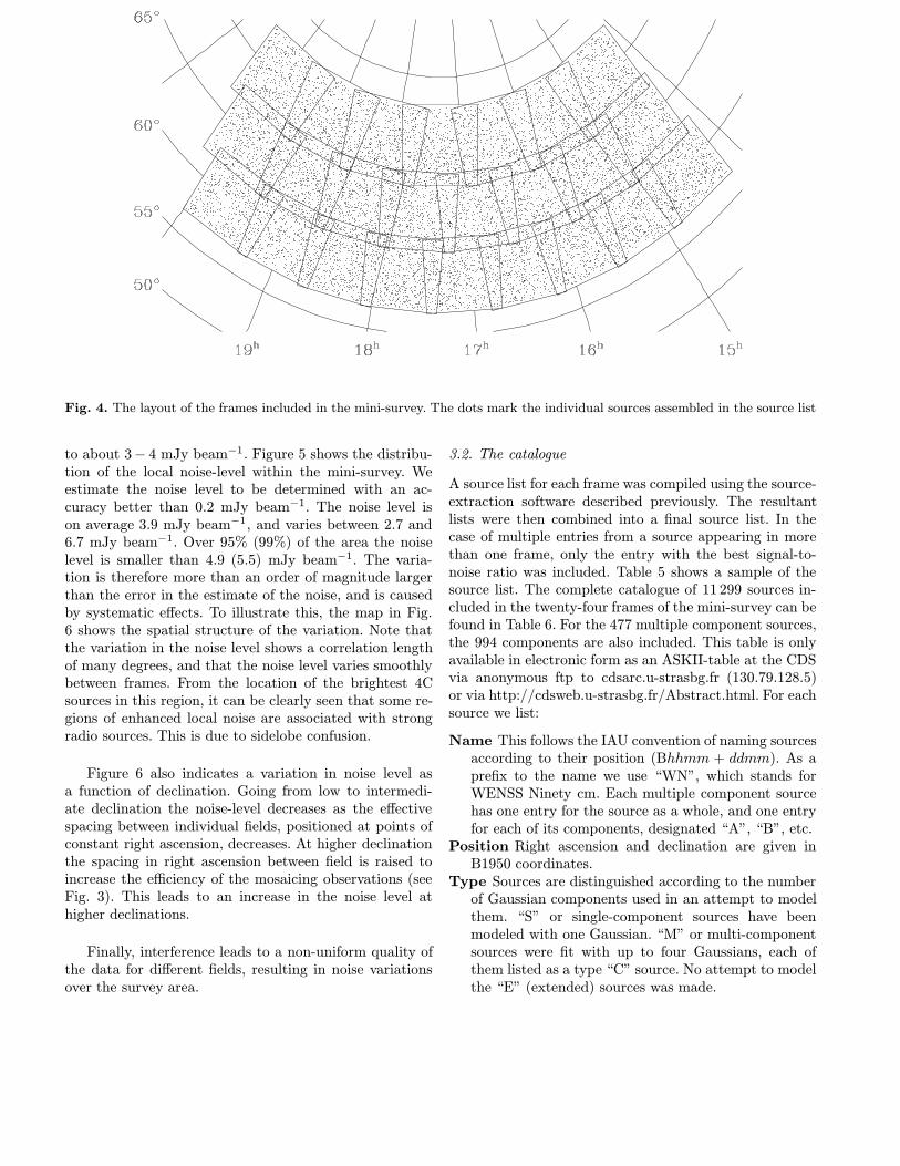
Fig. 4. The layout of the frames included in the mini-survey. The dots mark the individual sources assembled in the source list

to about 3− 4 mJy beam−1. Figure 5 shows the distribu-tion of the local noise-level within the mini-survey. Weestimate the noise level to be determined with an ac-curacy better than 0.2 mJy beam−1. The noise level ison average 3.9 mJy beam−1, and varies between 2.7 and6.7 mJy beam−1. Over 95% (99%) of the area the noiselevel is smaller than 4.9 (5.5) mJy beam−1. The varia-tion is therefore more than an order of magnitude largerthan the error in the estimate of the noise, and is causedby systematic effects. To illustrate this, the map in Fig.6 shows the spatial structure of the variation. Note thatthe variation in the noise level shows a correlation lengthof many degrees, and that the noise level varies smoothlybetween frames. From the location of the brightest 4Csources in this region, it can be clearly seen that some re-gions of enhanced local noise are associated with strongradio sources. This is due to sidelobe confusion.

Figure 6 also indicates a variation in noise level asa function of declination. Going from low to intermedi-ate declination the noise-level decreases as the effectivespacing between individual fields, positioned at points ofconstant right ascension, decreases. At higher declinationthe spacing in right ascension between field is raised toincrease the efficiency of the mosaicing observations (seeFig. 3). This leads to an increase in the noise level athigher declinations.

Finally, interference leads to a non-uniform quality ofthe data for different fields, resulting in noise variationsover the survey area.

3.2. The catalogue

A source list for each frame was compiled using the source-extraction software described previously. The resultantlists were then combined into a final source list. In thecase of multiple entries from a source appearing in morethan one frame, only the entry with the best signal-to-noise ratio was included. Table 5 shows a sample of thesource list. The complete catalogue of 11 299 sources in-cluded in the twenty-four frames of the mini-survey can befound in Table 6. For the 477 multiple component sources,the 994 components are also included. This table is onlyavailable in electronic form as an ASKII-table at the CDSvia anonymous ftp to cdsarc.u-strasbg.fr (130.79.128.5)or via http://cdsweb.u-strasbg.fr/Abstract.html. For eachsource we list:

Name This follows the IAU convention of naming sourcesaccording to their position (Bhhmm + ddmm). As aprefix to the name we use “WN”, which stands forWENSS Ninety cm. Each multiple component sourcehas one entry for the source as a whole, and one entryfor each of its components, designated “A”, “B”, etc.

Position Right ascension and declination are given inB1950 coordinates.

Type Sources are distinguished according to the numberof Gaussian components used in an attempt to modelthem. “S” or single-component sources have beenmodeled with one Gaussian. “M” or multi-componentsources were fit with up to four Gaussians, each ofthem listed as a type “C” source. No attempt to modelthe “E” (extended) sources was made.

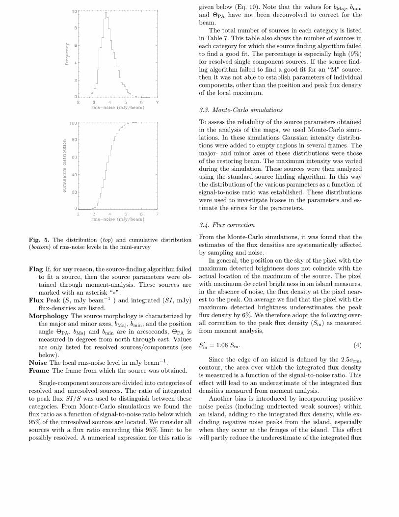
Fig. 5. The distribution (top) and cumulative distribution(bottom) of rms-noise levels in the mini-survey

Flag If, for any reason, the source-finding algorithm failedto fit a source, then the source parameters were ob-tained through moment-analysis. These sources aremarked with an asterisk “∗”.

Flux Peak (S, mJy beam−1 ) and integrated (SI, mJy)flux-densities are listed.

Morphology The source morphology is characterized bythe major and minor axes, bMaj, bmin, and the positionangle ΘPA. bMaj and bmin are in arcseconds, ΘPA ismeasured in degrees from north through east. Valuesare only listed for resolved sources/components (seebelow).

Noise The local rms-noise level in mJy beam−1.Frame The frame from which the source was obtained.

Single-component sources are divided into categories ofresolved and unresolved sources. The ratio of integratedto peak flux SI/S was used to distinguish between thesecategories. From Monte-Carlo simulations we found theflux ratio as a function of signal-to-noise ratio below which95% of the unresolved sources are located. We consider allsources with a flux ratio exceeding this 95% limit to bepossibly resolved. A numerical expression for this ratio is

given below (Eq. 10). Note that the values for bMaj, bmin

and ΘPA have not been deconvolved to correct for thebeam.

The total number of sources in each category is listedin Table 7. This table also shows the number of sources ineach category for which the source finding algorithm failedto find a good fit. The percentage is especially high (9%)for resolved single component sources. If the source find-ing algorithm failed to find a good fit for an “M” source,then it was not able to establish parameters of individualcomponents, other than the position and peak flux densityof the local maximum.

3.3. Monte-Carlo simulations

To assess the reliability of the source parameters obtainedin the analysis of the maps, we used Monte-Carlo simu-lations. In these simulations Gaussian intensity distribu-tions were added to empty regions in several frames. Themajor- and minor axes of these distributions were thoseof the restoring beam. The maximum intensity was variedduring the simulation. These sources were then analyzedusing the standard source finding algorithm. In this waythe distributions of the various parameters as a function ofsignal-to-noise ratio was established. These distributionswere used to investigate biases in the parameters and es-timate the errors for the parameters.

3.4. Flux correction

From the Monte-Carlo simulations, it was found that theestimates of the flux densities are systematically affectedby sampling and noise.

In general, the position on the sky of the pixel with themaximum detected brightness does not coincide with theactual location of the maximum of the source. The pixelwith maximum detected brightness in an island measures,in the absence of noise, the flux density at the pixel near-est to the peak. On average we find that the pixel with themaximum detected brightness underestimates the peakflux density by 6%. We therefore adopt the following over-all correction to the peak flux density (Sm) as measuredfrom moment analysis,

S′m = 1.06 Sm. (4)

Since the edge of an island is defined by the 2.5σrms

contour, the area over which the integrated flux densityis measured is a function of the signal-to-noise ratio. Thiseffect will lead to an underestimate of the integrated fluxdensities measured from moment analysis.

Another bias is introduced by incorporating positivenoise peaks (including undetected weak sources) withinan island, adding to the integrated flux density, while ex-cluding negative noise peaks from the island, especiallywhen they occur at the fringes of the island. This effectwill partly reduce the underestimate of the integrated flux

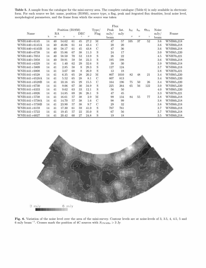
Table 5. A sample from the catalogue for the mini-survey area. The complete catalogue (Table 6) is only available in electronicform. For each source we list: name, position (B1950), source type, a flag, peak and itegrated flux densities, local noise level,morphological parameters, and the frame from which the source was taken

FluxPosition (B1950) Type/ Peak Int. bM bm ΘPA Noise

Name RA DEC Flag mJy/ mJy mJy/ Frameh m s ◦ ′ ′′ beam ′′ ′′ ◦ beam

WNB1440+6145 14 40 54.62 61 45 27.2 M 47 57 105 37 52 3.6 WNH60 218WNB1440+6145A 14 40 46.06 61 44 43.4 C 20 20 3.6 WNH60 218WNB1440+6145B 14 40 58.17 61 45 43.8 C 47 36 3.6 WNH60 218WNB1440+6738 14 40 55.86 67 38 11.3 S 24 17 3.0 WNH65 220WNB1440+7053 14 40 58.50 70 53 13.9 S 26 22 4.5 WNH70 221WNB1440+5958 14 40 59.91 59 58 22.3 S 195 198 3.6 WNH60 218WNB1441+6229 14 41 1.40 62 29 32.6 S 39 30 3.9 WNH60 218WNB1441+5809 14 41 2.85 58 9 29.3 S 127 124 3.7 WNH60 218WNB1441+6808 14 41 3.67 68 8 26.9 S 12 18 2.8 WNH70 221WNB1441+6528 14 41 6.35 65 28 20.2 M 807 1010 82 48 21 3.4 WNH65 220WNB1441+6528A 14 41 5.52 65 28 8.1 C 807 813 3.4 WNH65 220WNB1441+6528B 14 41 10.16 65 29 15.5 C 164 196 75 50 26 3.4 WNH65 220WNB1441+6730 14 41 9.06 67 30 34.9 S 225 264 65 56 122 3.0 WNH65 220WNB1441+6333 14 41 9.62 63 33 12.1 S 56 50 4.0 WNH65 220WNB1441+6926 14 41 14.85 69 26 26.1 S 47 45 3.3 WNH70 221WNB1441+5738 14 41 16.61 57 38 2.9 M 99 134 84 55 77 3.8 WNH60 218WNB1441+5738A 14 41 14.70 57 38 1.6 C 98 99 3.8 WNH60 218WNB1441+5738B 14 41 23.90 57 38 9.7 C 29 32 3.8 WNH60 218WNB1441+6159 14 41 17.30 61 59 41.0 S 767 761 3.7 WNH60 218WNB1441+5722 14 41 19.45 57 22 35.0 S 67 56 3.7 WNH60 218WNB1441+6027 14 41 20.42 60 27 24.8 S 19 18 3.5 WNH60 218

Fig. 6. Variation of the noise level over the area of the mini-survey. Contour levels are at noise-levels of 3, 3.5, 4, 4.5, 5 and6 mJy beam−1. Crosses mark the position of 4C sources with S178 MHz > 3 Jy

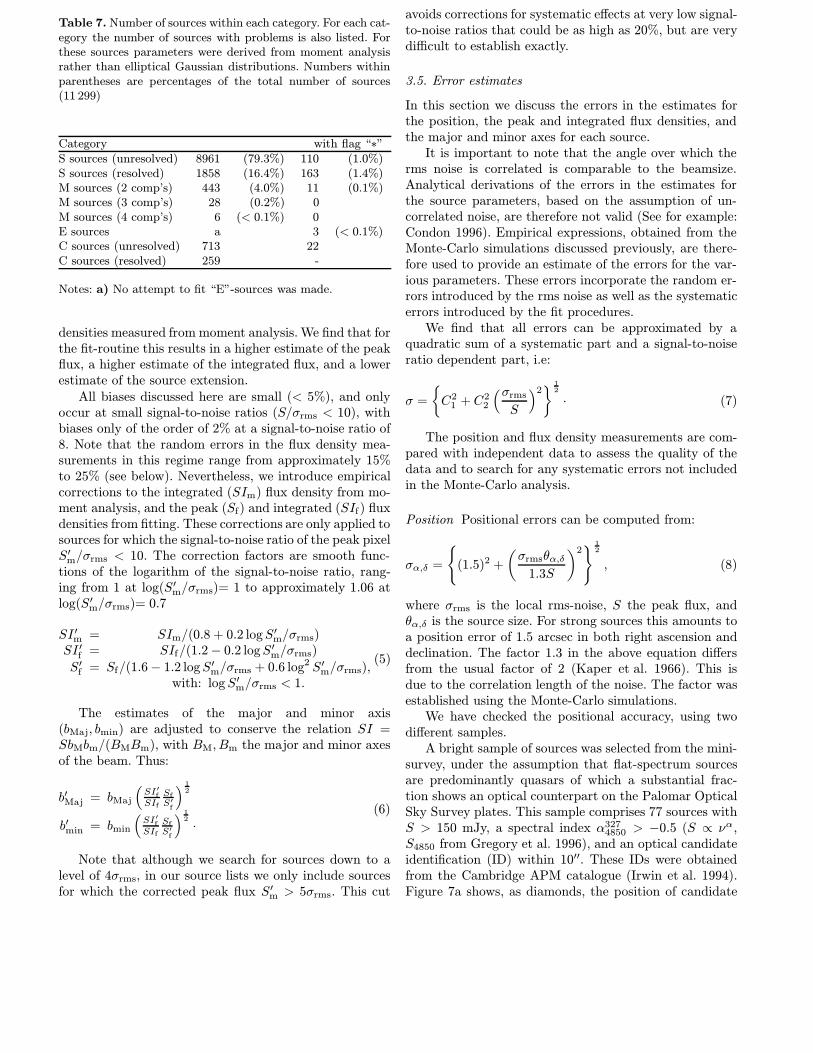
Table 7. Number of sources within each category. For each cat-egory the number of sources with problems is also listed. Forthese sources parameters were derived from moment analysisrather than elliptical Gaussian distributions. Numbers withinparentheses are percentages of the total number of sources(11 299)

Category with flag “∗”S sources (unresolved) 8961 (79.3%) 110 (1.0%)S sources (resolved) 1858 (16.4%) 163 (1.4%)M sources (2 comp’s) 443 (4.0%) 11 (0.1%)M sources (3 comp’s) 28 (0.2%) 0M sources (4 comp’s) 6 (< 0.1%) 0E sources a 3 (< 0.1%)C sources (unresolved) 713 22C sources (resolved) 259 -

Notes: a) No attempt to fit “E”-sources was made.

densities measured from moment analysis. We find that forthe fit-routine this results in a higher estimate of the peakflux, a higher estimate of the integrated flux, and a lowerestimate of the source extension.

All biases discussed here are small (< 5%), and onlyoccur at small signal-to-noise ratios (S/σrms < 10), withbiases only of the order of 2% at a signal-to-noise ratio of8. Note that the random errors in the flux density mea-surements in this regime range from approximately 15%to 25% (see below). Nevertheless, we introduce empiricalcorrections to the integrated (SIm) flux density from mo-ment analysis, and the peak (Sf) and integrated (SIf) fluxdensities from fitting. These corrections are only applied tosources for which the signal-to-noise ratio of the peak pixelS′m/σrms < 10. The correction factors are smooth func-tions of the logarithm of the signal-to-noise ratio, rang-ing from 1 at log(S′m/σrms)= 1 to approximately 1.06 atlog(S′m/σrms)= 0.7

SI ′m = SIm/(0.8 + 0.2 logS′m/σrms)SI ′f = SIf/(1.2− 0.2 logS′m/σrms)

S′f = Sf/(1.6− 1.2 logS′m/σrms + 0.6 log2 S′m/σrms),with: logS′m/σrms < 1.

(5)

The estimates of the major and minor axis(bMaj, bmin) are adjusted to conserve the relation SI =SbMbm/(BMBm), with BM, Bm the major and minor axesof the beam. Thus:

b′Maj = bMaj

(SI′fSIf

Sf

S′f

) 12

b′min = bmin

(SI′fSIf

Sf

S′f

) 12

·(6)

Note that although we search for sources down to alevel of 4σrms, in our source lists we only include sourcesfor which the corrected peak flux S′m > 5σrms. This cut

avoids corrections for systematic effects at very low signal-to-noise ratios that could be as high as 20%, but are verydifficult to establish exactly.

3.5. Error estimates

In this section we discuss the errors in the estimates forthe position, the peak and integrated flux densities, andthe major and minor axes for each source.

It is important to note that the angle over which therms noise is correlated is comparable to the beamsize.Analytical derivations of the errors in the estimates forthe source parameters, based on the assumption of un-correlated noise, are therefore not valid (See for example:Condon 1996). Empirical expressions, obtained from theMonte-Carlo simulations discussed previously, are there-fore used to provide an estimate of the errors for the var-ious parameters. These errors incorporate the random er-rors introduced by the rms noise as well as the systematicerrors introduced by the fit procedures.

We find that all errors can be approximated by aquadratic sum of a systematic part and a signal-to-noiseratio dependent part, i.e:

σ =

{C2

1 + C22

(σrms

S

)2} 1

2

· (7)

The position and flux density measurements are com-pared with independent data to assess the quality of thedata and to search for any systematic errors not includedin the Monte-Carlo analysis.

Position Positional errors can be computed from:

σα,δ =

{(1.5)2 +

(σrmsθα,δ

1.3S

)2} 1

2

, (8)

where σrms is the local rms-noise, S the peak flux, andθα,δ is the source size. For strong sources this amounts toa position error of 1.5 arcsec in both right ascension anddeclination. The factor 1.3 in the above equation differsfrom the usual factor of 2 (Kaper et al. 1966). This isdue to the correlation length of the noise. The factor wasestablished using the Monte-Carlo simulations.

We have checked the positional accuracy, using twodifferent samples.

A bright sample of sources was selected from the mini-survey, under the assumption that flat-spectrum sourcesare predominantly quasars of which a substantial frac-tion shows an optical counterpart on the Palomar OpticalSky Survey plates. This sample comprises 77 sources withS > 150 mJy, a spectral index α327

4850 > −0.5 (S ∝ να,S4850 from Gregory et al. 1996), and an optical candidateidentification (ID) within 10′′. These IDs were obtainedfrom the Cambridge APM catalogue (Irwin et al. 1994).Figure 7a shows, as diamonds, the position of candidate

Fig. 7. a) Normalized position difference for candidate optical IDs of flat spectrum radio sources (diamonds) and for VLApositions (crosses). The concentric circles mark the 1, 2, and 3σ position differences respectively. b-c) The distribution ofnormalized position differences in right ascension and declination. Overlayed are the expected Gaussian distributions

IDs with respect to the radio position, normalized by theestimate of the errors in α and δ. The errors were com-puted by adding the errors from Eq. (8) in quadrature toa positional error of 1′′ for the optical ID.

A faint sample was obtained from preliminary re-sults of the CLASS gravitational lens survey (Myers et al.1995). As part of this survey a large number of faint(S < 200 mJy), flat-spectrum (α > −0.5) WENSS sourceswas mapped using the VLA at 8.5 GHz in A-array, tosearch for a characteristic gravitational lens morphology.Accurate (σ < 1′′) positions for these sources were ob-tained as a by-product. Figure 7a shows, as crosses, theVLA positions, with respect to the WENSS positions, nor-malized by the errors in right ascension and declination.

Figures 7b, c show the combined distribution of po-sition differences of both samples. These figures indicatethat the error estimates are probably conservative in thesense that they overestimate the variance in the positiondifference. However, this overestimate allows for some pos-sible systematic offsets at the 0.5′′ level, as indicated bythe skew distribution in right ascension.

Flux densities The relative errors in the flux densities, canbe computed from:

σS

S=

{C2

1 + C22

(σrms

S

)2} 1

2

, (9)

with S/σrms the signal-to-noise ratio. The values for theconstants depend on the parameter being measured, andcan be read from the following Table 8.

The constant C2 was estimated from Monte-Carlo sim-ulations for unresolved sources. A conservative estimatefor C1 includes a 3% upper limit to the accuracy of the re-duction process and source-finding algorithm and a < 2%variation in the flux calibration for different mosaics. Forthe peak flux we add 5% to the error for the estimate

Table 8. Numerical values for the constants C1 and C2 inEq. (9), determining the errors in the flux density estimates

Flux density (method) (S) C1 C2

Peak (moment) (Sm) 0.06 1.0Integr. (moment) (SIm) 0.04 1.7Peak (fit) (Sf) 0.04 1.3Integr. (fit) (SIf) 0.04 1.3

made through moment analysis to take into account theadditional uncertainty due to sampling.

These errors do not include systematic errors intro-duced in the data recording and data reduction. An es-timate of these errors can be obtained by a comparisonwith results from a standard observation at 92 cm withthe WSRT. For this we used a deep (6× 12h) observationcarried out by one of us (G de Bruyn) of a field that is notpart of the mini-survey and compared this with WENSSdata already available for this field. Figure 8 shows theratio of integrated flux densities as measured by WENSSand the standard WSRT observation. This figure indicatesthat there are no systematic errors. The figure also showsthat the error estimates are reasonable.

Extendedness An estimate of the extendedness of a sourcecan be obtained from the ratio of the integrated flux tothe peak flux SI/S = bMbm/(BMBm). However, a directapplication of Eq. (9) to establish the significance of aresult SI/S > 1 is only possible if the errors σSI andσS are independent. This is not the case. Rather, SI/Sshows a very skew distribution, with a tail toward highflux ratios, especially at low signal-to-noise ratios. Themedian of this distribution is found to be less than 1.

To establish a criterion for extendedness, we have de-termined the upper envelopes of the distribution of SI/S,

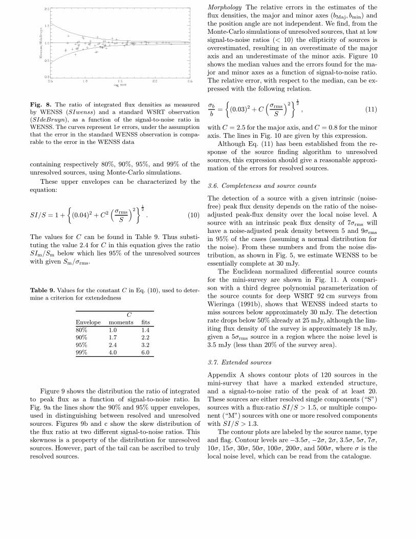
Fig. 8. The ratio of integrated flux densities as measuredby WENSS (SIwenss) and a standard WSRT observation(SIdeBruyn), as a function of the signal-to-noise ratio inWENSS. The curves represent 1σ errors, under the assumptionthat the error in the standard WENSS observation is compa-rable to the error in the WENSS data

containing respectively 80%, 90%, 95%, and 99% of theunresolved sources, using Monte-Carlo simulations.

These upper envelopes can be characterized by theequation:

SI/S = 1 +

{(0.04)2 + C2

(σrms

S

)2} 1

2

. (10)

The values for C can be found in Table 9. Thus substi-tuting the value 2.4 for C in this equation gives the ratioSIm/Sm below which lies 95% of the unresolved sourceswith given Sm/σrms.

Table 9. Values for the constant C in Eq. (10), used to deter-mine a criterion for extendedness

C

Envelope moments fits

80% 1.0 1.490% 1.7 2.295% 2.4 3.299% 4.0 6.0

Figure 9 shows the distribution the ratio of integratedto peak flux as a function of signal-to-noise ratio. InFig. 9a the lines show the 90% and 95% upper envelopes,used in distinguishing between resolved and unresolvedsources. Figures 9b and c show the skew distribution ofthe flux ratio at two different signal-to-noise ratios. Thisskewness is a property of the distribution for unresolvedsources. However, part of the tail can be ascribed to trulyresolved sources.

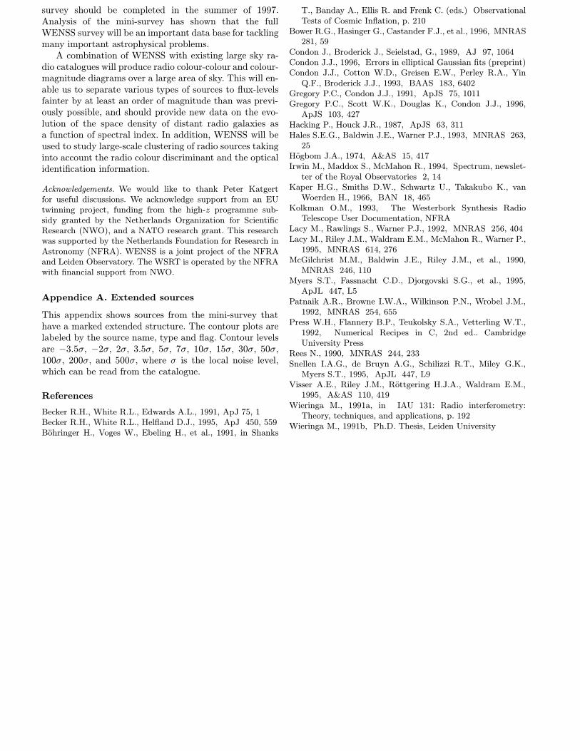
Morphology The relative errors in the estimates of theflux densities, the major and minor axes (bMaj, bmin) andthe position angle are not independent. We find, from theMonte-Carlo simulations of unresolved sources, that at lowsignal-to-noise ratios (< 10) the ellipticity of sources isoverestimated, resulting in an overestimate of the majoraxis and an underestimate of the minor axis. Figure 10shows the median values and the errors found for the ma-jor and minor axes as a function of signal-to-noise ratio.The relative error, with respect to the median, can be ex-pressed with the following relation.

σb

b=

{(0.03)2 + C

(σrms

S

)2} 1

2

, (11)

with C = 2.5 for the major axis, and C = 0.8 for the minoraxis. The lines in Fig. 10 are given by this expression.

Although Eq. (11) has been established from the re-sponse of the source finding algorithm to unresolvedsources, this expression should give a reasonable approxi-mation of the errors for resolved sources.

3.6. Completeness and source counts

The detection of a source with a given intrinsic (noise-free) peak flux density depends on the ratio of the noise-adjusted peak-flux density over the local noise level. Asource with an intrinsic peak flux density of 7σrms willhave a noise-adjusted peak density between 5 and 9σrms

in 95% of the cases (assuming a normal distribution forthe noise). From these numbers and from the noise dis-tribution, as shown in Fig. 5, we estimate WENSS to beessentially complete at 30 mJy.

The Euclidean normalized differential source countsfor the mini-survey are shown in Fig. 11. A compari-son with a third degree polynomial parameterization ofthe source counts for deep WSRT 92 cm surveys fromWieringa (1991b), shows that WENSS indeed starts tomiss sources below approximately 30 mJy. The detectionrate drops below 50% already at 25 mJy, although the lim-iting flux density of the survey is approximately 18 mJy,given a 5σrms source in a region where the noise level is3.5 mJy (less than 20% of the survey area).

3.7. Extended sources

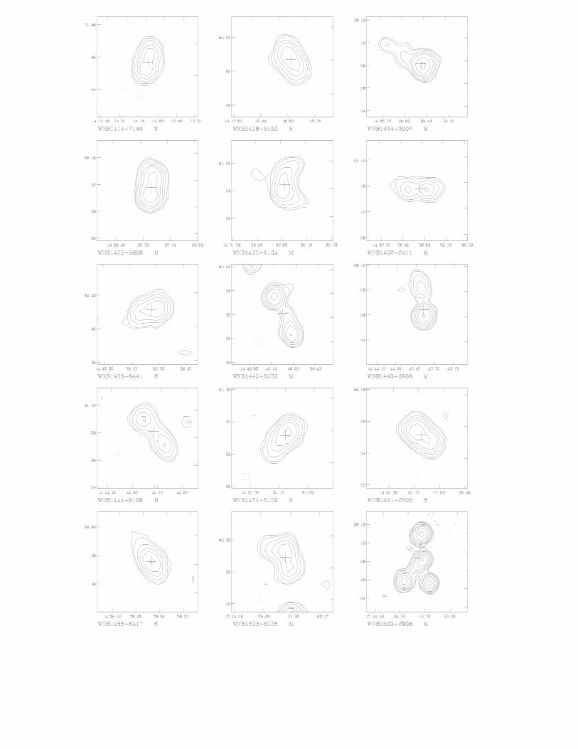
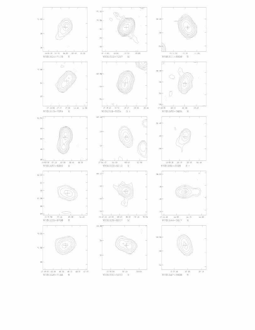
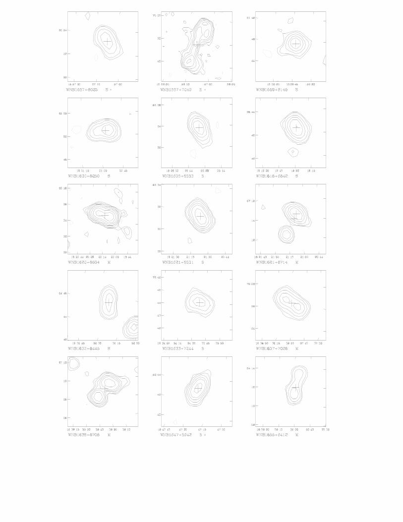
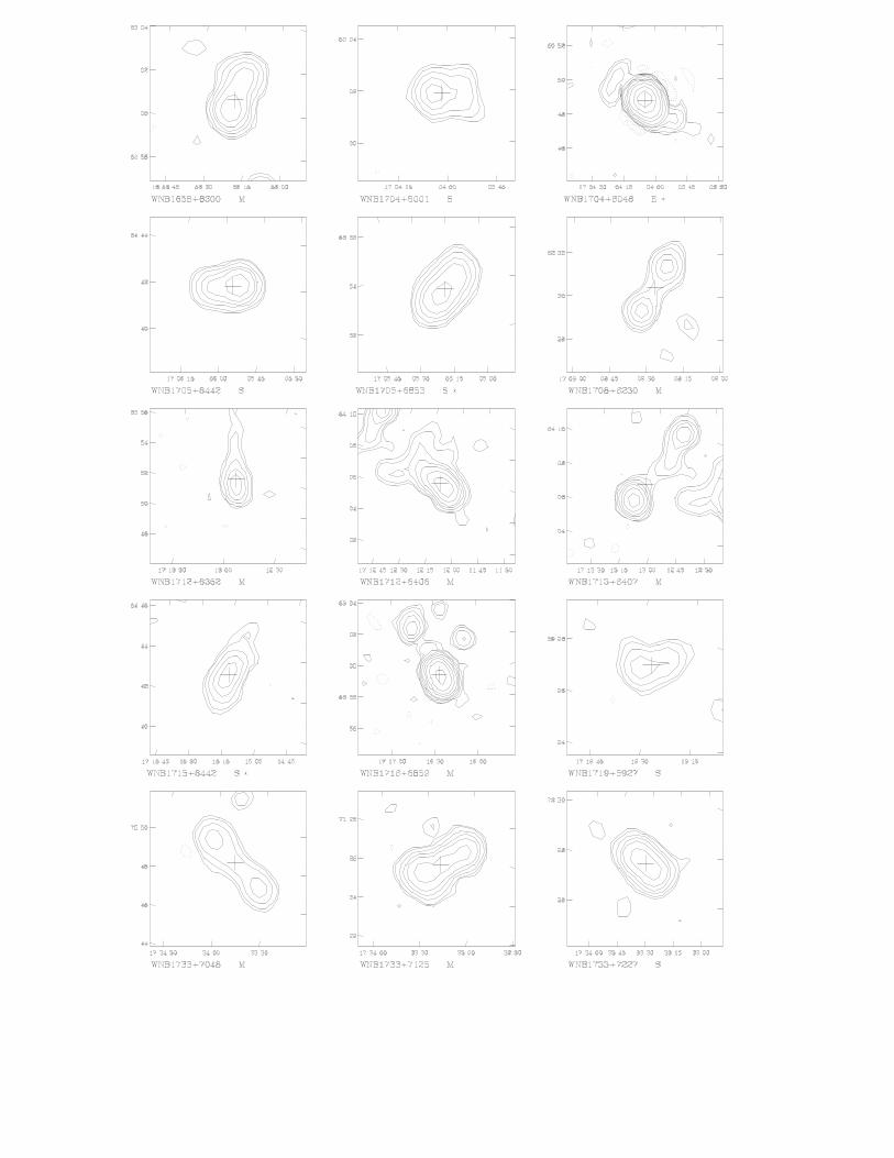
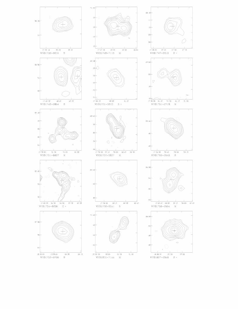
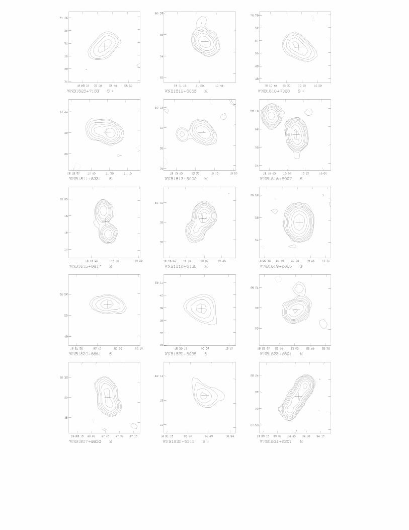
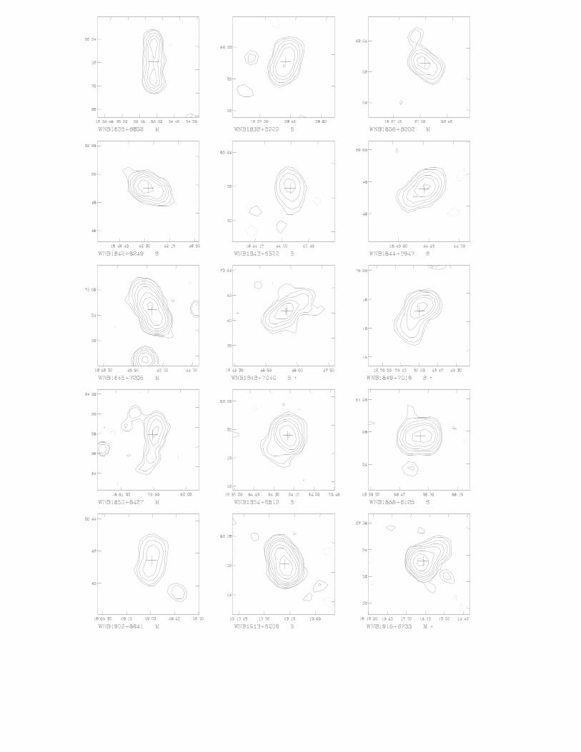
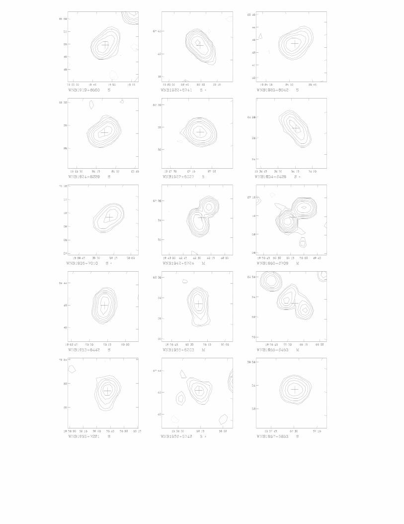
Appendix A shows contour plots of 120 sources in themini-survey that have a marked extended structure,and a signal-to-noise ratio of the peak of at least 20.These sources are either resolved single components (“S”)sources with a flux-ratio SI/S > 1.5, or multiple compo-nent (“M”) sources with one or more resolved componentswith SI/S > 1.3.

The contour plots are labeled by the source name, typeand flag. Contour levels are −3.5σ, −2σ, 2σ, 3.5σ, 5σ, 7σ,10σ, 15σ, 30σ, 50σ, 100σ, 200σ, and 500σ, where σ is thelocal noise level, which can be read from the catalogue.

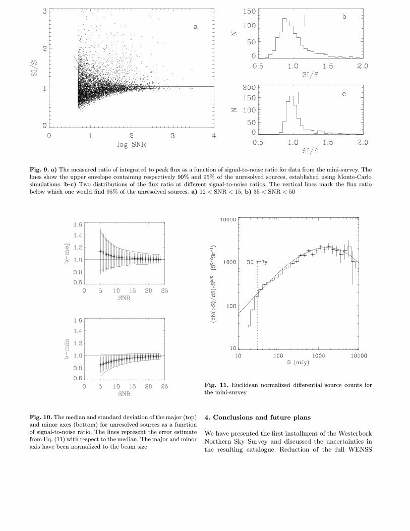
Fig. 9. a) The measured ratio of integrated to peak flux as a function of signal-to-noise ratio for data from the mini-survey. Thelines show the upper envelope containing respectively 90% and 95% of the unresolved sources, established using Monte-Carlosimulations. b-c) Two distributions of the flux ratio at different signal-to-noise ratios. The vertical lines mark the flux ratiobelow which one would find 95% of the unresolved sources. a) 12 < SNR < 15, b) 35 < SNR < 50

Fig. 10. The median and standard deviation of the major (top)and minor axes (bottom) for unresolved sources as a functionof signal-to-noise ratio. The lines represent the error estimatefrom Eq. (11) with respect to the median. The major and minoraxis have been normalized to the beam size

Fig. 11. Euclidean normalized differential source counts forthe mini-survey

4. Conclusions and future plans

We have presented the first installment of the WesterborkNorthern Sky Survey and discussed the uncertainties inthe resulting catalogue. Reduction of the full WENSS

survey should be completed in the summer of 1997.Analysis of the mini-survey has shown that the fullWENSS survey will be an important data base for tacklingmany important astrophysical problems.

A combination of WENSS with existing large sky ra-dio catalogues will produce radio colour-colour and colour-magnitude diagrams over a large area of sky. This will en-able us to separate various types of sources to flux-levelsfainter by at least an order of magnitude than was previ-ously possible, and should provide new data on the evo-lution of the space density of distant radio galaxies asa function of spectral index. In addition, WENSS will beused to study large-scale clustering of radio sources takinginto account the radio colour discriminant and the opticalidentification information.

Acknowledgements. We would like to thank Peter Katgertfor useful discussions. We acknowledge support from an EUtwinning project, funding from the high-z programme sub-sidy granted by the Netherlands Organization for ScientificResearch (NWO), and a NATO research grant. This researchwas supported by the Netherlands Foundation for Research inAstronomy (NFRA). WENSS is a joint project of the NFRAand Leiden Observatory. The WSRT is operated by the NFRAwith financial support from NWO.

Appendice A. Extended sources

This appendix shows sources from the mini-survey thathave a marked extended structure. The contour plots arelabeled by the source name, type and flag. Contour levelsare −3.5σ, −2σ, 2σ, 3.5σ, 5σ, 7σ, 10σ, 15σ, 30σ, 50σ,100σ, 200σ, and 500σ, where σ is the local noise level,which can be read from the catalogue.

References

Becker R.H., White R.L., Edwards A.L., 1991, ApJ 75, 1Becker R.H., White R.L., Helfland D.J., 1995, ApJ 450, 559Bohringer H., Voges W., Ebeling H., et al., 1991, in Shanks

T., Banday A., Ellis R. and Frenk C. (eds.) ObservationalTests of Cosmic Inflation, p. 210

Bower R.G., Hasinger G., Castander F.J., et al., 1996, MNRAS281, 59

Condon J., Broderick J., Seielstad, G., 1989, AJ 97, 1064Condon J.J., 1996, Errors in elliptical Gaussian fits (preprint)Condon J.J., Cotton W.D., Greisen E.W., Perley R.A., Yin

Q.F., Broderick J.J., 1993, BAAS 183, 6402Gregory P.C., Condon J.J., 1991, ApJS 75, 1011Gregory P.C., Scott W.K., Douglas K., Condon J.J., 1996,

ApJS 103, 427Hacking P., Houck J.R., 1987, ApJS 63, 311Hales S.E.G., Baldwin J.E., Warner P.J., 1993, MNRAS 263,

25Hogbom J.A., 1974, A&AS 15, 417Irwin M., Maddox S., McMahon R., 1994, Spectrum, newslet-

ter of the Royal Observatories 2, 14Kaper H.G., Smiths D.W., Schwartz U., Takakubo K., van

Woerden H., 1966, BAN 18, 465Kolkman O.M., 1993, The Westerbork Synthesis Radio

Telescope User Documentation, NFRALacy M., Rawlings S., Warner P.J., 1992, MNRAS 256, 404Lacy M., Riley J.M., Waldram E.M., McMahon R., Warner P.,

1995, MNRAS 614, 276McGilchrist M.M., Baldwin J.E., Riley J.M., et al., 1990,

MNRAS 246, 110Myers S.T., Fassnacht C.D., Djorgovski S.G., et al., 1995,

ApJL 447, L5Patnaik A.R., Browne I.W.A., Wilkinson P.N., Wrobel J.M.,

1992, MNRAS 254, 655Press W.H., Flannery B.P., Teukolsky S.A., Vetterling W.T.,

1992, Numerical Recipes in C, 2nd ed.. CambridgeUniversity Press

Rees N., 1990, MNRAS 244, 233Snellen I.A.G., de Bruyn A.G., Schilizzi R.T., Miley G.K.,

Myers S.T., 1995, ApJL 447, L9Visser A.E., Riley J.M., Rottgering H.J.A., Waldram E.M.,

1995, A&AS 110, 419Wieringa M., 1991a, in IAU 131: Radio interferometry:

Theory, techniques, and applications, p. 192Wieringa M., 1991b, Ph.D. Thesis, Leiden University