The Welfare Cost of Asymmetric Information:

Evidence from the U.K. Annuity Market∗

Liran EinavStanford and NBER

Amy FinkelsteinMIT and NBER

Paul SchrimpfMIT

November 7, 2006Preliminary and incomplete. Comments are very welcome.

Abstract

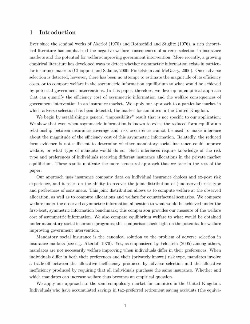
We estimate the welfare costs of asymmetric information within the U.K. annuity market.We first show theoretically that reduced form evidence of how “adversely selected” the marketis is not informative about the magnitude of these costs. This motivates our development andestimation of a structural model of the annuity contract choice. The model allows for privateinformation about risk type (mortality) as well as heterogeneity in preferences over differentcontract options. We focus on the choice of length of guarantee among individuals who arerequired to buy annuities. The results suggest that asymmetric information along the guaranteemargin reduces welfare relative to a first-best, symmetric information benchmark by about£145 million per year, or about 2.5 percent of annual premiums. We also find that governmentmandates, the canoncial solution to adverse selection problems, do not necessarily improve on

the asymmetric information equilibrium. Depending on the contract mandated, mandates couldreduce welfare by as much as £110 million annually, or increase it by as much as £145 millionannually. Since determining which mandates would be welfare improving is empirically difficult,our findings suggest that achieving welfare gains through mandatory social insurance may beharder in practice than simple theory would suggest.

JEL classification numbers: C13, C51, D14, D60, D82.Keywords: Annuities, contract choice, adverse selection, strutural estimation.

∗We are grateful to Jeff Brown, Peter Diamond, Wojciech Koczuk, Ben Olken, Casey Rothschild, and participants

at the MIT Industrial Organization Lunch, MIT Public Finance Lunch, and the Hoover Economics Bag Lunch

Seminar for helpful comments, to the National Institute of Aging for research support, and to several patient and

helpful employees at the firm whose data we analyze. Einav: leinav@stanford.edu; Finkelstein: afink@mit.edu;

Schrimpf: paul_s@mit.edu

1 Introduction

Ever since the seminal works of Akerlof (1970) and Rothschild and Stiglitz (1976), a rich theoret-

ical literature has emphasized the negative welfare consequences of adverse selection in insurance

markets and the potential for welfare-improving government intervention. More recently, a growing

empirical literature has developed ways to detect whether asymmetric information exists in particu-

lar insurance markets (Chiappori and Salanie, 2000; Finkelstein and McGarry, 2006). Once adverse

selection is detected, however, there has been no attempt to estimate the magnitude of its efficiency

costs, or to compare welfare in the asymmetric information equilibrium to what would be achieved

by potential government interventions. In this paper, therefore, we develop an empirical approach

that can quantify the efficiency cost of asymmetric information and the welfare consequences of

government intervention in an insurance market. We apply our approach to a particular market in

which adverse selection has been detected, the market for annuities in the United Kingdom.

We begin by establishing a general “impossibility” result that is not specific to our application.

We show that even when asymmetric information is known to exist, the reduced form equilibrium

relationship between insurance coverage and risk occurrence cannot be used to make inference

about the magnitude of the efficiency cost of this asymmetric information. Relatedly, the reduced

form evidence is not sufficient to determine whether mandatory social insurance could improve

welfare, or what type of mandate would do so. Such inferences require knowledge of the risk

type and preferences of individuals receiving different insurance allocations in the private market

equilibrium. These results motivate the more structural approach that we take in the rest of the

paper.

Our approach uses insurance company data on individual insurance choices and ex-post risk

experience, and it relies on the ability to recover the joint distribution of (unobserved) risk type

and preferences of consumers. This joint distribution allows us to compute welfare at the observed

allocation, as well as to compute allocations and welfare for counterfactual scenarios. We compare

welfare under the observed asymmetric information allocation to what would be achieved under the

first-best, symmetric information benchmark; this comparison provides our measure of the welfare

cost of asymmetric information. We also compare equilibrium welfare to what would be obtained

under mandatory social insurance programs; this comparison sheds light on the potential for welfare

improving government intervention.

Mandatory social insurance is the canonical solution to the problem of adverse selection in

insurance markets (see e.g. Akerlof, 1970). Yet, as emphasized by Feldstein (2005) among others,

mandates are not necessarily welfare improving when individuals differ in their preferences. When

individuals differ in both their preferences and their (privately known) risk type, mandates involve

a trade-off between the allocative inefficiency produced by adverse selection and the allocative

inefficiency produced by requiring that all individuals purchase the same insurance. Whether and

which mandates can increase welfare thus becomes an empirical question.

We apply our approach to the semi-compulsory market for annuities in the United Kingdom.

Individuals who have accumulated savings in tax-preferred retirement saving accounts (the equiva-

1

lents of IRA(s) or 401(k)s in the United States), or who have opted out of the public, defined benefit

Social Security system into a defined contribution private pension, are required to annuitize their

accumulated lump sum balances at retirement. These annuity contracts provide a life-contingent

stream of payments. As a result of these requirements, there is a sizable volume in the market.

In 1998, new funds annuitized in this market totalled £6 billion (Association of British Insurers,

1999).

Although they are required to annuitize their balances, individuals are allowed choice in their

annuity contract. In particular, they can choose from among guarantee periods of 0, 5, or 10

years. During a guarantee period, annuity payments are made (to the annuitant or to his estate)

regardless of the annuitant’s survival. All else equal, a guarantee period reduces the amount of

mortality-contingent payments in the annuity and, as a result, the effective amount of insurance.

In the extreme, a 65 year old who purchases a 50 year guaranteed annuity has in essence purchased

a bond with deterministic payments. Presumably for this reason, individuals in this market are

restricted from purchasing a guarantee of more than 10 years.

The pension annuity market provides a particularly interesting setting in which to explore

the welfare costs of asymmetric information and of potential government intervention. Annuity

markets have attracted increasing attention and interest as Social Security reform proposals have

been advanced in various countries. Some proposals call for partly or fully replacing government-

provided defined benefit, pay-as-you-go retirement systems with defined contribution systems in

which individuals would accumulate assets in individual accounts. In such systems, an important

question concerns whether the government would require individuals to annuitize some or all of

their balance, and whether it would allow choice over the type of annuity product purchased.

The relative attractiveness of these various options depends critically on consumer welfare in each

alternative equilibrium.

In addition to their substantive interest, several features of annuities make them a particularly

attractive setting in which to operationalize our framework. First, adverse selection has already

been detected and documented in this market along the choice of guarantee period, with pri-

vate information about longevity affecting both the choice of contract and its price in equilibrium

(Finkelstein and Poterba, 2004 and 2006). Second, annuities are relatively simple and clearly de-

fined contracts, so that defining the choice set is relatively straightforward. Third, the case for

moral hazard in annuities is arguably substantially less compelling than for other forms of insur-

ance; the empirical exercise in this market is made easier by our ability to assume away any moral

hazard effects of annuities.

Our empirical object of interest is to recover the joint distribution of risk and preferences. To

estimate this joint distribution we rely on two key modeling assumptions. First, to recover risk types

(which in the context of annuities means mortality types), we make a distributional assumption

that mortality follows a Gompertz distribution at the individual level. Individuals’ mortality tracks

their own individual-specific mortality rates, allowing us to recover the extent of heterogeneity in

(ex-ante) mortality rates from (ex-post) information about mortality realization. Second, to recover

preferences, we write down a standard dynamic model of consumption by retirees who are subject

2

to stochastic time of death. We assume that individuals know their (ex-ante) mortality type.

This model allows us to evaluate the (ex-ante) value-maximizing choice of a guarantee period. A

longer guarantee period, which is associated with lower annuity payout rate, is more attractive for

individuals who are likely to die sooner. This is the source of adverse selection. Preferences also

influence guarantee choices. A longer guarantee is also more attractive to individuals who care more

about their wealth when they die. Given the above assumptions, the parameters of the model are

identified from the relationship between mortality and guarantee choices in the data. Our findings

suggest that both private information about risk type and preferences are important determinants

of the equilibrium insurance allocation.

We measure welfare in a given equilibrium as the average amount of money an individual would

need to make him as well off without the annuity as with his equilibrium annuity allocation. Relative

to a symmetric information, first-best benchmark, we find that the welfare cost of asymmetric

information within the annuity market along the guarantee margin is about £145 million per year,

or about 2.5 percent of the annual premiums in this market. To put these welfare estimates in

context given the margin of choice, we benchmark them against the maximum money at stake in

the choice of guarantee. This benchmark is defined as the extra (ex-ante) amount of wealth required

to ensure that if individuals were forced to buy the policy with the least amount of insurance, they

would be at least as well off as they had been; this is calculated without any assumptions about

preferences. Our estimates imply that the cost of asymmetric information are about 30 percent of

this maximum money at stake.

We also find that government mandates do not necessarily improve on the asymmetric informa-

tion equilibrium. We estimate that a mandatory social insurance program that eliminated choice

over guarantee could reduce welfare by as much as £110 million per year, or increase welfare by as

much as £145 million per year, depending on what guarantee contract the public policy mandates.

The welfare-maximizing contract would not be apparent to the government without knowledge of

the distribution of risk type and preferences. For example, although a 5 year guarantee period is

by far the most common choice in the asymmetric information equilibrium, we estimate that the

welfare-maximizing mandate is the 10 year guarantee. Since determining which mandates would be

welfare improving is empirically difficult, our results suggest that achieving welfare gains through

mandatory social insurance may be harder in practice than simple theory would suggest.

As we demonstrate in our initial theoretical analysis, estimation of the welfare consequences

of asymmetric information or of government intervention requires that we specify and estimate

a structural model of annuity demand. This in turn requires assumptions about the nature of

the utility model that generates annuity demand. In practice, estimation also involves a number

of parametric assumptions. A critical question is how important our particular assumptions are

for our central welfare estimates. We therefore explore a range of reasonable alternatives both

for the appropriate utility model and for our various parametric assumptions. We are reassured

that our central estimates are quite stable across a wide range of alternative estimations. Our

estimate of the welfare cost of asymmetric information, which is £145 million per year in our

benchmark specification, ranges from £127 million to £192 million per year across our alternative

3

specifications. The finding that the optimal mandate is of a 10 year guarantee also persists in

almost all specifications, as does the discrepancy between the welfare gain from a 10 year guarantee

mandate and the welfare loss from a 0 year guarantee mandate.

The rest of the paper proceeds as follows. Section 2 develops a simple model that produces the

“impossibility result” which motivates the subsequent empirical work. Section 3 describes the model

of annuity demand and discusses our estimation approach. Section 4 describe our data. Section

5 presents our parameter estimates and discusses their in-sample and out-of-sample fit. Section 6

presents the implications of our estimates for the welfare costs of asymmetric information in this

market, as well as the welfare consequences of potential alternative government policies. Section

7 shows that these welfare estimates are quite stable across a range of alternative specifications.

We end by briefly summarizing our findings and discussing how the approach we develop can be

applied in other insurance markets, including those where moral hazard is likely to be important.

2 Motivating theory

The original theoretical work on asymmetric information emphasized that asymmetric information

distorts the market equilibrium away from the first best (e.g. Akerlof 1970, Rothschild and Stiglitz

1976). Intuitively, if individuals who appear observationally identical to the insurance company

differ in their expected insurance claims, a common insurance price is equivalent to distortionary

pricing for at least some of these individuals. The magnitude of the efficiency costs arising from

these pricing distortions in turn depends on the elasticity of demand with respect to price, i.e.

individual preferences. Estimation of the efficiency cost of asymmetric information therefore re-

quires estimation of individuals’ preferences and their risk type (which implies the pricing distortion

faced).

Structural estimation of the joint distribution of risk type and preferences will require a number

of assumptions about individuals’ utility function. We therefore begin by asking whether we can

make any inferences about the efficiency costs of asymmetric information from reduced form evi-

dence of the risk experience of individuals with different insurance contracts. For example, suppose

we observe two different insurance markets with asymmetric information, one of which appears ex-

tremely adverse selected (i.e. the insured have a much higher risk occurrence than the uninsured)

while in the other the risk experience of the insured individuals is indistinguishable from that of

the uninsured. Can we at least make comparative statements about which market is likely to have

a greater efficiency cost of asymmetric information?

Unfortunately, we conclude that, without strong additional assumptions, the reduced form re-

lationship between insurance coverage and risk occurrence is not informative for even qualitative

statements about where asymmetric information is likely to generate relatively large or small ef-

ficiency costs. Relatedly, we show that the reduced form is not sufficient to determine whether

or what mandatory social insurance program could improve welfare relative to the asymmetric in-

formation equilibrium. This motivates our subsequent development and estimation of a structural

model of preferences and risk type.

4

Compared to the canonical framework of insurance markets used by Rothschild and Stiglitz

(1976) and many others, we obtain our “impossibility results” by incorporating two additional

ingredients. First, we allow individuals to differ not only in their risk types but also in their

preferences. Second, we allow for a loading factor on insurance. Our analysis is therefore in the

spirit of Chiappori et al. (forthcoming) who demonstrate that in the presence of load factors and

unobserved preference heterogeneity, the reduced form correlation between insurance coverage and

risk occurrence cannot be used to test for asymmetric information about risk type. In contrast

to this analysis, we assume the existence of asymmetric information and ask whether the reduced

form correlation is then informative about the extent of the efficiency costs of this asymmetric

information.

Both of these additions are realistic features of many real-world insurance markets, including

the annuity market we study. Several recent empirical papers have found evidence of substantial

unobserved preference heterogeneity in different insurance markets, including automobile insurance

(Cohen and Einav, forthcoming), reverse mortgages (Davidoff and Welke, 2005), health insurance

(Fang, Keane, and Silverman, 2006), and long-term care insurance (Finkelstein and McGarry,

2006). There is also considerable evidence of non-trivial loading factors in many insurance markets,

including long-term care insurance (Brown and Finkelstein, 2004), annuity markets (Friedman and

Warshawsky, 1990; Mitchell et al., 1999; and Finkelstein and Poterba, 2002), life insurance (Cutler

and Zeckhauser, 2000), and automobile insurance (Chiappori et al., forthcoming).

As our results are negative results, we adopt the simplest framework possible in which they

obtain. We assume that individuals face an (exogenously given) binary decision of whether or not

to buy an insurance policy that reimburses the full amount of loss in the event of accident. Endo-

genizing the equilibrium contract set is difficult when unobserved heterogeneity in risk preferences

and risk types is allowed, as the single crossing property no longer holds. Various recent papers

have made progress on this front (e.g., Smart, 2000; Wambach, 2000; de Meza and Webb, 2001;

and Jullien, Salanie, and Salanie, 2002). Our basic result is likely to hold in this more complex

environment, but the analysis and intuition would be substantially less clear than in our simple

setting in which we exogenously restrict the contract space but determine the equilibrium price

endogenously.

Setup and notation Individual i with a von Neumann-Morgenstern (vNM) utility function ui

and income yi faces the risk of financial loss mi < yi with probability pi. We abstract from moral

hazard, so pi is invariant to the coverage decision. The full insurance policy that the individual

may purchase reimburses mi in the event of an accident. We denote the price of this insurance by

πi.

In making the coverage choice, individual i compares the utility he obtains from buying insurance

VI,i ≡ ui(yi − πi) (1)

with the expected utility he obtains without insurance

5

VN,i ≡ (1− pi)ui(yi) + piui(yi −mi) (2)

The individual will buy insurance if and only if VI,i ≥ VN,i. Since VI,i is decreasing in the price of

insurance, πi, and VN,i is independent of this price, the individual’s demand for insurance can be

characterized by a reservation price, πi. The individual prefers to buy insurance if and only if the

price of insurance πi satisfies πi ≤ πi.

To analyze this choice, we further restrict attention to the case of constant absolute risk aversion

(CARA), so that ui(x) = −e−rix. A similar analysis can be performed more generally. Our choiceof CARA simplifies the exposition as the risk premium and welfare are invariant to income, so we

do not need to make any assumptions about the relationship between income and risk. Using a

CARA utility function, we can use the equation VI,i(πi) = VN,i to solve for πi, which is given by

πi = π(pi,mi, ri) =1

riln (1− pi + pie

rimi) (3)

As expected, due to the CARA property, the willingness to pay for insurance is independent of

income, yi. yi − πi is the certainty equivalent of individual i. Naturally, as the coefficient of

absolute risk aversion ri goes to zero π(pi,mi, ri) goes to the expected loss, pimi. The following

propositions show other intuitive properties of π(pi,mi, ri).

Proposition 1 π(pi,mi, ri) is increasing in pi, mi, and in ri.

Proof. See appendix.

Proposition 2 π(pi,mi, ri) − pimi is positive, is increasing in mi and in ri, and is initially in-creasing and then decreasing in pi.

Proof. See appendix.Note that π(pi,mi, ri) − pimi is the individual’s “risk premium.” It denotes the individual’s

willingness to pay for insurance above and beyond the expected payments from the insurance.

First best Providing insurance may be costly, and we consider a fixed load per insurance contract

F ≥ 0. This can be thought of as the administrative processing costs associated with selling

insurance. Total surplus in the market is the sum of certainty equivalents for consumers and profits

of firms; we will restrict our attention to zero-profit equilibria in all cases we consider below. Since

the premium paid for insurance is just a transfer between individuals and firms, we obtain the

following definition:

Remark 3 It is socially efficient for individual i to purchase insurance if and only if

πi − pimi > F (4)

6

In other words, it is socially efficient for individual i (defined by his risk type pi and risk aversion

ri) to purchase insurance only if his reservation price, πi, is at least as great as the expected social

cost of providing the insurance, pimi+F . That is, if the risk premium, πi−pimi, which is the social

value, exceeds the fixed load, which is the social cost. Since πi > pimi when ri > 0 then, trivially,

when F = 0 providing insurance to everyone would be the first best. When F > 0, however, it

may no longer be efficient for all individuals to buy insurance. Moreover, Proposition (2) indicates

that the socially efficient purchase decision will vary with individual’s private information about

risk type and risk preferences.

Market equilibrium with private information about risk type We now introduce private

information about risk type. Specifically, individuals know their own pi but the insurance companies

know only that it is drawn from the distribution f(p). To simplify further, we will assume that

mi = m for all individuals and that pi can take only one of two values, pH and pL with pH > pL.

Assume that the fraction of type H (L) is λH (λL) and the risk aversion parameter of risk type

H (L) is rH (rL). Note that rH could, in principle, be higher, lower, or the same as rL. To

illustrate our result that positive correlation is neither necessary nor sufficient in establishing the

extent of inefficiency, we will show, by examples, that all four cases could in principle exist: positive

correlation with and without inefficiency, and no positive correlation with and without inefficiency.

The possibility of a first best efficient outcome with asymmetric information about risk type is an

artifact of our simplifying assumptions that there are a discrete number of types and contracts; with

a continuum of types, a first best outcome would not generally be obtainable. The basic insight

however that the extent of inefficiency cannot be inferred from the reduced form correlation would

carry over to more general settings.

In all cases below, we assume n ≥ 2 firms that compete in prices and we solve for the NashEquilibrium. As in a simple homogeneous product Bertrand competition, consumers choose the

lowest price. If both firms offer the same price, consumers are allocated randomly to each firm.

Profits per consumer are given by

R(π) =

⎧⎪⎪⎪⎪⎨⎪⎪⎪⎪⎩0 if π > max(πL, πH)

λH (π −mpH − F ) if πL < π ≤ πH

λL (π −mpL − F ) if πH < π ≤ πL

π −mp∗ − F if π ≤ min(πL, πH)

where p∗ ≡ λHpH +λLpL is the average risk probability. We restrict attention to equilibria in pure

strategies.

Proposition 4 In any pure strategy Nash equilibrium, profits are zero.

Proof. see Appendix

Proposition 5 Ifmp∗+F < min(πL, πH) the unique equilibrium is the pooling equilibrium, πPool =mp∗ + F .

7

Proof. see Appendix.

Proposition 6 If mp∗+F > min(πL, πH) the unique equilibrium with positive demand, if it exists,is to set π = mpθ + F and serve only type θ, where θ = H (L) if πL < πH (πH < πL).

Proof. see Appendix.

Equilibrium, correlation, and efficiency Table 1 summarizes four key possible cases, which

indicate our main result: if we allow for the possibility of loads (F > 0) and preference heterogeneity

(in particular, rL > rH) the reduced form relationship between insurance coverage and risk occur-

rence are neither necessary nor sufficient for any conclusion regarding efficiency. It is important to

note that throughout the discussion of the four cases, we do not claim that the assumptions in the

first column are either necessary or sufficient to produce the efficient and equilibrium allocations

shown; we only claim that these allocations are possible equilibria given the assumptions. Appendix

A gives the necessary parameter conditions for the efficient and equilibrium allocations shown in

Table 1 to obtain, and proves that the set of parameters that satisfy each parameter restriction is

non-empty.

Table 1: Examples of four main cases

Assumptions Efficient Allocation Equilibrium Allocation First Best?Positive

Correlation?

1F = 0

rL = rHH and L both insured Only H insured N Y

2F > 0

rL = rHOnly H insured Only H insured Y Y

3F > 0

rL > rHOnly L insured H and L both insured N N

4F > 0

rL > rHOnly L insured Only L insured Y N

Note: F refers to the fixed load on the insurance policy. H and L refer to risk type (high or low), rH and rL

refer to the risk aversion of the high risk type and low risk type respectively. Thus, rL > rH indicates that

the low risk type is more risk averse than the high risk type.

Case 1 corresponds to the result found in the canonical asymmetric information models, such

as Akerlof (1970) or Rothschild and Stiglitz (1976). The equilibrium is inefficient relative to the

first best (displaying under-insurance), and there is a positive correlation between risk type and

insurance coverage as only the high risk buy. This case can arise under the standard assumptions

that there is no load (F = 0) and no preference heterogeneity (rL = rH). Because there is no load,

we know from the definition of social efficiency above that the efficient allocation is for both risk

types to buy insurance. However, the equilibrium allocation will be that only the high risk types

buy insurance if the low risk individuals’ reservation price is below the equilibrium pooling price.

8

In case 2 we consider an equilibrium that displays the positive correlation but is also efficient.

To do so, we relax the assumption of zero load (F > 0) while maintaining the assumption of homo-

geneous preferences (rL = rH). Due to the presence of a load, it may no longer be socially efficient

for all individuals to purchase insurance, if the load exceeds the individual’s risk premium. In par-

ticular, we assume that it is socially efficient only for the high risk types to purchase insurance; with

homogeneous preferences, this may be true if both pL and pH are sufficiently low (see Proposition

2). The equilibrium allocation will involve only these high risk types purchasing in equilibrium if

the reservation price for low risk types is below the equilibrium pooling price, thereby obtaining

the socially efficient outcome as well as the positive correlation property.

In the last two cases, we continue to assume a positive load (F > 0) but now relax the assumption

of homogeneous preferences. In particular, we assume that the low risk individuals are more risk

averse (rL > rH). We also assume that it is socially efficient for the low risk but not for the high risk

to be insured. This can follow simply from the higher risk aversion of the low risk types; even if risk

aversion were the same, it could occur if pL and pH are sufficiently high (see Proposition 2). In case

3, we assume that both types buy insurance. In other words, for both types the reservation price

exceeds the pooling price. Thus the equilibrium does not display a positive correlation between risk

type and insurance coverage (both types buy), but it is socially inefficient; it exhibits over-insurance

relative to the first best since it is not efficient for the high risk types to buy but they decide to do

so at the (subsidized, from their perspective) population average pooling price. In contrast, case 4

assumes that the high risk type is not willing to buy insurance at the low risk type, so that only low

risk types are insured in equilibrium. In other words, the low risk type’s reservation price exceeds

the social cost of providing low risk types with insurance, but the high risk type’s reservation price

does not exceed the social cost of providing the low risk type with insurance.1 Once again, there is

no positive correlation between risk type and insurance coverage (indeed, now there is a negative

correlation since only low risk types buy), but the equilibrium is socially efficient.

Welfare consequences of mandates We now use the above results to make several observations

regarding the effect and optimality of mandates. Given the simplified framework, there are only two

potential mandates to consider, full insurance mandate or no insurance mandate. While the latter

may seem unrealistic, it is analogous to a richer, more realistic setting in which mandates provide

less than full insurance coverage. Examples might include a mandate with a high deductible in a

general insurance context, or mandating a long guarantee period in the annuity context.

The first (trivial) observation is that the a mandate may either improve or reduce welfare. To

see this, consider case 1 above, in which a full insurance mandate would be socially optimal, while

a no insurance mandate would be worse than the equilibrium allocation. The second observation,

which is closely related to the earlier results, is that the reduced-form correlation is not sufficient

to guide an optimal choice of a mandate. To see this, consider cases 1 and 2. In both, the reduced

form equilibrium is that only the high risk individuals (H) buy insurance. Yet the optimal mandate

1Note that case 4 requires preference heterogeneity in order for the reservation price of high risk types to be belowthat of low risk types, by Propostion (1).

9

may vary across the cases. In case 1, mandating full insurance is optimal and achieves the first

best. By contrast, in case 2, the optimal (second best) mandate may be to mandate no insurance

coverage. This would happen if pH is sufficiently high, but the fraction of H is low. In such a case,

requiring all L types to purchase insurance could be very costly.2

3 Model and estimation

The preceding analysis illustrates the difficulty in making even qualitative statements about the

efficiency costs of adverse selection and of various mandates based solely on the reduced form allo-

cation of insurance across individuals of different risk types. These “impossibility” results motivate

the more structural estimation approach that we take in the remainder of the paper. We estimate

the joint distribution of (unobserved) risk type and preferences in a particular insurance market,

the semi-compulsory annuity market in the U.K. This allows us to compute welfare in the observed

equilibrium allocation and to compare it to various counterfactual allocations.

Annuities provide a survival-contingent stream of payments, except during the guarantee period

when they provide payments to the annuitant (or his estate) regardless of survival. The annuitant’s

ex-ante mortality rate therefore represents her risk type. From the perspective of an insurance

company, an annuitant with a lower mortality rate is a higher expected cost annuitant.

Our data consist of the menu of guarantee choices that a sample of annuitants faces, and, for

each annuitant, her guarantee choice and subsequent mortality experience. Our observation of the

annuitant’s (ex-post) mortality experience provides information on her (ex-ante) mortality rate;

an individual who dies sooner is more likely (from the econometrician’s perspective) to be of a

higher mortality rate (i.e. lower risk type). Our observation of the annuitant’s choice of guarantee

provides information on the individual’s preferences and how they correlate with observed mortality.

Conditional on the individual’s mortality rate, an annuitant’s choice of a longer guarantee period

indicates that the annuitant places a higher value on receiving wealth after death; an individual

who places no value on wealth after death has no incentive to buy a guarantee, which comes at

the actuarial cost of a lower annual payment while alive. The individual’s choice of guarantee

also provides information on risk type; at a given price, a longer guarantee is more valuable to

someone who expects to die earlier within the guarantee period. We therefore use information on

the guarantee choice — in addition to observed mortality experience — to more efficiently form our

estimate of the individual’s (ex-ante) mortality rate.

We begin in Section 3.1 by describing a model that relates the likelihood of the individual’s

choice of guarantee to preferences and risk type. Section 3.2 then describes how we use this model

for our estimation procedure, and discusses identification.

2This last observation is somewhat special, as it deals with a case in which the equilibrium allocation achieves thefirst best. However, it is easy to construct examples in the same spirit, to produce cases in which both the competitiveoutcome and either mandate fall short of the first best, and, depending on the parameters, the optimal mandate orthe equilibrium outcome is more efficient. One way to construct such an example would be to introduce a third typeof consumers.

10

3.1 The guarantee choice model

Preferences, stochastic mortality, and no annuities Consider an individual who is mak-

ing an annuity decision, and in particular a choice of a guarantee period. At the time of the decision,

the age of the individual is t0, which we normalize to zero (in our application it will be either 60

or 65). The individual faces a random length of life, which is fully characterized by an annual

mortality hazard qt during year t ≥ t0.3 Since the choice will be evaluated numerically, we will

also make the assumption that there exists time T by which the individual dies with probability

one. We assume that the individual has full (potentially private) information about this random

mortality process.

We adopt the standard analytical framework of considering the utility maximizing choice of a

fully rational, forward looking, risk averse, retired 65 year old with time separable utility, who has

accumulated a stock of wealth and faces stochastic mortality (see, e.g., Kotlikoff and Spivak,1981;

Mitchell et al., 1999; and Davidoff et al., 2005). When alive, the individual obtains flow utility from

consumption. When dead, the individual obtains a one-time utility payoff that is a function of the

value of his assets at the time of death. In particular, as of time t < T the individual’s utility, as a

function of his consumption plan Ct = {ct, ..., cT }, is given by

U(Ct) =T+1Xt0=t

δt0−t (stu(ct) + βftb(wt)) (5)

where st =tQ

r=0(1−qr) is the survival probability of the individual through year t, ft = qt

t−1Qr=0(1−qr)

is the probability of dying during year t, u(·) is the utility from consumption, b(·) is the utility ofwealth remaining after death, δ is his (annual) discount factor, and β is a parameter that captures

the weight that the individual attaches to utility from wealth when dead relative to utility from

consumption while alive.

We allow for some preference for wealth at death since, as noted, the strength of such preference

should affect the choice of guarantee length. Modeling preferences for wealth at death is a challenge.

A positive valuation for wealth at death may stem from a number of possible underlying structural

preferences, including a bequest motive (Sheshinski, 2006) and/or a “regret” motive (i.e. a disutility

from an outcome that is ex-post suboptimal, as in Braun and Muermann, 2004). Since the exact

structural interpretation is not essential for our goal, we remain agnostic on it throughout the

paper. Note also that since u(·) is defined over an annual flow of consumption while b(·) is definedover a stock of wealth, it is hard to interpret the magnitude of β directly. We provide some indirect

interpretation of our estimates of β below.

In the absence of an annuity, the optimal consumption plan can be computed numerically by

solving the following program

3The mortality risk we estimate is daily, and most annuity contracts are paying on a monthly basis. However,since the model is solved numerically, solving for annual consumption choices is computationally more attractive.

11

V NAt (wt) = max

ct≥0[(1− qt)(u(ct) + δVt+1(wt+1)) + qtβb(wt)] (6)

subject to

wt+1 = (1 + r)(wt − ct) ≥ 0 (7)

That is, we make the standard assumption that due to mortality risk, the individual cannot borrow

against the future, and that he accumulates per-period interest rate r on his saving. Since death is

guaranteed by period T , the terminal condition for the program is given by

V NAT+1(wT+1) = βb(wT+1) (8)

Annuities, with no guarantee period Suppose now that the individual annuitizes (at

t = 0) a fixed fraction η of his initial wealth, w0. Broadly following the institutional framework

described above, we take the (mandatory) fraction of annuitized wealth as given. In exchange for

paying ηw0 to the annuity company at t = t0, the individual receives an annual payout of zt in real

terms, when alive. Thus, the individual solves the same problem as above, with the two following

modifications. First, initial wealth is given by (1− η)w0. Second, the budget constraint is modified

to

wt+1 = (1 + r)(wt + zt − ct) ≥ 0 (9)

reflecting the additional annuity payments received every period.

Guarantee choice For a given annuity premium ηw0, consider a discrete choice set of guar-

antee periods, g1 < g2 < ... < gn. Each guarantee period gj corresponds to an annual payout

stream of zjt , with zjt > zkt if j < k for any t. A guarantee period gj implies that in the event that

the individual dies within the guarantee period (at or before t = gj) the annuity payments are still

paid through period t = gj .

With annuity payment A and guarantee length g, the optimal consumption plan can be com-

puted numerically by solving the following program for each level of guarantee

V A,gt (wt) = max

ct≥0

h(1− qt)(u(ct) + δV A,g

t+1 (wt+1)) + qtβb(wt +Ggt )i

(10)

subject to the same budget constraint

wt+1 = (1 + r)(wt + zgt − ct) ≥ 0 (11)

where Ggt =

gPt0=t

³11+r

´t0−tzgt0 is the net present value of the remaining guaranteed payments. This

mimics the typical practice: when an individual dies within the guarantee period, the annuity

company pays the present value of the remaining payments to the estate and closes the account.

As before, since death is guaranteed by period T , which is greater than the maximal length of

guarantee, the terminal condition for the program is given by

V A,gT+1(wT+1) = βb(wT+1) (12)

12

The optimal guarantee choice is then given by

g∗ = argmaxg

nV A,g0 ((1− η)w0)

o(13)

Information about the annuitant’s guarantee choice combined with the assumption that this choice

was made optimally thus provides information about the annuitant’s underlying preference and

mortality parameters. Generally speaking, it is easy to see that a higher level of guarantee will be

more attractive for individuals with higher mortality rate and individuals who place greater weight

(β) on utility from wealth after death.

CRRA assumption and invariance of optimal guarantee in wealth We assume a

standard CRRA utility function with parameter γ , i.e. u(c) = c1−γ

1−γ . We also assume that the

utility from wealth at death follows the same form with the same parameter γ, i.e. b(w) = w1−γ

1−γ ;

this assumption yields the following important property of our problem:

Proposition 7 The optimal guarantee choice (g∗)is invariant to initial wealth w0, i.e. g∗(w0) =

g∗(λw0).

Proof. See appendix.This result greatly simplifies our analysis as it means that the optimal annuity choice is in-

dependent of starting wealth w0, which we do not directly observe. We therefore can solve the

model for an arbitrary starting wealth.4 In the robustness section we show that our results are not

sensitive to alternative parameterizations in which we allow the γ parameter as the utility function

u(·) to be higher or lower than that on the utility function b(·). The downside to these alternativesis that they implicitly assume that individuals all have the same starting wealth.

There is little consensus in the literature on the coefficient of relative risk aversion γ. A long

line of simulation literature (Hubbard, Skinner, and Zeldes, 1995; Engen, Gale, and Uccello, 1999;

Mitchell et al., 1999; Scholz, Seshadri, and Khitatrakun, 2003; and Davis, Kubler, and Willen, 2006)

uses a base case value of 3 for the risk aversion coefficient. However, a substantial consumption

literature, summarized in Laibson, Repetto, and Tobacman (1998), has found risk aversion levels

closer to 1, as did Hurd’s (1989) study among the elderly. In contrast, other papers report higher

levels of risk aversion (e.g., Barsky et al. 1997, and Palumbo, 1999). For our base case, we assume a

coefficient of relative risk aversion of 3. In the robustness section we show that our welfare estimates

are not sensitive to a range of alternative choices.

3.2 Econometric model, estimation, and identification

This section gives a brief overview of our estimation procedure and discusses identification. Appen-

dix B provides more technical details for the interested reader. The dependent variables we seek

4The optimal annuity choice would also be independent of starting wealth if we assumed a CARA utility function(as in the theory in Section 2), rather than a CRRA utility function. We choose a CRRA utility function for ourestimation since this is the standard assumption made in dynamic stochastic models of annuity demand.

13

to model are the guarantee choice and mortality outcome. Our benchmark model focuses on two

potential dimensions of heterogeneity: risk type and preferences. We model preference heterogene-

ity by allowing the β parameter in the utility function, in equation (5), to vary across individuals.

Individuals with higher levels of β care more about their wealth once they die. Therefore, all else

equal, they are more likely to choose longer guarantee periods. We model private information about

risk type by assuming that the mortality outcome is a realization of an individual-specific Gompertz

distribution. We choose the Gompertz functional form for the baseline hazard, as this functional

form is widely-used approach in the actuarial literature on mortality modeling, such as Horiuchi

and Coale (1982). It is particularly well suited to our context because our data are sparse in the

tails of the survival distribution, so some parametric assumption is required. In the robustness

section we explore alternative distributional assumptions for the mortality distribution.

Thus, an individual i in our data can be described by a two-dimensional unobserved parameter

(βi, αi). βi is individual i’s parameter in the utility function, and αi is individual i’s Gompertz

mortality rate. Namely, individual i’s probability of survival is given by

S(αi, λ, t) = exp³αiλ(1− exp(λ(t− t0)))

´(14)

where λ is the shape parameter of the Gompertz distribution, which is common across individuals, t

is the individual’s age (in days), and t0 is some base age, typically 60. The corresponding hazard rate

is αi exp (λ(t− t0)). Lower values of αi correspond to lower mortality hazards and higher survival

rates. In our benchmark specification, we assume that αi and βi are joint lognormally distributed

with mean μ =

"μαμβ

#and variance Σ =

"σ2α ρσασβ

ρσασβ σ2β

#. This allows for correlation between

preferences and mortality rates. In Section 7 we examine the robustness of our results to alternate

distributional assumptions.

We estimate the model using maximum likelihood. To form the likelihood function, we first

condition on the unobserved mortality type, αi, and then integrate it out. The likelihood depends

on mortality and guarantee choice. As we describe in more detail in Section 4 below, our observation

of annuitant mortality is both left-truncated and right censored. The contribution of an individual’s

mortality to the likelihood, conditional on αi, is therefore:

lmi (α) =1

S(α, λ, ci)(s(α, λ, ti))

di (S(α, λ, ti))1−di (15)

where S(·) is the Gompertz survival function, given by equation (14), di is an indicator whichis equal to one if individual i died within our sample, ci is individual i’s age when they entered

the sample, and ti is the age at which individual i exited the sample, either because of death or

censoring. Our incorporation of ci into the likelihood function accounts for the left truncation in

our data.

The contribution of an individual’s guarantee choice to the likelihood is based on the guarantee

choice model above. Recall that the value of a given guarantee depends on bequest preference

weight, β, and annual mortality hazard, written as qt above. These qt will be functions of the

Gompertz parameters, λ and α. Some additional notation will be necessary to make this relationship

14

explicit. Let V A,g0 (β, α, λ) be the value of an annuity with guarantee length g to someone with

Gompertz parameters of λ and α. Conditional on α, the likelihood of choosing a guarantee of

length gi is:

lgi (α) =

Z1

µgi = argmax

gV A,g0 (β, α, λ)

¶p(β|α)dβ (16)

where 1(·) is an indicator function equal to one if the expression in parentheses is true. It is obviousthat if β = 0 no guarantee is chosen. Holding α constant, the value of a guarantee increases

with β. Therefore, we know that for each α, there is some interval, [0, β0,5(α, λ)), such that the

zero year guarantee is optimal for all β in that interval. β0,5(α, λ) is the value of β that makes

someone indifferent between choosing a zero and five year guarantee. Similarly there are intervals,

(β0,5(α, λ), β5,10(α, λ)), where the five year guarantee is optimal, and (β5,10(α, λ),∞), where theten year guarantee is optimal.5

We can express the likelihood of an individual’s guarantee choice in terms of these indifference

cutoffs as:

lgi (α) =

⎧⎪⎨⎪⎩Fβ|α

¡β0,5(α, λ)

¢if g = 0

Fβ|α¡β5,10(α, λ)

¢− Fβ|α

¡β0,5(α, λ)

¢if g = 5

1− Fβ|α¡β5,10(α, λ)

¢if g = 10

(17)

Given our lognormality assumption, this can be written as:

Fβ|α¡βg1,g2(α, λ)

¢= Φ

Ãlog(βg1,g2(α, λ))− μβ|α

σβ|α

!(18)

where Φ(·) is the normal cumulative distribution function, μβ|α is the mean of β conditional on α,

and σβ|α is the standard deviation of β given α. The full log likelihood is obtained by combining

lgi and lmi , integrating over α, taking logs, and summing across individuals:

L(μ,Σ, λ) =NXi=1

log

Zlmi (α)l

gi (α)

1

σαφ

µlogα− μα

σα

¶dα (19)

The primary computational difficulty in maximizing the likelihood is calculating the preference

cutoffs, β(α, λ). Instead of recalculating these cutoffs at every evaluation of the likelihood during

maximization, we calculate the cutoffs on a large grid of values of α and then interpolate as needed

to evaluate the likelihood. Unfortunately, since the cutoffs also depend on λ, this method does not

allow us to estimate λ jointly with all the other parameters. We could calculate the cutoffs on a grid

of values of both α and λ, but this would increase computation time substantially. Instead, at some

loss of efficiency, but not of consistency, we first estimate λ (for each age-gender cell separately)

using only the mortality portion of the likelihood. We then fix λ at this estimate, calculate the

cutoffs, and estimate the remaining parameters from the full likelihood above.6

5Note that it is possible that β0,5(α, λ) > β5,10(α, λ). In this case there is no interval where the five year guaranteeis optimal. Instead, there is some β0,10(α, λ) such that a zero year guarantee is optimal if β < β0,10(α, λ) and a tenguarantee is optimal otherwise. This situation only arises for high α that are outside the range relevant to ourestimates.

6Our standard errors do not currently reflect the estimation error in λ. We plan on bootstrapping the standarderrors in subsequent versions of the paper.

15

Identification Identification of the model is conceptually similar to that of Cohen and Einav

(forthcoming). It is easiest to convey the intuition by thinking about estimation in two steps. Given

our assumption of no moral hazard, we can estimate the marginal distribution of mortality rates

(i.e., μα and σα) from mortality data alone. We estimate mortality fully parametrically, assuming

a Gompertz baseline hazard λ with log normally distributed heterogeneity (α) 7. One can think of

μα as being identified by the overall mortality rate in the data, and σα as being identified by its

change over time. That is, the Gompertz assumption implies that the log of the mortality hazard

rate is linear, at the individual level. Heterogeneity in mortality rates will translate into a concave

log hazard graph, as, over time, lower mortality individuals are more likely to survive. The more

concave the log hazard is in the data, the higher our estimate of σα will be.

Once the marginal distribution of (ex ante) mortality rates is identified, the other parameters of

the model are identified by the guarantee choices, and by how they correlate with observed mortality.

Given an estimate of the marginal distribution of α, the ex post mortality experience can be mapped

into a distribution of (ex ante) mortality rates; individuals who die sooner are more likely (from

the econometrician’s perspective) to be of higher (ex ante) mortality rates. By integrating over

this conditional (on the individual’s mortality outcome) distribution of ex ante mortality rates,

the model predicts the likelihood of a given individual choosing a particular guarantee length.

Conditional on the individual’s (ex ante) mortality rate, individuals who choose longer guarantees

are more likely (from the econometrician’s perspective) to place a higher value on wealth after

death (i.e. have a higher β).

Thus, we can condition on α and form the conditional probability of a guarantee length,

P (gi = g|α), from the data. Our guarantee choice model above allows us to recover the conditional

cumulative distribution function of β evaluated at the indifference cutoffs from these probabilities.

P (gi = 0|α) = Fβ|α(β0,5(α, λ))

P (gi = 0|α) + P (gi = 5|α) = Fβ|α(β5,10(α, λ))

An additional assumption is needed to translate these points of the cumulative distribution into

the entire conditional distribution of β. Accordingly, we assume that β is lognormally distributed

conditional on α. Given this assumption, we could allow a fully nonparametric relationship between

the conditional mean and variance of β and α. However, in practice, we only observe a small

fraction of the individuals that die within the sample, and daily variation does not provide sufficient

information to strongly differentiate ex ante mortality rates. Consequently, we assume that the

conditional mean of log β is a linear function of logα and the conditional variance of log β is

constant (i.e. when α is log normally distributed, α and β are joint log normally distributed). For

the same reason of practicality, using the guarantee choice to inform us about the mortality rate is

also important, and we estimate all the parameters jointly, rather than in two separate steps.

7We make these parametric assumptions for practical convenience. In principle, we need to make a parametricassumption about either the baseline hazard (as in Heckman and Singer, 1984) or the distribution of heterogeneity(as in Han and Hausman, 1990, and Meyer, 1990), but do not have to make both.

16

Our assumption of no moral hazard is important for identification. When moral hazard exists,

the individual’s mortality experience becomes a function of the guarantee choice, as well as ex-

ante mortality rate, so that we could not simply use observed mortality experience to estimate

(ex ante) mortality rate. The assumption of no moral hazard seems reasonable in our context.

While Philipson and Becker (1998) note that in principle the presence of annuity income may

have effects on individual efforts to extend length of life, they suggest that such effects are more

likely to be important in developing than in currently developed nations. Moreover, the quantitative

importance of any moral hazard effect is likely to be further attenuated in the U.K. annuity market,

where annuity income represents only about one-fifth of annual income (Banks and Emmerson,

1999). In the Conclusion, we discuss how our approach can be extended to estimating the efficiency

costs of asymmetric information in other insurance markets in which moral hazard is likely to be

empirically important.

Finally, we note that while we estimate the average level and heterogeneity of mortality (αi)

and preferences for wealth after death (βi), we choose values for the remaining parameters of the

model based on standard assumptions in the literature or external data relevant to our particular

setting. In principle, we could estimate some of these remaining parameters, such as the coefficient

of relative risk aversion. However, they would be identified solely by functional form assumptions.

We therefore consider it preferable to choose reasonable calibrated values, rather than impose a

functional form that would generate these reasonable values. In the robustness section we revisit

our choices and show that other reasonable choices yield very similar estimates of the welfare

cost of asymmetric information or government mandates. Different choices do of course affect our

estimate of average β, which is one reason we caution against placing much weight on a structural

interpretation of this parameter.

Relatedly, we estimate preference heterogeneity over wealth after death, but assume individuals

are homogeneous in other preferences. Some of the preference heterogeneity that we estimate in

wealth after death may reflects heterogeneity in other preferences. Since we are agnostic about

the underlying structural interpretation of our estimated heterogeneity in β, this is not a problem

per se. However, we might be concerned that allowing for other dimensions of heterogeneity could

affect our estimates of the welfare costs of asymmetric information or of government mandates.

Therefore, in the robustness section we report results from alternative models in which we allow

more flexibility in the heterogeneity in β based both on unobservables and observables. Since the

various preference parameters are not separately identified, estimating β more flexibly is similar to

allowing for some heterogeneity in these other parameters. These alternative models yield similar

welfare estimates.

4 Data

We have annuitant-level data from a large annuity provide in the U.K. The data contain each

annuitant’s guarantee choice, demographic characteristics, and subsequent mortality. The company

is one of the top five annuity providers in the U.K. Annuitant characteristics and guarantee choices

17

appear generally comparable to market-wide data (see Murthi et al., 1999) and to another large

firm (as reported in Finkelstein and Poterba, 2004).

The data consist of all annuities sold between January 1, 1988 and December 31, 1994 for

which the annuitant is still alive on January 1, 1998. We observe the subsequent date of death it

occurs between January 1, 1998 and December 31, 2005. For analytical tractability, we restrict our

sample to 60 or 65 year old annuity buyers who have been accumulating their pension fund with

our company, and who purchase a single life annuity (that insures only his or her own life) with a

constant (nominal) payment profile. Appendix C discusses these various restrictions in more detail;

for the most part, the restrictions are made so that we can focus on the purchase decisions of a

relatively homogenous subsample.

We conduct all of our analyses separately by annuitant gender and age at purchase. Table 2

presents summary statistics for the four age-gender cells. Sample sizes range from a high of almost

5,500 for 65 year old males to a low of 651 for 65 year old females. About 90 percent of annuitants

choose a guarantee period. About 95 percent of those who choose a guarantee period choose a five

year rather than a 10 year guarantee period. Approximately 18 percent of annuitants die between

1998 and 2005.

As expected, death is more common among men than women, and among those who purchase

at older ages. There is also a general pattern of higher mortality among those who purchase 5 year

guarantees than those who purchase 0 guarantees, but no clear pattern of mortality differences for

those who purchase 10 year guarantees relative to either of the other two options. This mortality

pattern as a function of guarantee persists in more formal hazard modeling that takes account of

the left truncation and right censoring of the data, and in the larger data sample before most of

our sample restrictions take place (not shown).

(Table 2: Summary stats)

The company supplied us with the menu of annual annuity payments per £ of annuity premium.

Payments depend on date of purchase, age at purchase, gender, and length of guarantee. All of

these components of the pricing structure, which is standard in the market, are in our data.8

Table 3 shows the annuity payment rates per pound of annuity premium by age and gender for

different guarantee choices from January1992; this corresponds to roughly the middle of the period

we study (1988 - 1994) and are roughly in the middle of the range of rates over the period. Annuity

rates decline with the length of guarantee. If they did not, the purchase of a longer guarantee

would always dominate. Thus, for example, a 65 year old male in 1992 faced a choice among a 0

guarantee with a payment rate of 13.23 pence per .£ of annuity premium, a 5 year guarantee with

a payment rate of 12.87 pence per .£ of annuity premium, and a 10 year guarantee with a payment

rate of 11.98 pence per .£ of annuity premium.

8See Finkelstein and Poterba (2004) for one more firm in this market which uses the same pricing structure andFinkelstein and Poterba (2002) for a description of pricing practices in the market as a whole. There are essentiallyno quantity discounts, so that the annuity rate for each guarantee choice can be fully characterized by the annuitypayment per $ of annuity premium.

18

(Table 3: 1992 pricing)

The firm did not change its pricing policy over our sample of annuity sales. Changes in nominal

payment rates therefore reflect changes in interest rates. To use such variation in annuity rates

in estimating the model would require assumptions about how the interest rate that enters the

individual’s value functions co-varies with the interest rate faced by the firm, and whether the

individual’s discount rate co-varies with these interest rates. Absent any clear guidance on these

issues, we adopt the simplifying approach of analyzing the choice problem with respect to one

particular pricing menu. For our benchmark model we use the January 1992 menu shown in Table

3. In the robustness analysis, we show that the welfare estimates are virtually identical if we

choose pricing menus from other points in time; this is not surprising since the relative payouts

across guarantee choices is stable over time. In Appendix C we discuss in more detail some of

the conceptual and practical issues that would arise in trying to using the time varying nature of

annuity rates to estimate the model.

For the interest rate in the individual value function r, we use the real interest rate corresponding

to the inflation-indexed zero-coupon ten year Bank of England bond on the date of our pricing menu

(in our benchmark model, this is January 1, 1992). Since we focus on fixed nominal annuities, we

need an estimate of expected inflation rate π to translate the initial nominal payment rate zg0 shown

in Table 3 into the real annuity payout stream zgt in the individual’s value function; zgt =

³11+π

´tzg0 .

We use the difference between the real and nominal interest rates on the zero-coupon ten year

Treasury bonds on the same date to measure the inflation rate π. For our benchmark model, this

implies a real interest rate of 0.0426 and an inflation rate of 0.0498. As is standard in the literature,

we assume the discount rate δ equals the real interest rate r. In the robustness analysis, we show

that our welfare estimates are not sensitive to alternative assumptions about the level of the real

interest rate.

Finally, we observe a number of proxies for the annuitant’s socioeconomic status. Specifically,

we observe the amount of wealth annuitized (i.e. the annuity premium) and the geographic location

of the annuitant residence (his ward) if the annuitant is in England or Wales; about 10 percent of

our sample is from Scotland. We link the annuitant’s ward to ward-level data on socioeconomic

characteristics of the population from the 1991 U.K. Census; there is substantial variation across

wards in average socioeconomic status of the population (see Finkelstein and Poterba 2006). In the

robustness analysis, we extend the benchmark model to allow both average mortality (i.e. μα) and

average preferences for wealth after death (i.e. μβ) to vary with these proxies for socioeconomic

status; our main welfare analysis is not substantively affected by this.

5 Estimates and fit in the benchmark model

5.1 Parameter Estimates

We estimate the model separately for each of the four age and gender combinations to allow the

parameters to vary flexibly across these cells. Figure 1 shows the cutoff values of α and β for each

19

of the guarantee choices, given the prices of Table 3. The two lines in each figure present the set of

points for which individuals are indifferent between a zero and five year guarantee or a five and ten

year guarantee. In the lower left region, people choose no guarantee. In the middle region, people

choose a five year guarantee. In the top right, a ten year guarantee is optimal. For given β, the

optimal guarantee length is increasing in α, and vice-versa.

(Figure 1: Cutoffs figure)

Recall that the cutoffs are estimated based on the model, the annuity rates, and assumptions

about the interest rate, discount rate, and risk aversion. They do not, however, directly use the

data (except for the fact that as a practical matter we estimate λ first from the data and then

estimate the cutoffs for that λ). Once we have estimated the indifference points, we then use these,

together with the data on observed choices and subsequent mortality experience, to estimate the

joint distribution of α and β.

Table 4 shows the resultant parameter estimates for each of the four groups. They indicate

substantial heterogeneity among individuals in each group both in their mortality and in their

preferences for wealth after death; we estimate somewhat smaller mortality heterogeneity for men

than for women. Across all four cells, we estimate a negative correlation (i.e. ρ) between mortality

and preference for wealth after death. That is, individuals who are more likely to live longer (lower

α) are more likely to care more about wealth after death.9 Unobserved socioeconomic status could

explain such a pattern. Wealthier individuals are likely to live longer (lower α); they may also be

more likely to care about wealth after death.

The negative correlation between mortality (α) and preference for wealth after death (β) il-

lustrates the nature of allocative inefficiency induced by private information about risk type. If

individuals faced prices that were adjusted for their private information about risk type (α), indi-

viduals with higher β would be more likely to purchase guarantees. However, because prices are not

adjusted for individual risk type, higher α individuals also face an incentive to purchase guarantees.

These individuals however are, on average, of lower β, and therefore it is not socially optimal for

them to purchase these guarantees.

For illustrative purposes, Figure 2 shows random draws from the estimated distribution of logα

and log β for each cell, juxtaposed over the indifference sets shown in Figure 1. The results indicate

that both mortality and preference heterogeneity are important determinants of guarantee choice.

This is similar to recent findings in other insurance markets that preference heterogeneity can be

as or more important than private information about risk type in explaining insurance purchases

(Cohen and Einav, forthcoming; Fang, Keane, and Silverman, 2006; Finkelstein and McGarry,

2006). As discussed, we refrain from placing a structural interpretation on the β parameter, merely

9For 65 year old females, the estimate correlation parameter is essentially −1. This seems to indicate an identifi-cation problem (which also explains the high standard deviation of σβ for this cell). This may be due to the smallsample size for this cell, which makes identification of the model more difficult.

20

noting that a higher β reflects a larger preference for wealth after death relative to consumption

while alive. Nonetheless, our finding of substantial heterogeneity in β is consistent with estimates

of substantial heterogeneity in the population in preferences for leaving a bequest (Laitner and

Juster, 1996; Kopczuk and Lupton, forthcoming).

(Table 4: parameter estimates from benchmark)

(Figure 2: model fit)

5.2 Model fit

Table 5 presents some results on the in-sample fit of the model. The model fits almost perfectly

the probability of choosing each guarantee choice. It also first the observed probability of death

almost perfectly. It does, however, produce a monotone relationship between guarantee choice and

mortality rate, while the data in most cells show a non-monotone pattern, with individuals who

choose a 5 year guarantee period associated with the highest mortality.10

(Table 5: model fit)

We compare our mortality estimates to two different external benchmarks. These speak to the

out-of-sample fit of our model in two regards: the benchmarks are not taken from the data, and our

mortality data are right censored but the calculations use the entire mortality distribution based

on the estimated Gompertz mortality hazard.

First, in Table 6 we report the implications of our estimates for life expectancy; As expected,

men have lower life expectancies than women. Individuals who purchase annuities at age 65 have

higher life expectancies than those who purchase at age 60, which is what we would expect if age

of annuity purchase were unrelated to mortality. For comparison, the last row of Table 6 contains

life expectancy estimates for a group of U.K. pensioners whose mortality experience may serve as

a rough proxy for that of U.K. compulsory annuitants.11 We would not expect our life expectancy

estimates — which are based on the experience of actual compulsory annuitants in a particular

firm — to match this rough proxy exactly, but it is reassuring that they are in a similar ballpark.

Our estimated life expectancy is 1 to 4 years higher. This reflects higher survival probabilities for

our annuitants than our proxy group of U.K. pensioners within the range of ages that we observe

survival in our data (not shown).

10To fit the observed non-monotone pattern, one would need a more flexible correlation pattern between mortalityand preferences. To illustrate this, consider again Figure 2, which plots random draws from the estimated distributionin the space of logα and log β. With one parameter to describe the correlation structure, as in the bivariate lognormaldistribution, the individuals form an “oval” in this space. It is left-bending in all cells, due to the estimated negativecorrelation. Using this figure, one can see that it is hard to fit a non-monotone mortality pattern within theseindifference sets, without allowing more “curvature” in the oval, i.e., more flexible correlation structure.11These estimates are based on the mortality experience of “life office pensioners” (individuals in insured occu-

pational pension schemes) between 1991 and 1994. They are reported by the Institute of Actuaries (1999) in theirPFL/PML 1992 series. Exactly how representative the mortality experience of life office pensioners is for that ofcompulsory annuitants is not clear. See Finkelstein and Poterba (2002) for further discussion of this issue.

21

(Table 6: life expectancies)

Second, the bottom row of Table 5 presents the average expected present discounted value

(EPDV) of annuity payments implied by our mortality estimates and our assumptions regarding

the real interest rate and the inflation rate. Since each individual’s initial wealth is normalized to

100, of which 20 percent is annuitized, an EPDV of 20 would imply that the company, if it had

no transaction costs, would break even. Note that nothing in our estimation procedure guarantees

that we arrive at reasonable EPDV payments. It is therefore encouraging that for all the four cells,

and for all guarantee choices within these cells, the expected payout is fairly close to 20; it ranges

from 19.07 to 20.63. One might be concerned by an average expected payments that is slightly

above 20. Note, however, that if the effective interest rate the company uses to discount its future

payments is slightly higher than the risk-free rate we use, the estimated EPDV annuity payments

would all fall below 20. It is, in practice, likely that the insurance company receives a higher return

on its capital than the risk free rate we have used. In the robustness section, we show that our

welfare estimates are not sensitive to using an interest rate that is somewhat higher than the risk

free rate used in the benchmark model. .

6 Welfare estimates

We now take our parameter estimates as inputs in calculating the welfare consequences of asym-

metric information and government mandates. We begin in Section 6.1 by defining our welfare

measure. Using this welfare measure, in Section 6.2 we calculate welfare in the observed, asymmet-

ric information. We then perform two counterfactual exercises in which we compare equilibrium

welfare to those that would arise under symmetric information and under a mandatory social in-

surance program that does not permit choice over guarantee; these are discussed in Sections 6.3

and 6.4, respectively. Although we focus primarily on the average welfare, we also briefly discuss

distributional implications.

6.1 Welfare measure

A useful dollar metric for comparing utilities associated with different annuity allocations is the

notion of wealth-equivalent. The wealth-equivalent denotes the amount of initial wealth that an

individual would have had to have in the absence of an annuity, in order to be as well off as with

his initial wealth and the annuity contract he chooses. The wealth-equivalent of an annuity with

guarantee period g and initial wealth of w0 is the implicit solution to:

V A,g0 (w0) ≡ V NA

0 (wealth− equivalent)

This measure, which is commonly used in the annuity literature (see, e.g., Mitchell et al., 1999), is

roughly analogous to an equivalent variation measure in applied welfare analysis.

A higher value for wealth-equivalent corresponds to a higher value of the annuity contract. If the

wealth equivalent is less than initial wealth, the individual would prefer not to purchase an annuity.

22

More generally, the difference between the wealth-equivalent and the initial wealth is the amount

an individual is willing to forego in order to have access to the annuity contract. This difference is

always positive for a risk averse individual who does not care about wealth after death and faces

an actuarially fair annuity price. It can take negative values if the annuity contract is over-priced

(compared to the own-type actuarially fair price) or if the individual has a high preference for

wealth after death.

Our estimate of the average wealth-equivalent in the observed equilibrium provides a monetary

measure of the welfare gains (or losses) from annuitization given equilibrium prices and individuals’

contract choices. The difference between the average wealth equivalent in the observed equilib-

rium and in a counterfactual allocation provides a measure of the welfare difference between these

allocations.

To provide an absolute dollar estimate of the welfare gain or loss, we scale our estimate of the

difference in wealth equivalents by the £6 billion which are annuitized annually in this market.

Since the wealth equivalents are reported per £100 of initial wealth and we assume that 20% of

this wealth is annuitized, in practice this involves multiplying the difference in wealth equivalents

by £300 million.

These absolute welfare estimates they do not account for the margin over which the decision

takes place. For example, if we considered the decision to buy a one month guarantee, we would

not expect efficiency costs associated with this decision to be large relative to life-time wealth.

Therefore, we also provide a relative welfare measure by benchmarking the welfare change against

how large this welfare change could have been, given the observed equilibrium prices. We refer to

this maximal potential welfare change as the “Maximal Money at Stake,” or MMS. We define the

MMS as the minimum lump sum that individuals would have to receive to insure them against the

possibility that they receive their least-preferred allocation in the observed equilibrium, given the

observed equilibrium pricing. The MMS is therefore the additional amount of pre-existing wealth

an individual requires so that they receive the same annual annuity payment if they purchase the

maximum guarantee length (10) as they would receive if they purchase the minimum guarantee

length (0). The nature of the “thought experiment” behind the MMS is that the welfare loss from

buying a 10 year guarantee is bounded by the lower annuity payment that the individual receives as

a result. This maximal welfare loss would occur in the “worst case” scenario in which the individual

had no chance of dying during the first 10 years (or alternatively, no value of wealth after death).

We report the MMS per £100 of initial wealth (i.e. per £20 of annuity premiums):

MMS ≡ 20µz0z10− 1¶

(20)

where z0 and z10denote the annual annuity payments per £ of annuity premium for 0 and 10 year

guarantee annuities, respectively; these were reported in Table 3. A key property of the MMS is

that it depends only on prices, and not on our estimates of preferences or risk type.

23

6.2 Welfare in Observed equilibrium

The first row of Table 7 shows the estimated average wealth equivalents per £100 of initial wealth in

the observed allocations implied by our parameter estimates. The average wealth equivalents range

from 99.8 (for a 65 year old male) to 100.99 (for a 65 year old female). An average wealth equivalent

of less than 100 indicates an average welfare loss associated with the equilibrium annuity allocations

relative to an equilibrium in which wealth is not annuitized; conversely, an average wealth equivalent

of more then 100 indicates an average welfare gain from the annuity equilibrium. Note that because

annuitization of some form is compulsory, it is possible that individuals in this market would prefer

not to annuitize.

(Table 7: weq)

Figure 3 shows the distribution across different types of the welfare gains and losses in the

observed annuity equilibrium, relative to no annuities. This figure super-imposes iso-welfare contour

lines over the same scatter plots presented in Figure 2. It indicates that, as expected, the individuals

who benefit the most from the annuity market are those with low mortality (low α) and weak

preference for wealth after death (low β). The former are high (survival) risk, who face better

than actuarially fair prices when they are pooled with the rest of the annuitants. The latter are

individuals who get less disutility from dying without much wealth, which is more likely to occur

with than without annuities.

(Figure 3: weq contour graphs)

As reported in the second row of Table 7, our estimates imply that about one-third (36 percent)

of individuals would voluntarily choose to annuitize; these are the individuals who are to the left

and below the iso-welfare curves of 100 in Figure 3. A common finding in the academic literature

is that most individuals would choose to voluntarily annuitize at existing market loads. This is

commonly referred to as the “annuity puzzle” since, empirically, very few individuals voluntarily

purchase annuities; Brown et al. (2001) provide a review of the literature on the “annuity puzzle”.

The annuity puzzle persists in our estimates, but is substantially smaller than in previous work(see

e.g. Mitchell et al., 1999 and Davidoff et al., 2005).12 The primary reason is that we have

allowed a preference for wealth after death in the utility function, and estimated this preference

from the choices of guarantee length; previous work — which chose rather than estimated all of

12For example, Davidoff et al. (2005) calculate a wealth equivalent of 156 when considering full annuitization for a65 year old man with a discount rate of 3 percent and relative risk aversion of 2. With the same parameters, Mitchellet al. (1999) report a wealth equivalent of 159; more precisely, they calculate the amount of wealth with an annuityneeded to get the same utility as one unit of wealth without an annuity. We simply invert their figure of 0.626 foreasy comparison. By contrast, our estimate in Table 7 indicates a wealth equivalent of 99.79 for a 65 year old male.

24

the parameters of the utility function — assumed no preference for wealth after death. 13 An

annuity enables a person to consume more while alive, but reduces the amount of wealth at death

if she dies early. Given our estimate that the average log β is about 10, potential utility from

wealth after death constitutes most of expected lifetime utility, and therefore implies small gains

from annuitization. We caution, however, against placing too much weight on our estimates of the

percent of individuals who would voluntarily annuitize or, correspondingly, the average log β. As we

discuss in more detail in Section 7, alternative parameter choices or variants of the benchmark model

generate substantially lower estimates of log β, and correspondingly affect the magnitude of the

annuity puzzle; reassuringly, they do not, however, affect our estimates of the welfare consequences

of symmetric information or government mandates.

6.3 The Welfare Cost of Asymmetric Information

In the counterfactual symmetric information equilibrium, each person faces an actuarially fair

adjustment to annuity rates depending on her mortality. Specifically, we offer each person payment

rates such that the expected present discount value of payments for that person for each guarantee

length is equal to the equilibrium average expected present discounted value of payments. This

ensures that each person faces a risk-type specific actuarially fair reductions in payments in exchange

for longer guarantees. Note that this calculation preserves any average load (or subsidy) in the

market.

Figure 2 may provide a visual way to think about this counterfactual. In the counterfactual

exercise, the points in Figure 2, which represent individuals, are held constant, while the indifference

sets, which represent the optimal choices at a given set of prices, shift. Wealth equivalents are

different at the new optimal choices both from the direct effect of prices and because these prices

in turn affect optimal contract choices.

Table 8 presents our estimates of the welfare cost of asymmetric information. For comparative

purposes, the first row of the table reproduces our wealth equivalent estimates from the observed

equilibrium allocation (i.e. first row of Table 7). The second row of Table 8 shows our estimated

wealth-equivalents in the symmetric information counterfactual. As expected, welfare (i.e., wealth-

equivalents) is systematically higher in the counterfactual world of symmetric information. For a 65

year old male, for example, the estimates indicate that the welfare loss associated with asymmetric

information is about 0.67 pence (i.e. 101.14 - 100.99) per £20 of wealth annuitized. For the

other three age-gender cells, this number ranges from 0.15 to 0.3. Multiplying by the overall

funds annuitized annually in this market (£6 billion, as of 1998, according to Association of British

Insurers, 1999), and weighting all cells by their relative sizes, we obtain the overall estimate reported

13Neither papers mentioned above include utility from bequests or any other preference for wealth after death.If we set logα = μα and β = 0, so there is no bequest motive, and also assume — like these other papers — thatannuitization is full (i.e., 100 percent vs. 20 percent in our benchmark), then we find that the wealth equivalent of azero year guarantee for a 65 year old male rises to 139.6. Although this is still smaller than the wealth equivalents ofabout 156 from the papers mentioned above, we also use slightly different parameters than those authors for inflationand interest rates. More similar rates yield closer estimates.

25

in the introduction of annual welfare costs of £145 million, or about 2.5% of annual annuity

premiums.

To put these welfare estimate in perspective, row 3 shows the maximum possible welfare change

given the observed equilibrium prices; this is the “maximal money at stake” or MMS described

above. The MMS of 2.2 for 65 year old males, for example, indicates that a 65 year old male would

need to be given £2.2 per £20 of annuity premiums to ensure that if he were forced to buy the 10

year guarantee, he would be at least as well off as he is given his actual choice. The bottom row

of Table 8 reports the welfare cost of asymmetric information as a share of this MMS. Weighting

each age-gender cell by its relative size, we obtain an overall estimate of the cost of asymmetric

information of about 30 percent of the maximum money at stake.

(Table 8: weq in first best)

What is the cause of this welfare loss? It arises from the distortion in individual’s choice of

guarantee length relative to what they would have chosen under symmetric information pricing.

Despite preference heterogeneity, we estimate that under symmetric information all individuals

would choose 10 year guarantees. (not shown). However, in the observed equilibrium only about 3

percent of individuals purchase these annuities. This illustrates the distortions in optimal choices

in the observed equilibrium. It also provides an example of over-insurance relative to the first best;

the symmetric information allocations involve everyone choosing the maximal length of guarantee

(i.e. the least amount of mortality-contingent payments), but in the observed allocation most

individuals choose smaller guarantees (i.e. more mortality-contingent payments). This illustrates

the importance of preference heterogeneity since, standard, unidimensional adverse selection models

always produce under-insurance (Akerlof, 1970; Rothschild and Stiglitz, 1976). With multiple

dimensions of private information and loads it is possible for the equilibrium to involve either

under-insurance or over-insurance (see e.g. de Meza and Webb 2001).

To illustrate the impact on different individuals, Figure 4 presents contour graphs of the changes

in wealth equivalents associated with the change to symmetric information. That is, as before, for

each age-gender cell we plot the individuals as points in the space of logα and log β, and then

draw contour lines over them. All the individuals along a contour line are predicted to have the

same absolute welfare change as a result of the counterfactual. Figure 4 indicates that, while

almost all individuals benefit from a move to the first best, there is significant heterogeneity in the

welfare gains arising from individual-specific pricing. Once again, preference heterogeneity plays

an important role. A standard one-dimensional heterogeneity setting would naturally predict that

symmetric information would improve welfare for low risk (high α) individuals relative to high risk

(low α) individuals . Here we find the opposite. This is because individuals are also heterogeneous in

preferences. Because logα and log β are negatively correlated, symmetric information also improves

the welfare of low β (i.e. high α) individuals relative to high β (low α)individuals. In practice,

this correlation effect dominates, so that, Figure 4 indicates the main beneficiaries from symmetric

information are high risk (low α) individuals, as they are more likely to have high β.

26

A related issue is the extent to which our estimate of the welfare cost of asymmetric informa-

tion is influenced by re-distributional effects. As just discussed, symmetric information produces

different welfare gains for different (α, β) individuals. In addition, the asymmetric information

equilibrium involves cross-subsidies across guarantee choices (the expected present discounted value

payout decreases with the length of the guarantee period, as shown in Table 5), while the symmetric-

information equilibrium does not entail such cross subsidies. The observed cross-subsidies across

guarantee choices may be due to asymmetric information. For example, competitive models of pure

adverse selection (with no preference heterogeneity), such as Miyazaki (1977) and Spence (1978)

can produce equilibria with cross-subsidies from the policies with less insurance (in our context,

longer guarantees) to those with more insurance (in our context, shorter guarantees). These cross

subsidies may also arise from varying degrees of market power in different guarantee options.

To investigate the extent to which our welfare comparisons are affected by the changes in cross-

subsidy patterns, we recalculated wealth-equivalents in the symmetric information counterfactual

under the assumption that each individual faces the same expected payments for each choice in

the counterfactual as she receives at her choice in the observed equilibrium. The results (which, to

conserve space, we do not present) suggest that, in all the age-gender cells, our welfare estimates

are not, in practice, affected by redistribution.

(Figure 4: welfare changes contour graphs)

6.4 The Welfare Consequences of Government Mandated Annuity Contracts

Although symmetric information is a useful conceptual benchmark, it may not be relevant from

a policy perspective since it ignores the information constraints faced by the government. We

therefore consider the welfare consequences of further government intervention in this market.

Specifically, we consider the consequences of government mandates that each individual purchase

the same guarantee length; this eliminates any contract choice.14

To evaluate welfare under alternative mandates, we calculate average wealth equivalents when

all people are forced to have the same guarantee period and payment rate, and compare them to

the average wealth equivalents in the observed equilibrium. We set the payment rate such that

average expected discounted value of payments is the same as in the observed equilibrium; this

preserves any average load (or subsidy) in the market.

Table 9 presents the results. In all four age-gender cells, welfare is lowest under a mandate

with no guarantee period, and highest under a mandate of a ten year guarantee. Welfare under

a mandate of a five year guarantee is very similar to welfare in the observed equilibrium. The

increase in welfare from a mandate of ten year guarantee is virtually identical to the increase

in welfare associated with the first best, symmetric information outcome (see Table 8). This

mandate involves no allocative inefficiency, since we estimated that a 10 year guarantee is the

14We limit our counterfactual analysis to mandates that eliminate choice since other policies — such as taxation ormandates with residual choice — would require that we model the supply side of the private market.

27

first best allocation for all individuals. Although it does involve transfers (through the common

pooled price) across individuals of different risk type, these do not appear to have much effect

on our welfare estimate. Consistent with this, when we re-calculated wealth-equivalents in each

counterfactual under the assumption that each individuals faces the same expected payments in

the counterfactual as she receives at her choice in the observed equilibrium, our welfare estimates

were not noticeably affected (not shown).

Figures 5-7 show that the welfare effects of the different mandates for different (α, β) individuals.

Not surprisingly, high β individuals benefit relatively more from the 10 year mandate (Figure 7)

and suffer relatively more from the 0 year mandate (Figure 5); welfare effects of the 5 year mandate

are relatively similar for different individuals (Figure 6)..

Our findings highlight both the potential benefits and the potential dangers from government

mandates. Without estimating the joint distribution of risk type and preferences, it would not have

been apparent that a ten-year guarantee is the welfare-maximizing mandate, let alone that such

a mandate comes close to achieving the first best outcome. Were the government to mandate no

guarantee period, it would reduce welfare by about £110 million per year, achieving a welfare loss

of about equal and opposite magnitude to the £145 million per year welfare gain from the optimal

ten year guarantee mandate. Were the government to pursue the naive approach of mandating

the currently most popular choice (5 year guarantees) our estimates suggest that this would raise

welfare by only about £1 million per year, foregoing most of the welfare gains achievable from

the welfare maximizing ten year mandate. While mandates in principle offer potential for welfare

gains, these results highlight the practical difficulties involved in trying to design mandates to

achieve social welfare gains.

(Table 9: weq under mandates)

(Figure 5-7: mandate welfare changes contour graphs)

7 Robustness

In this Section, we explore the robustness of our estimate of the welfare cost of asymmetric infor-

mation and the welfare consequences of mandated guarantee lengths to various assumptions. Table

11 provides a summary of the main results. Our welfare estimates are reasonably stable across

a range of alternative assumptions. The welfare cost of asymmetric information, which is £145

million per year in our benchmark specification, ranges from £127 million to £192 million per year

across our alternative specifications. The finding that the welfare maximizing mandate is a 10 year

guarantee, and that this mandates achieves virtually the same welfare as the first best outcome,

also persists in almost all specifications, as does the discrepancy between the welfare gain from a

10 year guarantee mandate and the welfare loss from a 0 year guarantee mandate.

The general lack of sensitivity of our welfare estimates to particular assumptions is worth

contrasting with the greater sensitivity of our estimated parameters (such as β) to alternative

assumptions. The fact that our estimated parameters change as we vary certain assumptions means

28

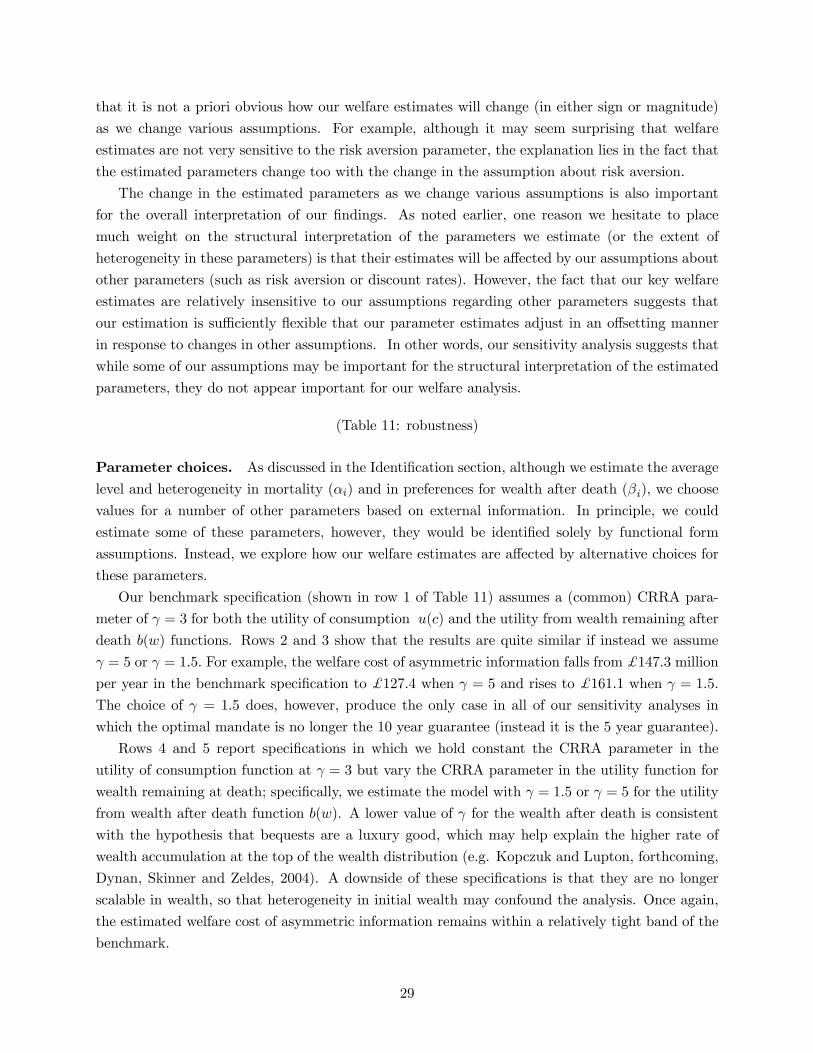
that it is not a priori obvious how our welfare estimates will change (in either sign or magnitude)

as we change various assumptions. For example, although it may seem surprising that welfare

estimates are not very sensitive to the risk aversion parameter, the explanation lies in the fact that

the estimated parameters change too with the change in the assumption about risk aversion.

The change in the estimated parameters as we change various assumptions is also important

for the overall interpretation of our findings. As noted earlier, one reason we hesitate to place

much weight on the structural interpretation of the parameters we estimate (or the extent of

heterogeneity in these parameters) is that their estimates will be affected by our assumptions about

other parameters (such as risk aversion or discount rates). However, the fact that our key welfare

estimates are relatively insensitive to our assumptions regarding other parameters suggests that

our estimation is sufficiently flexible that our parameter estimates adjust in an offsetting manner

in response to changes in other assumptions. In other words, our sensitivity analysis suggests that

while some of our assumptions may be important for the structural interpretation of the estimated

parameters, they do not appear important for our welfare analysis.

(Table 11: robustness)

Parameter choices. As discussed in the Identification section, although we estimate the average

level and heterogeneity in mortality (αi) and in preferences for wealth after death (βi), we choose

values for a number of other parameters based on external information. In principle, we could

estimate some of these parameters, however, they would be identified solely by functional form

assumptions. Instead, we explore how our welfare estimates are affected by alternative choices for

these parameters.

Our benchmark specification (shown in row 1 of Table 11) assumes a (common) CRRA para-

meter of γ = 3 for both the utility of consumption u(c) and the utility from wealth remaining after

death b(w) functions. Rows 2 and 3 show that the results are quite similar if instead we assume

γ = 5 or γ = 1.5. For example, the welfare cost of asymmetric information falls from £147.3 million

per year in the benchmark specification to £127.4 when γ = 5 and rises to £161.1 when γ = 1.5.

The choice of γ = 1.5 does, however, produce the only case in all of our sensitivity analyses in

which the optimal mandate is no longer the 10 year guarantee (instead it is the 5 year guarantee).

Rows 4 and 5 report specifications in which we hold constant the CRRA parameter in the

utility of consumption function at γ = 3 but vary the CRRA parameter in the utility function for

wealth remaining at death; specifically, we estimate the model with γ = 1.5 or γ = 5 for the utility

from wealth after death function b(w). A lower value of γ for the wealth after death is consistent

with the hypothesis that bequests are a luxury good, which may help explain the higher rate of

wealth accumulation at the top of the wealth distribution (e.g. Kopczuk and Lupton, forthcoming,

Dynan, Skinner and Zeldes, 2004). A downside of these specifications is that they are no longer

scalable in wealth, so that heterogeneity in initial wealth may confound the analysis. Once again,

the estimated welfare cost of asymmetric information remains within a relatively tight band of the

benchmark.

29

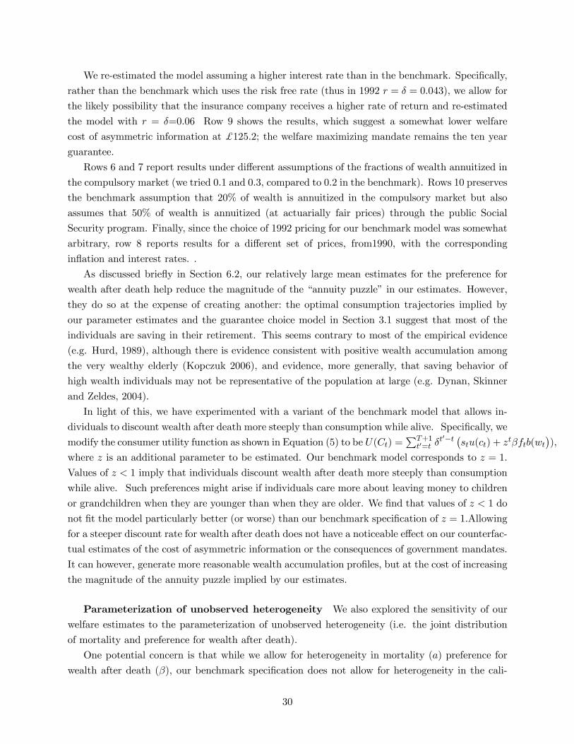
We re-estimated the model assuming a higher interest rate than in the benchmark. Specifically,

rather than the benchmark which uses the risk free rate (thus in 1992 r = δ = 0.043), we allow for

the likely possibility that the insurance company receives a higher rate of return and re-estimated

the model with r = δ=0.06 Row 9 shows the results, which suggest a somewhat lower welfare

cost of asymmetric information at £125.2; the welfare maximizing mandate remains the ten year

guarantee.

Rows 6 and 7 report results under different assumptions of the fractions of wealth annuitized in

the compulsory market (we tried 0.1 and 0.3, compared to 0.2 in the benchmark). Rows 10 preserves

the benchmark assumption that 20% of wealth is annuitized in the compulsory market but also

assumes that 50% of wealth is annuitized (at actuarially fair prices) through the public Social

Security program. Finally, since the choice of 1992 pricing for our benchmark model was somewhat

arbitrary, row 8 reports results for a different set of prices, from1990, with the corresponding

inflation and interest rates. .

As discussed briefly in Section 6.2, our relatively large mean estimates for the preference for

wealth after death help reduce the magnitude of the “annuity puzzle” in our estimates. However,

they do so at the expense of creating another: the optimal consumption trajectories implied by

our parameter estimates and the guarantee choice model in Section 3.1 suggest that most of the

individuals are saving in their retirement. This seems contrary to most of the empirical evidence

(e.g. Hurd, 1989), although there is evidence consistent with positive wealth accumulation among

the very wealthy elderly (Kopczuk 2006), and evidence, more generally, that saving behavior of

high wealth individuals may not be representative of the population at large (e.g. Dynan, Skinner

and Zeldes, 2004).

In light of this, we have experimented with a variant of the benchmark model that allows in-

dividuals to discount wealth after death more steeply than consumption while alive. Specifically, we

modify the consumer utility function as shown in Equation (5) to be U(Ct) =PT+1

t0=t δt0−t ¡stu(ct) + ztβftb(wt

¢),

where z is an additional parameter to be estimated. Our benchmark model corresponds to z = 1.

Values of z < 1 imply that individuals discount wealth after death more steeply than consumption

while alive. Such preferences might arise if individuals care more about leaving money to children

or grandchildren when they are younger than when they are older. We find that values of z < 1 do

not fit the model particularly better (or worse) than our benchmark specification of z = 1.Allowing

for a steeper discount rate for wealth after death does not have a noticeable effect on our counterfac-

tual estimates of the cost of asymmetric information or the consequences of government mandates.

It can however, generate more reasonable wealth accumulation profiles, but at the cost of increasing

the magnitude of the annuity puzzle implied by our estimates.

Parameterization of unobserved heterogeneity We also explored the sensitivity of our

welfare estimates to the parameterization of unobserved heterogeneity (i.e. the joint distribution

of mortality and preference for wealth after death).

One potential concern is that while we allow for heterogeneity in mortality (a) preference for

wealth after death (β), our benchmark specification does not allow for heterogeneity in the cali-

30

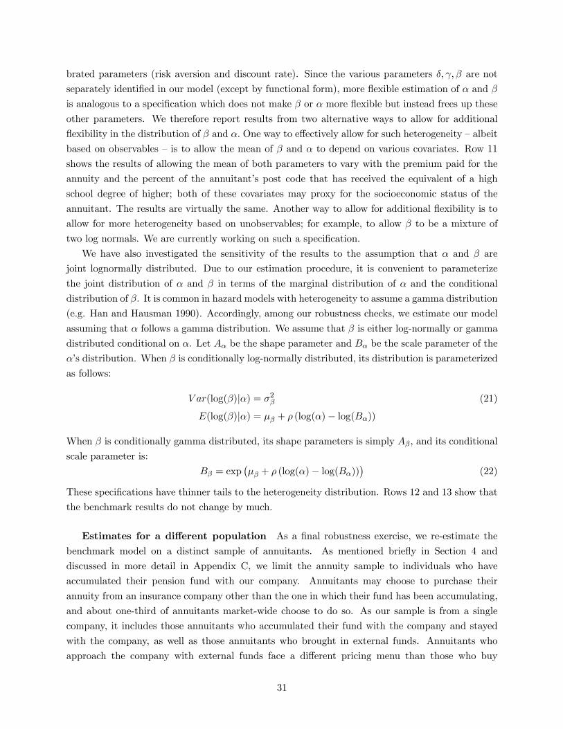
brated parameters (risk aversion and discount rate). Since the various parameters δ, γ, β are not

separately identified in our model (except by functional form), more flexible estimation of α and β

is analogous to a specification which does not make β or α more flexible but instead frees up these

other parameters. We therefore report results from two alternative ways to allow for additional

flexibility in the distribution of β and α. One way to effectively allow for such heterogeneity — albeit

based on observables — is to allow the mean of β and α to depend on various covariates. Row 11

shows the results of allowing the mean of both parameters to vary with the premium paid for the

annuity and the percent of the annuitant’s post code that has received the equivalent of a high

school degree of higher; both of these covariates may proxy for the socioeconomic status of the

annuitant. The results are virtually the same. Another way to allow for additional flexibility is to

allow for more heterogeneity based on unobservables; for example, to allow β to be a mixture of

two log normals. We are currently working on such a specification.

We have also investigated the sensitivity of the results to the assumption that α and β are

joint lognormally distributed. Due to our estimation procedure, it is convenient to parameterize

the joint distribution of α and β in terms of the marginal distribution of α and the conditional

distribution of β. It is common in hazard models with heterogeneity to assume a gamma distribution

(e.g. Han and Hausman 1990). Accordingly, among our robustness checks, we estimate our model

assuming that α follows a gamma distribution. We assume that β is either log-normally or gamma

distributed conditional on α. Let Aα be the shape parameter and Bα be the scale parameter of the

α’s distribution. When β is conditionally log-normally distributed, its distribution is parameterized

as follows:

V ar(log(β)|α) = σ2β (21)

E(log(β)|α) = μβ + ρ (log(α)− log(Bα))

When β is conditionally gamma distributed, its shape parameters is simply Aβ, and its conditional

scale parameter is:

Bβ = exp¡μβ + ρ (log(α)− log(Bα))

¢(22)

These specifications have thinner tails to the heterogeneity distribution. Rows 12 and 13 show that

the benchmark results do not change by much.

Estimates for a different population As a final robustness exercise, we re-estimate the

benchmark model on a distinct sample of annuitants. As mentioned briefly in Section 4 and

discussed in more detail in Appendix C, we limit the annuity sample to individuals who have

accumulated their pension fund with our company. Annuitants may choose to purchase their

annuity from an insurance company other than the one in which their fund has been accumulating,

and about one-third of annuitants market-wide choose to do so. As our sample is from a single

company, it includes those annuitants who accumulated their fund with the company and stayed

with the company, as well as those annuitants who brought in external funds. Annuitants who

approach the company with external funds face a different pricing menu than those who buy

31

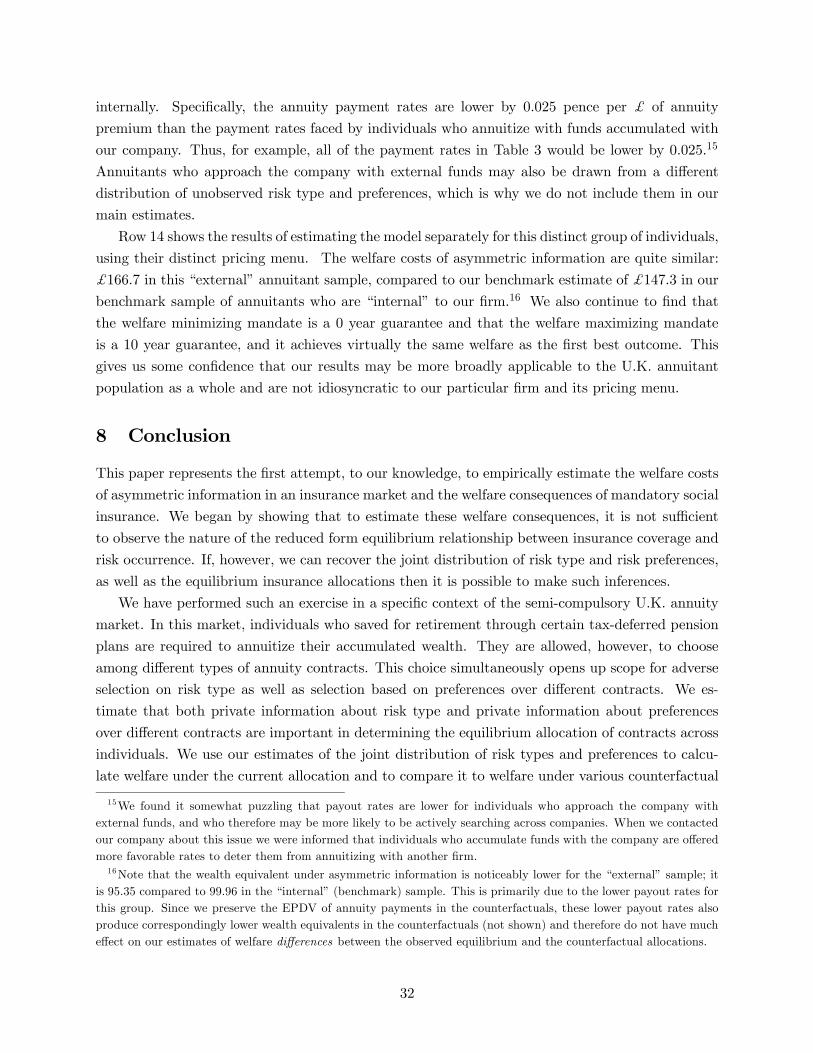
internally. Specifically, the annuity payment rates are lower by 0.025 pence per £ of annuity

premium than the payment rates faced by individuals who annuitize with funds accumulated with

our company. Thus, for example, all of the payment rates in Table 3 would be lower by 0.025.15

Annuitants who approach the company with external funds may also be drawn from a different

distribution of unobserved risk type and preferences, which is why we do not include them in our

main estimates.

Row 14 shows the results of estimating the model separately for this distinct group of individuals,

using their distinct pricing menu. The welfare costs of asymmetric information are quite similar:

£166.7 in this “external” annuitant sample, compared to our benchmark estimate of £147.3 in our

benchmark sample of annuitants who are “internal” to our firm.16 We also continue to find that

the welfare minimizing mandate is a 0 year guarantee and that the welfare maximizing mandate

is a 10 year guarantee, and it achieves virtually the same welfare as the first best outcome. This

gives us some confidence that our results may be more broadly applicable to the U.K. annuitant

population as a whole and are not idiosyncratic to our particular firm and its pricing menu.

8 Conclusion

This paper represents the first attempt, to our knowledge, to empirically estimate the welfare costs

of asymmetric information in an insurance market and the welfare consequences of mandatory social

insurance. We began by showing that to estimate these welfare consequences, it is not sufficient

to observe the nature of the reduced form equilibrium relationship between insurance coverage and

risk occurrence. If, however, we can recover the joint distribution of risk type and risk preferences,

as well as the equilibrium insurance allocations then it is possible to make such inferences.

We have performed such an exercise in a specific context of the semi-compulsory U.K. annuity

market. In this market, individuals who saved for retirement through certain tax-deferred pension

plans are required to annuitize their accumulated wealth. They are allowed, however, to choose

among different types of annuity contracts. This choice simultaneously opens up scope for adverse

selection on risk type as well as selection based on preferences over different contracts. We es-

timate that both private information about risk type and private information about preferences

over different contracts are important in determining the equilibrium allocation of contracts across

individuals. We use our estimates of the joint distribution of risk types and preferences to calcu-

late welfare under the current allocation and to compare it to welfare under various counterfactual

15We found it somewhat puzzling that payout rates are lower for individuals who approach the company withexternal funds, and who therefore may be more likely to be actively searching across companies. When we contactedour company about this issue we were informed that individuals who accumulate funds with the company are offeredmore favorable rates to deter them from annuitizing with another firm.16Note that the wealth equivalent under asymmetric information is noticeably lower for the “external” sample; it

is 95.35 compared to 99.96 in the “internal” (benchmark) sample. This is primarily due to the lower payout rates forthis group. Since we preserve the EPDV of annuity payments in the counterfactuals, these lower payout rates alsoproduce correspondingly lower wealth equivalents in the counterfactuals (not shown) and therefore do not have mucheffect on our estimates of welfare differences between the observed equilibrium and the counterfactual allocations.

32

allocations.

Our results suggest that, relative to a first-best symmetric information benchmark, the welfare

cost of asymmetric information along the dimension of guarantee choice is about 30 percent of the

maximum money at stake in this choice. These estimates account for about £145 million annually,

or about 2.5 percent of annual premia in the market. The estimates are quite stable across a range

of alternative assumptions.

We also find that government mandates that eliminate any choice among annuity contracts do

not necessarily improve on the asymmetric information equilibrium. We estimate that a mandated

annuity contract could increase welfare relative to the current equilibrium by as much as £145

million per year, or could reduce it by as much as £110 million per year, depending on what

contract is mandated. Moreover, the welfare maximizing choice for a mandated contract would

not be apparent to the government without knowledge of the joint distribution of risk type and

preferences. Our results therefore suggest that achieving welfare gains through mandatory social

insurance may be harder in practice than simple theory would suggest.

Although our analysis is specific to the U.K. annuity market, the approach we take could be

applied to estimating the efficiency costs of asymmetric information and the welfare consequences of

government intervention in other insurance markets. As seen, the data requirements for recovering

the joint distribution of risk type and preferences are data on the menu of choices each individual

faces, the contract each chooses, and a measure of each individual’s ex-post claims experience. Such

data are often available from individual surveys or from insurance companies. These data are now

commonly used to test for the presence of asymmetric information in insurance markets, including

automobile insurance (Chiappori and Salanie, 2000; Cohen and Einav, forthcoming), health insur-

ance (Cardon and Hendel, 2001), and long term care insurance (Finkelstein and McGarry, 2006),

as well as annuity markets.

Our analysis was made substantially easier by the assumption that moral hazard does not exist

in annuity markets. As discussed, this may be a reasonable assumption for the annuity market.

It may also be a reasonable assumption for several other insurance markets. For example, Cohen

and Einav (forthcoming) argue that moral hazard is unlikely to be present over small deductibles

in automobile insurance. Grabowski and Gruber (2005) present evidence that suggests that there

is no detectable moral hazard effect of long term care insurance on nursing home use. In such

markets, the approach in this paper can be straightforwardly adopted.

In other markets, such as health insurance, moral hazard is likely to play an important role.

Estimation of the efficiency costs of asymmetric information therefore requires some additional

source of variation in the data to identify the incentive effects of the insurance policies. One

natural source would be exogenous changes in the contract menu. Such variation may occur when

regulation requires changes in pricing, or when employers change the menu of health insurance plans

from which their employees can choose. Non-linear experience rating schemes may also introduce

useful variation in the incentive effects of insurance policies (Abbring, Chiappori and Pinquet

2003b). More generally, recent advances in using dynamic insurance data to separately identify

moral hazard effects (see e.g. Abbring et al., 2003a) likely provide a useful lever for extending our

33

approach to estimating welfare costs in insurance markets with moral hazard. In light of our current

work, we consider the application and extension of our approach to other markets, including those

with moral hazard, an interesting and important direction for further work.

9 References

Abbring, Jaap, James Heckman, Pierre-Andre Chiappori, and Jean Pinquet. 2003a. “Adverse

Selection and Moral Hazard in Insurance: Can Dynamic Data Help to Distinguish?”. Journal of

the European Economic Association Papers and Proceedings 1(2/3): 512-521.

Abbring, Jaap, Pierre-Andre Chiappori and Jean Pinquet. 2003b. “Moral hazard and Dynamic

Insurance Data.” Journal of the European Economic Association 1(4): 767-820.

Akerlof, George (1970), “The market for ’lemons’: quality uncertainty and the market mecha-

nism,” Quarterly Journal of Economics 84(3), 488-500.

Association of British Insurers. 1999. Insurance Statistics Year Book: 1986-1998.

Banks, James, and Carl Emmerson (1999), “U.K. Annuitants,” IFS Briefing Note, London:

Institute for Fiscal Studies.

Barsky, R. B., F. T. Juster, M. S. Kimball, and M. D. Shapiro (1997), “Preference parameters

and behavioral heterogeneity: An experimental approach in the Health and Retirement Study,”

Quarterly Journal of Economics 112(2), 537-579.

Braun, Michael, and Alexander Muermann (2004), “The Impact of Regret on The Demand for

Insurance,” Journal of Risk and Insurance 71(4), 737-767.

Brown, Jeffrey, and Amy Finkelstein (2006), ”The Interaction of Public and Private Insurance:

Medicaid and the Long-Term Care Insurance Market,” mimeo, MIT.

Brown, Jeffrey, Olivia Mitchell, James Poterba, and Mark Warshawsky (2001), The Role of

Annuity Markets in Financing Retirement, Cambridge, MA: MIT Press.

Cardon, James H., and Igal Hendel (2001), “Asymmetric Information in Health Insurance:

Evidence from the National Medical Expenditure Survey,” Rand Journal of Economics 32(3), 408-

427.

Chiappori, Pierre-Andre and Bernard Salanie (2000), “Testing for Asymmetric Information in

Insurance Markets,” Journal of Political Economy 108(1), 56-78.

Chiappori, Pierre-Andre, Bruno Jullien, Bernard Salanie, and Francois Salanie (forthcoming),

“Asymmetric Information in Insurance: General Testable Implications,” Rand Journal of Eco-

nomics, forthcoming.

Cohen, Alma, and Liran Einav (forthcoming), “Estimating risk preferences from deductible

choice,” American Economic Review, forthcoming.

Cox, David (1972), “Regression models and life-tables (with discussion),” Journal of the Royal

Statistical Society, Series B 34, 1987-220.

Cox, David (1975), “Partial Likelihood,” Biometrika 62, 269-276.

Cutler, David, and Richard Zeckhauser (2000), “The Anatomy of Health Insurance” in A. Culyer

and J. Newhouse, eds. Handbook of Health Economics, Volume IA, Amsterdam: Elsevier.

34

Davidoff, Thomas, and Gerd Welke (2005),.“Selection and moral hazard in the reverse mortgage

market,” mimeo, UC Berkeley.

Davidoff, Thomas, Jeffrey Brown, and Peter Diamond (2005) “Annuities and Individual Wel-

fare,” American Economic Review 95(5), 1573-1590.

Davis, S., Felix Kubler, and P. Willen (2006), “Borrowing Costs and the Demand for Equity

over the Life Cycle,” Review of Economics and Statistics 86(2), 348-362.

de Meza, David and Webb, David C. (2001), “Advantageous selection in insurance markets,”

Rand Journal of Economics 32(2), 249-262

Dynan, Karen, Jonathan Skinner and Stephen Zeldes. 2004. “Do the rich save more?”. Journal

of Political Economy April: 397-444.

Engen, Eric M., William G. Gale, and Cori R. Uccello (1999), “The Adequacy of Retirement

Saving,” Brookings Papers on Economic Activity 2, 65-165.

Fang, Hanming, Michael Keane, and Dan Silverman (2006), “Sources of Advantageous Selection:

Evidence from the Medigap Insurance Market,” mimeo, Yale University.

Feldstein, Martin (2005), “Rethinking Social Insurance,” NBER Working Paper No. 11250.

Finkelstein, Amy, and Kathleen McGarry (2006), “Multiple dimensions of private information:

evidence from the long-term care insurance market,” American Economic Review 96(4), 938-958.

Finkelstein, Amy, and James Poterba (2002), “Selection Effects in the Market for Individual

Annuities: New Evidence from the United Kingdom,” Economic Journal 112(476), 28-50.

Finkelstein, Amy, and James Poterba (2004), “Adverse Selection in Insurance Markets: Policy-

holder Evidence from the U.K. Annuity Market,” Journal of Political Economy 112(1), 193-208.

Finkelstein, Amy, and James Poterba (2006), “Testing for Adverse Selection with ’Unused

Observables’,” NBER Working Paper No. 12112.

Friedman, Benjamin M., and Mark J. Warshawsky (1990), “The Cost of Annuities: Implications

for Saving Behavior and Bequests,” Quarterly Journal of Economics 105(1), 135-154.

Grabowski, D. C., and J. Gruber (2005), “Moral Hazard in Nursing Home Use,” NBERWorking

Paper No. 11723.

Han, Aaron, and Jerry Hausman (1990), “Flexible Parametric Estimation of Duration and

Competing Risk Models,” Journal of Applied Econometrics 5, 1-28.

Heckman, J., and B. Singer (1984), “The Identifiability of the Proportional Hazard Model,”

Review of Economic Studies 51(2), 231-241.

Horiuchi, Shiro, and Ansley Coale (1982), “A simple Equation for Estimating the Expectation

of Life at Old Ages,” Population Studies 36, 317-326.

Hubbard, Glenn, Jonathan Skinner, and Stephen Zeldes (1995), “Precautionary Savings and

Social Insurance,” Journal of Political Economy 103(2), 360-99.

Hurd, Michael D. (1989), “Mortality Risk and Bequests,” Econometrica 57(4), 779-813.

Institute of Actuaries and Faculty of Actuaries, Continuous Mortality Investigation Committee.

1999. Continuous Mortality Investigation Reports, Number 17.

Jullien, Bruno, Bernard Salanie, and Francois Salanie (2002), “Screening risk-averse agents

under moral hazard,” mimeo, Columbia University.

35

Kopczuk, Wojciech and Joseph Lupton (forthcoming), “To Leave or not To Leave: The Distri-

bution of Bequest Motives,” Review of Economic Studies, forthcoming.

Kopczuk, Wojciech. 2006. “Bequest and tax planning: evidence from estate tax returns.”

Unpublished mimeo. Available at http://www.columbia.edu/~wk2110/bin/ill.pdf.

Kotlikoff, Lawrence J., and Avia Spivak (1981), “The Family as an Incomplete Annuities Mar-

ket,” Journal of Political Economy 89(2), 372-391.

Laibson, David I., Andrea Repetto, and Jeremy Tobacman (1998), “Self-control and saving for

retirement,” Brookings Papers on Economic Activity 1, 91-196.

Laitner, John, and Juster F. Thomas (1996), “New Evidence on Altruism: A Study of TIAA-

CREF Retirees,” American Economic Review 86(4), 893-908.

Meyer, Bruce (1990), “Unemployment Insurance and Unemployment Spells,” Econometrica

58(4), 757-782.

Mitchell, Olivia S., James M. Poterba, Mark Warshawsky, and Jeffrey R. Brown (1999), “New

Evidence on the Money’s Worth of Individual Annuities,” American Economic Review 89, 1299-

1318.

Miyazaki, H. (1977), “The Rat Race and Internal Labor Markets,” Bell Journal of Economics

8, 394-418.

Murthi, Mamta, J. Michael Orszag, and Peter Orszag (1999), “The Charge Ratio on Individual

Accounts: Lessons for the U.K. Experience,” Working Paper 99-2, Birkbeck College, University of

London.

Palumbo, Michael G. (1999), “Uncertain Medical Expenses and Precautionary Saving Near the

End of the Life Cycle,” Review of Economic Studies 66(2), 395—421.

Philipson, T., and G. Becker (1998) “Old-Age Longevity and Mortality Contingent Claims,”

Journal of Political Economy 106(3), 550-574.

Rothschild, Michael, and Joseph E. Stiglitz. 1976. “Equilibrium in Competitive Insurance

Markets: An Essay on the Economics of Imperfect Information,” Quarterly Journal of Economics

90, 630-649.

Scholz, John Karl, Ananth Seshadri, and Surachai Khitatrakun (2006), “Are Americans Saving

‘Optimally’ for Retirement?” Journal of Political Economy 114(4), 607-643.

Sheshinski, Eytan (2006), “Differentiated Annuities in a Pooling Equilibrium,” mimeo, Hebrew

University of Jerusalem.

Smart, Michael (2000), “Competitive insurance markets with two unobservables,” International

Economic Review 41(1), 153-169.

Spence, Michael (1978), “Product Differentiation and Performance in Insurance Markets,” Jour-

nal of Public Economics 10, 427-447.

Wambach, Achim (2000), “Introducing Heterogeneity in the Rothschild-Stiglitz Model,” Journal

of Risk and Insurance 67(4), 579-92.

36

Appendix

A Proofs

Proposition 1: π(pi,mi, ri) is increasing in pi, mi, and in ri.

Proof. π(pi,mi, ri) is given by

π(pi,mi, ri) =1

riln (1− pi + pie

rimi)

where ri > 0 and pi ∈ (0, 1). It is straight forward to verify that it is increasing in mi and in pi

(since rimi > 0 so erimi > 1). The more complicated part is to show that π(pi,mi, ri) is increasing

in ri. To see this, note that

∂π

∂ri=1

ri

∙pimie

rimi

1− pi + pierimi− 1

riln (1− pi + pie

rimi)

¸(23)

This implies that

sign

µ∂π

∂ri

¶= sign [ripimie

rimi − (1− pi + pierimi) ln (1− pi + pie

rimi)] (24)

To simplify, we drop i subscripts and denote θ ≡ erm − 1 > 0. Then we can rewrite equation

(24) as

sign

µ∂π

∂r

¶= sign [p(θ + 1) ln(θ + 1)− (1 + pθ) ln (1 + pθ)] (25)

Let f(p, θ) ≡ p(θ + 1) ln(θ + 1) − (1 + pθ) ln (1 + pθ). We will show that f(p, θ) > 0 for any

θ > 0 and p ∈ (0, 1). First, note that f(0, θ) = 0 and f(1, θ) = 0. Second, note that ∂f∂p =

(θ + 1) ln(θ + 1)− θ − θ ln (1 + pθ) which is positive at p = 0 (for any θ > 0)17. Finally, note that∂2f∂p2 = −

θ2

1+pθ < 0 so f(p, θ) is concave in p and therefore can cross the horizontal axis only once

more. Thus, since f(p, θ) = 0 for p = 1, it has to be that f(p, θ) lies above the horizontal axis for

all p ∈ (0, 1).See appendix.Proposition 2: π(pi,mi, ri) −mipi is positive, is increasing in mi and in ri, and is initially

increasing and then decreasing in pi.

Proof. π(pi,mi, ri)− pimi is given by

f(pi,mi, ri) =1

riln (1− pi + pie

rimi)− pimi

where ri > 0 and pi ∈ (0, 1). From proposition 1, we know tat it is increasing in ri.

To see that it is increasing in mi, note that

∂f

∂mi=1

ri

pirierimi

1− pi + pierimi− pi =

pi(erimi − 1)(1− pi)

1− pi + pierimi> 0 (26)

17To see this, let g(θ) ≡ (θ + 1) ln(θ + 1)− θ. g(0) = 0 and g0(θ) = 1 + ln(θ + 1)− 1 = ln(θ + 1) which is positivefor any θ > 0.

37

Finally, to see that it is initially increasing and then decreasing in pi, note that

∂f

∂pi=1

ri

erimi − 11− pi + pierimi

−mi =(erimi − 1)(1−miripi)− rimi

ri (1− pi + pierimi)(27)

Let θ ≡ rimi > 0, and note that sign³∂f∂pi

´= sign(g(θ, pi)) where g(θ, p) = (eθ−1)(1−θp)−θ.

Then note that g(θ, 0) = eθ − 1− θ > 0 for all θ > 0 since g(0, 0) = 0 and ∂g(θ,0)∂θ = eθ − 1 > 0, and

that g(θ, 1) = (eθ − 1)(1− θ) − θ < 0 since g(0, 1) = 0 and ∂g(θ,1)∂θ = −eθθ < 0. Finally, note that

∂g∂p = −θ(eθ − 1) is always negative.Proposition 4 In any pure strategy Nash equilibrium, profits are zero.Proof. Let πj be the equilibrium price set by firm j. If firm j makes negative profits, it has

a profitable deviation to πj > πk where it does not sell and makes zero profits. If firm j makes

positive profits then it has to be the case that πk ≥ πj (otherwise firm j’s profits are zero). In such

a case, firm k has a profitable deviation to πj − for > 0 sufficiently small. This will make firm

k earn higher profits.

Proposition 5 If mp∗ + F < min(πL, πH) the unique equilibrium is the pooling equilibrium,

πPool = mp∗ + F .

Proof. We only need to consider other zero-profit prices. Any such price must sell to eithertype L or type H but not to both. However, since πPool < min(πL, πH) then setting πPool + for

> 0 sufficiently small will attract all consumers and make positive profits, which would constitute

a profitable deviation.

Proposition 6 If mp∗ + F > min(πL, πH) the unique equilibrium with positive demand, if it

exists, is to set π = mpθ + F and serve only type θ, where θ = H (L) if πL < πH (πH < πL).

Proof. The pooling price cannot attract both types, and therefore it (generically) cannot makezero profits and constitute an equilibrium. without loss of generality, suppose that πL < πH . In

such a case, any price that attracts type L will also attract type H. Therefore, the only possible

equilibrium is to sell insurance to type H for the zero profits price, mpH + F . If mpH + F > πH

then there is no equilibrium with positive demand.

Proposition For each case described in Table 1, the set of parameters that satisfy the para-

meter restrictions is not empty.

Proof. The proof relies on Table A1 below, which provides the parameter restrictions for allcases.

Consider case 1. For simplicity, suppose F = 0 and no preference heterogeneity (rH = rL).

Since the risk premium is always positive, all we need is that πL < p∗m. Since p∗ is an increasing

function of pH and λH but πL is not, it is easy to see that with pL sufficiently low and pH and λH

sufficiently high, the inequality will be satisfied.

Consider case 2. Suppose that F > 0 is small enough that πH ≥ F + pHm is still satisfied (e.g.

because rH , and therefore the risk premium for H, is high). It is easy to see that for any F > 0

there exists rL sufficiently small below which the risk premium for L is lower than F .

Consider case 3. Suppose rH is small, so the risk premium for H is lower than F , and suppose

that rL is high enough so the risk premium for L is greater than F . It is easy to see that if pH is

38

sufficiently greater than pL (e.g. think of pH close to 1 and of pL close to 0), there is an intermediate

value for rH that will make H still buy insurance at the pooling price (despite F ) and rL sufficiently

high that will still make L buy.

Consider case 4. Suppose that rH is sufficiently low and F > 0 is high enough, that H will not

buy insurance even for a price of pL.

Table A1: Parameter conditions for each case

Efficient Outcome Equilibrium Outcome Binding ConstraintsNecessary

Conditions

1

(πL ≥ F + pLm

πH ≥ F + pHm

(πL < F + p∗m

πH ≥ F + pHm

πL − pLm ∈ [F,F + λH(pH − pL)m)

πH − pHm ≥ F−

2

(πL < F + pLm

πH ≥ F + pHm

(πL < F + p∗m

πH ≥ F + pHm

πL − pLm < F

πH − pHm ≥ FF > 0

3

(πL ≥ F + pLm

πH < F + pHm

(πL ≥ F + p∗m

πH ≥ F + p∗m

πL − pLm ≥ F + λH(pH − pL)m

πH − pHm ∈ [F − λL(pH − pL)m,F )F > 0

4

(πL ≥ F + pLm

πH < F + pHm

(πL ≥ F + pLm

πH < F + pLm

πL − pLm ≥ F

πH − pHm < F − (pH − pL)m

F > 0

rL > rH

Proposition 7The solution to the utility function is homogeneous in w, i.e. for g∗(w0) =

g∗(λw0).

XX To be completed. What follows is just a sketch XX

Let V G1 (w) be the value function as of period 1 given initial wealth w and guarantee choice of

G.

Definition: Let the wealth equivalent (weq) be the addition to initial wealth for a person with

no guarantee that would make him indifferent between no guarantee and a five year guarantee.

Formally: weq = {V G=01 (w + x) = V G=5

1 (w)}. Note:(1) V () is monotone in w so x is uniquely

defined. (2) x may be either positive or negative depending on the parameters of the problem, and

in particular on the guarantee pricing (how fast Z declines with G).

Definition: The problem is scalable iff x/w is independent of w.

The “big” optimization problem (after change of variables):

maxwt’s

T+1Xt=0

δtµstU(wt + Zt −

wt+1

1 + r) + βtftB(wt + gt)

¶subject to a budget constraint and non-negativity constraints for the wt’s.

If annuity payments are linear function of w0 then we can now rewrite Zt = ktw0 and gt = ltw0.

One could now apply a change of variables — w∗t =wtw0— to make the optimization problem

identical to solving

maxw∗t ’s

T+1Xt=0

δtµstU(w

∗t + kt −

w∗t+11 + r

) + βtftB(w∗t + lt)

¶

39

since the w0 drops out from the budget constraint and can be taken out of the max (just multiplies

everything, as long as B and U use the same γ).

Thus, w∗t =wtw0is independent of w0, so the problem as a whole can be normalized by w0.

B Computation details

B.1 Likelihood

This section describes the details of the likelihood calculation. Recall from Section 3.2 that the log

likelihood is:

L(μ,Σ, λ) =NXi=1

log

Zlmi (α)l

gi (α)

1

σαφ

µlogα− μα

σα

¶dα (28)

where lmi (α) is the likelihood of individual i’s mortality experience conditional on α and lgi (α) is

the likelihood of individual i’s guarantee choice conditional on α. For completeness, we repeat the

formulas for lmi and lgi :

lmi (α) =³αeλti exp

³αλ(eλci − eλti)

´´di ³exp

³αλ(eλci − eλti)

´´1−di(29)

lgi (α) =Φ

Ãlog(βgi,gi+5(α, λ))− μβ|α

σβ|α

!− Φ

Ãlog(βgi−5,gi(α, λ))− μβ|α

σβ|α

!(30)

where μβ|α = μβ +σα,βσ2α(logα− μα) and σβ|α =

rσ2β −

σ2α,βσ2α.

We calculate the integral in equation 28 by quadrature. Let {xj}Mj=1 and {wj}Mj=1 beM quadra-

ture points and weights for integrating from −∞ to ∞. Person i’s contribution to the likelihood

is:

Li(μ,Σ, λ) =MXj=1

lmi (exjσα+μα)lgi (e

xjσα+μα)φ(xj)wj (31)

We maximize the likelihood using a gradient based searched. Although we could simply use

finite difference approximations for the gradient, greater accuracy and efficiency can be obtained

by programming the analytic gradient.

The derivative of the log likelihood with respect to one of the parameters, θ, is given by:

∂L∂θ

=NXi=1

1

Li(μ,Σ, λ)

⎡⎣ MXj=1

⎛⎝ ³∂lmi (α(xj))

∂α lgi (α(xj)) + lmi (α(xj))∂lgi (α(xj))

∂α

´∂α(xj)∂θ +

+∂lmi (α(xj))

∂θ lgi (α(xj)) + lmi (α(xj))∂lgi (α(xj))

∂θ

⎞⎠φ(xj)wj

⎤⎦

40

where α(xj) = exjσα+μα . The derivatives of lmi are:

∂lmi∂α

=

⎧⎨⎩lmi (α)¡1 + α

λ (eλci − eλti)

¢if di = 1

lmi (α)αλ (e

λci − eλti) if di = 0

∂lmi∂λ

=

⎧⎨⎩lmi (α)³ti +

αλ (cie

λci − tieλti)− α

λ2(cie

λci − tieλti)´

if di = 1

lmi (α)³αλ (cie

λci − tieλti)− α

λ2(cie

λci − tieλti)´

if di = 0

∂lmi∂θ

=0 for all other parameters

The derivatives of lgi are:

∂lgi∂α

=φ

Ãlog(βgi,gi+5(α, λ))− μβ|α

σβ|α

!Ã∂ log(βgi,gi+5)

∂α− σα,β

σ2αα

!

− φ

Ãlog(βgi−5,gi(α, λ))− μβ|α

σβ|α

!Ã∂ log(βgi−5,gi)

∂α− σα,β

σ2αα

!∂lgi∂μα

=φ

Ãlog(βgi,gi+5(α, λ))− μβ|α

σβ|α

!σα,βσ2α− φ

Ãlog(βgi−5,gi(α, λ))− μβ|α

σβ|α

!σα,βσ2α

∂lgi∂σα

=φ

Ãlog(βgi,gi+5(α, λ))− μβ|α

σβ|α

!Ãσα,βσ3αα

−log(βgi,gi+5(α, λ))− μβ|α

σ2β|α

σ2α,βσ3α

!

− φ

Ãlog(βgi−5,gi(α, λ))− μβ|α

σβ|α

!Ãσα,βσ3αα

−log(βgi−5,gi(α, λ))− μβ|α

σ2β|α

σ2α,βσ3α

!∂lgi∂μβ

=φ

Ãlog(βgi,gi+5(α, λ))− μβ|α

σβ|α

!− φ

Ãlog(βgi−5,gi(α, λ))− μβ|α

σβ|α

!∂lgi∂σβ

=φ

Ãlog(βgi,gi+5(α, λ))− μβ|α

σβ|α

!log(βgi,gi+5(α, λ))− μβ|α

σ2β|ασβ

− φ

Ãlog(βgi−5,gi(α, λ))− μβ|α

σβ|α

!log(βgi−5,gi(α, λ))− μβ|α

σ2β|ασβ

∂lgi∂σα,β

=φ

Ãlog(βgi,gi+5(α, λ))− μβ|α

σβ|α

!Ãlog(βgi,gi+5(α, λ))− μβ|α

σ2β|α

σα,βσ2α− logα

σ2α

!

− φ

Ãlog(βgi−5,gi(α, λ))− μβ|α

σβ|α

!Ãlog(βgi−5,gi(α, λ))− μβ|α

σ2β|α

σα,βσ2α− logα

σ2α

!

The derivatives of α(xj) are:

∂α(xj)

∂μα=α(xj)

∂α(xj)

∂σα=α(xj)xj

∂α(xj)

∂θ=0 for all other parameters

41

B.2 Guarantee Indifference Curves

As mentioned in the main text of the paper, the most difficult part of calculating the likelihood is

finding the points where people are indifferent between a g and g + 5 year guarantee, βg,g+5(α, λ).

To find these points we need to compute the expected utility associated with each guarantee length.

B.2.1 Value Function

The value of a guarantee of length g with payments zgt is:

V (g, α, β) =maxct,wt

TXt=0

st(α)δt c1−γt

1− γ+ βft(α)δ

t (wt +Ggt )1−γ

1− γ

s.t. 0 ≤ wt+1 = (wt + zgt − ct)(1 + r) (32)

where δ is the discount factor, r is the interest rate, and Ggt =

⎧⎨⎩Pg

s=tzgt

(1+r)s−t if t ≤ g

0 if t > gis the

present discount value of guaranteed future payments at time t. Also, st(α) is the probability of

being alive at time t and ft(α) is the probability of dying at time t. Note that a person who

dies at time t, dies before consuming ct or receiving zgt . Technically, there are also non-negativity

constraints on wealth and consumption. However, these constraints will never bind due to the form

of the utility function.

One could view (32) as a finite horizon discrete time dynamic programming problem and solve

it by discretize the state space (wt) and using backward induction. This was the approach that

we initially took. However, it was very time consuming to compute the value function to an

acceptable level of accuracy using this method. Consequently, we instead approached (32) as

a static optimization problem and used the first order conditions to collapse the problem to a

numerical optimization over a single variable, consumption at time zero. The first order conditions

for (32) are:

δtst(α)c−γt =λt ∀t ∈ {0..T} (33)

δtft(α)β(wt +Ggt )−γ =− λt +

1

1 + rλt−1 ∀t ∈ {1..T} (34)

(wt + zt − ct)(1 + r) =wt+1 ∀t ∈ {0..T − 1} (35)

where λt is the multiplier on the budget constraint at time t. Initial wealth, w0 is taken as given.

It is not possible to completely solve the first order conditions analytically. However, suppose we

knew c0. Then from the budget constraint (35), we can calculate w1. From the first order condition

for c0 (33), we can find λ0.

λ0 = s0(α)δ0c−γ0

We can use the first order condition for w1 to solve for λ1.

λ1 = −m1(α)δ1β(w1 +Gg

1)−γ +

1

1 + rλ0

42

Then, λ1 and the first order condition for ct gives c1.

c1 =

µλ1

δ1s1(α)

¶−1/γContinuing in this way, we can find the whole path of optimal ct and wt associated with the chosen

c0. If this path satisfies the non-negativity constraints on consumption and wealth, then we have

defined a value function of c0, V (c0, g, α, β). Thus, we can reformulate the optimal consumption

problem as an optimization problem over one variable.

maxc0

V (c0, g, α, β) (36)

Numerically maximizing a function of a single variable is a relatively easy problem and can be done

quickly and robustly. We solve (36) using a simple bracket and bisection method. To check our

program, we compared the value function as computed in this way and by our initial discretization

and backward induction approach. They agreed up to the expected precision.

B.2.2 Computing the Guarantee Indifference Curves

The guarantee indifference curves, βg,g+5(α, λ), are defined as the solution to:

V (g, α, βg,g+5(α, λ)) = V (g + 5, α, βg,g+5(α, λ))

For each α, we solve for βg,g+5(α, λ)) using a simple bisective search. Each evaluation of the

likelihood requires βg,g+5(α(xj), λ)) at each integration point xj . Maximizing the likelihood requires

searching over μα and σα, which will shift α(xj). As mentioned in the main text, rather than

recomputing βg,g+5(α(xj), λ)) each time α(xj) changes, we initially compute βg,g+5(α, λ)) on a

dense grid of α values and log-linearly interpolate as needed.

C Data Details

C.1 Annuitant sample

As mentioned in the text, we restrict our sample in several ways:

• As is common in the analysis of annuitant choices, we limit the sample to the approximatelysixty percent of annuities that insure a single life. The mortality experience of the single

life annuitant provides a convenient ex-post measure of risk type; measuring the risk type of

a joint life policy which insures multiple lives is less straightforward (Mitchell et al., 1999,

Finkelstein and Poterba 2004, 2006).

• We also restrict the sample to the approximately eighty percent of annuitants who hold onlyone annuity policy, since characterizing the features of the total annuity stream for individuals

who hold multiple policies is more complicated. Finkelstein and Poterba (2006) make a similar

restriction.

43

• We focus on the choice of guarantee period and abstract from a number of other dimensions

of individuals’ choices.

— Individuals can choose the timing of their annuitization, although they cannot annuitizebefore age 50 (45 for women) or delay annuitizing past age 75 (70 for women). We

estimate the model separately for different purchase ages, but do not explicitly model

the timing choice.

— Annuitants may also take a tax-free lump sum of up to 25 percent of the value of the

accumulated assets. We do not observe this decision — we observe only the amount

annuitized — and therefore do not model it. However, because of the tax advantage of

the lump sum — income from the annuity is treated as taxable income — it is likely that

most individuals fully exercise this option, and ignoring it is therefore unlikely to be a

concern.

— To simplify the analysis, we analyze policies with the same payment profile, restrictingour attention to the 90 percent of policies that pay a constant nominal payout (rather

than payouts that escalate in nominal terms). As an ancillary benefit, this may make

our assumption that individuals all have the same discount rate more realistic.

— We also drop the less than 1 percent of guaranteed policies which choose a guaranteelength other than 5 or 10 years.

• We limit our sample of annuitants to those who purchased a policy between January 1 1988and December 31 1994. Although we also have data on annuitants who purchased a policy

in 1995 - 1998, the firm altered its pricing policy in 1995. An exogenous change in the

pricing menu might provide a useful source of variation in estimating the model. However,

if the pricing change arose due to changes in selection of individuals into the firm — or if it

affects subsequent selection into the firm — using this variation without allowing for changes

in the underlying distribution of the annuitant parameters (i.e. in the joint distribution of

β and α) could produce misleading estimates. We therefore limit the sample to the about

one-half of annuities purchased in the pre-1995 pricing regime. In principle, we could also

separately estimate the model for the annuities purchased in the post-1995 pricing regime. In

practice, the small number of deaths among these more recent purchasers created problems

for estimation in this sample.

• We limit our sample to annuitants who purchsed an annuity with a pension fund that theyhad accumulated within our company. Annuitants may choose to purchase their annuity from

an insurance company other than the one in which their fund has been accumulating, and

about one-third of annuitants market-wide choose to do so. As our sample is from a single

company, it includes those annuitants who accumulated their fund with the company and

stayed with the company, as well as those annuitants who brought in external funds. We

limit our main analysis to the approximately two-thirds of individuals in our sample who

44

accumulated their funds with the company. In the Robustness Section, we re-estimate the

model for the one-third of individuals who brought in external funds, and find similar welfare

estimates.

• Because the pricing of different guarantees varies with the annuitant’s gender and age atpurchase, we conduct the analysis separately for different age-gender combinations. We limit

our sample of annnuitants to those who purchased at the two most common ages of 60 or 65.

About three-fifths of our sample purchased their annuity at 60 or 65. Sample sizes for other

age-gender cells are too small for estimation purposes.

C.2 Time varying annuity pricing

As discussed in Section 4, the menu of annuity payment rates per pound of annuity premium

varies over time due to changes in interest rates. Using the temporal variation in annuity rates to

estimate the model creates a practical problem as the term structure the company faces is likely to

be correlated with time varying components of the value functions individuals use when making their

guarantee choices. Use of the time-varying annuity rates therefore requires us to make assumptions

about the time-varying components of the value function. In particular, we must make assumptions

about the interest rates that individuals use in making their guarantee choices, and whether the

discount rate δ by which individuals discount future consumption is a time-invariant individual

characteristic or moves in lock step with interest rates (so that changes in interest rates did not

affect the individual’s optimal consumption path). The failure of either of these assumptions could

substantially confound our analysis. Indeed, when we experimented with a version of the model

in which we assumed that individuals use the nominal risk free interest rate and that individual

discount rates moved in lock set with this interest rate, we found that the indifference sets for the

optimal guarantee choice moved a lot more than actual choices, which creates practical estimation

problems and suggests our assumptions were unlikely to be correct.

Given these issues, our imperfect solution is to analyze the choice problem with respect to

one particular pricing menu. This, of course, still requires assumptions about the interest rate to

use and addresses the issue of the time-varying nature of the individuals’ value functions only by

assuming it away. In principle, there is no a priori reason to prefer this approach. However, in

practice, it produces substantially more stable and reasonable estimates.

45

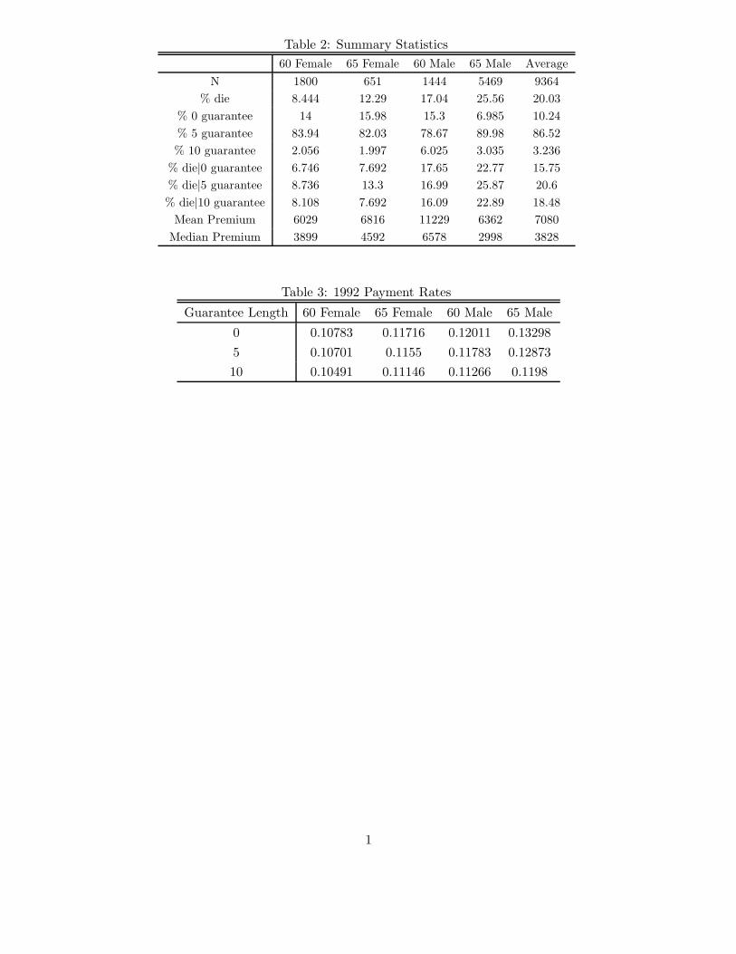
Table 2: Summary Statistics

60 Female 65 Female 60 Male 65 Male Average

N 1800 651 1444 5469 9364

% die 8.444 12.29 17.04 25.56 20.03

% 0 guarantee 14 15.98 15.3 6.985 10.24

% 5 guarantee 83.94 82.03 78.67 89.98 86.52

% 10 guarantee 2.056 1.997 6.025 3.035 3.236

% die|0 guarantee 6.746 7.692 17.65 22.77 15.75

% die|5 guarantee 8.736 13.3 16.99 25.87 20.6

% die|10 guarantee 8.108 7.692 16.09 22.89 18.48

Mean Premium 6029 6816 11229 6362 7080

Median Premium 3899 4592 6578 2998 3828

Table 3: 1992 Payment Rates

Guarantee Length 60 Female 65 Female 60 Male 65 Male

0 0.10783 0.11716 0.12011 0.13298

5 0.10701 0.1155 0.11783 0.12873

10 0.10491 0.11146 0.11266 0.1198

1

Table 4: Parameter Estimates

60 Female 65 Female 60 Male 65 Male

N 1800 651 1444 5469

µα -5.797 -5.679 -4.972 -5.267

(0.002731) (0.004832) (0.001799) (0.0003923)

σα 0.1412 0.19 0.06619 0.04142

(0.05599) (0.04131) (0.09606) (0.06881)

λ 0.1241 0.09991 0.1179 0.1283

(4.111e-06) (1.197e-05) (2.493e-06) (1.208e-07)

µβ 9.752 9.528 9.695 10.24

(0.004287) (0.1387) (0.004144) (0.0009836)

σβ 0.144 0.1891 0.2993 0.218

(0.1526) (3.854) (0.02572) (0.01521)

ρ -0.7807 -0.9979 -0.8964 -0.1704

(0.04603) (1.014) (0.02267) (0.1005)

Note: γ = 3,r = 0.043, δ = 0.043, π = 0.05

This table shows parameter estimates for each of the four groups. Standard errors are in parentheses.

2

Table 5: Fit of the Model60 Female 65 Female

Guarantee Length

All 0 5 10

Proportion

Observed — 0.14 0.8394 0.02056

Estimated — 0.14 0.8394 0.0206

Probability of Death

Observed 0.08444 0.06746 0.08736 0.08108

Estimated 0.08483 0.07111 0.08646 0.1115

Expected Payment

19.66 19.97 19.63 19.04

Interest rate such that company breaks even = 0.04064

Guarantee Length

All 0 5 10

Proportion

— 0.1598 0.8203 0.01997

— 0.1596 0.8202 0.02013

Probability of Death

0.1229 0.07692 0.133 0.07692

0.1236 0.09319 0.128 0.1851

Expected Payment

20.18 20.69 20.1 19.21

Interest rate such that company breaks even = 0.04378

60 Male 65 Male

Guarantee Length

All 0 5 10

Proportion

Observed — 0.153 0.7867 0.06025

Estimated — 0.1531 0.7867 0.06027

Probability of Death

Observed 0.1704 0.1765 0.1699 0.1609

Estimated 0.1721 0.1832 0.1708 0.1601

Expected Payment

20.13 20.17 20.14 19.79

Interest rate such that company breaks even = 0.04346

Guarantee Length

All 0 5 10

Proportion

— 0.06985 0.8998 0.03035

— 0.06984 0.8998 0.03036

Probability of Death

0.2556 0.2277 0.2587 0.2289

0.258 0.2536 0.2581 0.2652

Expected Payment

20.63 21.16 20.62 19.72

Interest rate such that company breaks even = 0.04714

This table summarizes the fit of our estimates. The first two rows of each cell report the observed and estimated

proportion of people who choose each guarantee length. The next three rows report observed and estimated prob-

abilities of death. The estimated probabilities of death take into the fact that our data is censored and truncated.

The estimated overall probability of death is computed as the average of:

Z

1 −S(α, λ, a2005

i )

S(α, λ, a1998i )

f(α)dα (1)

where a1998i and a2005

i are the ages of person i at the start and end of our sample period. The second of these three

rows reports the estimated probabilities of death conditional on predicted guarantee:

1

P (gi = g)

Z

1 −S(α, λ, a2005

i )

S(α, λ, a1998i )

!

P (gi = g|α)f(α)dα (2)

The last of these three rows reports the estimated probability of death conditional on observed guarantee choice. In

other words, the average of (2) among people who actually chose each guarantee.

The expected present discounted value of payments conditional on α and β is computed as:

E(pay) =

g∗(α,β)X

t=1

zg∗(α,β)t

(1 + r)t+

TX

t=1

zt

(1 + r)tS(α, λ, t) (3)

where g∗(α, β) is the optimal guarantee length given α and β. In the four columns, we report the average expected

payment both overall and conditional on each guarantee length.

The final row of each cell reports the interest rate such that the average overall expected payment is equal to 20,

the amount of the premium.

3

Table 6: Life Expectancies

Percentile 60 Female 65 Female 60 Male 65 Male

5 87.86 92.21 81.67 82.24

50 86.13 89.39 80.87 81.77

95 84.42 86.61 80.08 81.3

From Mortality Table 82.47 83.26 78.87 79.98

In this table, we use the estimates in table 4 to compute life expectancies. The first five rows of this table

report life expectancies conditional on a given value of α. They are meant to illustrate the degree of heterogeneity in

mortality. The second last row integrates over the distribution of α to compute an average estimated life expectancy.

The final row reports the UK pensioner average life expectancy for comparison. This average is based on the male

and female 1992 period tables for “life office pensioners” (Institute of Actuaries, 1999).

Table 7: Wealth Equivalents of the Observed Equilibrium

60 Female 65 Female 60 Male 65 Male Average

Current (asymm. info) 99.948 100.99 100.08 99.786 99.96

% Vol. Annuitize 0.415 0.998 0.6824 0.1844 0.3621

The first row of this table shows estimated average wealth equivalents of the annuities under the observed

asymmetric information equilibrium. The column labeled average is an average weighted by sample size. We define

the wealth equivalent of an annuity as the amount of wealth per 100 £ of initial wealth that we would have to give a

person without an annuity for them to be as well off as with 20% of their initial wealth annuitized. The second row

of the table shows the percentage of people who would voluntarily annuitize, i.e. the percentage of wealth equivalents

that are greater than 100 £.

4

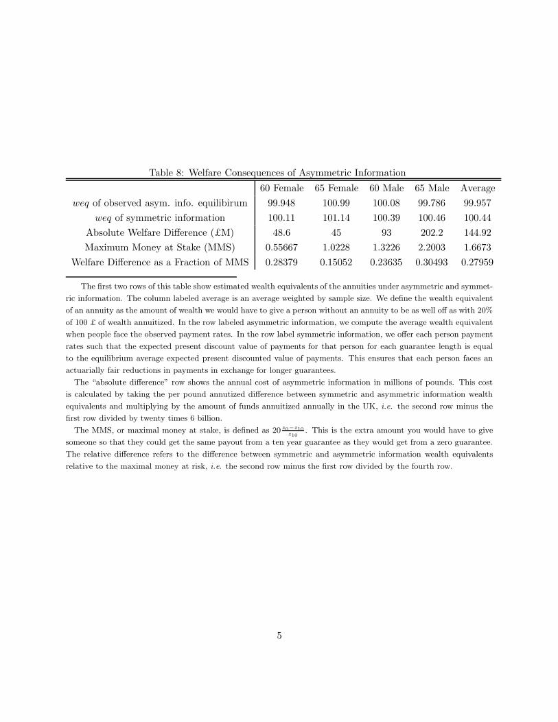
Table 8: Welfare Consequences of Asymmetric Information

60 Female 65 Female 60 Male 65 Male Average

weq of observed asym. info. equilibirum 99.948 100.99 100.08 99.786 99.957

weq of symmetric information 100.11 101.14 100.39 100.46 100.44

Absolute Welfare Difference (£M) 48.6 45 93 202.2 144.92

Maximum Money at Stake (MMS) 0.55667 1.0228 1.3226 2.2003 1.6673

Welfare Difference as a Fraction of MMS 0.28379 0.15052 0.23635 0.30493 0.27959

The first two rows of this table show estimated wealth equivalents of the annuities under asymmetric and symmet-

ric information. The column labeled average is an average weighted by sample size. We define the wealth equivalent

of an annuity as the amount of wealth we would have to give a person without an annuity to be as well off as with 20%

of 100 £ of wealth annuitized. In the row labeled asymmetric information, we compute the average wealth equivalent

when people face the observed payment rates. In the row label symmetric information, we offer each person payment

rates such that the expected present discount value of payments for that person for each guarantee length is equal

to the equilibrium average expected present discounted value of payments. This ensures that each person faces an

actuarially fair reductions in payments in exchange for longer guarantees.

The “absolute difference” row shows the annual cost of asymmetric information in millions of pounds. This cost

is calculated by taking the per pound annutized difference between symmetric and asymmetric information wealth

equivalents and multiplying by the amount of funds annuitized annually in the UK, i.e. the second row minus the

first row divided by twenty times 6 billion.

The MMS, or maximal money at stake, is defined as 20 z0−z10

z10. This is the extra amount you would have to give

someone so that they could get the same payout from a ten year guarantee as they would get from a zero guarantee.

The relative difference refers to the difference between symmetric and asymmetric information wealth equivalents

relative to the maximal money at risk, i.e. the second row minus the first row divided by the fourth row.

5

Table 9: Welfare Consequences of Government Mandates

60 Female 65 Female 60 Male 65 Male Average

weq of observed asym. info. equilibirum 99.948 100.99 100.08 99.786 99.957

weq of Mandated 0 99.849 100.86 99.832 99.262 99.584

Absolute Welfare Diff. (£M) -29.7 -39 -74.4 -157.2 -111.72

Welfare Diff. as a Fraction of MMS -0.17761 -0.12717 -0.18912 -0.23812 -0.21124

weq of Mandated 5 99.958 101.01 100.08 99.788 99.961

Absolute Welfare Diff. (£M) 3 6 0 0.6 1.3444

Welfare Diff. as a Fraction of MMS 0.018331 0.022213 0.0015903 0.00095563 0.005872

weq of Mandated 10 100.11 101.14 100.39 100.46 100.44

Absolute Welfare Diff. (£M) 48.6 45 93 202.2 144.92

Welfare Diff. as a Fraction of MMS 0.2836 0.15067 0.23538 0.30488 0.27938

Here, we report the average wealth equivalent when everyone is forced to purchase the same guarantee length.

We define the wealth equivalent of an annuity as the amount of wealth we would have to give a person without

an annuity to be as well off as with 20% of 100 £ of wealth annuitized. Under each mandate, we set the payment

rate such that the overall average expected payment is equal to the average expected payment under asymmetric

information and optimal guarantee choices. The column labeled average is an average weighted by sample size.

The “absolute difference” rows show the annual benefit of switching to the given counterfactual. This cost is

calculated by taking the per pound annutized difference between symmetric and asymmetric information wealth

equivalents and multiplying by the amount of funds annuitized annually in the UK.

The maximal amount at risk is defined as 20 z0−z10

z10. The relative difference refers to the difference between mandate

and asymmetric information wealth equivalents divided by the maximal amount at risk.

6

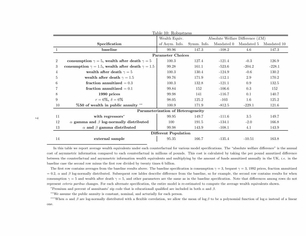
Table 10: RobustnessWealth Equiv. Absolute Welfare Difference (£M)

Specification of Asym. Info. Symm. Info. Mandated 0 Mandated 5 Mandated 10

1 baseline 99.96 147.3 -108.2 4.6 147.3

Parameter Choices

2 consumption γ = 5, wealth after death γ = 5 100.3 127.4 -121.4 -0.3 126.9

3 consumption γ = 1.5, wealth after death γ = 1.5 99.28 161.1 -523.6 -204.2 -228.1

4 wealth after death γ = 5 100.3 130.4 -124.9 -0.6 130.2

5 wealth after death γ = 1.5 99.76 171.9 -112.1 2.9 170.2

6 fraction annuitized = 0.3 100.3 132.8 -121.1 0.9 132.5

7 fraction annuitized = 0.1 99.84 152 -106.6 0.3 152

8 1990 prices 99.98 141 -116.7 0.1 140.7

9 r = 6%, δ = 6% 98.05 125.2 -103 1.6 125.2

10 %50 of wealth in public annuity ∗∗ 100.9 171.9 -812.5 -229.1 121.6

Parameterization of Heterogeneity

11 with regressors∗ 99.95 149.7 -111.6 3.5 149.7

12 α gamma and β log-normally distributed 100 191.5 -134.1 -2.0 166.8

13 α and β gamma distributed 99.98 143.9 -108.1 4.1 143.9

Different Population

14 external sample 95.35 166.7 -135.4 -10.51 163.8

In this table we report average wealth equivalents under each counterfactual for various model specifications. The “absolute welfare difference” is the annual

cost of asymmetric information compared to each counterfactual in millions of pounds. This cost is calculated by taking the per pound annutized difference

between the counterfactual and asymmetric information wealth equivalents and multiplying by the amount of funds annuitized annually in the UK, i.e. in the

baseline case the second row minus the first row divided by twenty times 6 billion.

The first row contains averages from the baseline results above. The baseline specification is consumption γ = 3, bequest γ = 3, 1992 prices, fraction annuitized

= 0.2, α and β log-normally distributed. Subsequent row lables describe difference from the baseline, so for example, the second row contains results for when

consumption γ = 5 and wealth after death γ = 5, and other parameters are the same as in the baseline specification. Note that differences among rows do not

represent ceteris paribus changes. For each alternate specification, the entire model is re-estimated to compute the average wealth equivalents shown.∗Premium and percent of annuitants’ zip code that is educationall qualified are included in both α and β.∗∗We assume the public annuity is constant, nominal, and acturially for each person.∗∗∗When α and β are log-normally distributed with a flexible correlation, we allow the mean of log β to be a polynomial function of log α instead of a linear

one.

7

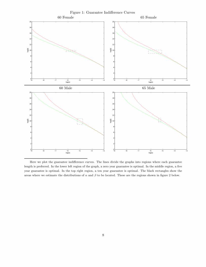
Figure 1: Guarantee Indifference Curves

60 Female 65 Female

−9 −8 −7 −6 −5 −4 −30

2

4

6

8

10

12

14

16

18

20

log(α)

log(

β)

−9 −8 −7 −6 −5 −4 −30

2

4

6

8

10

12

14

16

18

20

log(α)

log(

β)

60 Male 65 Male

−9 −8 −7 −6 −5 −4 −30

2

4

6

8

10

12

14

16

18

20

log(α)

log(

β)

−9 −8 −7 −6 −5 −4 −30

2

4

6

8

10

12

14

16

18

20

log(α)

log(

β)

Here we plot the guarantee indifference curves. The lines divide the graphs into regions where each guarantee

length is preferred. In the lower left region of the graph, a zero year guarantee is optimal. In the middle region, a five

year guarantee is optimal. In the top right region, a ten year guarantee is optimal. The black rectangles show the

areas where we estimate the distributions of α and β to be located. These are the regions shown in figure 2 below.

8

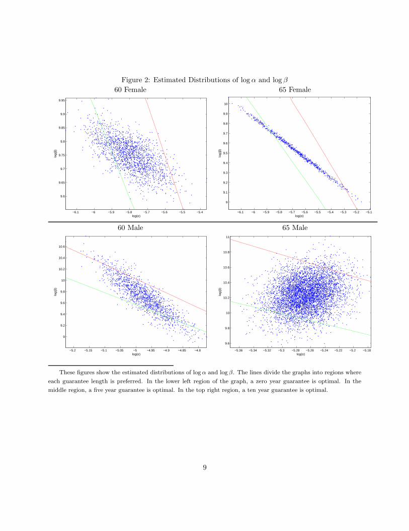
Figure 2: Estimated Distributions of log α and log β

60 Female 65 Female

−6.1 −6 −5.9 −5.8 −5.7 −5.6 −5.5 −5.4

9.6

9.65

9.7

9.75

9.8

9.85

9.9

9.95

log(α)

log(

β)

−6.1 −6 −5.9 −5.8 −5.7 −5.6 −5.5 −5.4 −5.3 −5.2 −5.1

9

9.1

9.2

9.3

9.4

9.5

9.6

9.7

9.8

9.9

10

log(α)lo

g(β)

60 Male 65 Male

−5.2 −5.15 −5.1 −5.05 −5 −4.95 −4.9 −4.85 −4.8

9

9.2

9.4

9.6

9.8

10

10.2

10.4

10.6

log(α)

log(

β)

−5.36 −5.34 −5.32 −5.3 −5.28 −5.26 −5.24 −5.22 −5.2 −5.18

9.6

9.8

10

10.2

10.4

10.6

10.8

11

log(α)

log(

β)

These figures show the estimated distributions of log α and log β. The lines divide the graphs into regions where

each guarantee length is preferred. In the lower left region of the graph, a zero year guarantee is optimal. In the

middle region, a five year guarantee is optimal. In the top right region, a ten year guarantee is optimal.

9

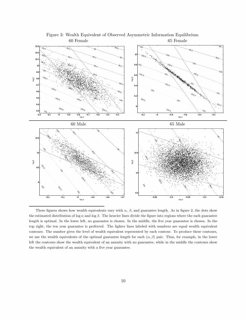
Figure 3: Wealth Equivalent of Observed Asymmetric Information Equilibrium

60 Female 65 Female

−6.2 −6.1 −6 −5.9 −5.8 −5.7 −5.6 −5.5 −5.4

9.3

9.4

9.5

9.6

9.7

9.8

9.9

10

10.1

10.2

10.3 98.899

99

99.2

99.2

99.2

99.4

99.4

99.4

99.6

99.6

99.6

99.6

99.8

99.8

99.8

99.8

100

100

100

100

100.2

100.2

100.2

100.4

100.4

100.4

100.6

100.6

100.8101

log α

log

β

−6.2 −6.1 −6 −5.9 −5.8 −5.7 −5.6 −5.5 −5.4

9.3

9.4

9.5

9.6

9.7

9.8

9.9

10

10.1

10.2

10.3

−6.2 −6 −5.8 −5.6 −5.4 −5.2

9

9.2

9.4

9.6

9.8

10

99

99.5

99.5

100

100

100

100

100.5

100.5

100.5

101

101

101

101

101.5

101.5

101.5

101.5

102

102

102

102.5

102.5

log α

log

β

−6.2 −6 −5.8 −5.6 −5.4 −5.2

9

9.2

9.4

9.6

9.8

10

60 Male 65 Male

−5.2 −5.1 −5 −4.9 −4.8 −4.7

9

9.5

10

10.5

99

99

99.5

99.5

99.5

100

100

100

100

100.5

100.5

100.5

101

101

101

101.5

101.5102

log α

log

β

−5.2 −5.1 −5 −4.9 −4.8 −4.7

9

9.5

10

10.5

−5.35 −5.3 −5.25 −5.2 −5.15

9.5

10

10.5

11

99

99.5

99.5

99.5

100

100

100

100.5

100.5

101

log α

log

β

−5.35 −5.3 −5.25 −5.2 −5.15

9.5

10

10.5

11

These figures shows how wealth equivalents vary with α, β, and guarantee length. As in figure 2, the dots show

the estimated distribution of log α and log β. The heavier lines divide the figure into regions where the each guarantee

length is optimal. In the lower left, no guarantee is chosen. In the middle, the five year guarantee is chosen. In the

top right, the ten year guarantee is preferred. The lighter lines labeled with numbers are equal wealth equivalent

contours. The number gives the level of wealth equivalent represented by each contour. To produce these contours,

we use the wealth equivalents of the optimal guarantee length for each (α, β) pair. Thus, for example, in the lower

left the contours show the wealth equivalent of an annuity with no guarantee, while in the middle the contours show

the wealth equivalent of an annuity with a five year guarantee.

10

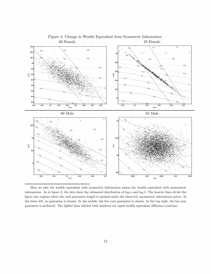
Figure 4: Change in Wealth Equivalent from Symmetric Information

60 Female 65 Female

−6.2 −6.1 −6 −5.9 −5.8 −5.7 −5.6 −5.5 −5.4

9.3

9.4

9.5

9.6

9.7

9.8

9.9

10

10.1

10.2

10.3

−0.4

−0.4

−0.2

−0.2

−0.2

0

0

0

0

0.20.2

0.2

0.40.4 0.4

0.60.6 0.6

0.8 0.8 0.8

log α

log

β

−6.2 −6.1 −6 −5.9 −5.8 −5.7 −5.6 −5.5 −5.4

9.3

9.4

9.5

9.6

9.7

9.8

9.9

10

10.1

10.2

10.3

−6.2 −6 −5.8 −5.6 −5.4 −5.2

9

9.2

9.4

9.6

9.8

10

−0.8

−0.8 −0.6

−0.6

−0.6

−0.4

−0.4

−0.4

−0.2

−0.2

−0.2

0

0

0

0

0.2

0.2

0.2

0.4

0.4

0.4

0.6

0.6 0.6

0.8

0.8 0.8

11 1 1

1.2 1.2 1.2

log α

log

β

−6.2 −6 −5.8 −5.6 −5.4 −5.2

9

9.2

9.4

9.6

9.8

10

60 Male 65 Male

−5.2 −5.1 −5 −4.9 −4.8 −4.7

9

9.5

10

10.5

−0.8 −0.6

−0.6

−0.4

−0.4

−0.2

−0.2

−0.2

0

0

0

0

0.2

0.2

0.2

0.2

0.4

0.4

0.4

0.4

0.6

0.6

0.6 0.6

0.8

0.80.8

11

1

log α

log

β

−5.2 −5.1 −5 −4.9 −4.8 −4.7

9

9.5

10

10.5

−5.35 −5.3 −5.25 −5.2 −5.15

9.5

10

10.5

11

00.2

0.2

0.4

0.4

0.4

0.6

0.6

0.6

0.6

0.8

0.8

0.80.8

1

1

1

log α

log

β

−5.35 −5.3 −5.25 −5.2 −5.15

9.5

10

10.5

11

Here we plot the wealth equivalent with symmetric information minus the wealth equivalent with asymmetric

information. As in figure 2, the dots show the estimated distribution of log α and log β. The heavier lines divide the

figure into regions where the each guarantee length is optimal under the observed, asymmetric information prices. In

the lower left, no guarantee is chosen. In the middle, the five year guarantee is chosen. In the top right, the ten year

guarantee is preferred. The lighter lines labeled with numbers are equal wealth equivalent difference contours.

11

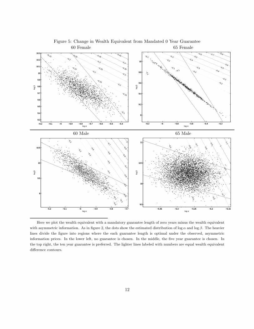
Figure 5: Change in Wealth Equivalent from Mandated 0 Year Guarantee

60 Female 65 Female

−6.2 −6.1 −6 −5.9 −5.8 −5.7 −5.6 −5.5 −5.4

9.3

9.4

9.5

9.6

9.7

9.8

9.9

10

10.1

10.2

10.3 −0.45

−0.4

−0.35

−0.35

−0.3

−0.3

−0.25

−0.25

−0.2

−0.2

−0.2

−0.15

−0.15

−0.15

−0.15

−0.1

−0.1

−0.1

−0.1

log α

log

β

−6.2 −6.1 −6 −5.9 −5.8 −5.7 −5.6 −5.5 −5.4

9.3

9.4

9.5

9.6

9.7

9.8

9.9

10

10.1

10.2

10.3

−6.2 −6 −5.8 −5.6 −5.4 −5.2

9

9.2

9.4

9.6

9.8

10

−0.8−0.7−0.6

−0.6

−0.5

−0.5

−0.4

−0.4

−0.3

−0.3

−0.3

−0.2

−0.2

−0.2

−0.1

−0.1

−0.1

−0.1

−0.1

log α

log

β

−6.2 −6 −5.8 −5.6 −5.4 −5.2

9

9.2

9.4

9.6

9.8

10

60 Male 65 Male

−5.2 −5.1 −5 −4.9 −4.8 −4.7

9

9.5

10

10.5

−1

−0.9−0.8

−0.7

−0.7

−0.6

−0.6

−0.5

−0.5

−0.4

−0.4

−0.4

−0.3

−0.3

−0.3−0.3−0.3

−0.3

−0.2

−0.2

log α

log

β

−5.2 −5.1 −5 −4.9 −4.8 −4.7

9

9.5

10

10.5

−5.35 −5.3 −5.25 −5.2 −5.15

9.5

10

10.5

11

−1.1

−1

−0.9

−0.9

−0.8

−0.8

−0.7

−0.7

−0.7

−0.6

−0.6

−0.6

−0.5

−0.5

−0.5

log α

log

β

−5.35 −5.3 −5.25 −5.2 −5.15

9.5

10

10.5

11

Here we plot the wealth equivalent with a mandatory guarantee length of zero years minus the wealth equivalent

with asymmetric information. As in figure 2, the dots show the estimated distribution of log α and log β. The heavier

lines divide the figure into regions where the each guarantee length is optimal under the observed, asymmetric

information prices. In the lower left, no guarantee is chosen. In the middle, the five year guarantee is chosen. In

the top right, the ten year guarantee is preferred. The lighter lines labeled with numbers are equal wealth equivalent

difference contours.

12

Figure 6: Change in Wealth Equivalent from Mandated 5 Year Guarantee

60 Female 65 Female

−6.2 −6.1 −6 −5.9 −5.8 −5.7 −5.6 −5.5 −5.4

9.3

9.4

9.5

9.6

9.7

9.8

9.9

10

10.1

10.2

10.3−0.2

−0.15

−0.1

−0.1

−0.05

−0.05

−0.05

−0.05

0

0

0

0

0

0

0

log α

log

β

−6.2 −6.1 −6 −5.9 −5.8 −5.7 −5.6 −5.5 −5.4

9.3

9.4

9.5

9.6

9.7

9.8

9.9

10

10.1

10.2

10.3

−6.2 −6 −5.8 −5.6 −5.4 −5.2

9

9.2

9.4

9.6

9.8

10

−0.35−0.3−0.25

−0.2

−0.2

−0.15

−0.15

−0.15

−0.1

−0.1

−0.1

−0.1

−0.05

−0.05

−0.05

−0.05

−0.05

−0.05

0

0

00

0

0

0

0.05

0.05

0.05

0.05

0.05

0.05

0.05

0.1

0.1

0.1

0.1

0.1

0.1

0.1

0.1

log α

log

β

−6.2 −6 −5.8 −5.6 −5.4 −5.2

9

9.2

9.4

9.6

9.8

10

60 Male 65 Male

−5.2 −5.1 −5 −4.9 −4.8 −4.7

9

9.5

10

10.5

−0.35−0.3

−0.25

−0.2

−0.2

−0.2

−0.15

−0.15

−0.15

−0.15

−0.1

−0.1

−0.1

−0.1

−0.1

−0.05

−0.05

−0.05−0.05

−0.05

−0.05

0

0

0

0

0

0

0

0.05

0.05

0.05

0.05

0.05

0.05

0.05

0.1

0.1

0.1

log α

log

β

−5.2 −5.1 −5 −4.9 −4.8 −4.7

9

9.5

10

10.5

−5.35 −5.3 −5.25 −5.2 −5.15

9.5

10

10.5

11

−0.3−0.25

−0.2

−0.2

−0.15

−0.15

−0.15

−0.1

−0.1

−0.1

−0.1

−0.1

−0.05

−0.05

−0.05

−0.05

−0.05

−0.05

0

0

0

0

0

0

log α

log

β

−5.35 −5.3 −5.25 −5.2 −5.15

9.5

10

10.5

11

Here we plot the wealth equivalent with a mandatory guarantee length of five years minus the wealth equivalent

with asymmetric information. As in figure 2, the dots show the estimated distribution of log α and log β. The heavier

lines divide the figure into regions where the each guarantee length is optimal under the observed, asymmetric

information prices. In the lower left, no guarantee is chosen. In the middle, the five year guarantee is chosen. In

the top right, the ten year guarantee is preferred. The lighter lines labeled with numbers are equal wealth equivalent

difference contours.

13

Figure 7: Change in Wealth Equivalent from Mandated 10 Year Guarantee

60 Female 65 Female

−6.2 −6.1 −6 −5.9 −5.8 −5.7 −5.6 −5.5 −5.4

9.3

9.4

9.5

9.6

9.7

9.8

9.9

10

10.1

10.2

10.3

−0.05 0

0

0.05

0.05

0.05

0.1

0.1

0.1

0.15

0.15

0.15

0.15

0.2

0.2

0.2

0.2

log α

log

β

−6.2 −6.1 −6 −5.9 −5.8 −5.7 −5.6 −5.5 −5.4

9.3

9.4

9.5

9.6

9.7

9.8

9.9

10

10.1

10.2

10.3

−6.2 −6 −5.8 −5.6 −5.4 −5.2

9

9.2

9.4

9.6

9.8

10

−0.3

−0.2

−0.2

−0.1

−0.1

−0.1

0

0

0

0

0.1

0.1

0.1

0.1

0.2

0.2

0.2

0.2

0.3

0.3

0.3

0.3

log α

log

β

−6.2 −6 −5.8 −5.6 −5.4 −5.2

9

9.2

9.4

9.6

9.8

10

60 Male 65 Male

−5.2 −5.1 −5 −4.9 −4.8 −4.7

9

9.5

10

10.5

−0.3

−0.2

−0.2

−0.1

−0.1

0

0

0

0.1

0.1

0.1

0.2

0.2

0.2

0.3

0.3

0.3

0.4

0.4

0.4

log α

log

β

−5.2 −5.1 −5 −4.9 −4.8 −4.7

9

9.5

10

10.5

−5.35 −5.3 −5.25 −5.2 −5.15

9.5

10

10.5

11

0.10.2

0.3

0.3

0.4

0.4

0.4

0.5

0.5

0.5

0.6

0.6

0.6

0.7

0.7

0.7

0.8

0.8

0.8

0.8

0.8

log α

log

β

−5.35 −5.3 −5.25 −5.2 −5.15

9.5

10

10.5

11

Here we plot the wealth equivalent with a mandatory guarantee length of ten years minus the wealth equivalent

with asymmetric information. As in figure 2, the dots show the estimated distribution of log α and log β. The heavier

lines divide the figure into regions where the each guarantee length is optimal under the observed, asymmetric

information prices. In the lower left, no guarantee is chosen. In the middle, the five year guarantee is chosen. In

the top right, the ten year guarantee is preferred. The lighter lines labeled with numbers are equal wealth equivalent

difference contours.

14