Research assistance from Augustine Denteh is much appreciated, and the authors thank Julie Cullen and Raj Chetty for making programs used to estimate unemployment insurance benefits available. They also thank James Alm, Kelly Chen, Andrew Friedson, Mei Dong, Tim Dunne, Kelsey O’Connor, Andrew Oswald, John Robertson, Ling Sun, and Randall Wright for helpful comments and suggestions. The views expressed here are the authors’ and not necessarily those of the Federal Reserve Bank of Atlanta or the Federal Reserve System. Any remaining errors are the authors’ responsibility. Please address questions regarding content to Julie L. Hotchkiss, Research Department, Federal Reserve Bank of Atlanta, 1000 Peachtree Street NE, Atlanta, GA 30309-4470, 404-498-8198, Julie.L.Hotchkiss@atl.frb.org; Robert E. Moore, Office of the Dean, Department of Economics, Andrew Young School of Policy Studies, Georgia State University, P.O. Box 3992, Atlanta, GA 30302-3992, rmoore@gsu.edu; or Fernando Rios-Avila, Levy Economics Institute of Bard College, Blithewood, Annandale-on-Hudson, NY 12504-5000, friosavi@levy.org. Federal Reserve Bank of Atlanta working papers, including revised versions, are available on the Atlanta Fed’s website at www.frbatlanta.org. Click “Publications” and then “Working Papers.” To receive e-mail notifications about new papers, use frbatlanta.org/forms/subscribe.

FEDERAL RESERVE BANK of ATLANTA WORKING PAPER SERIES

Family Welfare and the Cost of Unemployment Julie L. Hotchkiss, Robert E. Moore, and Fernando Rios-Avila Working Paper 2017-7 September 2017 Abstract: This paper calculates the cost of an unemployment shock in terms of family welfare for married and single families separately and by education level. We find that, overall, families face an average annualized expected dollar equivalent welfare loss of $1,156 when the unemployment rate rises by 1 percentage point. The average welfare loss for married families is greater than the average loss for single families and increases in education. We then estimate that a price level increase of 1.8 percent generates the same amount of welfare loss. We also find that the average welfare loss from a shock to prices versus a shock to unemployment rises with income. JEL classification: I30, E52, J22, D19 Key words: family welfare, joint labor supply, microsimulation dual mandate, monetary policy

- 1 -

Family Welfare and the Cost of Unemployment 1 Introduction and Background

The purpose of this paper is to evaluate the welfare cost of a shock to unemployment for

families with different characteristics. We apply the microsimulation methodology used by

(Hotchkiss, Moore, and Rios-Avila 2012; Hotchkiss et al. 2017), and others, to estimate

parameters of a labor supply model within the context of a family utility framework for married

couple households, and within the context of a unitary utility framework for single households.1

Estimated parameters from the utility model will be used to simulate the expected welfare loss

from a rise in the aggregate unemployment rate, with the recognition that each person's

probability of unemployment is impacted differently by a softening of the labor market.

Others have explored the costs of unemployment almost exclusively through a

macroeconomic lens. Okun's Law (Okun 1962) is often used to describe the loss in output that is

generated from an additional one-percentage point rise in the unemployment rate. Gordon,

Nordhaus, and Poole (1973) detail the deficiencies of Okun's Law (alone) for measuring the

welfare effects of a rise in the unemployment rate because the relationship does not account for

the value of non-market activity. And rather than explore the cost of a specific shock to

unemployment, some focus more on the welfare costs of economic volatility (e.g. Lucas 1991;

Krusell and Smith 1999).

An exception to the macroeconomic approach to measuring the welfare costs of

unemployment is found in Hurd (1980). Hurd uses estimated individual labor supply elasticities

(or, rather, the slope of the labor supply function) to calculate the payment required to make a

person indifferent between working the desired hours at a prevailing wage rate, or being forced

1 Microsimulation is a popular methodology for assessing the impact of policy changes on welfare (for example, see Fiorio 2008; Blundell et al. 2000; Bahl et al. 1993; Blundell 1992).

- 2 -

to work fewer hours than desired because of unemployment. This payment is interpreted as the

cost of unemployment. Our methodology employs a similar, but more complete, strategy in that

we estimate the welfare loss of deviating from desired hours, but we estimate utility function

parameters in order to calculate actual loss in welfare (i.e., utility) as opposed to just loss in

income that would come from unemployment. Among other things, this allows us to account for

any potential welfare gain from an increase in non-market activity that comes with non-

employment. The methodology also allows a comparison of welfare loss across families of

different characteristics irrespective of the actual utility level of those families (either

independently or relative to one another).

DiTella, MacCulloch, and Oswald (2001) also offer an estimate of the utility-constant

cost of unemployment and provide a segue to the second part of the analysis in this paper. They

assess the relative importance of high unemployment vs. high inflation in explaining variations

in demographic-neutral aggregate levels of satisfaction across countries and time. They find that

unemployment is more important than inflation in reducing overall satisfaction. They motivate

their analysis by stating that, "... reducing inflation is often costly, in terms of extra

unemployment...," (DiTella, MacCulloch, and Oswald 2001, 335). This trade-off is also

acknowledged by Gordon, Nordhaus, and Poole (1973) as a motivation for undertaking their

assessment of the welfare cost of higher unemployment. However, they note that their

assessment will not take account of, "...the benefits associated with the lower inflation rate made

possible by higher unemployment," (p. 135).2

The potential trade-off between unemployment and inflation suggested by these papers is

2 In spite of this implied negative relationship between unemployment and inflation, Berentsen, Menzio, and Wright (2011) identify a positive relationship between unemployment and inflation in very low frequency data (the long run).

- 3 -

of particular interest to U.S. Federal Reserve monetary policy makers whose actions are guided

by what is know as the "Dual Mandate" of full employment and stable prices, which is spelled

out in Section 2A of the Federal Reserve Act:

“The Board of Governors of the Federal Reserve System and the Federal Open Market Committee shall maintain long run growth of the monetary and credit aggregates commensurate with the economy’s long run potential to increase production, so as to promote effectively the goals of maximum employment, stable prices, and moderate long-term interest rates.” 3

While we do not model inflation, per se, in this paper, the second part of our analysis makes use

of the microsimulation to also estimate the size of an unanticipated shock to prices that would

generate the same welfare loss as a one percentage-point shock to unemployment. Since the only

consumption price in the model is the numeraire price of consumption, we simulate a price shock

by adjusting the value of the other components of the model that enter in real dollars -- wages

and non-labor income. We will then be able to say something about how the individual family

views the trade off between rising unemployment and rising prices. To the extent that the Fed is

concerned with the distributional implications of monetary policy, such as income inequality

(e.g., Bernanke 2015; Nakajima 2015; Amaral 2017), how the welfare cost of unemployment and

price level changes differs across demographic characteristics may also be of interest to

monetary policy makers.

We find that the annualized expected welfare loss generated by a one-percentage point

shock to the unemployment rate is equivalent to $1,156, on average across all families. And even

though the probability of unemployment is less for those with higher education, their potential

income loss is greater, making the expected welfare loss for those with higher education greater

than for those with less education. In addition, single families' expected loss is less than that of

married families. This lower expected loss for singles translates into a lower equivalent

3 See http://www.federalreserve.gov/aboutthefed/fract.htm.

- 4 -

unanticipated price level increase for singles than for married families; single families are only

willing to tolerate a smaller increase in prices to avoid unemployment than married families are.

This result is consistent with the conclusions of Burdett et al. (2016), who find that inflation is

more costly for singles because, "...being single is cash intensive" (p. 337); also see Dong, Sun,

and Wright (2015).

2 Methodology

The main advantage to the theoretical framework we employ for this exercise is that it is

constructed from a standard joint (unitary for singles) family utility model. For married couples,

labor supply is jointly estimated. The utility function does not include unemployment as a direct

input in the optimization problem.4 However, changes in unemployment and prices can be

brought to bear on the welfare outcome by simulating the impact these environmental changes

have on behavior and family utility

2.1 Family Utility Framework

The model described in this section nests the more simple case of single households.

Empirically, the single family version of the model implies constraining hours and wages of the

second household member to zero, as well as constraining all utility parameters concerning the

second member to be zero.

Family labor supply decisions are modeled in a neoclassical joint utility framework. This

model can be thought of as a reduced-form specification of family decision-making. The model

yields a clear-cut expression of family welfare that allows for cross wage effects on each

member's labor supply decision. The assumption of joint family utility (or, "collective" utility) is

4 In spite of the insistence by Hall (1981, 432) that, "inflation is an outcome of economic processes, not an exogenous causal influence," it is certainly exogenous to an individual family's decision making process.

- 5 -

often rejected in favor of a bargaining structure for modeling intra-familial decisions making (for

example, see Apps and Rees 2009; McElroy 1990). However, there is evidence that the choice of

structure for household decision making has very little implication for conclusions in

microsimulation exercises (see Moreau and Bargain 2005). In addition, Blundell et al. (2007)

find that both collective and bargaining models are consistent with their household labor supply

model estimated in the U.K.

Within the framework of the neoclassical family labor supply model, a family maximizes

a utility function that represents household welfare. Assuming, for simplicity, that there are only

two working members of the household (husband and wife), the family chooses levels of non-

market time (e.g., leisure, household production) for each member and a joint consumption level

in order to solve the following problem:5

max!!,!!,!

𝑈 = 𝑈 𝐿!, 𝐿!,𝐶  

𝑠𝑢𝑏𝑗𝑒𝑐𝑡  𝑡𝑜  𝐶 = 𝑤!ℎ! + 𝑤!ℎ! + 𝑌 . (1) Define T as total time available for an individual; 𝐿! = 𝑇 − ℎ! will be referred to as the

husband's non-market time, and 𝐿! = 𝑇 − ℎ! will be referred to as the wife's non-market time;

ℎ! is the labor supply of the husband; ℎ! is the labor supply of the wife; C is total money income

(or consumption with price equal to one); 𝑤! and 𝑤! are the husband's and wife's after-tax

market wage, respectively; and Y is non-labor income. 𝐿! and 𝐿! correspond to all uses of non-

market time, including home production activities.6 In addition, the model does not distinguish

5 Sample construction excludes families with unmarried, same- or opposite-sex adults/partners. There are not enough occurrences to produce reliable utility function parameters for this family type. This exclusion also ensures a clean interpretation of individual family members' contributions to leisure/household production and total consumption. 6 Apps and Rees (2009) are highly critical of family utility models that do not include measures of household production, but even they acknowledge that not much can be done without the availability of richer data (p. 108). Since the focus of the analysis in this paper is utility at the household level, the absence of home production activities is not crucial.

- 6 -

between unemployment and non-participation; both states are included in the non-employment

status. The implications of this are discussed later in section 2.3.

The solution to the maximization problem in equation (1) can be expressed in terms of

the indirect utility function, which is solely a function of the wages of the husband and wife and

non-labor income of the family:

𝑉 𝑤!,𝑤!,𝑌 = 𝑈 𝑇 − ℎ!∗ 𝑤!,𝑤!,𝑌 , 𝑇 − ℎ!∗ 𝑤!,𝑤!,𝑌 ,

                                                                    𝑤!ℎ!∗ 𝑤!,𝑤!,𝑌 + 𝑤!ℎ!∗ 𝑤!,𝑤!,𝑌 + 𝑌 , (2)

where ℎ!∗ 𝑤!,𝑤!,𝑌 and ℎ!∗ 𝑤!,𝑤!,𝑌 correspond to the optimal labor supply equations (desired

hours) for the husband and wife, respectively. By totally differentiating the indirect utility

function, we can simulate the change in welfare that results from changes in optimal hours of

work and consumption in response to changes in wages and non-labor income (also see Apps

and Rees 2009, 263):

𝑑𝑉 = −𝑈!𝑑ℎ!∗ − 𝑈!𝑑ℎ!∗ + 𝑈!𝑑𝐶∗ , (3)

where 𝑈! and 𝑈! are the family's marginal utility of the husband's and wife's non-market time,

respectively, and 𝑈! is the family's marginal utility of consumption. It is this equation that gives

us the change in family welfare that will result from a shock to unemployment or a shock to

prices. It is clear from equation (3) that the change in welfare not only depends on the individual

labor supply responses, but also on the family's marginal evaluation of a change in non-market

time and income.

2.2 Estimation of Utility Function Parameters and Labor Supply Elasticities

Simulating the impact on family welfare of higher unemployment and an unanticipated

shock to prices requires the estimation of labor supply elasticities of each family member with

respect to changes in their own and each other's (in the case of married-couple families) wages,

- 7 -

elasticities with respect to non-labor family income, as well as the changes in the probability of

employment (extensive margin elasticities); i.e., the probability of being at an interior solution on

the budget constraint. There are many divergent empirical issues raised in the literature related to

estimating labor supply elasticities. While the focus of this paper is on the simulation exercise

itself, the simulation does require labor supply elasticities and it is, therefore, worthwhile to

address some of the empirical issues; most of these issues, including the potential for

endogeneity of wages and non-labor income, are addressed in detail in Appendix A. The goal

here is to produce reasonable labor supply elasticities that are consistent with the literature.

Toward that end, the methodology adopted takes the simplest approach possible while

maintaining basic theoretical and empirical integrity.

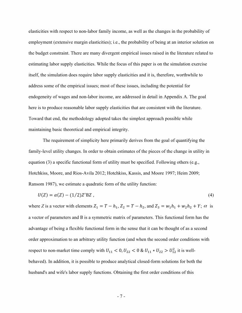
The requirement of simplicity here primarily derives from the goal of quantifying the

family-level utility changes. In order to obtain estimates of the pieces of the change in utility in

equation (3) a specific functional form of utility must be specified. Following others (e.g.,

Hotchkiss, Moore, and Rios-Avila 2012; Hotchkiss, Kassis, and Moore 1997; Heim 2009;

Ransom 1987), we estimate a quadratic form of the utility function:

   𝑈 𝑍 = 𝛼 𝑍 − (1 2)𝑍!Β𝑍 , (4)

where Z is a vector with elements 𝑍! = 𝑇 − ℎ!, 𝑍! = 𝑇 − ℎ!, and 𝑍! = 𝑤!ℎ! + 𝑤!ℎ! + 𝑌; is

a vector of parameters and Β is a symmetric matrix of parameters. This functional form has the

advantage of being a flexible functional form in the sense that it can be thought of as a second

order approximation to an arbitrary utility function (and when the second order conditions with

respect to non-market time comply with 𝑈!! < 0,𝑈!! < 0  &  𝑈!! ∗ 𝑈!! > 𝑈!"! it is well-

behaved). In addition, it is possible to produce analytical closed-form solutions for both the

husband's and wife's labor supply functions. Obtaining the first order conditions of this

α

- 8 -

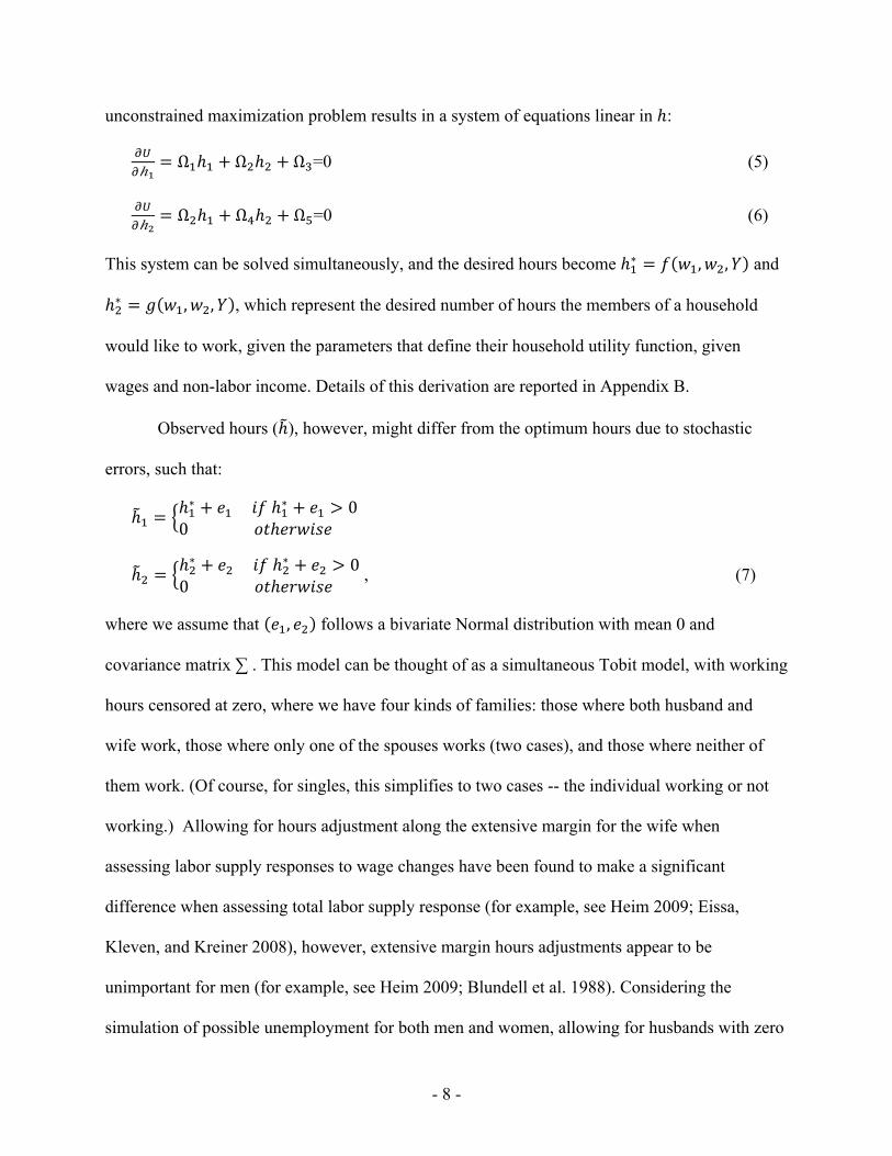
unconstrained maximization problem results in a system of equations linear in ℎ:

!!!ℎ!

= Ω!ℎ! + Ω!ℎ! + Ω!=0 (5)

!!!ℎ!

= Ω!ℎ! + Ω!ℎ! + Ω!=0 (6)

This system can be solved simultaneously, and the desired hours become ℎ!∗ = 𝑓 𝑤!,𝑤!,𝑌 and

ℎ!∗ = 𝑔 𝑤!,𝑤!,𝑌 , which represent the desired number of hours the members of a household

would like to work, given the parameters that define their household utility function, given

wages and non-labor income. Details of this derivation are reported in Appendix B.

Observed hours (ℎ), however, might differ from the optimum hours due to stochastic

errors, such that:

ℎ! =ℎ!∗ + 𝑒!          𝑖𝑓  ℎ!∗ + 𝑒! > 00                                  𝑜𝑡ℎ𝑒𝑟𝑤𝑖𝑠𝑒

 

ℎ! =ℎ!∗ + 𝑒!          𝑖𝑓  ℎ!∗ + 𝑒! > 00                                  𝑜𝑡ℎ𝑒𝑟𝑤𝑖𝑠𝑒

, (7)

where we assume that 𝑒!, 𝑒! follows a bivariate Normal distribution with mean 0 and

covariance matrix ∑ . This model can be thought of as a simultaneous Tobit model, with working

hours censored at zero, where we have four kinds of families: those where both husband and

wife work, those where only one of the spouses works (two cases), and those where neither of

them work. (Of course, for singles, this simplifies to two cases -- the individual working or not

working.) Allowing for hours adjustment along the extensive margin for the wife when

assessing labor supply responses to wage changes have been found to make a significant

difference when assessing total labor supply response (for example, see Heim 2009; Eissa,

Kleven, and Kreiner 2008), however, extensive margin hours adjustments appear to be

unimportant for men (for example, see Heim 2009; Blundell et al. 1988). Considering the

simulation of possible unemployment for both men and women, allowing for husbands with zero

- 9 -

hours of work is important, so they will be included in the analysis.

Allowing for the presence of non-workers raises one empirical issue identified by Keane

(2011) that must be addressed: market wages are not observed for individuals who do not work.

To obtain estimates of those wages, we take the standard approach in the literature of estimating

a selectivity-corrected wage equation (Heckman 1974) using regressors observable for both

working and non-working individuals.7 The resulting parameter estimates are then used to

predict wages for non-working men and women based on their observable characteristics.

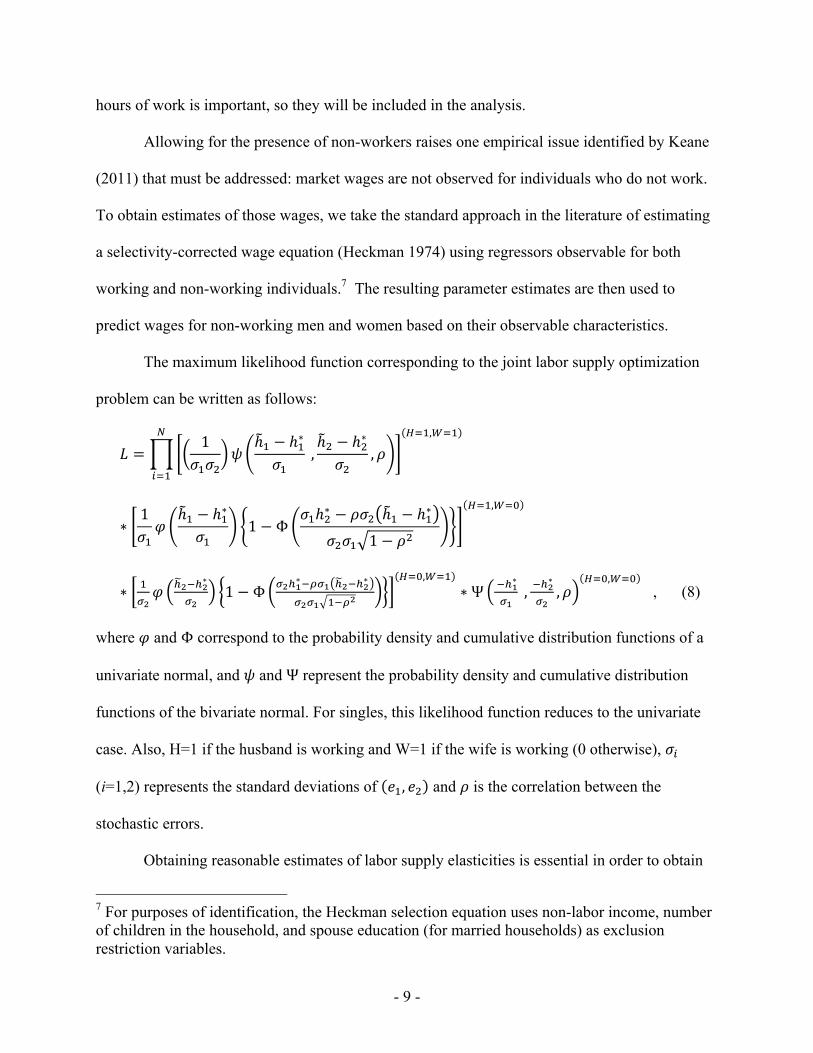
The maximum likelihood function corresponding to the joint labor supply optimization

problem can be written as follows:

𝐿 =1

𝜎!𝜎!𝜓

ℎ! − ℎ!∗

𝜎!   ,ℎ! − ℎ!∗

𝜎!,𝜌

!!!,!!!!

!!!

∗1𝜎!𝜑

ℎ! − ℎ!∗

𝜎!1−Φ

𝜎!ℎ!∗ − 𝜌𝜎! ℎ! − ℎ!∗

𝜎!𝜎! 1− 𝜌!

!!!,!!!

∗ !!!𝜑 !!!!!∗

!!1−Φ !!!!∗!!!! !!!!!∗

!!!! !!!!

!!!,!!!∗Ψ  !!!∗

!!   ,  !!!

∗

!!,𝜌

!!!,!!!   , (8)

where 𝜑 and Φ correspond to the probability density and cumulative distribution functions of a

univariate normal, and 𝜓 and Ψ represent the probability density and cumulative distribution

functions of the bivariate normal. For singles, this likelihood function reduces to the univariate

case. Also, H=1 if the husband is working and W=1 if the wife is working (0 otherwise), 𝜎!

(i=1,2) represents the standard deviations of 𝑒!, 𝑒! and 𝜌 is the correlation between the

stochastic errors.

Obtaining reasonable estimates of labor supply elasticities is essential in order to obtain

7 For purposes of identification, the Heckman selection equation uses non-labor income, number of children in the household, and spouse education (for married households) as exclusion restriction variables.

- 10 -

believable estimates of the change in utility through the simulation exercise described below.

Issues, well known to the literature, related to the estimation of labor supply elasticities and the

implications of those issues to the problem at hand are addressed in detail in Appendix A.

With the expectation of heterogeneity in preferences across families, particularly of

different income levels, we estimate different sets of parameters for families based on husband

education level for married couples, and head of the household education for single families. In

addition, we estimate different sets of parameters for male and female singles. In other words, we

estimate five sets of parameters for married families (full sample; and husband's education is less

than high school, high school, some college, and college plus) and 10 sets of parameters for

singles (full sample for men and women separately; then for each education level separately for

men and women).8

2.3 Expected Welfare Loss from a Shock to Aggregate Unemployment

We simulate a rise in the unemployment rate through an exogenous shock to the

stochastic errors in equation (7). If, for example, an employed husband loses his job, then

𝑒! = −ℎ!∗. This also implies that the estimated welfare impact of unemployment is, by

construction, zero if neither of the spouses is working.

The probability of each family member being hit by unemployment (or, rather, non-

employment, or losing a job) is a function of his or her demographic characteristics (gender,

race, age, and education). 9 If the marginal effect on the probability that the husband becomes

non-employed when the aggregate unemployment rate rises by one-percentage point is 𝑝! and

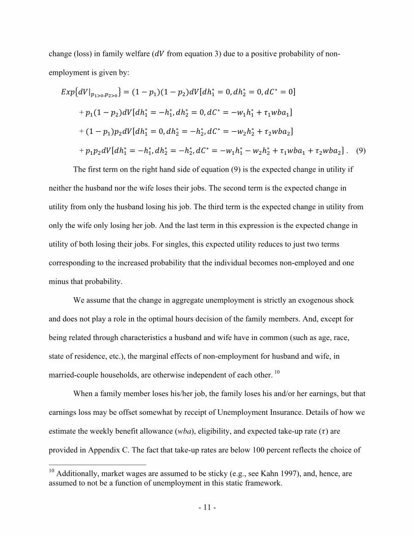
the marginal effect on the wife's probability becoming non-employed is 𝑝!, then the expected

8 There are many other dimensions across which utility function parameters could vary. We expect that differences across marital status and education/income would be most pronounced. 9 Note that our model does not distinguish between unemployment and out of the labor force -- there is only employment and non-employment.

- 11 -

change (loss) in family welfare (𝑑𝑉 from equation 3) due to a positive probability of non-

employment is given by:

𝐸𝑥𝑝 𝑑𝑉 !!!!,!!!! = (1− 𝑝!)(1− 𝑝!)𝑑𝑉 𝑑ℎ!∗ = 0,𝑑ℎ!∗ = 0,𝑑𝐶∗ = 0

+  𝑝!(1− 𝑝!)𝑑𝑉 𝑑ℎ!∗ = −ℎ!∗ ,𝑑ℎ!∗ = 0,𝑑𝐶∗ = −𝑤!ℎ!∗ + 𝜏!𝑤𝑏𝑎!

+  (1− 𝑝!)𝑝!𝑑𝑉 𝑑ℎ!∗ = 0,𝑑ℎ!∗ = −ℎ!∗ ,𝑑𝐶∗ = −𝑤!ℎ!∗ + 𝜏!𝑤𝑏𝑎!

+  𝑝!𝑝!𝑑𝑉 𝑑ℎ!∗ = −ℎ!∗ ,𝑑ℎ!∗ = −ℎ!∗ ,𝑑𝐶∗ = −𝑤!ℎ!∗ − 𝑤!ℎ!∗ + 𝜏!𝑤𝑏𝑎! + 𝜏!𝑤𝑏𝑎! . (9)

The first term on the right hand side of equation (9) is the expected change in utility if

neither the husband nor the wife loses their jobs. The second term is the expected change in

utility from only the husband losing his job. The third term is the expected change in utility from

only the wife only losing her job. And the last term in this expression is the expected change in

utility of both losing their jobs. For singles, this expected utility reduces to just two terms

corresponding to the increased probability that the individual becomes non-employed and one

minus that probability.

We assume that the change in aggregate unemployment is strictly an exogenous shock

and does not play a role in the optimal hours decision of the family members. And, except for

being related through characteristics a husband and wife have in common (such as age, race,

state of residence, etc.), the marginal effects of non-employment for husband and wife, in

married-couple households, are otherwise independent of each other. 10

When a family member loses his/her job, the family loses his and/or her earnings, but that

earnings loss may be offset somewhat by receipt of Unemployment Insurance. Details of how we

estimate the weekly benefit allowance (wba), eligibility, and expected take-up rate (𝜏) are

provided in Appendix C. The fact that take-up rates are below 100 percent reflects the choice of

10 Additionally, market wages are assumed to be sticky (e.g., see Kahn 1997), and, hence, are assumed to not be a function of unemployment in this static framework.

- 12 -

some individuals who lose their jobs to exit the labor force, rather than remain unemployed. The

family may also be able to offset earnings loss through previous savings. However, given that 63

percent of Americans say that they do not have enough savings to face an unexpected expense of

$500 to $1,000 (Picchi 2016; also see Trubey 2016), the absence of savings from our model is

not likely to bias our estimates of the expected loss in consumption.

The increases in the probabilities of non-employment are determined as follows.11 Each

person is assigned to one of 64 specific demographic groups (based on two gender, two race,

four age, and four education classifications). The impact of a rise in the state/year aggregate

unemployment rate on the probability of non-employment for a member of that group is

determined by 64 time-series probit estimations using observations from the March supplement

of the Current Population Survey from the time period 2003-2013 with year and state fixed-

effects. For example, the smallest marginal effect of a one-percentage point increase in the

aggregate unemployment rate was estimated to be a 0.056 percentage point decline in

employment for white women, between 35 and 44 years old, with at least a college degree.

Therefore, 𝑝! for a woman with these characteristics is set equal to 0.00056. The largest impact

was estimated to be a 2.4 percentage point employment decline for white men, between the ages

of 18 and 34, with less than a high school degree. Therefore, 𝑝! for a man with this set of

characteristics is set equal to 0.024.12 Given a set of estimated utility function parameters, and

estimated probabilities of non-employment, then, the family-specific impact on expected utility

of a one-percentage point rise in the unemployment rate is given by equation (9).

11 This procedure is similar to that employed by Gramlich (1974) in his assessment of the distributional consequences of unemployment. 12 The full spectrum of non-employment marginal effects across the 64 demographic groups is available upon request.

- 13 -

The model does not explicitly depend on the labor market environment (i.e., what the

prevailing aggregate unemployment rate is) at the time of optimization. The model specification

assumes that whatever non-employment exists is optimal (or, within a random error term of

optimal). This means that if some of the observed non-employment is technically unemployment,

it’s by choice – the person’s market/offered wage is less than his/her reservation wage. This

optimization can be thought of as taking place in the aggregate at the natural rate of

unemployment. We estimate utility function parameters using data from 2015-2016, a period of

time which most sources consider the economy to be at or near the natural rate of unemployment

(for example, see Federal Reserve Bank of Philadelphia 2017). Therefore, this time period

provides an environment in which we can interpret observed non-employment behavior as near

optimal.

3 Data

The Current Population Survey (CPS) is administered by the U.S. Bureau of Labor

Statistics each month to roughly 60,000 households. The survey has a limited longitudinal aspect

in that households are interviewed for four consecutive months, not interviewed for eight

months, then interviewed again for four months. Households, families, and individuals can be

matched across these survey months if they remain in the same physical location. In survey

months four and eight, the household is said to be in the "outgoing rotation" group and members

of the household are asked more detailed questions about their labor market experience, such as

wages and hours of work.

We make use of the CPS outgoing rotation groups in March, April, May, and June from

2015 and 2016 in order to construct the samples for which the family labor supply model is

estimated. We combine as many months as possible across two years in order to construct a data

- 14 -

set as large as possible to meet the demands of the challenging estimation problem. Detailed non-

labor income is obtained by matching each family to their March supplement survey, which is

the month in which this information is collected. Households that couldn’t be matched to the

March data are excluded from the analysis.

We restrict the sample further for two reasons. The first is for structural reasons to make

the observations conform better to the theoretical model. These restrictions involve including

only households with members between 18-64 years of age and excluding households with

unmarried same- or opposite sex adults/partners or children older than 18 years old. It is unclear

in these households how to assign the "husband" and "wife" labels and potential additional adult

labor supply is not accounted for in the model. We also exclude households in which the main

activity of both members is being a student, being retired, or self-employment. We expect that

those younger than 18, older than 64, students and retired individuals have additional constraints

on their optimization problem not considered here. In addition, it is difficult to estimate market

hourly earnings (wage) for someone who is self-employed. Given the nature of their activities, in

a short period of time, reported earnings can be negative, even if, in the long term, the market

value of a self-employed worker's time would be positive.

Because the simultaneous estimation of nonlinear labor supply functions is challenging,

we also "trim" the data in various ways to eliminate outliers that cause difficulties in the

estimation process. Less than five percent of the sample is eliminated based on the following

restrictions: non-positive after-tax weekly household income, negative non-labor income, after-

tax hourly wages greater than $600 or less than $0.50, or an estimated marginal tax rate 75

percent or higher or lower than -60 percent.

- 15 -

Information on the detailed sources of non-labor income, number of children, and

earnings available from the CPS is used to calculate the marginal tax rate on earnings (wages)

and the total tax liability (in any year of interest) using the National Bureau of Economic

Research (NBER) TAXSIM tax calculator.13 The calculator is more complete than we have

information for from the CPS, so we made assumptions for the missing values as recommended

by the managers of the tax calculator. For example, there is no information in the CPS that would

allow one to calculate itemized deductions (mortgage payments, charitable contributions, etc.),

so values of zero are entered for the missing information. This will likely over-estimate taxes

paid for higher income individuals, since they would likely receive a higher deduction through

itemization, although it's unlikely to affect estimated tax rates.

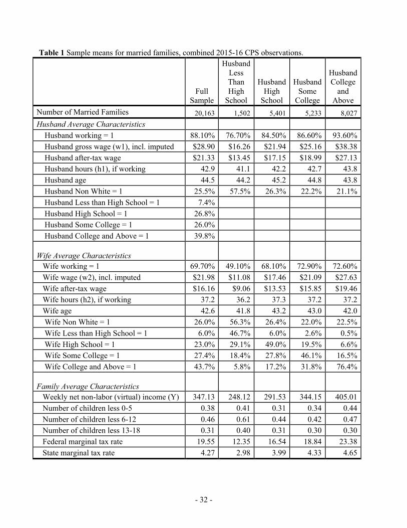
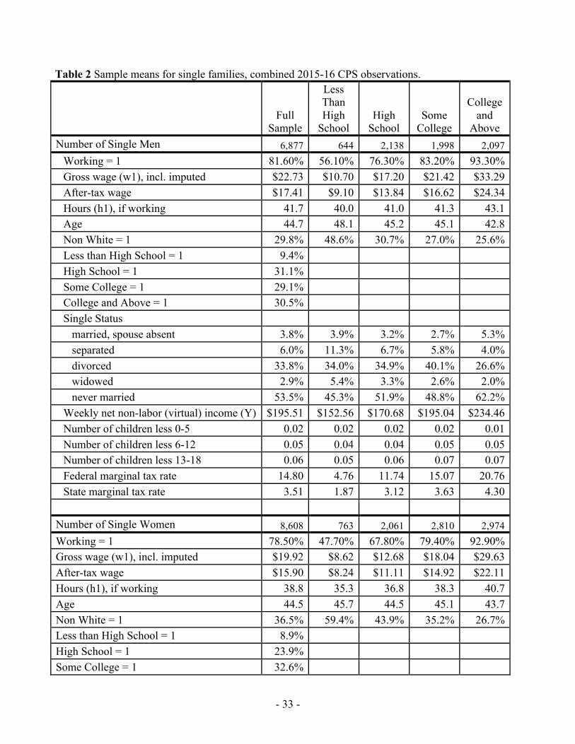
Tables 1 and 2 contain the means for the full sample and for each sub-sample based on

education, for married and single families (respectively). We have a total of 20,163 married

families and 15,485 single families in our sample. Among married families, about 88 percent of

husbands and nearly 70 percent of wives are working (with both percentages increasing in

husband's education). Husbands work more hours (43) and earn a higher after-tax hourly wage

($21.33 after tax) than their wives, who work about 37 hours and earn $16.16 after tax. Husbands

are slightly older than wives, at 45 vs. 43 years of age. Wives are slightly more educated than

their husbands. The families have roughly $347 per week in (virtual) non-labor income. Virtual

non-labor income is what the non-labor income for the family would be if the portion of the non-

linear constraint they are on were extended to the vertical axis. The average federal (state)

13 http:// www.nber.org/~ taxsim/; see also Feenberg and Coutts (1993). In addition to the detained income source information from the CPS data, we also include information on property tax, CPS imputed capital gains and capital losses. All households are classified as if they were declaring taxes jointly and the main earner is identified as that with the highest total earned income. The tax simulation was implemented using the Stata taxsim interface. Data was prepared based on the recommendations found at http://users.nber.org/~taxsim/to-taxsim/cps/.

- 16 -

marginal tax rate across families is 20 percent (4 percent).

[Tables 1 and 2 about here]

Women comprise 56 percent of the single persons sample. On average, women have

slightly more education; are slightly younger than the men; work fewer hours (39 vs. 42 for

single men); have about the same non-labor (virtual) income; have a greater number of children;

and earn lower wages. The majority of singles have never been married (46 percent of women

and 54 percent of men), followed by singles who are divorced.

4 Results

4.1 Utility Function Parameter Estimates and Labor Supply Elasticities

Maximum likelihood estimates of the utility function parameters for both married and

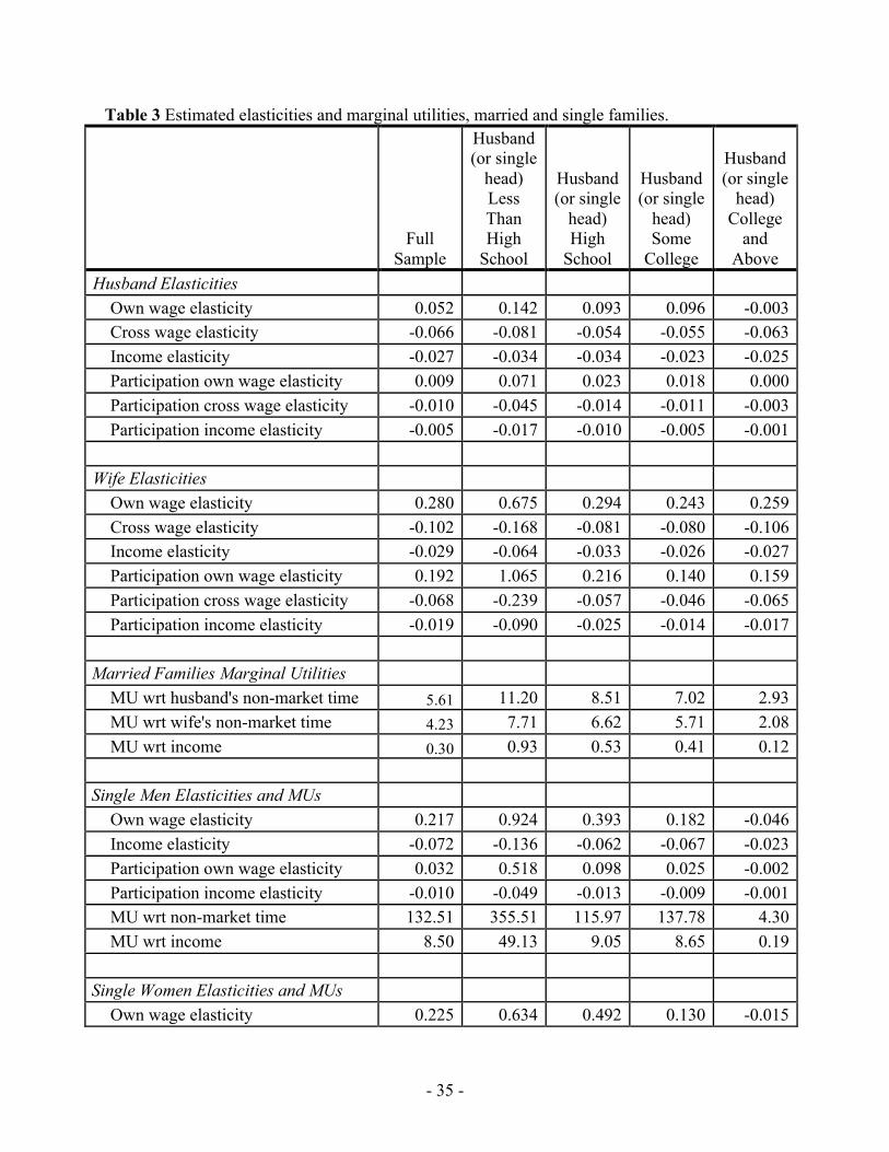
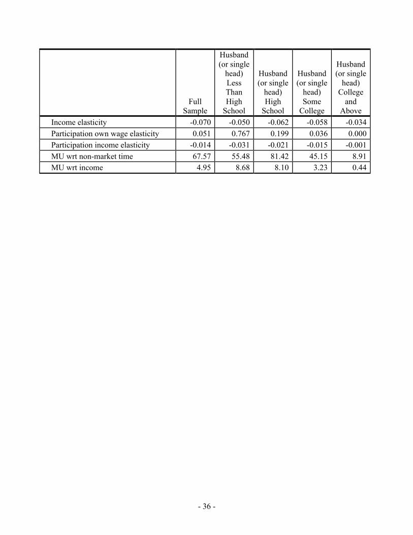
single families are presented in Appendix D. Average elasticity estimates for married and single

families, along with estimates of marginal utilities, are found in Table 3. For purposes of placing

the estimated elasticities in context of the literature, Figure 1 illustrates the intensive margin

elasticities along with others' estimates of these elasticities. Note that own wage elasticities are

averaged across workers and non-workers. The bottom line is that our elasticity estimates

generally fall within the range of those found in the literature.

[Table 3 and Figure 1 about here]

Note that married women's own wage elasticities are higher than married men's

elasticities, indicating that women's labor supply is more responsive to changes in their own

wages. In addition, married women are more responsive to changes in their own wages than are

single women, who average an own-wage elasticity very close to that of single men. The

estimated negative cross-wage elasticities (among married families) indicate that husbands and

wives view their non-market time as substitutes. Cross wage elasticities for husbands and wives

- 17 -

correspond to families in which both members are working. Both men and women present the

expected negative income elasticity. The bottom line from these estimates of labor supply

elasticities is that the simulation will be based on behavior reflected through labor supply

elasticities consistent with those estimated by others, using different data, empirical models, and

for different purposes, suggesting that our estimates are in line with other's estimates. Appendix

E provides a sensitivity analysis showing that our results are robust to variations in labor supply

elasticities. The results from this sensitivity analysis are discussed below.

4.2 Expected Welfare Loss From a Shock to Unemployment

By dividing the calculated expected loss in welfare from a one-percentage point rise in

the unemployment rate (in utils) by the family's marginal utility of income/consumption (𝑈!), we

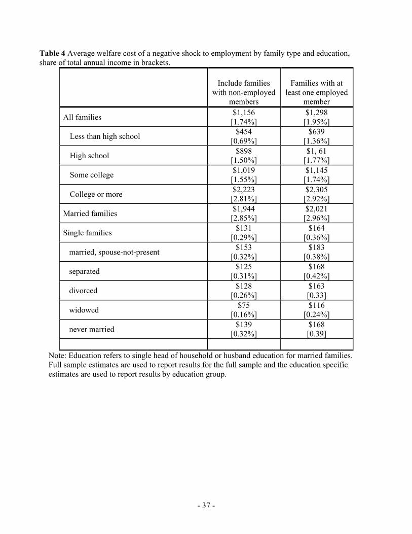
get a dollar value of that expected welfare loss. Table 4 reports the annualized dollar value for

the expected welfare loss from a positive shock to unemployment for families of different types

and education levels (the loss as a share of total household income is also reported).14

[Table 4 about here]

Workers at higher education levels earn higher wages, putting upward pressure on the

expected welfare loss from non-employment. For example, the average annual income for

families with at least a college degree is more than four times larger than families with less than

a high school degree (i.e., roughly $88,000 vs. $34,000). Therefore, families with higher

education (higher earnings) have much more to lose if they are hit by non-employment.

However, a higher education level also means a lower probability of being hit by non-

employment, putting downward pressure on the expected welfare loss from rising

14 This is not to imply that an analogous negative shock to the unemployment rate would generate a symmetric gain in welfare for families. In fact, De Neve et al. (2017) find that subjective well-being is more sensitive to negative economic conditions than to positive economic conditions.

- 18 -

unemployment. For example, a one percentage point rise in the unemployment increases the

probability of non-employment for someone with less than a college degree by 1.23 percentage

points, whereas the marginal effect on someone with a college degree is only 0.54 percent points.

Based on the results in Table 4, we see that, since the expected welfare loss increases with

education, the impact of the potential of losing higher wages dominates the lower probability of

non-employment.

The average annualized expected welfare loss for the whole sample is $1,156. To put this

figure into perspective, consider that a recent survey finds that 63 percent of Americans report

that they do not have enough savings to face an unexpected expense of $500 to $1,000 (Picchi

2016; also see Trubey 2016). So, a loss of $1,156 would be significant for a majority of

American families. This estimate of expected welfare loss is much lower than that found in Hurd

(1980), who estimates an individual welfare loss per unemployment spell of about $7,000 (in

2012 dollars). One reason Hurd's estimate is so much higher than ours is that we are estimating

the expected welfare loss from non-employment, rather than the actual cost of a specific job loss.

In addition, his model does not allow for any positive utility gained from additional non-market

time that results from unemployment, nor the potential mitigating effects of unemployment

insurance.

There is a significant difference between single and married families -- the average

expected welfare loss overall is $1,944 among married families, whereas the average annualized

expected loss is only $131 among singles. To explain this difference one might first look at the

relative valuation that singles and married individuals place on non-market time and income (the

marginal utilities in Table 3). If a household values non-market time more, relative to income,

the expected loss from unemployment would be lower. However, from those tables we can see

- 19 -

that, overall, married and single families have similar non-market time/income marginal utility

ratios. The ratio is 15.6 and 13.7 for single women and men, respectively, and among married

households it is 18.7 for husbands' non-market time and 14.1 for wives' non-market time.

Another possibility is that with two people in the household, the chance of taking a "hit"

from unemployment essentially doubles for married families. The only households that will be

completely unaffected by a rise in the unemployment rate are those with no workers in the

household. Among singles, this is about 20 percent of families, whereas the percent of married

families with no workers is only four percent. However, this explanation is lacking, as well,

since if we exclude singles who are not working from the calculation, the average annual

expected loss from unemployment increases to only $164. This lower cost of unemployment

varies a bit across family status among singles, as well. The average annualized loss ranges from

$76 for widows, $139 for never married, $125 for separated, $128 for divorced, to $154 for

households with the spouse-not-present.

The primary significant difference between married and single families affecting their

average expected welfare loss from a rise in the unemployment rate appears to be the difference

in their total income levels. On average, married families have more than twice the level of total

income than single families (i.e., roughly $84,000 vs. $40,000). In addition, the probability of at

least one person in a household being non-employed when the unemployment rate rises by one

percentage point increases by more in a married household than in a single household -- by 1.8

percentage points for a married household and by 0.95 percentage points in a single household,

on average.15

15 The amount by which the probability of non-employment for at least one member of a married household increases is calculated by one minus the increased probability of both members being hit by non-employment. Specifically, the average marginal effect of a one percentage point

- 20 -

Note that concluding that the welfare loss from a one percentage point rise in the

unemployment rate is greater for married families than for single families, and is greater for the

more educated, does not say anything about the welfare levels of different family types or

education levels. In addition, welfare costs of a rise in the unemployment rate discussed here do

not take into account the potential long term consequences of job loss on the mental and physical

health of those impacted and/or their children or on lifetime wealth. For example, see

Golberstein, Gonzales, and Meara (2016); Sullivan and Wachter (2009); Mathers and Schofield

(1998); Krueger, Mitman, and Perri (2016). Nor does our estimate of the expected welfare cost

of rising unemployment take into account any fear that families or individuals might have of

losing their job (as DiTella, MacCulloch, and Oswald 2001 claim their survey of happiness

does).

4.3 Equivalent Welfare loss from an Unanticipated Price Level Change

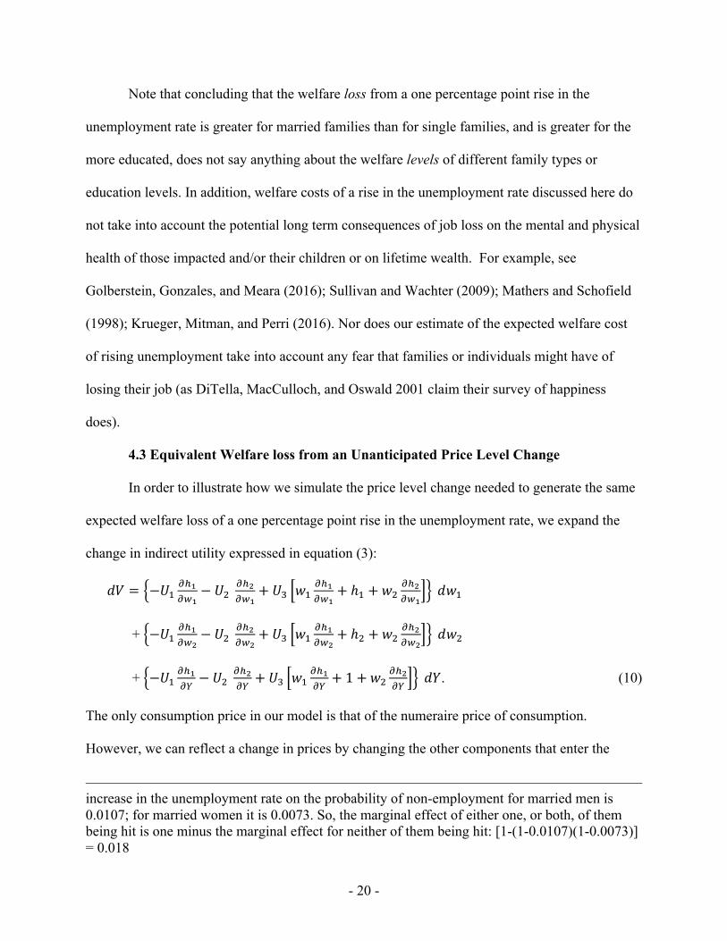
In order to illustrate how we simulate the price level change needed to generate the same

expected welfare loss of a one percentage point rise in the unemployment rate, we expand the

change in indirect utility expressed in equation (3):

𝑑𝑉 = −𝑈!!!!!!!

− 𝑈!  !!!!!!

+ 𝑈! 𝑤!!!!!!!

+ ℎ! + 𝑤!!!!!!!

 𝑑𝑤!

+   −𝑈!!!!!!!

− 𝑈!  !!!!!!

+ 𝑈! 𝑤!!!!!!!

+ ℎ! + 𝑤!!!!!!!

 𝑑𝑤!

+   −𝑈!!!!!!− 𝑈!  

!!!!!+ 𝑈! 𝑤!

!!!!!+ 1+ 𝑤!

!!!!!

 𝑑𝑌. (10)

The only consumption price in our model is that of the numeraire price of consumption.

However, we can reflect a change in prices by changing the other components that enter the

increase in the unemployment rate on the probability of non-employment for married men is 0.0107; for married women it is 0.0073. So, the marginal effect of either one, or both, of them being hit is one minus the marginal effect for neither of them being hit: [1-(1-0.0107)(1-0.0073)] = 0.018

- 21 -

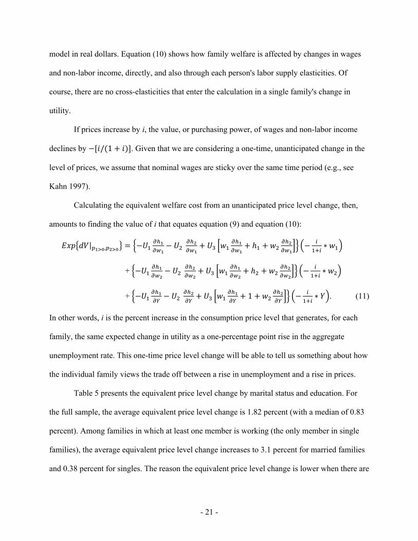
model in real dollars. Equation (10) shows how family welfare is affected by changes in wages

and non-labor income, directly, and also through each person's labor supply elasticities. Of

course, there are no cross-elasticities that enter the calculation in a single family's change in

utility.

If prices increase by i, the value, or purchasing power, of wages and non-labor income

declines by −[𝑖/(1+ 𝑖)]. Given that we are considering a one-time, unanticipated change in the

level of prices, we assume that nominal wages are sticky over the same time period (e.g., see

Kahn 1997).

Calculating the equivalent welfare cost from an unanticipated price level change, then,

amounts to finding the value of i that equates equation (9) and equation (10):

𝐸𝑥𝑝 𝑑𝑉 !!!!,!!!! = −𝑈!!!!!!!

− 𝑈!  !!!!!!

+ 𝑈! 𝑤!!!!!!!

+ ℎ! + 𝑤!!!!!!!

− !!!!

∗ 𝑤!

+   −𝑈!!!!!!!

− 𝑈!  !!!!!!

+ 𝑈! 𝑤!!!!!!!

+ ℎ! + 𝑤!!!!!!!

− !!!!

∗ 𝑤!

+   −𝑈!!!!!!− 𝑈!  

!!!!!+ 𝑈! 𝑤!

!!!!!+ 1+ 𝑤!

!!!!!

− !!!!

∗ 𝑌 . (11)

In other words, i is the percent increase in the consumption price level that generates, for each

family, the same expected change in utility as a one-percentage point rise in the aggregate

unemployment rate. This one-time price level change will be able to tell us something about how

the individual family views the trade off between a rise in unemployment and a rise in prices.

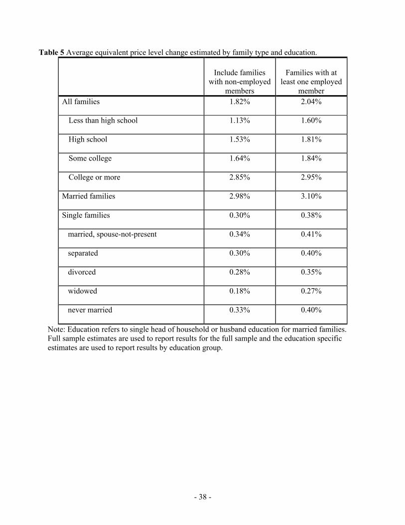
Table 5 presents the equivalent price level change by marital status and education. For

the full sample, the average equivalent price level change is 1.82 percent (with a median of 0.83

percent). Among families in which at least one member is working (the only member in single

families), the average equivalent price level change increases to 3.1 percent for married families

and 0.38 percent for singles. The reason the equivalent price level change is lower when there are

- 22 -

non-employed members in the household is because any rise in the unemployment rate has no

impact on individuals who are already out of the labor force, so the expected loss from

unemployment is less.

[Table 5 about here]

The unanticipated equivalent price level change is much lower among single families at

0.30 percent (0.21 percent at the median). Since the cost of a one-percentage point rise in the

unemployment rate is not as costly to them, singles, if given a choice, would not willingly endure

as large a shock to prices in order to avoid a rise in unemployment. If we interpret this valuation

of an unanticipated shock to prices as reflective of a short-term reaction to unanticipated

inflation, this result is consistent with Burdett et al. (2016) who find that singles are much more

likely to hold cash than non-singles, which loses value more quickly with inflation than other

assets; they conclude that, "...inflation is a tax on being single" (p. 352).16 While we get there

from a very different empirical strategy, our results point to the same conclusion. In addition,

Burdett et al. find that among the non-married, inflation is likely to be most costly to those who

are widowed; we find the same, as illustrated in Table 5.

Another point of comparison for these results is the work by DiTella, MacCulloch, and

Oswald (2001). Their analysis across countries and time finds that, "a 1-percentage-point

increase in the unemployment rate equals the loss brought about by an extra 1.66 percentage

points of inflation" (p. 339). Again, their analysis is quite different from the one presented here --

they estimate life satisfaction as a function of unemployment and inflation across many countries

and time. And, although they do not provide the nuances seen here across demographics, their

16 Also see Aruoba, Davis, and Wright (2016). Other research (Alm, Whittington, and Fletcher 2002) has identified a tax on singles (relative to others with similar economic and demographic characteristics) through the structure of the U.S. tax system, however it is unclear how inflation would make that worse.

- 23 -

estimated inflation generated loss of happiness (or, welfare) equivalent to 1pp rise in the

unemployment rate is within the range of the equivalent price level changes presented in Table 5.

As mentioned earlier, Appendix E contains the results from a sensitivity analysis for the

equivalent price level changes presented in Table 5. For the full sample of married families, the

alternate price level changes, using alternative elasticities found in the literature, range from a

low of 2.69 to a high of 3.95 percent (around our estimate of 2.98 percent). For single men and

women, there is no measurable difference in the estimates using alternative labor supply

elasticities. The estimates presented here for the expected welfare cost of unemployment and its

equivalent shock to prices are clearly not being driven by differences found between our labor

supply elasticities and those in the rest of the literature.

4.4 Unanticipated Price Level Change vs. Unemployment Shock Trade-off

There is a rich literature that estimates the cost of inflation in terms of how much

consumption one would be willing to give up to lower inflation, typically from 10 percent to

some target level (see Lagos, Rocheteau, and Wright, Forthcoming). The estimates of the

inflation/consumption trade-off range between 2 (Lagos and Wright 2005) and 1.25 (Dong

2010). An estimate greater than one implies a greater value placed on lowering inflation than the

resulting loss in consumption.17

We can make a similar trade-off assessment by comparing the equivalent welfare cost of

an unanticipated rise in prices and the expected welfare cost of a shock to unemployment as a

percent of total income. This requires assuming that the welfare cost of an unanticipated rise in

prices is reflective of the short-term welfare impact of an unanticipated increase in inflation.

17 A trade-off value greater than one is also consistent with Low, Meghir, and Pistaferri (2010), who find, in a life-cycle model, that individuals value the risk of wage loss (productivity) more than the risk of employment loss (job destruction).

- 24 -

Figure 2 plots these losses along with the ratio of the two reflecting their trade-off.18 A ratio

greater than one implies a greater loss from an unanticipated rise in prices than an equivalent

welfare shock from a one percentage-point rise in the unemployment rate.

[Figure 2 about here]

Panel (a) of Figure 2 illustrates, for all families combined, that the cost of a one

percentage-point equivalent rise in prices increases with income in the lower half of the income

distribution, then basically flattens out. The expected loss from an increase in unemployment, as

a percent of income (panel b), also rises in the lower half of the income distribution, but then

declines as income continues to rise. This declining welfare loss from unemployment is more

dramatic among married families (see Appendix F) and is consistent with Krueger, Mitman, and

Perri (2016) who find that the loss to lifetime consumption from higher unemployment during

recessions represents a lower share of income in wealthier households.

Panel (c) shows the ratio of the welfare loss from a price level change relative to the

welfare loss from a shock to unemployment. This ratio is less than one for the bottom half of the

distribution, indicating that for lower-income families, the welfare loss from rising prices is less

than the expected welfare loss from a rise in unemployment (as a share of total income). In the

upper half of the income distribution, the welfare loss from a shock to prices exceeds the

expected welfare loss from a shock to unemployment. This comparison is made separately for

married and single families in Appendix F. In spite of the dramatically different annualized

dollar amount of expected loss from a one percentage point rise in the unemployment rate, and

hence tolerance for unanticipated price level changes, the price shock/unemployment shock

welfare loss trade-off produces similar results across family types. As a percent of total income,

18 Differences between married and single families can be seen in Appendix F.

- 25 -

a shock to unemployment is worse than an equivalent price level change for those below the

median income level and vice verse for those above the median.

5 Conclusions and Implications

Awareness of the personal or family welfare cost of a shock to unemployment and how

that cost varies across families is of interest due to the distributional implications of policy that

might affect the labor market. We find, on average, that the expected loss to family welfare of a

one-percentage point rise in the aggregate unemployment rate is equivalent to an annualized

dollar amount of $1,156. We also find a considerable amount of heterogeneity across families,

which means that aggregate averages yield very different answers than looking more closely at

population sub-groups. For example, the expected welfare cost of a shock to unemployment is

much higher among married (vs. single) families and increases for both in education/income

levels.

We also find that an unanticipated increase in prices of about 1.8%, on average for all

families, produces a welfare loss equivalent to that generated by a one percentage point shock to

unemployment and is much lower for single families than for married families. If reflective of a

short-term reaction to inflation, then this result is consistent with Burdett et al.'s (2016) finding

that inflation places a larger tax on singles. On average singles would only be willing to trade an

increase in prices of roughly one-third of a percent to avoid a one percentage point rise in the

unemployment rate, whereas married families would tolerate a price level increase of up to three

percent to avoid the same degree of unemployment rate shock.

Additionally, we find that the welfare loss from a rise in prices vs. a shock to

unemployment as a share of total income increases with income, suggesting that those in the

lower end of the income distribution experience a greater welfare loss as a percent of total

- 26 -

income from a shock to unemployment relative to an unanticipated price level increase, but vice

versa for those in the upper end of the income distribution. This conclusion holds for both

married and single families, suggesting that, regardless of family structure and overall dollar

equivalent value of the expected loss from a rise in the unemployment rate, the welfare trade-off

between unemployment and an unanticipated rise in prices varies consistently across the income

distribution.

- 27 -

References

Aaronson, Daniel, and Eric French. 2009. “The Effects of Progressive Taxation on Labor Supply When Hours and Wages Are Jointly Determined.” The Journal of Human Resources 44 (2): 386–408. http://www.jstor.org/stable/20648902.

Alm, James, Leslie A. Whittington, and Jason Fletcher. 2002. “Is There a ‘Singles Tax’? The Relative Income Tax Treatment of Single Households.” Public Budgeting & Finance 22 (2): 69–86. doi:10.1111/1540-5850.00074.

Amaral, Pedro. 2017. “Monetary Policy and Inequality.” Clevelandfed. January 10. https://www.clevelandfed.org:443/newsroom and events/publications/economic commentary/2017 economic commentaries/ec 201701 monetary policy and inequality.

Amemiya, Takeshi. 1974. “Multivariate Regression and Simultaneous Equation Models When the Dependent Variables Are Truncated Normal.” Econometrica 42 (6): 999–1012. doi:10.2307/1914214.

Anderson, Patricia M., and Bruce D. Meyer. 1997. “Unemployment Insurance Takeup Rates and the After-Tax Value of Benefits.” The Quarterly Journal of Economics 112 (3): 913–37. http://www.jstor.org/stable/2951259.

Apps, Patricia, and Ray Rees. 2009. Public Economics and the Household. Cambridge, UK: Cambridge University Press.

Aruoba, S. Borağan, Morris A. Davis, and Randall Wright. 2016. “Homework in Monetary Economics: Inflation, Home Production, and the Production of Homes.” Review of Economic Dynamics 21 (July): 105–24. doi:10.1016/j.red.2014.09.009.

Bahl, Roy, Richard Hawkins, Robert E. Moore, and David L. Sjoquist. 1993. “Using Microsimulation Models for Revenue Forecasting in Developing Countries.” Public Budgeting and Financial Management 5 (1): 159–86.

Berentsen, Aleksander, Guido Menzio, and Randall Wright. 2011. “Inflation and Unemployment in the Long Run.” American Economic Review 101 (1): 371–98. doi:10.1257/aer.101.1.371.

Bernanke, Ben S. 2015. “Monetary Policy and Inequality.” Brookings. June 1. https://www.brookings.edu/blog/ben-bernanke/2015/06/01/monetary-policy-and-inequality/.

Bishop, Kelly, Bradley Heim, and Kata Mihaly. 2009. “Single Women’s Labor Supply Elasticities: Trends and Policy Implications.” Industrial and Labor Relations Review 63 (1): 146–68. http://www.jstor.org/stable/25594548.

Blank, Rebecca M., and David E. Card. 1991. “Recent Trends in Insured and Uninsured Unemployment: Is There an Explanation?” The Quarterly Journal of Economics 106 (4): 1157–89. doi:10.2307/2937960.

Blau, Francine D., and Lawrence M. Kahn. 2007. “Changes in the Labor Supply Behavior of Married Women: 1980–2000.” Journal of Labor Economics 25 (3): 393–438. doi:10.1086/513416.

Blundell, Richard. 1992. “Labour Supply and Taxation: A Survey.” Fiscal Studies 13 (3): 15–40. doi:10.1111/j.1475-5890.1992.tb00181.x.

Blundell, Richard, Pierre-Andre Chiappori, Thierry Magnac, and Costas Meghir. 2007. “Collective Labour Supply: Heterogeneity and Non-Participation.” The Review of Economic Studies 74 (2): 417–45.

- 28 -

Blundell, Richard, Alan Duncan, Julian McCRAE, and Costas Meghir. 2000. “The Labour Market Impact of the Working Families’ Tax Credit.” Fiscal Studies 21 (1): 75–104. doi:10.1111/j.1475-5890.2000.tb00581.x.

Blundell, Richard, and Thomas Macurdy. 1999. “Labor Supply: A Review of Alternative Approaches.” In Handbook of Labor Economics, Orley Ashenfelter and David Card, 3A:1559–1695. Amsterdam: Elsevier. https://ideas.repec.org/h/eee/labchp/3-27.html.

Blundell, Richard, Costas Meghir, Elizabeth Symons, and Ian Walker. 1988. “Labour Supply Specification and the Evaluation of Tax Reforms.” Journal of Public Economics 36 (1): 23–52. doi:10.1016/0047-2727(88)90021-7.

Burdett, Kenneth, Mei Dong, Ling Sun, and Randall Wright. 2016. “Marriage, Markets, and Money: A Coasian Theory of Household Formation.” International Economic Review 57 (2): 337–68. doi:10.1111/iere.12160.

Chetty, Raj. 2008. “Moral Hazard versus Liquidity and Optimal Unemployment Insurance.” Journal of Political Economy 116 (2): 173–234.

———. 2012. “Bounds on Elasticities With Optimization Frictions: A Synthesis of Micro and Macro Evidence on Labor Supply.” Econometrica 80 (3): 969–1018. doi:10.3982/ECTA9043.

Cullen, Julie Berry, and Jonathan Gruber. 2000. “Does Unemployment Insurance Crowd out Spousal Labor Supply?” Journal of Labor Economics 18 (3): 546–72. doi:10.1086/209969.

Currie, Janet. 2006. “The Take-up of Social Benefits.” In Poverty, the Distribution of Income, and Public Policy, A. Auerbach, D. Card, J. Quigley (Eds.), 80–148. New York: Russell Sage.

De Neve, Jan-Emmanuel, George Ward, Femke De Keulenaer, Bert Van Landeghem, Georgios Kavetsos, and Michael I. Norton. 2017. “The Asymmetric Experience of Positive and Negative Economic Growth: Global Evidence Using Subjective Well-Being Data.” The Review of Economics and Statistics, August. doi:10.1162/REST_a_00697.

Devereux, Paul J. 2004. “Changes in Relative Wages and Family Labor Supply.” The Journal of Human Resources 39 (3): 696–722. doi:10.2307/3558993.

DiTella, Rafael, Robert J. MacCulloch, and Andrew J. Oswald. 2001. “Preferences over Inflation and Unemployment: Evidence from Surveys of Happiness.” The American Economic Review 91 (1): 335–41. http://www.jstor.org/stable/2677914.

Dong, Mei. 2010. “Inflation and Variety*.” International Economic Review 51 (2): 401–20. doi:10.1111/j.1468-2354.2010.00585.x.

Dong, Mei, Ling Sun, and Randall Wright. 2015. “Macroeconomic Policy and Household Economics.” Working Paper. Economic Policy Papers. Minneapolis, MN: Federal Reserve Bank of Minneapolis. https://www.minneapolisfed.org/research/economic-policy-papers/macroeconomic-policy-and-household-economics.

Ebenstein, Avraham, and Kevin Stange. 2010. “Does Inconvenience Explain Low Take-up? Evidence from Unemployment Insurance.” Journal of Policy Analysis and Management 29 (1): 111–36. doi:10.1002/pam.20481.

Edwards, Kathryn Anne. 2015. “Who Helps the Unemployed? Young Workers’ Receipt of Private Cash Transfers.” SSRN Scholarly Paper ID 2698344. Rochester, NY: Social Science Research Network. http://papers.ssrn.com/abstract=2698344.

Eissa, Nada, Henrik Jacobsen Kleven, and Claus Thustrup Kreiner. 2008. “Evaluation of Four Tax Reforms in the United States: Labor Supply and Welfare Effects for Single

- 29 -

Mothers.” Journal of Public Economics 92 (3–4): 795–816. doi:10.1016/j.jpubeco.2007.08.005.

Federal Reserve Bank of Philadelphia. 2017. “Fourth Quarter 2016 Survey of Professional Forecasters - Philadelphia Fed.” Accessed February 14. https://www.philadelphiafed.org/research-and-data/real-time-center/survey-of-professional-forecasters/2016/survq416.

Feenberg, Daniel, and Elisabeth Coutts. 1993. “An Introduction to the TAXSIM Model.” Journal of Policy Analysis and Management 12 (1): 189–94. doi:10.2307/3325474.

Fiorio, Carlo V. 2008. “Analysing Tax—Benefit Reforms Using Non-Parametric Methods.” Fiscal Studies 29 (4): 499–522. http://www.jstor.org/stable/24440099.

Fuller, David L., B. Ravikumar, and Yuzhe Zhang. 2012. “Unemployment Insurance: Payments, Overpayments and Unclaimed Benefits.” The Regional Economist. October. https://www.stlouisfed.org/~/media/Files/PDFs/publications/pub_assets/pdf/re/2012/d/Unemployment.pdf.

Golberstein, Ezra, Gilbert Gonzales, and Ellen Meara. 2016. “Economic Conditions and Children’s Mental Health.” Working Paper 22459. National Bureau of Economic Research. http://www.nber.org/papers/w22459.

Gordon, Robert J., William Nordhaus, and William Poole. 1973. “The Welfare Cost of Higher Unemployment.” Brookings Papers on Economic Activity 1973 (1): 133–205. doi:10.2307/2534086.

Gramlich, Edward M. 1974. “The Distributional Effects of Higher Unemployment.” Brookings Papers on Economic Activity 1974 (2): 293–336. doi:10.2307/2534189.

Hall, Robert E. 1973. “Wages, Income, and Hours of Work in the U.S. Labor Force.” In Income Maintenance and Labor Supply, edited by Glen G. Cain and Harold W. Watts, 102–62. Chicago, IL: University of Chicago Press.

———. 1981. “Comment on S. fischer ‘Relative Shocks, Relative Price Variability, and Inflation.’” Brookings Papers on Economic Activity 2: 432–34.

Heckman, James. 1974. “Shadow Prices, Market Wages, and Labor Supply.” Econometrica 42 (4): 679–94. doi:10.2307/1913937.

Heim, Bradley T. 2009. “Structural Estimation of Family Labor Supply with Taxes: Estimating a Continuous Hours Model Using a Direct Utility Specification.” Journal of Human Resources 44 (2): 350–85. doi:10.1353/jhr.2009.0002.

Herrnstein, Richard J., and Charles A. Murray. 1994. The Bell Curve: Intelligence and Class Structure in American Life. New York: Free Press.

Hotchkiss, Julie L., Mary Mathewes Kassis, and Robert E. Moore. 1997. “Running Hard and Falling behind: A Welfare Analysis of Two-Earner Families.” Journal of Population Economics 10 (3): 237–50. http://www.jstor.org/stable/20007544.

Hotchkiss, Julie L., Robert E. Moore, and Fernando Rios-Avila. 2012. “Assessing the Welfare Impact of Tax Reform: A Case Study of the 2001 U.S. Tax Cut.” Review of Income and Wealth 58 (2): 233–56. doi:10.1111/j.1475-4991.2012.00493.x.

Hotchkiss, Julie L., Robert E. Moore, Fernando Rios-Avila, and Melissa R. Trussell. 2017. “A Tale of Two Decades: Relative Intra-Family Earning Capacity and Changes in Family Welfare over Time.” Review of Economics of the Household 15 (3): 707–37. https://ideas.repec.org/a/kap/reveho/v15y2017i3d10.1007_s11150-016-9354-9.html.

- 30 -

Hurd, Michael. 1980. “A Compensation Measure of the Cost of Unemployment to the Unemployed.” The Quarterly Journal of Economics 95 (2): 225–43. doi:10.2307/1885497.

Imai, Susumu, and Michael P. Keane. May2004. “Intertemporal Labor Supply and Human Capital Accumulation.” International Economic Review 45 (2): 601–41. http://www.jstor.org/stable/3663533.

Kahn, Shulamit. 1997. “Evidence of Nominal Wage Stickiness from Microdata.” The American Economic Review 87 (5): 993–1008. http://www.jstor.org/stable/2951337.

Keane, Michael P. 2011. “Labor Supply and Taxes: A Survey.” Journal of Economic Literature 49 (4): 961–1075. doi:10.1257/jel.49.4.961.

Kettemann, Adreas. 2014. “Unemployment Insurance Takeup and the Business Cycle.” Working Paper. Zurich, Germany: University of Zurich. http://www.iza.org/conference_files/wagerigidities_2014/kettemann_a10097.pdf.

Krueger, Dirk, Kurt Mitman, and Fabrizio Perri. 2016. “On the Distribution of the Welfare Losses of Large Recessions.” Working Paper 22458. National Bureau of Economic Research. http://www.nber.org/papers/w22458.

Krusell, Per, and Anthony A Smith. 1999. “On the Welfare Effects of Eliminating Business Cycles.” Review of Economic Dynamics 2 (1): 245–72. doi:10.1006/redy.1998.0043.

Kumar, Anil. 2009. “Nonparametric Estimation of the Impact of Taxes on Female Labor Supply.” Journal of Applied Econometrics 27 (3): 415–39. doi:10.1002/jae.1205.

Lagos, Ricardo, Guillaume Rocheteau, and Randall Wright. Forthcoming. “Liquidity: A New Monetarist Perspective.” Journal of Economic Literature. http://econweb.ucsd.edu/~rstarr/281webpage/Lagos_Rochetau_Wright.pdf.

Lagos, Ricardo, and Randall Wright. 2005. “A Unified Framework for Monetary Theory and Policy Analysis.” Journal of Political Economy 113 (3): 463–84. doi:10.1086/429804.

Lam, David. 1988. “Marriage Markets and Assortative Mating with Household Public Goods: Theoretical Results and Empirical Implications.” The Journal of Human Resources 23 (4): 462–87. doi:10.2307/145809.

Low, Hamish, Costas Meghir, and Luigi Pistaferri. 2010. “Wage Risk and Employment Risk over the Life Cycle.” American Economic Review 100 (4): 1432–67. doi:10.1257/aer.100.4.1432.

Lucas, Robert E. 1991. Models of Business Cycles. Oxford, OX, UK; Cambridge, Mass., USA: Wiley-Blackwell.

Mathers, C.D., and D.J. Schofield. 1998. “The Health Consequences of Unemployment: The Evidence.” The Medical Journal of Australia 168 (4): 178–82. http://europepmc.org/abstract/med/9507716.

McClelland, Robert, and Shannon Mok. 2012. “A Review of Recent Research on Labor Supply Elasticities.” Working Paper 2012–12. Washington, D.C.: Congressional Budget Office.

McElroy, Marjorie B. 1990. “The Empirical Content of Nash-Bargained Household Behavior.” The Journal of Human Resources 25 (4): 559–83. doi:10.2307/145667.

Michaelides, Marios, and Peter R. Mueser. 2012. “Recent Trends in the Characteristics of Unemployment Insurance Recipients.” Monthly Labor Review 135 (7): 28–47.

Moreau, Nicolas, and Olivier Bargain. 2005. “Is the Collective Model of Labor Supply Useful for Tax Policy Analysis? A Simulation Exercise.” SSRN Scholarly Paper ID 396040. Rochester, NY: Social Science Research Network. http://papers.ssrn.com/abstract=396040.

- 31 -

Muthen, Bengt. 1990. “Moments of the Censored and Truncated Bivariate Normal Distribution.” British Journal of Mathematical and Statistical Psychology 43 (1): 131–43. doi:10.1111/j.2044-8317.1990.tb00930.x.

Nakajima, Makoto. 2015. “Te Redistributive Consequences of Monetary Policy.” Business Review. Federal Reserve Bank of Philadelphia. file:///Users/f1jlh01/Desktop/brQ215_the_redistributive_consequences_of_monetary_policy.pdf.

Okun, Arthur M. 1962. “Potential GNP: Its Measurement and Significance.” Proceedings of the Business and Economics Statistics Section of the Am Statistical Assoc, 98–104.

Pencavel, John. 2002. “A Cohort Analysis of the Association between Work Hours and Wages among Men.” The Journal of Human Resources 37 (2): 251–74. doi:10.2307/3069647.

Picchi, Aimee. 2016. “Most Americans Can’t Handle a $500 Surprise Bill - CBS News.” News. CPS Moneywatch. January 6. http://www.cbsnews.com/news/most-americans-cant-handle-a-500-surprise-bill/.

Ransom, Michael R. 1987. “An Empirical Model of Discrete and Continuous Choice in Family Labor Supply.” The Review of Economics and Statistics 69 (3): 465–72. doi:10.2307/1925534.

Sullivan, Daniel, and Till von Wachter. 2009. “Job Displacement and Mortality: An Analysis Using Administrative Data.” The Quarterly Journal of Economics 124 (3): 1265–1306. doi:10.1162/qjec.2009.124.3.1265.

Triest, Robert K. 1990. “The Effect of Income Taxation on Labor Supply in the United States.” The Journal of Human Resources 25 (3): 491–516. doi:10.2307/145991.

Trubey, Scott. 2016. “How Would You Pay for an Unexpected $400 Expense?” Ajc.com. Accessed November 1. http://www.ajc.com/business/could-you-pay-for-unexpected-400-expense/3GZRJGMrlisK21Z0rxpI6N/.

- 32 -

Table 1 Sample means for married families, combined 2015-16 CPS observations.

Full Sample

Husband Less Than High

School

Husband High

School

Husband Some

College

Husband College

and Above

Number of Married Families 20,163 1,502 5,401 5,233 8,027 Husband Average Characteristics

Husband working = 1 88.10% 76.70% 84.50% 86.60% 93.60% Husband gross wage (w1), incl. imputed $28.90 $16.26 $21.94 $25.16 $38.38 Husband after-tax wage $21.33 $13.45 $17.15 $18.99 $27.13 Husband hours (h1), if working 42.9 41.1 42.2 42.7 43.8 Husband age 44.5 44.2 45.2 44.8 43.8 Husband Non White = 1 25.5% 57.5% 26.3% 22.2% 21.1% Husband Less than High School = 1 7.4% Husband High School = 1 26.8% Husband Some College = 1 26.0% Husband College and Above = 1 39.8%

Wife Average Characteristics Wife working = 1 69.70% 49.10% 68.10% 72.90% 72.60% Wife wage (w2), incl. imputed $21.98 $11.08 $17.46 $21.09 $27.63 Wife after-tax wage $16.16 $9.06 $13.53 $15.85 $19.46 Wife hours (h2), if working 37.2 36.2 37.3 37.2 37.2 Wife age 42.6 41.8 43.2 43.0 42.0

Wife Non White = 1 26.0% 56.3% 26.4% 22.0% 22.5% Wife Less than High School = 1 6.0% 46.7% 6.0% 2.6% 0.5% Wife High School = 1 23.0% 29.1% 49.0% 19.5% 6.6% Wife Some College = 1 27.4% 18.4% 27.8% 46.1% 16.5% Wife College and Above = 1 43.7% 5.8% 17.2% 31.8% 76.4%

Family Average Characteristics Weekly net non-labor (virtual) income (Y) 347.13 248.12 291.53 344.15 405.01 Number of children less 0-5 0.38 0.41 0.31 0.34 0.44 Number of children less 6-12 0.46 0.61 0.44 0.42 0.47 Number of children less 13-18 0.31 0.40 0.31 0.30 0.30 Federal marginal tax rate 19.55 12.35 16.54 18.84 23.38 State marginal tax rate 4.27 2.98 3.99 4.33 4.65

- 33 -

Table 2 Sample means for single families, combined 2015-16 CPS observations.

Full Sample

Less Than High

School High

School Some

College

College and

Above Number of Single Men 6,877 644 2,138 1,998 2,097

Working = 1 81.60% 56.10% 76.30% 83.20% 93.30% Gross wage (w1), incl. imputed $22.73 $10.70 $17.20 $21.42 $33.29 After-tax wage $17.41 $9.10 $13.84 $16.62 $24.34 Hours (h1), if working 41.7 40.0 41.0 41.3 43.1 Age 44.7 48.1 45.2 45.1 42.8 Non White = 1 29.8% 48.6% 30.7% 27.0% 25.6% Less than High School = 1 9.4% High School = 1 31.1% Some College = 1 29.1% College and Above = 1 30.5% Single Status married, spouse absent 3.8% 3.9% 3.2% 2.7% 5.3% separated 6.0% 11.3% 6.7% 5.8% 4.0% divorced 33.8% 34.0% 34.9% 40.1% 26.6% widowed 2.9% 5.4% 3.3% 2.6% 2.0% never married 53.5% 45.3% 51.9% 48.8% 62.2% Weekly net non-labor (virtual) income (Y) $195.51 $152.56 $170.68 $195.04 $234.46 Number of children less 0-5 0.02 0.02 0.02 0.02 0.01 Number of children less 6-12 0.05 0.04 0.04 0.05 0.05 Number of children less 13-18 0.06 0.05 0.06 0.07 0.07 Federal marginal tax rate 14.80 4.76 11.74 15.07 20.76 State marginal tax rate 3.51 1.87 3.12 3.63 4.30

Number of Single Women 8,608 763 2,061 2,810 2,974 Working = 1 78.50% 47.70% 67.80% 79.40% 92.90% Gross wage (w1), incl. imputed $19.92 $8.62 $12.68 $18.04 $29.63 After-tax wage $15.90 $8.24 $11.11 $14.92 $22.11 Hours (h1), if working 38.8 35.3 36.8 38.3 40.7 Age 44.5 45.7 44.5 45.1 43.7 Non White = 1 36.5% 59.4% 43.9% 35.2% 26.7% Less than High School = 1 8.9% High School = 1 23.9% Some College = 1 32.6%

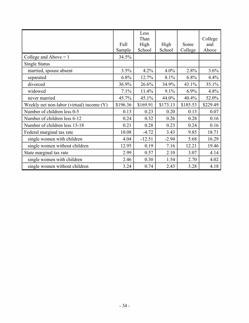
- 34 -

Full Sample

Less Than High

School High

School Some

College

College and

Above College and Above = 1 34.5% Single Status married, spouse absent 3.5% 4.2% 4.0% 2.8% 3.6% separated 6.8% 12.7% 8.1% 6.8% 4.4% divorced 36.9% 26.6% 34.9% 43.1% 35.1% widowed 7.1% 11.4% 9.1% 6.9% 4.8% never married 45.7% 45.1% 44.0% 40.4% 52.0% Weekly net non-labor (virtual) income (Y) $196.36 $169.91 $173.13 $185.53 $229.49 Number of children less 0-5 0.13 0.23 0.20 0.13 0.07 Number of children less 6-12 0.24 0.32 0.26 0.28 0.16 Number of children less 13-18 0.21 0.28 0.23 0.24 0.16 Federal marginal tax rate 10.08 -4.72 3.43 9.85 18.71 single women with children 4.04 -12.51 -2.94 5.68 16.29 single women without children 12.95 0.19 7.16 12.21 19.46 State marginal tax rate 2.99 0.57 2.10 3.07 4.14 single women with children 2.46 0.30 1.54 2.70 4.02 single women without children 3.24 0.74 2.43 3.28 4.18

- 35 -

Table 3 Estimated elasticities and marginal utilities, married and single families.

Full Sample

Husband (or single

head) Less Than High

School

Husband (or single

head) High

School

Husband (or single

head) Some

College

Husband (or single

head) College

and Above

Husband Elasticities Own wage elasticity 0.052 0.142 0.093 0.096 -0.003 Cross wage elasticity -0.066 -0.081 -0.054 -0.055 -0.063 Income elasticity -0.027 -0.034 -0.034 -0.023 -0.025 Participation own wage elasticity 0.009 0.071 0.023 0.018 0.000 Participation cross wage elasticity -0.010 -0.045 -0.014 -0.011 -0.003 Participation income elasticity -0.005 -0.017 -0.010 -0.005 -0.001

Wife Elasticities

Own wage elasticity 0.280 0.675 0.294 0.243 0.259 Cross wage elasticity -0.102 -0.168 -0.081 -0.080 -0.106 Income elasticity -0.029 -0.064 -0.033 -0.026 -0.027 Participation own wage elasticity 0.192 1.065 0.216 0.140 0.159 Participation cross wage elasticity -0.068 -0.239 -0.057 -0.046 -0.065 Participation income elasticity -0.019 -0.090 -0.025 -0.014 -0.017

Married Families Marginal Utilities MU wrt husband's non-market time 5.61 11.20 8.51 7.02 2.93 MU wrt wife's non-market time 4.23 7.71 6.62 5.71 2.08 MU wrt income 0.30 0.93 0.53 0.41 0.12

Single Men Elasticities and MUs Own wage elasticity 0.217 0.924 0.393 0.182 -0.046 Income elasticity -0.072 -0.136 -0.062 -0.067 -0.023 Participation own wage elasticity 0.032 0.518 0.098 0.025 -0.002 Participation income elasticity -0.010 -0.049 -0.013 -0.009 -0.001 MU wrt non-market time 132.51 355.51 115.97 137.78 4.30 MU wrt income 8.50 49.13 9.05 8.65 0.19

Single Women Elasticities and MUs Own wage elasticity 0.225 0.634 0.492 0.130 -0.015

- 36 -

Full Sample

Husband (or single

head) Less Than High

School

Husband (or single

head) High

School

Husband (or single

head) Some

College

Husband (or single

head) College

and Above

Income elasticity -0.070 -0.050 -0.062 -0.058 -0.034 Participation own wage elasticity 0.051 0.767 0.199 0.036 0.000 Participation income elasticity -0.014 -0.031 -0.021 -0.015 -0.001 MU wrt non-market time 67.57 55.48 81.42 45.15 8.91 MU wrt income 4.95 8.68 8.10 3.23 0.44

- 37 -

Table 4 Average welfare cost of a negative shock to employment by family type and education, share of total annual income in brackets.

Include families with non-employed

members

Families with at least one employed

member

All families $1,156 [1.74%]

$1,298 [1.95%]

Less than high school $454 [0.69%]

$639 [1.36%]

High school $898 [1.50%]

$1, 61 [1.77%]

Some college $1,019 [1.55%]

$1,145 [1.74%]

College or more $2,223 [2.81%]

$2,305 [2.92%]

Married families $1,944 [2.85%]

$2,021 [2.96%]

Single families $131 [0.29%]

$164 [0.36%]

married, spouse-not-present $153 [0.32%]

$183 [0.38%]

separated $125 [0.31%]

$168 [0.42%]

divorced $128 [0.26%]

$163 [0.33]

widowed $75 [0.16%]

$116 [0.24%]

never married $139 [0.32%]

$168 [0.39]

Note: Education refers to single head of household or husband education for married families. Full sample estimates are used to report results for the full sample and the education specific estimates are used to report results by education group.

- 38 -

Table 5 Average equivalent price level change estimated by family type and education.

Include families with non-employed

members

Families with at least one employed

member All families 1.82% 2.04%

Less than high school 1.13% 1.60%

High school 1.53% 1.81%

Some college 1.64% 1.84%

College or more 2.85% 2.95%

Married families 2.98% 3.10%

Single families 0.30% 0.38%

married, spouse-not-present 0.34% 0.41%

separated 0.30% 0.40%

divorced 0.28% 0.35%

widowed 0.18% 0.27%

never married 0.33% 0.40%

Note: Education refers to single head of household or husband education for married families. Full sample estimates are used to report results for the full sample and the education specific estimates are used to report results by education group.

- 39 -

Figure 1 Comparison of intensive margin elasticity estimates with the literature. (a) Husband's (men's) elasticities

(b) Wife's (women's) elasticities

Notes: Sources of literature estimates are Devereux (2004); Hotchkiss, Moore, and Rios-Avila (2012); Hotchkiss, Kassis, and Moore (1997); Heim (2009); Blau and Kahn (2007); Triest (1990); Pencavel (2002); Ransom (1987); Blundell and Macurdy (1999); Kumar (2009); Bishop, Heim, and Mihaly (2009); Imai and Keane (2004); and Chetty (2012). Also see Keane (2011) and McClelland and Mok (2012) Many fewer sources provide estimates for participation elasticities, but ours fall within the literature bounds (available upon request).

- 40 -

Figure 2 Comparing welfare losses from a price shock vs. an unemployment shock across the income distribution, full sample averages. (a) Welfare loss from equivalent price level change

(b) Welfare loss from 1pp increase in the aggregate unemployment rate (% of total income)

(c) Ratio of welfare loss from a price level change vs. welfare loss from unemployment shock

Note: Percent of the sample noted by dashed lines at maximum household income for those in the bottom 20%, the sample median, and the min household income for those in the top 20%. Comparable 2015 median household incomes reported for the U.S. by the Census Bureau can be found here: https://goo.gl/XkzVMR.

01

23

Wel

fare

loss

equ

ival

ent s

hock

to p

rices

(%)

020000

4000060000

80000100000

120000140000

160000180000

200000

Total Annual Income

95% CI lpoly smoothkernel = epanechnikov, degree = 0, bandwidth = 6000, pwidth = 1635.98

01

23

Wel

fare

loss

from

UR

sho

ck, %

of t

otal

inco

me

020000

4000060000

80000100000

120000140000

160000

Total Annual Income

95% CI lpoly smoothkernel = epanechnikov, degree = 0, bandwidth = 6000, pwidth = 2032.55

0.5

11.

5Pr

ice

shoc

k/U

nem

ploy

men

t sho

ck tr

adeo

ff

020000

4000060000

80000100000

120000140000

160000

Total Annual Income

95% CI lpoly smoothkernel = epanechnikov, degree = 0, bandwidth = 6000, pwidth = 1053.16

- A1 -

Appendix A: Estimation Issues -- obtaining reasonable labor supply elasticities

The simulations detailed in Section 2 are only possible to the extent to which we are able

to obtain realistic estimates of labor supply elasticities through which the change in family

welfare is calculated. This appendix discusses a number of issues well-known to the literature

related to the estimation of those labor supply elasticities and the implications of those issues to

the problem at hand. Many of the caveats, warnings, solutions, and implications related to this

specific model were first detailed in Hotchkiss et al (2012).

First of all, the stochastic errors accounted for in equation (7) represent errors in

optimization -- observed hours do not exactly reflect desired hours. Keane (2011) points out that

there may exist measurement error in observed wages and non-labor income. This classical

measurement error may bias elasticity estimates toward zero. Heim (2009), using a methodology

most similar to the one used here, presents results showing that accounting for measurement

error produces elasticities practically identical to when it is not accounted for. A typical strategy

to mitigate the introduction of measurement error on wages per hour has been to restrict the

sample to hourly paid workers. Unfortunately, restricting the sample to hourly workers reduces

the sample size too much. Instead, we construct the person's hourly wage using information

about weekly earnings and usual weekly hours. This means our wage estimate might suffer from

what Keane refers to as "denominator bias," which will have the tendency of biasing labor

supply elasticities downward.

Keane (2011) also identifies two potential sources of endogeneity. First, it is reasonable

to expect that observed wages and non-labor income are correlated with a person's taste for work

(reflected through hours of work). Both fixed effects and instrumental variables have been used

to resolve this issue, but are simply not possible in this case since we do not have panel data and

because of the highly non-linear nature of the labor supply functions. In addition to the inclusion

- A2 -

of variables expected to affect the taste for work (e.g., children), we expect that the inclusion of

spousal variables (through the estimation of joint labor supply) will help to remove additional

sources of correlation from the error term (i.e., because of positive assortative mating, people

with similar taste for work will be married to each other; see Lam 1988 and Herrnstein and

Murray 1994). In addition, we abstract from the progressivity of the tax structure by using net

wages and "linearizing" the budget constraint (see Hall 1973), which is valid if preferences are

strictly convex. This means that family members would make the same hours choice facing this

linearized budget constraint that they would have made facing the nonlinear budget constraint.

This assumption of strictly convex preferences can be tested by analyzing the second order

conditions of the maximization problem, which are akin to the internal consistency conditions

established by (Amemiya 1974, 1006). Using the nomenclature presented in equations 5 and 6,

the conditions imply that Ω! < 0;  Ω! < 0 and Ω!Ω! > Ω! ∗ Ω!, which are found to be true for

all the models estimated here. If this assumption is binding, Keane points out that labor supply

elasticities will be biased in a negative direction. Aaronson and French (2009) illustrate only a

very slight downward bias when progressivity of the tax system is not taken into account.

An additional concern Keane (2011) identifies in the literature is making sure the

hours/wage combinations observed in the data are coming off workers' labor supply curve, rather

than off employers' labor demand curve. Identification of the labor supply relationship boils

down to including regressors (determinants of hours) that reflect the demand for a person's skills

(thus determine the observed wage) that are not reflective of that person's taste for work. Toward

that end, we include an indicator for race that could affect observed wage through employer

discrimination, but, ceteris paribus (e.g., controlling for education), should not affect taste for

work.

- A3 -

Further, the issue of the presence of fixed costs of working is raised by Apps and Rees

(2009). We only marginally control for fixed costs by including the presence of children in the

determination of hours. However, Heim (2009) presents results showing that once demographics

are controlled for, additional consideration of fixed costs only very slightly impacts estimates of

the parameters of the utility function (Heim, Table 3).

As is seen in Section 4, the simplifications that we've made because of the complexity of

the model do not harm our goal of obtaining reasonable labor supply elasticities with which to

perform the simulations in this paper.

- B1 -

Appendix B: First order conditions of utility maximization problem and labor supply equations. The quadratic functional form as presented in equation (4) in the text can also be written

in the following form:

𝑈 𝑍 = 𝑎! 𝐿! + 𝑎! 𝐿! + 𝑎! 𝐶 − !!𝑏!! 𝐿! ! − !

!𝑏!! 𝐿! ! − !

!𝑏!! 𝐶 ! − 𝑏!"𝐿!𝐿! − 𝑏!"𝐿!𝐶 − 𝑏!"𝐿!𝐶 (A1)

Where 𝐿! = 𝑇 − ℎ!; 𝐿! = 𝑇 − ℎ!;𝑎𝑛𝑑,𝐶 = 𝑤!ℎ! + 𝑤!ℎ! + 𝑌

This becomes an unconstrained utility maximization problem which depends on the working

hours ℎ! and ℎ!, assuming that Y (non-labor income) is exogenous. The corresponding first order

conditions become:

!"!!!

= 𝑎!∗ + 𝑎!∗𝑤! − 𝑏!!ℎ! − 𝑏!!𝑤! 𝑤!ℎ! + 𝑤!ℎ! + 𝑌 − 𝑏!"ℎ! + 𝑏!" 2𝑤!ℎ! + 𝑤!ℎ! + 𝑌 + 𝑏!"𝑤!ℎ! = 0 (A2)

!"!!!

= 𝑎!∗ + 𝑎!∗𝑤! − 𝑏!!ℎ! − 𝑏!!𝑤! 𝑤!ℎ! + 𝑤!ℎ! + 𝑌 − 𝑏!"ℎ! + 𝑏!" 𝑤!ℎ! + 2𝑤!ℎ! + 𝑌 + 𝑏!"𝑤!ℎ! = 0 (A3)

There is no need to specify a time endowment (T) in order to estimate the labor supply functions

because 𝑎!∗, 𝑎!∗ , and 𝑎!∗ are re-parameterized functions of T and Y. This re-parameterization is

necessary for identification of the labor supply equations. It is through these starred parameters

that differences in tastes across families are allowed to enter. Specifically,

𝑎!∗ = 𝑋!Γ! and 𝑎!∗ = 𝑋!Γ!

where 𝑋! and 𝑋! are vectors of individual and family characteristics and Γ! and Γ! are parameters

to be estimated.

Using equations (A2) and (A3), we can solve the system obtaining the values of ℎ! and

ℎ! that maximize the utility function, in the following way:

Ω!ℎ!∗ + Ω!ℎ!∗ + Ω! = 0 (A4)

Ω!ℎ!∗ + Ω!ℎ!∗ + Ω! = 0, where, (A5)

Ω! = 2𝑏!"𝑤! − 𝑏!! − 𝑏!!𝑤!!; (A6)

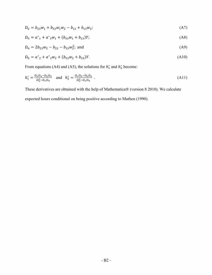
- B2 -

Ω! = 𝑏!"𝑤! + 𝑏!!𝑤!𝑤! − 𝑏!" + 𝑏!"𝑤!; (A7)

Ω! = 𝑎∗! + 𝑎∗!𝑤! + 𝑏!!𝑤! + 𝑏!" 𝑌; (A8)

Ω! = 2𝑏!"𝑤! − 𝑏!! − 𝑏!!𝑤!!;  and (A9)

Ω! = 𝑎∗! + 𝑎∗!𝑤! + 𝑏!!𝑤! + 𝑏!" 𝑌. (A10)

From equations (A4) and (A5), the solutions for ℎ!∗ and ℎ!∗ become:

ℎ!∗ =!!!!!!!!!!!!!!!!!

and ℎ!∗ =!!!!!!!!!!!!!!!!!

. (A11)

These derivatives are obtained with the help of Mathematica® (version 8 2010). We calculate

expected hours conditional on being positive according to Muthen (1990).

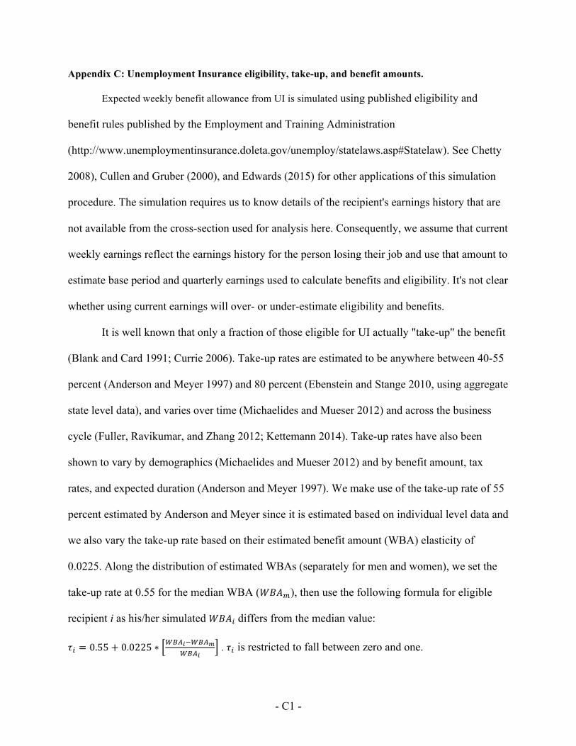
- C1 -

Appendix C: Unemployment Insurance eligibility, take-up, and benefit amounts.

Expected weekly benefit allowance from UI is simulated using published eligibility and

benefit rules published by the Employment and Training Administration

(http://www.unemploymentinsurance.doleta.gov/unemploy/statelaws.asp#Statelaw). See Chetty

2008), Cullen and Gruber (2000), and Edwards (2015) for other applications of this simulation

procedure. The simulation requires us to know details of the recipient's earnings history that are

not available from the cross-section used for analysis here. Consequently, we assume that current

weekly earnings reflect the earnings history for the person losing their job and use that amount to

estimate base period and quarterly earnings used to calculate benefits and eligibility. It's not clear

whether using current earnings will over- or under-estimate eligibility and benefits.

It is well known that only a fraction of those eligible for UI actually "take-up" the benefit

(Blank and Card 1991; Currie 2006). Take-up rates are estimated to be anywhere between 40-55

percent (Anderson and Meyer 1997) and 80 percent (Ebenstein and Stange 2010, using aggregate

state level data), and varies over time (Michaelides and Mueser 2012) and across the business

cycle (Fuller, Ravikumar, and Zhang 2012; Kettemann 2014). Take-up rates have also been

shown to vary by demographics (Michaelides and Mueser 2012) and by benefit amount, tax

rates, and expected duration (Anderson and Meyer 1997). We make use of the take-up rate of 55

percent estimated by Anderson and Meyer since it is estimated based on individual level data and

we also vary the take-up rate based on their estimated benefit amount (WBA) elasticity of

0.0225. Along the distribution of estimated WBAs (separately for men and women), we set the

take-up rate at 0.55 for the median WBA (𝑊𝐵𝐴!), then use the following formula for eligible

recipient i as his/her simulated 𝑊𝐵𝐴! differs from the median value:

𝜏! = 0.55 + 0.0225 ∗ !"#!!!"#!!"#!

. 𝜏! is restricted to fall between zero and one.

- D1 -

Appendix D: Maximum likelihood estimation results. Table D.1 Maximum likelihood parameter estimates for married families.

Full Sample

Husband Less Than

High School Husband

High School

Husband Some

College

Husband College or

More a1: Husband Age 2.122* 2.013* 1.991* 2.675* 2.033* (0.120) (0.550) (0.251) (0.245) (0.178) Age^2 -0.0278* -0.0290* -0.0277* -0.0341* -0.0255* (0.00135) (0.00629) (0.00284) (0.00275) (0.00199) Black -2.356* 3.015+ -3.472* -3.977* -1.785* (0.332) (1.428) (0.726) (0.710) (0.445) Education (excluded=Less than High School) High School 5.245*

(0.574) Some College 7.107* (0.586) College 11.89* (0.605) nkids 0-5 -0.169 1.980^ -0.296 0.0281 -0.535^

(0.243) (1.098) (0.588) (0.516) (0.303) nkids 6-12 0.0112 1.310 -0.0943 -0.453 -0.312 (0.202) (0.853) (0.450) (0.428) (0.270) nkids 13-18 1.041* 2.257+ 0.626 0.381 0.924* (0.243) (1.025) (0.532) (0.514) (0.325) Constant -7.440* -13.04 0.668 -14.02* 6.614^ (2.579) (11.62) (5.218) (5.148) (3.805) a2: Wife Age 0.462* 0.00951 0.485* 0.921* 0.325* (0.0503) (0.111) (0.123) (0.164) (0.0566) Age^2 -0.00631* -0.000618 -0.00668* -0.0119* -0.00434* (0.000627) (0.00131) (0.00150) (0.00200) (0.000716) Black -0.806* 0.215 -1.454* 0.0779 -0.712* (0.120) (0.313) (0.353) (0.334) (0.130) Education (excluded=Less than High School) High School 2.430* 0.497 3.821* 2.753* 0.871 (0.277) (0.351) (0.779) (0.984) (0.550) Some College 3.098* 0.742^ 5.090* 4.296* 0.862

- D2 -

Full Sample

Husband Less Than

High School Husband

High School

Husband Some

College

Husband College or

More (0.311) (0.427) (0.931) (1.061) (0.540) College 3.883* -1.507+ 5.991* 6.539* 1.461* (0.357) (0.721) (1.081) (1.288) (0.558) nkids 0-5 -1.511* -0.0800 -1.857* -2.318* -0.970* (0.135) (0.262) (0.348) (0.390) (0.148) nkids 6-12 -0.727* -0.130 -0.793* -0.846* -0.551* (0.0855) (0.198) (0.216) (0.233) (0.0969) nkids 13-18 -0.0676 0.835* 0.285 -0.310 -0.212* (0.0803) (0.256) (0.226) (0.250) (0.0803) Constant -7.282* -7.423* -11.43* -14.30* -3.239* (0.945) (2.765) (2.672) (3.106) (1.071) a3 0.524* 1.408* 0.852* 0.623* 0.286* (0.0308) (0.254) (0.0920) (0.0699) (0.0274) b12 0.0298* 0.00427 -0.0469^ 0.0401 0.0399+ (0.00918) (0.0265) (0.0265) (0.0254) (0.0160) b13 -0.00264* -0.00331^ -0.00383* -0.00159* -0.00238* (0.000202) (0.00174) (0.000587) (0.000449) (0.000212) b22 0.231* 0.139* 0.332* 0.389* 0.126* (0.0166) (0.0256) (0.0431) (0.0500) (0.0178) b23 -0.000207+ 0.000822 -0.000531 -0.000185 -0.000109^ (0.0000882) (0.000778) (0.000354) (0.000276) (0.0000650) b33 0.0000792* 0.000500* 0.000143* 0.000108* 0.0000338* (0.00000670) (0.000127) (0.0000233) (0.0000168) (0.00000505) drho 0.0219^ 0.124* 0.0825* 0.00210 -0.0281 (0.0117) (0.0470) (0.0230) (0.0228) (0.0183) s1 17.94* 22.52* 19.58* 19.16* 15.10* (0.0993) (0.505) (0.216) (0.211) (0.126) s2 23.94* 27.69* 24.29* 22.63* 23.61* (0.156) (0.822) (0.311) (0.281) (0.237) N 20163 1502 5401 5233 8027 LL -149921.9 -9517.4 -39636.0 -39446.3 -60673.0

Notes: Standard errors are in brackets. *, +, ^ => significant at the 99, 95, and 90 percent confidence levels, respectively.

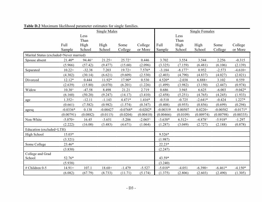
- D3 -

Table D.2 Maximum likelihood parameter estimates for single families. Single Males Single Females

Full Sample

Less Than High School

High School

Some College

College or More

Full Sample

Less Than High School

High School

Some College

College or More

Marital Status (excluded=Never married) Spouse absent 21.40* 94.46^ 21.25+ 25.72^ 0.446 3.702 3.554 3.544 2.256 -0.315

(5.966) (57.42) (9.477) (15.60) (2.096) (3.325) (7.159) (6.481) (6.106) (2.139)

Separated 10.22+ -32.38 7.203 19.72+ 7.576* -3.184 -8.177^ 0.952 -2.573 -4.610+ (4.302) (30.14) (6.621) (9.609) (2.530) (2.403) (4.790) (4.837) (4.027) (2.021) Divorced 12.12* 0.444 11.92* 17.90* 0.530 4.520* -2.038 6.888+ 3.102 0.559 (2.639) (15.80) (4.070) (6.201) (1.226) (1.499) (3.982) (3.150) (2.447) (0.974) Widow 10.30^ -47.58 8.498 21.21 2.719 0.686 3.945 6.625 -6.003 -9.042* (6.160) (50.20) (9.247) (14.17) (3.410) (2.458) (5.251) (4.765) (4.245) (1.933) age 1.352+ -12.11 -1.143 4.471* 1.416* -0.510 -0.725 -2.641* -0.424 1.227* (0.661) (7.582) (0.982) (1.574) (0.347) (0.408) (0.955) (0.856) (0.699) (0.294) agesq -0.0336* 0.138 -0.00427 -0.0768* -0.0202* -0.00319 0.00507 0.0220+ -0.00582 -0.0171* (0.00791) (0.0882) (0.0115) (0.0204) (0.00410) (0.00466) (0.0109) (0.00974) (0.00798) (0.00335) Non-White -5.070+ 16.45 -3.651 -5.206 -2.065^ -3.638* 6.512+ -4.878^ -5.918* -1.297 (2.222) (16.00) (3.483) (4.671) (1.064) (1.287) (3.049) (2.727) (2.188) (0.878) Education (excluded=LTH)

High School 15.03*

9.526*

(3.321)

(1.987)

Some College 23.46*

22.23*

(3.830)

(2.247)

College and Grad School 52.76*

43.59*

(5.938)

(3.240)

# Children 0-5 14.91+ 107.1 18.68+ -1.479 -5.527 -5.018* -4.051 -6.390+ -6.461* -4.150*

(6.082) (67.79) (8.733) (11.71) (5.174) (1.375) (2.806) (2.603) (2.490) (1.305)

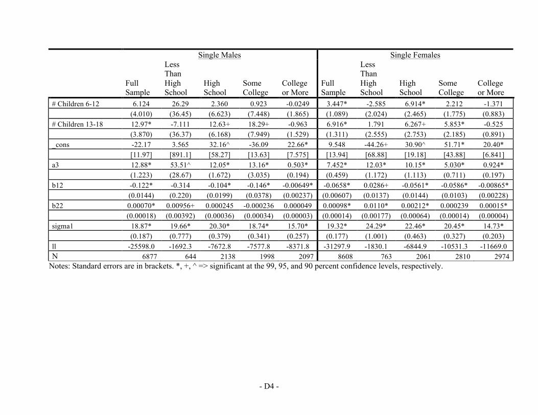
- D4 -

Single Males Single Females

Full Sample

Less Than High School

High School

Some College

College or More

Full Sample

Less Than High School

High School

Some College

College or More

# Children 6-12 6.124 26.29 2.360 0.923 -0.0249 3.447* -2.585 6.914* 2.212 -1.371

(4.010) (36.45) (6.623) (7.448) (1.865) (1.089) (2.024) (2.465) (1.775) (0.883)

# Children 13-18 12.97* -7.111 12.63+ 18.29+ -0.963 6.916* 1.791 6.267+ 5.853* -0.525

(3.870) (36.37) (6.168) (7.949) (1.529) (1.311) (2.555) (2.753) (2.185) (0.891)

_cons -22.17 3.565 32.16^ -36.09 22.66* 9.548 -44.26+ 30.90^ 51.71* 20.40* [11.97] [891.1] [58.27] [13.63] [7.575] [13.94] [68.88] [19.18] [43.88] [6.841] a3 12.88* 53.51^ 12.05* 13.16* 0.503* 7.452* 12.03* 10.15* 5.030* 0.924*

(1.223) (28.67) (1.672) (3.035) (0.194) (0.459) (1.172) (1.113) (0.711) (0.197)

b12 -0.122* -0.314 -0.104* -0.146* -0.00649* -0.0658* 0.0286+ -0.0561* -0.0586* -0.00865*

(0.0144) (0.220) (0.0199) (0.0378) (0.00237) (0.00607) (0.0137) (0.0144) (0.0103) (0.00228)

b22 0.00070* 0.00956+ 0.000245 -0.000236 0.000049 0.00098* 0.0110* 0.00212* 0.000239 0.00015*

(0.00018) (0.00392) (0.00036) (0.00034) (0.00003) (0.00014) (0.00177) (0.00064) (0.00014) (0.00004)

sigma1 18.87* 19.66* 20.30* 18.74* 15.70* 19.32* 24.29* 22.46* 20.45* 14.73*

(0.187) (0.777) (0.379) (0.341) (0.257) (0.177) (1.001) (0.463) (0.327) (0.203)

ll -25598.0 -1692.3 -7672.8 -7577.8 -8371.8 -31297.9 -1830.1 -6844.9 -10531.3 -11669.0 N 6877 644 2138 1998 2097 8608 763 2061 2810 2974

Notes: Standard errors are in brackets. *, +, ^ => significant at the 99, 95, and 90 percent confidence levels, respectively.

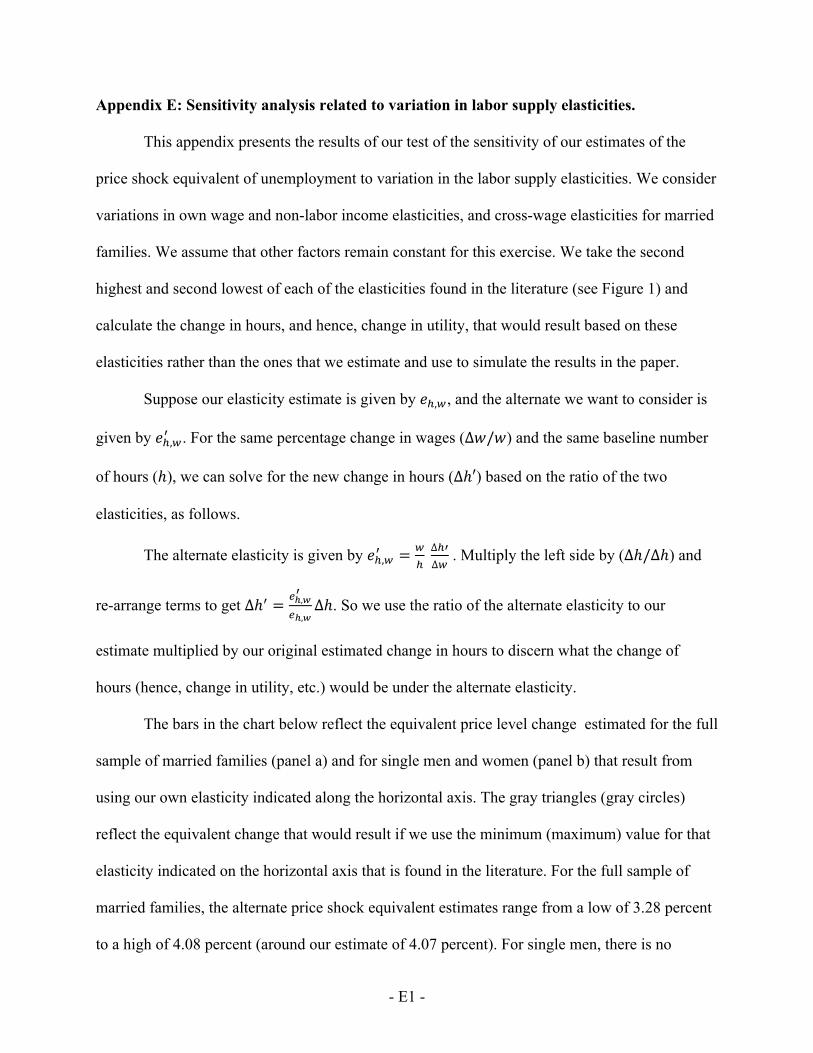
- E1 -

Appendix E: Sensitivity analysis related to variation in labor supply elasticities. This appendix presents the results of our test of the sensitivity of our estimates of the

price shock equivalent of unemployment to variation in the labor supply elasticities. We consider

variations in own wage and non-labor income elasticities, and cross-wage elasticities for married

families. We assume that other factors remain constant for this exercise. We take the second

highest and second lowest of each of the elasticities found in the literature (see Figure 1) and

calculate the change in hours, and hence, change in utility, that would result based on these

elasticities rather than the ones that we estimate and use to simulate the results in the paper.

Suppose our elasticity estimate is given by 𝑒!,!, and the alternate we want to consider is

given by 𝑒!,!! . For the same percentage change in wages (∆𝑤/𝑤) and the same baseline number

of hours (ℎ), we can solve for the new change in hours (∆ℎ′) based on the ratio of the two

elasticities, as follows.

The alternate elasticity is given by 𝑒!,!! = !!  ∆!"∆!

. Multiply the left side by (Δℎ/Δℎ) and

re-arrange terms to get ∆ℎ! = !!,!!

!!,!Δℎ. So we use the ratio of the alternate elasticity to our

estimate multiplied by our original estimated change in hours to discern what the change of

hours (hence, change in utility, etc.) would be under the alternate elasticity.

The bars in the chart below reflect the equivalent price level change estimated for the full

sample of married families (panel a) and for single men and women (panel b) that result from

using our own elasticity indicated along the horizontal axis. The gray triangles (gray circles)

reflect the equivalent change that would result if we use the minimum (maximum) value for that

elasticity indicated on the horizontal axis that is found in the literature. For the full sample of

married families, the alternate price shock equivalent estimates range from a low of 3.28 percent

to a high of 4.08 percent (around our estimate of 4.07 percent). For single men, there is no

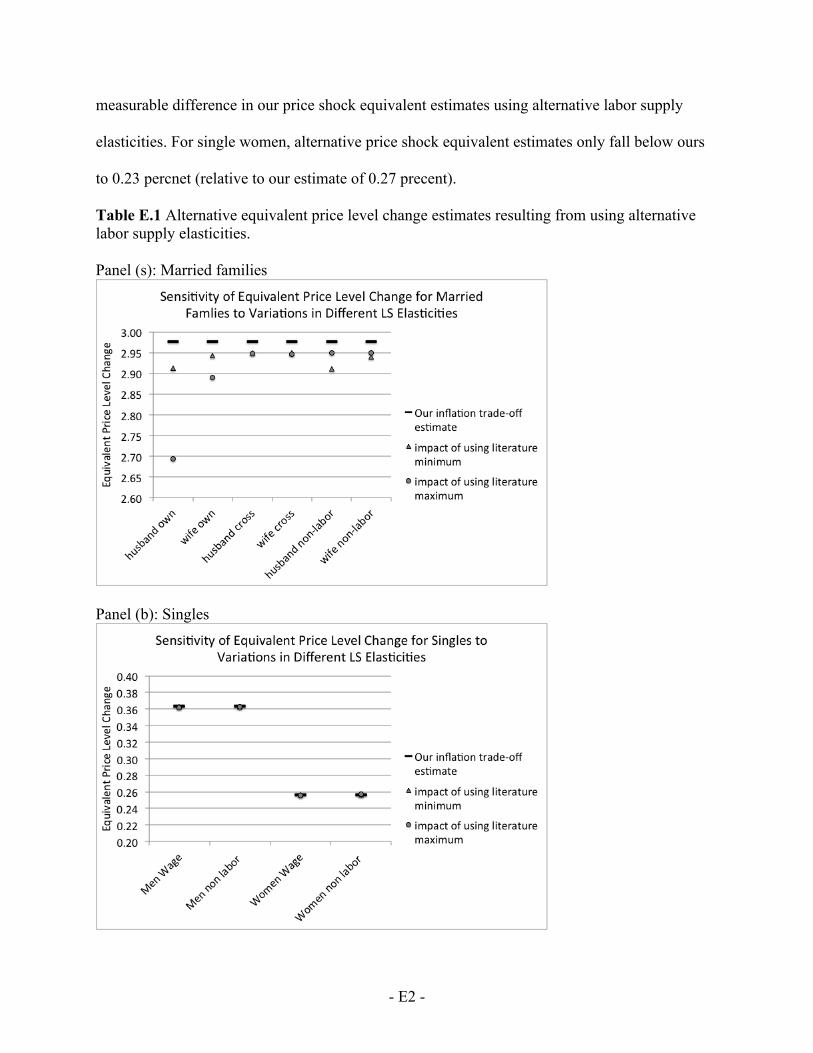
- E2 -

measurable difference in our price shock equivalent estimates using alternative labor supply

elasticities. For single women, alternative price shock equivalent estimates only fall below ours

to 0.23 percnet (relative to our estimate of 0.27 precent).

Table E.1 Alternative equivalent price level change estimates resulting from using alternative labor supply elasticities. Panel (s): Married families

Panel (b): Singles

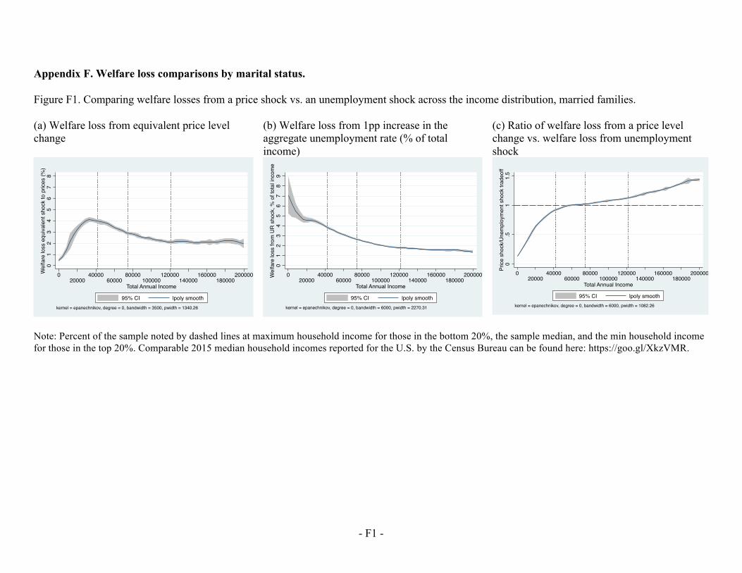
- F1 -

Appendix F. Welfare loss comparisons by marital status.

Figure F1. Comparing welfare losses from a price shock vs. an unemployment shock across the income distribution, married families. (a) Welfare loss from equivalent price level change

(b) Welfare loss from 1pp increase in the aggregate unemployment rate (% of total income)

(c) Ratio of welfare loss from a price level change vs. welfare loss from unemployment shock

Note: Percent of the sample noted by dashed lines at maximum household income for those in the bottom 20%, the sample median, and the min household income for those in the top 20%. Comparable 2015 median household incomes reported for the U.S. by the Census Bureau can be found here: https://goo.gl/XkzVMR.

01

23

45

67

8W

elfa

re lo

ss e

quiv

alen

t sho

ck to

pric

es (%

)

020000

4000060000

80000100000

120000140000

160000180000

200000

Total Annual Income

95% CI lpoly smoothkernel = epanechnikov, degree = 0, bandwidth = 3500, pwidth = 1340.26

01

23

45

67

89

Wel

fare

loss

from

UR

sho

ck, %

of t

otal

inco

me

020000

4000060000

80000100000

120000140000

160000180000

200000

Total Annual Income

95% CI lpoly smoothkernel = epanechnikov, degree = 0, bandwidth = 6000, pwidth = 2270.31

0.5

11.

5Pr

ice

shoc

k/U

nem

ploy

men

t sho

ck tr

adeo

ff

020000

4000060000

80000100000

120000140000

160000180000

200000

Total Annual Income

95% CI lpoly smoothkernel = epanechnikov, degree = 0, bandwidth = 6000, pwidth = 1082.26

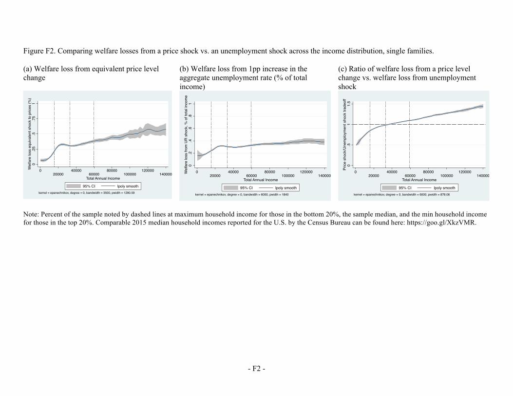
- F2 -

Figure F2. Comparing welfare losses from a price shock vs. an unemployment shock across the income distribution, single families. (a) Welfare loss from equivalent price level change

(b) Welfare loss from 1pp increase in the aggregate unemployment rate (% of total income)

(c) Ratio of welfare loss from a price level change vs. welfare loss from unemployment shock

Note: Percent of the sample noted by dashed lines at maximum household income for those in the bottom 20%, the sample median, and the min household income for those in the top 20%. Comparable 2015 median household incomes reported for the U.S. by the Census Bureau can be found here: https://goo.gl/XkzVMR.

0.2

5.5

.75

1W

elfa

re lo

ss e

quiv

alen

t sho

ck to

pric

es (%

)

020000

4000060000

80000100000

120000140000

Total Annual Income

95% CI lpoly smoothkernel = epanechnikov, degree = 0, bandwidth = 3500, pwidth = 1290.59

0.2

.4.6

.81

Wel

fare

loss

from

UR

sho

ck, %

of t

otal

inco

me

020000

4000060000

80000100000

120000140000

Total Annual Income

95% CI lpoly smoothkernel = epanechnikov, degree = 0, bandwidth = 6000, pwidth = 1840

0.5

11.

5Pr

ice

shoc

k/U

nem

ploy

men

t sho

ck tr

adeo

ff

020000

4000060000

80000100000

120000140000

Total Annual Income

95% CI lpoly smoothkernel = epanechnikov, degree = 0, bandwidth = 6000, pwidth = 878.06