The Video Encyclopedia of Physics Demonstrationsjedlik.phy.bme.hu/f29/dvd/01_brochure.pdf · 2005. 5. 3. · Physics Vade Mecum (American Institute of Physics, New York, 1989),

TheVideoEncyclopedia

ofPhysicsDemonstrations™

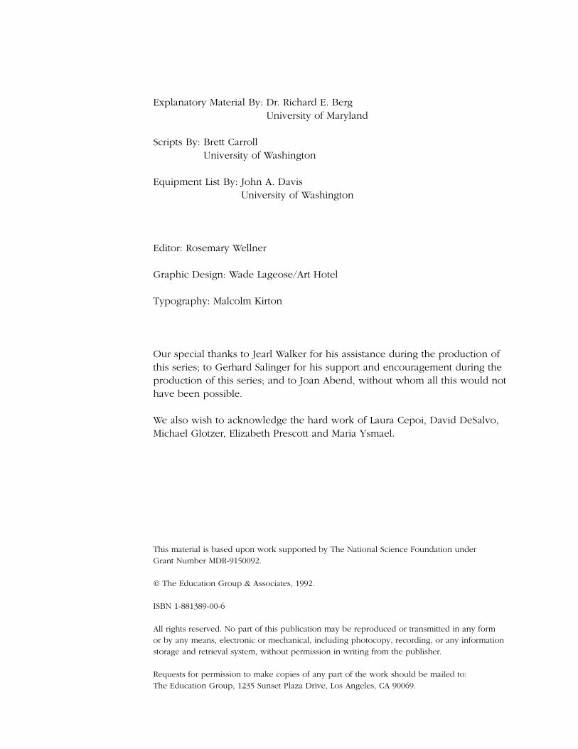
Explanatory Material By: Dr. Richard E. BergUniversity of Maryland

Scripts By: Brett CarrollUniversity of Washington

Equipment List By: John A. DavisUniversity of Washington

Editor: Rosemary Wellner

Graphic Design: Wade Lageose/Art Hotel

Typography: Malcolm Kirton

Our special thanks to Jearl Walker for his assistance during the production ofthis series; to Gerhard Salinger for his support and encouragement during theproduction of this series; and to Joan Abend, without whom all this would nothave been possible.

We also wish to acknowledge the hard work of Laura Cepoi, David DeSalvo,Michael Glotzer, Elizabeth Prescott and Maria Ysmael.

This material is based upon work supported by The National Science Foundation under Grant Number MDR-9150092.

© The Education Group & Associates, 1992.

ISBN 1-881389-00-6

All rights reserved. No part of this publication may be reproduced or transmitted in any form or by any means, electronic or mechanical, including photocopy, recording, or any informationstorage and retrieval system, without permission in writing from the publisher.

Requests for permission to make copies of any part of the work should be mailed to: The Education Group, 1235 Sunset Plaza Drive, Los Angeles, CA 90069.

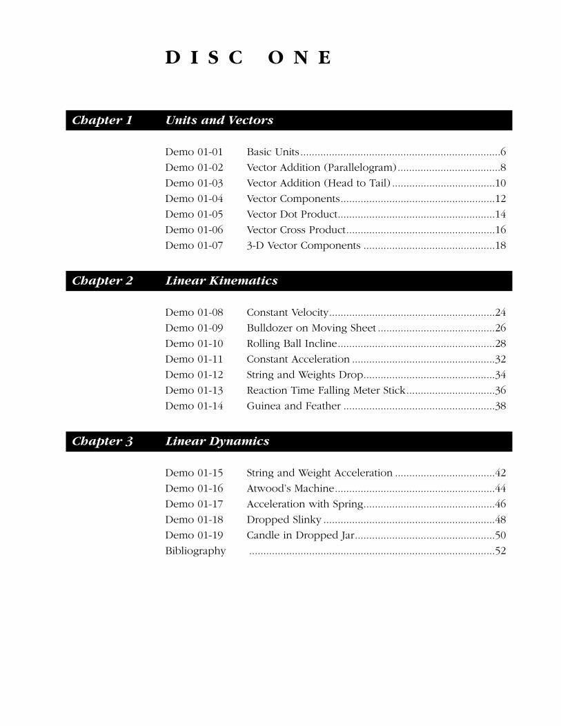
D I S C O N E

Chapter 1 Units and Vectors

Demo 01-01 Basic Units......................................................................6

Demo 01-02 Vector Addition (Parallelogram)....................................8

Demo 01-03 Vector Addition (Head to Tail) ....................................10

Demo 01-04 Vector Components......................................................12

Demo 01-05 Vector Dot Product.......................................................14

Demo 01-06 Vector Cross Product....................................................16

Demo 01-07 3-D Vector Components ..............................................18

Chapter 2 Linear Kinematics

Demo 01-08 Constant Velocity..........................................................24

Demo 01-09 Bulldozer on Moving Sheet .........................................26

Demo 01-10 Rolling Ball Incline.......................................................28

Demo 01-11 Constant Acceleration ..................................................32

Demo 01-12 String and Weights Drop..............................................34

Demo 01-13 Reaction Time Falling Meter Stick...............................36

Demo 01-14 Guinea and Feather .....................................................38

Chapter 3 Linear Dynamics

Demo 01-15 String and Weight Acceleration ...................................42

Demo 01-16 Atwood’s Machine........................................................44

Demo 01-17 Acceleration with Spring..............................................46

Demo 01-18 Dropped Slinky ............................................................48

Demo 01-19 Candle in Dropped Jar.................................................50

Bibliography ......................................................................................52

C H A P T E R 1

U N I T S A N D V E C T O R S

5

† Herbert L. Anderson, Editor-in-Chief, A Physicist’s Desk Reference, The Second Edition ofPhysics Vade Mecum (American Institute of Physics, New York, 1989), page 5.

The three basic quantities from which most other mechanical units are derivedare mass, length, and time. Physicists commonly prefer to use the system ofunits known as SI (Système Internationale in French), or metric units. SI unitsfor these quantities are the kilogram for mass, the meter for length, and thesecond for time. According to the reference volume A Physicist’s DeskReference,† these units are defined as follows:

meter (symbol m) : “The meter is the length of path travelled by light in vac-uum during the time interval 1/299,792,458 of a second.”

kilogram (symbol kg) : “The kilogram is the unit of mass, it is equal to the massof the international prototype of the kilogram.” (The international prototype isa platinum-iridium cylinder kept at the BIPM in Sèvres, France.)

second (symbol s) : “The second is the duration of 9,192,631,770 periods of theradiation corresponding to the transition between the two hyperfine levels ofthe ground state of the cesium-133 atom.”

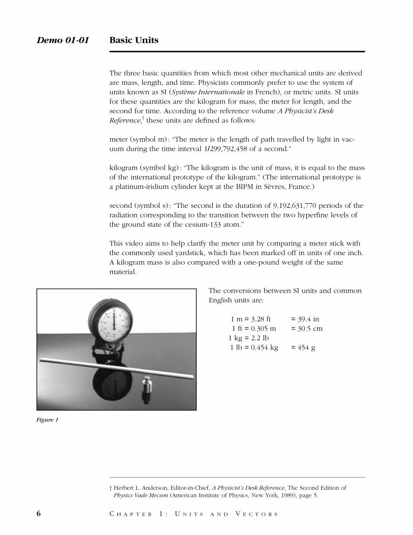
This video aims to help clarify the meter unit by comparing a meter stick withthe commonly used yardstick, which has been marked off in units of one inch.A kilogram mass is also compared with a one-pound weight of the samematerial.

The conversions between SI units and commonEnglish units are:

1 m = 3.28 ft = 39.4 in 1 ft = 0.305 m = 30.5 cm

1 kg = 2.2 lb1 lb = 0.454 kg = 454 g

Demo 01-01 Basic Units

6 C H A P T E R 1 : U N I T S A N D V E C T O R S

Figure 1

Equipment

1. 1-kilogram mass and a 1-pound mass to compare.2. 1 meter stick and 1 yardstick to compare.3. 1 clock with a 1-second sweep hand.

Physics makes use of a standard set of reference units for quantities such asmass, length, and time.

Here are examples of the standard units and their modern methods of deriva-tion.

The standard unit of mass is the kilogram, which can be calibrated only bycomparing it with a standard kilogram carefully maintained in a vault inFrance, or duplicates made from the standard.

The standard unit of length is the meter, which is now defined in terms of thedistance light travels in a specific time interval approximately equal to one 300millionth of a second.

For the purpose of comparison, here is the length of one yard. The standardunit of time is the second, which is defined as the time required for a precisenumber of periods of a type of radiation emitted by cesium atoms.

These three units combine to make up many of the other units commonlyused in physics.

Basic Units / Script Demo 01-01

C H A P T E R 1 : U N I T S A N D V E C T O R S 7

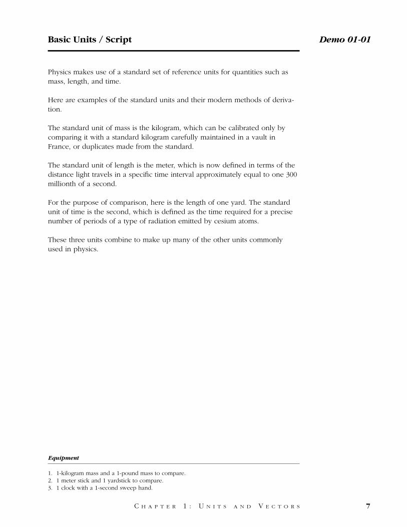
Vector addition can be carried out either graphically or mathematically bycomponents. This graphics demonstration illustrates the “parallelogram rule,”one method by which we can add vectors.

The two vectors to be added are translated without rotation so that their tailstouch, forming two sides of a parallelogram. The remaining sides of the paral-lelogram are then constructed parallel to the two vectors. We can then drawthe vector sum of the two original vectors from the point at which the two tailstouch to the corner of the parallelogram opposite that corner, as shown inFigure 1 and on the video for several different sets of vectors.

Demo 01-02 Vector Addition (Parallelogram)


B→ B

→C = A + B→→

→

A→

A→

B→

Figure 1

We’ll use these animated vector arrows to demonstrate the parallelogrammethod of adding vectors.

The vectors are positioned with their tails together, and a parallelogram isformed by putting in lines that are parallel to and equal in length to each ofthe vectors. The sum of the two vectors is the vector formed by drawing a linefrom the tails across to the opposite corner of the parallelogram. As the anglebetween the vectors changes, the magnitude of their sum changes from zero totwice the magnitude of either vector.

Here is the same sequence repeated with vectors of unequal length.

Vector Addition (Parallelogram) / Script Demo 01-02


Equipment

This demonstration is animated, but can be done with vector shapes mounted on magnets,which in turn adhere to a ferrous blackboard.

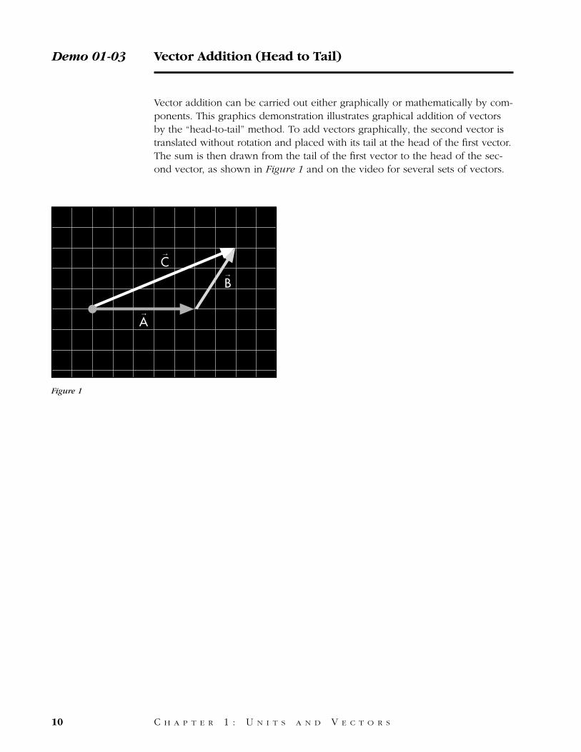
Vector addition can be carried out either graphically or mathematically by com-ponents. This graphics demonstration illustrates graphical addition of vectorsby the “head-to-tail” method. To add vectors graphically, the second vector istranslated without rotation and placed with its tail at the head of the first vector.The sum is then drawn from the tail of the first vector to the head of the sec-ond vector, as shown in Figure 1 and on the video for several sets of vectors.

Demo 01-03 Vector Addition (Head to Tail)


B→

A→

B→

C→

Figure 1

We’ll use these animated vector arrows to show a method of vector additioncalled head to tail addition. If we want to add vector B to vector A, we simplymove B so that its tail is in the same position as the head of A, keeping it par-allel to its original orientation at all times. The sum of the two vectors is foundby drawing a third vector from the tail of A to the head of B.

This is how the sum of the two vectors changes if vector B is rotated to dif-ferent orientations. Since the two vectors are equal in magnitude, their sumcan have a magnitude ranging from zero to twice that of A and B.

Vector Addition (Head to Tail) / Script Demo 01-03


Equipment

See Demonstration 01-02.

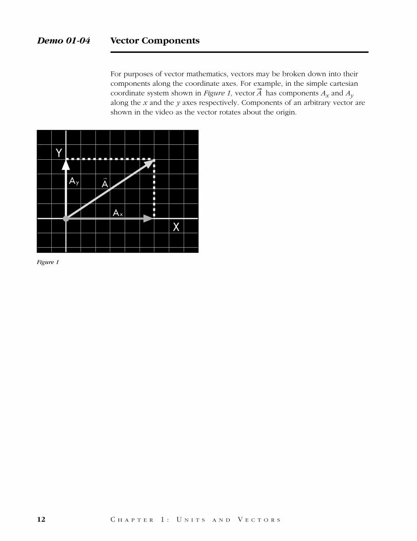
For purposes of vector mathematics, vectors may be broken down into theircomponents along the coordinate axes. For example, in the simple cartesiancoordinate system shown in Figure 1, vector

rA has components Ax and Ay

along the x and the y axes respectively. Components of an arbitrary vector areshown in the video as the vector rotates about the origin.

Demo 01-04 Vector Components


Y

X

Ay

Ax

A→

Figure 1

We’ll use this animated vector arrow to show how a vector can be brokendown into components, and how those components vary as the angle of thevector changes.

This vector can be broken down into two components, one along the x axis,and one along the y axis.

Here’s how the components change as the vector is rotated around the origin.

Vector Components / Script Demo 01-04


Equipment

See Demonstration 01-02.

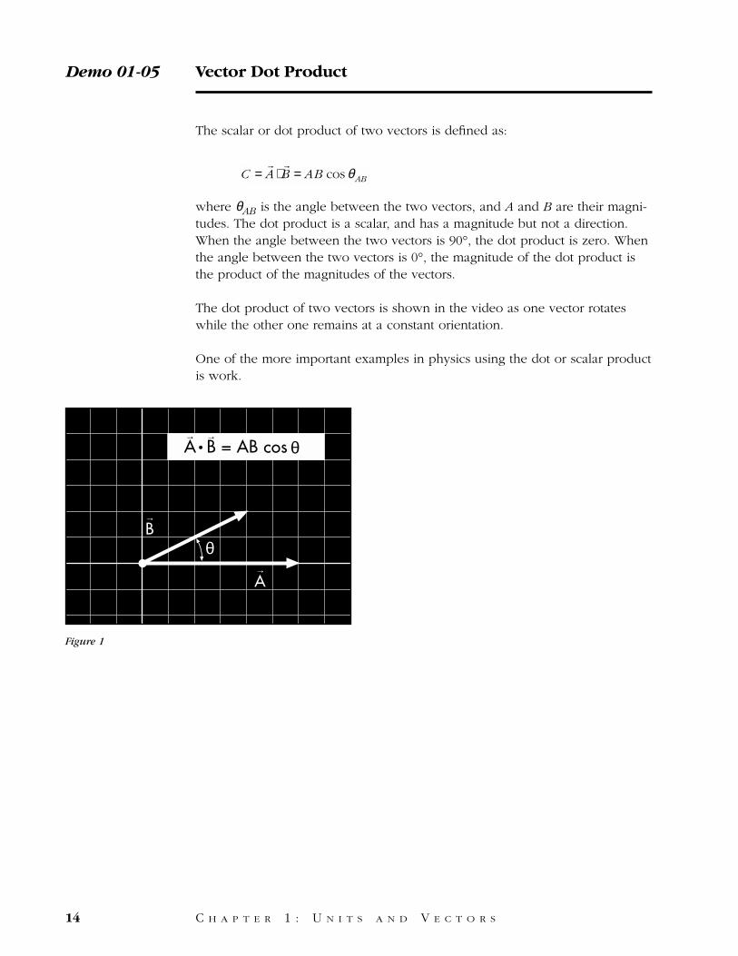
The scalar or dot product of two vectors is defined as:

where θAB is the angle between the two vectors, and A and B are their magni-tudes. The dot product is a scalar, and has a magnitude but not a direction.When the angle between the two vectors is 90°, the dot product is zero. Whenthe angle between the two vectors is 0°, the magnitude of the dot product isthe product of the magnitudes of the vectors.

The dot product of two vectors is shown in the video as one vector rotateswhile the other one remains at a constant orientation.

One of the more important examples in physics using the dot or scalar productis work.

C =rA ⋅

rB = AB cos θAB

Demo 01-05 Vector Dot Product


B→

θ

A B = AB cos θ•

A→

→ →

Figure 1

The dot product of two vectors is a scalar quantity which is equal to the prod-uct of their magnitudes times the cosine of the angle between them.

We’ll use these animated vectors to show how the dot product of two vectorsvaries as the angle between the vectors changes.

Vector Dot Product / Script Demo 01-05


Equipment

This demonstration is an animation.

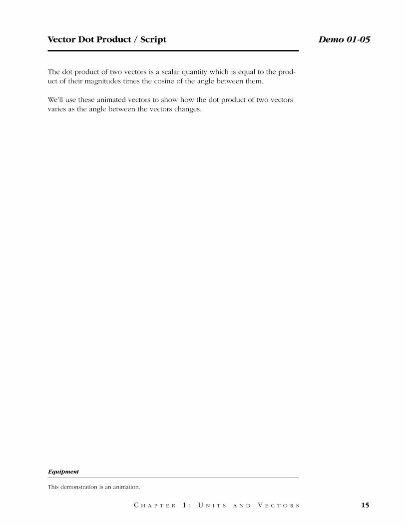
The vector or cross product of two vectors is defined as:

where θAB is the angle between the two vectors and A and B are their magni-tudes. Notice that

rC is a vector with the direction of the unit vector , per-

pendicular to the plane of A and B. The direction of the cross product can beobtained as follows: rotate a right-handed (standard) screw such that it rotatesfrom the vector

rA to the vector

rB through the smaller of the two angles be-

tween them. The screw will then drive in the direction of the cross productvector. Equivalently, if you curl the fingers of your right hand in the directionfrom

rA to

rB through the smaller of the angles between the vectors, your

thumb will point in the direction of the vector product.

Another variation of the right hand rule for vector cross product is illustrated inFigure 1: Using the fingers on your right hand, if the index finger points in thedirection of vector

rA and your middle finger points in the direction of vectorr

B , then the thumb will point in the direction of the cross product rC .

When the angle between the two vectors iseither 0° or 180°, the cross product is zero.When the angle between the two vectors is 90°,the magnitude of the cross product is the prod-uct of the magnitudes of the two vectors.

The cross product of two vectors is shown inthe video as one of the two vectors rotatesaround the origin while the other remains fixed.

Examples of the cross product in physicsinclude torque and the magnetic force on amoving charged particle.

c

rC =

rA×

rB = AB sinθAB

)c

Demo 01-06 Vector Cross Product


Figure 1

B→ B

→C = A + B→→

→

A→

A→

B→

We’ll use these animated vector arrows to show how the cross product of twovectors varies as the angle between them is changed.

The cross product of these two vectors, A and B, is a vector at right angles toboth. Its direction can be found using the right-hand rule.

The magnitude of a cross product of two vectors is equal to the product oftheir magnitudes times the sine of the angle between them.

Here’s how the cross product of A and B changes as the angle between themis changed.

Vector Cross Product / Script Demo 01-06


Equipment

This demonstration is an animation.

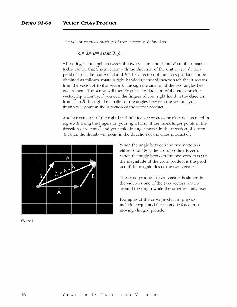
This demonstration extends the vector concept of Demonstration 01-04 tothree dimensions. The video shows several vectors in three dimensions on anx-y-z cartesian coordinate system of axes.

The orientation of the vector is now defined by three angles, the angles be-tween the vector and each of the three axes. Notice that the angle between thevector and any axis is not the same as the projection of that angle on any oneof the three planes containing two axes.

The apparatus used in the demonstration is shown in Figure 1, viewing alongthe x axis, so that the y and the z components are apparent.

Demo 01-07 3-D Vector Components


A→

X

Figure 1

This metal frame is a model of a three-dimensional coordinate system, with x,y, and z axes.

A vector that is anchored at the origin is free to move in the volume definedby the three axes.

We’ll move it to different positions in the frame and look at the model alongeach of the three axes to show the components of the vector on those axes.

When we look along the z axis, we see the components of the vector in the xand y axes.

Looking along the y axis shows the components along the x and z axes.

Looking along the x axis shows the components along the y and z axes.

Now we’ll change the position of the vector in the frame and repeat the se-quence.

3-D Vector Components / Script Demo 01-07


Equipment

A model vector coordinate system with a resultant vector that is free to move in space is usedfor this demonstration.

20

C H A P T E R 2

L I N E A R K I N E M A T I C S

21

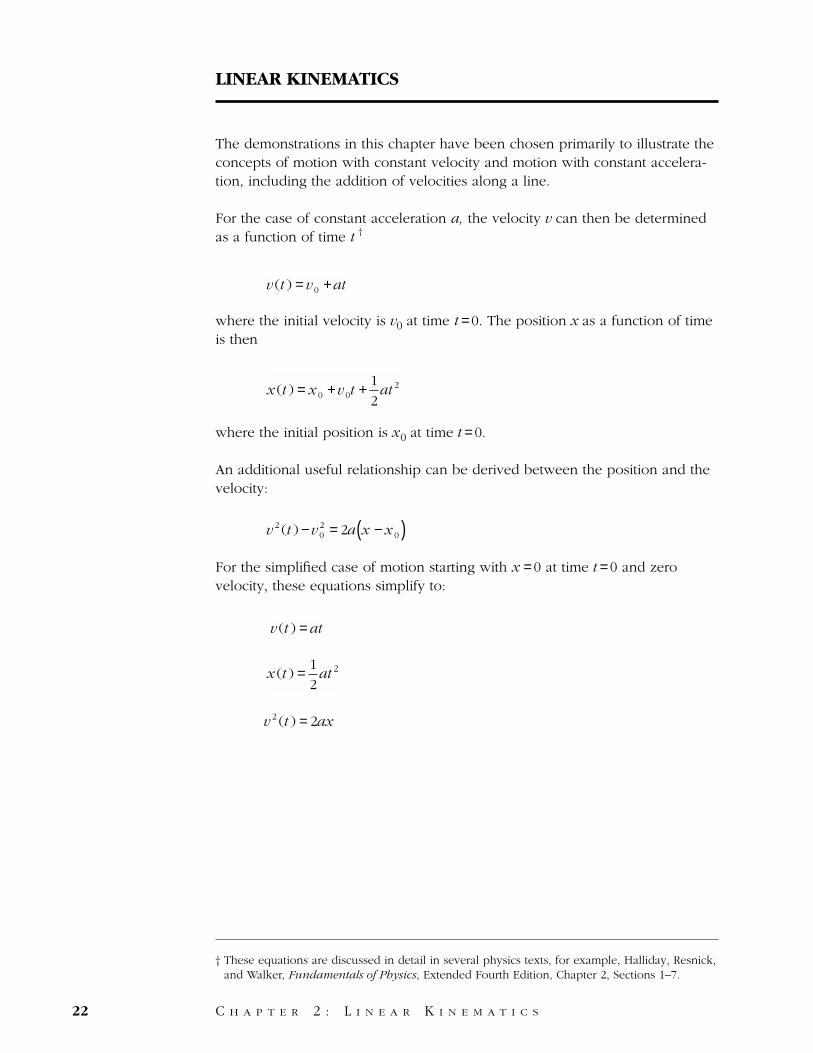
† These equations are discussed in detail in several physics texts, for example, Halliday, Resnick,and Walker, Fundamentals of Physics, Extended Fourth Edition, Chapter 2, Sections 1–7.

The demonstrations in this chapter have been chosen primarily to illustrate theconcepts of motion with constant velocity and motion with constant accelera-tion, including the addition of velocities along a line.

For the case of constant acceleration a, the velocity v can then be determinedas a function of time t †

where the initial velocity is v0 at time t =0. The position x as a function of timeis then

where the initial position is x0 at time t =0.

An additional useful relationship can be derived between the position and thevelocity:

For the simplified case of motion starting with x =0 at time t =0 and zerovelocity, these equations simplify to:

v2 (t ) = 2ax

x (t ) = 1

2at 2

v (t ) =at

v2 (t ) −v 0

2 = 2a x −x 0( )

x (t ) = x 0 +v 0t + 1

2at 2

v (t ) =v 0 +at

LINEAR KINEMATICS

22 C H A P T E R 2 : L I N E A R K I N E M A T I C S

23

This demonstration illustrates constant velocity using an air track glider. For thecase of constant velocity, the distance traveled by the glider in equal timeintervals is the same, which can be seen by marking the position of the glideron the video screen at a series of equal time intervals.

Each end of the air track is fitted with spring bouncers. This ensures that theglider collides elastically with the end of the air track, so that its speed is thesame but its direction is reversed, changing the velocity vector from +

rv to −

rv .

Demo 01-08 Constant Velocity


Figure 1

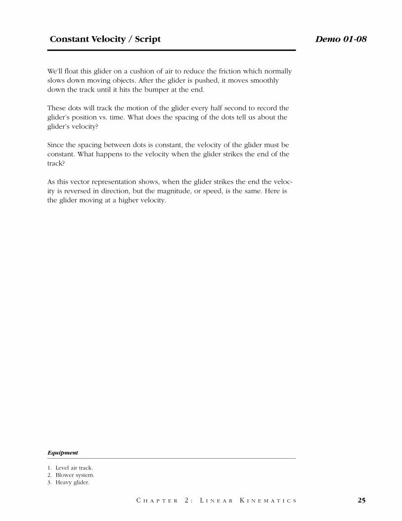
We’ll float this glider on a cushion of air to reduce the friction which normallyslows down moving objects. After the glider is pushed, it moves smoothlydown the track until it hits the bumper at the end.

These dots will track the motion of the glider every half second to record theglider’s position vs. time. What does the spacing of the dots tell us about theglider’s velocity?

Since the spacing between dots is constant, the velocity of the glider must beconstant. What happens to the velocity when the glider strikes the end of thetrack?

As this vector representation shows, when the glider strikes the end the veloc-ity is reversed in direction, but the magnitude, or speed, is the same. Here isthe glider moving at a higher velocity.

Constant Velocity / Script Demo 01-08

C H A P T E R 2 : L I N E A R K I N E M A T I C S 25

Equipment

1. Level air track.2. Blower system.3. Heavy glider.

This experiment demonstrates addition and subtraction of velocities along aline using two toy bulldozers and a paper sheet.† One bulldozer moves with aconstant velocity v1 over the table. The second bulldozer moves with the sameconstant velocity v1 on a paper sheet that can be moved along the same line asthe velocity of the bulldozer. This arrangement is shown in Figure 1.

If the paper sheet remains at rest, the two bulldozers move along together inthe same direction at velocities of v1. If the paper sheet is pulled with a ve-locity v2 in the same direction as the bulldozer, the velocity of the bulldozer inthe laboratory frame of reference will increase to v1+ v2. If the paper sheet ispulled with the same speed in the opposite direction, the velocity of the bull-dozer in the laboratory frame will decrease to v1− v2.

Demo 01-09 Bulldozer on Moving Sheet


† Freier and Anderson, A Demonstration Handbook for Physics, Demonstration Mb-30, RelativeVelocity.

Figure 1

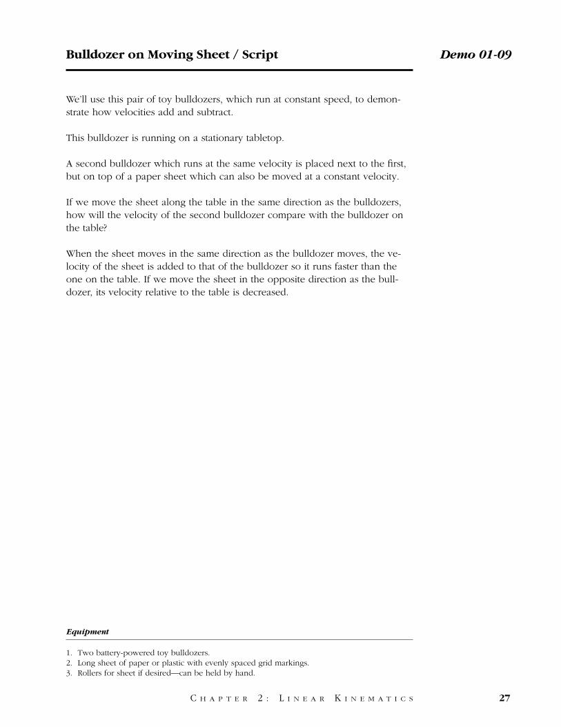
We’ll use this pair of toy bulldozers, which run at constant speed, to demon-strate how velocities add and subtract.

This bulldozer is running on a stationary tabletop.

A second bulldozer which runs at the same velocity is placed next to the first,but on top of a paper sheet which can also be moved at a constant velocity.

If we move the sheet along the table in the same direction as the bulldozers,how will the velocity of the second bulldozer compare with the bulldozer onthe table?

When the sheet moves in the same direction as the bulldozer moves, the ve-locity of the sheet is added to that of the bulldozer so it runs faster than theone on the table. If we move the sheet in the opposite direction as the bull-dozer, its velocity relative to the table is decreased.

Bulldozer on Moving Sheet / Script Demo 01-09


Equipment

1. Two battery-powered toy bulldozers.2. Long sheet of paper or plastic with evenly spaced grid markings.3. Rollers for sheet if desired—can be held by hand.

† Sutton, Demonstration Experiments in Physics, Demonstration M-77, Timed-interval InclinedPlane, page 39.

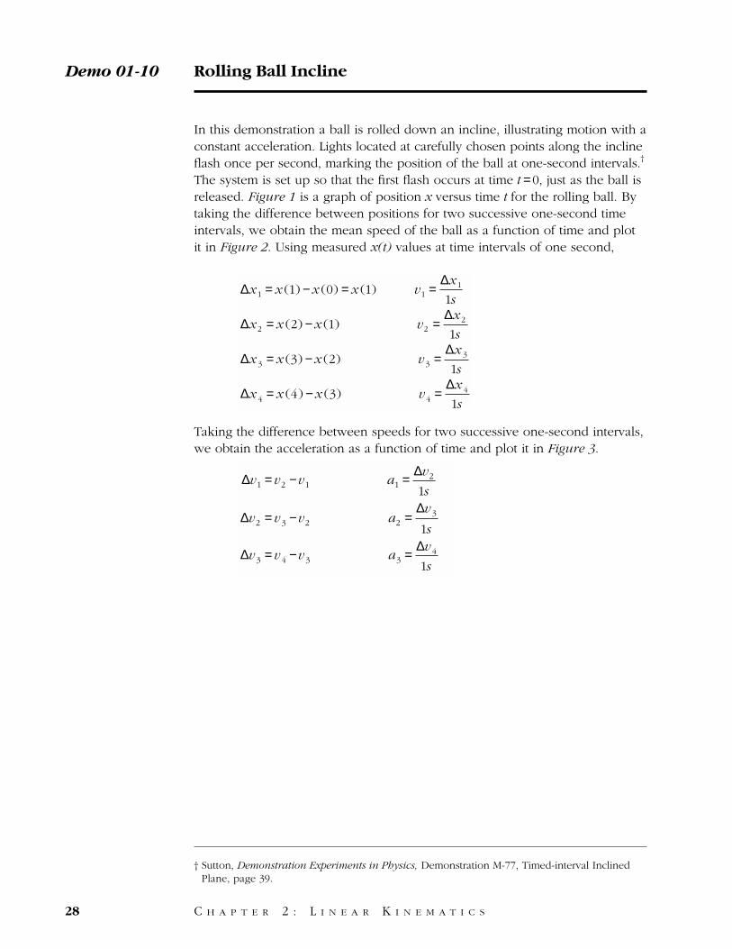
In this demonstration a ball is rolled down an incline, illustrating motion with aconstant acceleration. Lights located at carefully chosen points along the inclineflash once per second, marking the position of the ball at one-second intervals.†

The system is set up so that the first flash occurs at time t =0, just as the ball isreleased. Figure 1 is a graph of position x versus time t for the rolling ball. Bytaking the difference between positions for two successive one-second timeintervals, we obtain the mean speed of the ball as a function of time and plotit in Figure 2. Using measured x(t) values at time intervals of one second,

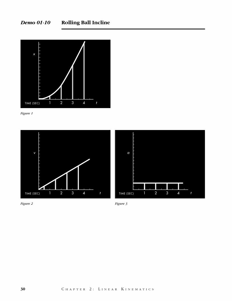
Taking the difference between speeds for two successive one-second intervals,we obtain the acceleration as a function of time and plot it in Figure 3.

∆v1 =v2 −v1 a1 =∆v2

1s

∆v2 =v 3 −v2 a2 =∆v 3

1s

∆v 3 =v 4 −v 3 a3 =∆v 4

1s

∆x1 = x (1) −x (0) = x (1) v1 =∆x1

1s

∆x2 = x (2) −x (1) v2 =∆x2

1s

∆x 3 = x (3) −x (2) v 3 =∆x 3

1s

∆x 4 = x (4) −x (3) v 4 =∆x 4

1s

Demo 01-10 Rolling Ball Incline


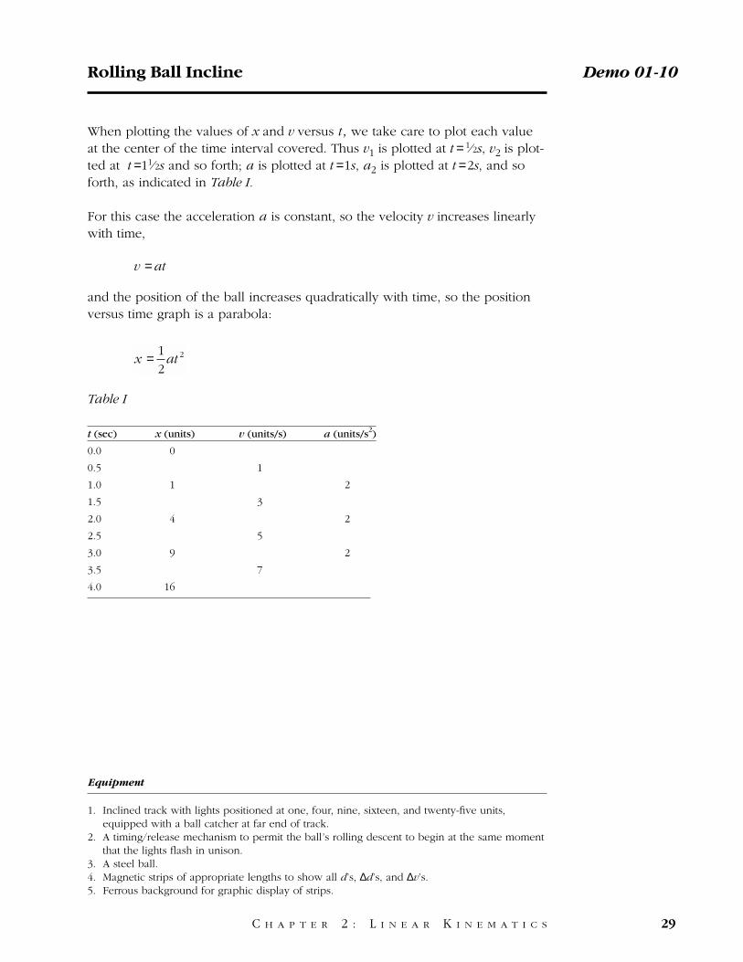
When plotting the values of x and v versus t , we take care to plot each valueat the center of the time interval covered. Thus v1 is plotted at t = 1⁄ 2s, v2 is plot-ted at t =11⁄ 2s and so forth; a is plotted at t =1s, a2 is plotted at t =2s, and soforth, as indicated in Table I.

For this case the acceleration a is constant, so the velocity v increases linearlywith time,

and the position of the ball increases quadratically with time, so the positionversus time graph is a parabola:

Table I

t (sec) x (units) v (units/s) a (units/s2)

0.0 0

0.5 1

1.0 1 2

1.5 3

2.0 4 2

2.5 5

3.0 9 2

3.5 7

4.0 16

x = 1

2at 2

v =at

Rolling Ball Incline Demo 01-10


Equipment

1. Inclined track with lights positioned at one, four, nine, sixteen, and twenty-five units,equipped with a ball catcher at far end of track.

2. A timing/release mechanism to permit the ball’s rolling descent to begin at the same momentthat the lights flash in unison.

3. A steel ball.4. Magnetic strips of appropriate lengths to show all d’s, ∆d’s, and ∆v’s.5. Ferrous background for graphic display of strips.

Demo 01-10 Rolling Ball Incline


TIME (SEC) 1 2 3 4 t

x

Figure 1


v

Figure 2


a

Figure 3

A ball rolling down a long incline will be used to show how position, velocity,and acceleration of the ball change as it moves down the incline.

Five lights arranged along the length of the track flash simultaneously once persecond.

As the ball rolls down it is directly above each of the lights just as they flash. Thisgives us a record of the positions of the ball at one-second intervals.

This is how far the ball traveled in the first second.

This is how far the ball traveled in the first two seconds.

Three seconds.

Four seconds.

We will move this distance up to a graph to keep track of position vs. time.

Does position change linearly over time?

Next we will graph the average velocity of the ball during five different inter-vals to see how velocity varies as the ball rolls down the incline. The ballmoved this far during the first second.

It moved this far during the next second.

This far during the third second.

The fourth second.

This gives us a graph of the velocity of the ball over time. Does velocity in-crease linearly?

Now we will graph the changes in velocity vs. time by graphing the differ-ences in successive velocities.

What does this tell us about the acceleration of the ball?

The acceleration is constant.

Rolling Ball Incline / Script Demo 01-10


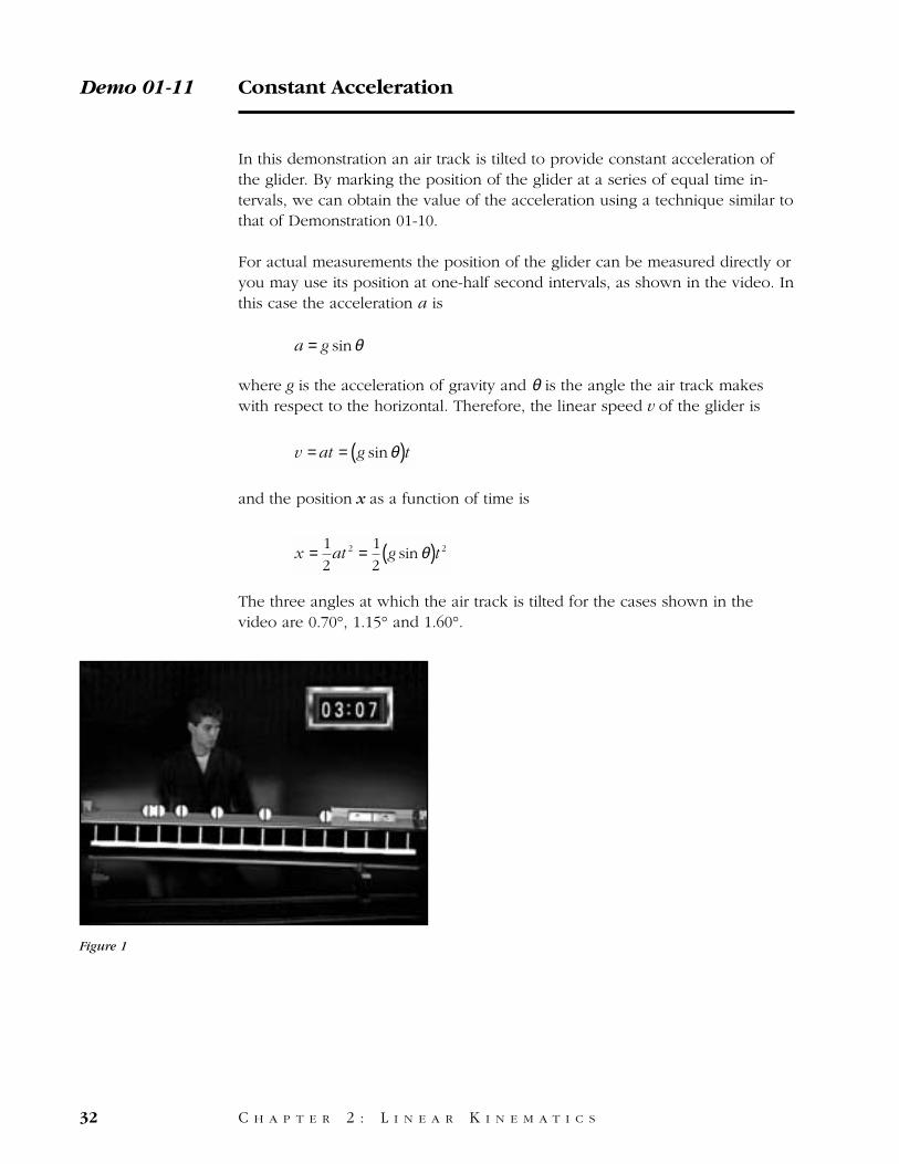
In this demonstration an air track is tilted to provide constant acceleration ofthe glider. By marking the position of the glider at a series of equal time in-tervals, we can obtain the value of the acceleration using a technique similar tothat of Demonstration 01-10.

For actual measurements the position of the glider can be measured directly oryou may use its position at one-half second intervals, as shown in the video. Inthis case the acceleration a is

where g is the acceleration of gravity and θ is the angle the air track makeswith respect to the horizontal. Therefore, the linear speed v of the glider is

and the position x as a function of time is

The three angles at which the air track is tilted for the cases shown in thevideo are 0.70°, 1.15° and 1.60°.

x = 1

2at 2 = 1

2g sin θ( )t 2

v =at = g sinθ( )t

a = g sinθ

Demo 01-11 Constant Acceleration


Figure 1

We will use a nearly frictionless air track with a glider floating on an air cush-ion to demonstrate accelerated motion.

When the track is level, a push is required to move the glider. It then moves ata constant velocity as shown by these dots that track the position of the gliderat half-second intervals.

When we tilt the track by placing a 1-centimeter high shim under one end, theglider moves down the track.

What can we say about the magnitude of the velocity in this case?

The glider’s velocity increases with time—it accelerates. If we increase the tiltof the track by doubling the height of the shim, the acceleration increases.

When the shim height is increased to 3 centimeters, the acceleration increasesagain.

This split-screen view shows the glider accelerating at all three angles of tilt.

Constant Acceleration / Script Demo 01-11


Equipment

1. Level air track.2. Blower system.3. Heavy glider.4. Multiple spacing shim to incline track.

† Sutton, Demonstration Experiments in Physics, Demonstration M-84, Freely Falling Bodies.Meiners, Physics Demonstration Experiments, Section 7-1.12, Freely Falling Bodies, page 113.Freier and Anderson, A Demonstration Handbook for Physics, Demonstration Mb-12, TimeIntervals of Fall.

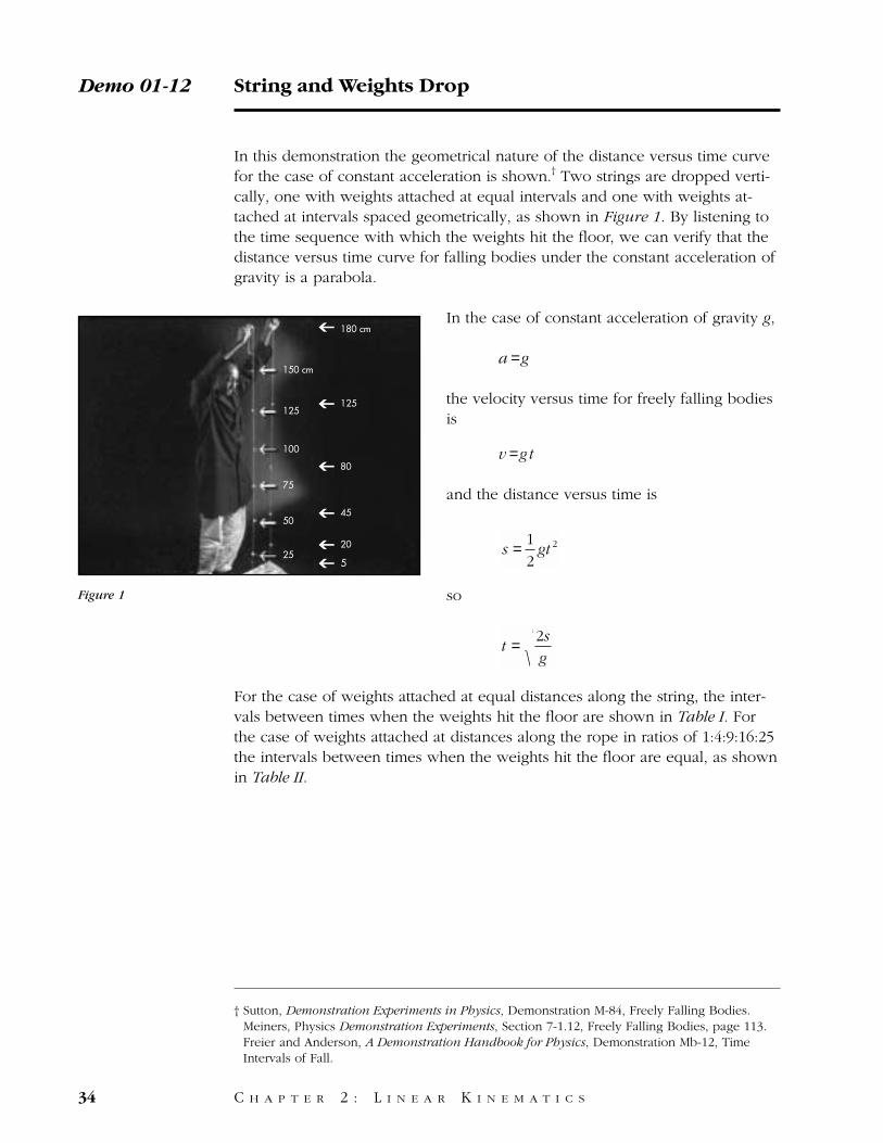
In this demonstration the geometrical nature of the distance versus time curvefor the case of constant acceleration is shown.† Two strings are dropped verti-cally, one with weights attached at equal intervals and one with weights at-tached at intervals spaced geometrically, as shown in Figure 1. By listening tothe time sequence with which the weights hit the floor, we can verify that thedistance versus time curve for falling bodies under the constant acceleration ofgravity is a parabola.

In the case of constant acceleration of gravity g,

a =g

the velocity versus time for freely falling bodiesis

v =gt

and the distance versus time is

so

For the case of weights attached at equal distances along the string, the inter-vals between times when the weights hit the floor are shown in Table I. Forthe case of weights attached at distances along the rope in ratios of 1:4:9:16:25the intervals between times when the weights hit the floor are equal, as shownin Table II.

t = 2s

g

s = 1

2gt 2

Demo 01-12 String and Weights Drop


➔

➔

➔

➔

➔

180 cm

125

80

45

20

5

➔

150 cm

100

75

50

25

125

Figure 1

Table I

s (cm) t (s) ∆t (s)

0 0.000

25 0.226 0.226

50 0.319 0.093

75 0.391 0.072

100 0.452 0.061

125 0.505 0.053

150 0.553 0.048

String and Weights Drop Demo 01-12

String and Weights Drop / Script Demo 01-12


Table II

s (cm) t (s) ∆t (s)

0 0.000

5 0.101 0.101

20 0.202 0.101

45 0.303 0.101

80 0.404 0.101

125 0.505 0.101

180 0.606 0.101

On the left is a string with small weights tied at regular increasing heightsabove the ground. We’ll drop the string and listen to the sound as each weightstrikes a board at the bottom.

When the string is dropped, the weights strike the board in decreasing inter-vals of time.

On this string, the height of the weights increases geometrically.

When this string is dropped, the weights strike the board at equal intervals oftime.

Equipment

1. A string tied with equally spaced weights.2. A string tied with weights with geometrically increasing spacing.3. A board on which one can drop the two series of weights and utilize the emitted sound to

judge the time intervals of the weights striking the board.

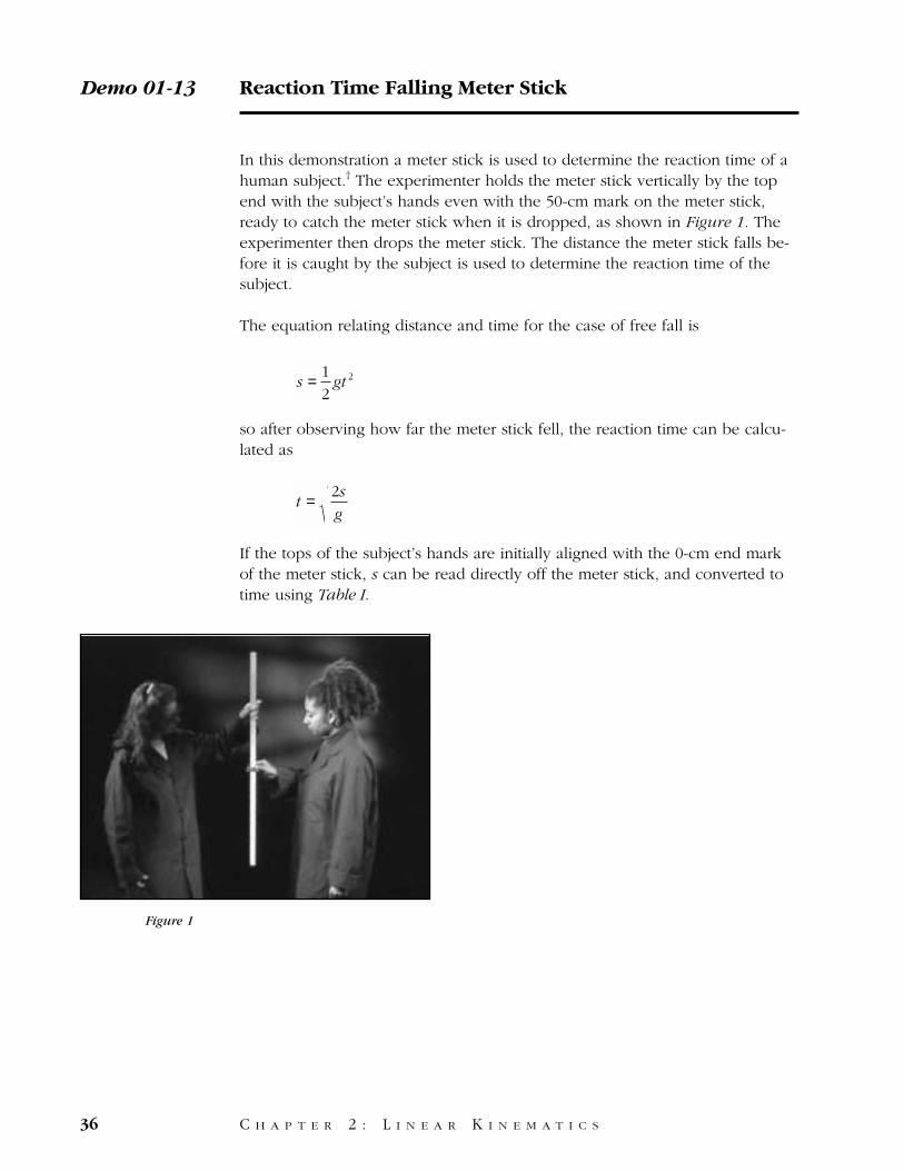
In this demonstration a meter stick is used to determine the reaction time of ahuman subject.† The experimenter holds the meter stick vertically by the topend with the subject’s hands even with the 50-cm mark on the meter stick,ready to catch the meter stick when it is dropped, as shown in Figure 1. Theexperimenter then drops the meter stick. The distance the meter stick falls be-fore it is caught by the subject is used to determine the reaction time of thesubject.

The equation relating distance and time for the case of free fall is

so after observing how far the meter stick fell, the reaction time can be calcu-lated as

If the tops of the subject’s hands are initially aligned with the 0-cm end markof the meter stick, s can be read directly off the meter stick, and converted totime using Table I.

t = 2s

g

s = 1

2gt 2

Demo 01-13 Reaction Time Falling Meter Stick


Figure 1

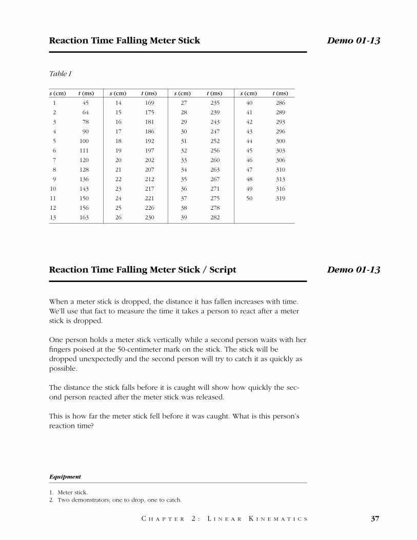
Table I

s (cm) t (ms) s (cm) t (ms) s (cm) t (ms) s (cm) t (ms)

1 45 14 169 27 235 40 286

2 64 15 175 28 239 41 289

3 78 16 181 29 243 42 293

4 90 17 186 30 247 43 296

5 100 18 192 31 252 44 300

6 111 19 197 32 256 45 303

7 120 20 202 33 260 46 306

8 128 21 207 34 263 47 310

9 136 22 212 35 267 48 313

10 143 23 217 36 271 49 316

11 150 24 221 37 275 50 319

12 156 25 226 38 278

13 163 26 230 39 282

Reaction Time Falling Meter Stick Demo 01-13


Reaction Time Falling Meter Stick / Script Demo 01-13

When a meter stick is dropped, the distance it has fallen increases with time.We’ll use that fact to measure the time it takes a person to react after a meterstick is dropped.

One person holds a meter stick vertically while a second person waits with herfingers poised at the 50-centimeter mark on the stick. The stick will bedropped unexpectedly and the second person will try to catch it as quickly aspossible.

The distance the stick falls before it is caught will show how quickly the sec-ond person reacted after the meter stick was released.

This is how far the meter stick fell before it was caught. What is this person’sreaction time?

Equipment

1. Meter stick.2. Two demonstrators; one to drop, one to catch.

† Sutton, Demonstration Experiments in Physics, Demonstration M-79, Guinea-and-Feather Tube.

This is the classic demonstration showing that the acceleration of free fall isindependent of mass, in the absence of other significant forces such as air fric-tion.† A metal disc and a small piece of paper are placed inside two identicalvertical glass tubes, and the tubes are rapidly rotated so the objects remainstuck at one end. When the tubes are upside down, the disc and the paperbegin to fall to the lower end. Due to air drag the paper falls more slowly thanthe disc. When the air is pumped out of the tube, the disc and the paper fallwith the same acceleration and reach the bottom end of the tube at the sametime.

Demo 01-14 Guinea and Feather


Figure 1

We are used to seeing light objects fall more slowly than heavy objects. Butwhy do light and heavy objects fall differently?

We will use this pair of tubes containing metal and paper discs to show theeffect of eliminating air resistance. This is how the objects fall when the tubesare filled with air.

If we now remove most of the air from the tubes with a vacuum pump andrepeat the demonstration, the results change dramatically.

Guinea and Feather / Script Demo 01-14


Equipment

1. Guinea and feather tube—sealed and equipped for evacuation.2. Vacuum pump.3. Perhaps a light and heavier object to drop through open atmosphere as a comparison.

40

C H A P T E R 3

L I N E A R D Y N A M I C S

4141

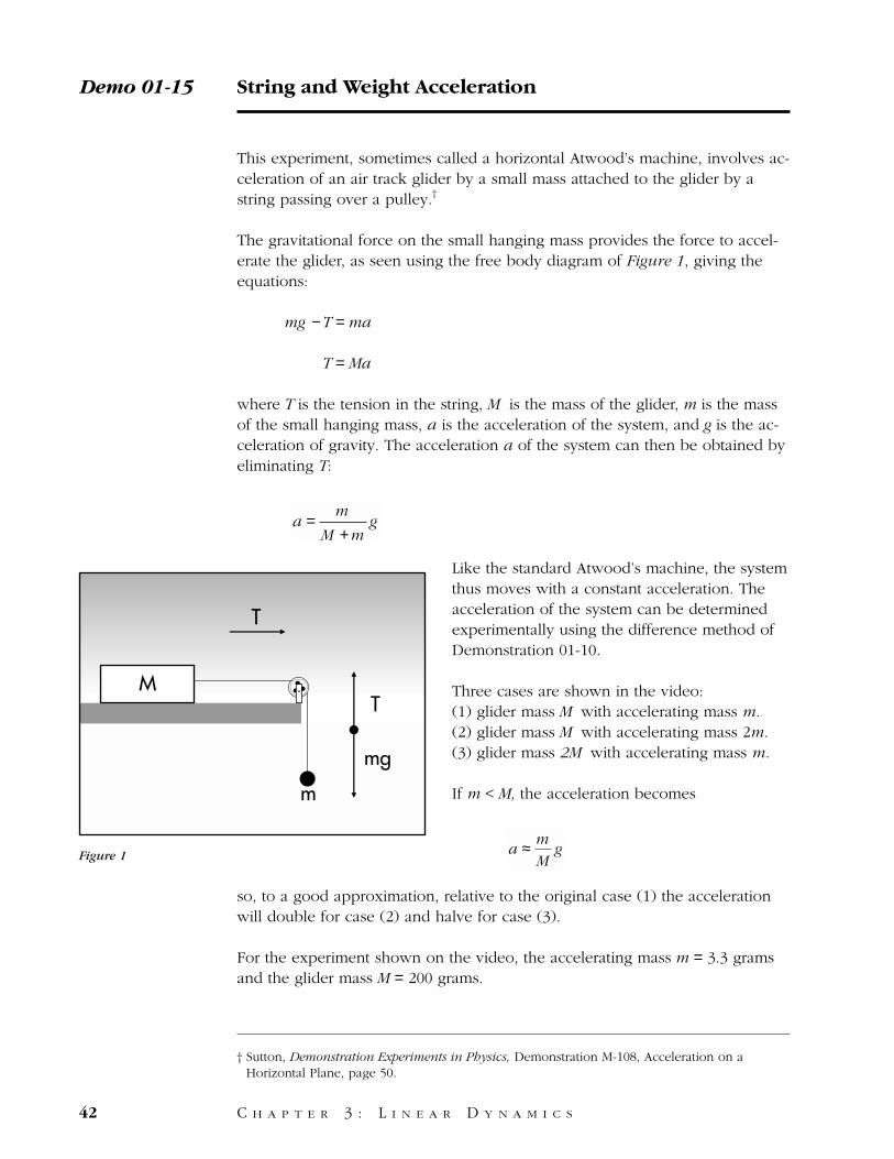
This experiment, sometimes called a horizontal Atwood’s machine, involves ac-celeration of an air track glider by a small mass attached to the glider by astring passing over a pulley.†

The gravitational force on the small hanging mass provides the force to accel-erate the glider, as seen using the free body diagram of Figure 1, giving theequations:

mg −T = ma

T = Ma

where T is the tension in the string, M is the mass of the glider, m is the massof the small hanging mass, a is the acceleration of the system, and g is the ac-celeration of gravity. The acceleration a of the system can then be obtained byeliminating T:

Like the standard Atwood’s machine, the systemthus moves with a constant acceleration. Theacceleration of the system can be determinedexperimentally using the difference method ofDemonstration 01-10.

Three cases are shown in the video: (1) glider mass M with accelerating mass m.(2) glider mass M with accelerating mass 2m.(3) glider mass 2M with accelerating mass m.

If m < M, the acceleration becomes

so, to a good approximation, relative to the original case (1) the accelerationwill double for case (2) and halve for case (3).

For the experiment shown on the video, the accelerating mass m = 3.3 gramsand the glider mass M = 200 grams.

a ≈ m

Mg

a =m

M +mg

Demo 01-15 String and Weight Acceleration

42 C H A P T E R 3 : L I N E A R D Y N A M I C S

MT

mg

m

T

Figure 1

† Sutton, Demonstration Experiments in Physics, Demonstration M-108, Acceleration on aHorizontal Plane, page 50.

If a string hanging over a pulley is loaded with a small weight, it provides aforce which can accelerate a glider floating on a cushion of air.

Here is the same acceleration, with the position of the glider marked by dots athalf-second intervals.

If the force is doubled by doubling the hanging mass, how will that affect theacceleration of the glider?

The dots are more widely spaced, so the acceleration has increased.

If the same hanging weight is now used but the glider’s mass is doubled, howwill the acceleration change?

Here is the new acceleration.

Here are all three accelerations and the force and mass data for each.

String and Weight Acceleration / Script Demo 01-15

C H A P T E R 3 : L I N E A R D Y N A M I C S 43

Equipment

1. Level air track. 2. Blower system.3. Glider.4. Two low-friction pulleys.5. Very lightweight length of string. 6. A supply of paper clips.7. Support system for pulleys.8. Appropriate masses to double the glider’s weight.9. Perhaps a stopwatch to measure the time of fall.

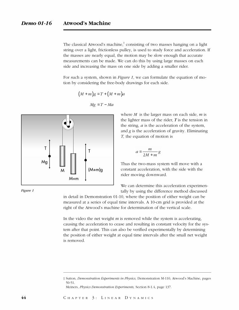
The classical Atwood’s machine,† consisting of two masses hanging on a lightstring over a light, frictionless pulley, is used to study force and acceleration. Ifthe masses are nearly equal, the motion may be slow enough that accuratemeasurements can be made. We can do this by using large masses on eachside and increasing the mass on one side by adding a smaller rider.

For such a system, shown in Figure 1, we can formulate the equation of mo-tion by considering the free-body drawings for each side.

where M is the larger mass on each side, m isthe lighter mass of the rider, T is the tension inthe string, a is the acceleration of the system,and g is the acceleration of gravity. EliminatingT, the equation of motion is

Thus the two-mass system will move with aconstant acceleration, with the side with therider moving downward.

We can determine this acceleration experimen-tally by using the difference method discussed

in detail in Demonstration 01-10, where the position of either weight can bemeasured at a series of equal time intervals. A 10-cm grid is provided at theright of the Atwood’s machine for determination of the vertical scale.

In the video the net weight m is removed while the system is accelerating,causing the acceleration to cease and resulting in constant velocity for the sys-tem after that point. This can also be verified experimentally by determiningthe position of either weight at equal time intervals after the small net weightis removed.

a = m

2M +mg

Mg =T − Ma

M +m( )g =T + M +m( )a

Demo 01-16 Atwood’s Machine


Mg

(M+m)gM

M+m

TT

Figure 1

† Sutton, Demonstration Experiments in Physics, Demonstration M-110, Atwood’s Machine, pages50-51.Meiners, Physics Demonstration Experiments, Section 8-1.4, page 137.

This device is known as an Atwood’s machine.

Two equal masses hang on either side of a string passing over a pulley. Sincethe masses are equal, there is no net force to accelerate the masses and theyare in equilibrium in any position.

A small rider is now added to one of the large masses, and the system beginsto move.

How could we best describe this type of motion?

Since there is a constant unbalanced force on the system, it is accelerated.

The traces left behind each half-second in this segment show the acceleration.

If the mass now passes through this ring so that the rider is picked off, howwill the motion of the masses be affected?

The masses now move with a constant velocity.

Here is the same sequence repeated with two riders added to the large mass.

Atwood’s Machine / Script Demo 01-16


Equipment

1. A very low-friction pulley.2. Lightweight length of string. 3. Two masses of equal weight. 4. Two relatively small rider weights to take the system out of static balance.5. A catch system for the riders so that they are lifted off without disturbing the linear

downward motion.6. A stopwatch/clock.7. A two-meter stick.

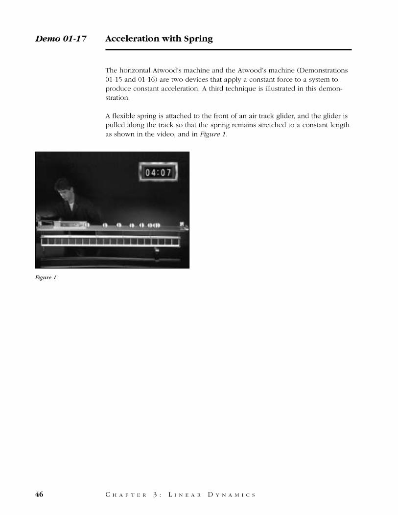
The horizontal Atwood’s machine and the Atwood’s machine (Demonstrations01-15 and 01-16) are two devices that apply a constant force to a system toproduce constant acceleration. A third technique is illustrated in this demon-stration.

A flexible spring is attached to the front of an air track glider, and the glider ispulled along the track so that the spring remains stretched to a constant lengthas shown in the video, and in Figure 1.

Demo 01-17 Acceleration with Spring


Figure 1

We will use a glider floating on a cushion of air and a light spring to demon-strate how a constant force from a spring can accelerate the glider.

The spring is attached to the end of the glider, and a marker stick is attachedto the top of the glider to indicate the extension of the spring.

When the spring is pulled out, it pulls on the glider with a constant force. Theforce from the spring accelerates the glider. Here is the same acceleration re-peated, with dots on the screen recording the position of the glider every halfsecond.

Acceleration with Spring / Script Demo 01-17


Equipment

1. Level air track. 2. Blower system.3. Heavy glider with extended marker bar.4. Two low-friction pulleys.5. Very lightweight spring with a small spring constant.

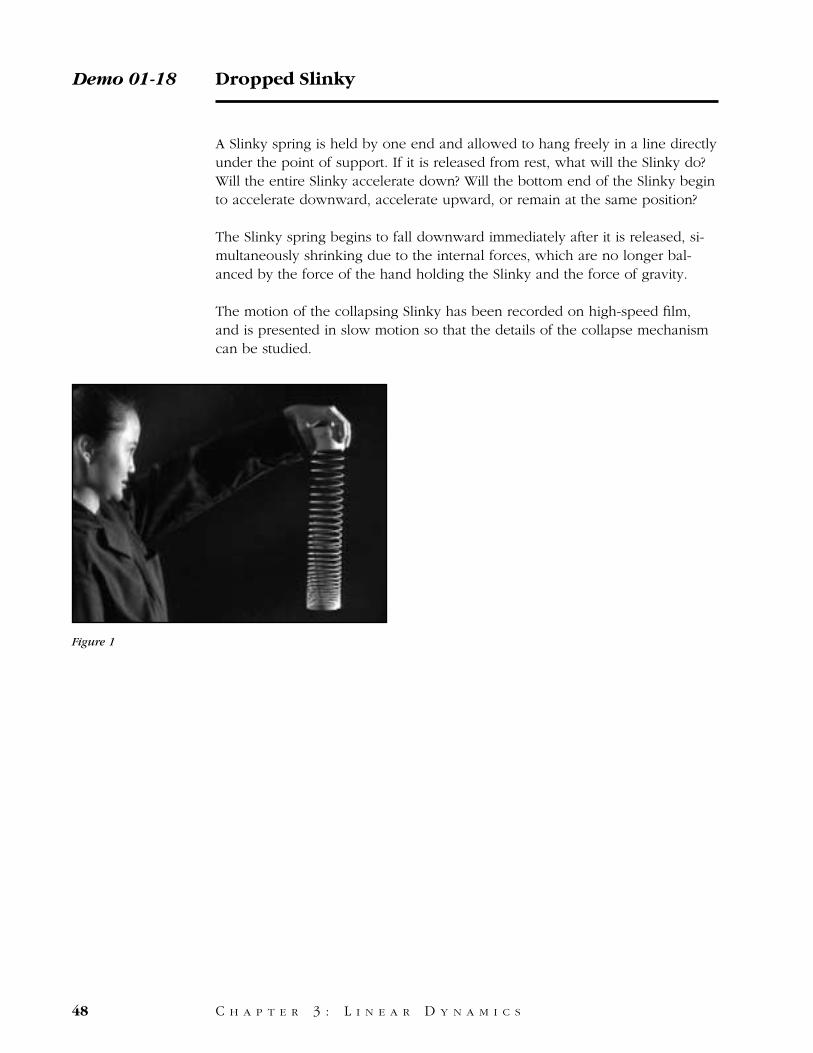
A Slinky spring is held by one end and allowed to hang freely in a line directlyunder the point of support. If it is released from rest, what will the Slinky do?Will the entire Slinky accelerate down? Will the bottom end of the Slinky beginto accelerate downward, accelerate upward, or remain at the same position?

The Slinky spring begins to fall downward immediately after it is released, si-multaneously shrinking due to the internal forces, which are no longer bal-anced by the force of the hand holding the Slinky and the force of gravity.

The motion of the collapsing Slinky has been recorded on high-speed film,and is presented in slow motion so that the details of the collapse mechanismcan be studied.

Demo 01-18 Dropped Slinky


Figure 1

When this spring is held at the top and allowed to hang, the weight of thespring stretches it out. If we release the spring, its weight will still be pullingon it during the fall. What will happen to the length of the spring during thefall?

The spring immediately contracts when it is dropped.

Dropped Slinky / Script Demo 01-18


Equipment

One Slinky.

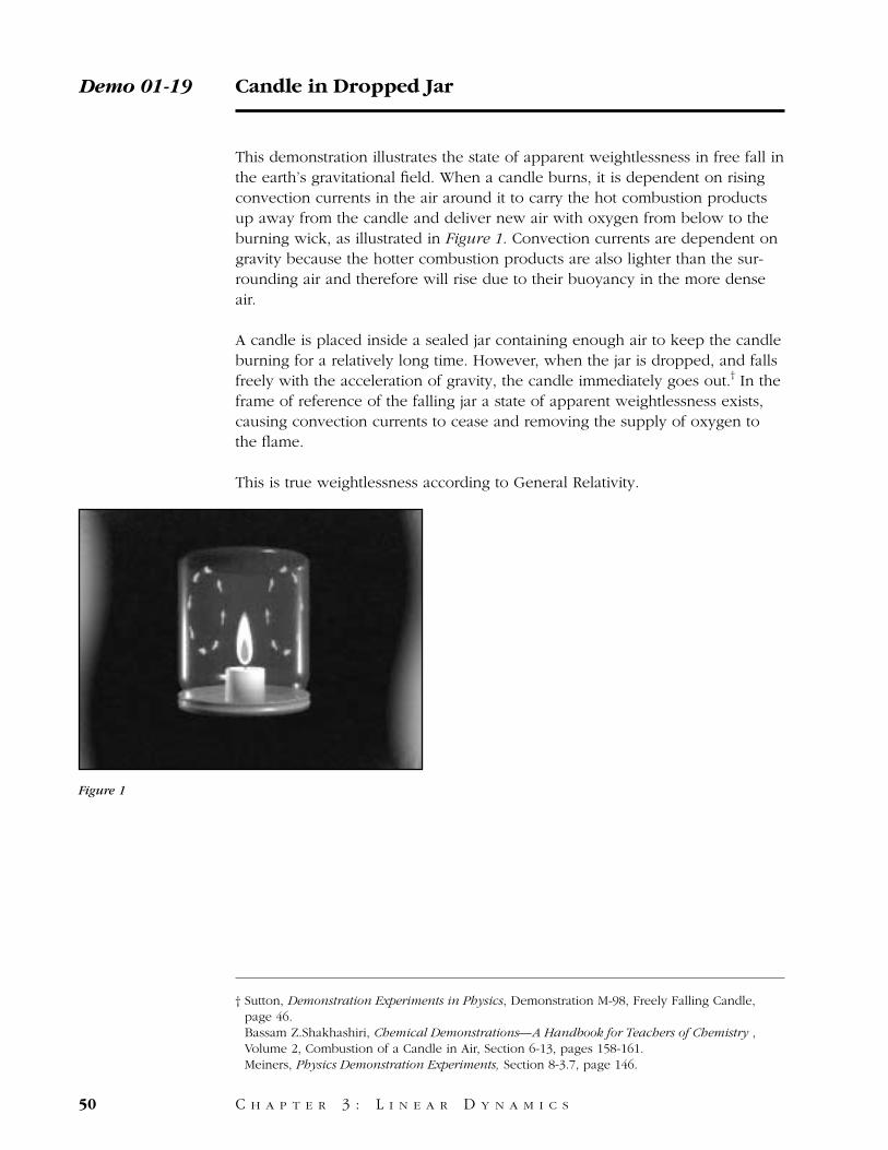
This demonstration illustrates the state of apparent weightlessness in free fall inthe earth’s gravitational field. When a candle burns, it is dependent on risingconvection currents in the air around it to carry the hot combustion productsup away from the candle and deliver new air with oxygen from below to theburning wick, as illustrated in Figure 1. Convection currents are dependent ongravity because the hotter combustion products are also lighter than the sur-rounding air and therefore will rise due to their buoyancy in the more denseair.

A candle is placed inside a sealed jar containing enough air to keep the candleburning for a relatively long time. However, when the jar is dropped, and fallsfreely with the acceleration of gravity, the candle immediately goes out.† In theframe of reference of the falling jar a state of apparent weightlessness exists,causing convection currents to cease and removing the supply of oxygen tothe flame.

This is true weightlessness according to General Relativity.

Demo 01-19 Candle in Dropped Jar


Figure 1

† Sutton, Demonstration Experiments in Physics, Demonstration M-98, Freely Falling Candle,page 46.Bassam Z.Shakhashiri, Chemical Demonstrations—A Handbook for Teachers of Chemistry ,Volume 2, Combustion of a Candle in Air, Section 6-13, pages 158-161. Meiners, Physics Demonstration Experiments, Section 8-3.7, page 146.

If we light a candle and place it inside a glass jar, there is enough oxygen inthe jar to let the candle burn for over 10 seconds.

Moving the jar rapidly from side to side does not have a great effect on theflame because the jar protects the flame from the wind caused by the motion.But what will happen if we relight the candle and drop the jar from a height often feet?

The flame goes out on the way down. When the jar is in free fall, there are noconvection currents to bring fresh oxygen up into the flame.

Candle in Dropped Jar / Script Demo 01-19


Equipment

1. Quart jar.2. Candle affixed to inside surface of jar’s lid.3. Source of flame.4. Catching device to protect glass jar.

Richard Manliffe Sutton, Demonstration Experiments in Physics (McGraw-Hill, NewYork,1938) out of print, but reprinted with permission by Kinko’s Copies, 114W.Franklin St., Chapel Hill, NC 27516.

Harry F. Meiners, Physics Demonstration Experiments, Volumes I and II (Ronald Press,New York, 1970).

G. D. Freier and F. J. Anderson, A Demonstration Handbook for Physicss (AmericanAssociation of Physics Teachers, College Park, MD, 1981).

Bassam Z.Shakhashiri, Chemical Demonstrations—A Handbook for Teachers of Chem-istry , Voilumes I and II (The University of Wisconsin Press, Madison, 1958).

Herbert L. Anderson, Editor-in-Chief, A Physicist’s Desk Reference, The Second Editionof Physics Vade Mecum (American Institute of Physics, New York, 1989), page 5.

Bibliography

52

Documents

The Video Encyclopedia of Physics Demonstrationsjedlik.phy.bme.hu/f29/dvd/01_brochure.pdf · 2005. 5. 3. · Physics Vade Mecum (American Institute of Physics, New York, 1989),