Embed Size (px)
Citation preview
This is a repository copy of The value of fault analysis for field development planning.
White Rose Research Online URL for this paper:http://eprints.whiterose.ac.uk/106864/
Version: Accepted Version
Article:
Frischbutter, AA, Fisher, QJ orcid.org/0000-0002-2881-7018, Namazova, G et al. (1 more author) (2017) The value of fault analysis for field development planning. Petroleum Geoscience, 23 (1). pp. 120-133. ISSN 1354-0793
https://doi.org/10.1144/petgeo2016-053
© 2016 The Author(s). Published by The Geological Society of London for GSL and EAGE.This is an author produced version of a paper published in Petroleum Geoscience 23(1):120-133 Feb 2017; https://doi.org/10.1144/petgeo2016-053. Uploaded in accordancewith the publisher's self-archiving policy.
[email protected]://eprints.whiterose.ac.uk/
Reuse
Unless indicated otherwise, fulltext items are protected by copyright with all rights reserved. The copyright exception in section 29 of the Copyright, Designs and Patents Act 1988 allows the making of a single copy solely for the purpose of non-commercial research or private study within the limits of fair dealing. The publisher or other rights-holder may allow further reproduction and re-use of this version - refer to the White Rose Research Online record for this item. Where records identify the publisher as the copyright holder, users can verify any specific terms of use on the publisher’s website.
Takedown
If you consider content in White Rose Research Online to be in breach of UK law, please notify us by emailing [email protected] including the URL of the record and the reason for the withdrawal request.

The value of fault analysis for field development planning 1
Andreas A. Frischbutter1*, Quentin J. Fisher2, Gyunay Namazova1 & Sebastien Dufour1 2
3
1Wintershall Norge AS, Laberget 28, 4020 Stavanger, Norway 4 2School of Earth and Environment, University of Leeds, Leeds, LS2 9JT, UK 5
*Corresponding author ([email protected]) 6
7
Work carried out at Wintershall Norge AS and Center for Integrated Petroleum Geoscience, 8
University of Leeds 9
10
Abbreviated title: Fault analysis in field development planning 11
12
Abstract: Faults play an important role in reservoir compartmentalization and can have a significant impact 13
on recoverable volumes. A recent petroleum discovery in the Norwegian offshore sector, with an Upper 14
Jurassic reservoir, is currently in the development planning phase. The reservoir is divided into several 15
compartments by syn-depositional faults that have not been reactivated and do not offset the petroleum-16
bearing sandstones completely. A comprehensive fault analysis has been conducted from core to seismic 17
scale to assess the likely influence of faults on the production performance and recoverable volumes. The 18
permeability of the small-scale faults from the core were analyzed at high confining pressures using 19
formation compatible brines. These permeability measurements provide important calibration points for the 20
fault property assessment, which was used to calculate transmissibility multipliers (TM) that were 21
incorporated into the dynamic reservoir simulation model to account for the impact of faults on fluid flow. 22
Dynamic simulation results reveal a range of more than 20% for recoverable volumes depending on the 23
fault property case applied and for a base case producer/injector well pattern. The fault properties are one 24
of the key parameters that influence the range of cumulative recoverable oil volumes and the recovery 25
efficiency. 26
27
Keywords: fault property analysis, fault permeability prediction, fault rock petrophysics, transmissibility 28
multiplier, dynamic reservoir simulation, field development planning 29
30
Introduction 31
A recently discovered oil field with a gas cap in the Norwegian offshore sector is currently in the 32
development planning phase. Four exploration/appraisal wells have been drilled in the field, but no 33
production data exists at this stage of the field lifecycle. Key uncertainties that impact recoverable volumes 34
and production behaviour range from reservoir distribution (i.e. sedimentologically-controlled 35
compartmentalization), reservoir properties, fault architecture and fault rock properties. In terms of the 36
latter, the field is compartmentalized by numerous faults at the seismic scale, but also contains numerous 37
sub-seismic scale faults. An understanding of the fault properties and their influence on the field production 38
and recoverable volumes is essential for assessing the fields economics, planning a production strategy and 39
also influences the design of the facilities. In this paper we focus on the impact of structural pattern and 40
fault rock properties on the subsurface fluid flow and hence the production. 41
Workflows exist for the quantitative assessment of the impact of faults on fluid flow in petroleum 42
reservoirs and can be implemented using a range of software tools that are commonly available (see review 43
by Fisher & Jolley, 2007). In general, the workflow begins by undertaking a structural analysis using 44
seismic data. Faults identified from seismic are then incorporated into the geological model. The clay 45
distribution along the faults is then estimated using well established algorithms. In siliciclastic reservoirs, 46
the main fault seal processes are: (i) cataclasis; (ii) mixing of clays with framework grains, (iii) clay smear, 47
and (iv) post-deformation diagenesis such as quartz cementation and grain-contact quartz dissolution 48
(Fisher and Knipe, 1998; 2001). The presence of clay is important for two of these mechanisms which often 49
results in correlations between fault permeability and clay content; these correlations may then be used to 50
calculate transmissibility multipliers (TM) that are incorporated into simulation models to take into account 51
the impact of faults on fluid flow. Fault rock permeability data can be obtained from global datasets. 52
However, some studies suggest that better results are obtained if fault permeability estimates are based on 53
the laboratory measurements made on fault rocks sampled from cores taken within the field being appraised 54
or from nearby analogues (Fisher & Knipe, 2001; Sperrevik et al., 2002; Jolley et al., 2007). 55
The study reported in this paper follows the general workflow described above. A key difference, however, 56
is that many fault compartmentalization studies use fault rock property data that was collected under 57
inappropriate laboratory conditions. For example, many studies use fault rock permeability data collected 58
at ambient confining pressures using brine compositions that are not compatible with the formation despite 59
a wealth of evidence to suggest that the permeability of tight rocks is very sensitive to the stress conditions 60
(e.g. Thomas and Ward, 1972) and the brine chemistry (e.g. Lever and Dawe, 1987). The current study 61
differs in that fault rock permeability measurements were made at high stresses using formation compatible 62

brines. The new fault rock permeability data has then been incorporated into the dynamic reservoir 63
simulation model to improve production forecasts. 64
65
Reservoir 66
The main reservoir is in Late Jurassic sandstones of the Heather Formation. The reservoir is 67
comprised of turbiditic sandstones, deposited syntectonically, during the main rifting event in the 68
Late Jurassic. The reservoir is currently located at a depth between 2400m – 2800m, with the 69
temperature at reservoir level being slightly above 90o C. Glacial melting during Pleistocene 70
times resulted in an uplift of approximately 300m. The reservoir thickness varies between 10m 71
and 130m (mean 60m). The N/G of the reservoir section varies between 55% and 73%. The 72
reservoir permeabilities range from 0.1 – 5 Darcy and porosities vary between 10% and 30%. 73
The reservoir experienced the precipitation of early K-feldspar overgrowths and kaolin during 74
shallow burial. Mechanical compaction was the main process for reducing porosity and 75
permeability during intermediate burial. The sandstones experienced small amounts of quartz 76
precipitation and grain contact quartz dissolution during deep burial. 77
78
Structural setting 79
The field is compartmentalized by numerous seismic scale, mainly NW-SE and NE-SW striking, normal 80
faults (Fig. 1a). East-West striking faults are present, but to a minor amount. The maximum fault throw 81
observed is around 60m with a mean around the seismic resolution of 25m. The main reservoir is self-82
juxtaposed throughout the field (Fig. 1b), implying that the properties of the fault rocks need to be 83
considered to predict the impact of faults on fluid flow during production. It is important to note that no 84
evidence of a static fault seal over geological time exists within the main part of the field. The wells drilled 85
in the main part of the field, e.g. well A, B, D, have pressures on a common gradient, which is consistent 86
with communication through the hydrocarbon phase. However, this cannot be taken as evidence that the 87
faults will not impact flow on a production time-scale. The hydrocarbon water contact has been drilled in 88
well B, whereas the wells A and D have an oil- and gas-down-to. 89
Deposition of the reservoir happened syntectonically and the turbidites were deposited in half grabens (Figs 90
2, 3). Faulting started in the Late Triassic and continued throughout the Early and Middle Jurassic, with the 91
main rifting in the Late Jurassic. In general, the tectonic activity ceased in the Latest Jurassic, but some 92
faults are active in the Early Cretaceous (Fig. 2). Structural restoration indicates that the faulting that 93
affected the reservoir occurred at relatively shallow depths (<1000m). 94
The main fault network only represents faults that could be mapped over a larger distance and continuously 95
on seismic sections. It shall be pointed out that the seismic quality, even after reprocessing is only fair to 96
poor in the field area, which adds uncertainties to the fault interpretation. The intensity of seismic scale 97
faulting differs around the four wells (well A = 4faults/km2, well B = 2 faults/km2, well C = 4 faults/km2, 98
well D = 1 fault/km2). Seismic attribute analysis (ant-tracking, Fig. 4) in combination with core and 99
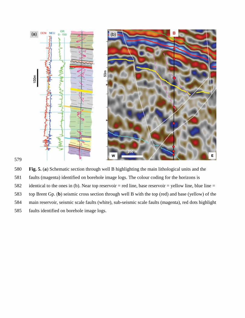
borehole image analysis data (Fig. 5a) suggest a denser fault network (well A = 2 faults/km2, well B = 10 100
faults/km2), which is not represented by a visible offset of horizons at the current seismic resolution. Well 101
A drilled right through one of the faults identified on seismic attribute analysis (Fig. 4). Plotting fault zones 102
identified from borehole image analysis on seismic sections at the well location indicates that many small 103
scale faults are only subtle or not at all visible on the seismic (Fig. 5b). Similar features as in well A are 104
also observed in well B. Very few small-scale faults are recorded in borehole image logs and cores in the 105
southern well C and D at the reservoir level, although those are also located very close to seismic scale 106
faults. No reliable results from the attribute analysis could be obtained due to the poorer quality of the 107
seismic around the two wells. 108
109
Fault rock property analysis 110
Fault rock samples 111
The complete reservoir section has been cored in the wells A and B and the samples analysed in this study 112
were taken entirely from these two cores. Two fault zones with unknown offsets are visible in well A (Fig. 113
6, see also Fig. 5a). It seems appropriate to expect similar fault styles observed in the fault rock samples 114
also at a larger scale in the reservoir-scale faults. Figure 7a shows multiple faults on a small scale, which 115
reflects the observations made on the seismic and borehole images. The fault propagates upwards, 116
nucleating at the lower left and fault splays are developed in the more shale-rich section (between 37m and 117
33cm). The fault continues with a clearly visible offset of a distinctive shale band (29cm). A small clay 118
smear is developed, resulting from the smearing of the fine clay-rich laminations within the sand-rich 119
interval. In the clean sandstones above and below the clay-rich band, the clay content of the fault rock 120
seems to be significantly lower. This is likely to represent the fault rock properties expected in the self-121
juxtaposed cleaner sandstones section for the reservoir scale faults. A small half-graben is present towards 122
the top of Figure 7a, which is infilled with coarser material. The cored faults in more shale-rich layers often 123
show partial clay smear, or at least a clay-rich fault rock (Fig. 7b, c). It is, however, apparent from the 124

sampled faults that clay smears are often discontinuous. It is occasionally observed that the fault dip flattens 125
in the more shale-rich lithologies at the seismic scale (Fig. 3). The same phenomena, caused by 126
geomechanical heterogeneities, is also observed at a small scale in the cored faults, where the dip of the 127
fault surface becomes less steep in the more clay-rich layers (Fig. 8a). Deformation bands are commonly 128
observed features and the fact that no grain fracturing has occurred during faulting indicates that they were 129
formed during shallow burial (Fig. 8b, c). 130
A bias exists for the fault rock samples. In the more heterogeneous section the sample integrity has been an 131
issue, so only faults in the more homogenous, sandier section could be sampled. This implies that faults in 132
impure sandstones and in clay-rich layers are under-represented. 133
134
Analytical procedures 135
Extensive laboratory work was undertaken on selected fault rock samples from two wells (A & B) including 136
CT-scanning, SEM-analysis, absolute permeability analysis, and quantitative XRD (QXRD). The 137
individual techniques are described in more detail below. 138
Sample preparation 139
Typically, 10 to 20 cm sections of core containing the faults were carefully wrapped and sent to the 140
laboratory for analysis. On arrival, the samples were photographed and CT scans were taken using a Picker 141
PQ 2000 medical-style scanner to identify the orientation of faults present and whether or not there were 142
obvious signs of damage generated during coring or following coring. The CT scans allowed us to identify 143
the optimal orientations to take samples for further analysis. A range of subsamples were required for 144
microstructural and petrophysical property analysis of the fault rock present and its associated undeformed 145
sandstone including:- 146
Core plugs of the host and fault rock; the latter were orientated perpendicular to the fault so that 147
fluid was forced to flow across the fault during analysis. It is generally preferred to take 25.4 or 148
38.1 mm core plugs but the core was too thin so 16 and 20 mm core plugs were taken and these 149
were analysed in purpose built core holders. 150
Cubes of fault rock and host sandstone, around 1 to 1.5 cm3, were cut for permeability analysis. 151
The sample containing the fault rock were cut and set in dental putty in an orientation that meant 152
that fluid had to flow through the fault rock during permeability analysis. The use of dental putty 153
means that it is not possible to apply high confining pressures to these samples during permeability 154
analysis. 155

Around 1.5 x 1.5 x 0.5 cm samples containing fault rock and the associated host sandstone were 156
cut for microstructural analysis. 157
A 1cm3 sample representative of the host sandstone was then taken for QXRD analysis. This 158
analysis was not performed on the fault rocks as they were too narrow to be sampled. The fault 159
throws are very low so it was assumed that the mineralogy of the fault is the same as the host 160
sandstone, which is consistent with microstructural observations. 161
All samples were cleaned in a Soxhlet extractor using a 50:50 mixture methanol-toluene/dichloromethane 162
and then dried in a humidity controlled oven at 60oC. 163
SEM analysis 164
The blocks for microstructural analysis were impregnated with a low viscosity resin, ground flat with 165
progressively finer grades of diamond culminating in a polish using 1 たm diamond paste. The samples were 166
then coated with a 10 nm thick layer of carbon before being analysed using a FEI Quanta 650 FEGESEM 167
environmental SEM with Oxford Instruments INCA 350 EDX system/80mm X-Max SDD detector, EBSD 168
and KE Centaurus EBSD system. The mineralogy and diagenetic history of the samples was determined as 169
well as the fault rock microstructure and timing of faulting relative to the diagenetic history. BSEM images 170
were stored as 8 bit TIFF files so that they could be incorporated into an image analysis package and their 171
mineralogy quantified. 172
Permeability analysis 173
Permeability measurements were made using two methods. One set of measurements were made at ambient 174
stress using distilled water as the permeant so the results could be compared to those from previous studies 175
of the permeability of fault rocks (e.g. Fisher & Knipe, 1998; 2001). In these cases, the cleaned cubes were 176
set in dental putty so that they could be confined at 70 psi confining pressure in a steady-state water 177
permeameter. The samples were saturated with distilled water, placed in the permeameter before using 178
syringe pumps to establish steady-state flow. The permeability was calculated using Darcy’s law based on 179
the flow rate, sample length and area, the upstream and downstream pressure differential and the viscosity 180
of the water. The samples containing fault rock also contained undeformed sandstone so the fault 181
permeability was deconvolved from the measurements assuming that the permeability measured was the 182
thickness weighted harmonic average of the fault rock and the host sediment. 183
The second set of measurements were made on core plugs at higher stresses using formation compatible 184
brine. Coreholders were specially constructed for the sample analysis as we could only obtain 16 and 20 185
mm diameter core plugs, which are far narrower than the 25.4 and 38.1 diameter cores normally analysed. 186
The core plugs were trimmed so that the ends were flat and orientated perfectly perpendicular to the axis 187

of the core plug. Formation compatible brine permeabilities were measured under stresses of 500psi, 1500 188
psi, 2000psi, 2500psi, 3000psi, 4000psi, 5000psi. These high stresses close microfractures created as core 189
samples are brought to the surface following coring. Samples with permeabilities of >0.1 mD were 190
measured using the steady-state technique whereas samples with lower permeabilities were measured using 191
the pulse-decay method. As with ambient stress measurements, core plugs containing fault rock also 192
contained undeformed sandstone so the fault permeability was deconvolved from the measurements 193
assuming that the permeability measured was the thickness weighted harmonic average of the fault rock 194
and the host sediment. 195
QXRD analysis 196
The intensity of a X-ray diffraction pattern of a mineral is proportional to the amount present within a 197
mixture (e.g. Hardy & Tucker, 1988). On this basis, XRD has frequently been used to quantify the 198
proportions of minerals present within rocks. One method to make such analyses is to construct calibration 199
curves based on the XRD analysis of mixtures containing different proportions of an internal standard such 200
as corundum. The technique requires preparation of samples with complete random orientation (Brindley, 201
1984). Sample preparation has, however, proved such a difficult task that the technique has been widely 202
regarded as semi-quantitative at best (Hillier, 1999). Recently, a spray dry technique has been developed 203
that appears to produce samples for XRD analysis without significant preferred orientation - even when 204
they contain significant proportions of clays (Hillier, 1999; 2000). The technique involves grinding the 205
sample with a standard (20 wt. % corundum) and then spraying a slurry of the mixture through an air brush 206
into a tube furnace to form ~30 µm wide spherical aggregates with random mineral orientation. The spheres 207
are then top loaded into a specimen holder and then analysed using XRD. The diffraction results obtained 208
are analysed by either reference intensity ratio (RIP) or a Rietvold method to produce mineralogical 209
analyses that are accurate at the 95% confidence level to ±X0.35, where X is the concentration in wt. %. 210
QXRD data is presented as a percentage of the rock volume (including porosity) so is consistent with 211
previous studies (e.g. Fisher and Knipe, 1998, 2001). 212
213
Microstructure, mineralogy and petrophysical property results 214
QXRD analysis indicates that the host sediments contain 54 to 73.4% quartz, 3 to 7.2% albite, 11.4 to 18.7% 215
microcline, 1.4 to 4.4% mica, 1.4 to 17% kaolin and small amounts (<1%) of pyrite. The undeformed 216
sandstones have a diagenetic history that is typical of Jurassic sandstones in the North Sea that have been 217
buried to 2800 m. In particular, they have experienced the precipitation of early K-feldspar overgrowths 218
and kaolin during shallow burial. Mechanical compaction was the main process for reducing porosity and 219

permeability during intermediate burial. The sandstones then experienced small amounts of quartz 220
precipitation and grain contact quartz dissolution. 221
Examination of the structure of the samples in core suggested that most of fault rock samples are 222
phyllosilicate-framework fault rocks (PFFR, Fisher & Knipe, 2001). Microstructural analysis confirms that 223
PFFR are common (Fig. 9) but also indicates that protocataclasites, occasionally with a PFFR border (Fig. 224
10) and to a minor extent cataclasites were also present. In general, many of the samples had 12 to 18% 225
clay, which places them on the border between clean (<15% clay) and impure (>15% clay) sandstones. So 226
the fault rocks that they contained tend to have characteristics of those expected generally formed from 227
clean sandstones (i.e. domains with pore space that is free from clay) whilst other characteristics are typical 228
of faults formed from impure sandstones (e.g. domains with macroporosity being filled by clay as well as 229
having experienced enhanced grain-contact quartz dissolution); this makes a clear classification of the fault 230
rocks difficult. It should be noted that PFFR’s were originally defined as having flow properties that were 231
controlled by presence of a continuous phyllosilicate-rich matrix between the framework grains (Knipe et 232
al., 1997). Later a generalization was made that such fault rocks tend to occur in sandstones containing 15-233
40% clay (Fisher and Knipe, 1998, 2001). However, the clay content of 15-40% should not be viewed as 234
fixed values. Indeed, the discussion on clay mixing models presented below highlights how the sorting of 235
the sand grains, which make up the framework of fault rocks, has a major impact on their petrophysical 236
properties. 237
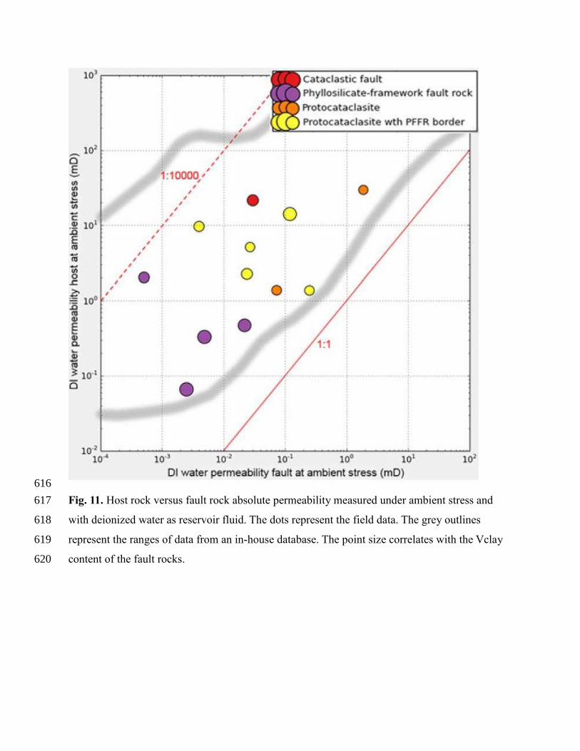
The ratio of the host rock and the fault rock absolute permeabilities is an important parameter that describes 238
the retardation of fluid flow by faults (Yaxley, 1987). Figure 11 shows the data measured from the field 239
and a range of data points from an in-house database from the same area that have the same stratigraphic 240
range and burial depth. Both datasets were measured under ambient stress using distilled water as the 241
permeant. The results demonstrate a permeability reduction of up to three orders of magnitude for the field 242
data. The permeability reductions experienced implies that the fault rocks could have a significant impact 243
on the single-phase flow especially when situated near to a production or injection well. The acquired data 244
from the field fit well into global range, although the permeability reduction seems to be slightly less than 245
in the global dataset. The reduction in permeability occurred as a result of a variety of processes including: 246
faulting-induced grain fracturing, faulting-induced mixing of framework grains with phyllosilicate grains 247
and enhanced grain contact quartz dissolution due to the presence of clays at grain contacts. It is apparent 248
that there is no clear relationship between the fault rock type and the permeability reduction. However, the 249
host rock permeabilties in the more impure sandstones are lower than in the clean sandstones, which is in 250
line with previous work. There does not seem to be a correlation between the clay content of the protolith 251
and the permeability reduction (Fig. 11) although dataset from the field itself is rather limited. 252

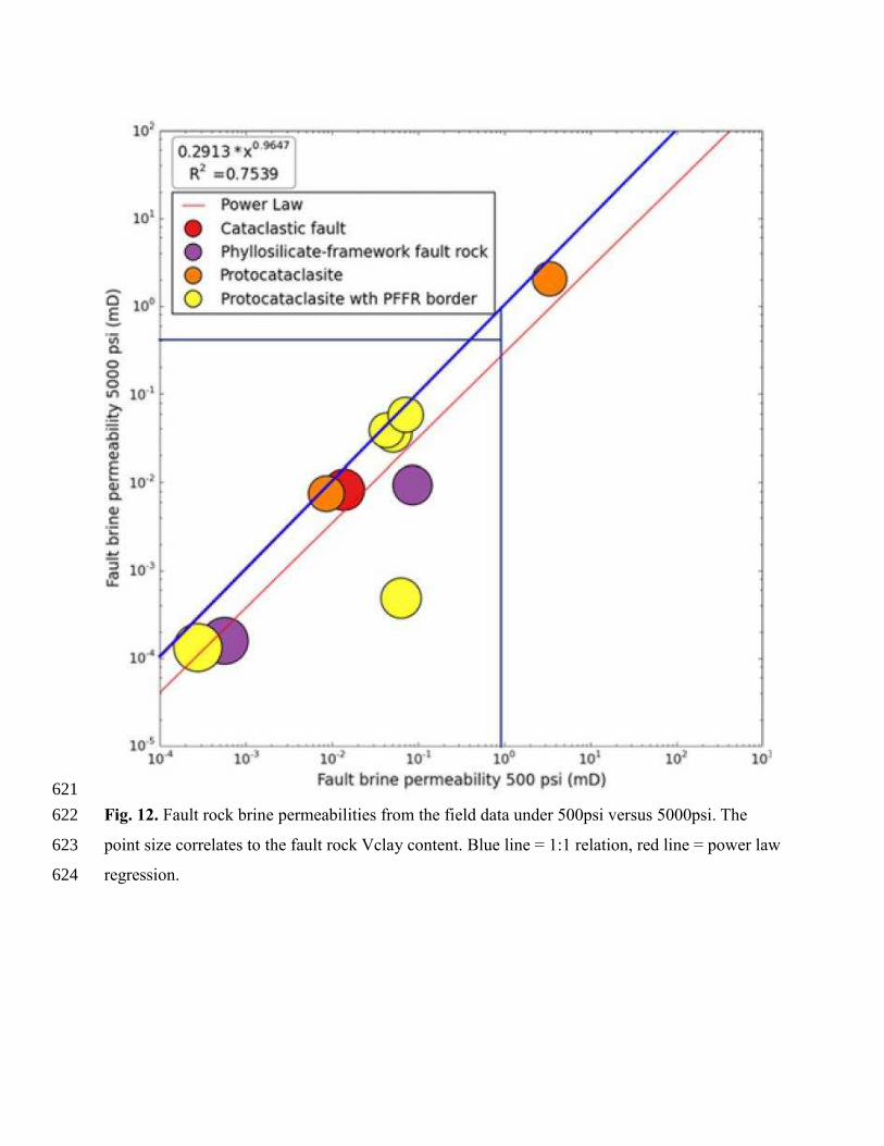
The brine permeability of all fault rocks showed a clear stress dependency (Fig. 9 and Fig. 10). In particular, 253
the stress sensitivity of permeability increases as samples become less permeable (Figure 12). Fault rock 254
samples with >0.1 mD permeability at ambient conditions tend experience permeability reductions of a 255
factor of ~2 when confining pressure is increased to in situ conditions. On the other hand, lower 256
permeability fault rocks often experience an order of magnitude reduction in permeability as confining 257
pressure is increased to in situ conditions. The increased stress dependency of permeability with reduced 258
permeability is consistent with permeability measurements made on other low permeability rocks such as 259
tight gas sandstones (Thomas & Ward, 1972; Wei et al., 1986; Kilmer et al., 1987). Extrapolating the 260
power-law relationship between stress and confining pressure to 70psi indicates that previous 261
measurements made at ambient stress conditions are between 2 and 20 times higher (average difference is 262
5 fold) than those made at high confining pressures. It should be emphasised that much of this stress 263
sensitivity is likely to be caused by presence of grain-scale microfractures that formed during and/or 264
following coring. The permeabilities of fault rock samples are therefore not likely to be as stress sensitive 265
in the subsurface as in the laboratory, because microfractures will not be present in the subsurface and pores 266
with low aspect ratios are not as stress sensitive unless an increase in stress results in brittle failure of the 267
faults. 268
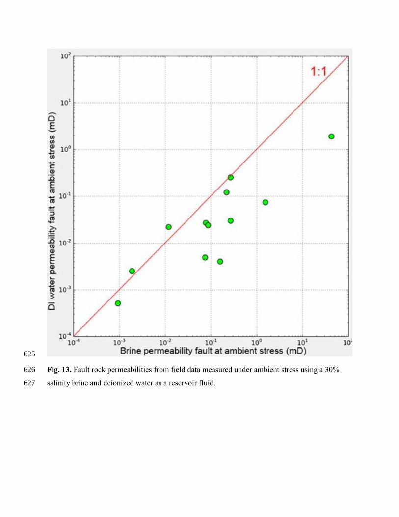
Fault rock permeabilities not only depend on the stress applied, but also on the fluid composition used 269
during the experiments. The data shown in Figure 13 demonstrate that the permeabilities for a formation 270
compatible brine are around 5 fold higher than for a deionized water, which has been used as the permeant 271
for these type of measurements (Fisher & Knipe, 1998, 2001; Sperrevik et al., 2002). 272
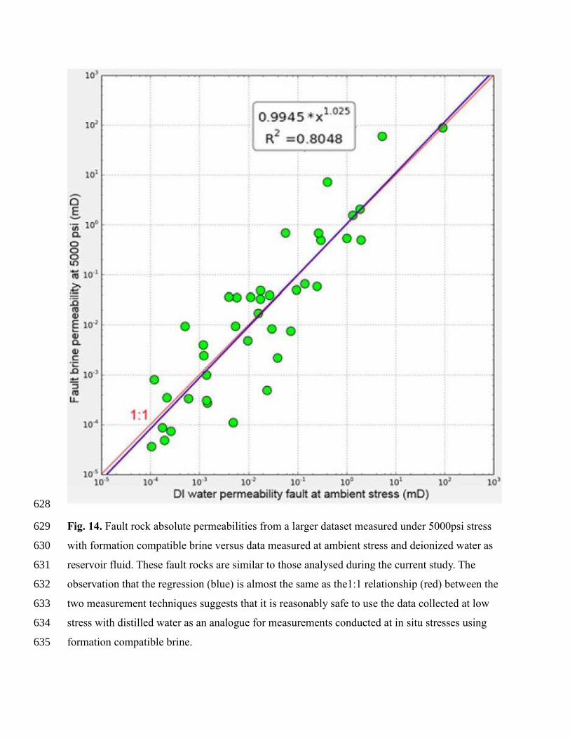
An important observation made during this work, incorporating a larger fault rock data set from different 273
unpublished sources is that the effects of applying reservoir stress versus ambient stress and using brine 274
versus deionized water cancel each other almost out and almost a 1:1 relationship seem to exist (Fig. 14). 275
This implies that previously published fault rock property data (Fisher & Knipe, 1998, 2001; Sperrevik et 276
al., 2002; Jolley et al., 2007) can be still used with a certain confidence. This will be the subject of a future 277
publication but it is important for the current study as it justifies using the legacy fault rock data along with 278
the new measurement from the field to derive predictive functions for the fault rock permeability versus 279
fault rock clay content for the reservoir scale faults. 280
It has been pointed out earlier that a sample bias exists, as some faults, particularly the ones with a higher 281
clay content fault rock or with clay smear, could not be sampled, as the samples tend to break apart along 282
the faults. So the sampled fault rocks mainly resemble the low to medium clay content fraction with some 283
that show properties of phyllosilicate-framework fault rocks (Fig. 15). A relationship between the fault rock 284
type and the fault rock permeability exists, despite the fact that differences in permeabilities of up to two 285
orders of magnitude exist for a similar fault rock clay content are measured (Fig. 15). This observation is 286
consistent with earlier published datasets (Fisher & Knipe, 2001; Sperrevik et al., 2002; Jolley et al., 2007). 287
288
Reservoir-scale fault property prediction 289
To calculate the reservoir and small-scale (lineaments from seismic attribute analysis, see Fig. 4) fault 290
properties a structural framework and a static geomodel has been established. The basis for the model is 291
provided by 3D structural interpretation on a PreSDM dataset and a host rock Vclay model based on the 292
Vclay logs from the four exploration wells, applying an appropriate depositional model. The fault rock 293
clay content has been calculated varying the clay content of the host rock model according to the 294
uncertainties from the petrophysical evaluations. Different fault zone clay predictors, such as SGR 295
(Yielding, 2002) and ESGR (Freeman et al., 2010) were assessed. The SGR at any point of the fault is 296
given by a uniform average of the clay contents of the wall rocks that moved past this point (Yielding 2002). 297
In contrast, the ESGR applies an additional weighting function to the averaging, which assumes that clays 298
that are closer to the point of interest contribute more to the fault rocks (Freeman et al., 2010). To link the 299
fault rock permeability to the fault rock Vclay content; SGR/ESGR for reservoir scale faults; different 300
predictive functions were applied. In addition the impact of potential clay smear on the production figures 301
has been evaluated, together with changes in the relationship of fault rock thickness versus fault throw. 302
Variations in fault throw can have a significant effect on the fault rock properties and reservoir/reservoir 303
juxtaposition patterns in the field. Therefore an uncertainty on the throw of 20% has been incorporated. 304
The majority of the reservoir-scale faults fall into the PFFR domain, followed by clay smears and 305
disaggregation zones/(proto)cataclastic fault rocks (Fig. 17). No significant difference in the distribution is 306
apparent between the fault rock Vclay content when calculated using either SGR (Yielding, 2002) or ESGR 307
(Freeman et al., 2010), with a weighting factor of 1.5, as a fault rock Vclay prediction algorithm. A more 308
detailed analysis of the Vclay distribution on the fault plane reveals that the ESGR algorithm predicts a 309
more discrete distribution of Vclay, compared to the SGR algorithm (Fig. 17). The aim was to verify the 310
influence of the application of the two different algorithms on the final dynamic simulation results. 311
The fault rock property data acquired during this study are limited in terms of their statistical value as only 312
around 15 samples of small offset faults (<1 cm throw) were analysed and they do not represent the range 313
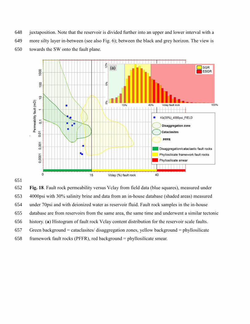
of reservoir scale fault rocks (see Fig. 16). To have a statistically valid dataset the field data were combined 314
with data from an in-house database, obtained from the same province, same stratigraphic interval and 315
similar burial depth (Fig. 18). The measurements for the additional data were done under 70psi stress and 316
with deionized water as reservoir fluid, which has discussed above are probably fine to use as the use of 317

distilled water appears to compensate for the impact on permeability of making the measurements at low 318
confining pressures. A cross-plot of fault rock permeability vs. clay content for this larger dataset from 319
analogue faults also has a very large amount of scatter as was the case for the measurements made during 320
this study. 321
Revil & Cathles (1999) demonstrate that the permeability of the sand/clay mixtures, which is essentially 322
what clay gouges represent, is controlled by the proportion of the host-rock sand and host-rock clay present, 323
the porosity and permeability of the sand end-member as well as the permeability of the shale end-member. 324
The porosity of the host-rock sand is controlled by grain sorting. These factors might explain the scatter of 325
the points in the Vclay versus permeability plot (Fig. 18). The objective was to represent the ranges between 326
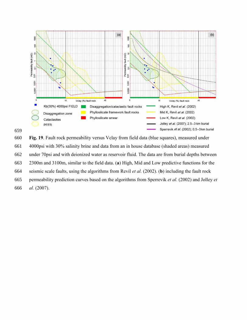
fault rock Vclay content and fault rock permeability for the reservoir scale faults. A High-, Mid- and Low-327
fault rock permeability predictive function has been established (Fig. 19a). The functions are based on a 328
model for the permeability of clay-sandstone mixtures (倦陳岻, presented by Revil et al. (2002). 329
330 倦陳 噺 倦鎚鳥怠貸蝶迩如叶濡匂 抜 倦寵捗鎚蝶迩如【叶濡匂 ┸ ど 判 撃頂鎮 判 叶鎚鳥 331
332 倦陳 噺 倦鎚朕撃頂鎮戴【態┸ 叶鎚鳥 判 撃頂鎮 判 な 333
334
where, øsd and ksd are the porosity and permeability of the clay-free sand, ksh is the permeability of the 335
shale end-member and: 336 倦寵捗鎚 噺 倦鎚朕叶鎚鳥戴【態 337
338 撃頂鎮 is the clay content of the fault rock┸ e┻ g┻ SGR or ESGR for the reservoir scale faults and 倦寵捗鎚 is the 339
permeability of the clay-filled sand at the boundary between the clayey sands and sandy shales (Revil et 340
al., 2002). The three functions were calculated by establishing three sand-clay mixing models, using the 341
parameters in Table 1. A good fit to the data for the three functions becomes apparent (Fig. 19a). The field 342
data, despite there are only few, fall clearly within the Mid- and Low-case scenario from Revil et al. (2002). 343
Comparing the Revil et al. ( 2002) High, Mid and Low fault rock permeability functions with algorithms 344
published previously by Sperrevik et al. (2002) and Jolley et al. (2007) for similar conditions (burial depth 345
<3000m) , it becomes apparent that the latter predict a higher permeability of the fault rocks than indicated 346
by the field data (Fig. 19b). 347
The final input parameter into the reservoir simulator are TMs that are applied to the faces of grid blocks 348
on either side of the fault plane to take into account the impact of faults on fluid flow. The TM calculation, 349
as described by Manzocchi et al. (1999), requires information on the permeability of the undeformed 350
reservoir in each grid block, the fault thickness and the fault permeability. The prediction of the fault rock 351
thickness is one of the most uncertain parameters. There is a significant scatter in the data, but a 1:100 352
relationship of fault thickness versus throw is commonly used. Freeman et al. (2008) suggest that a 1:66 353
relationship is more appropriate for seismic-scale faults. Both relationships were incorporated into the 354
calculation of the fault TMs. 355
An uncertainty also exists in the calculation of the Vclay content for the well logs and hence for the Vclay 356
model as such. A 10% uncertainty has been estimated, based on petrophysical analysis, for the host rock 357
Vclay content and fault rock property cases were calculated accordingly. In addition potential facies 358
variations were taken into consideration in the uncertainty modelling. 359
Many properties are linked to the fault throw, such as the reservoir juxtaposition pattern, fault rock clay 360
content prediction, the fault rock thickness and ultimately the TM, as the main input into the dynamic 361
simulation. The fault throw is influenced by three main factors, the accuracy of the seismic migration, the 362
quality and resolution of the seismic data and the structural interpretation. In this case, an uncertainty of the 363
throw of 20% has been considered, based on the above mentioned parameters. A variation of the throw in 364
the static geomodel alters the model geometry and sometimes it is difficult to carry this distorted geometry 365
forward in the dynamic simulation. In order to keep the complexity at an acceptable level, it has been 366
decided to calculate only one case for the throw variation, e.g. increase the throw by 20% (throw 120%). 367
An increase in throw is expected to result in a more disconnected reservoir, which would decrease the 368
recoverable volumes and demonstrates a potential “low case” scenario. The effective-cross fault 369
transmissibility (ECFT, Freeman et al., 2010) is used in Figure 20 to illustrate the effects of an increase in 370
throw. The ECFT, which is a normalized cross fault transmissibility, is computed using the harmonic 371
average of the permeabilities of the undeformed foot wall adjacent to the fault, the fault rock and the 372
undeformed hanging wall across the fault. This is done for a specific width of host wall rock on each side 373
of the fault and the fault rock thickness by the local displacement (Freeman et al., 2010). The lower reservoir 374
interval is the one that contributes most to the recoverable volumes. An increase in throw reduces the area 375
where the lower reservoir is self-juxtaposed (Fig. 20a & b). The fact that more zones with elevated ECFT 376
in the area where the lower reservoir in the footwall is juxtaposed against the upper reservoir in the 377
hangingwall occur (compare Fig. 20a and Fig. 20b), does not counterbalance this effect. This becomes 378
evident in the dynamic simulation. 379
380
381
Small scale fault property prediction 382
In addition to the seismic faults numerous small-scale faults, without a visible offset in seismic exist. These 383
faults can be observed as lineaments on seismic attribute maps (Fig. 4). It has been considered to be 384
important to include these faults into the dynamic simulation model. The faults were mapped as lineaments 385
and vertical fault planes without an offset were constructed in the dynamic model. As no offset is associated 386
with these faults, their TMs cannot be calculated in the same way as for faults with an offset. Therefore a 387
range of single TMs for the entire small scale fault surfaces was calculated, applying a range of fault throw 388
(1m, 5m, 10m, 20m) with the corresponding fault rock thicknesses using a thickness to throw relationship 389
of 1:100. A single average permeability value of 950 mD has been taken for footwall and hangingwall cells, 390
based on a range of core measurements in the reservoir sandstones. A bulk fault zone permeability has been 391
calculated using the harmonic average from the measured fault rock permeabilities from the cores, using a 392
30% salinity brine and applying a stress of 4000psi. The harmonic average was used as the permeability 393
required is that measured perpendicular to the fault. It has been concluded from applying the different 394
scenarios that bulk TMs of 0.001, 0.01 and 0.1 represent a realistic range for the small scale faults. 395
At this stage of the analysis it is important to bear in mind that no history matching data exist in the field, 396
which would allow a calibration of the results. It is important at this point in time to figure out which 397
parameters have the most significant impact on the resulting recoverable volumes. Once history matching 398
data are available this provides a good basis for a more focused analysis of the key influencing parameters. 399
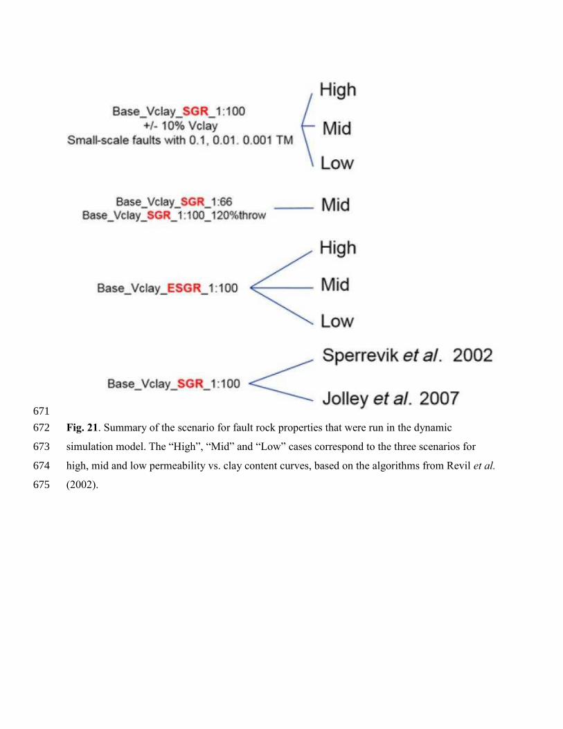
A summary of the cases that were incorporated into the dynamic simulation is given in Figure 21. 400
401
Simulation modelling results 402
The scenarios discussed above were, together with other geological variables, incorporated into a fully 403
integrated, automated workflow for dynamic reservoir simulation and uncertainty modelling (200 404
iterations). The main goal was to identify which one of the many parameters, apart from the fault properties, 405
in the uncertainty model have the most impact on the recoverable volumes and the recovery efficiency. An 406
additional objective was to verify the impact of the different fault property cases on the recoverable volume 407
range. In order to ensure that the results are comparable, the producer/injector well pattern has not been 408
changed during the uncertainty simulation. 409
In Figure 22 the impact of the several calculated scenarios on the recoverable volumes is highlighted. In 410
case a TM = 1 is applied, the recoverable volumes are as if there were no faults present, e.g. normalized to 411

100%. If the minimum case of recoverable volumes is valid, e.g. if low permeable seismic scale faults 412
combined with low permeable small scale faults are present, the recovery would be only 70% compared to 413
a model without faults. The dynamic simulation reveals that the clay content versus permeability 414
relationship, together with variations in fault throw, have the most significant impact on the recoverable 415
volumes (Fig. 22). Slightly tighter faults are predicted when the ESGR is used as a mixing algorithm. The 416
impact of a thickness to throw ratio of 1:66 instead of 1:100 leads to a decrease in fault transmissibility, but 417
not to a significant amount. The presence of clay smear does not lead to significantly tighter faults and 418
hence causes only a minimal reduction in recoverable volumes because continuous clay layers are not 419
predicted in the host rock model. The functions suggested by Sperrevik et al. (2002) and Jolley et al. (2007) 420
seem to predict less influence of the faults on the subsurface fluid flow for this particular case. The 421
incorporation of small-scale faults whose throw cannot be mapped can decrease the recoverable volumes 422
again by up to 10%, compared to the cases where only the larger scale faults are taken into consideration. 423
Combining the observations made on core-scale, with seismic attribute analysis strongly suggests the need 424
to incorporate the small-scale faults into the model. The dynamic simulation with several fault property 425
scenarios shows that a reduction between 10% and 30% of the recoverable volumes, compared to a model 426
without or completely open faults, is likely. 427
The impact of the faults on the recovery efficiency and cumulative production were assessed in the 428
uncertainty modelling. Apart from the fault properties, other parameters such as the variation on top and 429
base reservoir grids, residual oil and water saturation and reservoir porosity and permeability were 430
incorporated into the analysis. The properties of the faults are among the most influential parameters for 431
the oil recovery efficiency. Using fault specific TMs, generated applying the above discussed workflow, 432
versus a distribution of single TM values reduces the uncertainty by around 40% for the recovery efficiency. 433
This is a very important result as it clearly demonstrates the value of a detailed fault analysis compared to 434
just using single global values. 435
For the cumulative production the fault properties are an important, but not the most influential parameter. 436
Again, using a fault specific TM grid, based on the above described fault analysis workflow, compared to 437
applying a range of single TM reduces the uncertainty by 50%. 438
439
Discussion 440
The seismic interpretation, which is a key element that provides the basis for a quality fault analysis and 441
the translation of the interpretation into the static geomodel, has not been discussed in detail in this paper. 442
The seismic data quality across the field is only fair, which implies that that the fault and horizon picking 443
is associated with uncertainties; the same is also true for the velocity model. The possibility to run fully 444
integrated uncertainty models really helped to incorporate these different parameters and assess their 445
impact. However, a verification of effects from different interpretation concepts is not possible within this 446
workflow, but would be a subject for further analysis, once the field is in development and history 447
matching data exist, which allow a better calibration of the outcomes. 448
Similar fault styles are observed on core and seismic scale (compare Figure 2 with Figure 8). The 449
availability of numerous fault rock samples from core, together with high quality borehole images was a 450
real benefit for the work. In the first instance, these data highlight the complexity of the faulting, also 451
below seismic resolution. Secondly, the fault rock data provide the basis for the calibration of the 452
reservoir-scale fault rock permeability prediction. As demonstrated, the results from the absolute 453
permeability measurements on these samples under reservoir stress conditions, using a reservoir 454
compatible fluid are very similar to absolute permeability measurements under ambient stresses but using 455
deionized water as a permeant (Fig. 14). It shall be pointed out, that this observation does not imply that 456
the efforts for conducting measurements under realistic subsurface conditions are not necessary in the 457
future, but highlights the possibility to use previously acquired datasets with a certain confidence. 458
We find that the functions developed by Revil et al. (2002) provide an appropriate description for sand-459
clay mixtures (fault rocks) and their related absolute permeabilities. Revil & Cathles (1999) demonstrate 460
that the permeabilities of these mixtures are not only a function of the clay content, as suggested by 461
previous authors (Fisher& Knipe 1998; Fisher & Knipe 2001). Functions that correlate the fault rock clay 462
content to the fault rock permeability suggested by Sperrevik et al. (2002) and Jolley et al. (2007) seem to 463
predict a lower impact of the faults on the subsurface fluid flow in this specific case. This can be due to 464
various factors including: 465
i. The functions suggested by Jolley et al., (2007) and Sperrevik et al., (2002), which were used in this 466
paper for comparison, are derived from regression lines through a cloud of data with a significant 467
scatter for a given depth of burial. This implies that the high- and low-side will not be fully 468
represented. 469
ii. The measurement setup, e.g. permeability measurements with deionized water at ambient stress 470
does not represent real subsurface conditions, e.g. reservoir compatible brine at subsurface stress. 471
iii. The data used by Jolley et al. (2007) and Sperrevik et al. (2002) are not from the field, so the use of 472
specific field data should provide more accurate ranges. 473
iv. The sand-clay mixing model proposed by Revil & Cathles (1999) appears to be a proper 474
representation of the parameters that lead to the development of fault rocks and their properties.. 475
It has been pointed out already that the work described in this paper lacks the calibration of the fault 476
analysis results by history matching data or even long term well tests. Once the field is under 477
development and production data exist, the exercise will have to be repeated and it is expected that the 478
uncertainties can be significantly reduced. In any case, the current study provides a good basis for future 479
work. 480
481
Conclusions 482
A better understanding of the fault properties by incorporating geologically sensible parameters played an 483
important role in the uncertainty assessment for the field development planning. In this context the 484
incorporation of fault rock measurements from field data, together with application of the algorithms from 485
Revil et al. (2002) for the fault rock clay content prediction increased significantly the credibility of the 486
analysis results. The fault properties are among the most critical and influential parameters especially for 487
the recovery efficiency, but also for the cumulative production. It can be demonstrated that using a fault 488
specific transmissibility multiplier grid versus a distribution of single, global transmissibility multiplier 489
values significantly reduces the uncertainties for the recovery efficiency and cumulative recovery. 490
491
Acknowledgements 492
The authors thank Wintershall Norge AS, Capricorn Norge AS, Bayerngas Norge AS, DEA Norge AS, 493
Repsol Norge As, Edison Norge AS and Explora Petroleum AS, for the permission to publish this paper. 494
We also thank Eriksfiord and the CiPEG Leeds for the permission to present data generated by them for 495
this study. 496
497
References 498
Brindley, G.W. (1984) Quantitative X-ray analysis of clays. Pp. 411-438 in: Crystal Structures of Clay 499
Minerals and their X-ray Identification (G.W. Brindley & G. Brown, editors). Mineralogical Society, 500
London. 501
Fisher, Q. J. & Knipe, R. J. 1998. Fault sealing processes in siliciclastic sediments. In: G. Jones, Q. Fisher 502
and R. J. Knipe (eds) Faulting and Fault Sealing in Hydrocarbon Reservoirs. Geological Society, London, 503
Special Publication, 14, 117-134. 504
Fisher, Q. J. & Knipe, R. J. 2001. The permeability of faults within siliciclastic petroleum reservoirs of 505
the North Sea and Norwegian Continental Shelf. Marine and Petroleum Geology, 18, 1063-1081. 506
Fisher, Q.J. & Jolley, S.J. 2007. Treatment of faults in production simulation models. In: Jolley, S. J., 507
Barr, D., Walsh, J. J. & Knipe, R. J. (eds) Structurally Complex Reservoirs. Geological Society, London, 508
Special Publications, 292, 219-233. 509
Freeman, S.R., Harris, S.D. & Knipe, R.J. 2008. Fault seal mapping – incorporating geometric and 510
property uncertainty. In: Robinson, A., Griffiths, P., Price, S., Hegre, J. & Muggeridge, A. (eds) The 511
Future of Geological Modelling in Hydrocarbon Development. The Geological Society, London, Special 512
Publications, 309, 5-38. 513
Freeman, S.R., Harris, S.D. & Knipe R.J. 2010. Cross-fault sealing, baffling and fluid flow in 3D 514
geological models: tools for analysis, visualization and interpretation. Geological Society, London, 515
Special Publications, 347, 257-282. 516
Hardy, R. & Tucker, M.E. 1988. X-ray diffraction. In: Tucker, M. E. (eds) Techniques in Sedimentology. 517
Blackwell, Oxford, 191-228. 518
Hillier, S. 1999. Use of an Air Brush to Spray Dry Samples for X-Ray Powder Diffraction. Clay 519
Minerals, 34, 127-135. 520
Hillier, S. 2000. Accurate quantitative analysis of clay and other minerals in sandstones by XRD: 521
comparison of a Rietveld and a reference intensity ratio (RIR) method and the importance of sample 522
preparation. Clay Minerals, 35, 291-302. 523
Jolley, S.J., Dijk, H., Lamens, J.H., Fisher, Q.J., Manzocchi, T., Eikmans, H. & Huang, Y. 2007. Faulting 524
and fault sealing in production simulation models: Brent Province, northern North Sea. Petroleum 525
Geoscience, 13, 321-340. 526
Kilmer, N.H., Morrow, N.R., and Pitman, J.K. 1987. Pressure sensitivity of low permeability sandstones. 527
Journal of Petroleum Science and Engineering, 1, 65-81. 528
Knipe, R. J., Fisher, Q. J., Jones, G. , Clennell, M. R., Farmer, A. B., Kidd, B., McAllister, E., Porter, J. R. 529
& White, E. A. 1997. Fault seal analysis, successful methodologies, application and future directions. In: 530
Møller-Pederson, P. & Koestler, A. G. (eds) Hydrocarbon Seals - Importance for Exploration and 531
Production. Norwegian Petroleum Society (NPF), Special Publication, 7, 15-37. 532
Lever A., and Dawe, R.A. 1987. Clay migration and entrapment in synthetic porous media. Marine 533
and Petroleum Geology, 4, 112-118. 534
Manzocchi, T., Walsh, J.J., Nell, P. & Yielding, G. 1999. Fault Transmissibility Multipliers for flow 535
simulation models. Petroleum Geoscience, 5, 53–63. 536
Revil, A. & Cathles L.M. 1999. Permeability of shaly sands. Water Resources Research, 35, 651-662. 537
Revil, A.C., Grauls, D. & Brevart, O. 2002. Mechanical compaction of sand/clay mixtures, Journal of 538
Geophysical Research, 107, (B11), 2293. 539
Sperrevik, S., Gillespie, P.A., Fisher, Q.J., Halvorsen, T. & Knipe, R.J. 2002. Emperical Estimation of 540
Fault Rock Properties. In : Koestler, A. G. & Hunsdale, R. (eds) Hydrocarbon Seals Quantification. 541
Norwegian Petroleum Society (NPF), Special Publication, 11, 109-125. 542
Thomas, R.W. & Ward, D.C. 1972. Effect of Overburden Pressure and Water Saturation on Gas 543
Permeability of Tight Sandstone Cores, JPT, 120. 544
Wei, K.K., Morrow, N.R. & Brower, K.R. 1986. Effect of Fluid, Confining Pressure, and Temperature on 545
Absolute Permeabilities of Low-Permeability Sandstones, Society of Petroleum Engineers, Formation 546
Evaluation, 413. 547
Yaxley, L.M., 1987. Effect of a partially communicating fault on transient pressure behaviour. Society of 548
Petroleum Engineers, Formation Evaluation, 590–598. 549
Yielding, G. 2002. Shale gouge ratio – calibration by geohistory. In : Koestler, A. G. & Hunsdale, R. 550
(eds) Hydrocarbon Seals Quantification. Norwegian Petroleum Society (NPF), Special Publication, 11, 1-551
15. 552
553
554
Figure captions 555

556
Fig. 1 (a) Top reservoir depth map with the four exploration/appraisal wells (A-D) and the fault 557
polygons (b) 3D fault model from the static geological model (view from above), colored areas 558
(SGR) highlight reservoir/reservoir juxtaposition. 559
560
Fig. 2. Depth seismic section across the field, highlighting the structural complexity at reservoir 561
level. Note that most faults predate the unconformity (red horizon), but some also seem to have 562
younger movements. Green horizon = Base Crecateous Unconformity, red horizon = near top 563
reservoir and unconformity, yellow horizon = base reservoir, blue horizon = Top Brent Gp. 564
565
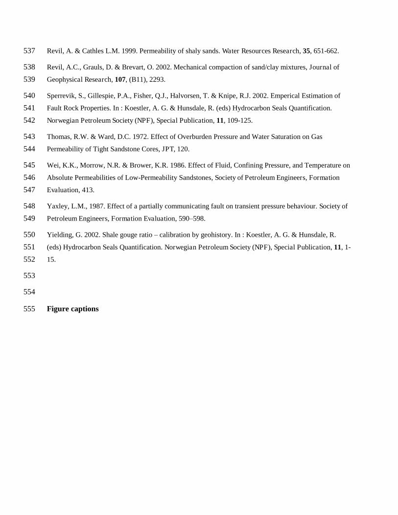
Fig. 3. Depth seismic section across the field, highlighting the structural complexity at reservoir 566
level. Note that most faults predate the unconformity (red horizon), but some also seem to have 567
younger movements. Note the thickening across the faults (white arrows), indicating syntectonic 568
deposition. Occasionally a dip refraction of the faults in the more shale rich lithologies between 569
the base reservoir and top Brent Gp is visible. Green horizon = Base Cretaceous Unconformity, 570
red horizon = near top reservoir and unconformity, yellow horizon = base reservoir, blue horizon 571
= Top Brent Gp. 572
573
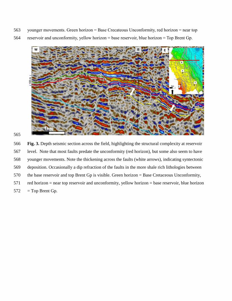
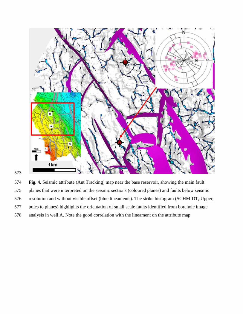
Fig. 4. Seismic attribute (Ant Tracking) map near the base reservoir, showing the main fault 574
planes that were interpreted on the seismic sections (coloured planes) and faults below seismic 575
resolution and without visible offset (blue lineaments). The strike histogram (SCHMIDT, Upper, 576
poles to planes) highlights the orientation of small scale faults identified from borehole image 577
analysis in well A. Note the good correlation with the lineament on the attribute map. 578
579
Fig. 5. (a) Schematic section through well B highlighting the main lithological units and the 580
faults (magenta) identified on borehole image logs. The colour coding for the horizons is 581
identical to the ones in (b). Near top reservoir = red line, base reservoir = yellow line, blue line = 582
top Brent Gp. (b) seismic cross section through well B with the top (red) and base (yellow) of the 583
main reservoir, seismic scale faults (white), sub-seismic scale faults (magenta), red dots highlight 584
faults identified on borehole image logs. 585
586

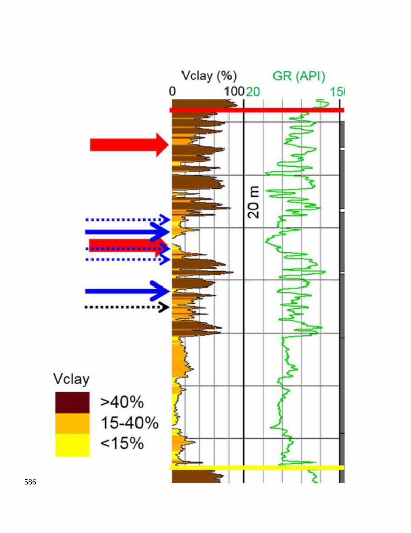
Fig. 6. Reservoir section from well B with Vclay and GR log. Bold red arrows = fault zones 587
identified on image log. Solid blue arrows = fault rock samples displayed in Fig. 10 & 11. 588
Stippled blue arrows = additional sampled and analyzed fault rocks. Stippled black arrow = 589
sample in Figure 7c. Red line = top reservoir, yellow line = base reservoir. The grey section on 590
the right side of the log represents the cored intervals. 591
592
Fig. 7. Cored small scale faults (a) Multiple normal faults. (b) Single normal fault with cm-offset 593
of a clay-rich layer. The dark colored fault rock is enriched with phyllosilicates. (c) Normal fault 594
with a cm-offset of a shale layer, developing a clay smear (white arrow); see also Figure 6 for 595
location. 596

597
Fig. 8. Cored small scale faults and deformation bands (a) Small scale normal faults with cm-598
offset. Note the influence of the mechanical stratigraphy on the dip-angle of the fault plane. (b) 599
Normal faulting in a clay-rich layer and deformation bands without visible offset in a clean 600
sandstone package. (c) Deformation bands in a clean sandstone section. The dark color is due to 601
trapped oil, which cannot escape due to the reduced porosity. 602

603
Fig. 9. Phyllosilicate framework fault rock (PFFR) in an impure sandstone. The offset of the 604
fault is not visible. (a) core sample with a white arrow showing the position from where the 605
sample for laboratory analysis was taken. (b) Results from absolute gas and brine permeability 606
measurements from the host and fault-rock under different stresses. Note the stress-related 607
permeability reduction. (c) BSEM image from host rock (d) BSEM image from fault rock. 608

609
Fig. 10. Protocataclasite with PFFR border in a clean sandstone. The offset of the fault is not 610
visible (a) core sample with a white arrow showing the position from where the sample for 611
laboratory analysis was taken. (b) Results from absolute gas and brine permeability 612
measurements from the host and fault-rock under different stresses. Note the stress-related 613
permeability reduction. (c) BSEM image from host rock (d) BSEM image from fault rock; note 614
the PFFR border ( green arrow). 615
616
Fig. 11. Host rock versus fault rock absolute permeability measured under ambient stress and 617
with deionized water as reservoir fluid. The dots represent the field data. The grey outlines 618
represent the ranges of data from an in-house database. The point size correlates with the Vclay 619
content of the fault rocks. 620
621
Fig. 12. Fault rock brine permeabilities from the field data under 500psi versus 5000psi. The 622
point size correlates to the fault rock Vclay content. Blue line = 1:1 relation, red line = power law 623
regression. 624
625
Fig. 13. Fault rock permeabilities from field data measured under ambient stress using a 30% 626
salinity brine and deionized water as a reservoir fluid. 627
628
Fig. 14. Fault rock absolute permeabilities from a larger dataset measured under 5000psi stress 629
with formation compatible brine versus data measured at ambient stress and deionized water as 630
reservoir fluid. These fault rocks are similar to those analysed during the current study. The 631
observation that the regression (blue) is almost the same as the1:1 relationship (red) between the 632
two measurement techniques suggests that it is reasonably safe to use the data collected at low 633
stress with distilled water as an analogue for measurements conducted at in situ stresses using 634
formation compatible brine. 635

636
Fig. 15. Fault rock brine permeability under 5000psi stress plotted against the fault rock clay 637
content. 638

639
Fig. 16. Histogram plot of fault rock Vclay content for the reservoir scale faults based on a base 640
case Vclay geomodel and a base case fault throw. The difference applying the SGR (Yielding, 641
2002) and ESGR (Freeman et al., 2010) algorithm as a fault rock Vclay predictor is shown. The 642
ESGR is for a hangingwall and footwall combination with a weighting factor of 0.15. 643
644
Fig. 17. Calculated fault rock Vclay content applying two different fault rock Vclay prediction 645
algorithms (a) SGR (b) ESGR. (c) Near top reservoir map with seismic scale faults. The area 646
colour coded with fault properties on ‘a’ and ‘b’corresponds to the reservoir-reservoir self-647
juxtaposition. Note that the reservoir is divided further into an upper and lower interval with a 648
more silty layer in-between (see also Fig. 6); between the black and grey horizon. The view is 649
towards the SW onto the fault plane. 650
651
Fig. 18. Fault rock permeability versus Vclay from field data (blue squares), measured under 652
4000psi with 30% salinity brine and data from an in-house database (shaded areas) measured 653
under 70psi and with deionized water as reservoir fluid. Fault rock samples in the in-house 654
database are from reservoirs from the same area, the same time and underwent a similar tectonic 655
history. (a) Histogram of fault rock Vclay content distribution for the reservoir scale faults. 656
Green background = cataclasites/ disaggregation zones, yellow background = phyllosilicate 657
framework fault rocks (PFFR), red background = phyllosilicate smear. 658
659
Fig. 19. Fault rock permeability versus Vclay from field data (blue squares), measured under 660
4000psi with 30% salinity brine and data from an in house database (shaded areas) measured 661
under 70psi and with deionized water as reservoir fluid. The data are from burial depths between 662
2300m and 3100m, similar to the field data. (a) High, Mid and Low predictive functions for the 663
seismic scale faults, using the algorithms from Revil et al. (2002). (b) including the fault rock 664
permeability prediction curves based on the algorithms from Sperrevik et al. (2002) and Jolley et 665
al. (2007). 666

667
Fig. 20. Effect of increase in fault throw on ECFT (Freeman et al., 20010). (a) base case throw. 668
(b) 20% increase of fault throw. Note the reduction of the area with high ECFT (black arrow) 669
where the lower reservoir is self-juxtaposed. See discussion in text. 670
671
Fig. 21. Summary of the scenario for fault rock properties that were run in the dynamic 672
simulation model. The “High”, “Mid” and “Low” cases correspond to the three scenarios for 673
high, mid and low permeability vs. clay content curves, based on the algorithms from Revil et al. 674
(2002). 675

676
Fig. 22. Imapct of different fault properties scenarios on recoverable volumes, thickness to throw 677
ratio of 1:100, except case 4 with 1:60; 1&5)High_K, 2&6) Mid_K, 3&7) Low_K, 4) Mid_K with 678
thickness to throw ratio of 1:66, 6* & 2*) same as case 2 and 6, but taking into account the potential 679
of clay smear in addition to the fault gouge, 8) Jolley et al.,2007, 9) Sperrevik etal., 2002, 2**) 680
Mid_K case 2 with 20% increase in throw. Note the impact of incorporating the small scale faults 681
on the recoverable volume range. A bulk transmissibility multiplier of 0.1, 0.01 and 0.001 has been 682
assigned to the small scale faults. Note that all cases, except 8 and 9 use the mixing algorithms 683
from Revil et al. (2002) to calculate the fault rock permeabilities. The SGR is used as a fault rock 684
Vclay prediction for 8 & 9. The Y-axis is dimensionless. 685
686
Table 1. Input values for the High, Mid, Low fault rock permeability predictive functions. The 687
porosities and permeabilities in the High, Mid and Low rows correspond to the sandstones. Note 688

that these are host rock parameters, which are used in the mixing model proposed by Revil et al. 689
(2002). 690
691
692
693