i

THE VALUATION OF CREDIT DEFAULT SWAPS

by

Nafi Colette Diallo

A thesis submitted in partial fulfillment of the requirements for the degree of

Professional Masters Degree in Financial Mathematics

Worcester Polytechnic Institute

2005

Approved by LUIS J. ROMAN______________________________________ Chairperson of Supervisory Committee

__________________________________________________

__________________________________________________

__________________________________________________

Date __________________________________________________________

1

WORCESTER POLYTECHNIC INSTITUTE

The Valuation of Credit Default Swaps

by Nafi Colette Diallo

Chairperson of the Supervisory Committee: Luis J. Roman Mathematical Sciences

2

Table of Contents ............................................................................................................... 2

Acknowledgments .............................................................................................................. 3

Introduction ......................................................................................................................... 4

Credit Risk............................................................................................................................ 5

1.1. MODELING CREDIT RISK.................................................................................... 6

1.2. MANAGING CREDIT RISK .................................................................................16

Credit Default Swaps........................................................................................................ 24

2.1. CORPORATE CDS....................................................................................................26

2.2. ASSET-BACKED CDS (ABCDS) ..........................................................................28

2.3. CDS AS RISK MANAGEMENT TOOL .............................................................29

2.4. ASSET-BACKED CDS VALUATION.................................................................30

Data and Methods ............................................................................................................ 36

3.1. THE HAZARD RATE METHOD USING

BOOTSTRAPPING .................................................................................................................36

3.2. RESULTS AND DISCUSSION..............................................................................40

Conclusion.......................................................................................................................... 45

References .......................................................................................................................... 46

3

ACKNOWLEDGMENTS

I dedicate this work to my parents and my brother- may their souls rest in peace-,

and to all those who, directly or indirectly, have helped me and supported me all

these years.

I would like to thank my advisor for all the patience and guidance, my PhD office

mates, all my teachers, my classmates for all the support and advice.

4

INTRODUCTION

The credit derivatives market has known an incredible development since its

advent in the 1990’s. Today there is a plethora of credit derivatives going from

the simplest ones, credit default swaps (CDS), to more complex ones such as

synthetic single-tranche collateralized debt obligations. Valuing this rich panel of

products involves modeling credit risk. For this purpose, two main approaches

have been explored and proposed since 1976. The first approach is the Structural

approach, first proposed by Merton in 1976, following the work of Black-Scholes

for pricing stock options. This approach relies in the capital structure of a firm to

model its probability of default. The other approach is called the Reduced-form

approach or the hazard rate approach. It is pioneered by Duffie, Lando, Jarrow

among others. The main thesis in this approach is that default should be modeled

as a jump process.

The objective of this work is to value Asset-backed Credit default swaps using the

hazard rate approach. The first section of the first chapter deals with the formal

modeling of credit risk and the second section with managing credit risk. Then in

chapter 2, section 1 is dedicated to corporate credit defaults swaps and section 2

to asset-backed CDS. Section 3 looks at the use of credit defaults swaps as a risk

management tool. Section 4 then deals with the valuation of asset-backed CDS.

The third chapter consists of the description of the methods used in this work for

valuing asset-backed credit defaults swaps as well as the result of the

implementation of a numerical example. We then close with a conclusion on the

applicability of the hazard rate approach to price asset-backed credit default

swaps.

5

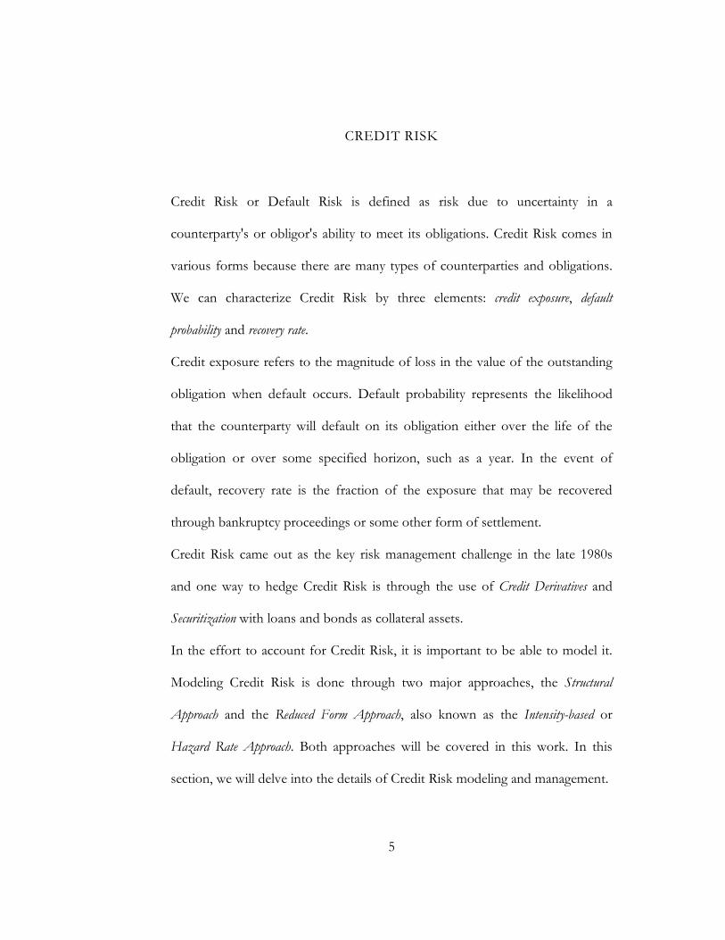
CREDIT RISK

Credit Risk or Default Risk is defined as risk due to uncertainty in a

counterparty's or obligor's ability to meet its obligations. Credit Risk comes in

various forms because there are many types of counterparties and obligations.

We can characterize Credit Risk by three elements: credit exposure, default

probability and recovery rate.

Credit exposure refers to the magnitude of loss in the value of the outstanding

obligation when default occurs. Default probability represents the likelihood

that the counterparty will default on its obligation either over the life of the

obligation or over some specified horizon, such as a year. In the event of

default, recovery rate is the fraction of the exposure that may be recovered

through bankruptcy proceedings or some other form of settlement.

Credit Risk came out as the key risk management challenge in the late 1980s

and one way to hedge Credit Risk is through the use of Credit Derivatives and

Securitization with loans and bonds as collateral assets.

In the effort to account for Credit Risk, it is important to be able to model it.

Modeling Credit Risk is done through two major approaches, the Structural

Approach and the Reduced Form Approach, also known as the Intensity-based or

Hazard Rate Approach. Both approaches will be covered in this work. In this

section, we will delve into the details of Credit Risk modeling and management.

6

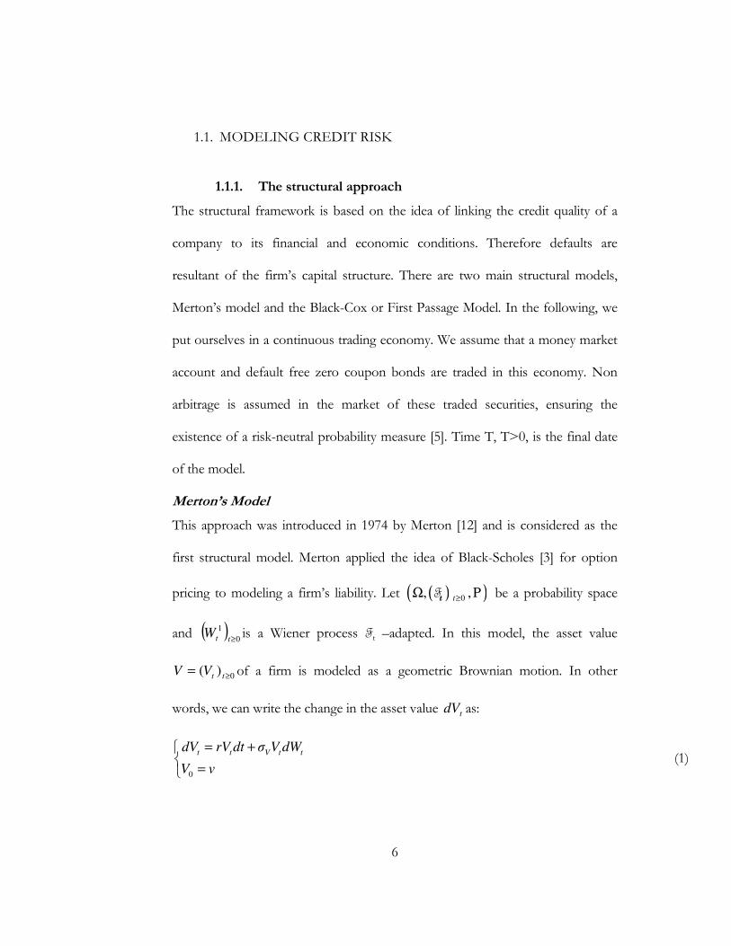
1.1. MODELING CREDIT RISK

1.1.1. The structural approach

The structural framework is based on the idea of linking the credit quality of a

company to its financial and economic conditions. Therefore defaults are

resultant of the firm’s capital structure. There are two main structural models,

Merton’s model and the Black-Cox or First Passage Model. In the following, we

put ourselves in a continuous trading economy. We assume that a money market

account and default free zero coupon bonds are traded in this economy. Non

arbitrage is assumed in the market of these traded securities, ensuring the

existence of a risk-neutral probability measure [5]. Time T, T>0, is the final date

of the model.

Merton’s Model

This approach was introduced in 1974 by Merton [12] and is considered as the

first structural model. Merton applied the idea of Black-Scholes [3] for option

pricing to modeling a firm’s liability. Let ( )( )0, ,t≥Ω PFt

be a probability space

and ( )0

1

≥ttW is a Wiener process Ft –adapted. In this model, the asset value

0)( ≥= ttVV of a firm is modeled as a geometric Brownian motion. In other

words, we can write the change in the asset value tdV as:

0

t t V t tdV rV dt σ V dW

V v

= +

= (1)

7

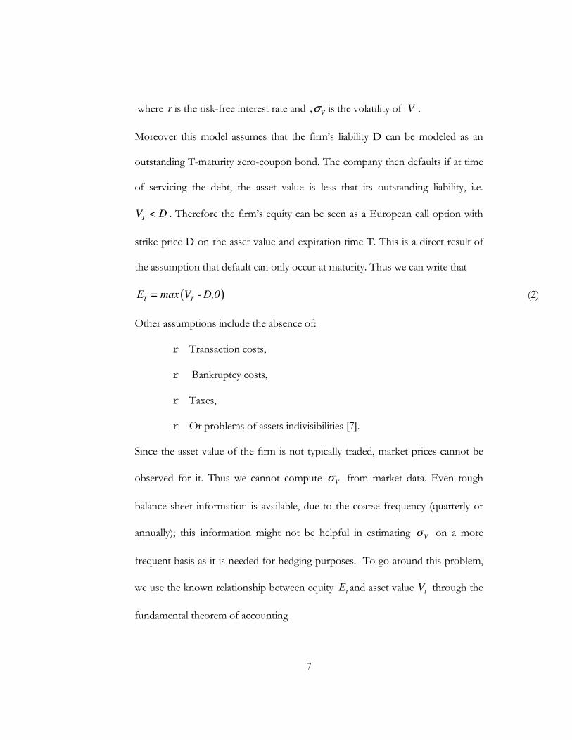
where r is the risk-free interest rate and Vσ, is the volatility of V .

Moreover this model assumes that the firm’s liability D can be modeled as an

outstanding T-maturity zero-coupon bond. The company then defaults if at time

of servicing the debt, the asset value is less that its outstanding liability, i.e.

TV < D . Therefore the firm’s equity can be seen as a European call option with

strike price D on the asset value and expiration time T. This is a direct result of

the assumption that default can only occur at maturity. Thus we can write that

( )T TE = max V - D,0 (2)

Other assumptions include the absence of:

r Transaction costs,

r Bankruptcy costs,

r Taxes,

r Or problems of assets indivisibilities [7].

Since the asset value of the firm is not typically traded, market prices cannot be

observed for it. Thus we cannot compute Vσ from market data. Even tough

balance sheet information is available, due to the coarse frequency (quarterly or

annually); this information might not be helpful in estimating Vσ on a more

frequent basis as it is needed for hedging purposes. To go around this problem,

we use the known relationship between equity tE and asset value tV through the

fundamental theorem of accounting

8

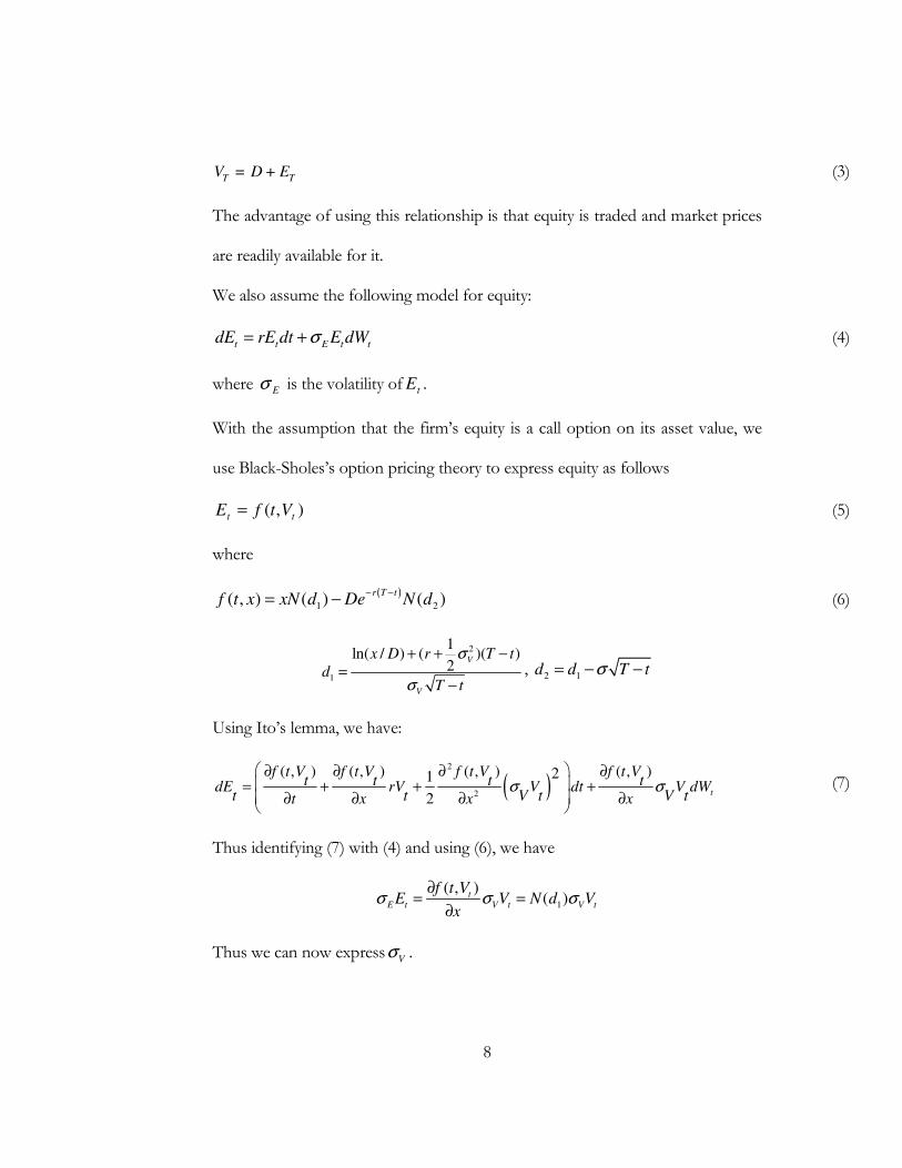
T TV = D + E (3)

The advantage of using this relationship is that equity is traded and market prices

are readily available for it.

We also assume the following model for equity:

t t E t tdE rE dt E dWσ= + (4)

where Eσ is the volatility of tE .

With the assumption that the firm’s equity is a call option on its asset value, we

use Black-Sholes’s option pricing theory to express equity as follows

),( tt VtfE = (5)

where

( )1 2( , ) ( ) ( )

r T tf t x xN d De N d

− −= − (6)

2

1

1ln( / ) ( )( )

2V

V

x D r T t

dT t

σ

σ

+ + −=

−,

2 1d d T tσ= − −

Using Ito’s lemma, we have:

( )2

2

( , ) ( , ) ( , ) ( , )21

2t

f t V f t V f t V f t Vt t t tdE rV V dt V dW

t t V t V tt x x xσ σ

∂ ∂ ∂ ∂ = + + + ∂ ∂ ∂ ∂

(7)

Thus identifying (7) with (4) and using (6), we have

1

( , )( )t

E t V t V t

f t VE V N d V

xσ σ σ

∂= =

∂

Thus we can now expressV

σ .

9

( )E t

V

d t

E

N d V

σσ = (8)

Where

2

21

( )2

zxN x e dz

π

−

= ∫−∞

is the cumulative distribution function of the

standard normal random variable.

We then use tE^ the observed market price of equity, and

^

tV obtained through

averaging a time series of asset values from the available balance sheets to

estimate V

σ as

^^

^ ^

1( )

E tV

t

E

N d V

σσ ≈ (9)

Where

^^2

^

1 ^

1ln( / ) ( )( )

2t V

V

V D r T t

d

T t

σ

σ

+ + −=

−

.

Then, we can solve numerically for ^

Vσ (10)

The only other parameter needed in the approximation is the liability D. To

estimate D, the face value of the zero-coupon T-maturity bond used to model the

firm’s liability, Sundaram [21] points out that “default tends to occur in practice

when the market value of the firm’s assets drops below a critical point that

typically lies below the book value of all liabilities, but above the book value of

10

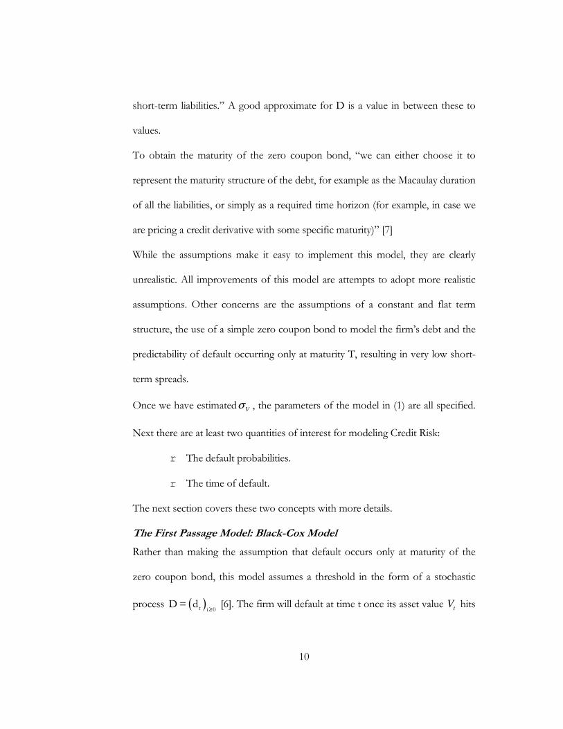
short-term liabilities.” A good approximate for D is a value in between these to

values.

To obtain the maturity of the zero coupon bond, “we can either choose it to

represent the maturity structure of the debt, for example as the Macaulay duration

of all the liabilities, or simply as a required time horizon (for example, in case we

are pricing a credit derivative with some specific maturity)” [7]

While the assumptions make it easy to implement this model, they are clearly

unrealistic. All improvements of this model are attempts to adopt more realistic

assumptions. Other concerns are the assumptions of a constant and flat term

structure, the use of a simple zero coupon bond to model the firm’s debt and the

predictability of default occurring only at maturity T, resulting in very low short-

term spreads.

Once we have estimated Vσ , the parameters of the model in (1) are all specified.

Next there are at least two quantities of interest for modeling Credit Risk:

r The default probabilities.

r The time of default.

The next section covers these two concepts with more details.

The First Passage Model: Black-Cox Model

Rather than making the assumption that default occurs only at maturity of the

zero coupon bond, this model assumes a threshold in the form of a stochastic

process ( )≥t t 0

D= d [6]. The firm will default at time t once its asset value t

V hits

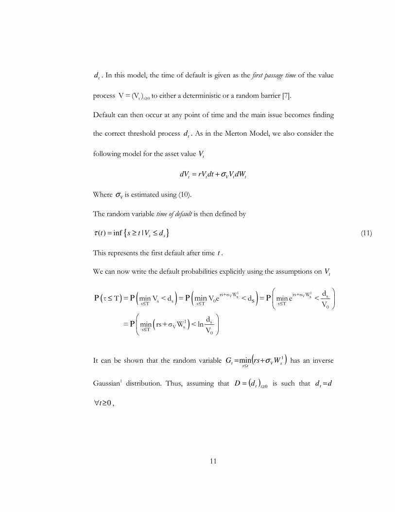
11

td . In this model, the time of default is given as the first passage time of the value

process ≥t t 0V =(V ) to either a deterministic or a random barrier [7].

Default can then occur at any point of time and the main issue becomes finding

the correct threshold process t

d . As in the Merton Model, we also consider the

following model for the asset value t

V

t t V t tdV rV dt V dWσ= +

Where V

σ is estimated using (10).

The random variable time of default is then defined by

( ) inf | s st s t V dτ = ≥ ≤ (11)

This represents the first default after time t .

We can now write the default probabilities explicitly using the assumptions on tV

( ) ( ) ( )

( )

≤ ≤ ≤

≤

≤

P P P P

P

1 1V Vrs+σ W rs+σ W ss s

s s 0s T s T s T

0

1 sV s

s T0

dτ T = min V < d = V e < d = min e <s

V

d= min rs+σ W < ln

V

min

It can be shown that the random variable ( )1min sVts

t WrsG σ+=≤

has an inverse

Gaussian1 distribution. Thus, assuming that ( )0≥

=ttdD is such that dd t =

0≥∀t ,

12

( )

≤

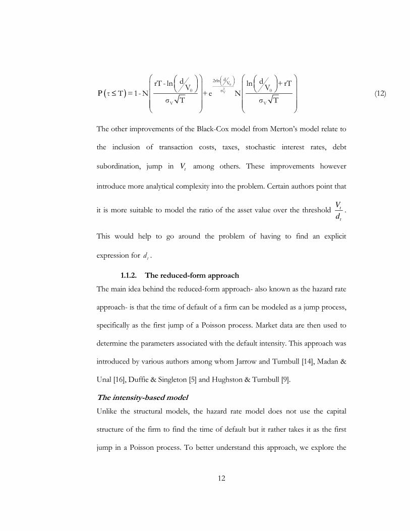
P

0

2V

d2rlnV

0 σ 0

V V

d drT - ln ln + rTV V

τ T =1-N +e Nσ T σ T

(12)

The other improvements of the Black-Cox model from Merton’s model relate to

the inclusion of transaction costs, taxes, stochastic interest rates, debt

subordination, jump in t

V among others. These improvements however

introduce more analytical complexity into the problem. Certain authors point that

it is more suitable to model the ratio of the asset value over the threshold t

t

V

d.

This would help to go around the problem of having to find an explicit

expression for td .

1.1.2. The reduced-form approach

The main idea behind the reduced-form approach- also known as the hazard rate

approach- is that the time of default of a firm can be modeled as a jump process,

specifically as the first jump of a Poisson process. Market data are then used to

determine the parameters associated with the default intensity. This approach was

introduced by various authors among whom Jarrow and Turnbull [14], Madan &

Unal [16], Duffie & Singleton [5] and Hughston & Turnbull [9].

The intensity-based model

Unlike the structural models, the hazard rate model does not use the capital

structure of the firm to find the time of default but it rather takes it as the first

jump in a Poisson process. To better understand this approach, we explore the

13

“time to default” process. As in section 1.1.1, we let ( )( )P,, 0≥Ω ttF be a

probability space and let τ denote the time to default or the waiting time for the

happening of default. Let )(tS be the probability of survival after time t. In other

words,

PS(t)= (τ > t) (13)

Thus

( ) 1 ( ) ( )F t S t tτ= − = ≤P (14)

is the probability of default before or at time t.

Since we assume no default at time 0, we have 1)0( =S .

The question then is to find an appropriate distribution that can be used to model

the default probabilities.

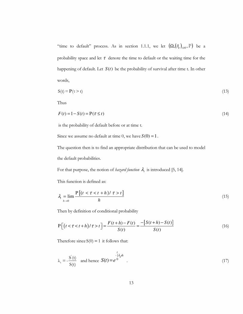
For that purpose, the notion of hazard function tλ is introduced [5, 14].

This function is defined as:

( )[ ]τ τλ

→

< < + >=

0

/limt

h

t t h t

h

P (15)

Then by definition of conditional probability

( )[ ]( ) ( )( ) ( )

/( ) ( )

S t h S tF t h F tt t h t

S t S tτ τ

− + −+ −< < + > = = P (16)

Therefore since 1S(0) = it follows that:

'

t

S (t)λ = -

S(t) and hence

-

0( )

tds

s

S t eλ∫

= . (17)

14

Observe that if we assume t

λ to be constant and equal toλ , we have

−= λtS(t) e (18)

Therefore, under these assumptions, τ has an exponential distribution with

parameter λ>0.

Knowing this, it seems plausible [2] to assume that there is a sequence ( ) 0≥iτ of

independent random variables, exponentially distributed with parameter λ>0 such

that: 1τ is the time to the 1st default, 2τ is the time between the 1st and 2nd

default,…, nτ is the time between the (n-1)th and nth defaults and so on.

The sequence ( )0≥iiτ represents an infinite sequence of random variables on the

probability space. The variable 1 2 ...n n

τ τ τΜ = + + + characterizes the time to the

nth default with 0 0Μ = . With the assumptions that two defaults cannot happen

simultaneously and that only a finite number of defaults can happen in each

interval time, ( )0n n≥

Μ is an increasing sequence that converges to infinity. Thus

0 1 20 ( ) ( ) ( ) ...ω ω ω= Μ < Μ < Μ < and sup ( )n

n

ωΜ = ∞ .

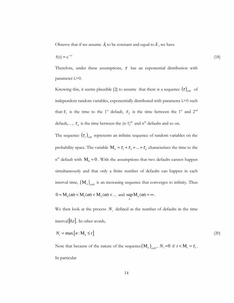
We then look at the process tN defined as the number of defaults in the time

interval [ ]t,0 . In other words,

[ ]max :t nN n t= Μ ≤ (20)

Note that because of the nature of the sequence ( )0n n≥

Μ , 0=tN if 1 1t τ< Μ = .

In particular

15

00 =N .

We deduce that the number of defaults in the time interval ( ]ts, is the

increment st NN − .

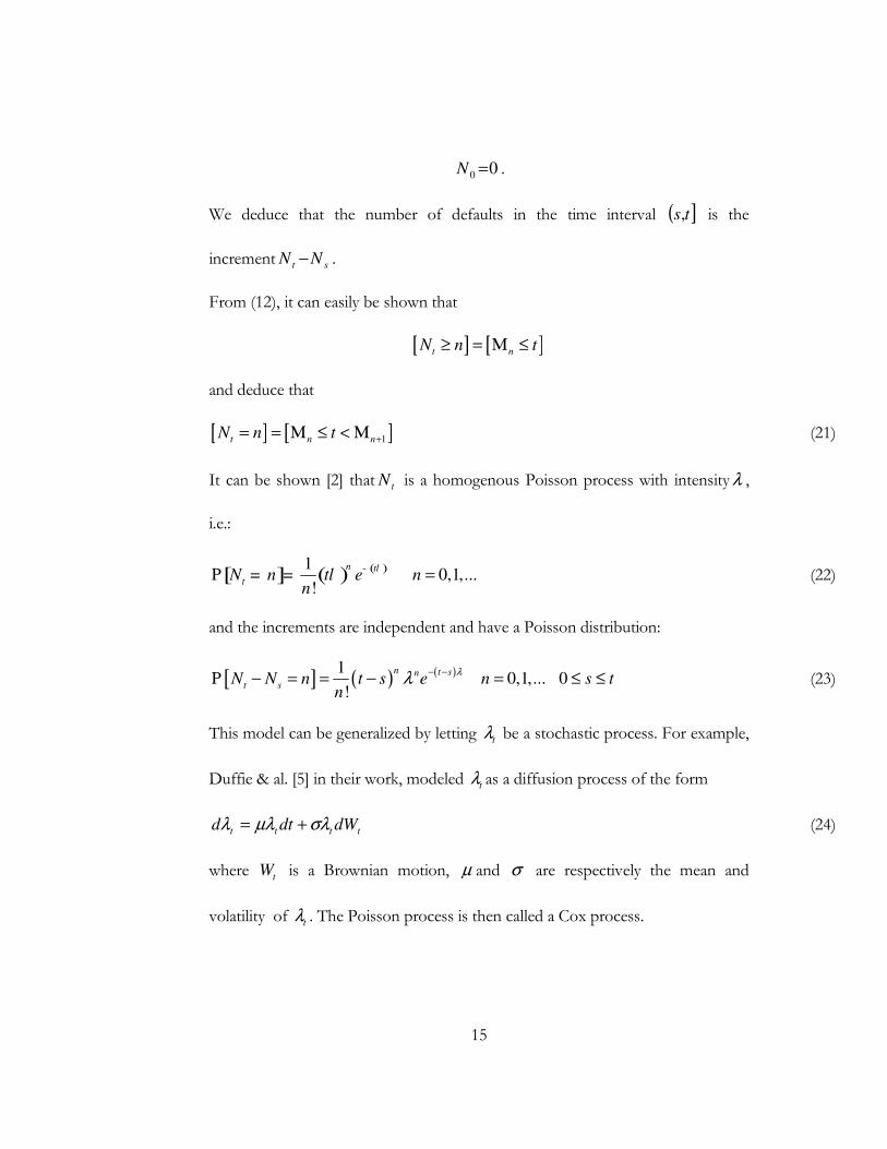
From (12), it can easily be shown that

[ ] [ ]t nN n t≥ = Μ ≤

and deduce that

[ ] [ ]1t n nN n t += = Μ ≤ < Μ (21)

It can be shown [2] that tN is a homogenous Poisson process with intensityλ ,

i.e.:

[ ] ( ) ( )1

!

n t

tN n t e

n

ll

-= =P 0,1,...n = (22)

and the increments are independent and have a Poisson distribution:

[ ] ( ) ( )1

!

n t sn

t sN N n t s e

n

λλ − −− = = −P 0,1,...n = 0 s t≤ ≤ (23)

This model can be generalized by letting t

λ be a stochastic process. For example,

Duffie & al. [5] in their work, modeled t

λ as a diffusion process of the form

tttt dWdtd σλµλλ += (24)

where t

W is a Brownian motion, µ and σ are respectively the mean and

volatility of t

λ . The Poisson process is then called a Cox process.

16

1.2. MANAGING CREDIT RISK

Let’s introduce some common terms that will be used in the remainder of this

thesis.

Credit Derivative is a derivative instrument designed to transfer credit risk from one

party to another. A Credit Event is an event such as a debt default or bankruptcy

that will affect the payoff on a credit derivative A Reference Asset is an asset, such

as a corporate or sovereign debt instrument that underlies a credit derivative. A

Reference Entity is the issuer of a Reference Asset. A Notional Amount is the amount

of the Reference Asset par value to which a contract applies. The Par value of a

bond is usually the amount the issuing company promises to pay at the maturity

date of the bond. In the most general sense, a spread is the difference between two

similar measures. In the credit derivatives market, spread is computed using bid

and offer quotes from dealers. A basis point (bps) is a unit equal to 1/100th of 1%.

In this paper, it is used as a unit for the spread.

1.2.1. Credit Derivatives

Credit Derivatives represent one of the most important innovations of the

financial industry in the last 15 years [1]. They allow isolating and trading the

Reference Entity’s credit risk through a partial or total transfer. They come in

various types and flavors, the most common being:

r Collateralized Debt Obligations (CDO)

r Credit Default Swaps (CDS)

17

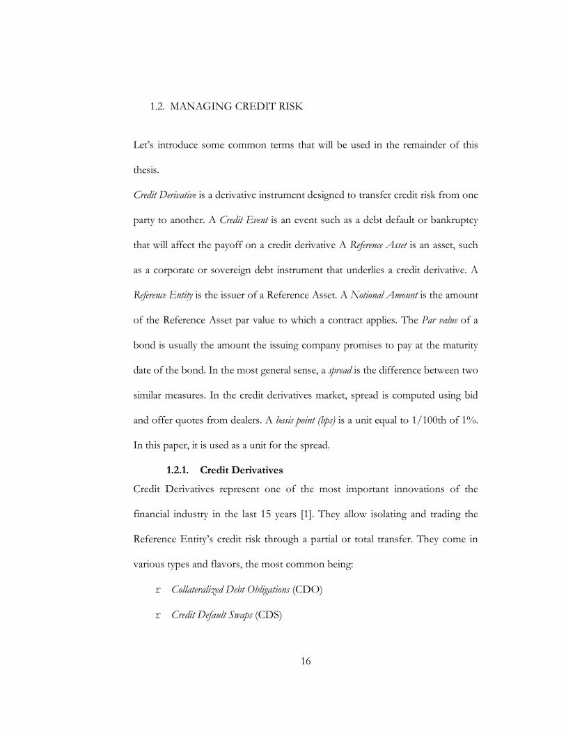
Other types of credit derivatives include Total Return Swaps and Credit-Linked

Notes. While the latter are still frequently used and described in the literature [10],

this project will focus on CDS and CDO. The figure below illustrates the Credit

Derivatives market as of 2003.

Figure 1Credit Derivative market breakdown by instrument type

Collateralized Debt Obligations (CDO)

CDO ([10]) are investment-grade securities backed by a pool of bonds, loans and

other assets. CDO are also referred to as portfolio correlation products. They represent

a way of packaging Credit Risk. Four classes called tranches are created from a

portfolio of corporate bonds or bank loans or asset-backed securities. The first

tranche owns 5% of the principal of the portfolio and bears the first 5% default

losses. 10% of the principal belongs to the second tranche which also takes the

next 10% default losses. The third tranche has 10% of the principal and takes in

the next 10% default losses. Finally the fourth tranche owns the remaining 75%

of the principal and absorbs the residual losses.

18

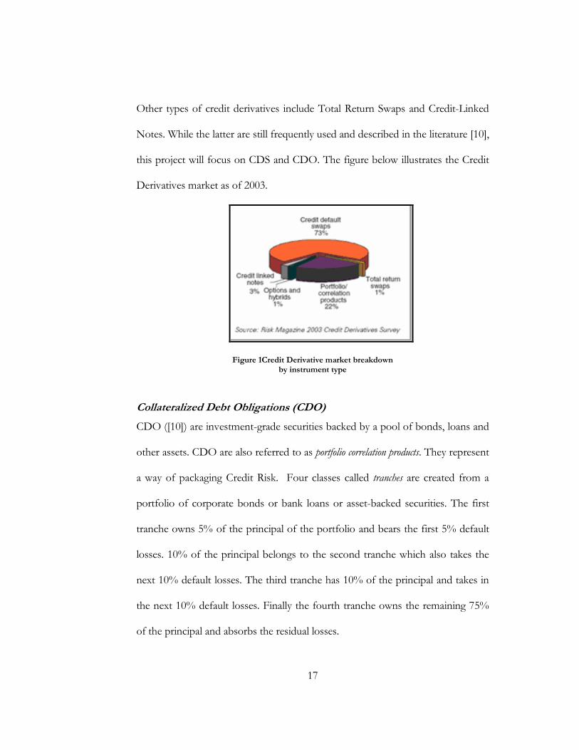
The figure below illustrates a CDO.

Tranche 4 is usually called the super senior tranche, tranche 3, the senior tranche,

tranche 2, the mezzanine and tranche 1, the subordinate tranche or “toxic waste”.

The structure of the CDO is supported by a rating given by the ratings agencies

such as Moody’s, S&P, and Fitch. Although these ratings might vary slightly

among these agencies, the highest rates, equivalent to almost default-free are the

AAA or Aaa, and the lowest, also called “junk” are rated C, Ca or D.

Tranche 4 is usually rated AAA by S&P and Aaa by Moody’s because almost no

default risk is associated with that tranche. Despite the existence of default risk in

Tranche 3, it is still lower than that of the entire underlying portfolio. Unlike

tranche 3, tranche 2 is probably more risky than the portfolio. Tranche 1 can be

very risky. A 5% loss in the portfolio will translate in a 100% loss in that tranche.

Bond 1 Bond 2 Bond 3

.

.

.

.

.

.

.

.

. Bond n

Average yield

y%

Trust

Tranche 1 1st 5% loss Yield=35%

Tranche 2 2nd 10% loss Yield=15%

Tranche 3 3rd 10% loss Yield=7.5%

Tranche 4 Residual loss Yield=8%

19

That is the reason why this tranche is usually retained by the creator of the CDO,

given the high risk associated with it. CDO allow creating high-quality debt with

average quality. An important issue is the correlation between bonds in the

portfolio, given that the risk to which the mezzanine, senior and super senior

tranches are exposed depend on that. Recently, copula models, which are statistical

models, are being used to incorporate the correlation between the elements of a

CDO.

Credit Default Swaps (CDS)

CDS ([1, 19]) are the simplest type of credit derivatives and act as a form of

insurance. If the reference asset is one bond of a single firm, they are called

single-name CDS. If the Reference Asst is a portfolio of bonds, then we talk

about multi-name CDS. There are also CDS backed by an index such as the Dow

Jones index. In that case, they are called CDX.

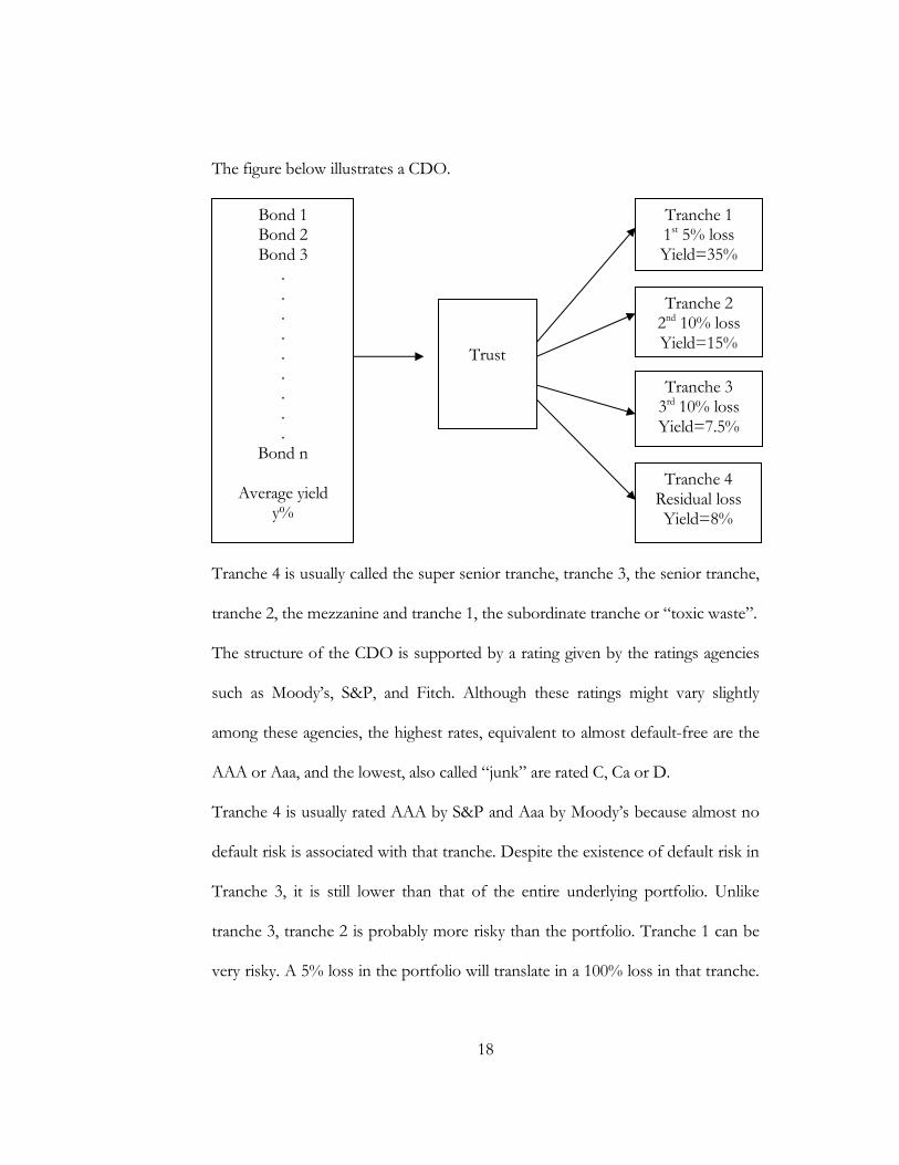
In a CDS contract, one party (the protection buyer or Credit Risk seller) is

protected from a Reference Entity default through the payment of a regular

Premium to the other party (the protection seller or Credit Risk buyer), entitling

the former a payment of any non recoverable amount in the event of the

Reference Entity default. This process is illustrated below:

20

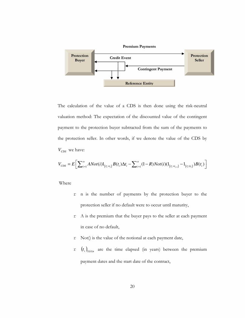
The calculation of the value of a CDS is then done using the risk-neutral

valuation method: The expectation of the discounted value of the contingent

payment to the protection buyer subtracted from the sum of the payments to

the protection seller. In other words, if we denote the value of the CDS by

CDSV we have:

11 1( )1 ( ) (1 ) ( )(1 1 ) ( )

i i i i i i

n n

CDS i i it t ti iV E ANot i B t t R Not i B t

τ τ τ−> > ≤= = = ∆ − − − ∑ ∑

Where

r n is the number of payments by the protection buyer to the

protection seller if no default were to occur until maturity,

r A is the premium that the buyer pays to the seller at each payment

in case of no default,

r Not() is the value of the notional at each payment date,

r ( )niit ≤≤1 are the time elapsed (in years) between the premium

payment dates and the start date of the contract,

PPrrootteeccttiioonn BBuuyyeerr

PPrrootteeccttiioonn

SSeelllleerr

PPrreemmiiuumm PPaayymmeennttss

RReeffeerreennccee EEnnttiittyy

CCrreeddiitt EEvveenntt

CCoonnttiinnggeenntt PPaayymmeenntt

21

r ( )nii ≤≤1

τ are as defined in Section 1.1.2,

r ( )iB t is the discounting factor at it ,

r R is the recovery rate of the Reference Asset in case of default,

r And [ ]E is the expectation under the probabilityΠ.

Therefore under the assumptions that default events, recovery rates and interest

rates are mutually independent we obtain:

( ) ( ) ( )∑ ∑= = − −−−∆=n

i

n

i iiiiiiCDS tBtStSiNotRttBtSiANotV1 1 1 )()(()1()()( (25)

At origination, under the risk neutral valuation framework, we should have

0=CDSV

More details about CDS will be provided in Chapter 2.

1.2.2. Synthetic Securitization

The idea behind synthetic securitization is among others, to allow credit

protection, capital relief and exposure to an asset without having the obligation

to retain ownership of the asset. For example a bank can transfer the Credit

Risk associated with a portfolio of BBB-rated (medium credit quality) corporate

loans to a bankruptcy remote special purpose financing vehicle without actually

transferring the underlying loans. The special purpose vehicle (SPV) can then

issue securities whose interest and principal payments are provided by cash

flows coming from the loans. The SPV then creates a portfolio of single-name

CDS on each the security type and buys protection synthetically for the CDO,

therefore replicating the CDO synthetically. In this way, the bank is able to

22

avoid sensitive client relationship issues arising from loan transfer notification

requirements, loan assignment provisions, and loan participation restrictions. It

is also able to maintain client confidentiality.

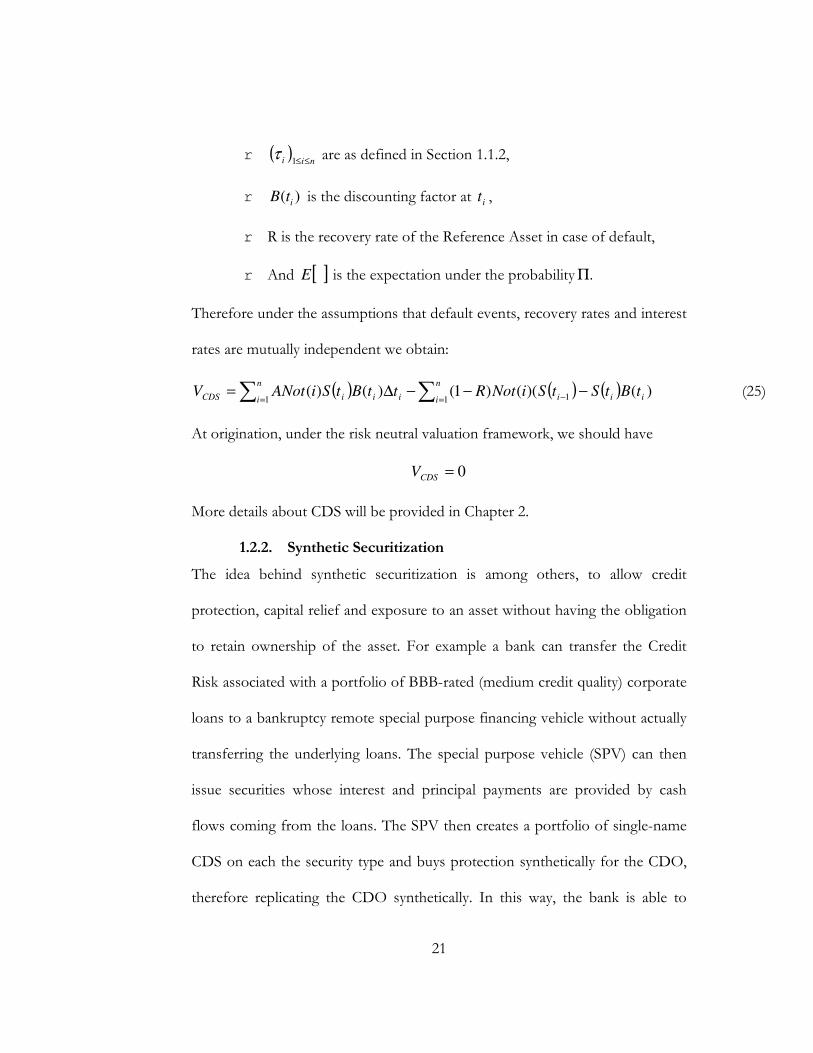
Almost inexistent in 2001, the synthetic products market has grown quickly as

illustrated by the figure below (reference).

Figure 2 Breakdown of the CDS market in 2001 and………………2003

There are many types of synthetic credit derivatives such as Synthetic CDO

(SCDO), Single Tranche CDO (STCDO).

Synthetic CDO (SCDO)

Synthetic CDO are artificial CDO that are backed by a pool of credit derivatives

such as CDS, forwards, and options. SCDO achieve exposure to the pool of

assets underlying these derivatives by synthetically selling CDS. In such a CDS,

the SCDO receives a periodic payment from a counterparty that seeks protection

against the default of a referenced asset. A special purpose vehicle is used to

structure a SCDO and it can issue floating or fixed rate obligations tranched in a

23

variety of ways with respect to seniority and payment. SCDO obligations can

have special features customized or tailor-made to investor requirements.

Single-Tranche Synthetic CDO (STSCDO)

A single-tranche CDO is one where the sponsor sells only one tranche from the

capital structure of a synthetic CDO. It is also known as mezzanine-only CDO,

instant CDO (iCDO), custom tailored CDO tranches and bespoke (meaning

custom tailored) CDO tranches, STCDO deals are based on synthetic CDO

technology. A bank arranger will create a customized tranche for an investor. The

investor chooses the initial portfolio – usually a portfolio of diversified corporate

reference credits. The portfolio may be static, or the investor may “lightly

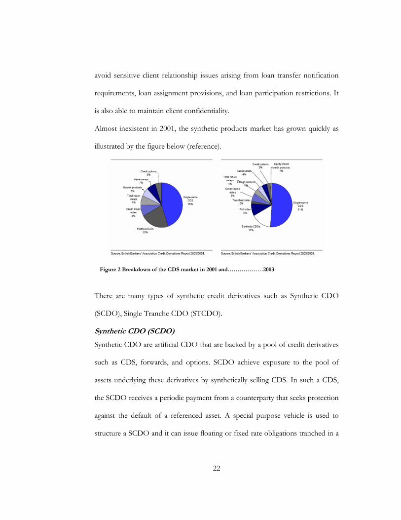
manage” the portfolio, usually at no extra cost. A tranche is defined by its

attachment point and its detachment point. These two elements characterize its

position in the CDO structure as illustrated in the figure below.

Figure 3Tranches on CDX or more generally Single Tranche CDO

24

CREDIT DEFAULT SWAPS

A CDS is a form of OTC credit derivative security, which can be regarded as

default insurance on reference assets such as bonds or loans. CDS are one of the

most innovative financial instruments in the last decade and are expanding very

rapidly and successfully. According to the November 2005 report of the Bank of

International Settlements (BIS) on the Global OTC Derivatives Market at end-

June 2005 “Notional Amounts outstanding of credit default swaps rose by 60%

during the first half of 2005 to $10.2 trillion, weathering the sell-off in credit

markets triggered by downgrades in the US auto industry in March.3 Growth was

particularly strong in multi-name contracts, whose Notional Amount more than

doubled to $2.9 trillion, single-name CDS increased by 43% to $7.3 trillion. The

vast majority of contracts have maturities between one and five years.” [22]

CDS is a sophisticated form of a traditional financial guarantee, with the

difference that it needs not be limited to compensation upon an actual default but

might even cover events such as downgrading, apprehended default etc.

CDS covers only the Credit Risk inherent in the asset, while risks on account of

other factors such as interest rate movements remain with the originator.

CDS are used as a way of hedging a specific exposure to a specific asset or as a

mean to gain exposure to a specific asset.

25

Two parties are involved in a CDS, protection buyers or risk sellers and

protection sellers or risk buyers. Protection buyers express their negative view of

the performance of the specific asset by seeking insurance for a default event.

Protection sellers on the other hand gain exposure to the specific asset.

The protection buyer, hereafter referred to as the buyer agrees to pay a Premium

to the protection seller until a credit event occurs or maturity is attained. The

protection seller, hereafter referred to as the seller, agrees to pay the contingent

value to the buyer in case a default event occurs.

At the time of definition, a CDS contract comes with various specifications.

Apart from the Premium, the Maturity Date and the Notional Amount, the other

ingredients to a CDS contract:

r Specification of the credit events

r Type of settlement ( physical or cash)

r Payment frequency

r Business day convention

r Discounting factor

r Effective date

According to an article that appeared on Bloomberg News on November 18th

2005, “GM was among the five companies most frequently included in credit-

derivatives contracts in 2004, along with Ford Motor Co., France Telecom SA,

DaimlerChrysler AG and Deutsche Telekom AG, Fitch said. Investors bought

26

more contracts protecting payments from Korea, Italy and Russia than any other

governments.”

We observe a wide range of participants in the credit-derivatives market. In the

same article cited above, it is said that “The survey of 120 banks and financial

institutions showed that banks are typically net buyers of debt insurance because

they can use default swaps to reduce the risk of corporate loans. Banks used

credit derivatives to transfer a record $427 billion of credit risk from their balance

sheets to other counterparties in 2004, up from $260 billion a year earlier, Fitch

said.” According to a survey from the BBA, “Banks, security houses, and hedge

funds dominate the protection-buyers market, with banks representing about 50

percent of the demand. On the protection-sellers side, banks and insurance

companies dominate [23].

We can distinguish two types of CDS, corporate CDS and Asset-Backed CDS.

2.1. CORPORATE CDS

The Reference Asset, also know as Reference Obligation, in this case is a

corporate bond and the Reference Entity is a firm. One of the distinctive features

of corporate CDS is that the contract terminates at the first credit event or when

the bond matures, whichever comes first.

The buyer agrees to pay a Premium to the seller until the underlying Reference

Entity defaults or the bond matures, whichever comes first. The CDS Premium is

27

typically quoted in basis points per $100 of the Notional Amount of the reference

asset. In return the seller makes the engagement to buy the defaulted bond at par

value from the buyer.

In the case of a corporate CDS, the guidelines for credit events set by ISDA (the

International Swaps and Dealers Association) are:

r Failure to Pay,

r Loss event,

r Bankruptcy,

r And downgrading.

The type of settlement can be:

r Physical, in which case the seller buys the reference asset at par

r Cash, entitling the buyer the reimbursement of the defaulted amount.

In [10] we can see the following example: suppose two parties enter into a five-

year CDS on March 1, 2002. Assume that the notional principal is $100 million

and the buyer agrees to pay 90 bps annually for protection against default by the

reference entity. If the Reference Entity does not default (i.e. there is no default

event), the buyer receives no payoff and pays $900,000 on March 1 of the years

2003, 2004, 2005, 2006 and 2007. If there is a credit event, a substantial payoff is

likely.

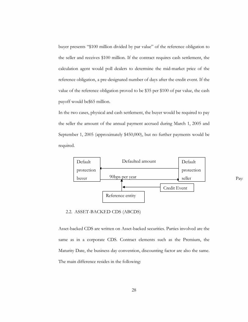
Suppose the buyer notifies the seller of a credit event on September 1, 2005

(halfway through the 4th year). If the contract specifies physical settlement, the

28

buyer presents “$100 million divided by par value” of the reference obligation to

the seller and receives $100 million. If the contract requires cash settlement, the

calculation agent would poll dealers to determine the mid-market price of the

reference obligation, a pre-designated number of days after the credit event. If the

value of the reference obligation proved to be $35 per $100 of par value, the cash

payoff would be$65 million.

In the two cases, physical and cash settlement, the buyer would be required to pay

the seller the amount of the annual payment accrued during March 1, 2005 and

September 1, 2005 (approximately $450,000), but no further payments would be

required.

Payment if default by reference entity

2.2. ASSET-BACKED CDS (ABCDS)

Asset-backed CDS are written on Asset-backed securities. Parties involved are the

same as in a corporate CDS. Contract elements such as the Premium, the

Maturity Date, the business day convention, discounting factor are also the same.

The main difference resides in the following:

90bps per year

Default

protection

buyer

Default

protection

seller

Reference entity

Defaulted amount

Credit Event

29

The ABCDS is a PAYGO contract; defaulted amounts are paid and reimbursed

as they happen, therefore the Notional Amount is not constant and might

increase or decrease. The contract is not terminated at the first credit event but

when the Outstanding Notional Balance becomes null or at Maturity Date,

whichever comes first. Additional provisions are the payment by the buyer to the

seller of any reimbursed defaulted amount. Also credit events include Principal

Writedown (reduction), Failure to pay while Bankruptcy is no longer considered.

2.3. CDS AS RISK MANAGEMENT TOOL

CDS be used by commercial banks as well as portfolios managers to diversify

their credit portfolios, reduce their exposure to credit risk and trade credit risk.

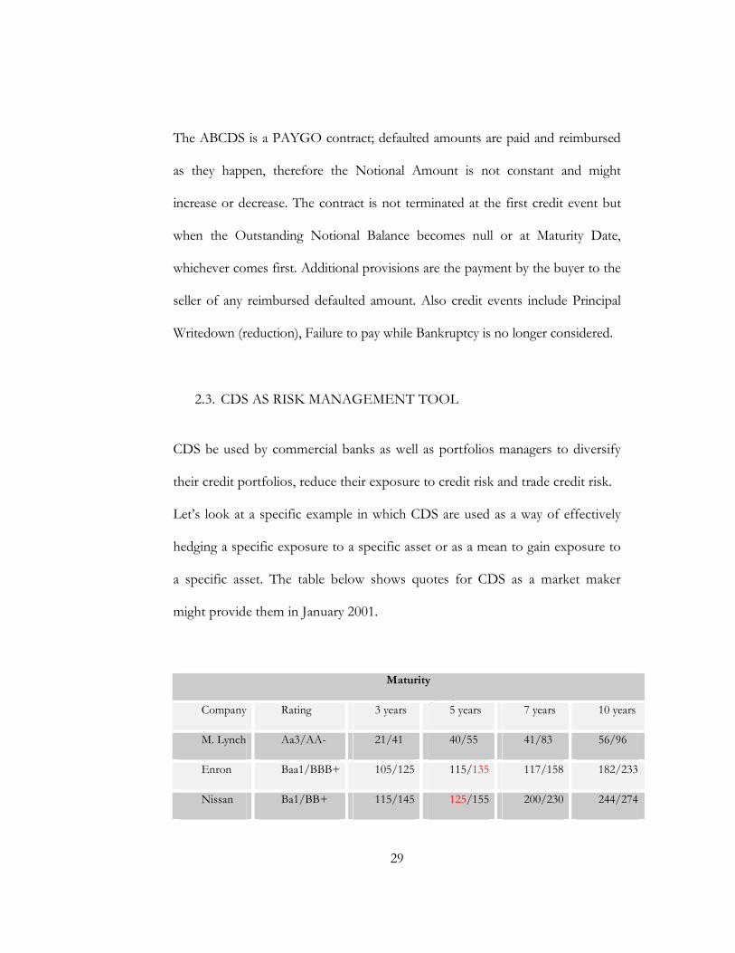
Let’s look at a specific example in which CDS are used as a way of effectively

hedging a specific exposure to a specific asset or as a mean to gain exposure to

a specific asset. The table below shows quotes for CDS as a market maker

might provide them in January 2001.

Maturity

Company Rating 3 years 5 years 7 years 10 years

M. Lynch Aa3/AA- 21/41 40/55 41/83 56/96

Enron Baa1/BBB+ 105/125 115/135 117/158 182/233

Nissan Ba1/BB+ 115/145 125/155 200/230 244/274

30

For the last 4 columns, the pair of numbers represents bid and offer quotes for

CDS with maturity 3, 5, 7 and 10 years. Suppose that a bank had several

hundreds million dollars of loans outstanding to Enron in January 2001 and was

concerned about its exposure. How can it use CDS to hedge its exposure to a

default by Enron? A possible hedging strategy would be to buy a $100 million

5-year CDS on Enron from the market maker in table 1 for 135bps or $1.35

million/year. This would shift to the market maker part of the bank’s Enron

credit exposure. Instead of shifting the credit exposure to the market maker, the

bank can also choose to exchange part of the exposure for an exposure to a

company in a totally different industry, say Nissan. The bank could sell a 5-year

$100 million CDS on Nissan for $1.25million/year at the same time as buying a

CDS on Enron. The net cost of this strategy would be 10bps or $100,000.

As it happens, Enron defaulted within 12 months of January 2001. Either

strategy would have worked out well!

2.4. ASSET-BACKED CDS VALUATION

In this section, we discuss the pricing of CDS in the reduced form framework.

In pricing CDS, there are two cases to consider: the primary market or at

origination and the secondary market or after origination. In the primary market,

31

we are pricing a CDS that has not been initiated yet while in the secondary

market, we are pricing an existing CDS. Both cases will be covered in this section.

Let’s consider a CDS contract with a constant notional )(tNot . We assume that

in the event of default, the seller will only pay the non- recoverable part

)()1( tNotR− of the notional. We also assume, for simplicity, the recovery rate R

to be constant. Let T be the length of the contract in years.

A CDS has two cash flow legs:

r The fixed leg or the Premium payments that the buyer pays to the seller

r And the floating leg or protection payments that the seller pays to the

buyer in the case of a credit event.

For simplicity we assume no counterparty credit risk. Then the pricing strategy is

as follows:

r In the primary market, risk neutral valuation is used to equate the present

value of these two legs and determine the fair price.

r In the secondary market, current CDS market prices are used to determine

the implied default probability and compute the value of the CDS contract.

Each case will be studied in details.

2.4.1. Pricing CDS in the primary market

Let ( )0≥kkm be defined as a sequence of a set of dates representing the possible

maturity dates of a CDS contract. km is usually chosen such that the length of

the contract follows the usual bond length agreement. In other words,

32

yearsm

yearm

yearm

2

1

21

3

2

1

=

=

=

Also let ( )1k

A≥k be a sequence representing the CDS market premiums

corresponding to the sequence ( )1k k

m≥. We know that each of these premiums

will depend on how the market perceives the credit risk associated with the

Reference Entity, i.e., the probability of default of the Reference Entity. kA is

paid periodically, for example every quarter, until the end of the contract or

until a certain credit event occurs for a corporate CDS or the Notional has been

entirely paid in the case of ABCDS or the contract reaches maturity.

Consider a CDS contract in which the Premium A is paid every quarter, at a set

of dates to which we associate a sequence ( )niit ≤≤1 , that represent the time

elapsed between the payment dates and the start date of the contract.

Thus Tttt n =<< ...21 .

We set 00 =t .

Given this definition, there will be some i

t such that ki mt = for Tmk ≤ .

Let ( )iF t be the probability that the Reference Entity will default by time

it (see equation (14)) and ( ) ( )1i iS t F t= − , the probability that the Reference

Entity will survive i

t .

33

One of the challenges for pricing ABCDS is that unlike with corporate CDS

where a credit event signifies the end of the CDS contract, a credit event merely

implies a contingent default payment if the notional is not exhausted. Another

salient feature is that contingent payments are dependent on the type of credit

event. Thus to express the default leg, one needs to take into account the

various type of credit events and their related time of default, as well as the

likely correlation among them.

In this work, to simplify the model, we assume only one type of credit event, a

principal writedown, implying a reduction in the notional.

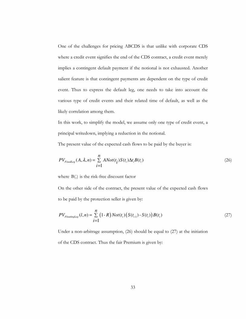
The present value of the expected cash flows to be paid by the buyer is:

( , , ) ( ) ( ) ( )1

i i iFixedLeg

nPV A n ANot t S t t B t

ii

λ = ∆∑=

(26)

where B(.) is the risk-free discount factor

On the other side of the contract, the present value of the expected cash flows

to be paid by the protection seller is given by:

( ) ( )-1( , ) 1- ( ) ( ) - ( ) ( )1

FloatingLeg i i i i

nPV l n R Not t S t S t B t

i

= ∑=

(27)

Under a non-arbitrage assumption, (26) should be equal to (27) at the initiation

of the CDS contract. Thus the fair Premium is given by:

34

( ) ( )−− −∑==

∆∑=

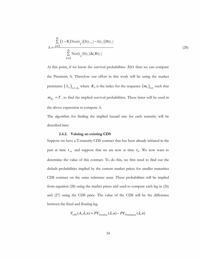
i 1 i i

i i i

n1 R Not(t ) S(t ) S(t ) B(t )

ii 1A

nNot(t )S(t ) t B(t )

ii 1

(28)

At this point, if we know the survival probabilities )(tS then we can compute

the Premium A. Therefore our effort in this work will be using the market

premiums ( )1.. Tk K=kA where TK is the index for the sequence ( )

1k km

≥ such that

TmTK = , to find the implied survival probabilities. These latter will be used in

the above expression to compute A.

The algorithm for finding the implied hazard rate for each maturity will be

described later.

2.4.2. Valuing an existing CDS

Suppose we have a T-maturity CDS contract that has been already initiated in the

past at time kt− and suppose that we are now at time 0t . We now want to

determine the value of this contract. To do this, we first need to find out the

default probabilities implied by the current market prices for smaller maturities

CDS contract on the same reference asset. These probabilities will be implied

from equation (28) using the market prices and used to compute each leg in (26)

and (27) using the CDS price. The value of the CDS will be the difference

between the fixed and floating leg.

( , , ) ( , ) ( , )CDS FixedLeg FloatingLeg

V A n PV n PV nλ λ λ= −

35

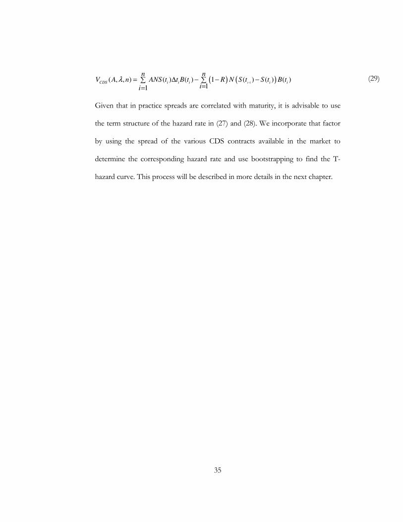
( ) ( )1( , , ) ( ) ( ) 1 ( ) ( ) ( )

11iCDS i i i i i

n nV A n ANS t t B t R N S t S t B t

ii

λ−

= ∆ − − −∑ ∑==

(29)

Given that in practice spreads are correlated with maturity, it is advisable to use

the term structure of the hazard rate in (27) and (28). We incorporate that factor

by using the spread of the various CDS contracts available in the market to

determine the corresponding hazard rate and use bootstrapping to find the T-

hazard curve. This process will be described in more details in the next chapter.

36

Data and Methods

In this work, we essentially used the risk-neutral valuation method within the

reduced form framework to value ABCDS in the secondary market. To account

for the dependence between spread and maturity, the bootstrapping method is

used find the term structure of the hazard rate.

C++ code was implemented to price ABCDS using the aforementioned

methods. The data source for this work is the INTEX database. The INTEX

cash flow engine was used to generate cash to use to test the methods and also

for comparing the effect of applying default at the tranche level and the

collaterals level.

3.1. THE HAZARD RATE METHOD USING BOOTSTRAPPING

Recall that from the hazard rate defined in section 1.1.2.1.

( ) /lim0

t t h t

t hh

τ τλ

< < + > =→

P,

We used this formula to derive an expression for the survival function in

terms of the hazard rate -

0

( )

tdss

S t e

λ∫

=

If we assume the hazard rate is constant, we have from equation (16):

37

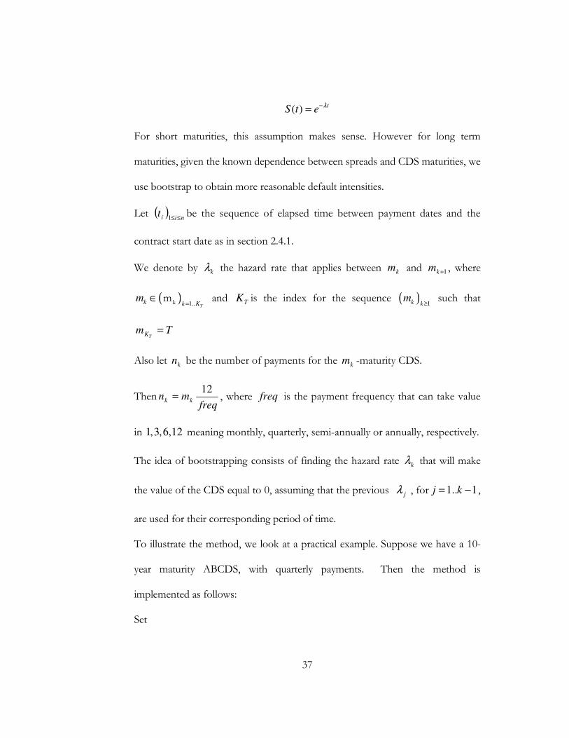
( ) tS t e λ−=

For short maturities, this assumption makes sense. However for long term

maturities, given the known dependence between spreads and CDS maturities, we

use bootstrap to obtain more reasonable default intensities.

Let ( )niit ≤≤1be the sequence of elapsed time between payment dates and the

contract start date as in section 2.4.1.

We denote by kλ the hazard rate that applies between km and 1+km , where

( )1.. T

k k Km

=∈ km and TK is the index for the sequence ( )

1k km

≥ such that

TmTK =

Also let kn be the number of payments for the km -maturity CDS.

Thenfreq

mn kk

12= , where freq is the payment frequency that can take value

in 1,3,6,12 meaning monthly, quarterly, semi-annually or annually, respectively.

The idea of bootstrapping consists of finding the hazard rate kλ that will make

the value of the CDS equal to 0, assuming that the previous jλ , for 1.. 1j k= − ,

are used for their corresponding period of time.

To illustrate the method, we look at a practical example. Suppose we have a 10-

year maturity ABCDS, with quarterly payments. Then the method is

implemented as follows:

Set

38

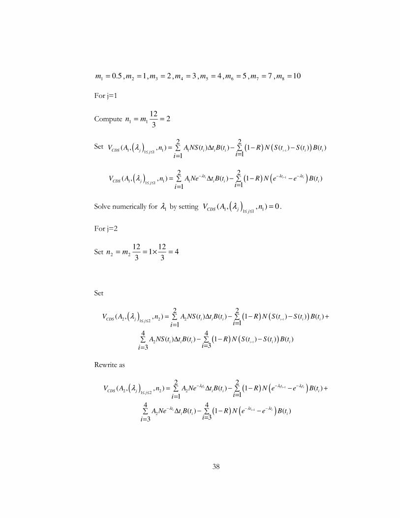
5.01 =m , 12 =m , 23 =m , 34 =m , 45 =m , 56 =m , 77 =m , 108 =m

For j=1

Compute 23

1211 == mn

Set ( ) ( ) ( )11 1 11 1

2 2( , , ) ( ) ( ) 1 ( ) ( ) ( )

11iCDS j i i i i ij

V A n A NS t t B t R N S t S t B tii

λ−≤ ≤

= ∆ − − −∑ ∑==

( ) ( ) ( )1

1 1 11 1

2 2( , , ) ( ) 1 ( )

11

i i it t t

CDS j i i ijV A n A Ne t B t R N e e B t

ii

λ λ λλ −− − −

≤ ≤= ∆ − − −∑ ∑

==

Solve numerically for 1λ by setting ( )1 11 1( , , ) 0CDS j j

V A nλ≤ ≤

= .

For j=2

Set 43

121

3

1222 =×== mn

Set

( ) ( ) ( )

( ) ( )

1

1

2 2 21 2

2

2 2( , , ) ( ) ( ) 1 ( ) ( ) ( )

11

4 4( ) ( ) 1 ( ) ( ) ( )

33

i

i

CDS j i i i i ij

i i i i i

V A n A NS t t B t R N S t S t B tii

A NS t t B t R N S t S t B tii

λ−

−

≤ ≤= ∆ − − − +∑ ∑

==

∆ − − −∑ ∑==

Rewrite as

( ) ( ) ( )

( ) ( )

1 1 1 1

1

2 2 21 2

2

2 2( , , ) ( ) 1 ( )

11

4 4( ) 1 ( )

33

i i i

i i i

t t t

CDS j i i ij

t t t

i i i

V A n A Ne t B t R N e e B tii

A Ne t B t R N e e B tii

λ λ λ

λ λ λ

λ −

−

− − −

≤ ≤

− − −

= ∆ − − − +∑ ∑==

∆ − − −∑ ∑==

39

Or

( ) ( ) ( ) ( )14 4

2 2 2 1 21 2 1 1 3 3

( , , ) ( , , ) ( ) 1 ( )i i it t t

CDS j CDS j i i ij j i i

V A n V A n A Ne t B t R N e e B tλ λ λλ λ −− − −

≤ ≤ ≤ ≤ = =

= + ∆ − − −∑ ∑

Then solve numerically for 2λ by setting ( )1 21 2( , , ) 0CDS j j

V A nλ≤ ≤

= .

Repeat the steps until 10K

m

We can generalize this process in the following:

Solve for 1λ by setting

( ) ( ) ( )1 1

11 1 11 1 1 1

( , , ) ( ) ( ) 1 ( ) ( ) ( ) 0i

n n

CDS j i i i i ij i i

V A n A NS t t B t R N S t S t B tλ−≤ ≤ = =

= ∆ − − − =∑ ∑

Then iteratively solve for kλ given 11 ,..., −kλλ in the following equation:

( )

( )

k 1

k

k 1 k 1

CDS k 1 1

n n1

k i i i i ii n i n

V (A , λ , n )

A Not(t ) ∆t B(t ) 1 R Not(t )( ) B(t ) 0k

i i k

t t ti i ie e e

λ λ λ

−

− −

≤ ≤ −

− − −−

= =

+

− − − =∑ ∑

For 2.. 1T

k K= −

So that at the end, the hazard rate function is a given as a step function of the

form:

=

≤≤

=

−

T

kk

k

Kk

mtm

t

,..,1

)(

1

λλ

40

3.2. RESULTS AND DISCUSSION

We now present a numerical example to illustrate the valuation process under

various scenarios. For that purpose, we consider a CDS contract with the

following specifications:

Start Date: 29/04/05

Next Pay Date: 25/05/05

Prev Pay Date: 25/04/05

Business Days: New York Banking

Discounting: 1 month LIBOR

Scenario: PPC 100/call

Notional: $7,500,000

Recovery: 40%

Premium (bps): 190

Curr Mkt Spread: 175

Maturity: 29/04/12

We consider 3 cases to evaluate the effect of the hazard rate curve on the value of

the CDS. In the first case, we assume one hazard rate, therefore ignoring the

dependence between spreads and maturities. In the second case we consider only

one market price available, i.e.TK

A , we assume a straight line hazard rate term

41

structure. A 3rd case is considered in which we assume the availability of a full

market spread structure, i.e. ( )1 T

k k KA

≤ ≤.

Case 1

Then using equation (20), we solve for the constant hazard rate λ and find that

0.032801778λ = and the swap value is $159,299 .00CDS

V =

While this might work for short-term maturities, it is clearly not realistic to use a

single point hazard rate to price CDS. It is well know that spreads are dependent

on maturities.

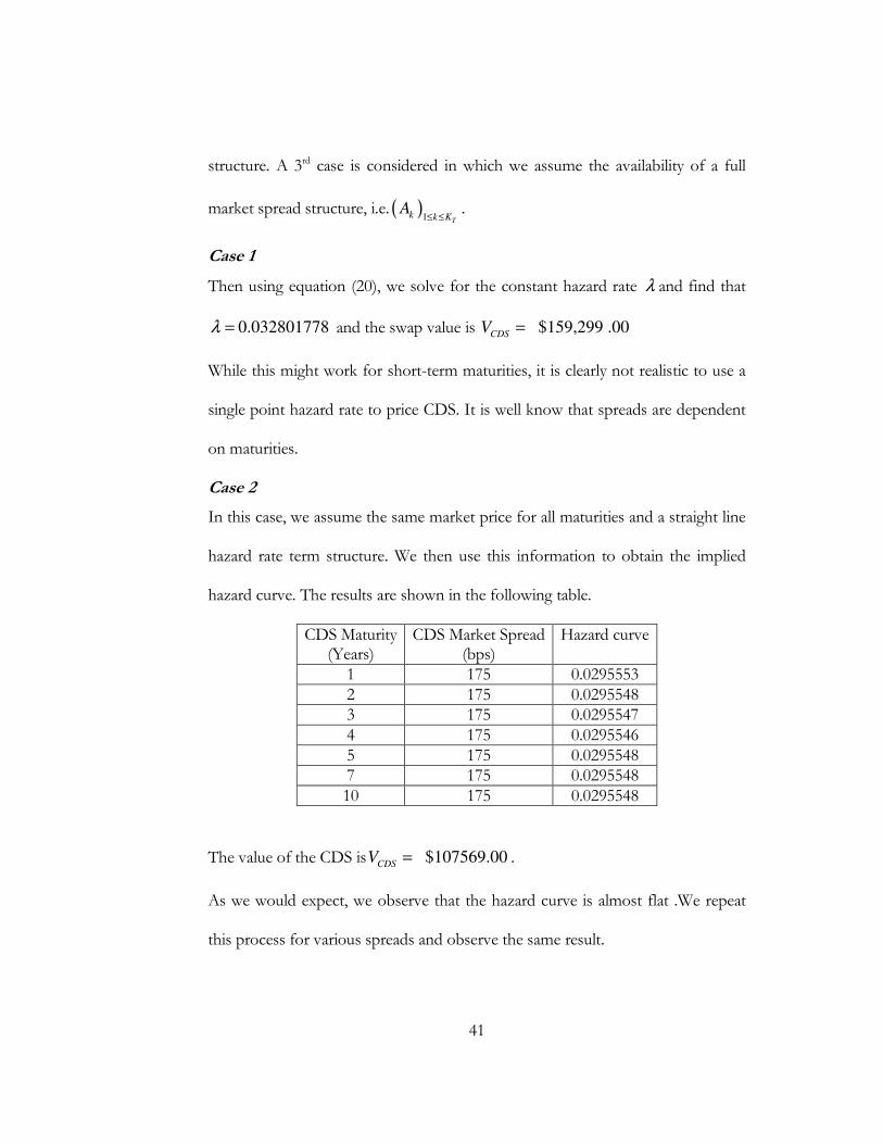
Case 2

In this case, we assume the same market price for all maturities and a straight line

hazard rate term structure. We then use this information to obtain the implied

hazard curve. The results are shown in the following table.

CDS Maturity (Years)

CDS Market Spread (bps)

Hazard curve

1 175 0.0295553 2 175 0.0295548 3 175 0.0295547 4 175 0.0295546 5 175 0.0295548 7 175 0.0295548 10 175 0.0295548

The value of the CDS is $107569.00CDS

V = .

As we would expect, we observe that the hazard curve is almost flat .We repeat

this process for various spreads and observe the same result.

42

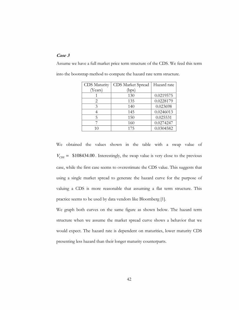
Case 3

Assume we have a full market price term structure of the CDS. We feed this term

into the bootstrap method to compute the hazard rate term structure.

CDS Maturity (Years)

CDS Market Spread (bps)

Hazard rate

1 130 0.0219575 2 135 0.0228179 3 140 0.023698 4 145 0.0246013 5 150 0.025531 7 160 0.0274247 10 175 0.0304582

We obtained the values shown in the table with a swap value of

$108434.00CDS

V = . Interestingly, the swap value is very close to the previous

case, while the first case seems to overestimate the CDS value. This suggests that

using a single market spread to generate the hazard curve for the purpose of

valuing a CDS is more reasonable that assuming a flat term structure. This

practice seems to be used by data vendors like Bloomberg [1].

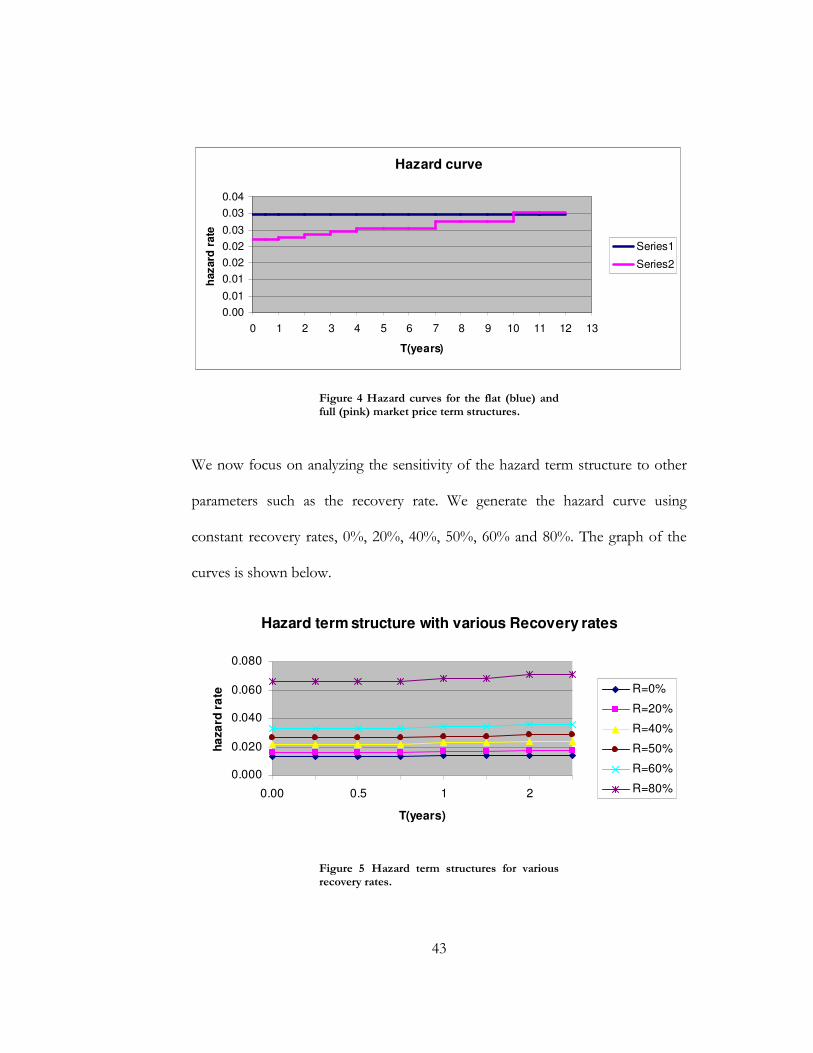
We graph both curves on the same figure as shown below. The hazard term

structure when we assume the market spread curve shows a behavior that we

would expect. The hazard rate is dependent on maturities, lower maturity CDS

presenting less hazard than their longer maturity counterparts.

43

Hazard curve

0.00

0.01

0.01

0.02

0.02

0.03

0.03

0.04

0 1 2 3 4 5 6 7 8 9 10 11 12 13

T(years)

hazard

rate

Series1

Series2

Figure 4 Hazard curves for the flat (blue) and full (pink) market price term structures.

We now focus on analyzing the sensitivity of the hazard term structure to other

parameters such as the recovery rate. We generate the hazard curve using

constant recovery rates, 0%, 20%, 40%, 50%, 60% and 80%. The graph of the

curves is shown below.

Hazard term structure with various Recovery rates

0.000

0.020

0.040

0.060

0.080

0.00 0.5 1 2

T(years)

ha

za

rd r

ate R=0%

R=20%

R=40%

R=50%

R=60%

R=80%

Figure 5 Hazard term structures for various recovery rates.

44

While we observe a similar increasing trend in all curves, we notice that for lower

recovery rates, the spread between curves is minimal and that spread widens as

we go to higher recovery rates. This result is in agreement with what we would

expect. We notice that curves are ordered by the recovery rates. Indeed hazard

rates are higher for higher recovery rates than lower ones as illustrated in fig. 5.

This result is somewhat counterintuitive and evidences the need for further work,

with different models for the recovery rate. For example, one could model the

recovery rate as a stochastic process.

45

Conclusion

The credit derivatives market has known an incredible growth in the last five

years. Since its infancy, along with corporate credit default swaps more complex

products have been developed. One of these complex products is Asset-backed

credit default swaps. In this work, we tried to value the latter using one of the two

approaches used to model credit risk that is a key element in pricing credit

derivatives. The question we tried to answer is whether this approach, the hazard

rate or reduced form approach is applicable to price ABCDS. We have seen that

default payments in ABCDS contract are contingent to the type of credit event,

making it difficult to apply the hazard rate method as in the case of corporate

CDS. To go around this problem, we considered one type of credit event only.

We then implemented a numerical example and obtained a hazard curve that is

consistent with what we expected. Thus the method seems applicable if we

simplify the set of credits events. Further research will require considering each of

the types of credit event as a single jump process and model eventually their joint

distribution as well. We also tested the sensitivity of the method to the recovery

rate and obtained very interesting because of counterintuitive results. This

suggests that further research is needed in this area.

It is evident that pricing ABCDS still presents a challenge. Besides the various

types of credit event in question, another issue is that by the nature of structured

products, there is no direct and linear relationship between default at the tranche

stratum and the collaterals level. This makes it difficult to properly model the

total credit risk, which involves the credit risk at the tranche level but also at the

collaterals echelon. Presently there is no easy way to do take both risks into

account.

46

References

[1] Banc of America Securities, 2004, Credit Default Swap Primer: Market,

Analytics and Applications

[2] P. Billingsley, 1979, Probability and Measure, John Wiley and Sons, New

York, Toronto, London

[3] F. Black, and M. Scholes, 1973, The pricing of options and corporate

liabilities, Journal of Political Economy, 81, 637–654.

[4] ISDA, 2005, Credit Derivative Transaction on Asset-Backed Security (Cash or

Physical Settlement), www.isda.org

[5] Duffie D., Singleton K.: Modeling term structures of defaultable bonds. Rev.

Financial Stud. 12, 687–720 (1999)

[6] A. Elizalde, 2003, Credit Risk Models I, www.defaultrisk.com

[7] A. Elizalde, 2003, Credit Risk Models II, www.defaultirsk.com

[8] C. C. Finger, 2002, CreditGradesTM, Technical Document, RiskMetrics

Group, Inc.

[9] Hughston, L. P., and Turnbull, S., 2001, “Credit Risk: Constructing the Basic

Building Blocks”, Economic Notes, Vol. 30, No. 2, pp. 281-292.

[10] J.C. Hull, 2003, Options, Futures and Other Derivatives (5th edition,

Prentice-Hall)

47

[11] J.C. Hull, and A. White, 2003, The Valuation of Credit Default Swap

Options,

Journal of Derivatives, 10(3), 40–50.

[12] Hull, J. C. and A. White, “Valuing credit default swaps I: No counterparty

default risk,” Journal of Derivatives, vol. 8, no. 1 (Fall 2000), pp 29-40.

[13]J. Hull, I. Nelken, and A. White. Merton's model, credit risk, and volatility

skews. Working Paper, University of Toronto, 2004

[14] Jarrow R and S Turnbull(1995) Pricing derivatives on Financial Securities

subject to credit risk, Journal of Finance, 50 (1), 53-86.

[15] Lando, D.: On Cox processes and credit-risky securities. Rev. Derivatives

Res. 2, 99–120 (1998)

[16] D. Madan and H. Unal, A Two-Factor Hazard-Rate Model for Pricing Risky

Debt and the Term Structure of Credit Spreads, 1999

[17] R.C. Merton. On the pricing of corporate debt: The risk structure of interest

rates. Journal of Finance, 29:449-470, (1974)

[18] R.C. Merton. Option pricing when underlying stock returns are

discontinuous. Journal of Financial Economics, 3:125-144, (1976)

[19] Nomura Fixed Income Research, Credit Default Swap (CDS) Primer, May

12, 2004

[20]-, The Valuation of Multi-name Credit Derivatives, Msc. Thesis, Exeter

College, University of Oxford

48

[21] R. K., Sundaram, 2001, “The Merton/KMV Approach to Pricing Credit

Risk,” NYU Working Paper.

[22] Bank of International Settlements, 2005, www.bis.org

[23] British Bankers’ Association, 2002, www.bba.org.uk