The Utility of Multiple Structure Torsion Angle Alignment

University of South Carolina University of South Carolina

Scholar Commons Scholar Commons

Theses and Dissertations

Fall 2020

The Utility of Multiple Structure Torsion Angle Alignment in The Utility of Multiple Structure Torsion Angle Alignment in

Protein Active Site Description (ASD) Protein Active Site Description (ASD)

Devaun L. McFarland

Follow this and additional works at: https://scholarcommons.sc.edu/etd

Part of the Computer Sciences Commons

Recommended Citation Recommended Citation McFarland, D. L.(2020). The Utility of Multiple Structure Torsion Angle Alignment in Protein Active Site Description (ASD). (Doctoral dissertation). Retrieved from https://scholarcommons.sc.edu/etd/6180

This Open Access Dissertation is brought to you by Scholar Commons. It has been accepted for inclusion in Theses and Dissertations by an authorized administrator of Scholar Commons. For more information, please contact [email protected].

https://scholarcommons.sc.edu/

https://scholarcommons.sc.edu/etd

https://scholarcommons.sc.edu/etd?utm_source=scholarcommons.sc.edu%2Fetd%2F6180&utm_medium=PDF&utm_campaign=PDFCoverPages

http://network.bepress.com/hgg/discipline/142?utm_source=scholarcommons.sc.edu%2Fetd%2F6180&utm_medium=PDF&utm_campaign=PDFCoverPages

https://scholarcommons.sc.edu/etd/6180?utm_source=scholarcommons.sc.edu%2Fetd%2F6180&utm_medium=PDF&utm_campaign=PDFCoverPages

mailto:[email protected]

THE UTILITY OF MULTIPLE STRUCTURE TORSION ANGLE ALIGNMENT IN

PROTEIN ACTIVE SITE DESCRIPTION (ASD)

by

Devaun L. McFarland

Bachelor of Science

St. Lawrence University, 2009

Master of Engineering

University of South Carolina, 2012

Submitted in Partial Fulfillment of the Requirements

For the Degree of Doctor of Philosophy in

Computer Science

College of Engineering and Computing

University of South Carolina

2020

Accepted by:

Homayoun Valafar, Major Professor

Jijun Tang, Major Professor

Marco Valtorta, Committee Member

Michael Huhns, Committee Member

Kim Creek, Committee Member

Cheryl L. Addy, Vice Provost and Dean of the Graduate School

ii

© Copyright by Devaun L. McFarland, 2020

All Rights Reserved

iii

ABSTRACT

Proteins are responsible for various functions throughout organisms, or within the

systems, they operate. Active-sites or functional/ binding sites are regions responsible for

activity in a protein; they serve as a catalyst for reactions, attach or bind to other

molecules (ligands), and maintain function. With the profusion of protein sequence and

structure data, it's increasingly relevant to develop automated methods of identifying and

investigating active-sites for proteins. Active-sites identification will have a direct

impact: in better understanding molecular basis for diseases, assisting in drug design, the

study of targeting mutants, and for functional annotation of unknown proteins. The

proper knowledge of active-sites will also be beneficial in protein design and

engineering. Existing computational approaches to active-site identification fall short of

the ideal. Several approaches fail to include some critical information, such as, global

structure, local structure, amino acid position, and local biochemical properties. Here we

present msTALI (Multiple Structure Torsion Angle Alignment) to better understand and

characterize protein sequence-structure-function relationships.

The existing studies establishing our understanding of active-sites stress the importance

of sequence, structure, and biochemical properties of proteins in their function.

Therefore, an ideal method for active-site analysis should consider all the information

above. The msTALI tool is unique compared to other existing software in that it

incorporates sequence, structure and biochemical properties of amino acids to perform its

analysis. Furthermore, msTALI generates competitive results and exhibits an ability to

iv

address proteins undergoing rigid-body motion. Additionally, the customization

capability of msTALI makes it an expandable algorithm; suitable for the valid

identification of active-sites.

We utilize msTALI successful structural alignment capabilities under premises

for active-site studies. The theoretical background is paramount since the research is

interdisciplinary. We discuss molecular biological constructs, relate such descriptions to

active-site research, survey previous methods, and expand our methodology. The

msTALI software is used first to examine sets of proteins with confirmed ATPase

activity. We use several fold families to evaluate effectiveness. Additionally, we map the

trajectory for additional studies with upward of ten functional classes of proteins to

strengthen the targeting set of proteins for observation. Collectively, findings will expand

the understanding of active-sites, yield development for automated site description, and

generate the programmatic development of software.

v

TABLE OF CONTENTS

ABSTRACT .......................................................................................................................... iii

LIST OF TABLES .................................................................................................................. vi

LIST OF FIGURES ................................................................................................................ vii

LIST OF ABBREVIATIONS ..................................................................................................... ix

CHAPTER 1: INTRODUCTION: INTRODUCTORY BIOLOGY .......................................................1

1.1 PROTEINS...............................................................................................................2

1.2 ACTIVE SITES ........................................................................................................3

1.3 PROTEIN STRUCTURAL ELEMENTS ........................................................................4

CHAPTER 2: ACTIVE SITE DESCRIPTION (ASD) ...............................................................6

2.1 PREVIOUS WORK ................................................................................................10

2.2 SUMMARY ...........................................................................................................13

CHAPTER 3: THE MSTALI ENGINE ......................................................................................14

3.1 MSTALI ENGINE DESCRIPTION ...........................................................................14

3.2 DETAIL OF WORK: OVERALL VIEW .....................................................................16

CHAPTER 4: UTILIZING MSTALI FOR ASD .........................................................................34

4.1 METHODOLOGICAL DEVELOPMENT FOR ASD USING MSTALI ............................34

4.2 APPLICATION TO STUDIES THROUGH MSTALI .....................................................53

CHAPTER 5: DISCUSSION .....................................................................................................97

REFERENCES .....................................................................................................................100

vi

LIST OF TABLES

Table 3.1 Target Proteins of Study ....................................................................................23

Table 4.1 Protein Alignment Count ...................................................................................44

Table 4.2 Comparing Alignment Descriptions ..................................................................46

Table 4.3 Recording Conserved Residues for Steroid Targets. .........................................48

Table 4.4 Comparing the Mode of Alignment for Proteins Studies ..................................53

Table 4.5 ATPase Target Protein Overview ......................................................................56

Table 4.6 Secondary Structure for ATPase Target Proteins ..............................................57

Table 4.7 Program Evaluation Comparison on Fold Families ...........................................65

Table 4.8 The Primary Precision and Recall for Our Approach ........................................69

Table 4.9 Annotation for Focused Study Proteins .............................................................76

Table 4.10 The Prominent Protein Features for the ASD on Focused Studies ..................77

Table 4.11 Gene Expression Inhibiting Residues of Interest .............................................80

Table 4.12 Preliminary Protein List Related to NSP1 Functional Activity .......................80

Table 4.13 Surface Accessibility for Conserved Regions of NSP1 ...................................81

Table 4.14 Reporting Conserved Regions for Protein 6LU7 .............................................90

vii

LIST OF FIGURES

Figure 1.1 An Alpha Helix...................................................................................................7

Figure 1.2 A Beta Sheet .......................................................................................................8

Figure 1.3 Coil Regions .......................................................................................................9

Figure 3.1 Core Markup of msTALI Alignment. ..............................................................27

Figure 3.2 Job Submission Options for msTALI ...............................................................29

Figure 3.3 ASD from msTALI Results ..............................................................................31

Figure 3.4 Phylogeny tree Annotation ...............................................................................33

Figure 4.1 The Numerical Requisite for Proteins Aligned with msTALI .........................42

Figure 4.2 The Requisite Description on Steroid Functional Class ...................................49

Figure 4.3 The Active-Site for 1ATP-E .............................................................................58

Figure 4.4 The Super Imposition of Protein Fold Families ...............................................63

Figure 4.5 Confirmed Protein Information for Precision and Recall ................................64

Figure 4.6 The Conserved Core Regions ...........................................................................66

Figure 4.7 Active-Site Identification ROC curve ..............................................................71

Figure 4.8 Highlighting the ASD for Protein 1FLM .........................................................74

Figure 4.9 The msTALI Conservation Score for SARS-CoV-1 NSP1 .............................83

Figure 4.10 The Visual Rendering of Wild-type NSP1 .....................................................84

Figure 4.11 The msTALI Conservation Score for Templated Set .....................................87

Figure 4.12 The msTALI conservation score for protein 6LU7 ........................................89

Figure 4.13 The Picture Representation of Protein 6LU7 .................................................94

viii

Figure 4.12 Templating the ASD for Protein 6LU7 with 7BTF I .....................................95

Figure 4.13 Templating the ASD for Protein 6LU7 with 7BTF II ....................................96

ix

LIST OF ABBREVIATIONS

AMP ........................................................................................... Adenosine monophosphate

ASD.................................................................................................. Active Site Description

ATP .................................................................................................. Adenosine triphosphate

BsFinder ................................................................................................. Binding Site Finder

CO ................................................................................................. Continuous Optimization

FAD........................................................................................... Flavin adenine dinucleotide

FFF ................................................................................................. Fuzzy Functional Forms

FMN ..................................................................................................Flavin mononucleotide

GLC.......................................................................................................................... Glucose

MolLoc ...................................................................... Molecular Local Surface Comparison

msTALI .......................................................... Multiple Structure Torsion Angle Alignment

NAD ...............................................................................Nicotinamide adenine dinucleotide

NN .............................................................................................................. Neural Networks

pdbFun ...................................................................................... Protein Data Bank Function

PDBsum ................................................................................... Protein Data Bank summary

PO4 ....................................................................................................................... Phosphate

ROC ....................................................................Receiver Operating Characteristic (curve)

SiteEngine ................................................................................ Site Engine (for active sites)

SuMo ......................................................................................................... The SuMo Server

VMD ........................................................................................ Visual Molecular Dynamics

Web-app ................................................................................................Website Application

1

CHAPTER 1

INTRODUCTION: INTRODUCTORY BIOLOGY

Herein, research is interdisciplinary work that includes topics from Biological and

Computational Sciences. We focus on proteins with the aim to understand function. The

objective is to establish a body of work efficiently comparable to current functional

studies, given the breadth of biological data available. Additionally, we discuss how our

methodology will suitably address protein function and contribute to the field.

Within a bubble or rather, under a controlled environment, the intricacies of

protein interaction can be captured and observed. Still, there is more to research. Though

simple to grasp, the concept of these biomolecular constructs working as portions of a

whole is also demonstrative of complex relationships and numerous interactions; this

truly sets the tone for a plethora of valuable protein studies. Notably, as topics in

bioinformatics/ computational biology would suggest; we use computers to aid in

genomic studies whether they are a sequence, structure, and or functionally based

construct. Addressing what transpires/ the true "how to" concerning proteins themselves

and with specialization, at that, is difficult. What is it that distinguishes the required input

forming organs such as the heart or intestine? How do we characterize the function of

proteins based on all contributing factors using a consistent methodology? Exploration of

protein function is salient, and the interactions of bindings amongst each protein serve as

a point for foundational reference. Active-sites identification will have a direct impact: in

better understanding molecular basis for diseases, assisting in drug design, the study of

2

targeting mutants, and for functional annotation of unknown proteins. The proper

knowledge of active-sites will also be beneficial in protein design and engineering.

Definitively, active-sites are regions where bindings occur and describe protein function.

We discuss approaches for active-sites identification. We first describe protein makeup

for component features and functionality. Then we explicitly specify the functionality and

expansions on active-sites identification for our research. The contribution and

methodology is novel and will utilize the preexisting in-house software. Development of

a revamped interface coupled with a submitted application to active-sites identification is

the target. We outline studies used for testing our existing software to build the

framework for development.

1.1 PROTEINS

Proteins constitute an important class of biomolecules that are analogous to

workers in a factory. Proteins account for both the makeup and execution of functions

carried out by cells. Describing the hierarchy, bundles of cells uniquely form tissue, and

tissues formulate organs. At the highest level, we understand that organs are the self-

contained components for living beings and further each serves vital roles in life

processes; one's heart or brain does not perform the tasks of the liver or intestine. It is

increasingly evident that proteins are an agent of how our bodies work. Ergo, it is equally

vital/ there is much value in understanding what proteins are.

As termed, proteins are called polypeptides because peptide bonds conjoin several

amino acids. Describing proteins in this manner yields information relating to proteins

sequence. The sequence outlines the amino acid chains that formulate the protein.

Generally, several amino acids make up a single protein and attribute to a proteins length.

3

Lengths can vary, and account for diversity amongst any set of proteins. For example,

here, we study proteins ranging from hundreds to thousands in length, with average sizes

being roughly 300 amino acid residues. Generally, these lengths are described as

residues because we are referring to molecules bonded to each amino acid in the protein

sequence [1].

Interestingly enough, though proteins vary in length the combinations of

sequences are comprised of 20 primary amino acids. Each amino acid has an acronym

used for labeling the sequence description which can be described as follows: Alanine

(A), Cysteine (C), Aspartic acid (D), Glutamic acid (E), Phenylalanine (F), Glycine (G),

Histidine (H), Isoleucine (I), Lysine (K), Leucine (L), Methionine (M), Asparagine (N),

Proline (P), Glutamine (Q), Arginine (R), Serine (S), Threonine (T), Valine (V),

Tryptophan (W), and Tyrosine (Y) [1].

Nonetheless, the arrangement of these 20 amino acids varies and when discussed

concerning their chemical properties, account for more detailed descriptions of the

proteins we study. In fact, not only do these 20 amino acids and protein properties

account for diversity amongst proteins themselves; each also performs functions based on

the organism or system they are inherently used. The function relates to bindings, and, as

such, we elaborate on active-sites; they are the area of focus for these studies.

1.2 ACTIVE SITES

Active-sites are areas where reactions and binding events take place and therefore,

they describe a protein's function. They are synonymous with binding sites and or

binding regions, as they apply to enzymatic and cofactor relationships that are indeed,

actually reacting in some way. Hitting home, these locations on proteins are active and

4

responsible for conjoining relationships like that of a puzzle; pieced or bound together.

Further, the functional regions catalyze change within the system. Active-sites typically

are described as regions on proteins demonstrative of some prominent features. For

example, active-sites exist in clefts or pocket regions of proteins. Considering the

globular nature of a protein surface, this makes sense. Mentioning the surface of proteins

is essential too. Active-sites though sometimes found in the back of cleft regions, also

have attributes or valuable structural components which make them surface accessible or

partially exposed during the dynamics undergone with protein function; these changes

can be chemical too. Identifying active-sites relies on biologically confirmed information,

especially to date. We recognize conserved regions as the areas of a protein that is

structurally similar or important to structural alignments obtained from our approach.

Conserved regions are then used for active-site identification by referring to biologically

confirmed annotations. The coupling of the two promotes the foundation of information

causal to application development; our methodology first developed for structural

alignment is implement with a new interface and applications specific to active-sites.

Next we describe the purely structural elements of proteins.

1.3 PROTEIN STRUCTURAL ELEMENTS

Proteins are characterized chiefly by having primary, secondary, and tertiary

structure. Primary structure refers to a proteins sequence-based information. The

characteristics depicted by its amino acid chain, as mentioned in the previous section.

Secondary structure and tertiary structure refers to the shape of a protein, each of which

we can elaborate on further. Not of focus is quaternary structure as it pertains to proteins

shape in complex or folded units.

5

1.3.1 Secondary Structure

With the orientation of amino acid chains comes the fold developed by bonds of

the molecules within each residue. The interactions between residues are critical to shape.

Secondary structures are descriptions of the central backbone atoms. They include Alpha

Helices (α-helices), Beta Sheets (β-sheets), and coil regions. Notably, it is the hydrogen

bonding that causes these centralized shapes. An α-helix is a structural motif categorized

by a spiraling shape as pictured in Figure 1.1. Similarly, Figure 1.2 displays a β-sheet

which is formed by two β-strands (yellow) which fold somewhat parallel to one another

like two flat layers or planks. Coil regions are essentially areas within proteins where the

structures don't fit a particular motif but may be dynamic or flexible in conformity

(Figure 1.3). Secondary structures in this regard, describe shapes within a protein, but

may not explain the global structure for a protein.

1.3.2 Tertiary Structure

Tertiary structure describes the overall three-dimensional (3D) shape of a protein.

They illustrate both the central backbone and side chain components of each amino acid

bonded within that particular protein. The folds and the shape of a protein form due to

chemical interactions. Bonding properties as mentioned before, attractive and repulsive

forces, and even hydrophobic interactions play a role. Further, regardless if it is the

molecular collisions allowable or its relationship with water, acceptable folding and

shapes of proteins are relevant for description, classification, and functionality. We

explore all of these structural elements and more when employing our approach and

further investigating our active-site studies.

6

CHAPTER 2

ACTIVE SITE DESCRIPTION

In this work, we define active-sites as locations on proteins that are causal to

function. An active-sites size, location, and chemical components all affect the function

and need of proteins within the system they operate. Moreover, if proteins demonstrate a

similar role, then those same proteins will also have mirroring structural similarities. Our

direct premise and novel approach for active-sites description (ASD) supports this notion.

Our definition for ADS is to provide the location and central regions on a protein needed/

necessary for protein function. The problem is developing a methodology that does this

reliably. Capturing the direct relationship between the function and structure of a protein

is critical in better understanding the mechanism of its function. The sequence-structure-

function relationships for proteins need be unbroken. This task embodies intricacy since

such relationships require accurate descriptions that are not always classified or

recognizable. It turns out that several factors contribute to functionality; conformity,

location, size of active-sites, ligand binding properties, and regions of proteins that are

surface accessible, all play a role.

Further, it isn't known which of these factors affect function most. The inherent

problem is the development of an automated methodology, inclusive of all factors, that

successfully identifies binding regions and the most significant structures. To this matter,

a completing ASD through computational methods is addressed.

7

Figure 1.1 An Alpha Helix. Here we see a secondary structure characteristic common to protein structure.

8

Figure 1.2 A Beta Sheet. Here we see a secondary structure characteristic common to protein

structure. Note: Beta sheets are beta stands folded with relationship to each other, each yellow

portion constitutes a strand.

9

Figure 1.3 Coil Regions of proteins. Here we see a secondary structure

characteristic of proteins that are more flexible. A. illustrates a bend or

turn region (cyan) and non-secondary structure features (coil/ grey) that

are non-continuous. B. are continuous coil regions, here we also see beta

bridge structures in gold. C. A 3/10 helix structure.

10

2.1 PREVIOUS WORK

Computational methods of identifying active-sites on proteins have been

introduced as early as 1960. Since then more advanced computational methods

incorporating graph-theoretic or even probabilistic techniques have been presented with a

substantial contribution to the field. While these methods have demonstrated progress,

they exhibit individual shortcomings that need to be addressed. In the following sections,

three classes of the most advanced techniques are reviewed concerning approaches that

employ common strategy types, and we outline their strengths and weaknesses.

2.1.1 Method One: Geometric and Graph-based Approaches

One intricacy with ADS manifests in the shapes of proteins themselves. Surface

representations for proteins demonstrate their globular nature. There is an unevenness

witnessed on the protein surface [2], which makes it relevant to utilize docking

techniques to explore interactions. A simple description of docking strategies

characterizes enzymatic activity or how proteins engage with any of their cofactors at the

surface level, i.e., binding regions for active-sites by attempting to piece them together

like a puzzle. Our first methods use geometric principals and graph-based ideologies for

the problem. Geometric approaches are starting points mapping the proteins space, from

which, grids are used [3]. Here we mention POCKET, which is a reliable tool and

algorithm since its geometric nature is straightforward. The surface of a protein is

scanned based on Cartesian coordinates. The grid points are used to describe distances

and available reliefs and anomalies on the protein surface, to define them as clefts/

pockets. The method scans for pocket areas subject to docking without prior knowledge

11

of binding site location [3]. However, the orientation of the protein needs to be constant

in the grid space.

Additional grid-based methods like LIGSITE aim to reduce Cartesian dependency

by adding other orientation perspectives [2]. Increasing orientation perspectives is precise

for pocket detection but requires more calculation. Geometric tools serve beneficial since

they are accurate and map the protein space. Though it is difficult to pinpoint the end of

pockets and free space markers, these graphing techniques dominate the field; they

require no prior knowledge and measure clefts/ pockets observable on proteins. They fall

short of ideal due to a dependency on grid orientations, and circumventing these restraints

requires more calculations typically.

2.1.2 Method Two: Ranking and Learning Techniques

It is evident that the cavity features are relevant [4]. Improvements for geometric

or graph-based tools are developed by focusing on cavities or the pockets themselves.

CAST is a computational method that identifies and measures the size of pockets using

graph-based attributes and modeling techniques. Convex hull representations provide

shape descriptions and are beneficial for both scientific significance and binding

reliability [4]. The size of a pocket will allude to what can and cannot bind to a specific

region. From this contribution, it is common to incorporate cavity/ cleft region rankings,

categories, and representations [5][6]. Specifically, research suggests that when several

clefts are detected ranking them by size is essential. Using bounds around the structures

further demonstrates that more often than not, the larger cavity is responsible for binding

[7]. Here we see an even stronger representation of a proteins surface structure

12

representation. However, surfaces and some principal components for function are not

static. Surface variation is common, and these approaches do not account for dynamics.

Ranking and predicting clefts for active-sites expands to other catalytic locations

on proteins that are dynamic and facilitate functions. Graph-theoretic methods also

incorporate hashing techniques for feature recognition [8]. Since these relationships aren't

direct fuzzy functional forms (FFFs) are adapted to practice [9][10]. FFFs aid in exposing

the notion that fold families must be able to perform several functions. A FFF approach

does well for annotating proteins and finding motifs for ASD. The disadvantage comes

when trying to match motifs to novel structures [11]. Procedures then apply Neural

Networks (NN) for comparing the structure-function similarities [11]. NN training tactics

learn the likelihood protein residues are indeed catalytic. NN is reliable for working with

novel structures but are subject to improper training for proteins with multiple or unique

catalytic regions of any particular sub-family [11]. Collectively, ranking cavities and

applying learning techniques for ADS is advantageous for further classifying essential

protein structures, notating motifs, and learning emerging proteins. The disadvantages of

these methods standout when considering dynamics; they fail when working with flexible

binding sites too.

2.1.3 Method Three: Online Tools

Several web services are aiming to address ASD also [12][13][14]. We utilize

them as comparison methods to discuss our approach which works since they are all

based on the similar established frameworks/ background information. We see that

Continuous Optimization (CO) creates a pairwise comparison between two proteins to

address functional regions [8]. Further, Molecular Local Surface Comparison (MolLoc)

13

does too [15]. SiteEngine is a recognized method for pairwise docking descriptions with

hash triangles [16]. SuMo incorporates chemical groups with structural representations

[13], and pdbFun is a web service that breaks its analysis at the residue level [17].

Binding Site Finder (BsFinder) methodology provides a three-step process similar to our

goal since it incorporates sequence and structure info [18]. These methods supply a visual

platform. The overarching shortcoming is each of these examples fall victim to the

limitations mentioned above. Additionally, the approaches trend to identify active-sitess

with precisions not exceeding a 65% success rate. A valuable rate considering the nature

of the problem, but there is room for improvement.

2.2 SUMMARY

There are shortcomings concerning some critical information for the more

extensive description of active-sites. It is considered worth noting that within the

drawbacks, most approaches focus on the annotation of an individual protein or utilizes

two proteins to establish binding qualities. We find it beneficial to regard groups of

proteins. Our Multiple Structure Torsion Angle Alignment (msTALI) approach addresses

many of the deficiencies concurrently while observing multiple proteins simultaneously

[19]. We generate competitive results and utilize our platform to study sets of proteins in

entirety since they too are dynamic. We consider the global and local structure, amino

acid position, and local biochemical properties. Our methodology takes advantage of the

existing engine by performing superior alignments on proteins that are documented to

achieve the same function, all while detecting dynamic confirmations; this becomes key

when addressing proteins classified with a similar role, that bind flexible ligands, and that

are non-homologous [20].

14

CHAPTER 3

THE MSTALI ENGINE

The msTALI is a hybrid 1D - 3D method designed to perform structural

alignments on multiple proteins simultaneously [19]. In this project, we leverage the

existing msTALI software to develop an active-sites identification mechanism. This

chapter details explicitly the msTALI Engine, for existing functionality. The msTALI is

currently an in-house, stand-alone web-application with downloadable executables

flexible enough for expansion. So in this regard, we will mention the current core engine/

algorithm. Our Research describes programmatic development/ expansion by way of a

new interface that incorporates the existing functionality expanded and applied to

problems focusing on ASD. We describe msTALI in detail, and, we outline the work in

utilizing msTALI for ASD in proteins.

3.1 MSTALI ENGINE DESCRIPTION

The msTALI software package, developed by the ValafarLab is available for

download and use from the following URL: http://ifestos.cse.sc.edu [19]. The msTALI

approach exhibits distinct advantages over other comparable approaches as highlighted in

previous publications [19]. The TALI/ msTALI software package take advantage of both

sequence and structural information to achieve better performance. Previous work

demonstrates the success of TALI [21] and msTALI [19] as an approach which uniquely

adheres to conditions that make our task difficult. The msTALI engine is an extension of

TALI by including multiple structure alignment in a manner that is analogous to

http://ifestos.cse.sc.edu/

15

ClustalW [22]. Our approach to structure alignment sets itself apart from other

methods by including structural information such as backbone torsion angles, atomic

positions, and membership of each residue in a secondary structural element, while

including alignment of sequences using the Needleman-Wunsch [23] algorithm. The

msTALI engine also includes other information such as water accessibility, structural

information of side-chains (which are essential in the biochemistry of the enzyme), and

properties of the neighboring atoms. The msTALI core engine applies these features

using a scoring metric to calculate structural alignments. We highlight the metric with

equation one, Eq. (1), it defines the function of the global dynamic programming

algorithm [19].

S(𝑟𝑖 , 𝑟𝑗) = 𝑤𝑡𝑡(𝑟𝑖, 𝑟𝑗) + 𝑤𝑏𝑏(𝑟𝑖, 𝑟𝑗) + 𝑤𝑟𝑟(𝑟𝑖, 𝑟𝑗) + 𝑤𝑠𝑠(𝑟𝑖, 𝑟𝑗) (1)

+𝑤𝑑𝑝𝑑𝑝(𝑟𝑖, 𝑟𝑗) + 𝑤𝑠𝑝𝑠𝑝(𝑟𝑖, 𝑟𝑗) + 𝑤𝑑𝑠𝑑𝑠(𝑟𝑖, 𝑟𝑗) + 𝑤𝑠𝑠𝑠𝑠(𝑟𝑖, 𝑟𝑗)

Here, weights denoted by w subscripts, are normalized to one and applied to each scoring

feature. Features being: torsion angles (t), the backbone 𝐶𝛼 atom position (b), residue

type (r), secondary structure type (s), and properties of nearby atoms based on distance to

and sequence types (𝑑𝑝, 𝑑𝑠, 𝑠𝑝, 𝑠𝑠). Each evaluates and compares the score matchings for

any corresponding residues i and j. Note, however, that the score "S(𝑟𝑖, 𝑟𝑗)” is used by the

engine to obtain an optimal score based off of structural alignment from one residue to

the next residue.

By incorporating this framework to design, and by using a flexible platform, the

application is expandable to apply to our active-sites studies. Our work falls into two

parts, methods development, and usability and web development (maybe software). Our

next sections elaborate on the framework that will be used for the study. We aim to

16

master approaches conducive to ADS while anticipating difficulties that might occur. We

outline how to address pitfalls make our approach more reliable.

3.2 DETAIL OF WORK: OVERALL VIEW

The outlined research consists of the following three specific aims:

1. Development of a methodology for ASD using msTALI – The primary objective

of this research is the adaptation of msTALI for use in ASD. In doing so, our lab

resources will be updated and current, improvements to the computational methodologies

for active-sites identification explored, and we will contribute to research of the common

core while expanding knowledge and mastering understanding for current practice. The

background for the study is extensive, in that, in-depth exploration of computational

approaches is necessary. Further, surveying such attitudes becomes interdisciplinary and

establishes the framework for experimental procedures.

2. Optimizing the parameters of msTALI for ASD – We anticipate that as the

functions of proteins change, so will the intricate attributes that contribute to the changes.

For example, some proteins might have physical components that are responsible for

facilitating function; a door, gate, or hinged region that enables binding. In these cases, it

would make sense to increase the significance of parameters that weigh secondary

structural importance. With msTALI, we can adjust features independently. The msTALI

engine uses scoring features that quantify the effectiveness of structural alignments. If

needed, we are prepared to conduct studies optimizing msTALI’s operational parameters

specific in use for ASD because it could prove critical to our methodology.

3. Development of a user interface useful for ASD studies – Working to develop a

new interface for msTALI is relatively simple to describe since this stage is ongoing.

17

Several of the features are beneficial to usability for conducting studies. We discuss

changes to the web-presence to provide aesthetics advantageous to methodology.

However, catering msTALI to ADS is a robust process that will require more than

website changes since the upgrades mirror our three thrusts directly to practice.

Contributions will primarily fall into three categories in conjunction with research

studies. Classes being: the methodology for discovering active-sites with msTALI,

optimizing the preprogrammed parameters within the msTALI engine for ADS, and

usability for the user interface improvements.

3.2.1 Aim 1: Development of a Methodology for ASD Using msTALI

We will develop and evaluate a process that is advantageous in the identification

of active-sites. Our developments proceed based on the underlying hypothesis that

structure-sequence alignment of multiple proteins with common function will reveal the

conserved regions (structural and sequence), which must contain the active-sites and

motifs salient to functionality. The initial strategy that we will pursue will depend on the

alignment of multiple structures with a similar function using msTALI. However, we

anticipate the following scenarios when aligning proteins. There will be active-sites not

recognized by our conserved region alignments. These more detrimental conditions are

attributed to various factors which make ASD challenging to define.

With our first scenario, we state that some active-sites will be underrepresented

because several proteins perform more than one function. This scenario confuses our

approach based on function prominence, or perhaps by failing to separate the functions

appropriately. Provided the possibility that proteins perform more than one function, we

propose documenting all of the reported ligands and cofactors each protein binds. We

18

will use the PDB [24] to collect binding information. Our initial test will align the

proteins based on a single common functionality. Then we will incorporate the

documented subcategories of functions for subsequent use based on any additional

functionality. Through reporting and subsequent use (based on multiple protein

functions), we will use the subsets of regions returned from msTALI as a collection of

information pertinent to ASD.

We also anticipate the case that conserved regions will stand out, but will

demonstrate residue shifts left or right of the documented sequence location. We attribute

residue shifting to the numbers of residues within a sequence alone being limiting for

ASD. For example, let’s say, the documented active-sites is recorded at residues five

through seven for some given protein. Then our results return residues numbered eight

through ten. Our location at this point is described primarily by numerical information

based on sequence position. Sequence formation alone is not enough. Structurally,

residues on either side of our hypothetical example, and even further away in residue may

be central to functionality when considering the spatial location on the protein. To

overcome this pitfall, we will again, train using the proteins with the same function. Then

we visualize the three-dimensional shape of each protein. Visualizing protein shape will

test and assure that left or right shifts of any documented active-sites residues are in a

respectable local considered important to ASD. We will report the shifts as an acceptable

threshold for accurate alignments for ASD directly.

The third scenario that we anticipate contributing to pitfalls in our approach

combines the notion that the actual functional regions of proteins are flexible for some

ligands, and proteins themselves have different structural domains/ classifications. In

19

other words, for one protein a functional region might reveal itself easiest if the protein is

in some conformation “A” instead of “B.” We will test this in the method by using

phylogenetic information, in conjunction with protein shape descriptors to additionally

group and realign proteins as we did in the first scenario. Our shape description will come

from researching CATH [25] information for each target protein. We then proceed with

our approach by naively passing the structures for alignment based on the functional

similarity. However, we are now prepared to address instances where the simple

alignment yield inconsistent conserved core regions for ASD. We account for protein

dissimilarity where specific protein motifs may be less prominent in some conformations

and more in others. We can now assume that conserved core regions will stratify into

groups; some uniform and others, not so much. This divergence is challenging and

additionally attributed to proteins performing multiple functions, as mentioned in our first

scenario.

Consequently, our approach is intricate in practice when using our annotation. In

proposing, the incorporation of all annotations has to be performed in a manner that

monitors the apparent difference in groups, but not too much to where sensitivity is

neglected. We want to capture the most valuable information about what is conserved for

function by including each aspect of our approach. From here, we focus on what regions

are conserved from clusters of focused information.

Our ADS features will include conserved residues consistent across a total dataset

of proteins, and essential residues characteristic to binding sites. Collectively the above

displays motifs for functional classes. Additional attributes yielding from our approach

include annotation and secondary structural information, with an ability to align novel

20

proteins that one might envision mapping to a particular function. Again, we proceed

based on the hypothesis that structure-sequence alignment of multiple proteins with

common function will reveal the conserved regions (structural and sequence), which must

contain the active-sites. Our methodology is advantageous when compared to existing

computational methods since we observe several proteins at once.

Overall when establishing our approach for ASD, we first need to input our

proteins structures to the msTALI software. We utilize groups of proteins (ten to twenty

at a time) and use the collection for analysis (which can also be referred to as training) by

msTALI. In practice, we also record the length of proteins. Protein length affects how

many times a set of proteins undergoes training. The number of trained observations is

always less than an adjustable percentage of a proteins length (measured in residues). We

do this to avoid overfitting; it also limits the number of returned conserved regions for

proteins with high structural similarity. The msTALI alignment is conducted on the

complete group of proteins simultaneously. Here, we record the conserved residues

obtained by the analysis and evaluate phylogenetic results with CATH classification. This

classification is pivotal for our next round of training. We continue to train on each subset

grouping of the proteins, in this instance, grouped with similar phylogeny and CATH

classification. We record the number of conserved core residues again. We compare the

number of conserved regions obtained from simultaneous alignment to the number of

conserved regions obtained by our sub-classification training. Typically the simultaneous

groupings will have less conserved core residues. We use the number of conserved

regions from the simultaneous alignments with the number of conserved regions from the

sub-classification training as bounds; they are lower and upper limits respectively. The

21

range of conserved regions is valuable for ASD. We use the range and an acceptable

threshold related to protein length for conserved regions we consider reliable for the

ASD.

Our methodology for ASD uses data obtained by the structural alignment of

several proteins displaying the same enzymatic activity. Each class of protein will be

submitted to msTALI as input separately. We use a collection of ten protein classes to

validate our method. Our protein classes include AMP, ATP, FAD, FMN, Glucose,

Heme, Hydrolase, NAD, Phosphate, and Steroid functioning proteins. Each subgroup will

start with a simultaneous run of the proteins to msTALI, categories comprised of roughly

15 proteins each. Table 3.1 lists our target proteins. Thus, we assess multiple proteins

while covering a diverse spread of classified protein groups commonly studied by the

field.

Verifying the success of the method for ASD relies on biologically confirmed

information. Upon concluding the complete approach on each set of proteins, we then

observe results for biologically confirmed annotations. VMD [26] will be utilized to

visualize the results of our approach. Additionally, the inclusion of additional proteins to

each set validates results. For example, say a protein is confirmed to have AMP binding,

we can add that new mentioned protein to our studied run to evaluate consistency.

Further, this templating type test can be performed on proteins – tentatively even

novel proteins – if they indeed do fit within a particular class of proteins with a function

in mind. With this methodology in mind, we can now discuss additional contributions to

the research outlined by our thrust. We have anticipated that our method might require

parameter changes as detailed in section 3.2.2 collectively; we also mention the interface

22

changes in section 3.2.3 all to provide a well-rounded solution to our researched method

for ASD.

3.2.2 Aim 2: Optimizing the Parameters of msTALI for ASD

The existing implementation of msTALI is optimized for general alignment of

multiple structures. The investigations highlighted in Aim1 will help to establish the

utility of msTALI in the specific domain of active-sites identification. Aim 2 of our work

serves as a contingency plan in the event that optimizations of the parameters described

in Eq. (1) for application in ASD are required. As needed, we will investigate the

optimization of weights for ASD or optimization of weights for each class of enzymatic

activity

From an overall standpoint, it is possible that there will be a single set of weights

that works advantageously for all the studied targets for ASD. For example, and provided

some general use, we can adjust all weights in a manner such that, the normalized values

mirror characteristic reflective of concepts highlighting functional concerns. It is well

known that locations responsible for function within a protein are dynamic. ASD

incorporate regions of proteins within clefts, areas that may be surface accessible, and

have chemical properties; weights would be adjusted to address these complex

combinations. So, through algorithmic design, optimizing the used parameters for

msTALI scoring metric explores weighted features – surface accessibility, for example –

of protein residues, but also alignments based off of flexible or custom components and

not just the core, can improve an ASD.

23

Table 3.1 Target Proteins of Study. We have listed, in tabular form, the proteins we will study by named grouped by their protein

classes (additional proteins for Hydrolase class include: 5F9R, 5K8I, 5KSO, 5LHB, and 5M0X. For Phosphate class include:

1L7Ma, 1LBYa, 1LYVa, 1QF5a, and 1TCOa. are listed here for spacing).

Target Protein classes

AMP ATP FAD FMN Glucose Heme Hydrolase NAD Phosphate Steroid

Pro

tein

Nam

es

1AMUa 1A0Ia 1CQXa 1DNLa 1BDGa 1D0Ca 1GTP 1HEXa 1A6Q 1E3Rb

1C0Aa 1A49a 1E8Gb 1F5Va 1CQ1a 1D7Ca 1RYA 1IB0a 1B8Oc 1FDSa

1CT9a 1AYLa 1EVIb 1JA1a 1K1Wa 1DK0a 1SO4 1JQ5a 1BRWa 1J99a

1JP4a 1B8Aa 1H69a 1MVLa 1NF5c 1EQGa 1V2G 1MEWa 1CQJb 1LHUa

1KHTb 1DV2a 1HSKa 1P4Ca 2GBP 1EW0a 2GT2 1MI3a 1D1Qb 1QKTa

1QB8a 1DY3a 1JQIa 1P4Ma 1GCA 1ICQa 3V48 1OG3a 1DAKa

1TB7b 1E2Qa 1JR8b 1E20 1GCG 1NP4b 3X1D 1QAXa 1E9Ga

8GPB 1E8Xa 1K87a 1EJE 2B3F 1PO5a 4XCQ 1RLZa 1EJDc

12ASa 1ESQa 1POXa 1FLM 2HPH 1QHUa 4YQF 1S7Gb 1EUC

1GN8b 3GRSa 1WLK 4R2B 1QPAb 5AO3 1T2Da 1EW2a

1KVKa 2CPO 5C1S 1TOXa 1FBTb

1O9Ta 5C1T 2A5Fb 1GYPa

1RDQe 5CYO 2NPXa 1H6La

1TIDa 5D6L 1HO5b

5EG4 1L5Wa

24

Consequently, our preparation and attention to algorithmic design can account for

this research’s merit and serves as a channel prepared to address difficulties we might

encounter with our methodology.

To evaluate optimal performance based off of scoring parameters we will again

utilize proteins classified based on their enzymatic activity. We will use the AMP, ATP,

FAD, FMN, Glucose, Heme, Hydrolase, NAD, Phosphate, and Steroid functioning

proteins as a control group each containing 10 to 20 proteins at a time for a set. An

additional set of proteins, used for testing, will statistically characterize which parameter

weights are most favorable. To elaborate, we select a functional group of proteins and

proceed with the training methodology as described in section 3.2.1 using the base

parameters. The data obtained from these studies will return conserved core regions for

ASD as they relate to the default settings. Now from the same group of proteins, we

perform multiple alignments with msTALI, only altering the weights. After each

alteration, we evaluate the weighted parameter change’s effect on precision. We

anticipate that with multiple trials a form-fitting function will quantify an optimal weight.

Here, our aim is that the tested weights serve well for the other enzymatic grouping. To

verify the general optimized parameters requires a simple check with the remaining

groups of target proteins. If the optimized weights don’t serve well across the board, then

our approach would then need an approach beneficial for each enzymatic class.

Optimizing the msTALI weights for each class would require an annotated

description for each of the enzymatic optimal parameter weights. In doing so, we would

still cycle through AMP, ATP, FAD, FMN, Glucose, Heme, Hydrolase, NAD, Phosphate,

and Steroid functioning control groups. The same approach would be applied to the

25

general use methodology, only now we would have to report the optimal constraints for

each class of enzymatic activity. The result would be a catalog of weight whereby the

inclusion of additional proteins would verify the alignment for proteins falling under each

class/ or concerning the desired functionality for ASD.

3.2.3 Aim 3: Usability Features for User Interface Development

The third aim of this research sets the foundation of a web-based interface to

enhance the usability of our developed technology by the community of its users. To

facilitate a productive interface and user experience, we anticipate the following

requirement from the community of users: A robust protein mark-up for ASD studies,

msTALI ASD submission capability, and msTALI ASD specific output.

For usability we describe our anticipated interface requirements as follows:

A. Having a robust protein markup for ASD studies describes development that will

aid in our general understanding of the utility of msTALI for ASD. We note features that

seem beneficial to our process thus far. We have categorized our approach as pseudo-

manual, and with this, we highlight observations that would make our general studies for

ASD more concise with the current msTALI.

B. Once our methodology is complete, we aim to expand our approach to our

community of users. Our second point is to incorporate msTALI ASD submission

capability. Here we anticipate two scenarios: one implementation enables a user to

submit a job or query for a protein study specific to ASD motifs that we have studied and

trained. This scenario is beneficial because a user can establish if a studied protein

exhibits some function that we have classified from our studies. Scenario two provides a

functionality whereby users can train for a particular function on their own using the

26

ASD methodology we have introduced. From there, they can add to a collection of

continuing studies. Each scenario is beneficial to our community of users. In either case,

we anticipate worthwhile contribution to our objectives, especially regarding data

inclusion. We intend to headline the former, with the aim that it coincides directly with

our methods development. The latter will serve as an additional contingency objective.

C. msTALI ASD output is essential for our overall analysis for active-sites. We want

to afford our users with enough information to suitably allow them to visualize the

highlighted regions considered most critical to function. The output will adhere to our

approach for ASD based on conserved core residues and phylogenetic annotations for the

proteins of our studied functions.

3.2.3A Protein Markup for ASD

Performing an alignment with msTALI displays output for conserved core regions

listed for each protein by row. The aim is to generate these same results with a markup of

documented protein information suitable for ASD. Figure 3.1 outlines the msTALI mark-

up. We have noted some improvements to our alignment markup that facilitate more

natural observation for ASD studies.

The msTALI alignment shows a row representation for each protein. But with

more proteins, and proteins that are themselves large in residue length, it becomes

increasingly difficult to monitor the location of amino acids within the sequence.

Therefore, it makes sense to incorporate a margin which keeps track of what residue –

27

Figure 3.1 Core Markup of msTALI Alignment. This picture displays a portion of the simultaneous

alignment for three proteins the circled stars denote conserved regions. For web-app expansion,

the markup includes a margin on the side that would consist of each residues number, and note

proteins stating position.

28

numbers represent each row of proteins. The "residue number" section, outlined in

yellow, and the down arrow illustrates placement for where this markup enhancement

would fit for each block of rows. Including a legion, with the residue ranges is

complicated because it will require document look-up for each protein file submitted for

alignment. To elaborate, we focus on another markup in Figure 3.1. We also have noted

value in adding labels that state the residue start number for each protein. The tag is

beneficial since some proteins don’t start at residue one. Some experimentally

documented proteins might start at say a tenth or fifteenth residue even. We can tag it

with a label, as pictured, and refer to it as the "starting point for each protein."

The benefit of this change organizes information and allows for a smoother

pipeline to represent the transition from conserved core regions to ADS. Recall, that to

confirm if a location is indeed an active-sites, we use biologically confirmed information

for testing. Looking at the yellow circled conserved regions again noted in Figure 3.1 (the

enclosed stars), we can highlight each star from the conserved core that is also

biologically confirmed to be an active-sites. Collectively, these changes are advantageous

for training as we conduct our studies and will make our methodology for ASD more

robust. In our training stages, we use these changes to create a notation for documenting

and tracking our research.

3.2.3B msTALI ASD Submission Capability

msTALI utilizes PDB files for structural alignment. There are three approaches

users select to perform alignments: core, flexible, and custom. Core alignments are the

default and provide a rigid adjustment resulting in the maximum conserved region at a

minimum cost. The flexible option offers more fluid incorporation of parameters –

29

Figure 3.2 Job Submission Options for msTALI. Step three of submitting a job to msTALI for structural alignment

requires users to select an option that best fits their needs. The approaches then output results based on the input.

Each method also needs to be evaluated for active-sites studies. Here, we depict the help menu which outlines what

each option does.

30

that promotes the proper alignment of movable portions of proteins. The custom option

provides a configuration file template suitable for specific user needs; individual settings

are set [19]. Users can use the help menu to explain these differences before submitting

jobs as shown in Figure 3.2.

Our studies apply the core approach. Still, it makes sense to explore additional

approaches. It is possible that custom parameters work best for such studies. Thus, job

submission formatting is essential. We are prepared to include alignment approaches

specific to each functional studied classification. For example, we propose an interface

that enables ASD study functionality based on the target proteins mentioned in Table

1each class would then have a templating feature notably how our original core, flex, and

custom approach display. With ASD, user submission would include a protein with our

defined classes, with the objective of it fitting the motifs categorized by each studied

functional group. When a protein does not contain the motif we will deem it inconsistent

for the selected function. Observing these possibilities will expand and strengthen our

methodology.

3.2.3C msTALI ASD Output

The output page for msTALI includes sequence information as mentioned in

subsection 3.2.3A, a visual representation for the structural alignment of all proteins, and

a phylogeny tree. Current structural descriptions display two images; one image

illustrates the arrangement of each of the proteins collectively, the second image is a

secondary structure representation showing the alignment of the conserved core region.

These images are rendered using JSmol [27]. With our observations, we provide markup

visuals using VMD [26].

31

Figure 3.3 ASD from msTALI Results. Pictured is protein 1A2B from our fold family protein study. Selection A displays the protein

itself while highlighting the conserved core region obtained from msTALI. Selection B illustrates the conserved region with a surface

representation alone.

32

The msTALI results aid in the images produced. We then use biologically confirmed

information in PDB, and our pseudo-manual process to generate images for ASD.

Pictured in Figure 3.3 is an example of our VMD rendition.

Further, we establish the conserved core region for its position within its

corresponding protein. For these studies, we aim to utilize the conserved regions, and the

overlapping biologically confirmed active-sites to generate output beneficial to users that

would like to notate or make images similar to that of Figure 3.3. In instances where the

established active-sites differ from the msTALI ASD conserved regions, one can merely

color code the specific residues and label them for comparison.

With our phylogenetic results, msTALI generates a phylogenetic tree [19] when

performing a structural alignment. With our ASD approach, we use this tree, annotate it,

and produce addition alignments on subset groupings of branches, within the tree, and

based on relative clustering. This process generates sets of conserved core regions. We

use the collections of conserved core regions to categorize all lucrative areas for a

functional class of proteins. Again we validate using biologically confirmed annotation

and then classify our functional motifs for our ASD approach. We display the original

msTALI output phylogeny tree transitioning to the markup/ annotated tree in Figure 3.4.

The overall incorporation of an ASD output for msTALI provides users with

details from our approach. Alignments based on each studied functional group need

return output that includes the conserved core residues for an ASD functional motif, and

the motif characteristics.

33

Figure 3.4 Phylogeny tree Annotation. Each instance of a msTALI run for structural alignment generates a

phylogeny tree. This analysis is useful, and for active-sites identification studies we incorporate an additional

markup, based on CATH classification. The annotated tree serves well for ASD testing. The example here is

from our fold family study. From the example, our annotated tree can explore the option of colored branches

as circled for a cleaner look.

34

CHAPTER 4

UTILIZING MSTALI FOR ASD

Servicing msTALI for ASD relies on the functionality of the proteins observed.

Further, our initial premise states that if proteins perform the same function, then there

are structural similarities – amongst other things – that must remain consistent amongst

that set of proteins. The question then becomes, how do we quantify and qualify which

similarities are relevant? Which similarities found, if any, are coincidental? Or, even,

how do we go about automating a process to answer these questions accurately? Proteins

support our studies with biologically confirmed similarities. We then use our approach

and diverging qualities in the proteins to produce meaningful results. The novelty comes

from the msTALI capability for performing multiple structure alignments on sets of

proteins simultaneously. This chapter describes our overarching approach for ASD and

lists relevant work. We examine the information from studies that evaluate msTALI as

suitable software for active-sites analysis. The first study includes proteins that are

biologically confirmed to exhibit ATPase activity in observance of a previous structure-

based comparison method. The second study targeted proteins used to evaluate our

approach's performance using three different protein families for a comparison study. We

then report our primary findings and expand to current application studies.

4.1 METHODOLIGCAL DEVELOPMENT FOR ASD USING MSTALI

From our initial premise, the framework for our ASD using msTALI is initiated

by establishing the use of its features. Recall that an aspect of our approach's novelty –

35

stems from the ability to align multiple proteins simultaneously and to consider how we

perform alignments. To this point, the bulk of this section addresses two features:

1. Target Protein Selection; with selecting targets for any given study, we know their

function and consider this a tight prerequisite. Directly, there wouldn't be a case

where proteins are aligned if their classifications were not relevant to a protein or

class of proteins intended for ASD studies. This notion ensures that our ASD studies

incorporate a focused similar to experimental solutions that use docking constraints

and chemical interactions and solutions for detailed studies [28]. If relating to

computational approaches, target selection is analogous to surveying an entire

proteins surface area or other pre-processing/ calculations accepted by the community

[29]

2. Mode of msTALI alignment; with the alignment of proteins, there are essentially

three options for alignment. Core, flex, and custom. The latter portion of this section

describes the alignment settings we use. Previous developmental descriptions

describe the modes for msTALI [19]. Ultimately, the settings affect the weights

applied to our equation in section 3.1, whereby their incorporation establishes the

score and proteins residues considered conserved.

With the features outlined, we set a framework for the build of our approach to ASD. We

answer the questions addressing their effect. For example, with target proteins, are

different results observed based on proteins aligned, and to what degree? How many

proteins are required to provide promising results for ASD studies? Why might one

alignment setting fare better than any counterpart settings? From answering these

36

questions, a lucrative context is derived for features. Our methodology is described, and

we address studies supporting our hypothesis.

4.1.1 Target Protein Selection and the Effect on Alignments

Most notably, proteins undergoing an ASD using msTALI serve a similar purpose

or essentially have the same function. However, since we deem this a strict prerequisite,

there is value in discussing the effects of more significant dissimilarity for targeted

proteins. We want to describe how we still yield useful information when the aligned

proteins' function is not directly the same. Further, we provide an example as applied to a

novel protein with little annotation. For a detailed description of this study, we refer to

section 4.2.4A. This section focuses specifically on the targeted group effect. Discussing

the ASD for a novel protein in this section captures how even with underrepresented

information, our ASD descriptions are valuable. For example, if we align a group of

unrelated but highly annotated proteins, then compare to a protein we know performs

some function, and evaluate using our approach, we'd expect that even with imprecise

results, we still have a larger pool of information to consider. There is a larger chance for

coincidental similarities in such cases.

Our exampled protein has less documentation. Both the available and applicable

information relates to its function and proteins known to function like it. The functional

context is gathered from experimental understandings classified but not readily annotated

for function [30]. Consequently, we align the protein with a group of proteins that foster

its role through interaction/ reaction. We are nearly using proteins that our novel protein

binds or interacts with. We also align the same said novel protein with a separate group

of proteins known to function similarly. We observe 44 residues and 35 residues from the

37

two comparison groups, respectively. Typically these conserved residues would describe

the relevant structural components that facilitate function and are prominent for said

protein to reveal the active-site [31]. However, even though the 44 and 35 sets of residues

are close in numerical range, we observe that these sets are roughly only 20% the same.

An 80% difference is not beneficial to ASD directly. The discrepancy between

similarities and differences supports that target protein selection serves to be selective.

To establish our prerequisite and increase its constraints, we explore how the set

similarities and differences are useful. For example, we observe the differing conserved

residues to see what is relevant (from the eighty percent differing). In these instances, we

find that roughly 86% of residues demonstrate structural importance, functional

importance, and or are believed to account for active-site regions. Annotation is easily

attainable using our method, and areas causal to function are uncovered [30]. None the

less, for ASD combining the conserved residues, provide a more robust annotation for the

novel protein. This highlights the prerequisite for target protein selection and makes our

hypothesis complete for use.

Evidence suggests that when a disjoint set of residues is obtained from the target

protein selection of different interests, there is enough annotation information. The

notable residues are not random false positives. We attribute the consistent relevance of

detectable residues to the functionality of the msTALI algorithm [19]. We see that the set

alignments' similarities lead to strong structural correlation but may span only a small

protein area for ASD. Additionally, when conserved residues are different based on the

set alignments, there are components that we cannot merely disregard due to the potential

for annotation; they're helpful too.

38

Moreover, since each set has relevant information, target proteins must be

selected to minimize the range of similarities and differences for any alignment set. We

accomplish this by incorporating a tight prerequisite that all proteins observed for our

ASD have some structural diversity and are confirmed to perform the same function. We

adjust for set similarity disparities by including a good enough sample size of aligned

proteins.

4.1.1A Target Protein Sample Size Expectation for ASD

Target protein selection is also addressed based on the number of proteins we

incorporate for alignment. We take advantage of the msTALI ability to align up to twenty

proteins at a time [19]. Here we summarize the effects from multiple studies, in short,

concerning the number of proteins used. Twenty proteins are our upper bound. We

discuss our lower bound based on how well we can use our ASD technique with fewer

proteins. We want to ensure that we have aligned several proteins directly beneficial to

ASD as a prerequisite.

4.1.1Ai Bound Establishment for Target Sample Size

Preliminary studies outlined in section 4.2.1 focus on msTALI ASD for ATPase

studies. Targets were selected based on the complexity and flexibility in the ligand-

binding for activity [32]. For the early establishment, we first aligned our target sets

simultaneously, whereby we acknowledge eight residues being critical for this class of

proteins' function. Still, we have to determine how much of these motifs are causal to

function, are of structural importance, have binding qualities, or are confirmed as actual

active-sites. We expand the study by aligning sets of proteins pairwise. Aligning two

proteins is not tight enough to validate our hypothesis. For example, as many as 255

39

residues were conserved in instances of these cases. With an average protein length of

roughly 333 residues for the protein study, we'd be accounting for approximately 77% of

the protein. If we were to establish the encompassed residues as an active-site, there

would be overfitting surely. To expound on this perspective, the smallest protein in the

study had 159 residues. Using this as a reference, we further express an extreme overlap/

overfitting in critical residue observation. Two proteins exhibiting the same function find

enough information to characterize active-sites, but it also includes far too many details.

With too many details, oversaturation occurs to a degree where a whole protein becomes

categorized as causal to function. As standard, this is underwhelming and incorrect. Now

the understanding calls for boundaries for our sample size in alignments.

Providing a large quantity of information for conserved residues does not always

establish the primary conserved residues for ASD. We have to discuss the sensitivity

required for selecting target proteins systematically, which supports the importance of our

tight prerequisite. We do this by observing the number of proteins aligned across studies

for ASD based on how many conserved residues we keep with each instance. We simply

ask how many residues were conserved when aligning two proteins in this case. We

move forward evaluating those residues conserved in this other case, with three or four,

on to thirteen, and upwards toward our ceiling groups with roughly twenty proteins

aligned simultaneously. Through approximately 200 studies, we have charted the number

of conserved protein residues outputted from msTALI studies for ASD. Both the

diverging and converging/ similar qualities in protein structures affect ASD using

msTALI, so does the flexibility in binding for each studied function. Despite these

intricate details, lucrative representations for ASD across the studies are in Figure 4.1.

40

Each study's observations are outlined and categorized by the number of aligned proteins

in conjunction with the protein residues returned and the average residues across sets.

4.1.1B Charting the Sample Size of Targets

Figure 4.1 illustrates the number of proteins aligned for ASD across studies. The

quantities are plotted with the number of conserved protein residues returned for each use

of msTALI. The threshold line and the protein alignment averages explain our

requirement for target protein selection. Elaborating, we now can say ‘n’ proteins

valuably characterize the motifs recognizable for a studied function – where n is a

number.

We state that our Threshold is 55 residues. This Threshold is reliable and

established based on a percentage of the average length of proteins studied. Further, we

report the following: if the average conserved residues returned from a study are above

the Threshold, they are less fitted to our prerequisite and impractical for ASD. Our

findings suggest that an accurate ASD study using our approach requires a minimum of

five proteins aligned simultaneously.

Graphed in Figure 4.1, when two proteins are aligned, the conserved residues'

number approaches our Threshold more quickly. We've discussed this and how it leads to

oversaturation. When two proteins are aligned, sixteen observations were over the

Threshold, and the average number of residues is 83, which is also over the Threshold.

Aligning three proteins resulted in six exceeding instances with an average number of 57

residues. With four proteins, the Threshold is surpassed seven times, and the average

number of residues is 49. When five proteins are aligned, three observations were over

the Threshold, and the average number of residues is 27. When six or more proteins are

41

aligned, two observations were over the Threshold, and the average number of residues is

15. By assessing these charted values, the sample size prerequisite for target proteins is

determined. Also, the range of returned residues and the accuracy of relevant regions

maintain our required input for ASD.

4.1.1Bi Verifying the Sample Size of Targets Simultaneously

Here we discuss how we arrive at our minimum sample size requirement for

ASD, particularly for simultaneous alignments using msTALI. The simultaneous

component is notable since it is the foundation for establishing motifs for protein function

in studies. Our interpretations lead to additional points significant in verifying how we

methodically arrive at minimally using five proteins for ASD. For starters, we clarify

why alignments using three or four proteins for simultaneous studies are not enough.

Provided our Threshold, it's directly evident that three proteins fall short of the ideal.

Table 4.1 highlights that with four proteins, the average conserved residue count is less

than the Threshold. However, notice that there are more individual observations above

the Threshold with four aligned proteins than those with three aligned proteins. We use

Table 4.1 again to disambiguate how the simultaneous alignment for three of four

proteins is worse for ASD. Column three introduces the numerical range in values for

conserved residues. Specifically, reporting the span of regions to limit its variation.

42

Figure 4.1. The Numerical Requisite for Proteins Aligned with msTALI. We plot the conserved residues based on the number of

alignments we observe. We use the details to determine the how many aligned proteins produce meaningful results when applying

msTALI for ASD. Each line outlines the number of residues reported when aligning a certain amount of proteins together. The Average

marks how many protein residues are typically reported when the said number of proteins is aligned. We aim to have averages below

the threshold line.

43

With two proteins aligned, the range is 278, and for both three and four aligned

proteins, the range is 230 residues. Additionally, we see that for instances where five

proteins are aligned, each column criterion fits our tight prerequisite for target protein

selection; the observations are under the Threshold and have a range spanning 173

residues. Further, with few instances above the Threshold, we can reason that

simultaneous use for ASD is consistently lucrative – even the percentage of a threshold

breach decreases roughly in half. Now we confidently state that any study that aligns

more than five proteins will achieve our standards. Again, from Table 2, and across the

board, the Threshold isn't overrun, and the range for conserved residues is 66. Explaining

why when alignments included six or more proteins for simultaneous use, we categorize

the results together. The tabled examples use these cutoffs to assure further that returned

residues support our approach to ASD.

Essentially, we declare five proteins, again, as our minimal prerequisite quantity

suitable for aligning target proteins for lucrative ASD studies. The methodical highlight

of returned residues for examinations, the range in values, and the instances against our

Threshold illustrate the decrease in our set studies' oversaturation. We use the grouping

of six or more proteins to emphasize our continuing trend and standard. Elaborating, we

demonstrate how counting up from two proteins aligned together, that at five proteins, we

notice the most significant change in trend. Counting up need not continue since, with six

proteins, our trend is maintained, and onward is consistent to our base. To this point, we

emphasize our finding with an example study that also highlights accuracy in ASD.

44

Table 4.1 Protein Alignment Count. This table highlights the values shown in Figure 4.1.

Featured are the average number of residues and the range distribution of residues for each

observation compared to the Threshold. Column four lists how many instances across the

study set were above the Threshold. Collectively, these tables pinpoint that five or more

proteins serve as a tight prerequisite suitable for ASD.

# Proteins

Aligned in Study

Average # of

Returned Residues

Residue Range

Distribution (#)

Instances Over

the Threshold

Three Proteins 57 230 6

Four Proteins 49 230 7

Five Proteins 27 173 3

Six+ Proteins 15 66 1

4.1.1Bii Utilizing a Minimal Sample Set of Target Proteins

There are critical criteria considered for ASD applications with msTALI. In

outlining our approach, a prominent aspect is our prerequisite for target proteins in the

study. We use the conserved residue count, range of the residue values observed, and

thresholds to assess how reliable targets will be in practice for yielding motif

characteristics. We understand that several features affect or potentially skew the

conserved residues in exploring these criteria for selection. Namely, the protein structural

similarity, function, and any additional binding cofactors describe some such features.

These components all highlight the complexity of the problem. Each part is directly

incorporated with our approach. Still, to harden the claim for a five protein minimum

prerequisite, we exemplify a study that builds target protein selection topics with

45

accuracy in ASD. The detail for this class of proteins is in section 4.2.3. An overview as

applied to our targeting sample size is outlined here.

A study to address steroid proteins' function utilized five proteins studied initially

[20]. We apply this example as an ideal case since it addresses a prevalent class of

protein function with defined characteristics accepted as targetable for studies. They also

added to the overall list of proteins we used, with a point of reference. Further, exploring

the set strengthens our sentiments regarding a five protein minimal prerequisite for our

approach. We compare our use of target proteins 1E3R, 1FDS, 1J99, 1LHU, and 1QKT

with our alignment descriptions for all of our studied proteins that aligned five proteins in

Table 4.2 Columns two through four mirrors the layout found in Table 4.1 as a point of

reference. We see that for our steroid class of target proteins, the overall average number

of returned residues is higher than the same measured criteria for our studies conducted

by aligning five proteins in general, 53 and 27 returned residues, respectively. Notably,

from Table 4.2, both the residue range distribution and instances over our mentioned

Threshold were less for our steroid study. The value 62 is substantially less than 173

when five proteins are aligned in general. Two is less than three, and to this point, for our

alignment of five steroid targets, the distribution and Threshold comparison agree more

closely to instances where six or more proteins were aligned. This is not the case when

reporting the average number of returned protein residues. There is a valuable

explanation for this finding.

46

Table 4.2 Comparing Alignment Descriptions. Here we compare our steroid target protein

study with our general studies that use five protein alignments. Column two highlights the

average number of returned residues, column three the range of residues observes, and the

fourth column list how many observations exist over our Threshold for residues in studies.

Alignment

Description

Average # of

Returned

Residues

Residue Range

Distribution (#)

Instances Over

the Threshold

Steroid Class 53 62 2

Five Proteins 27 173 3

Aside from the returned residues, we notice that all criteria visibly follow the

trend for our arrival at a five protein minimal prerequisite in approach. The steroid-based

target protein studies support our observation. To explain the exception, we look first to

Table 4, which lists the returned residues for each of our five target proteins. They

account for the average reported in the previous table for the steroid class. Specifically, it

is pivotal that we describe that even though our standard returned residue count of 53 is

larger than the general 27, that 53 is indeed less than our Threshold of 55 residues.

Column two of Table 4.3 lists each protein's conserved residue count. Further, we

consider our comparison to the alignment for five proteins in general as an average of

values. Essentially, understanding that across several studies, some conserved residue

counts are larger and others smaller. This case is mainly higher, and if we use another

comparison – just for referential discussion – we are closer to the general outlook than it

appears. For example, if we consider the five studied targets' residue count mode, for the

average, 29 is closer to 27.

Nonetheless, more valuable than empirical closeness in numbers explains why

this instance is averaged higher than five proteins used generally. To this point, column

47

five of Table 4.3 is helpful. We included C.A.T.H. classification for each of the five

target proteins. As an acronym, the Class, Architecture, Topology, and Homology

expound on structural variety, and each number is period delimited to represent each

corresponding letter of the abbreviation [25]. Recall that outside of our criteria assessing

requirements on targets, we discussed features that affect results. Structural similarity for

proteins is one of them; it affected these results and contributed to the difficulty in

addressing problems in ASD outright. Table 4.3 depicts two proteins having extreme

similarity in the structure up to their topological classification. Proteins 1FDS and 1J99

are classified as 3.40.50.720 and 3.40.50.300, only differing in homology [25]. Therefore,

it is not surprising that these two proteins have higher returned conserved residue counts

of 91 and 76 across the target set. These account for the two proteins above the Threshold

shown in Figure 4.2 and are causal to the rise in the average number of returned residues.

We've collectively outlined correctness in our criteria for evaluating our minimum

sample size for simultaneous alignment of target proteins for ASD. The study conducted

on five steroid proteins proved ideal, highlighting that five proteins are suitable for a

minimal target study of proteins for ASD. Notably, from Table 4.2, we see results’

showing how simultaneously aligning six or more proteins is sufficient (the residue range

number is closer to when six proteins are aligned). From Table 4, we reason how

structural similarity affects alignments, and those five proteins afford just enough room to

remain consistent with our findings. Our C.A.T.H. referencing supports this. For

consistency, graphing Figure 4.2 illustrates how we still satisfy our criteria despite our

returned residue count being more extensive than the identifiable generalized count. Our

average returned residues are under the Threshold of 55 residues with our steroid class of

48

studied proteins. The two instances do not skew the prerequisite. Instead, they support

our claim, emphasize the intricate nature of selecting target proteins, and verify that

outside the minimal for ASD, our approach continues to show accurate descriptions. As

mentioned in section 4.2.2, this study roughly recalled 70 percent of the proteins' active-

sites with approximately 40 percent precision score, both of which we describe as

successful [31]. Thus, our targeting approach accuracy isn't compromised, and we can

address how we align proteins for our approach. We've established a legitimate ground

for connecting the available – frequently – experimental information with our

computational approach. The proteins aligned for a study matter. They directly impact

results beneficial to ASD. We note that an improper selection of target proteins still

returns structurally essential information with other useful anecdotes. Products are not

just categorical for ASD in that case; this attests to the msTALI algorithm.

Table 2.3 Recording Conserved Residues for Steroid Targets. Here we list the specific

number of residues returned for each observed protein and use structural similarity to

address threshold inclusion. The reported residues and distribution describe how our values

from Table 4.2 were generated and compared to results where five proteins are aligned.

Target

Proteins

Returned

Residue count

(#)

Residue Range

Distribution

(#)

Instances

Over the

Threshold

C.A.T.H

Classification

1E3R 29 62 2 3.10.450.50

1FDS 91 62 2 3.40.50.720

1J99 76 62 2 3.40.50.300

1LHU 44 62 2 2.60.120.200

1QKT 29 62 2 1.10.565.10

49

Figure 4.2 The Requisite Description on Steroid Functional Class. The plotting of conserved residues is reported based

on the number of alignments we observe for our five protein steroid-based set study. We plot our valued examples from

Table 4.3 to see how consistent our steroid example fits the observations from Figure 4.1.

50

Our approach establishes a tight prerequisite of minimally five target proteins. We arrive

at this conclusion by assessing the protein residues highlighted for being conserved

across each study. By quantifying results when two proteins are aligned, to three, to four,

etc., we establish a trend that suggests the five proteins are indeed our minimal

prerequisite and use six proteins or more as our standard (not exceeding our calculative

bound of 20 proteins with msTALI).

4.1.2 Establishing our Setting for Alignment

Our target protein selection and the number of targets used for ASD are

incorporated in our approach and backed by study trials. For this section, we discuss how

we conduct alignments. The mode of alignment used for our method is the second feature

required for relevant results. Again these are settings within the msTALI engine

highlighted in Figure 3.2. The alignment settings are core, flex, and custom. We address

the comparison for these settings speedily since we review the output of studies directly.

Again, we are essentially performing structural alignments on target proteins while

adjusting parameters that allot for weights catering interest when utilizing these options.

Core msTALI alignments serve as the default alignment setting by conforming to central

backbone atoms. This instance is a greedy approach for maximizing the aligned protein

residue count while minimizing/ maintaining a low threshold for the backbone RMSD

across the observed proteins. Again, we recognize Eq. (1) for facilitating the iterations

necessary between increasing core size and decreasing RMSD to achieve superior

structural alignments [19]. The core alignment result is indeed the conserved residues

amongst the structures – essentially having the highest scores. As mentioned, it is the

collection of the conserved residues that are then used for ASD. Comparatively, the

51

difference between core and flex alignments is the emphasis of Eq. (1). For core, it's

geared more towards Cα distances, and for the flex, focus lean toward side chain features,

which are less rigid. Flex constraints allot for more matched structures and essentially

more conserved residues. With custom settings, weights can be adjusted for a particular

task/ interest applied to the wrapper and used to conduct alignment. We are less

concerned by this option as the comparisons between the core and flex are

overwhelmingly evident. Further, optimizations for flex components aren't primary, but

instead, an aim contingent on results deemed unsuitable. Our approach to ASD based on

the core alignments was examined and confirmed ideal.

To evaluate the effect of core alignments to flex alignments, we simply list values

obtained from their use in msTALI. We provide the alignment listing for several amounts

of proteins together. We explored pairwise examples, and all other values adhere to our

minimal or better approach for protein target selection. The same proteins are used for

each test, whether there are two proteins aligned or nineteen. We report the number of

conserved residues resulting from a core alignment and the respective flex alignment in

Table 4.4. The comparison overwhelmingly corroborates our use of the core engine.

From core to flex, we see an average percent difference of roughly 150 percent, and

clearly, there are listed examples upward of that.

Explanation making core use more suited for our approach to ASD is accuracy.

The residues conserved using flex constraints are too fluid and return far too many

residues. We experience extreme overfitting with flex cases. For example, even with test

four, we see nine conserved residues while the flex has forty. This is only for the

simultaneous alignment for that set of targeted proteins. With our method, we then have

52

subsequent alignments and aggregate the conserved regions for ASD. The number of

residues for an overall ASD with the flex settings surge quickly. With test four, if the

next alignment had similar results, and doubled, then reports would suggest eighty

residues, which in most cases constitute a large portion of any given protein. All of the

flex examples from Table 4.4 exceed and are quickly approaching our Threshold for

residues to accurately describe an ASD section 4.1.1Bii. With such, precision and recall

values become impractical. Similarly, we've established having target sets with fewer

proteins than our minimal criteria does the same for accuracy. Test one reinforces this;

even the core alignment is pressing our Threshold.

Our claim acknowledges that the flex mode for msTALI is beneficial. It's most

reliable when less rigid alignments are needed for structural motifs fringing from central

backbone locations, areas heavily based on sidechain conservation. The inclination

suggests that flexible representations would capture more of the dynamic characteristics

of tethered to function. However, the option is too loose for ASD. Our structural

alignments are superior due to feature incorporation.

Consequently, addressing ASD is best suited by alignment with strict conditions.

The evidence supports the core mode for ASD; it's rigid in its emphasis on Cα distances

for protein residues. We account for flexibility or the more dynamic nature of function by

incorporating our target protein selection process. Therefore, the combination of a rigid

alignment on same-functioned targets serves the most sensitive to ASD conditions. By

addressing target selection features and the msTALI alignment method, we commit our

approach to more studies.

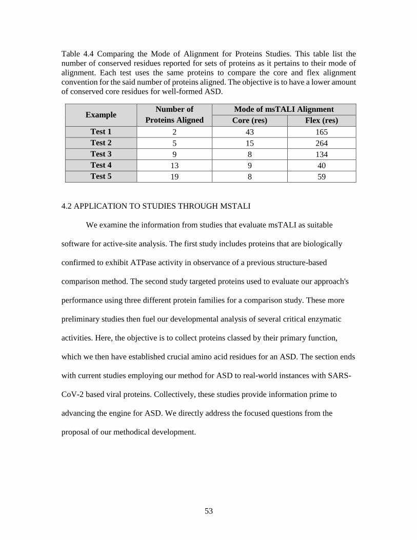
53

Table 4.4 Comparing the Mode of Alignment for Proteins Studies. This table list the

number of conserved residues reported for sets of proteins as it pertains to their mode of

alignment. Each test uses the same proteins to compare the core and flex alignment

convention for the said number of proteins aligned. The objective is to have a lower amount

of conserved core residues for well-formed ASD.

Example Number of

Proteins Aligned

Mode of msTALI Alignment

Core (res) Flex (res)

Test 1 2 43 165

Test 2 5 15 264

Test 3 9 8 134

Test 4 13 9 40

Test 5 19 8 59

4.2 APPLICATION TO STUDIES THROUGH MSTALI

We examine the information from studies that evaluate msTALI as suitable

software for active-site analysis. The first study includes proteins that are biologically

confirmed to exhibit ATPase activity in observance of a previous structure-based

comparison method. The second study targeted proteins used to evaluate our approach's

performance using three different protein families for a comparison study. These more

preliminary studies then fuel our developmental analysis of several critical enzymatic

activities. Here, the objective is to collect proteins classed by their primary function,

which we then have established crucial amino acid residues for an ASD. The section ends

with current studies employing our method for ASD to real-world instances with SARS-

CoV-2 based viral proteins. Collectively, these studies provide information prime to

advancing the engine for ASD. We directly address the focused questions from the

proposal of our methodical development.

54

4.2.1 Utility of ATPase Study

Our first structure-based study for active-sites relied on the analysis of 19 proteins

with certain ATPase activity. The basis for selecting these proteins relied on three

contributing factors: previous work for comparison purposes, structural diversity, and

complexity of the problem. These 19 proteins were subject to an earlier analysis using

Continuous Optimization (CO) [8] and Molecular Local Surface Comparison (MolLoc)

[33].

Analysis of ATPase proteins is compelling in two additional aspects; protein

dissimilarity and ATP's structural flexibility as a substrate. The diversity of proteins that

exhibit ATPase activity renders this problem particularly challenging and meaningful to

address. Table 4.5 lists the 19 target proteins with some of their binding properties.

Column two describes the organisms associated with each protein and highlights many

organisms, ranging from wild boar to human flu. Further, columns three, four, and five

highlight diversity in the residue length, ligand, and metal cofactors associated with each

protein, respectively. There is no single protein described by having a single ligand

interaction; in fact, some have as many as four, and cofactors range from Sulfate to

Lutetium. Structural diversity among these 19 proteins also constitutes a unique feature

of this problem. As mentioned, we also highlight some of the structural properties of the

target proteins. The sixth column shows the difference in C.A.T.H. classification [25]

even. This, in turn, describes variation in chain and domain characteristics for each

protein. Some proteins are primarily helical, others beta-strand, and others mixtures of

both; Table 4.6 provides cartoon rendering of these 19 proteins to highlight their

structural diversity further.

55

The Structural diversity of these proteins while maintaining primary ATPase

activity is central to our study. This problem's difficulty affords analysis descriptive

enough to convey what our msTALI system can withstand and what potential anomalies

manifest when applying to ASD. Here, we grasped additional insight into the sensitivity

to incorporate when aligning multiple proteins for ASD. The challenges faced by

studying ATPase activity pioneered our understanding of managing a grouping strategy.

They proved tonal for the simultaneous and subsequent alignments performed for the

successful aggregation of conserved residues. We addressed target protein use with

greater detail in section 4.1.

Our application of msTALI for active-site identification successfully identified a

motif characteristic of ATPase activity. Additionally, we report the successful

identification for the ATPase active-site complex documented for 1ATP-E while

adhering to our phylogenetic analysis conventions. We specifically address how eight

residues obtained from the study's simultaneous alignment are leading-edge for building

the overall ASD. Figure 4.3 displays our msTALI identified active-site, and the

biologically confirmed active-site for the protein 1ATP-E. Figure 4.3A highlights the

biologically confirmed active-site and Figure 4.3B the conserved core residues we

produce. Residues in common are shown in Figure 4.3C. Figure 4.3D shows the

superimposed relationship of A, B, and C.

Further, we attained far superior conserved regions in comparison to CO and

MolLoc [32]. Also highlighted is our reporting, which is consistent with amino acid

residues instead of atom-based representation. This is more consistent with

documentation. It reduces computational rigor concerning atom-to-residues conversions

56

with geometric constraints while valuing that residues conserved occupy more physical

space for proteins. All of which are useful for evaluating studies and for aiming to build a

streamlined standard approach.

Table 4.5 ATPase Target Protein Overview. We describe Target proteins by the organism,

the ligands, and metal complexes they bind. *1.Methanocaldococcus Jannaschii

*2.Thermococcus Kodakarensis

PROTEIN ORGANISM LIGANDS METALS

1A82 E. Coli mutant ATP, DNN MG

1ATP-E House Mouse ATP MN

1E2Q Human TMPK ATP, TMP MG

1F9A-C M. Jannaschii*1 ATP MG

1JJV Human Flu ATP, SO4 HG

1KP2-A E. Coli ATP, GAI, PO4 NONE

1MJH-A M. Jannaschii*1 ATP MN

1AYL Plant E. Coli ATP, OXL MG

1B8A-A T. K.*2 ATP MN

1CSN Fission Yeast ATP, SO4 MG

1E8X-A Wild Boar ATP LU

1G5T Salmonella ATP MG

1GN8-A E. Coli ATP, SO4 MN

1HCK Human ATP MG

1J7K Thermotoga

Maritima ATP, ACT, HEZ CO

1KAY Cow ATP MG, CL, K

1NSF Chinese Hamster ATP MG

1YAG Human ATP, SO4 MG

1PHK European Rabbit ATP MN

57

Table 4.6 Secondary Structure for ATPase Target Proteins. Here includes the cartoon

rendering of the 19 target proteins, all of which are confirmed to have ATPase binding

activity. Further, the table illustrates the diversity in structural components for each protein.

1ATP-E 1AYL 1B8A-A 1A82

1E2Q 1CSN 1E8X-A 1F94-C

1G5T 1GN8-A 1HCK 1J7K

1JJV 1KAY 1KP2-A 1MJH-A

1NSF 1PHK 1YAG

58

Figure 4.3 The active-site for 1ATP-E. A. The confirmed residues for ATP

binding as documented from the PDB. B. Illustrates conserved core residues

responsible for ATP binding as output returned from msTALI. C. The

overlapping areas common from representations A and B. D. The active-sites

are rendered in respect to one another.

59

4.2.2 Utility of Fold Families for Evaluation

We've established that our approach to ASD produced meaningful results. Better

again, our preliminary studies applied a difficult, more flexible functionality in ATPase

activity. In turn, the evaluation of the method is essential. Here we use proteins with

more similar structural composition and functionalities to discuss accuracy. We note that

a high structural similarity amongst the set constitutes a different degree of difficulty.

The high similarity between protein structures lends to more conserved residues and a

higher possibility for overfitting. Overfitting is not suitable for the overall ASD.

However, we accept the readily available documentation to evaluate accuracy. We

simply apply our thresholds for returned residues (based on protein length) to disregard

non-important features for ASD to address the high structural similarity. Further, with

prevalent documentation and details from the previous studies, we verify evaluation in a

base case format.

Our structure-based identification of active-sites relied on the analysis of 15

proteins. Selected based on previous reports and method comparison [18]. The proteins

are classified into three families of enzymatic activities: G proteins family in P-loop

folds, PYP-like family in Profilin-like folds, and FAD-linked reductases family

FAD/NAD(P)-binding folds. The G-domain and Ras superfamily are well known [34],

profilin is widely studied for cellular activity [35], and the same holds for analysis of

FAD based proteins [36]. Our evaluation starts with assessing our target set's

relationship since we know that we are using a lucrative amount of targets for ASD. In

Figure 4.4, we illustrate the structural similarity across each fold family. Our structural

alignments through msTALI are supported in P-loop folds, Profilin-like folds, and

60

FAD/NAD(P)-binding folds, with 173, 119, and 495 conserved residues with backbone

RMSD values of 1.30, 0.43, and 0.69 angstroms, respectively. Considering each

corresponding protein fold family's average length is roughly 184, 124, and 505 amino

acids long; our proteins are indeed structurally similar. In any of these cases, the

structural conservation isn't sensitive enough as we return between roughly 94 – 98

percent of the structure. To this point, we employ our technique of aligning all of the

proteins together simultaneously, not exclusively by their fold family. We then use the

subsequent alignments in conjunction with our simultaneous conserved regions to

address ASD and our evaluation focus. There isn't an all-inclusive analysis metric for

ASD, but several adapted models to reference documentation available in databases of

interest. We use PDB. For our comparison, we use two factors; precision and recall, as

previously reported [18]. We employ Eq. (2) to quantify precision. Where precision is a

percentage comparison of residues returned, consistent with confirmed documented

findings.

𝑃𝑟𝑒𝑐𝑖𝑠𝑖𝑜𝑛 = 𝐴𝑆𝑚𝐶

𝐴𝑆𝑚𝑀⁄ (2)

Here, ASm refers to the actual number of active-sites obtained from the method; in

our case msTALI. The subscript, C denotes returned active-sites from the technique that

are confirmed as active-sites. The subscript M denotes actives-sites that are simply

measured and outputted by the method. Secondly, we use Eq. (3) to quantify recall,

which incorporates Eq. (4) to obtain our value. The recall is used to track the overall

amount of active-sites discovered outright through our method.

𝑅𝑒𝑐𝑎𝑙𝑙 = 𝑀𝑆𝑝 − 𝐸𝑟𝑟𝑜𝑟 𝑆𝑐𝑜𝑟𝑒 (3)

𝐸𝑟𝑟𝑜𝑟 𝑆𝑐𝑜𝑟𝑒 = (𝐴𝑆𝑚𝑀− 𝐴𝑆𝑚𝐶)

𝐴𝑆𝑔𝐶∗ 𝜀 (4)

61

Here, MSp refers to the maximum number of active-sites that can be recovered,

total coverage being 100 percent. We define our error score as the penalty evaluated from

our precision. Whereby, the 𝜀 multiplication addresses how great of a penalty factor we

allot. The value 𝐴𝑆𝑔𝐶 is the represented number of confirmed active-sites documented.

The reported evaluation is in Figure 4.5. We list the G proteins family in P-loop

folds, PYP-like family in Profilin-like folds, and FAD-linked reductases family in

FAD/NAD(P)-binding folds, and highlight them respectively; purple, green, and red. As

mentioned, we compare our evaluation to BsFinder, and several others by association

based the precision and recall. Before looking forward, we note the size of the proteins.

Our largest proteins are documented as not exceeding 4000 atoms in length, and the

largest recorded active-site size does not exceed 260 atoms. Henceforth, any reported

values that exceed these thresholds use a representation subject to overfitting.

We declare that there are inconsistencies with reporting. Approaches do not have

a unified reporting convention. Some use atomic representations as opposed to the

amino-acid residue. Our aim is a more applicable reporting evaluation. We disambiguate

any atomic and locational constraints by using purely documented residues for each

protein. Figure 4.5 the column heading with "Numbers" for each method (columns six

and eight) demonstrates how such inconsistencies result in drastically different charting

for the number of found active-sites. The results at first glance could be misleading.

Consequently, we translate our protein size to the number of atoms for both the

protein and its active-site size. Columns three and five of Figure 4.5 report the confirmed

corresponding length in atoms. Our initial reporting in amino acid length (residues) is still

shown in columns two and four. It's how we document the particular instances where

62

msTALI stands out to BsFinder; since they are comparable at first glance. However, all

of our results – msTALI for ASD – fit within reasonable bound of the confirmed sizes for

each protein (whether verified total length or confirmed active-site size).

Discussing precision and recall is straightforward once conserved residues are

reported and compared to the confirmed active-sites. Through comparison, we use the

conserved residues that are found and confirmed for evaluation. From Figure 4.5, the

seventh column first lists the precision value we mentioned, followed by a second

number, the calculated recall. We report our results alongside those of BsFinder [18],

highlighting our instances of outperformance. We've marked values yellow for precision

and cyan for recall when msTALI is superior. Values colored grey highlight msTALI

results less than that of BsFinder but by no more than five percent. The nuances that arise

from evaluating this particular target set of proteins are addressed directly [31]. Still, we

acknowledge the drawbacks witnessed with some exampled proteins or fold families

within the target set. It would appear that our method is relatively comparable; however,

our approach is ahead 73% of the time for this study.

Moreover, our results are consistent with a maintainable point of reference in

PDB. Overall, when comparing the initial accuracy of our method, we fair higher across

the board. This remains the case, even when a broader set of proteins is studied. Our

averaged precision is 37%, and our recall is 84%, as reported in Table 4.7. All of the

aforementioned supports our approach lucrative for ASD.

63

Figure 4.4 The Super Imposition of Protein Fold Families. A. Superimposed structures for Proteins 1A2B (green),

1CXZ (orange), 1DPF (grey), 1FTN (red), and 1SIC (blue) from the G proteins family in P-loop folds. B. Proteins

1D7E (green), 1F9I (orange), 1KOU (grey), 1NWZ (red), and 2PHY (blue) form the PYP-like family in Profilin-like

folds. C. Proteins 1B4V (green), 1B8S (orange), 1COY (grey), 1IJH (red), and 3COX (blue) from the FAD-linked

reductases family in FAD/NAD(P)-binding folds.

.

64

Figure 4.5 The Confirmed Protein Information needed for Precision and Recall. Using PDB we’ve listed the length by

amino acid residue and the length in atoms. We then compare the precision and recall for msTALI and BsFinder. Results

from BsFinder were previously reported [16]. With *a. the first number is the number of output sites reported by the

program (conserved regions in our case), the second number is confirmed sites from the program. For *b. and *c. the first

number is the precision value (%), the second number is the recall value (%) for both msTALI and BsFinder approaches

respectively. Reporting by residues is consistent with documentation.

65

Table 4.7 Program Evaluation Comparison on Fold Families. This table includes a

comparison of four discussed programs as reported from a previous study observing 55

sets of proteins (our results for msTALI are set alongside)[18].

Program Precision Recall

msTALI 37% 84%

BsFinder 34% 82%

SiteEngine 21% 47%

SuMo 11% 25%

pdbFun 15% 11%

To complete our evaluation study, we illustrate the conserved core region by

simultaneously aligning all 15 proteins; we then provide an example from each fold

family. This establishes the foundation of our ASD and is pictured in Figure 4.6. Each

illustration serves as an abstraction of the overall ASD for the proteins highlighted.

Figure 4.6A illustrates the conserved region for protein 1A2B, Figure 4.6B does the same

but for protein 1D7E, and Figure 4.6C depicts protein 1B4V. Figure 4.6D is a

superimposed surface representation of the conserved core regions across A, B, and C

and exemplifies structural similarity. To highlight the similarities further, Figure 4.6E

renders the same motif for secondary structure. The depicted conserved core regions from

msTALI are consistent across all target proteins. Confirmed active-site regions are

surface accessible or at the center of cavity/ cleft locations respective to a protein family

and are located at the coil, non-structure, or turn and bend regions at the beginning of the

alpha-helical region of each target proteins conserved residues [34][35][36]. We observe

that our simultaneous alignment on all 15 proteins yields precise results, characterizes

motifs common to all the proteins observed, and endorses the validity in active-site

bindings unique to each protein.

66

Figure 4.6 The Conserved Core Regions. Each example is observable from three proteins, one from each fold

family under the all-inclusive simultaneous alignment. A. The conserved core residues for protein 1A2B as

obtained from msTALI. B. Comparative results for protein 1D7E. C. Comparative results for protein 1B4V. D.

Illustrates the superimposed regions from A to C. E. Depicts the secondary structural area from D.

67

Our evaluation study established comparison characteristics for our overall

approach. We develop a plan for documenting active-sites by visualizing the top-ranking

protein from studied target sets. The framework is then applicable to future studies. The

simultaneous alignment relation to active-sites is convincing alone. However, the

inconsistencies across approaches make it difficult to characterize a holistic mechanism

for identification evaluation. We assert the continual use of PDB for validating

documented proteins. Again, we note that our method is competitive and applicable to

broader ASD studies for multiple enzymatic activities.

4.2.3 Focused Study of Proteins

Our underlying hypothesis states that when the structure-sequence alignment of

multiple proteins with common function is performed, we will reveal the conserved

regions, which must contain the active-site and motifs salient to functionality; this indeed

holds as our primary aim is to successfully qualify several regions directly related to our

claim for a selected group of enzymatic activities. Our methodology stands out since it

doesn't require the computational and often exhaustive exploration of substrate

conformations seen with docking techniques. Further, experimental descriptions are

expensive and time-consuming. We move to an ASD description that expands beyond

our preliminary studies.

Our protein classes include AMP, ATP, FAD, FMN, Glucose, Heme, Hydrolase,

NAD, Phosphate, and Steroid functioning proteins. Studies performed on these functional

classes have had success, stress the importance/ relevancy of each functional group, and

even test the variation in shape locals' binding [20]. We review each class of proteins in

this section for our primary findings; they also advance our web-app development

68

methodology. However, considering the complexity of the problems faced with ASD, we

have two ways to assess our results in this section. First, we compare our results to other

methods. Second, we highlight components from each class of proteins.

4.2.3A Summary Comparison of ASD with msTALI to Accepted Approaches

Our initial approach to evaluation explored the precision and recall of our method.

Remember that precision virtually reports the percentage of results that are indeed

lucrative. The recall is the number of active-sites that are recoverable provided we assess

errors. In each metric, we are testing our approach for accuracy based on available

documentation. Accepted practices have fared, having precision below thirty-five percent

and recall values roughly eighty percent [18].

Further, some instances have acceptably exercised accuracies as low as eleven

percent. We detailed the specifics of observed methods in Table 4.7. To this point, our

primary results are aggregated together in Table 4.8, where we report each class of

proteins precision and recall using our method. Notably, our precision values are all

upward of thirty-five percent. When compared, our recall values outweigh established

approaches threefold, even in worst-case examples. From Table 4.8, our first column

highlights the confirmed function for each study's set of proteins. We've included our

summarized results from preliminary evaluation studies detailed in section 4.2.2. We

examined upward of ten classes of proteins for validation. We summarize our results in

the last row of the table. We express the total precision and recall as an average across

sets. Despite our findings exceeding standards, there is still room for improvement.

However, many emerging ideologies that expand understanding are reaching ceilings in

advancement. Consequently, the current focus in active-site discoveries is equally vested

69

in standardizing the evaluation of approaches [29]. To this point, we resort to

representing results for our protein studies visually.

Table 4.8 The Primary Precision and Recall for Our Approach. Each class of studied

proteins is reported and averaged for a total representation of performance on ASD.

CLASS PRECISION RECALL

AMP 36.2 93.5

ATP 57.0 94.6

FAD 37.3 96.4

FMN 70.7 95.7

GLC 38.8 86.6

HEM 48.5 95.8

Hydrolase 36.5 95.8

NAD 56.5 90.6

PO4 48.2 94.0

Steroid 39.9 69.3

G(3 folds) 37.0 84.0

Across All Activities 46.0 90.1

4.2.3B Composite Results Highlighted Based on Enzymatic Activity

Evaluation of computational methods aiming to identify active-sites is disjoint.

The lack of standards stems from ranging approaches, intricacies of the problem in

general, and the direct means for comparing results. We have reported our results for

ASD with an average precision of 46.0% and recall of 90.1%. Still, several of our studied

proteins do not have a standard for evaluation or another computational approach for

comparison. Further, if a method is available, it is not sure to adhere to annotations from

the PDB or any other formal repositories. This section includes additional context for

processing our precision and recall. It is notably beneficial to relate to how our results

engage implementation since we have reported how our approach fares better for our

studies. More so, this section highlights our studies' results based on visually showing

70

regions we assert are exemplary to the ASD for the target classes of proteins. We

visualize motifs as a collective and highlight individual protein from our focused studies.

From our summary, we establish that our average precision is 46.0% and recall is

90.1%. Additionally, even with values higher than those having established use, visually

rendering results serve most beneficial for well-rounded representation. Still, we must

provide details that aid in interpreting the success of our method. We include the receiver

operating characteristic (ROC) curve [37] for our approach and other details for more

context. For the focused study, 4,380 protein residues were significantly recognized, and

2,125 of these residues were confirmed active-sites. This ratio is just upward of our

reported average precision. We also stress that several of the false positives are beneficial

to annotation and provide insight to function. The full acknowledgment for significant

confirmed residues is noteworthy. With our ASD, we suggest recommendations that

serve single protein evaluation differently. For example, we report a precision of 46%,

but, again, our collective success ratio from above is nearly 50%. Understand that an

individual protein has a different ASD than others in its class but often share several

signatures. Essentially, our observations are balanced by class and unbalanced when

considering the proteins that make them.

On average, for a span of 332 observations, we obtain an F-measure of 0.53 from

precision and recall. Our F-measure is lucrative provided the problem. Moreover, when

transitioning to contextual evaluations for proteins from a class, roughly 230 of the

observations are classified as confirmed active-sites. Figure 4.7 shows the ROC curve for

our method of ASD, based on the reported residues from our focused study. Graphed in

the figure, we map our sensitivity and the complement of our specificity.

71

Figure 4.7 Active-Site Identification ROC curve. The graphed ROC curve for our method of

ASD provides details related to the number of active-sites found for proteins within a study.

This analysis further alludes to the number of times proteins should undergo alignment for ASD

before compromising our reporting. Our Green marked data point is our recommended standard,

and the yellow point is within a manageable range.

72

Together, the two graphed metrics convey the tradeoff between false-positive and true-

positive rates. We have highlighted two data points, one green, and one yellow, and use

them to directly explain what comes from Figure 4.7. Our green point has a sensitivity of

0.41 and a false-positive rate of 0.20. The yellow data point has a sensitivity of 0.54 and a

false-positive rate of 0.35.

We highlight these regions because they most support our methodology. The

highlighted regions from our ROC curve coincide with the observable conserved regions

that result from a msTALI alignment. Our green point informs us that when twelve

conserved residues are returned, we will most likely have a successful ASD for a studied

protein. Our yellow point represents ten conserved residues (we point this out since the

grouping does not diminish results too much). Analysis with the ROC curve affects our

approach by establishing the standard for simultaneous and subset alignments. Directly,

our recommendation is four sets of alignments. Our green point supports this with a

general acceptance at 12 conserved residues. We observed complete correctness for the

classification of these observations as active-sites/ functionally significant were all

present.

Further, with 12 residues run four times, based on alignment, we maintain our

Threshold. The overall Threshold is 55 residues, and with 48 residues, we do not exceed

it. Anecdotally, we could use values below the recommended cutoff (green point), but

those instances are best suited for exceptional cases where the targeted class of proteins is

well defined. The use of precision, recall, the ROC curve, and evaluation in general all

provide contributory insight for our approach. However, we still stress rendering proteins

to provide first-hand examples for the conserved regions we associate with ASD.

73

Our focused study examines ten classes of proteins. A protein from each class is

selected to expand our report. We also detail findings for our top ranking functional class

(FMN functioning). All depicted proteins rank amongst the top three results from their

respective studies. This reporting strategy calls attention to findings while stimulating

observations made through validation from the PDB annotations. We first describe the

recovered ASD for FMN. We then list the collective regions in Table 4.9, along with the

sequence information. Notably, we list the amino acid sequence only for our prevalent

findings in all the functional group proteins. To conclude our focused report, we picture

the corresponding visual representation for each protein.

FMN functioning proteins rank highest amongst the ten function classes. Several

responses suitably describe why one studied class evaluates higher than another.

However, the intermingling details become overbearing for our primary aim; as expected,

there are anomalies within each set, which do not impact the larger theme and fall outside

the scope of our focus. FMN (Flavin mononucleotide), as many targeted functional

classes, is very prevalent in biological interaction. Specifically, FMN has involvement

with metabolism, and its believed interactions play a role in the electron–transfer

pathway [38]. We notice that protein 1FLM from our FMN study was evaluated

exceptionally well. Reasons attributing to 1FLM being standout are primarily its size and

relationships. 1FLM is the smallest of FMN binding proteins; it is 122 residues in length

and further binds only with FMN. Figure 4.8 highlights the ASD we characterize with our

approach. The regions highlighted red are confirmed active-site residues that are contact

regions. The blue is our found overlapping regions, which consistently fit –

74

Figure 4.8 Highlighting the ASD for Protein 1FLM. We use red to outline confirmed

active-sites residues from PDB. Blue are overlapping regions consistent with our

findings. Yellow regions are prevalent in all proteins from the corresponding functional

class.

75

with the confirmed active-site. The yellow corresponds to residues within the protein

1FLM that are also structurally present in all the studied FMN proteins.

With 1FLM, we have afforded a complete protein level description for our

focused study of proteins. Further, our ASD includes both active-site and functionally

significant residues. Overlapping regions directly facilitate function. Most notably, by

serving as the structural clamp-like feature that fosters the hold at the docking location.

These physical interactions are supported by the hydrophobic and hydrophilic

interactions at the site, as well [38]. Again, we expand these results to the FMN class, use

the same convention across all classes, and expound on how they link to composite

results.

Results illustrated in Table 4.10 directly map regions consistent with reported

residues in PDB. In other words, each structural representation – colored blue – is an

overlapping region constant to our approach. Yellow areas are highly conserved residues

indicative of all the proteins studied from their respective class. It is salient to mention

the colored areas for two reasons. First, the overlapping residues, assure that our

identified regions are functionally significant. Second, yellow regions are holistic and

stress the studied class's relationship and any homologous protein moving forward.

Both points are unique to our approach and have impactful implications. For each

component of our focused study, we have found structures critical to function. We see

that regions are sometimes just as well-formed as they are dynamic. By, connecting

proteins based on their functional relationships, we can rapidly approach current issues.

This serves as beneficial for the annotation and drug design of any protein of interest for

real-world applications.

76

Table 4.9 Annotation for Focused Study Proteins. From our focused study, we outline the ten top-ranking proteins for each group. The

confirmed conserved residues are confirmed as causal to function from PDB annotation. They are also based on proximal relevance.

Standard functional listings report residues that are present in all studied proteins for the respective class. We list the sequence

information for these regions. Highlighted residues are colored blue and yellow, respectively, and visible in Table 4.10.

Protein Confirmed Conserved Residues for ASD (blue) Common Functional

(yellow)

Common Functional

Sequence

1CT9 1, 2, 3, 4, 5, 6, 7, 40, 41, 42, 43, 44, 45, 46, 47, 48,

49, 50, 51, 52, 70, 71, 72, 73, 74, 75, 148, 149,

1, 39, 40, 41, 42, 43, 44, 45,

46

A A S D N A I L A

1E2Q 18, 19, 20, 21, 22, 23, 24, 45, 67, 75, 76, 77, 78 79

102, 103, 104, 105, 107, 108, 154

17, 18, 19, 20, 22, 23, 24,

25

V D R A K S T Q

1JR8-B 8, 9, 10, 12, 13, 20, 21, 22, 23, 24, 25, 45, 46, 47,

48, 49, 50, 51, 54, 55, 58, 61, 62, 67, 78, 79, 80,

81, 82, 83, 84, 85, 86, 87, 88, 89, 90, 91, 92, 100,

45, 46, 47, 48, 49, 50, 51,

54, 55, 58 Y A E L Y P C C S F

1FLM 12, 13, 14, 15, 16, 17, 18, 19, 51, 52, 53, 54, 55,

56, 57, 58, 59,

12, 13, 14, 15, 16, 17, 18,

19

N E G V V A I A

4R2B 14, 18, 20, 30, 31, 32, 33, 34, 35, 36, 37, 38, 39,

40, 41, 42, 43, 149, 150

30, 31, 32, 33, 34, 35, 36,

37

L E K K G I S W

1QPA-B 34, 35, 36, 37, 38, 39, 40, 41, 42, 43, 44, 45, 46,

47, 48, 49, 50, 51, 278, 279, 283, 287, 288, 289

38, 39, 40, 44, 46 E A H R V

1V2G 9, 18, 19, 20, 21, 22, 25, 26, 27, 28 18, 19, 20, 21, 22, 25, 26,

27, 28

S A S A A A L L N

1OG3 5, 66, 67, 81, 83, 84, 92, 93, 94, 95, 125, 126, 127,

128, 129, 130, 131, 132, 133, 144, 189, 193, 195

27, 31, 32, 37, 38, 39 E L F N M

1DAK 10, 11, 12, 13, 14, 15, 16, 17, 32, 33, 34, 35, 36,

37, 50, 51, 78, 79, 80, 81, 83, 152, 153, 154,209

32, 33, 34, 35, 36, 37 R T A G Y K

1E3R-B 13, 14, 16, 17, 18, 19, 20, 21, 22, 98, 99, 100, 101,

105, 111, 119, 120

11, 12, 13, 16, 17, 18, 19,

20, 21, 22, 70, 105, 111,

112

G L M A R Y I E L V D

V L M G R

77

Table 4.10 The Prominent Protein Features for the ASD on Focused Studies. Images A. through J. depict conserved residues obtained

from our approach that is also confirmed binding regions in PDB (blue). We find that Yellow regions are in each protein within a set.

A. 1CT9 B. 1E2Q

AMP ATP

C. 1JR8-B

FAD FMN

D. 1FLM E. 4R2B

GLC

F. 1QPA-B

Heme

e

H. 1OG3

NAD

G. 1V2G I. 1DAK

PO4

J. 1E3R-B

Ster. Hydr.

78

4.2.4 Current Applications of ASD Through msTALI

The utility of msTALI for active-site identification and, more specifically, the

ASD of proteins are primarily based on researched studies. The studies, as mentioned,

typically have some known components based on documentation. All of which is useful

for testing and verifying our aim. Evaluation is essential, and our accuracy ensures that

our method is sustainable. Nonetheless, the invaluable task is applying our newly

developed method on novel protein structures, current matters worth analysis, and any

combination of those fitting to the times. Within this section, we outline two applications

of ASD. The first takes advantage of several techniques observing a novel protein

structure, and we focus on the contributions of msTALI. The second application is related

to the pressing issues relating to COVID-19. In both cases, annotation is critical, and we

use these examples to strengthen our methodology's reach to real-world practice. The

importance of protein functional discussions is relevant. From annotation to drug design,

computational methods are directly beneficial to expanding the field's common core

principles.

4.2.4A Nonstructural Protein Annotation for NSP1 in SARS-CoV

Real-world application for our approach is inescapable. We have verified our

results through comparison studies and move forward with advancements observing less

annotated structures. Our first example here is conducted on nonstructural protein 1

(NSP1). We observe NSP1 due to its cleaving characteristics from SARS-CoV studies.

NSP1 is of the nsp family of proteins and the first to be translated [39]. It causes severe

translational shutdown of host proteins from host mRNAs and, in turn, suppresses host

gene expression. Additionally, its structural makeup has three regions, two unstructured –

79

domains, and the other is structurally well-defined. Further description lends to

cataloging the 180 residue makeup. Residues 1 – 12 and 127 – 180 are unstructured, and

13 – 126 are structurally well-defined [30]. Provided that genomic information is

available, we still need to explore the functional qualities. Consequently, we rally our

ASD approach for novel developments with supporting computational approaches

investigating regions of interest for NSP1 [30].

ASD for NSP1 is a lucrative pursuit since the structure-function relationship has

direct implications for COVID-19. Other studies for COVID-19 focused on spike

proteins binding to the lung cell receptor ACE-2 [40]. Here, our relationship of NSP1

with SARS-CoV widens our understanding of SARS-CoV-2 (COVID-19) based on

homology. We use our methodology to study NSP1's disordered regions in a manner that

proves challenging for traditional methods. We apply our method and integrate it with

other computational approaches and experimental validation for a well-rounded

collaborative markup for function. Through laboratory-based experiments, two regions of

NSP1 were explored and shown to alter its ability to shut down host gene expression

[30]. We believe that these mutations' implications are structure-functionally significant

for the protein and expandable; we show the potential regions in Table 4.11. For a

complete consideration of NSP1's function, we corroborated our findings for ASD with

the structural modeling of I-TASSER [41] and deep mining of the PDB using PDBMine

[42]; collectively, this affords a reliable deciphering of NSP1 in a timely manner that

escapes traditional applications.

80

Table 4.11 Gene Expression Inhibiting Residues of Interest. Laboratory confirmed

mutations that inhibit host gene expression by amplifying NSP1’s function.

Gene Expression Inhibited by 150-450%

E55R, E57R, K58E, G59R

R73E, D75R, L77A, S78E, N80G

Again, we focus on our direct ASD results as active-site studies are also essential

for expressing proteins' functional operation. Our contribution upholds the methodical

convention described throughout section 4.1. These controls include the number of

targets and diversity in structure while maintaining functional relevance and binding to

NSP1. Table 4.12 highlights our preliminary target set for alignment. We list their length

in residues and C.A.T.H. classification (if available) to ensure our approach is self-

contained. Our standards are maintained, and our criterion is mobilized for ASD.

Table 4.12 Preliminary Protein List Related to NSP1 Functional Activity. Here we

supply the list of proteins with related functional activity to NSP. They were used with

msTALI for ASD.

PDB-ID Size CATH

1HUS 155 1.10.455.10

1IQV 218 1.10.455.10

1VI6 208 3.40.50.10490

1QKH 92 3.30.860.10

1QXF 66 2.20.25.100

1RIP 81 2.40.50.140

1RSS 151 1.10.455.10

2FKX 88 1.10.287.10

2MEW 82 3.30.70.600

3BN0 112 3.30.1320.10

4BSZ 244 3.30.300.20| 1.25.40.20|

3.30.1140.32

6G04 156 NA

NSP1 180 NA

81

With the following, we address the resulting annotations obtained from using our

msTALI based method for ASD. The results of the alignment of the proteins listed in

Table 4.12 are shown in Figure 4.9. In this figure, each region of the protein is marked by

its residue number. Higher scores correspond to regions of the protein that are conserved

and deemed significant for our typical ASD. We list peaks in Table 4.13, where each

conserved region is named by the residues it spans, and described the degree of surface

accessibility. There are two particularly interesting observations. The first indicates the

importance of region 73 – 80, one of the implicated functional regions of NSP1. The

second observation relates to the near-complete absence of any reported significance for

the region 55 – 59. This is highly related to the structural similarities amongst the target

set for ASD. The accompanying proteins have relevant binding properties. Consequently,

region 73 – 80 is more likely the initial binding site to the rRNA complex. Further, it can

be hypothesized that the additional regions (1, 2, and 4 - Table 4.13) are requisite

supporting regions that facilitate the docking process at residues 74 – 83.

Table 4.13 Surface Accessibility for Conserved Regions of NSP1. The conserved regions

across the alignment of NSP1 with the remaining twelve proteins of the target set. All

proteins have functions related to that of NSP1.

Name Range Surface Accessibility

Region 1 7-15 Partial surface exposure

Region 2 22-29 Partial surface exposure

Region 3 74-83 Complete surface exposure

Region 4 139-146 Minimal surface exposure

Our method's significant regions coincide with both the focused regions and

additional residues that we reliably advocate as functional facilitators. The consistent

backings for residues 73 – 83 are promising, and the others are beneficial to our overall

ASD based on structural similarities. We summarize the results by rendering the protein –

82

structure for Wild-type NSP1 in Figure 4.10. The established regions outlined in Table

4.13 and Figure 4.9 are colored green. The mutation/ focused regions outlined in Table

4.11 are colored red. We then highlight the overlap of green and red regions, blue.

Residues highlighted blue (73 – 83) consistently stand and are critical binding sites in the

ribosomal binding function. We reiterate our results exclude the region 55-60; however,

with additional observation, a region emerges with supplementary potential. The yellow

region in Figure 4.10 is added to our markup for this reason. We discuss its proximal

significance further in section 4.2.4B. Collectively, the rendering of NSP1 is the

culmination of our observations. Proximal locations join our computational descriptions

[30] for a reliable annotation. We see that despite divergent mechanisms for function, our

ASD includes functionally supportive regions for biochemical interaction. Findings are

all well suited as a foundation for COVID-19 studies based on homology [39].

4.2.4B Application of The msTALI ASD for COVID-19

Transitioning from important novel structures, we engage in establishing

templating approaches for a known protein, based on its relational lineage and despite its

unclear description for its active-site relationship. We focus on structure 6LU7 for our

COVID-19 study, and we link its importance to previous viral outbreaks. We link its

impact to severe acute respiratory syndrome (SARS). The SARS virus sparked interest in

the early 2000s as its outbreak reached the masses. To date, the coronavirus named

COVID-19 has directly affected the mode of living and interactions at a global capacity

and for the overwhelming majority. The current understanding of the coronavirus's

lineage suggests viral flexibility that is also problematic for the future.

83

Figure 4.9 The msTALI conservation score for SARS-CoV-1 NSP1 protein as reported with the other proteins from the target set. A

higher score is an indication of a more significant conserved region.

84

Figure 4.10 The Visual Rendering of Wild-type NSP1. We represent and highlight observable regions for SARS-CoV-1 NSP1 resulting

from our ASD. Highlighted protein residues correspond with our highest conserved core results, experimental focused regions for

mutation, templated results, and the common residues between the conserved core and experimental regions. We color each region

green, red, yellow, and blue, respectively.

85

With such, the viral genome is readily studied and of interest. Further, even knowing that

the SARS and the coronavirus COVID-19 are RNA inhibiting, the specific gene products

are still relatively unknown, especially when describing function [43].

We apply our method of ASD to COVID-19 with an additional observation of the

following proteins: 1DIV, 1DK1, 2C3S, 2GHV, 3QOY, 5CWS, 5GQT, 5WRG, 6ACD,

6LU7, 6W02, 6Y2G, 6Y84, 7BTF, and NSP1. The selected list is built from continuing

our protein structure-to-function study on NSP1. Since there are details elusive to our

documentation of 6LU7 – our COVID-19 structure – we use additional available

resources. We incorporate our leading ASD description from simultaneous alignment

with our novel results and reference materials obtained from PDBsum [44] to build our

story for 6LU7. More specifically, we highlight relationships between the simultaneous

alignments of protein 7BTF and the NSP1, as mentioned earlier.

We observe seven residues across the proteins that are highly conserved. These

seven residues then become the basis for motif characteristics for each protein in the ASD

study. From Figure 4.11, the seven residues are plotted by residue location for each

protein. The peaks correspond to the conserved regions, and we see there is also proximal

similarity across the set. We highlight additional proteins of interest concerning 6LU7.

Graphs J, N, and O from Figure 4.11 are noteworthy because their proximal

similarity is also linked to documented regions of importance. With protein 7BTF ("N"),

all seven residues are confirmed active-sites, making it the best fit result for the initial

motif definition. The confirmation of residues alludes to the region's propensity to fit

directly for the overall target set for ASD and make it a reliable template for our focused

6LU7 graphed in J.

86

For NSP1 in O, we again observe conserved regions noted to facilitate its

function's initial steps. In these studies, regions once missed are more prominent [30].

Notably, the emergence of the supporting area is not direct. However, this is not

surprising as the presence of different host factors – RNA or Protein – affect the

supporting residues aiding the function for ASD. Particularly, we discuss the residues 50

– 54 highlighted yellow in Figure 4.10. Several established methods for active-site

identification group neighboring regions with the site. Base on proximity, the same is

acceptable for our mutation region at residues 55 – 59 [30] for NSP1. All residues are

within five amino acid locations of each other (spanning ten residues in total). Thus,

labeling the emergent region as functionally supportive is lucrative. Region 50 -54 is also

a beta-structured region connected to the nanostructured residues 55 – 59; we valuably

add them to the markup for ASD. Our observations now include several conserved

features that are adequately applicable to 6LU7.

4.2.4Bi Identifying Prominent Features in COVID-19 for ASD

There are well-documented structures, novel structures, and several that are

annotated far less despite being known and classified among our target proteins. We

reiterate this because it is causal to the templating concepts for our method verification.

COVID-19 is one of the less annotated proteins for function. However, we have an

understanding of its impact. Expressly, 6LU7 [45] – our studied COVID-19 structure – is

confirmed in PDB as having an active-site consisting of only two residues; this is small,

and roughly twenty percent of that size confirmed for 7BTF (our template/ reference for

ASD). Other mentioned residues for 6LU7 are referenced from PDBsum. These

annotations are ambiguous.

87

Figure 4.11 The msTALI Conservation Score for Templated Set. Proteins are alphabetically listed

A through O for proteins. Higher scores represent significantly conserved regions for each protein

based on residue location. Proteins of focus are highlighted green.

88

They are not labeled as active-site or functionally causal. Instead, they are said to come in

contact with ligands [44]. We initiate our analysis of 6LU7 using the complete

conservation score to disambiguate annotation. The complete score plots for ASD is in

Figure 4.12. The msTALI conservation score exhibits four primary peaks consistent with

our findings.

4.2.4Bii Critical Protein Residue Rendering for COVID-19

To visualize our charted conserved regions, we list the protein residues first. The

framework affords a relationship for regions we visualize for evaluation. We consider

both the confirmed active-site and documented highlighted residues to evaluate our

approach since the PDB confirmation is small. From Table 4.14, column two lists the

residues we obtain with our approach, column three confirms PDB annotation, and the

fourth outlines highlighted regions from PDBsum. Using our technique, we recognize

forty-nine residues. There are two from PDB [24] and twenty-one from PDBsum [44].

The reported comparison regions share thirty-two residues in common based on residue

number, threshold, and proximity [31]. We visualize these details to highlight their

potential causality to function. The visual representations are increasing interesting for

two reasons:

1. We can verify spatial locations for residues and identify residues for the overall

protein. These qualities can allude to the alleged role of residues. Which, in turn,

highlight functional classifications and provides well-formed ASD.

2. With the protein models, similarities between 6LU7 can 7BTF are more noteworthy.

The templating approach is supported and reinforces the range in methodology. We

directly assert that our ASD results are replicable for other functional interests.

89

Figure 4.12 The msTALI conservation score for protein 6LU7. Higher scores represent significantly conserved regions for each

protein based on residue location. The x-axis charts the amino acid residue numbers for said protein; corresponding scores are

plotted along the y-axis.

90

We address the first interest for visualization next, as it pertains directly to the

ASD for 6LU7. Our second interest is described in our next section since it relates to our

methodology and how similar strategies from our method apply for the community

response.

Table 4.14 Reporting Conserved Regions for Protein 6LU7. The residues obtained from

the msTALI ASD are reported first, followed by the PDB confirmed active-site, and then

notable regions are added from PDBsum reports.

Reported Protein Residue Numbers

Named Protein msTALI

ASD

PDB Active-Site

Conformation

PDBsum

Highlighted Regions

6LU7

9, 10, 11, 12, 13, 14,

15, 16, 17, 18, 19,

20, 21, 22, 23, 24,

25, 29, 30, 31, 32,

33, 96, 97, 98, 99,

100, 101, 102, 103,

104, 128, 132, 151,

152, 153, 158, 169,

171, 180, 184, 185,

186, 187, 188, 189,

190, 241, and 247

41, and 145 24, 25, 26, 41, 140,

141, 142, 143, 144,

145, 163 164, 165,

166, 168, 172 188,

189, 190, 191, and

192

Related to our first interest, Figure 4.13A and Figure 4.13C provide

corresponding representations for 6LU7. Figure 4.13B and Figure 4.13D are

corresponding representations for each other as well. In each case, we display the

secondary structural representation followed by a protein surface representation. Protein

residues highlighted green represent column two in Table 4.14, and residues highlighted

red and orange are columns three and four, respectively. Blue residues highlight

overlapping residues consistent with our findings and the documented/ referenced areas.

From a proximity/ spatial perspective, all highlighted regions surround the large

centralized cleft of the protein. The individual representations provide descriptive

91

observations. In comparing our results from Figure 4.13A with Figure 4.13B, our results

envelop the confirmed active-site. Figure 4.13B region highlighted orange, covers the

face of the cleft. Pictured in Figure 4.13C and Figure 4.13D, the confirmed as active-site

(red-marked) are primarily submerged within the cleft. The contact ligand representation

(orange) covers the cleft surface/ geographical area in Figure 4.13D, while our found

ASD locations (blue) highlight the borders/edges of the cleft. These details are essential

for motif characterization and further support surface accessible regions' functional

responsibility.

We maintain that having two residues declared for an active-site is limiting.

However, we also have the orange highlighted region from Figure 4.13B, which are far

more similar to our results. Using a templating approach with protein confirmed similar,

we can assert our ASD result as regions that aid function. Our ASD for 6LU7 conveys

more than highlighted structures that cup the cleft. The proximal significance has

resounding implications for the ASD. As we look further into the motif itself, structural

components display convincing evidence that residues' role facilitates the function; they

line the cleft, engulf the active-site, and are in surface accessible regions that can close

off access to the cleft as a whole.

4.2.4Biii ASD Motif Rendering for COVID-19

The proximal similarities are significant, and the functional implications are

intriguing. Closeness to the active-sites or any other protein residues deemed interesting

is directly observable and pragmatic. However, the relationships from our studied protein

set are less intuitive. The template reference is used as a framework establishing an ASD

signature for studied classes of proteins. To visualize these points, we focus now only on

92

the characteristics templated from 7BTF to 6LU7. In doing so, we show the noteworthy

features for the viral proteins of our target set. The visual representation of our ASD

moves forward our second interest. We evaluate our approach's effectiveness for 6LU7

and demonstrate our application as suitable for reshaping the means for addressing other

functional activity, whether for ASD annotation or insight.

In Figure 4.14, our rendering of the ASD for 6LU7 focuses on our motif's

structural aspects. We establish their similarities with our template structure and observe

significant and exhibited regions across all of the target proteins. First, we highlight the

primary residues from 6LU7 and 7BTF obtained from all targets' simultaneous

alignment. Residues 184 – 190 are colored purple for 6LU7 and directly correspond with

magenta-colored residues, 642 – 648 of protein 7BTF. This region is highly conserved.

This region is prevalent in all of our observed proteins; it describes the peaks from Figure

4.12. Additionally, the residues highlighted for 7BTF are confirmed active-site. We

establish the conservation and superimpose these regions in Figure 4.14, noting that their

non-secondary structure conforms, and is fitting to active-site descriptors.

From the comparison of our base region, other template fitting features become

prominent. We establish what is comparable and useful for both the ASD of 6LU7 and

any related functional examples. Protein 6LU7 is colored green, and 7BTF is colored

cyan. We discern two additional pairing regions that match the purple and magenta

described regions in Figure 4.14. The similarities are strikingly similar for the two

accompanying secondary-structure heavy areas to the upper-left and lower-right. The

other paired region has little secondary structure conformity and is similarly positioned at

the top of the figure above the initial highlighted region.

93

With Figure 4.15, we hit home the point of our templating and motif. The

remaining regions without secondary structure are visually paired features. Consequently,

Figure 4.15 focuses on the first-mentioned (structured) paring region. Observations are

pictured consistent with the setup for Figure 4.14. We observe a helical region connected

to a beta-sheet by a coiled region; they are prominent templating features. Another helix

for both 6LU7 and 7BTF is pictured top center. These regions are similar and occupy

different areas within the figure (a shift instead of a direct overlap) based on the overall

focused superimposition.

Overall, the ASD of 6LU7 is consistent with referenced protein residues. This

makes up for the confirmed active-site residues being less prominent. We establish

similarities from 6LU7 templated from 7BTF. We have also outlined how our results are

crucial for proximal, functional, and structural protein discussions. Additionally, the

location and structures found within our motifs support classifications of many

COVID/CoV-2 structures referenced as hydrolases [46]. These findings show promise.

We produced an average precision and recall of 61.91 and 96.63 percent for 6LU7.

The practical implications of these results lend to descriptions for functional

shutoff. Our results are most plausible because our results give way to dynamic and

functional regions that facilitate binding and active-site exposure mechanisms. Targeting

the responsible residues is possible, limiting the dynamics and impeding active-site

exposure—for example, lid obstruction employed for SARS-CoV-2 proteins described as

hydrolases. Collectively, ASD is distinctly useful, and our primary aim is addressed.

94

Figure 4.13 The Picture Representation of Protein 6LU7. A. In red, we highlight the

confirmed/ known active-site. Green highlights residues found with our approach. Blue

are overlapping regions for our findings and any confirmed or referenced residues. B.

Orange colored regions are confirmed residue locations for contact ligand. C and D are

the equivalently marked surface representation for 6LU7. We use all depictions in the

discussion of the ASD for 6LU7.

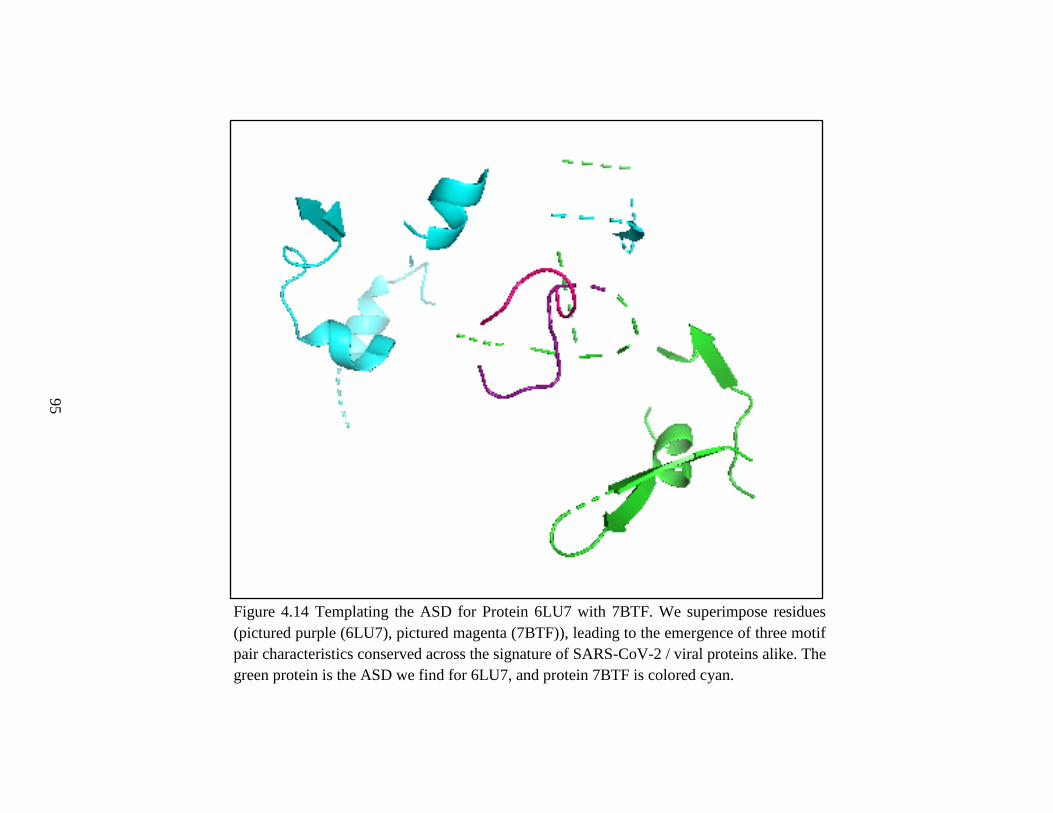
95

Figure 4.14 Templating the ASD for Protein 6LU7 with 7BTF. We superimpose residues

(pictured purple (6LU7), pictured magenta (7BTF)), leading to the emergence of three motif

pair characteristics conserved across the signature of SARS-CoV-2 / viral proteins alike. The

green protein is the ASD we find for 6LU7, and protein 7BTF is colored cyan.

96

Figure 4.15 Templating the ASD for Protein 6LU7 with 7BTF. Orientation based

on main secondary structures of the motifs conserved across the signature of

SARS-CoV-2 / viral proteins alike. The green-colored protein is 6LU7, and

pictured in cyan is 7BTF.

97

CHAPTER 5

DISCUSSION

The msTALI tool is expandable to applications for active-site identification. We

have developed a methodology highly implementable for what we have categorized as

the ASD for a protein. Further, this ties to the collective ASD for groups of proteins

exhibiting the same function. The distinguishable difference here is that our ASD

includes protein residues that are both exemplary of active-sites and supporting residues

for aiding said function. This also includes structural mechanisms conducive to active-

site exposure. Multiple proteins support these descriptions simultaneously and, with such,

incorporation of homologous characteristics become applicable to various enzymatic

activity. The classification of targeted proteins secures that conserved residues are

relevant. We also applied PDB, CATH, and other available resources to uphold findings.

Again, our methodical development is predicated on the underlying hypothesis

that the structure-sequence alignment of multiple proteins with a common function will

reveal the conserved regions (structural and sequence) containing the active-site and

motifs salient functionality. Our approach is applied to over ten classes of enzymatic

activity to support our primary aim. The successful use of msTALI focused on AMP,

ATP, FAD, FMN, Glucose, Heme, Hydrolase, NAD, Phosphate, and Steroid functioning

proteins. Evaluation of our methodology reports an average precision of 46.0% and recall

of 90.1%. Though improvements are desired, we fare upwards of 10% in comparison to

98

accepted methods. Additionally, to thwart the inconsistency faced for computational

evaluations, we have visually reported our findings too. Notably, our methodical

development's success lends to our subsequent aim to expand our tool and apply our

methodology to the current applications.

Beyond our focused study, we have employed our approach in observance of

COVID-19 studies. Here, the recourse leveraged homologous information from SARS-

CoV studies to the current SARS-CoV-2 studies and exemplified a templating approach

specifically for the ASD of COVID-19. Using structure 6LU7, we obtain an ASD with an

evaluation score of 61.91 and 96.63 percent for precision and recall. We used a

combination of the same functioning proteins with available documentation to verify our

findings. Mainly protein 7BTF was used as a primary reference structure along with

protein NSP1. We used both PDB and PDBsum for confirmed annotation. Our finding

and motif characteristics lend to regions that regulate the active-site exposure for 6LU7.

Here the practical use yields a functional shutoff framework to address COVID-19. We

mention a lid obstruction example since several SARS-CoV-2 proteins are also

categorized as hydrolases. Most notable, all the results we find are cost-effective. Our

approach requires far fewer resources than conventional research aiming to address

COVID-19 annotation, curing, and monitoring.

We assert that our methodology is suitable for a multitude of functional

descriptions. Our study on 6LU7 is the latest. Future works can always expand the

functional class annotation. However, two riveting advancements and applications to our

method are function prediction or multi-functional ASD. Function prediction is valuable

for drug-design, and, commonly, an individual protein has several roles. It would be

99

interesting to explore how these concepts impact ASD. They are beneficial for common

core understanding and advancement in our development.

100

REFERENCES

[1] W.-K. Sung, Algorithms In Bioinformatics: A Practical Introduction. Chapman &

Hall/ CRC Taylor & Francis Group, 2010.

[2] M. Hendlich, F. Rippmann, and G. Barnickel, “LIGSITE: automatic and efficient

detection of potential small molecule-binding sites in proteins,” J. Mol. Graph.

Model., vol. 15, no. 6, pp. 359–363, Dec. 1997.

[3] D. G. Levitt and L. J. Banaszak, “POCKET: A computer graphies method for

identifying and displaying protein cavities and their surrounding amino acids,” J.

Mol. Graph., vol. 10, no. 4, pp. 229–234, Dec. 1992.

[4] J. Liang, H. Edelsbrunner, and C. Woodward, “Anatomy of protein pockets and

cavities: measurement of binding site geometry and implications for ligand

design.,” Protein Sci., vol. 7, pp. 1884–1897, 1998.

[5] B. Huang and M. Schroeder, “LIGSITEcsc: predicting ligand binding sites using

the Connolly surface and degree of conservation.,” BMC Struct. Biol., vol. 6, p. 19,

2006.

[6] R. A. Laskowski, “SURFNET: A program for visualizing molecular surfaces,

cavities, and intermolecular interactions,” J. Mol. Graph., vol. 13, no. 5, pp. 323–

330, Oct. 1995.

[7] T. Singh, D. Biswas, and B. Jayaram, “AADS - An automated active site

identification, docking, and scoring protocol for protein targets based on

physicochemical descriptors,” J. Chem. Inf. Model., 2011.

[8] P. Bertolazzi, C. Guerra, and G. Liuzzi, “A global optimization algorithm for

protein surface alignment.,” BMC Bioinformatics, vol. 11, p. 488, Jan. 2010.

[9] J. S. Fetrow, A. Godzik, and J. Skolnick, “Functional Analysis of the Escherichia

coli Genome Using the Sequence-to-Structure-to-Function Paradigm :

Identification of Proteins Exhibiting the Glutaredoxin / Thioredoxin Disulfide

Oxidoreductase Activity,” J. Mol. Biol., pp. 703–711, 1998.

[10] J. Skolnick and J. S. Fetrow, “From genes to protein structure and function : novel

applications of computational approaches in the genomic era,” TIBTECH, vol. 18,

no. January, pp. 34–39, 2000.

[11] A. Gutteridge, G. J. Bartlett, and J. M. Thornton, “Using A Neural Network and

Spatial Clustering to Predict the Location of Active Sites in Enzymes,” J. Mol.

Biol., vol. 330, no. 4, pp. 719–734, Jul. 2003.

[12] A. Shulman-peleg, M. Shatsky, R. Nussinov, and H. J. Wolfson, “MultiBind and

MAPPIS : webservers for multiple alignment of protein 3D-binding sites and their

interactions,” Nucleic Acids Res., vol. 36, no. May, pp. 260–264, 2008.

[13] M. Jambon, O. Andrieu, C. Combet, G. Dele, C. Geourjon, and M. Sa, “Structural

bioinformatics The SuMo server : 3D search for protein functional sites,” vol. 21,

no. 20, pp. 3929–3930, 2005.

101

[14] M. Punta et al., “The Pfam protein families database.,” Nucleic Acids Res., vol. 40,

no. Database issue, pp. D290-301, Jan. 2012.

[15] S. Angaran, M. E. Bock, C. Garutti, and C. Guerra, “MolLoc: A web tool for the

local structural alignment of molecular surfaces,” Nucleic Acids Res., vol. 37, no.

SUPPL. 2, pp. 565–570, 2009.

[16] A. Shulman-Peleg, R. Nussinov, and H. J. Wolfson, “Recognition of functional

sites in protein structures,” J. Mol. Biol., 2004.

[17] G. Ausiello, A. Zanzoni, D. Peluso, A. Via, and M. Helmer-Citterich, “pdbFun:

Mass selection and fast comparison of annotated PDB residues,” Nucleic Acids

Res., 2005.

[18] F. Guo and L. Wang, “Computing the protein binding sites,” BMC Bioinformatics,

vol. 13, no. Suppl 10, p. S2, 2012.

[19] P. Shealy and H. Valafar, “Multiple structure alignment with msTALI.,” BMC

Bioinformatics, vol. 13, no. 1, p. 105, Jan. 2012.

[20] A. Kahraman, R. J. Morris, R. A. Laskowski, J. M. Thornton, and J. I. Centre,

“Shape Variation in Protein Binding Pockets and their Ligands,” J. Mol. Biol., pp.

283–301, 2007.

[21] X. Miao and M. G. Bryson, “TALI : Protein Structure Alignment Using Backbone

Torsion Angles.”

[22] J. D. Thompson, D. G. Higgins, and T. J. Gibson, “CLUSTAL W: improving the

sensitivity of progressive multiple sequence alignment through sequence

weighting, position-specific gap penalties and weight matrix choice.,” Nucleic

Acids Res., vol. 22, no. 22, pp. 4673–4680, 1994.

[23] S. B. Needleman and C. D. Wunsch, “A general method applicable to the search

for similiarities in the amino acid sequence of two proteins,” J. Mol. Biol., vol. 48,

no. 3, pp. 443–453, 1970.

[24] M. D. Brice, J. R. Rodgers, and O. Kennard, “The Protein Data Bank,” Eur. J.

Biochem, vol. 324, pp. 319–324, 1977.

[25] A. L. Cuff et al., “The CATH classification revisited — architectures reviewed and

new ways to characterize structural divergence in superfamilies,” Nucleic Acids

Res., vol. 37, no. November 2008, pp. 310–314, 2009.

[26] W. Humphrey, A. Dalke, and K. Schulten, “VMD: Visual Molecular Dynamics,”

1996.

[27] R. M. Hanson, J. Prilusky, Z. Renjian, T. Nakane, and J. L. Sussman, “JSmol and

the next-generation web-based representation of 3D molecular structure as applied

to proteopedia,” Israel Journal of Chemistry. 2013.

[28] C. Mattos and D. Ringe, “Locating and Characterizing Binding Sites on Proteins,”

Nat. Biotechnol., vol. 14, no. 5, pp. 595–599, 1996.

[29] J. Zhao, Y. Cao, and L. Zhang, “Exploring the computational methods for protein-

ligand binding site prediction,” Comput. Struct. Biotechnol. J., vol. 18, pp. 417–

426, 2020.

[30] N. Pandala, C. A. Cole, D. McFarland, A. Nag, and H. Valafar, “A Preliminary

Investigation in the Molecular Basis of Host Shutoff Mechanism in SARS-CoV,”

arXiv Prepr. arXiv …, vol. 1, 2020.

102

[31] D. McFarland, C. Bullock, and H. Valafar, “Evaluating Precisicon and Recall

through the Utility of msTALI via an Active Site Study on Fold Families,” Proc. -

2019 IEEE Int. Conf. Bioinforma. Biomed. BIBM 2019, pp. 1569–1572, 2019.

[32] D. McFarland, C. Bullock, B. Mueller, and H. Valafar, “Application of msTALI in

ATPase Active Site Identification,” Proc. Int. Conf. Bioinforma. Comput. Biol.,

pp. 3–9, 2016.

[33] S. Angaran, M. E. Bock, C. Garutti, and C. Guerra, “MolLoc : a web tool for the

local structural alignment of molecular surfaces,” Nucleic Acids Res., vol. 37, no.

May, pp. 565–570, 2009.

[34] I. R. Vetter, “The Structure of the G Domain of the Ras Superfamily,” in Ras

Superfamily Small G Proteins: Biology and Mechanisms 1: General Features,

Signaling, 2014, pp. 25–50.

[35] E. G. Yarmola and M. R. Bubb, “Profilin: emerging concepts and lingering

misconceptions,” Trends Biochem. Sci., vol. 31, no. 4, pp. 197–205, Apr. 2006.

[36] O. Dym and D. Eisenberg, “Sequence-structure analysis of FAD-containing

proteins,” Protein Sci., vol. 10, p. 1712, 2001.

[37] D. K. McClish, “Analyzing a Portion of the ROC Curve,” Med. Decis. Mak., vol.

9, no. 3, pp. 190–195, 1989.

[38] K. Suto et al., “How do the X-ray structure and the NMR structure of FMN-

binding protein differ?,” Acta Crystallogr. Sect. D Biol. Crystallogr., vol. 56, no.

3, pp. 368–371, 2000.

[39] R. Lu et al., “Genomic characterisation and epidemiology of 2019 novel

coronavirus: implications for virus origins and receptor binding,” Lancet, vol. 395,

no. 10224, pp. 565–574, 2020.

[40] J. Lan et al., “Structure of the SARS-CoV-2 spike receptor-binding domain bound

to the ACE2 receptor,” Nature, vol. 581, no. 7807, pp. 215–220, 2020.

[41] Y. Zhang, “I-TASSER server for protein 3D structure prediction,” BMC

Bioinformatics, vol. 9, pp. 1–8, 2008.

[42] C. Cole, C. Ott, D. Valdes, and H. Valafar, “PDBMine: A reformulation of the

protein data bank to facilitate structural data mining,” Proc. - 6th Annu. Conf.

Comput. Sci. Comput. Intell. CSCI 2019, pp. 1458–1463, 2019.

[43] M. M. C. Lai, “SARS virus: The beginning of the unraveling of a new

coronavirus,” J. Biomed. Sci., vol. 10, no. 6 II, pp. 664–675, 2003.

[44] R. A. Laskowski, J. Jabłońska, L. Pravda, R. S. Vařeková, and J. M. Thornton,

“PDBsum: Structural summaries of PDB entries,” Protein Sci., vol. 27, no. 1, pp.

129–134, 2018.

[45] Z. Jin et al., “Structure of Mpro from SARS-CoV-2 and discovery of its

inhibitors,” Nature, vol. 582, no. 7811, pp. 289–293, 2020.

[46] F. I. Khan, D. Lan, R. Durrani, W. Huan, Z. Zhao, and Y. Wang, “The lid domain

in lipases: Structural and functional determinant of enzymatic properties,” Front.

Bioeng. Biotechnol., vol. 5, no. MAR, pp. 1–13, 2017.

Documents

The Utility of Multiple Structure Torsion Angle Alignment