The User’s Guide to

MCRC software

2 | P a g e

3 | P a g e

a Chemometrics Lab., Department of Chemistry, Sharif University of Technology, Tehran, Iran

b Department of Computer Engineering, Sharif University of Technology, Tehran, Iran

Developed by:

Mehdi Jalali-Heravi* a

Hadi Parastara

Mohsen Kamalzadehb

The User’s Guide to MCRC software

4 | P a g e

Prof. R. Tauler from Department of Environmental Chemistry, IIQAB-CSIC, Barcelona, Spain

and

Dr. J. Jaumot from Department of Analytical Chemistry, University of Barcelona, Barcelona, Spain

are acknowledged for developing MCR-ALS toolbox used in this software and their valuable comments on the present software, its manual and corresponding manuscript.

The User’s Guide to MCRC software

5 | P a g e

6 | P a g e

MCRC software version 1.0

© Copyright 2010, Chemometrics Lab., Department of Chemistry, Sharif University of Technology, Tehran, Iran.

This software belongs to the holder of copyrights and it is made public on the following constraints:

It must not be changed or modified and code cannot be added. Furthermore, its codes cannot be made part of any software. In case of doubt, contact to the holder of copyrights. Mehdi Jalali-Heravi

Department of Chemistry,

Sharif University of Technology,

Tehran, Iran

Tel.: +98- 21- 66165315

Fax: +98-21- 66012983

E-mail: jalali@sharif.edu

The User’s Guide to MCRC software

7 | P a g e

8 | P a g e

Table of contents

Table of contents …………………………………….……………. 8 Preface …………………………………………………………….. 11

Introduction ……………………………………………………….. 13

About this software …………………………………………………… 14 About this manual…………………………………………………….. 15 System requirements………………………………………………….. 16 Installing MCRC software……………………………………………. 17

Data types…………………………………….……………………. 23

Importing, Exporting and Visualizing the Data………….………... 24

Data Preprocessing…………….…………………….…………….. 26

Background correction…………………………………….………….. 27 Denoising……………………………………………………………… 30 Smoothing …………………………………………………………….. 32

Chemical Rank Determination ……………….………………….... 36

Principal component analysis (PCA) ………………………………… 38 Morphological score …………………………………………………. 41 Subspace comparison (SC) …………………………………………… 44 Malinowski test ……………………………………………………….. 47 Logarithm of eigenvalues and eigenvalues ratio ……………………... 49

9 | P a g e

Local Rank Analysis …………………….………………….……… 50

Evolving factor analysis (EFA)…………………………………………….. 51 Fixed size moving window-evolving factor analysis (FSMW-EFA) …... 52 Evolving latent projective graphs (ELPGs)……………………………. 55

Resolution Methods …………………….………………………….. 57

Generation of initial estimates………………………………………… 60 Multivariate curve resolution-alternating least square (MCR-ALS)….. 64 Heuristic evolving latent projection (HELP)………………………….. 71

Peak Integration …………………………….……………………… 76

Reference…………………………………………………………………… 79

Final remarks……………………….…………………………..…… 82

10 | P a g e

11 | P a g e

Preface

Implementation of multivariate curve resolution algorithms and methods in public domain

and commercial software remain scarce, reflecting the intrinsic difficulties of developing

robust and user-friendly methods for MCR. Solving MCR problems still typically requires

user interaction and knowledge of the problem under study. In recent years great efforts have

been made by different chemometric groups for developing software (commercial or free) for

implementation of different MCR methods for analyzing multi-component systems. MCRC

software is dedicated to chemometric analysis of two-way chromatographic data such as GC-

MS and HPLC-DAD. This software offers a user-friendly tool can allow for an easy way to

perform different algorithms for prepossessing, chemical rank determination, local rank

analysis, multivariate resolution and peak integration for the analysis of multi-component

chromatographic data sets. Although MCRC software was developed for chemometric

analysis of chromatographic data, however, it may also be used for other types of multivariate

data.

This manual is designed to introduce users of MCRC software version 1.0 to the basic

operation of the program and its use in analyzing chromatographic data. It provides a

comprehensive overview of the system, including installation, data management, creating

chemometric analyses, and copying results. Since the manual is intended to get users up to

speed quickly, it concentrates on the most important features of the program, rather than

trying to cover every small detail.

NOTE: a copy of this manual in PDF format is included with the program and may be

accessed from the Help menu. In the PDF document, all of the graphs are in color.

July, 2010

12 | P a g e

13 | P a g e

1. Introduction Chromatographic analytical systems are increasingly being used for analysis of

complex samples, such as foods and essential oils. Hyphenated separation techniques

of gas chromatography-mass spectrometry (GC-MS) and high performance liquid

chromatography-diode array detection (HPLC-DAD) are intensively used for

obtaining detailed qualitative and quantitative information. However, in the case of

complex samples, the traditional approaches for handling data have many problems.

Many approaches have been proposed for situations where the eluting peaks are

completely resolved. However, analysis of chromatographic data is sometimes

hampered by different problems, mainly derived from the chromatographic separation

and/or multivariate spectroscopic measurements. For example, sometimes for

complex samples and/or the need for faster chromatographic runs, perfect separation

cannot be achieved. Also, problems with baseline drift, spectral background, presence

of different types of noise and low signal-to-noise (S/N) ratio of peaks may affect the

quality of the analysis [1-3]. Standard tools for data-analysis are insufficient for

extracting all the relevant information from the complex samples analyzed by the

chromatography. A more versatile methodology is needed for solving these

fundamental problems. Several chemometric techniques are proposed to overcome the

undesirable phenomena introduced during the chromatographic run [4-11]. Therefore,

development of software for comprehensive analysis of two-way chromatographic

data may seem necessary.

In the present manual, an integrated chemometric software is presented to apply

several different mathematical algorithms in an easy-to-use environment for solving

some chromatographic problems.

14 | P a g e

About this software MCRC software is a collection of essential and advanced chemometric routines that

work in an easy-to-use environment for solving some chromatographic problems.

MCRC software gets its name from the Multivariate Curve Resolution of two-way

Chromatographic data software. MCRC software is designed for chemists who are

not experts in programming or in advanced statistics and seek user-friendly tools for

solving chromatographic problems such as baseline drift, spectral background,

presence of different types of noise and co-elution. MCRC software consists of five groups of techniques for preprocessing, chemical

rank determination, local rank analysis, multivariate resolution and peak integration.

This software enables the analysis of complex multi-component chromatographic

signals, GC-MS and HPLC-DAD. The features of the presented software include: (a)

providing a number of preprocessing techniques, (b) implementation of different

techniques for chemical rank determination, (c) usage of iterative and non-iterative

techniques for the resolution of chromatographic data and (d) a user-friendly

graphical user interface (GUI) with variety of graphical outputs.

Running the software does not require a serious experience; however, a basic

knowledge of the underlying methods is helpful to successfully interpret the results.

15 | P a g e

About this manual

MCRC software version 1.0 includes a brief description of the theory and how to

implement the chemometric methods. The manual covers congruence analysis and

least-square fitting [12], morphological score [13], Savitzky-Golay filter [14],

principal component analysis (PCA) [15], simplified Borgen method (SBM) [16],

orthogonal projection approach (OPA) [17], subspace comparison (SC) [18], simple-

to-use interactive self-modeling mixture analysis (SIMPLISMA) [19], Malinowski’s

reduced error (RE) [20, 21], reduced eigenvalues (REV) [20, 21] and factor indicator

function (IND) [20, 21], fixed-size moving window-evolving factor analysis (FSMW-

EFA) [22], evolving latent projective graphs (ELPGs) [12], evolving factor analysis

(EFA) [23], multivariate curve resolution-alternating least square (MCR-ALS) [24-

27], heuristic evolving latent projection (HELP) [12, 28] and overall volume

integration (OVI) [29].

Only brief descriptions of the used algorithms are given here. For more information

about the methods the user is encouraged to consult the references.

16 | P a g e

System requirements

This software requires a Windows PC with Microsoft .NET Framework 2. Also,

MATLAB Component Runtime (MCR) version 7.9 is needed. MCR and Microsoft

.NET Framework 2 can be provided with the application. There are two ways for

importing data into the software; ‘New’ and ‘Open’. If you are interested to use the

‘Open’ way, make sure that Microsoft Office Interop Assemblies are installed on your

PC. The installation files for Office 2003 and 2007 are around 4 and 6 megabytes and

can be provided with the software. However, we recommend using the ‘New’ method

in case of any problems with ‘Open’.

The setup file will automatically install .NET framework if cannot find it on the host

PC. The MCR should be installed by the user. After installation, a certain string has to

be added to the ‘Path variable’ in the Windows system environmental properties. This

process is explained next in this section. The string which should be added to the path

depends on the location that the MCR has been installed. For the default location the

string will be: C:\Program Files\MATLAB\MATLAB Compiler

Runtime\v79\runtime\win32. Note that for 64 bit Windows, the last folder should be

win64: C:\Program Files\MATLAB\MATLAB Compiler Runtime\v79\runtime\win64.

In the case of different installation folders, the string should be changed accordingly.

Editing the ‘Path’ variable in Windows XP requires the following steps: (a) select the

‘My Computer’ icon on your desktop, (b) right-click the icon and select ‘Properties’

(You can also go to Control Panel > System; instead of steps (a) and (b)), (c) select

the ‘Advanced’ tab and (d) click ‘Environment Variables’. You will see two lists

containing the variables. Look for the list named ‘System Variables’. Then, find the

variable named ‘PATH’ or ‘Path’. Double click on ‘Path’ and edit it. In the appearing

window, there is a textbox named ‘Variable Value’. This contains a number of

locations separated by semicolons. Add a semicolon at the end of the list (in the case

there is no one already). Copy and paste the required string after the semicolon. Click

OK on all the open windows.

17 | P a g e

Installing MCRC software

This software is developed with Microsoft C# and makes use of MATLAB functions.

These MATLAB functions are wrapped by MATLAB Builder for .Net in DLL files

which are then used in the C# program. The functions inside the DLL files are

executed by the MATLAB Component Runtime version 7.9 which is a requirement

for this application. MCRC software should be installed as standalone software.

MCRC software files are in a self-extracting archive (.exe for PC). To install MCRC

software follows these steps:

Step 1:

Make sure you have Microsoft .Net Framework version 2 or later installed on your

PC.

Step 2:

On PC, double click the ‘setup.exe’ to install MCRC Software.

Step 3:

Run the ‘MCRInstaller.exe’ file to install MATLAB Component Runtime 7.9. This

specific version of MATLAB Component Runtime is required for this application.

Step 4:

Go to the installed program folder at corresponding directory and open the ‘MCRC

software’ folder and double click the ‘MCRC Software.exe’ for running the software.

Step 5:

Go to the ‘Help’ menu at the upper menu of the main window of the software and

open the ‘User Guide’ for obtaining more information about the state of execution of

each method.

The installation procedure is shown in Figs. 1-10.

Double click on this folder

Double click on this file

Fig. 1

Fig. 2

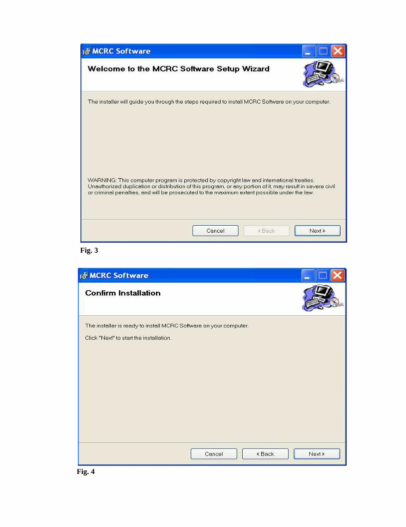
Fig. 3

Fig. 4

Fig. 5

Fig. 6

Double click on this folder

Fig. 7

Fig. 8

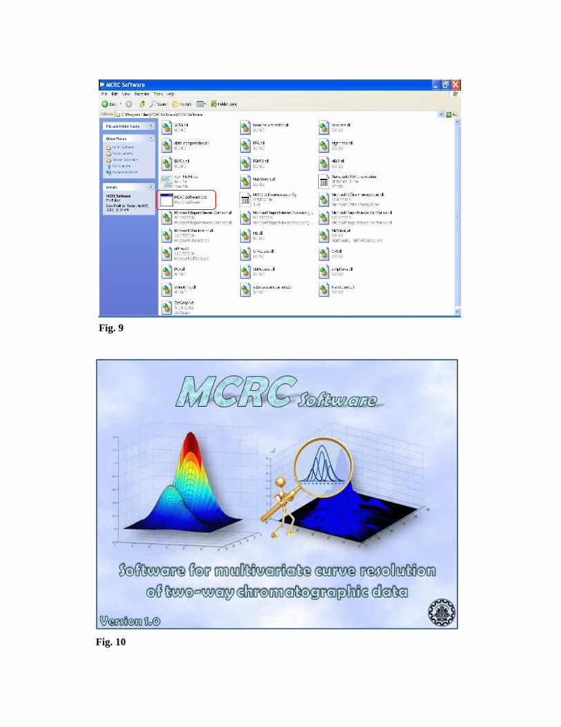
Fig. 9

Fig. 10

23 | P a g e

2. Data types

MCRC software was developed for chemometric analysis of chromatographic data;

however, it may also be used for other types of multivariate data.

This software enables the analysis of complex multi-component chromatographic

signals of gas chromatography-mass spectrometry (GC-MS) and high performance

liquid chromatography-diode array detection (HPLC-DAD). For illustrating the

versatility of the developed software and the execution of each method, a simulated

GC-MS data with three components and a given level of noise and background is

chosen. The dimension of this data is (100 × 136); 100 denote retention times as raw

variables and 136 mass-to-charges (m/z) values as column variables.

Three additional data sets are included in the software; one is simulated HPLC-DAD

data for evaluating of the potential of the software for the analysis of the HPLC-DAD

data. This data set contains three components with serious overlap. This data matrix

has 26 rows (time points) and 48 columns (wavelengths).

The second data set contains a real GC-MS peak cluster selected from the total ion

chromatogram (TIC) of the essential oil of rose flower [6]. This two-component peak

cluster has a large amount of noise and a complex pattern of elution. The dimension

of this data matrix is 41 × 231. The chemometric analysis of this peak cluster may

show the potential of MCRC software for analysis of real chromatographic data.

It is important to note that there is not limitation on the number of rows and columns.

Also, the number of rows (time points) can be more that the number of columns.

Therefore, the third data set is a four-component simulated GC-MS peak cluster. In

this data set the number of rows (retention times) is more than the number of columns

(m/z). The dimension of this data matrix is 100×20. 100 is for row variables (retention

times) and 20 is for column variables (m/z).

24 | P a g e

3. Importing, Exporting and Visualizing the Data

Usually chromatographic data acquisition software allows the user to export the

chromatographic data in ASCII (American Standard Code for Information

Interchange) format. Data files can be imported into the MCRC software in two

different modes.

The first mode is more versatile and more recommended. In this mode, the user

selects ‘File’ and then ‘New’ from the upper menu. The user can take the desired data

from somewhere else for example copy from an Excel worksheet or a MATLAB

array and paste it directly to the ‘New’ window (Right click > Paste).

In the second mode, only files with‘.xls’ format can be imported. The user selects

‘File’ and then ‘Open’ and chooses the location of the desired data.

In any case, it is very important to note that the input data must contain only the

values of intensity and other information such as the instrumental conditions,

retention times or scan numbers and wavelength or m/z values must be removed.

When two-way chromatographic data is loaded into the software, a 2D plot and the

dimensions of the input data (number of rows and columns) will appear on the right

side of the window. In addition, there is a box on the right side of the main window

of the software that the range of row variables (e.g. time points) and column variables

(e.g. wavelengths or m/z values) must be entered by user. This information can help

the user in visualizing the data and carrying on the subsequent steps of chemometric

analysis.

Fig. 11 (a) and (b) shows the main window of MCRC software before and after

importing the simulated GC-MS data. For this data, the row variables (retention

times) are in the range of 1.0 to 2.0 and column variables (m/z) from 20 to 156.

After importing the data, a larger version of the plot can be viewed by selecting

‘View’ and then ‘Plot’ from the upper menu. The plot can be saved as an image.

In addition, the input data and the obtained results after each preprocessing step can

be copied to the clipboard for future uses. This can be done by selecting ‘Data’ from

the ‘View’ menu in the menu bar.

It should be pointed out that all the techniques in the MCRC Software can be

activated by checking the check boxes below the method names.

Fig. 11 (a)

Fig. 11 (b)

4. Data preprocessing Fig. 12 shows the total ion chromatogram (TIC) of the three-component simulated

GC-MS data in the MCRC Software before applying preprocessing techniques. As it

can be seen from this figure, the input data contains a considerable amount of noise

and backgrounds contribution. Using the ‘Preprocessing’ tab the data can be

pretreated using different algorithms for the background correction, denoising and

smoothing.

The preprocessing algorithms implemented in the MCRC software improve the

capabilities of the subsequent steps.

Fig. 12

27 | P a g e

Baseline correction

Baseline correction using congruence analysis and least square fitting [12] is a very

powerful technique for removing the baseline drift and spectral background in the

chromatographic data.

For convenience, raw two-way chromatographic data in general can be divided into

two parts: one originating from the chemical constituents in the analyzed mixture,

and the other due to instrumental artifacts, called spectral background and

chromatographic baseline shift here in order to distinguish them from the ‘‘random’’

noise. Thus, raw two-way data may also be expressed as:

X = Xc + Xb or Xij = Xc,ij + Xb,ij (i = 1,…, n; j = 1,…, m) (1)

where the subscripts c and b denote constituents and background, respectively. Since

the most general systematic background for ‘‘hyphenated instrument’’ spectro-

chromatographic data is a drifting baseline in combination with a spectral

background that is approximately constant during the chromatographic run. Such a

background of two-way data could be expressed as:

Xb = t1T + 1sT or Xb,ij = ti + si (2)

Here we use vector t for the baseline shift from chromatography and sT for the

spectral absorbance vector. The vectors 1T and 1 contain only 1s and the dimensions

of the two vectors are the number of detector channels m (in wavelength or m/z in

spectra) and number of retention time n, respectively.

The chromatogram or the latent-projective graphs (ELPGs) [12] may reveal a

drifting base-line offset. Local analysis of the zero-component regions before elution

of the first chemical component starts and after the last chemical component has

eluted can together provide sufficient information for correcting a drifting base line.

The procedure for confirming and correcting a systematically drifting baseline and

spectral background using congruence analysis and least square fitting goes in five

steps:

28 | P a g e

(1) Calculate the first normalized loading vector p1,b for the zero-component region

before elution of the first chemical component starts and the first normalized

loading vector pla for the zero-component region after elution of the last

chemical component is finished.

(2) Compare the two loading vectors by means of their congruence coefficient, i.e.

calculate the scalar product Φb,a = pl,b'p l,a.

(3) If Φb,a is close to 1.0 then pl,a = p1,b meaning that the base-line offset can be

explained by the same factor (loading vector) during the whole chromatographic

elution process. In this case, the "offset" vectors tb and ta, are calculated for the

two zero-components regions.

(4) Use the simple univariate least-squares procedure to fit a straight line through all

the elements of the "offset" vectors tb and ta, with retention time as

"independent" variable. t i = b0 + b1i � � �, � � �. This procedure provides

estimates of te, for the baseline factor in the whole region between the two zero-

component regions.

(5) Collect tb, ta, and te, in one vector t and subtract tlT + lpl,bT from the data matrix

X to obtain a corrected chromatographic/spectroscopic data matrix.

This procedure provides a simple way to deal with the spectral and chromatographic

baseline offset in two-way data from hyphenated instruments. With the help of this

procedure, the spectral and chromatographic baseline offset in the two-way data can

be removed with introducing additional artifacts.

Execution of baseline correction in the MCRC software is straightforward. By

entering the points (retention times or scan numbers) in zero component regions

(ZCR), before and after the elution of the desired peak cluster and press the ‘Apply’

button, the baseline can be corrected. The plots of data before and after baseline

correction will be shown after applying this method on data. Fig. 13 (a) shows the

‘Preprocessing’ tab window and Fig. 13 (b) demonstrates the corresponding plots for

simulated GC-MS data.

Fig. 13 (a)

Fig. 13 (b)

30 | P a g e

Denoising

In the denoising step, homoscedastic noise can be reduced. This step can only be

applied to GC-MS data which contain discontinuous spectroscopic dimension. The

method of morphological score [13] is used for this purpose. This method is able to

discriminate the signal from the noise. Therefore, it can be used for removing

homoscedastic noise from data and also for chemical rank determination (next

section).

The morphological score was first presented in the chemometrics literature by Shen

et al. [13]. The method is based on the fact that the ratio of the norm of a spectrum to

the norm of its first difference is higher for a profile of a component than a profile

generated only by noise. Mathematically, it is defined by:

�� � � � �� �� � �� (3)

where MS(x) is the morphological score calculated for vector x.

MO(x) is called the morphological operator, and it calculates the difference between

sequential values of the vector x. It has been shown that the score is scale invariant

and is not affected by the magnitude of the noise; it is also independent of the

baseline offset. The morphological score of the noise level is calculated using the

formula given in Eq. (4):

���� � ���������,������� (4)

where N is the number of elements in the vector, and F is the F-test value at certain

level of confidence at (N-1,N-2) degrees of freedom. By calculation of the

morphological score of noise, it is possible to remove the spectral channels that have

the morphological score below noise. Therefore, deleting the spectral channels due to

noise would be helpful in reducing the noise in the whole signal. Due to the

discontinuity of the mass spectral, this method is applicable to GC-MS data. But in

the case of HPLC-DAD, the spectral dimension is continuous and therefore, this

method cannot be applied.

To execute this method in the MCRC software, it is only necessary to apply it on the

GC-MS data. After applying this method, the plots of desired data before and after

denoising will be shown. Fig. 14 depicts the corresponding plots for simulated GC-

MS data.

Fig. 14

32 | P a g e

Smoothing

The Savitsky-Golay filter is a smoothing filter based on polynomial regression [14].

Instead of simply using the averaging technique, the Savitsky-Golay filter employs

the regression fitting capacity to improve the smoothing results because it takes

advantage of the fitting ability of polynomial regression. However, the formulation of

the Savitsky-Golay filter is quite similar to that of the averaging filter. The major

difference between the moving-window average method and the Savitsky-Golay filter

is that the latter one is essentially a weighted average method in the form of;

�� � ����� ∑ ������� ��� (5)

In this equation, !�denotes the smoothed value while !�" are the original raw data,

where i and j are the running indices. (2m+1) is the window width and wj is the

corresponding weights in the polynomial formula through polynomial regression. It

should be noted that the first two data points, x1 and x2, cannot be smoothed in the

process. After finding for example #�, the next step is to move the window to the

right by one datum to evaluate $�. Then the procedure is repeated by moving the

window successively along the equally spaced data until all the data are exhausted. It

is noteworthy that the window width and the order of polynomial are the important

parameters in deducing the correct weights. Therefore, these parameters should be

optimized in Savitzky-Golay filter. These parameters can be changed according to the

intensity of the signal and the amount of noise.

For smoothing the import data using Savitsky-Golay filter in MCRC software, there is

an option. The user can select different window width and polynomial order and using

‘Preview’ button can see the data before and after smoothing. For example Fig. 15 (a)

and (b) demonstrates the desired plots for (width=7 and order=2) and (width=9 and

order=2).

After selecting the best window width and polynomial order by user (for example

width = 9 and order = 2), by pressing ‘Apply’ button, the initial input will be replaced

by the results of last preview and the latter will become the input for all future

functions.

Fig. 15 (a)

Fig. 15 (b)

Fig. 16 shows the ‘Preprocessing’ tab window. The small plot on the right side of the

main window is produced after applying all the preprocessing techniques. The larger

version of the plot can be viewed by selecting ‘View’ and then ‘Plot’ from the upper

menu. The plot can be saved as an image. This figure will be kept on the software

until the end of analysis. It can be seen that the background and noise are greatly

reduced.

The data after each step are available in the ‘Data’ window which was mentioned

earlier. By clicking on ‘Copy Contents’, the results will be copied to the clipboard

(Fig. 17 (a) and (b)).

Fig. 16

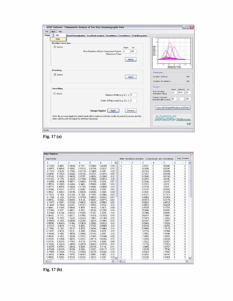
Fig. 17 (a)

Fig. 17 (b)

36 | P a g e

5. Chemical Rank Determination

The determination of the number of chemical components in a system is a crucial step

in the qualitative analysis using the data matrix. For many techniques, in an idealized

noise-free situation, this number corresponds to the matrix rank. However,

determining the chemical rank of an experimental data matrix is a difficult task

because of the following factors: (i) the presence of baseline drift and spectral

background, (ii) the presence of measurement noise and their non-assumed

distributions, (iii) heteroscedasticity of the noise, and (iv) co-linearity in the

measurement data. One can define the chemical rank as the number of relevant

chemical factors that may be extracted from the data matrix in absence of noise. Most

methods determine the chemical rank on the basis of PCA [15] or singular value

decomposition (SVD) [30]. Additionally, Malinowski proposed several criteria based

on error analysis [20, 21].

Due to the accumulation of noise in hyphenated chromatographic data such as GC-

MS and HPLC-DAD, it is often difficult to arrive at safe results by these methods

using full rank data matrix. Therefore, techniques such as subspace comparison [18]

and morphological score [13] which are based on the analysis of key spectra instead

of full rank matrices should be applied. These techniques may decrease the effect of

noise and reliable results can be obtained.

Figs. 18 (a) and (b) demonstrate the ‘Chemical Rank Determination’ tab windows

before and after entering the desired values, respectively. A brief description of

techniques used for the chemical rank determination in this software is presented here.

Fig. 18 (a)

Fig. 18 (b)

38 | P a g e

Principal Component Analysis (PCA)

As first step, PCA [15] on the input data can be performed. The input data matrix X

is subjected to the PCA bilinear decomposition. The ‘master equation’ for PCA is:

X = t1p1T + … + tppp

T + E (6)

X = TPT + E (7)

where T is the score matrix, P is the loading matrix, and they are orthogonal and

orthonormal, respectively. E is the residual matrix using p components. Also, t i and

pi are the columns of T and P, respectively. There exist a number of algorithms that

can be used for calculating PC models. These can basically be subdivided into one-

by-one component at a time algorithms (such as non-iterative partial alternating least

square (NIPALS) algorithm [30]) and all-component-at-once algorithms (such as

SVD [30]). MCRC software makes use SVD algorithm for PCA decomposition. The

SVD is:

X = USVT + E (8)

where U and V are the score and loading matrix, respectively, where U and V are

orthonormal, and S is a diagonal matrix with singular values on its diagonal. X and

E are the same as for Eq. (7). The equivalence of Eqs. (7) and (8) is given by P = V

and T = US.

The input data can be either mean centered or auto-scaled before the SVD analysis.

The maximum number of principal components can be selected by the user. The

desired plots (score, loading and eigenvalues) can be chosen by the corresponding

checkboxes. Output plots of eigenvalues, score and loadings for the simulated GC-

MS data are shown in Figs. 19 (a) – (c), respectively.

The values of score, loading and eigenvalues appear in separate windows after

applying the PCA and can be copied to the clipboard using ‘Copy Contents’ button

(Fig. 20). There is a ‘Close All Output Windows and Plots’ button on the main

window of the software. This button can be used for closing all data windows and

plots opened after applying the functions (for example windows in Fig. 20). PCA

can be used not only for obtaining a clear insight into the data but also for

determining the number of important variables in the data.

Fig. 19 (a)

Fig. 19 (b)

Fig. 19 (c)

Fig. 20

41 | P a g e

Morphological Score

Another method which is implemented in the MCRC software for the chemical rank

determination is the morphological score method [13]. As mentioned before, the

morphological score was first presented in the chemometrics literature by Shen et al.

[13]. The method is based on the fact that the ratio of the norm of a spectrum to the

norm of its first difference is higher for a profile of a component than a profile

generated only by noise. Mathematically, it is defined by:

�� � � � �� �� � �� (9)

where MS(x) is the morphological score calculated for vector x. MO(x) is called the

morphological operator, and it calculates the difference between sequential values of

the vector x. It has been shown that the score is scale invariant and is not affected by

the magnitude of the noise; it is also independent of the baseline offset. In this

method, in order to avoid accumulation of noise and obtaining reliable results, only

some key factors are analyzed instead of the full rank matrix. OPA [17] and SBM

[16] may be used as factor selection methods using this technique. Here, the level of

noise in a given confidence level or probability is calculated according to the

morphological score value. The morphological score of the noise level is calculated

using the formula given in Eq. (10):

���� � ���������,������� (10)

where N is the number of elements in the vector, and F is the F-test value at certain

level of confidence at (N-1,N-2) degrees of freedom. Then the chemical rank would

be reported by counting the number of factors with a morphological score upper than

that of the noise level (MS > MSnl). It is noteworthy that the noise level is

determined according to the amount of noise originally present in the data.

Therefore, smoothing the input data in preprocessing step is not recommended.

42 | P a g e

For the simulated GC-MS data, the user should first enter the probability level of the

calculation. For example, a probability of 0.05 which corresponds to a confidence

level of 95 % is recommended.

If SBM is selected for the factor selection the ridge parameter or offset value should

be determined. This parameter is included to prevent the presence of significant of

noise vectors in the data matrix. The offset value varies between 0 and 1.

The chosen number of factors is not critical and should only be greater than the

actual number of the components in the signal, for example it can be 8 in the case of

the simulated GC-MS data.

If OPA is selected, only the number of desired factors should be suggested by the

user (for example 8 in the case of simulated GC-MS data).

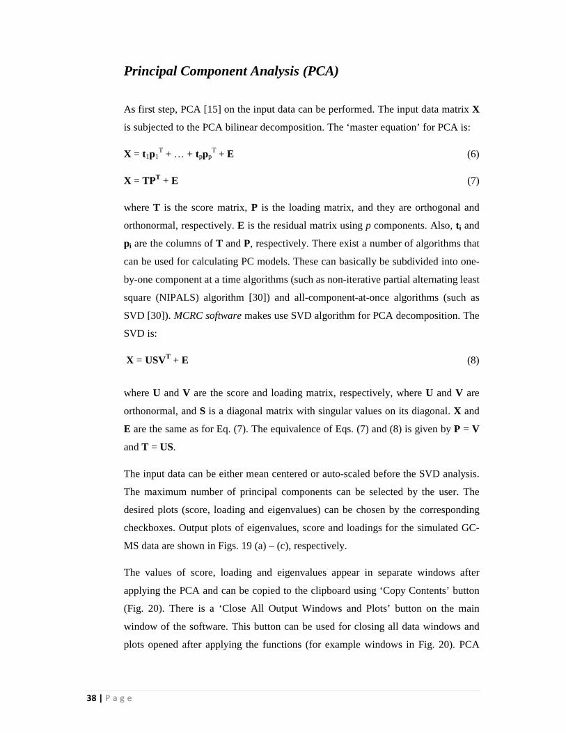
The morphological score plots using SBM and OPA are shown in Figs. 21 (a) and

(b), respectively. Although, this method is appropriate for chemical rank estimation

for GC-MS data, but it is not so suitable for HPLC-DAD data. The major reason is

due to the low level of noise in the HPLC-DAD data relative to the GC-MS data.

This can produce a wrong noise level and chemical rank for the data.

The desired data for the plots will also appear after applying the method. These data

can be copied using ‘Copy Contents’ button. Also, these windows can be closed

using ‘Close All Output Windows and Plots’ button.

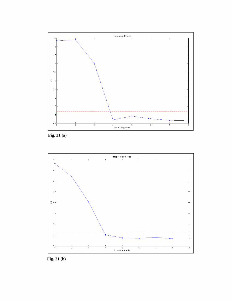
Fig. 21 (a)

Fig. 21 (b)

44 | P a g e

Subspace Comparison (SC)

Another important method for the chemical rank determination is subspace

comparison [18]. In this technique, similar to the morphological score method, key

factors are analyzed instead of the full rank data matrix.

Subspace comparison compares two subspaces, each of which is described by a set

of orthonormal vectors selected by a suitable method for factor selection such as

PCA [15], OPA [17] and SIMPLISMA [19]. Although different methods select

different key factors, if the correct number of them are selected then they will span

the same vector subspace of the full row or column space of the matrix.

Suppose two subspaces are defined as F = {f1, f2, f3, . . .,fk} and G= {g1, g2, g3, . . .,

gk}, which are taken as columns of the n×k dimensional matrices F and G. Note k

must be the same for both matrices. In this method, the vectors of F and G

orthogonalized and then the two parameters of subspace discrepancy function, D (k),

and the principal angle between subspaces, Sin2 (θK), calculate for each variable.

D (k) = k – tr (k) (11)

tr (k) = Trace (FTGGTF) (12)

D(k) is a measure of that part of the subspace which is in orthogonal complement of

the other. This function becomes zero when two subspaces are identical.

Sin2 (θK) = 1 – sK2 (13)

In this equation, sK is the eigenvalue and Sin2 (θK) is the largest principal angle as a

measure of disagreement between the subspaces.

The number of components or key factors (chemical rank) is selected from the

largest value of K when D (K) and Sin2 (θK) are equal to each other and they are

close to zero.

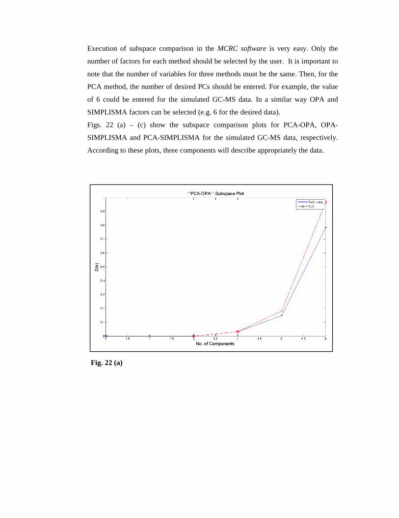
Execution of subspace comparison in the MCRC software is very easy. Only the

number of factors for each method should be selected by the user. It is important to

note that the number of variables for three methods must be the same. Then, for the

PCA method, the number of desired PCs should be entered. For example, the value

of 6 could be entered for the simulated GC-MS data. In a similar way OPA and

SIMPLISMA factors can be selected (e.g. 6 for the desired data).

Figs. 22 (a) – (c) show the subspace comparison plots for PCA-OPA, OPA-

SIMPLISMA and PCA-SIMPLISMA for the simulated GC-MS data, respectively.

According to these plots, three components will describe appropriately the data.

Fig. 22 (a)

Fig. 22 (b)

Fig. 22 (c)

47 | P a g e

Malinowski Test

The Malinowski’s reduced error (RE) and reduced error eigenvalues (REV) and

factor indicator function (IND) [20, 21] can also be used for determining the number

of significant components in the data matrix. Malinowski’s RE function can be

defined as follow:

%& � ' ∑ (���)*+���*���*�,�/� (14)

where λi is the eigenvalues, n and m are the number of rows and columns in X

matrix, respectively, and k is the number of true factors.

Malinowski’s REVs are normalized eigenvalues. An REV is defined as the

eigenvalues divided by the degree of freedom employed in its extraction and can be

defined as follow:

%&.� � (������������� (15)

Another function for determining the number of significant components is

Malinowski’s IND. This empirical function is shown in Eq. (16).

/�0 � %&��*�� (16)

where RE and k were defined previously, and l is the least of n and m.

In these methods, RE, REV and IND are plotted as a function of the number of

components in a data set. Usually one can observe a large decrease in RE and REV

as significant factors are added to the PC model. Once all of the statistically

significant variance is modeled, RE and REV level off to nearly a constant value and

thereafter slightly decreases. Additional PCs model the purely random error.

Including these factors in the PC model reduces slightly the estimated error.

Malinowski and others [20, 21] have observed that the IND function reaches a

minimum value when the correct number of factors is used in a principal component

model. Fig. 23 demonstrates the RE, REV and IND plots for the simulated GC-MS

data. In addition, the logarithmic plots are also plotted.

One can see a substantial decrease in RE and REV by going from one to two PCs.

Also, going from PC2 to PC3 shows a decrease in these functions. This decrease is

appropriately can be seen in the logarithmic curves. This strongly indicates that the

first three components are important.

Fig. 23

Logarithm of Eigenvalues & Eigenvalues Ratio

The logarithms of eigenvalues (LEV), eigenvalues ratio (EVR) and logarithms of

eigenvalues ratio (LEVR) [20] have also been reported as useful methods for

differentiating the significant components from the remaining ones. In this case, the

LEV, EVR and LEVR would be plotted against the number of components, and the

rank is determined by finding a break in the plot for the LEV plot and locating a

separate group of data points in the EVR and LEVR methods. Fig. 24 shows the

plots for the sample GC-MS data. All plots show the presence of three components

in the preprocessed data matrix.

Fig. 24

6. Local Rank Analysis

The techniques of local rank analysis give important information about the data

system under study and its structure. Different regions including zero-component,

selective and overlapped regions in chromatograms can be determined by these

methods. Evolving factor analysis (EFA) [23], fixed size moving window-evolving

factor analysis (FSMW-EFA) [22] and evolving latent projective graphs (ELPGs)

[12] techniques are applied for this purpose. EFA, FSMW-EFA and all their derived

approaches are called local rank analysis methods because they look at the

chromatograms in a local fashion, with repeated analyses of restricted elution

windows of the data set. Other exploratory tools look at the complete

chromatographic data with the aim of locating the most representative elution times,

i.e. the purest spectra, or the most representative detector channels, i.e. the purest

elution profiles, in the chromatographic run.

Here a brief description of each method and the state of execution in the MCRC

software is presented. Fig. 25 shows the ‘Local Rank Analysis’ tab window. In this

window three methods of EFA, FSMW-EFA and ELPGs are included.

Fig. 25

51 | P a g e

Evolving Factor Analysis (EFA)

Evolving factor analysis (EFA) was the parent method conceived by Maeder et al.

[12] to study sequential evolving processes, such as chemical reactions or elution in

chromatography. Mimicking a chromatographic analysis, where the chromatogram

is formed recording successive spectra as a function of time, EFA performs PCA

analyses on gradually expanding data matrices in the elution direction, enlarged by

adding a new spectrum (detector response) at a time. This procedure is performed

from top to bottom of the data set (forward EFA) and from bottom to top (backward

EFA) to investigate the emergence and the decay of the eluting compounds,

respectively.

Fig. 26 shows the EFA results for a three-component GC-MS data table. The

overlaid forward EFA plot and backward EFA plot are built by representing the

log(eigenvalues) of each PCA analysis vs. the elution time related to the last row

included in the window analyzed. The lines connecting all the analogous eigenvalues

(ev), i.e., all the 1st ev., the 2nd ev., the ith ev.,. . . indicate the evolution of the

magnitude of eigenvalues along the elution process and, as a consequence, the

variation linked to the eluting compounds. A new eigenvalue line seen above the

noise level, marked by the pool of non-significant eigenvalues, indicates the

emergence (forward EFA) or decay (backward EFA) of an eluting compound.

Considering the simplest case, where components are eluting sequentially and there

are no embedded peaks (i.e., peaks eluting completely under a major one), the time

range between the point where the first forward EFA line and the last backward EFA

line arise from noise defines the elution window (time range of compound elution)

for the first eluting compound. The time range out of the elution windows the

complementary zero concentration window (time range where a compound is

absent). This procedure can be performed analogously for all eluting compounds in

the data set [31]. The knowledge of these windows is essential for many resolution

methods.

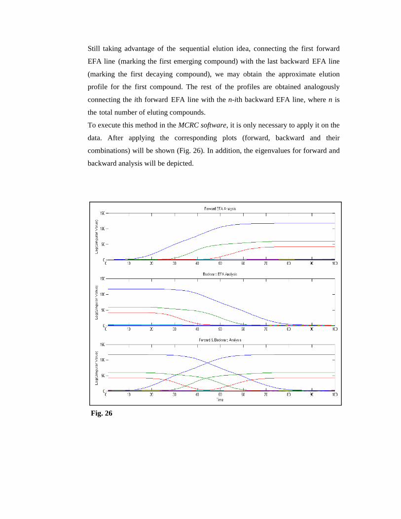
Still taking advantage of the sequential elution idea, connecting the first forward

EFA line (marking the first emerging compound) with the last backward EFA line

(marking the first decaying compound), we may obtain the approximate elution

profile for the first compound. The rest of the profiles are obtained analogously

connecting the ith forward EFA line with the n-ith backward EFA line, where n is

the total number of eluting compounds. To execute this method in the MCRC software, it is only necessary to apply it on the

data. After applying the corresponding plots (forward, backward and their

combinations) will be shown (Fig. 26). In addition, the eigenvalues for forward and

backward analysis will be depicted.

Fig. 26

53 | P a g e

Fixed-Size Moving Window-EFA (FSMW-EFA)

Another family of methods derived from EFA performs PCA analyses on windows

of fixed size that are moved along the dataset. The most widely used approach of

this kind is fixed size moving window-evolving factor analysis (FSMW-EFA),

developed by Keller et al. [22]. In this method, PCA analyses are performed on fixed

size windows moved row by row downwards along the elution direction of the data

set. The FSMW-EFA plot shows the eigenvalues obtained in all the PCA analyses as

it was done in EFA. This representation contains the information on the compound

overlap in the elution direction. In FSMW-EFA plots, the logarithmic of eigenvalues

higher than the noise level shows the presence of a new component. For a system of

one species, only one curve is higher than the noise level in its FSMW-EFA plot. If

the local rank is two, there are two components co-eluting, and so forth. The flat area

in this plot shows the pure selective regions for one single component and the peak-

shaped region represents the overlapping region containing at least two components.

Thus, elution ranges where two eigenvalue lines arise from the noise level indicate

the presence of two overlapped compounds. In general, the number of compounds

overlapping in a certain time range equals the number of eigenvalue lines above the

noise level. FSMWEFA is particularly useful for the detection of selective elution

regions for the different compounds, i.e., zones where only one compound is

present. When such zones are present, obtaining the pure spectra of the related

compounds is straightforward. They are thus of great help to decrease the

uncertainty linked to the chromatographic resolution results. FSMW-EFA was

created as a method more capable to detect impurities or minor compounds than

EFA due to the local analysis of small elution windows. This sensitivity explained

the widespread use of this method to address peak purity problems [32, 33].

Therefore, both the number of chemical species at every scan number and patters of

elution for concentration profiles can be obtained. Also, from this plot one can

obtain some information about the zero components, overlap and selective regions,

i.e. the local rank information are obtained. In order to further confirm the

conclusion obtained from the FSMW-EFA, the use of ELPG plots is also helpful.

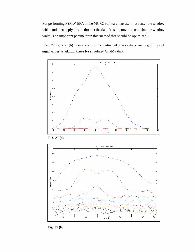
For performing FSMW-EFA in the MCRC software, the user must enter the window

width and then apply this method on the data. It is important to note that the window

width is an important parameter in this method that should be optimized.

Figs. 27 (a) and (b) demonstrate the variation of eigenvalues and logarithms of

eigenvalues vs. elution times for simulated GC-MS data.

Fig. 27 (a)

Fig. 27 (b)

55 | P a g e

Evolving Latent Projective Graphs (ELPGs)

The ELPG [12] plot is actually a principal component projective plot. In the ELPG

plot using the chromatographic direction, a straight-line region represents a pure

selective region for one single component, while the curving part regions denote the

overlapping regions containing at least two components.

There are at least four advantages of using the ELPGs:

1. In bivariate score plot, a straight-line segment pointing to the origin suggests

selective information in the retention time direction. As for the bivariate loading

plot, a straight-line segment pointing to the origin suggests selective information in

the spectral direction. The concept of ‘straight line’ here is, of course, in the sense of

least squares.

2. The evolving information of the appearance and disappearance of the chemical

components in the retention time direction can also be provided in ELPG. If one can

produce the three-dimensional ELPG for the peak cluster with more than three

components, the ELPG can provide more depicting insight about the data structure.

3. Information enabling the detection of shifts of the chromatographic baseline and

instrumental background is also provided in ELPG. If there is an offset in the

chromatogram, the points will not concentrate at the origin in the plot even if one

includes the zero-component regions in the data.

4. ELPG is also a very good diagnostic tool to identify the embedded peaks in the

chromatogram. This information is very important for resolving concentration

profiles. The ELPG works like a microscope to assist one to see the details of the

data structure of two-way data.

Execution of this method in the MCRC software is very straightforward. The user

can plot the 2-dimensional (2D) (Fig. 28 (a)) or 3-dimensional (3D) (Fig. 28 (b))

graphs representation of these plots using the MCRC software.

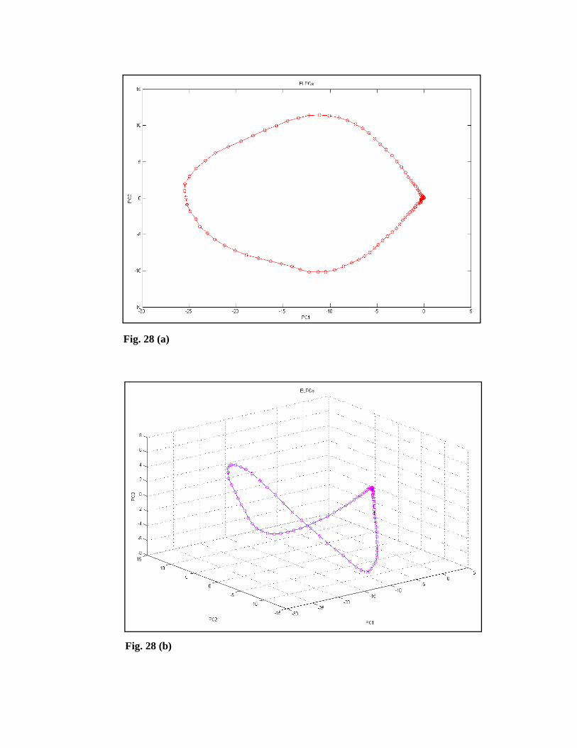
Fig. 28 (b)

Fig. 28 (a)

57 | P a g e

7. Resolution Methods

Multivariate resolution methods are factor analysis tools designed to find the real

underlying chromatographic profile and pure mass spectrum of each component

using only the recorded two-way data matrix.

A two-dimensional chromatographic data X (m×n) produced by a hyphenated

instrument can be expressed as the product of two factor matrices as follows;

Xm×n = Cm×pST

n×p + E (17)

In this equation, Xm×n denotes response matrix representing p components of m

spectra measured at regular time intervals and at n different wavelengths or m/z

values. Matrix C is composed of p columns, each describing the chromatographic

profile of a pure chemical species. Similarly, the matrix ST consists of p rows

corresponding to the pure spectra of the chemical components. Matrix E denotes the

noise of the measurement. The superscript T means the matrix is transposed. The

main goal of the multivariate curve resolution techniques is the decomposition of the

response matrix according to Eq. (17).

Multivariate curve resolution (MCR) methods have been classified in different ways

[34] including both hard-modeling (HMCR) and self-modeling curve resolution

(SMCR) methods. Hard-modeling methods force a specific mathematical model for

example the shape of elution profiles or the shape of a curve in kinetics. Self-

modeling methods do not demand a priori information about the spectral or

concentration profiles but apply natural constraints [34] such as unimodality and

non-negativity. SMCR can further be categorized as iterative and non-iterative

according to the algorithm used.

Iterative resolution methods obtain the resolved concentration and response matrices

through the one-at-a-time refinement or simultaneous refinement of the profiles in

C, in ST, or in both matrices at each cycle of the optimization process. The profiles

in C or ST are “tailored” according to the chemical properties and the mathematical

features of each particular data set. The iterative process stops when a convergence

criterion (e.g., a preset number of iterative cycles is exceeded or the lack of fit goes

below a certain value) is fulfilled.

58 | P a g e

Iterative resolution methods are in general more versatile than non-iterative

methods. They can be applied to more diverse problems, e.g., data sets with partial

or incomplete selectivity in the concentration or spectral domains, and to data sets

with concentration profiles that evolve sequentially or non-sequentially. Prior

knowledge about the data set (chemical or related to mathematical features) can be

used in the optimization process, but it is not strictly necessary.

Commonly used iterative methods include iterative target transformation factor

analysis (ITTFA) [35, 36], multivariate curve resolution-alternating least squares

(MCR-ALS) [24-27], resolving factor analysis (RFA) [37] and multivariate curve

resolution-objective function minimization (MCR-FMIN) [8, 38].

The generation of initial estimates for starting the iterative optimization process and

applying proper constraints such as non-negativity, unimodality and selectivity,

during the optimization process are important for obtaining the more unique

responses.

Most non-iterative methods are one-step calculation algorithms that focus on the

one-at-a-time recovery of either the concentration or the response profile of each

component. Once all of the concentration (C) or response (S) profiles are recovered,

the other member of the matrix pair, C and S, is obtained by least-squares (LS)

according to the general MCR model, X = CST [39, 40].

Methods which are non-iterative in nature include evolving factor analysis (EFA)

[23], window factor analysis (WFA) [41], heuristic evolving latent projections

(HELP) [12, 28], sub-window factor analysis (SFA) [42] and parallel vector analysis

(PVA) [43].

Non-iterative methods use information from local-rank maps or concentration

windows in a characteristic way. In mathematical terms, these windows define

subspaces where the different compounds are present or absent. The subspaces can

be combined in clever ways through projections or by extraction of common vectors

(profiles) to obtain the profiles sought. Non-iterative methods are fast, but they have

clear limitations in their applicability because of the difficulties associated with

correct definition of concentration windows and local rank.

In many situations, the MCR solutions are not unique. Very often, rotational and

intensity ambiguities may present in MCR solutions. It means that, instead of a

unique solution, a range of feasible solutions that fit the data equally well may be

obtained. These bands of feasible solutions can be drastically reduced when

59 | P a g e

constraints are applied during the estimation of concentration and spectral profiles.

Several procedures have been described in the literature about how to find the bands

of feasible solutions associated to MCR solutions [44-46].

The MCR-ALS and HELP are common MCR techniques and both are available in

the MCRC software. A brief description of these methods is presented below.

60 | P a g e

Generation of Initial Estimates

The iterative optimization of the profiles in C or ST starts by using a matrix or a set

of profiles with the same size as C or ST with rough approximations of the

concentration profiles or spectra that will be obtained as the final results. This matrix

contains the initial estimates to be used in the resolution process. In general, the use

of nonrandom estimates shortens the iterative optimization process and helps to

avoid convergence to a local optimum different from the desired solution. It is

sensible to use chemically meaningful estimates if we have a way to obtain them

easily or if the necessary information is available. Whether the initial estimates of C-

type or ST-type are selected depends on which type of profiles is less overlapped, on

which direction of the matrix is more information available or simply on the will of

the chemist.

There are several chemometric methods to calculate these initial estimates; some of

them are particularly suitable when the data consists of evolutionary profiles of a

process, such as EFA [12], whereas some others mathematically select the purest

rows or columns of the data matrix as initial profiles such as SIMPLISMA [19],

OPA [17] or SBM [16].

The MCRC software uses these methods for estimating the initial guess of

concentration and spectral profiles. Fig. 29 shows the Resolution 1 tab window. In

this window the Number of Components boxes for each method should be filled in.

Additionally, the value of Noise Percent in the SIMPLISMA method and Ridge

Parameter in the SBM should be entered. The Ridge parameter is included to

prevent the presence of significant of noise vectors in the data matrix. The value of

this parameter varies between 0 and 1. The user can select whether concentration or

spectral profiles are obtained. Figs. 30 (a)-(d) show the initial estimates of the

concentration profiles using the methods of EFA, SIMPLISMA, OPA, and SBM,

respectively. Also, the minimum number of components for the SBM method is

three.

Fig. 29

Fig. 30 (a)

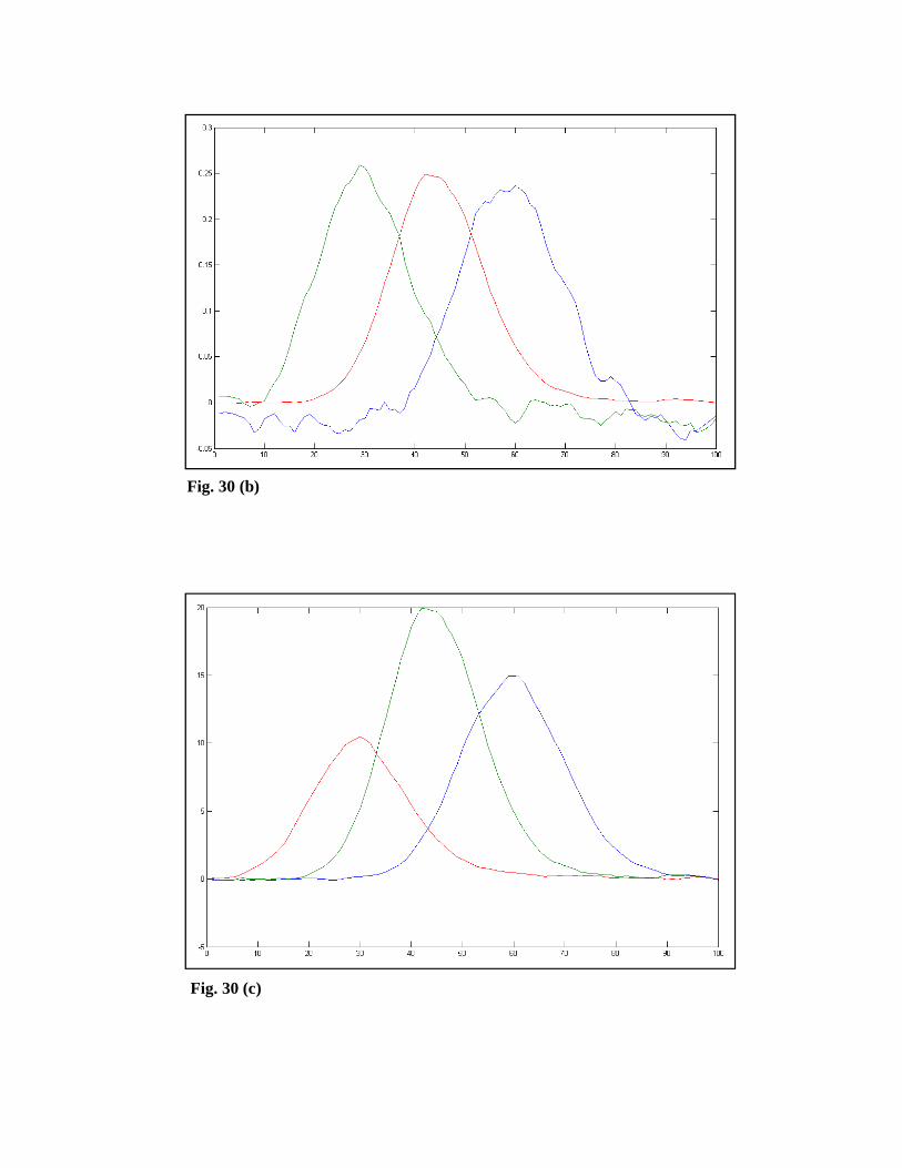
Fig. 30 (b)

Fig. 30 (c)

Fig. 30 (d)

64 | P a g e

Multivariate curve resolution-alternating least squares (MCR-ALS)

MCR-ALS is a specific implementation of ALS that has been proposed and

developed by Tauler’s group [24-27]. It is an iterative resolution method whose

algorithm is related in the most straightforward manner to the basic MCR model.

Thus, MCR-ALS finds iteratively the matrices of concentration profiles and spectra

through the optimization of C-type or ST-type estimates by a constrained alternating

least-squares procedure. In this method, neither the C nor the ST matrix has priority

over the other and the two full matrices are used in each iterative cycle. The general

operating procedure of MCR-ALS includes the following:

1. Determination of the number of compounds in X.

2. Generation of initial estimates (e.g., C-type matrix).

3. Calculation of ST under constraints.

4. Calculation of C under constraints.

5. Reproduction of X from the product of C and ST.

6. Go to step (3) until convergence is achieved.

The number of compounds in X can be determined using ‘Chemical Rank

Determination’ step or can be known beforehand. In any case, the number obtained

must not be considered a critical parameter and resolution of the system using

different numbers of components is the usual and recommended practice. The initial

estimates used should be chemically meaningful and can be generated using the

methods described in previous section that best suit the nature of the data set. The

core of the MCR-ALS method consists of solving the following two least-squares

problems under the suitable constraints:

���12 34516 7 1 8 �293 (18)

����2 34516 7 1 8 �293 (19)

In these two equations, the norm of the residuals between the PCA reproduced data,

XPCA, using the selected number of components, and the ALS reproduced data using

65 | P a g e

the least-squares estimates of C and ST matrices, 1 8 and �29, is alternatively

minimized keeping constant 1 8 (Equation (18)) or �29 (Equation (19)). The explicit

least squares solution of Equation (18) is:

�29 � 12912���1294516 (20)

Or in equivalent form:

�29 � 12� 4516 (21)

where 12� is the pseudoinverse of the concentration matrix. Likewise, the explicit

least-squares solution of Equation (19) is:

:8 � 4516;8�29�2��� (22)

or

:8 � 4516�2� (23)

where �2� is the pseudoinverse of the spectral matrix.

The two least-squares problems in Equations (18) and (19) are solved sequentially in

each iterative cycle, that is, the spectral matrix ST is calculated and then used to

obtain the concentration matrix C. Note that the matrix used to check for the

convergence of the optimization procedure is frequently not the experimental matrix,

X, but the reproduced matrix from a PCA model with a number of components equal

to the number of chemical compounds in the system, XPCA. This de-noised matrix

keeps all the relevant chemical information on the original data set and helps to

evaluate in a more reliable way the convergence of the optimized profiles toward the

solutions sought. The convergence criterion in the alternating least-squares

optimization is typically based on the comparison of the fit obtained in two

consecutive iterations. When the relative difference in fit is below a threshold value,

the optimization is finished. Other possibilities include setting a maximum number

of iterative cycles as a stop criterion or comparing the shape of the resolved

66 | P a g e

concentration profiles and spectra in consecutive iterations. Although the difference

in fit between iterations is the most commonly used criterion to stop the optimization

process, it is also recommended to monitor the evolution of the profile shapes to be

sure that the optimal solution has been obtained from all possible points of view. As

long as inappropriate constraints are not employed and the core bilinear model is

obeyed, MCR-ALS will usually result in a feasible solution, although rotational

and/or intensity ambiguities can still exist depending on the actual system under

study. During the ALS optimization, several constraints can be applied to model the

shapes of the C or ST profiles such as non-negativity, unimodality, normalization

and selectivity (local rank). In reference 27, the MCR-ALS method and graphical

user interface (GUI) developed by Jaumot et al. is explained in more detail. In the

present MCRC software, this MCR-ALS GUI is kept practically equal to the one

previously developed. Figures of merit of the optimization procedure are the

percentage of lack of fit (LOF), the percentage of explained variance (R2) and the

standard deviation of the residuals with respect to the experimental data (σ).

LOF is defined as the difference among the input data X and the data reproduced

from the CST product obtained by MCR techniques. This value is calculated

according to the expression:

<�� %� � �>> ?∑ @����,�∑ ����,� (24)

Where xij designs an element of the input data matrix X and eij is the related residual

obtained from the difference between the input element and the MCR reproduction.

R2 and σ are calculated according to following expressions where xij and eij are the

same as above and nrows and ncolumns are the number of rows and columns in the X

matrix.

%� � ∑ ���� ∑ @�,���,��,� ∑ ����,� (25)

A � � ∑ @����,��BC�D �EC�F��D (26)

67 | P a g e

The MCR-ALS optimization dialog boxes that appear during the MCR-ALS

execution are mainly related to: (a) input of initial information, (b) selection of the

constraints and selection of the optimization parameters and (c) display of the

resolution results. The first dialog box corresponds to the Selection of the data set

window. In this window the data matrix and the initial estimate boxes should be

filled in (Fig. 31 (a), input in data matrix box and one of the estimations EFA,

SIMPLISMA, OPA and SBM in initial estimate box). Once these matrices have

been selected, six different plots corresponding to the columns and rows of the input

data matrix, initial estimate profiles and score and loading plots of PCA are

obtained.

By clicking the Continue button, the software will go directly to the Selection of ALS

constraints window (Fig. 31 (b)). After loading this window in Fig. 31 (b), the only

active buttons are those to select which constraints should be applied. When one

particular constraint and the matching checkbox button are selected, new options are

gradually activated to give the details on where and how the constraints should come

into play in the resolution process.

Fig. 31 (a)

Fig. 31 (b)

When no closure constraint is selected, as for the GC-MS example, a new window

will open suggesting the use of an alternative normalization to avoid scale problems

during ALS optimization (see Fig. 31 (c)). Once the constraints are selected, the

choice of the optimization parameters and the information needed to present the

output of the resolution method are carried out in the same way for the data matrix.

By clicking the Optimize button, the optimization procedure starts showing the

partial results obtained in different iterations. When graphical output has been

selected, the MCR-ALS resolved profiles are graphically shown after each iteration.

Once convergence is achieved or after the maximum number of iterations is

exceeded or in the case of divergence, the optimal resolution results will be shown

(Fig. 31 (d)). In this window, a plot of the resolved concentration and spectral

profiles is given as well as figures of merit related to the optimization results. More

details for the state of the execution of this toolbox are given in the reference 27.

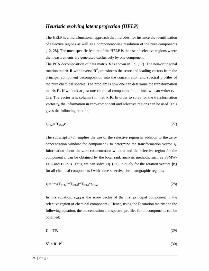
Finally, the corresponding data for exporting from the MCRC Software and

subsequent analysis can be appeared by clicking the Retrieve Results button in the

Resolution 1 tab window. Two windows containing the values of concentration and

spectral profiles will appear (Fig. 32).

Fig. 31 (c)

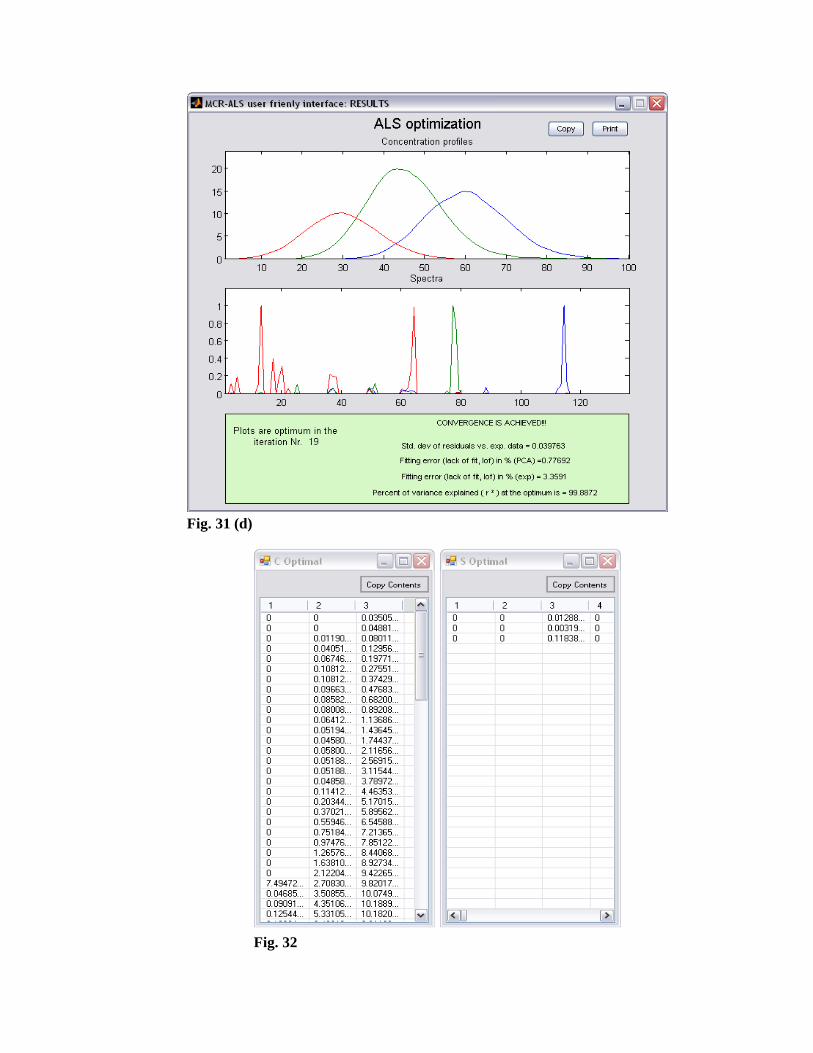
Fig. 31 (d)

Fig. 32

71 | P a g e

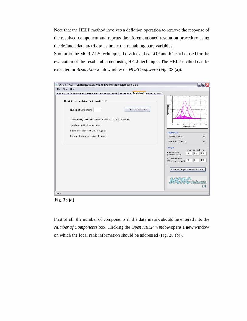
Heuristic evolving latent projection (HELP)

The HELP is a multifunctional approach that includes, for instance the identification

of selective regions as well as a component-wise resolution of the pure components

[12, 28]. The most specific feature of the HELP is the use of selective regions where

the measurements are generated exclusively by one component.

The PCA decomposition of data matrix X is shown in Eq. (17). The non-orthogonal

rotation matrix R with inverse R-1, transforms the score and loading vectors from the

principal component decomposition into the concentration and spectral profiles of

the pure chemical species. The problem is how one can determine the transformation

matrix R. If we look at just one chemical component i at a time, we can write; ci =

Tr i. The vector r i is column i in matrix R. In order to solve for the transformation

vector r i, the information in zero-component and selective regions can be used. This

gives the following relation;

cs+o,i = Ts+o,ir i (27)

The subscript s+0,i implies the use of the selective region in addition to the zero-

concentration window for component i to determine the transformation vector r i.

Information about the zero concentration window and the selective region for the

component i, can be obtained by the local rank analysis methods, such as FSMW-

EFA and ELPGs. Thus, we can solve Eq. (27) uniquely for the rotation vectors {r i}

for all chemical components i with some selective chromatographic regions;

r i = inv(Ts+0,iT*Ts+0,i)*Ts+0,i*cs+0,i (28)

In this equation, cs+0,i is the score vector of the first principal component in the

selective region of chemical component i. Hence, using the R rotation matrix and the

following equation, the concentration and spectral profiles for all components can be

obtained;

C = TR (29)

ST = R-1PT (30)

Note that the HELP method involves a deflation operation to remove the response of

the resolved component and repeats the aforementioned resolution procedure using

the deflated data matrix to estimate the remaining pure variables.

Similar to the MCR-ALS technique, the values of σ, LOF and R2 can be used for the

evaluation of the results obtained using HELP technique. The HELP method can be

executed in Resolution 2 tab window of MCRC software (Fig. 33 (a)).

First of all, the number of components in the data matrix should be entered into the

Number of Components box. Clicking the Open HELP Window opens a new window

on which the local rank information should be addressed (Fig. 26 (b)).

Fig. 33 (a)

This information can be obtained from the Local Rank Analysis step using EFA,

FSMW-EFA and ELPGs. For each component, zero-component and selective

regions should be selected. Zero-component region (ZCR) considers a retention time

range in which no compound has been eluted. In selective regions only one

component could be present. In other words, the local rank is one in this range. In

addition, each component has usually two zero-components and one selective region

except for the first and last components which have only one ZCR. Therefore, the

user can tick the check box for activating the second ZCR in the HELP window (Fig.

33 (b)). After entering the corresponding information in this window for each

component, clicking the Apply button starts the calculation of the HELP solutions.

Fig. 33 (c) shows the corresponding profiles obtained using this method and the

corresponding values is shown in Fig. 33 (d).

Fig. 26 (b)

Fig. 33 (b)

Fig. 33 (c)

Fig. 33 (d)

Finally, after calculating the HELP solutions, the statistical parameters can be

displayed in the Resolution 2 window similar to the MCR-ALS (Fig 34). These

parameters are useful in comparison with the results of the two methods (MCR-ALS

and HELP).

Fig. 34

76 | P a g e

8. Peak Integration

The method of overall volume integration (OVI) [29] is carried out for computing

the amount of each component after resolving the chromatograms and mass spectra.

The total two-way response of each component can be obtained from the outer

product of concentration and spectrum vectors. The total amount of each component

is proportional to the overall volume of its two-way response. The advantage of this

quantitative method over the general peak-area integration is that all mass spectral

intensities are taken into consideration. Also, it avoids the disadvantage that general

peak area approximately treated by peak split.

Execution of the OVI in the MCRC software is very simple. Peak Integration tab

window is shown in Figs. 35 (a) and (b). In this window the corresponding matrix

and method boxes should be filled in.

In the first box, the input data matrix (either processed or not) and the pure data

matrix for each component can be selected. In a similar way, in the second box the

desired method (MCR-ALS and/or HELP) should be selected by the user.

By clicking the Apply button, the software calculates the peak area for each data

matrix and the relative percentage for each one relative to the whole signal can be

calculated.

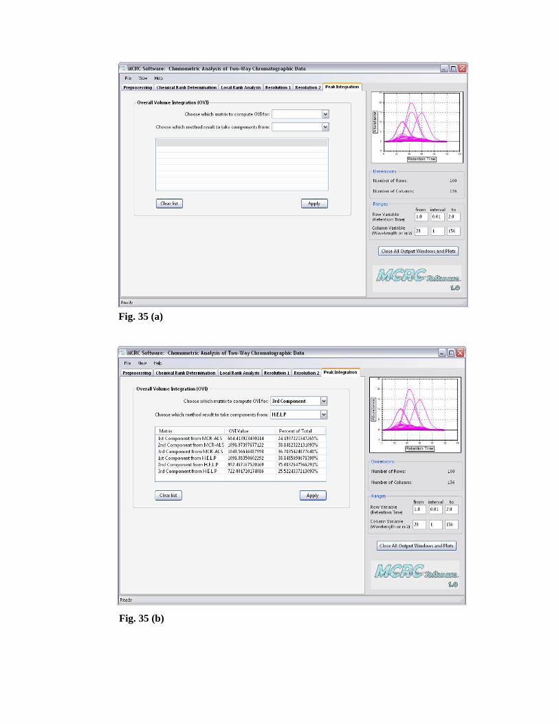
Fig. 35 (a)

Fig. 35 (b)

78 | P a g e

79 | P a g e

9. References

[1] J.M. Amigo, T. Skov, J. Coello, M. Maspoch, R. Bro, Trends Anal. Chem. 27

(2008) 714.

[2] T. Skov, R. Bro, Anal. Bioanal. Chem. 390 (2008) 281.

[3] J.M. Amigo, T. Skov, R. Bro, Chem. Rev. (2010) doi: 10.1021/cr900394n

[4] M. Katajamaa, M. Oresic, J. Chromatogr. A 1158 (2007) 318.

[5] M. Jalali-Heravi, H. Parastar, H. Sereshti, J. Chromatogr. A 1217 (2010) 4850.

[6] M. Jalali-Heravi, H. Parastar, H. Sereshti, Anal. Chim. Acta 623 (2008) 11.

[7] N.P.V. Nielsen, J.M. Carstensen, J. Smedsgaard, J. Chromatogr. A 805 (1998)

17.

[8] M. Jalali-Heravi, H. Parastar, Chemom. Intell. Lab Syst. 101 (2010) 1.

[9] G. Vivo-Truyols, J.R. Torres-Lapasio, M.C. Garcia-Alvarez-Coque, P.J.

Schoenmakers, J. Chromatogr. A 1158 (2007) 258.

[10] J.W.H. Wong, C. Durante, H.M. Cartwright, Anal. Chem. 77 (2005) 5655.

[11] M. Jalali-Heravi, H. Parastar, H. Ebrahimi-Najafabadi, Anal. Chim. Acta 662

(2010) 143.

[12] O.M. Kvalheim, Y.Z. Liang, Anal. Chem., 64 (1992) 936.

[13] H. Shen, Y.Z. Liang, O.M. Kvalheim, R. Manne, Chemom. Intell. Lab. Syst.,

51 (2000) 49.

[14] R.G. Brereton, Chemometrics: Data Analysis for the Laboratory and Chemical

Plant, Wiley, New York, 2002.

[15] S. Wold, K. Esbensen, P. Geladi, Chemom. Intell. Lab. Syst., 2 (1987) 37.

[16] B.V. Grande, R. Manne, Chemom. Intell. Lab. Syst., 50 (2000) 19.

[17] F. Cuesta Sanchez, J. Toft, B. Van den Bogaert, D.L. Massart, Anal. Chem.,

68 (1996) 79.

80 | P a g e

[18] H. Shen, L. Stordrange, R. Mane, O.V. Kvalheim, Y.Z. Liang,

Chemom. Intell. Lab. Syst., 51 (2002) 37.

[19] W. Windig, J. Guilment, Anal. Chem., 63 (1991) 1425.

[20] M. Wasim, R.G. Brereton, Chemom. Intell. Lab. Systs., 72 (2004) 133.

[21] Malinowski, E.R., Factor Analysis of Chemistry, 2nd ed., John Wiley & Sons,

New York, 1991.

[22] H.L. Keller, D.L. Massart, Anal. Chim. Acta, 246 (1991) 379.

[23] M. Maeder, Anal. Chem., 59 (1987) 527.

[24] S. Navea, A. de Juan, R. Tauler, Anal. Chim. Acta, 446 (2001) 185.

[25] A. de Juan, R. Tauler, Anal. Chim. Acta, 500 (2003) 195.

[26] R. Tauler, A. Smilde, B. Kowalski, J. Chemom., 9 (1995) 31.

[27] J. Jaumot, R. Gargallo, A. de Juan, R. Tauler, Chemom. Intell. Lab. Syst., 76

(2005) 101.

[28] Y.Z. Liang, O.M. Kvalheim, H.R. Keller, D.L. Massart, P. Kiechle, F. Erni,

Anal. Chem., 64 (1992) 946.

[29] F. Gong, Y.Z. Liang, H. Cui, F.T. Chau, B.T.P. Chan, J. Chromatogr. A, 909

(2001) 237.

[30] K.H. Esbensen, P. Geladi, in: S.D. Brown, R. Tauler, B. Walczak (Eds.),

Comprehensive Chemometrics: Chemical and Biochemical Data Analysis, vol.

2, Elsevier, Amsterdam, Netherlands, 2009, pp. 211–224.

[31] A. de Juan, R. Tauler, J. Chromatogr. A, 1158 (2007) 184.

[32] J.A. Gilliard, J.L. Cumps, B.L. Tilquin, Chemom. Intell. Lab. Syst. 21 (1993)

235.

[33] K. de Braekeleer, A. de Juan, D.L. Massart, J. Chromatogr. A 832 (1999) 67.

[34] S.C. Rutan, A. de Juan, R. Tauler, in: S.D. Brown, R. Tauler, B. Walczak

81 | P a g e

(Eds.), Comprehensive Chemometrics: Chemical and Biochemical Data

Analysis, vol. 2, Elsevier, Amsterdam, Netherlands, 2009, pp. 249–257.

[35] P.J. Gemperline, J. Chem. Inf. Comput. Sci. 24 (1984) 206.

[36] B.G.M.Vandeginste,W. Derks, G. Kateman, Anal. Chim. Acta 173 (1985) 253.

[37] C. Mason, M. Maeder, A. Whiston, Anal. Chem. 73 (2001) 1587.

[38] R. Tauler, Anal. Chim. Acta 595 (2007) 289.

[39] J.H. Jiang, Y. Ozaki, Appl. Spectrosc. Rev. 37 (2002) 321.

[40] J.H. Jiang, Y. Liang, Y. Ozaki, Chemom. Intell. Lab. Syst. 71 (2004) 1–12.

[41] E.R. Malonowski, J. Chemom. 6 (1992) 29.

[42] R. Manne, H. Shen, Y. Liang, Chemom. Intell. Lab. Syst. 45 (1999) 171.

[43] J.H. Jiang, S. Sasic, R.Q. Yu, Y. Ozaki, J. Chemom. 17 (2003) 186.

[44] P.J. Gemperline, Anal. Chem. 71 (1999) 5398.

[45] R. Tauler, J. Chemom. 15 (2001) 627.

[46] R. Rajko, K. Istvan, J. Chemom. 19 (2005) 448.

82 | P a g e

10. Final remarks

Efforts have been made to avoid conflicts. If any problem occurs, please contact:

Prof. M. Jalali-Heravi

Chemometrics Lab., Department of Chemistry

Sharif University of Technology

P.O. Box 11155-9516, Tehran, Iran

Tel.: +98-21-66165315

Fax: +98-21-66012983

E-mail: jalali@sharif.edu