The Use of Stormwater Modeling for Design and Performance Evaluation of Best Management Practices at the Watershed Scale

Edward Brian Houston

Thesis submitted to the faculty of the Virginia Polytechnic Institute and State University in partial fulfillment of the requirements for the degree of

Master of Science

In

Civil and Environmental Engineering

Dr. David F. Kibler, Chair Dr. G. V. Loganathan, Committee Member Dr. Conrad Heatwole, Committee Member

August 29, 2006 Blacksburg, Virginia

Keywords: BMP modeling, continuous modeling, EPA SWMM

Copyright 2006, Edward Brian Houston

The Use of Stormwater Modeling for Design and Performance Evaluation of Best Management Practices at the Watershed Scale

Edward Brian Houston

ABSTRACT

The use of best management practices or BMPs to treat urban stormwater runoff

has been pervasive for many years. Extensive research has been conducted to evaluate

the performance of individual BMPs at specific locations; however, little research has

been published that seeks to evaluate the impacts of small, distributed BMPs throughout a

watershed at the regional level. To address this, a model is developed using EPA

SWMM 5.0 for the Duck Pond watershed, which is located in Blacksburg, Virginia and

encompasses much of the Virginia Polytechnic and State Institute’s campus and much of

the town of Blacksburg as well. A variety of BMPs are designed and placed within the

model. Several variations of the model are created in order to test different aspects of

BMP design and to test the BMP modeling abilities of EPA SWMM 5.0. Simulations are

performed using one-hour design storms and yearlong hourly rainfall traces. From these

simulations, small water quality benefits are observed at the system level. This is seen as

encouraging, given that a relatively small amount of the total drainage area is controlled

by BMPs and that the BMPs are not sited in optimal locations. As expected, increasing

the number of BMPs in the watershed generally increases the level of treatment. The use

of the half-inch rule in determining the required water quality volume is examined and

found to provide reasonable results.

The design storm approach to designing detention structures is also examined for

a two-pond system located within the model. The pond performances are examined

under continuous simulation and found to be generally adequate for the simulated rainfall

conditions, although they do under-perform somewhat in comparison to the original

design criteria.

The usefulness of EPA SWMM 5.0 as a BMP modeling tool is called into

question. Many useful features are identified, but so are many limitations. Key abilities

such as infiltration from nodes or treatment in conduit flow are found to be lacking.

iii

Pollutant mass continuity issues are also encountered, making specific removal rates

difficult to define.

iv

Acknowledgements First and foremost, I would like to thank my advisor Dr. Kibler for recommending

this project and for all the help he has provided along the way as we struggled to pull

together the necessary data and to define the final direction of the project. I would also

like to thank Dr. Loganathan and Dr. Heatwole for agreeing to serve on my committee

and for all the help they have given me during my career at Virginia Tech. Last but

certainly not least I would like to thank my parents, without whose constant

encouragement and support I would never have completed most of the accomplishments

in my life.

v

Table of Contents 1 Introduction................................................................................................................. 1

1.1 Problem Statement .............................................................................................. 1

1.2 Goals and Objectives .......................................................................................... 2

1.3 Literature Review................................................................................................ 3

2 Model Development.................................................................................................... 6

2.1 Introduction......................................................................................................... 6

2.2 Development of the conversion tool ................................................................... 6

2.3 Testing on the B-Lot ........................................................................................... 7

2.4 Data Sources ..................................................................................................... 11

2.5 Data Manipulation ............................................................................................ 13

2.5.1 Basins........................................................................................................ 13

2.5.2 Detention Ponds ........................................................................................ 16

2.5.3 Nodes and Conduits .................................................................................. 17

2.6 Model Generation ............................................................................................. 19

2.6.1 Evaporation and Drying Time .................................................................. 20

2.6.2 Rainfall Data ............................................................................................. 21

2.7 Model Verification............................................................................................ 22

3 SWMM 5.0 ............................................................................................................... 26

3.1 Quantity Control Features................................................................................. 26

3.1.1 Infiltration ................................................................................................. 26

3.1.2 Overland Flow .......................................................................................... 27

3.2 Quality Control Features................................................................................... 28

3.2.1 Pollutant Definition................................................................................... 28

3.2.2 Land Uses.................................................................................................. 29

3.2.3 Pollutant Treatment................................................................................... 29

3.3 Quality Routing Continuity............................................................................... 31

3.4 Short-Circuiting ................................................................................................ 31

4 BMP Identification and Design ................................................................................ 34

4.1 Initial BMP Selection........................................................................................ 34

4.2 BMP Design and Modeling .............................................................................. 35

vi

4.2.1 Global Design Considerations .................................................................. 35

4.2.2 Bioretention............................................................................................... 39

4.2.3 Infiltration Trench..................................................................................... 40

4.2.4 Infiltration Basin ....................................................................................... 41

4.2.5 Grassed Swale........................................................................................... 42

4.2.6 Porous Pavement....................................................................................... 43

4.2.7 Vegetated Roof ......................................................................................... 44

4.2.8 Constructed Wetlands ............................................................................... 45

4.2.9 Water Quality Inlets.................................................................................. 47

4.2.10 Extended Dry Detention Pond ....................................................................... 48

4.3 Final BMP Selection......................................................................................... 49

4.4 Model Versions................................................................................................. 50

4.4.1 Treatment Node Model ............................................................................. 50

4.4.2 Infiltration Model...................................................................................... 50

4.4.3 Half-Inch and One-Inch Models ............................................................... 51

5 BMP Evaluation........................................................................................................ 52

5.1 Continuity Issues............................................................................................... 53

5.2 One-hour Design Storms................................................................................... 53

5.3 Long-Term Simulations .................................................................................... 57

5.3.1 System Overview...................................................................................... 57

5.3.2 Individual BMP Performance ................................................................... 60

5.4 Water Quality Volume Analysis....................................................................... 63

5.4.1 TSS Removal Rate Analysis..................................................................... 65

5.4.2 Overflow Analysis .................................................................................... 67

5.4.3 Drainage Area / Surface Area Ratio Analysis .......................................... 68

6 Detention Pond Sizing .............................................................................................. 71

6.1 Pond Selection .................................................................................................. 71

6.2 Rainfall.............................................................................................................. 73

6.3 Detention Pond Analysis................................................................................... 74

7 Conclusions and Recommendations ......................................................................... 79

7.1 Restatement of Objectives ................................................................................ 79

vii

7.2 The Duck Pond Watershed Model.................................................................... 79

7.3 BMP Modeling with SWMM5 ......................................................................... 80

7.3 BMP Performance............................................................................................. 81

7.4 Design Storms and Continuous Simulation ...................................................... 82

References ....................................................................................................................... 84

Appendix A Acronyms...................................................................................................... 87

Appendix B Programs and Macros ................................................................................... 89

Appendix C Modeling Data .............................................................................................. 93

Appendix D BMP Design Data ......................................................................................... 97

Appendix E BMP Simulation Results............................................................................. 103

E.1 One-Hour Design Storms................................................................................ 104

E.2 Continuous Rainfall Traces............................................................................. 106

Appendix F Continuous Simulation Pond Depths .......................................................... 118

viii

List of Figures Figure 2.1 – B-Lot SWMM5 Model ................................................................................... 8

Figure 2.2 – SWMM5 results versus observed runoff for July 17, 1995 storm ................. 9

Figure 2.3 – Duck Pond Watershed .................................................................................. 20

Figure 3.1 - Internal Subcatchment Runoff Routing Comparison.................................... 28

Figure 3.2 – Treatment node, including overflow ............................................................ 32

Figure 4.1 – Treatment node, including overflow ............................................................ 36

Figure 4.2 – SWMM5 Infiltration BMP Design............................................................... 37

Figure 4.3 – Typical Bioretention BMP ........................................................................... 40

Figure 4.4 – Infiltration Trench ........................................................................................ 41

Figure 4.5 – SWMM5 Model of a Wetland BMP ............................................................ 46

Figure 4.6 – SWMM5 Model of a Water Quality Inlet .................................................... 47

Figure 5.1 – Monitoring sites for BMP evaluation ........................................................... 52

Figure 5.2 - TSS removal rates for the Treatment Node model........................................ 54

Figure 5.3 - TSS removal rates for the Infiltration model ................................................ 54

Figure 5.4 – TSS and volume reduction for the north branch of the ................................ 56

Figure 5.5 – TSS removal as a function of Volume Treated ............................................ 57

Figure 5.6 – TSS removal rates for the Treatment Node model....................................... 58

Figure 5.7 – TSS removal rates for the Infiltration model................................................ 58

Figure 5.8 – Removal rate vs. volume treated .................................................................. 63

Figure 5.9 – Treatment efficiency increase with WQV increase for bioretention BMPs. 66

Figure 5.10 – TSS Removal vs. Drainage Area / Surface Area Ratio .............................. 68

Figure 5.11 – Controlled drainage area / surface area ratio experiment ........................... 69

Figure 6.1 – Location of Francis Lane ponds ................................................................... 72

Figure 6.2 – Upper Francis Lane response to 75-year storm event .................................. 74

Figure 6.3 – Lower Francis Lane response to 75-year storm event.................................. 74

Figure B.1 – ASC main screen ......................................................................................... 90

Figure B.2 – Set Fields screen in ASC ............................................................................. 91

Figure B.3 – SWMM system options screen in ASC ....................................................... 91

Figure B.4 – CN Calculator Macro for ArcGIS................................................................ 92

Figure D.1a – Map of BMP locations............................................................................... 99

ix

Figure D.1b – Map of BMP locations............................................................................. 100

Figure D.1c – Map of BMP locations............................................................................. 101

Figure D.1d – Map of BMP locations............................................................................. 102

Figure F.1 – Upper Francis Lane pond depths during Wet year..................................... 119

Figure F.2 – Lower Francis Lane pond depths during Wet year .................................... 120

Figure F.3 – Upper Francis Lane pond depths during Average year.............................. 121

Figure F.4 – Lower Francis Lane pond depths during Average year ............................. 122

x

List of Tables Table 2.1 – Basin Width Sensitivity ................................................................................. 10

Table 2.2 – Percent Impervious Sensitivity ...................................................................... 10

Table 2.3a – SWMM4 Subcatchment Sensitivity............................................................. 10

Table 2.3b – SWMM5 Subcatchment Sensitivity............................................................. 11

Table 2.4 – Curve Number Sensitivity ............................................................................. 11

Table 2.5 – Manning’s n mappings................................................................................... 17

Table 2.6 – Average daily evaporation rates (in/day)....................................................... 21

Table 2.7 – 1-hour design storm rainfall depths ............................................................... 21

Table 2.8 – 24-hour design storm rainfall depths ............................................................. 21

Table 2.9 – Rainfall data for selected water years ............................................................ 22

Table 2.10 – Upper Francis Lane Pond ............................................................................ 23

Table 2.11 – Lower Francis Lane Pond ............................................................................ 23

Table 2.12 – Skelton Pond ................................................................................................ 23

Table 2.13 – Upper Duck Pond......................................................................................... 24

Table 2.14 – Lower Duck Pond ........................................................................................ 24

Table 2.15 – Lumped subcatchment parameters............................................................... 25

Table 2.16 – Peak runoffs from lumped models............................................................... 25

Table 3.1 – Mass continuity routing test results ............................................................... 31

Table 4.1 – Actual surface area vs. depth curve, including soil ....................................... 39

Table 4.2 – Surface area vs. depth curve, adjusted to remove soil volume ...................... 39

Table 5.1 – Percent of volume treated for 1-hour design storms...................................... 54

Table 5.2 – TSS removal rates for the south branch of the Infiltration model ................. 59

Table 5.3 – TSS removal percentage for individual BMPs .............................................. 60

Table 5.4 – Percentage of volume treated by each BMP.................................................. 61

Table 5.5 – TSS removal rates for the Half-Inch model................................................... 64

Table 5.6 – TSS removal rates for the One-Inch model ................................................... 64

Table 5.7 – Average percent of total annual rainfall events producing overflow............. 67

Table 5.8 – Average number of annual overflow events .................................................. 67

Table 6.1 – Pond depths for the Upper Francis Lane pond .............................................. 72

Table 6.2 – Pond depths for the Lower Francis Lane pond .............................................. 72

xi

Table 6.3 – Large rainfall events in the Average and Wet years ...................................... 73

Table 6.4 – Rainfall depths for 1-hour design storms....................................................... 75

Table 6.5 – Runoff coefficients ........................................................................................ 76

Table 6.6 – Inter-event times for the Upper and Lower Francis Lane ponds ................... 77

Table C.1 – Campus Curve Numbers ............................................................................... 94

Table C.2 – Town Curve Numbers, Adjusted................................................................... 95

Table C.3 – Storage-Discharge curves for the Skelton Pond............................................ 96

Table D.1 – Overview of BMPs included in the model.................................................... 98

Table E.1 – TSS removal for Treatment Node model .................................................... 104

Table E.2 – Volume reduction for Treatment Node model ............................................ 104

Table E.3 – Percent of volume treated by Treatment Node model................................. 104

Table E.4 – TSS removal for Infiltration model ............................................................. 105

Table E.5 – Volume reduction for Infiltration model ..................................................... 105

Table E.6 – Percent of volume treated by Infiltration model ......................................... 105

Table E.7 – TSS removal for Treatment Node model .................................................... 106

Table E.8 – Volume reduction for Treatment Node model ............................................ 106

Table E.9 – Percent of volume treated by Treatment Node model................................. 106

Table E.10 – Individual BMP treatment percentages for Treatment Node Model......... 107

Table E.11 – Individual BMP inflow treated percentages for Treatment Node model .. 108

Table E.12 – TSS removal for Infiltration model ........................................................... 109

Table E.13 – Volume reduction for Infiltration model ................................................... 109

Table E.14 – Percent of volume treated by Infiltration model ....................................... 109

Table E.15 – Individual BMP treatment percentages for Infiltration Model.................. 110

Table E.16 – Individual BMP inflow treated percentages for Infiltration model ........... 111

Table E.17 – TSS removal for Half-Inch model............................................................. 112

Table E.18 – Volume reduction for Half-Inch model..................................................... 112

Table E.19 – Percent of volume treated by Half-Inch model ......................................... 112

Table E.20 – Individual BMP treatent percentages for Half-Inch Model....................... 113

Table E.21 – Individual BMP inflow treated percentages for Half-Inch model............. 114

Table E.22 – TSS removal for One-Inch model ............................................................. 115

Table E.23 – Volume reduction for One-Inch model ..................................................... 115

xii

Table E.24 – Percent of volume treated by One-Inch model.......................................... 115

Table E.25 – Individual BMP treatment percentages for One-Inch Model.................... 116

Table E.26 – Individual BMP inflow treated percentages for One-Inch model ............. 117

1

1 Introduction

1.1 Problem Statement

Stormwater management is an evolving field that is facing many new challenges.

In the last few decades, focus has shifted away from the view that stormwater is

something that is only an issue of quantity. Increasingly, legislation that previously

applied only to treatment plants and point sources is now being applied to stormwater

runoff as well. Engineers are now faced with the tasks of both controlling the flows to

prevent flood damages as well as treating the flows to remove pollutants that could prove

harmful downstream. This requires new approaches to stormwater design and

management.

The most common approach to this issue has been through the use of best

management practices (BMPs). These are generally small, distributed facilities that are

designed to treat the runoff at its local source. This is in contrast to more traditional large

facilities that attempt to treat runoff for an entire region at one location. Also unlike

traditional stormwater facilities, BMPs are designed to have a significant water quality

treatment function. Treatment is accomplished through a combination of processes such

as sedimentation, filtration, infiltration, and biological and chemical decomposition.

With these new design elements come new challenges. BMPs are often only

modeled at the local or site level where individual parking lots and swales can be broken

out as separate elements. When creating regional stormwater models, the local details

necessary for BMP simulation are generally lost. In both cases modeling programs

struggle to properly account for the water quality aspect of the flows.

Increasing the confusion is the relative lack of data regarding BMP effectiveness,

both at the local and regional scale. BMPs have been used for some time now, but

because of funding issues or lack regulatory requirements, they are often installed and

then forgotten (Jones et al., 2004). Efforts are underway to build detailed performance

databases for BMPs (International, 2006), but even these have limited usefulness.

Because of differing local climatic and hydrologic conditions, BMPs that are appropriate

in one location may not function as well in another (Sansalone and Cristina, 2004).

2

In the absence of real data, models become increasingly important. Stormwater

modeling programs have been used for many years now. Some of the traditional models

such as EPA SWMM have had modifications added to them in order to better allow them

to handle the specific treatment elements of BMPs. Although useful, their applicability

to modeling small-scale control structures such as BMPs in a regional-scale model is

questionable. And an important question regarding BMPs is how much cumulative

impact do such small, local facilities actually have on the larger watershed?

1.2 Goals and Objectives

The two primary objectives of this research are (1) to test the adaptability of the

EPA SWMM 5.0 (SWMM5) stormwater modeling program to BMP modeling, and (2) to

examine the impacts of multiple small BMPs located throughout a watershed on the

watershed as a whole. These two goals are interrelated, as the BMP model development

efforts from the first goal will be used directly in the modeling efforts necessary to

achieve the second goal.

SWMM5, first released in 2004, was a complete rewrite of the EPA SWMM

program. Previous versions of EPA SWMM have been used for many years for

stormwater quantity and quality modeling. SWMM5 is theoretically the same as the

previous versions, but because of its relative youth its features and code have not been as

thoroughly tested. To achieve this research’s first goal, the BMP features of SWMM5

will be tested under various conditions. SWMM5’s quality treatment and routing

abilities will be examined in detail in order to determine which are the most effective and

which have serious flaws or limitations. In the event that weaknesses are found, methods

to overcome the problems will be explored.

In pursuance of the second goal, a stormwater model will be constructed for the

Duck Pond watershed. The Duck Pond is a designed two-pond system located on the

campus of Virginia Tech. The ponds receive runoff from the main portion of campus as

well as from a significant section of the town of Blacksburg. The Lower Duck Pond

empties into Stroubles Creek, which has been classified as impaired by Virginia’s

Department of Environmental Quality (BSE, 2003). Once a unified model including both

the campus and town systems has been constructed, numerous BMP retrofits throughout

3

the town will be designed and integrated into the model. These BMPs will be modeled

according to the principles researched in the first objective and will be simulated using

both design storms and continuous rainfall traces. The results will be analyzed both at

the system level and at the local level. BMP effectiveness at both levels will be

discussed, and trends to aid in BMP design and performance prediction will be identified.

In addition to the BMP design and performance criteria examined, this research will also

use the simulations in order to examine the effectiveness of detention structures sized

using design storms when subjected to continuous simulation.

1.3 Literature Review

Given the importance of BMPs to modern stormwater management, BMP

evaluation is currently a very active topic of research. Much work has been done with

respect to individual BMP performance evaluation, but little exists detailing the

cumulative benefits at a regional scale.

Huber et al. (2005b) conducted experiments to compare the results of EPA

SWMM 5.0 to the older version 4.4. The paper first discusses the general theoretical

framework of SWMM with regards to treatment nodes and functions. It then compares

the results obtained from both versions of the model using eleven years of continuous

simulation across a variety of detention pond volumes and drawdown times. Under the

assumption that the older 4.4 version results were more correct, the version 5.0 treatment

functions were adjusted to match the version 4.4 results as closely as possible. The

treatment functions were calibrated by adjusting a first-order decay constant. The paper

concludes that although version 5.0 can be made to match well with older versions of the

model, the decay constants used have little physical meaning. They behave simply as

values to be adjusted until the modeled results match the expected values. This severely

limits the applicability of the treatment function when used in ungauged watersheds such

as presented in this research.

Quigley et al. (2005) suggest a more rigorous approach than is currently used for

the planning and selection of BMPs for both new development and retrofits. They posit

that all BMPs work through a series of fundamental unit operations and processes

(UOPs), and that these should be the basis for BMP selection. When developing a site,

4

the runoff quantity and quality requirements should first be identified. These should then

be matched with the UOPs required to achieve them. Individual treatment elements and

treatment trains should then be built up from the identified UOPs. From there, BMPs that

meet the required UOPs should be selected. The paper admits that actual field data is

lacking for the UOP approach, and suggests that the designer rely on laboratory results

and general hydrologic and hydraulic principles instead until the field research catches

up. The paper recommends this approach in order to optimize BMP design and to move

away from the use of “rules of thumb.” It is unclear how applicable this approach would

be to a retrofit situation since the existing physical conditions often already severely limit

what BMP choices are available.

In an ongoing effort to automate the BMP selection and optimization process, Lai

et al. (2005) are creating a system-level BMP design and optimization tool on behalf of

the EPA. The tool will be known as the Integrated Stormwater Management Decision

Support Framework (ISMDSF). It will allow users to define the current stormwater

system and then use ISMDSF to aid in selecting the optimal types and locations for BMP

implementation. This new modeling program will be specifically designed to aid in the

planning and optimization of numerous BMPs at the regional watershed level. Such a

tool is noticeably lacking to developers currently. The capabilities promised would

greatly simplify this research project; however, a fully functional release is not expected

until 2008.

Brown and Huber (2004) present a methodology for sizing BMPs at a regional

level based on catchment properties. Through the use of long-term continuous simulation

in SWMM, they developed peak runoff frequency curves for two sites located in North

Carolina and Texas. These curves were then presented as the basis for sizing BMP

facilities in order to achieve the desired flow capture percentage. They showed that the

percent impervious has a significant effect on the frequency curves, resulting in

corresponding increases in the required BMP size. This work focused only on volume

capture; it did not include actual pollutant treatment detail. It also did not model specific

BMPs, focusing instead on general design principles.

In an effort to better understand the varying definitions for first-flush, Sansalone

and Cristina (2004) performed a detailed analysis of a number of storm events for two

5

sections of roadway, one in Cincinnati, OH and the other in Baton Rouge, LA. Two

different types of first flush were discussed. The first was concentration-based first flush

(CBFF), defined as a disproportionately high pollutant concentration in the rising limb of

the hydrograph. The second was mass-based first flush (MBFF). This had several

definitions, but all equated to essentially a disproportionately high percentage of the total

mass delivered during the event occurring in the rising limb of the hydrograph. Both

types of first flush phenomenon were seen during high-intensity runoff events, and to a

lesser degree during low-intensity events. Even so, the strength of the first flush events

was not strong enough to justify most BMP capture requirements. Multiple water quality

volume sizing requirements were tested against the examined storms. It was determined

that for the two areas of study, at least a 0.75 in runoff volume across both pervious and

impervious surfaces was required to achieve 80% treatment. The paper cautioned though

that these results were particular to the testing environments and could not be blindly

adopted by other areas with differing geographic and climatic conditions.

A paper by Loganathan et al. (1994) discusses the impacts of detention time on

particle settling efficiency. It develops a statistically based formula for estimating the

expected detention time for a detention structure under actual rainfall-runoff conditions.

A planner can then combine this estimate with experimentally determined pollutant

settling curves in order to determine the expected settling efficiency of the pond design,

as well as the expected pollutant removal effeciency. Assuming adequate rainfall data

exists, this provides a powerful method for planners at the initial design stage. Another

major finding of this paper was that a structure’s drawdown time (as defined by a pond’s

capacity divided by its average withdrawal rate) is not an accurate estimate of its average

detention time under actual rainfall conditions.

6

2 Model Development

2.1 Introduction

Before any analysis work could be conducted, a hydrologic model of the Duck

Pond watershed needed to be constructed. No one had previously assembled a detailed

model of the entire watershed, and no single database existed that contained all of the

necessary information. Data had to be gathered from numerous sources and compiled

together into a coherent body of information. The program selected to perform the

modeling was SWMM5. Unlike previous revisions of SWMM, SWMM5 is a total

rewrite of the program, essentially making it a completely different modeling system than

previous versions instead of simply an upgrade. Because of this, special verification

steps needed to be taken to ensure the accuracy of the results.

This chapter presents the efforts to compile and process the data required for the

model. It begins with the development of a software tool to convert GIS information into

a SWMM5 model file. It then details the testing of the SWMM5 modeling program itself

by comparing the SWMM5 results to those obtained by Latham (1996) using SWMM4.

Next the data gathering and model building processes for the Duck Pond watershed are

detailed. Finally, efforts to verify the resulting model are discussed.

2.2 Development of the conversion tool

The majority of the data available for the model was in the form of GIS

shapefiles. Because of the quantity of data and the tedious nature of having to manually

copy it from the GIS files into a SWMM5 input file, it was decided that an automated

way of transferring the data was needed. After searching, it was determined that no such

non-proprietary solution existed; therefore, a new tool was created for this purpose.

Writing in Visual Basic and using ESRI’s MapObjects interface to access the GIS files,

the tool ASC (ArcGIS to SWMM5 Converter) was created. With ASC, the user selects

the shapefiles associated with each SWMM5 element (nodes, pipes, basins, etc) and maps

the relevant attribute table fields within each shapefile to its corresponding SWMM5

field. ASC also allows for a limited number of SWMM5 configuration settings such as

Dynamic vs. Kinematic Wave routing to be selected. ASC outputs a SWMM5 *.inp

7

input file. Some basic error checking for missing node information, duplicate id’s, and

inverse slopes is performed, with the results included in a comment block at the

beginning of the *.inp file. Screenshots of ASC are included in Appendix A.

2.3 Testing on the B-Lot

A small subset of the overall drainage area was selected to model first in order to

test the conversion tool and SWMM5 itself. The commuter or B-lot, bounded by Prices

Fork Road, Stanger Street, Perry Street and West Campus Drive was selected for two

reasons. First, it is hydrologically isolated; its storm sewer system does not receive any

inflows from outside of the lot. Second, this lot was the subject of previous work by

Latham (1996). Latham’s work modeled this lot using SWMM4 and several other

modeling programs in order to compare and contrast the results with measured storm

events and associated runoff. This provided an excellent opportunity to test the SWMM5

program against a known quantity.

Virginia Tech’s Site and Infrastructure Development department (S&ID) provided

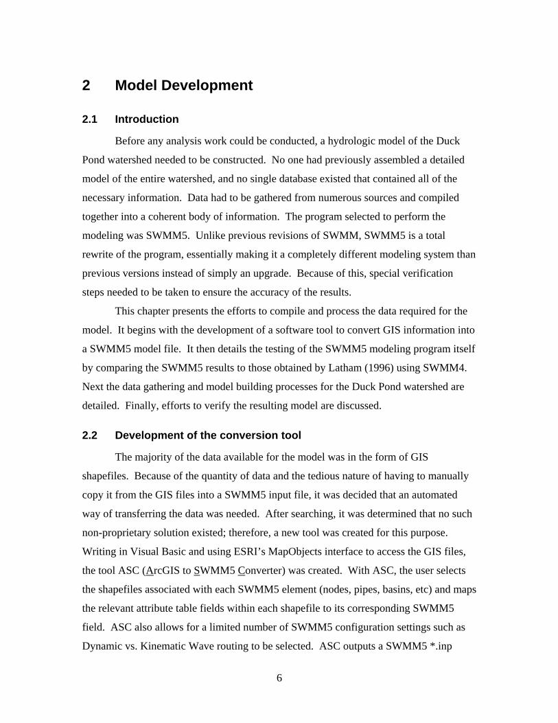
the initial GIS information for the B-lot. As given, the B-lot was divided into 43

subcatchments, one for each available inlet. This was imported to SWMM5 using the

ASC tool. Figure 2.1 illustrates the resulting model.

8

Figure 2.1 – B-Lot SWMM5 Model

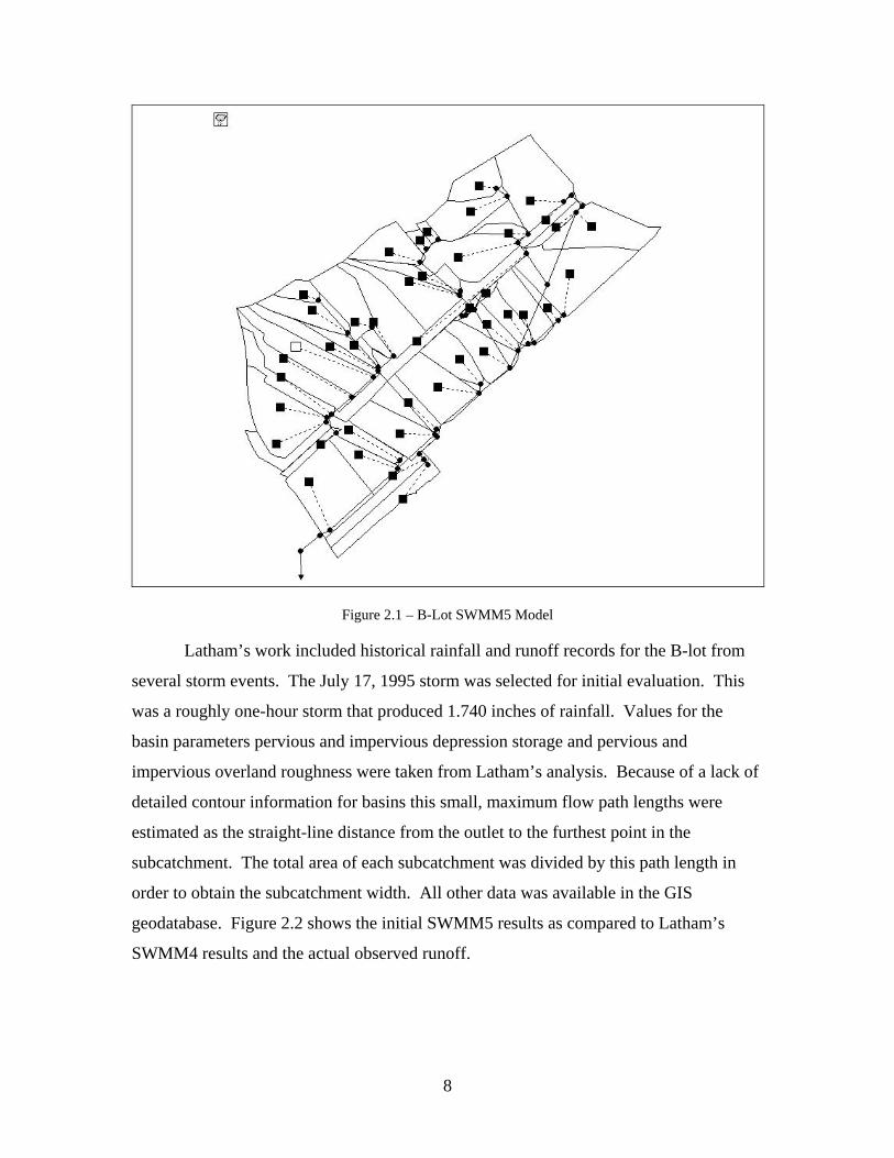
Latham’s work included historical rainfall and runoff records for the B-lot from

several storm events. The July 17, 1995 storm was selected for initial evaluation. This

was a roughly one-hour storm that produced 1.740 inches of rainfall. Values for the

basin parameters pervious and impervious depression storage and pervious and

impervious overland roughness were taken from Latham’s analysis. Because of a lack of

detailed contour information for basins this small, maximum flow path lengths were

estimated as the straight-line distance from the outlet to the furthest point in the

subcatchment. The total area of each subcatchment was divided by this path length in

order to obtain the subcatchment width. All other data was available in the GIS

geodatabase. Figure 2.2 shows the initial SWMM5 results as compared to Latham’s

SWMM4 results and the actual observed runoff.

9

Figure 2.2 – SWMM5 results versus observed runoff for July 17, 1995 storm

0

10

20

30

40

50

60

70

80

0 10 20 30 40 50 60

Time (min)

Flow

(cfs

)

SWMM5SWMM4Observed

10

As can be seen, the peak magnitude and general shape of the SWMM5 outflow

hydrograph match well with the SWMM4 results and the observed results, although the

SWMM5 hydrograph is shifted several minutes earlier. Both the SWMM5 and the

SWMM4 peak results were slightly lower than the observed peak.

Several of the sensitivity checks performed by Latham for SWMM4 were also

repeated in SWMM5. These included varying the number of subcatchments, increasing

and decreasing the basin widths, and increasing and decreasing the percent impervious.

An additional check was also performed regarding the curve number. For the sensitivity

checks, a 1-hour Q10 design storm was used. This storm was generated using

VTPSUHM 6.2 from the Montgomery County IDFs. The following tables illustrate the

results.

Table 2.1 – Basin Width Sensitivity

SWMM5 SWMM4 TPeak QPeak VRunoff TPeak QPeak VRunoff Percent

Change (min) (cfs) (ft3 (x105)) (min) (cfs) (ft3 (x105)) -20% 32 89.84 1.58 43 89.2 1.56 0% 31 95.26 1.59 42 93.5 1.58

+20% 31 99.56 1.59 42 96.7 1.59

Table 2.2 – Percent Impervious Sensitivity

SWMM5 SWMM4 TPeak QPeak VRunoff TPeak QPeak VRunoff Percent

Change (min) (cfs) (ft3 (x105)) (min) (cfs) (ft3 (x105)) -10% 31 88.88 1.48 42 91.1 1.52 0% 31 95.26 1.59 42 93.5 1.58

+10% 32 100.04 1.69 42 93.8 1.63

Table 2.3a – SWMM4 Subcatchment Sensitivity

TPeak QPeak VRunoff Number of Subcatchments (min) (cfs) (ft3 (x105))

1 41 69.5 1.47 6 42 93.5 1.58 12 42 94.6 1.57 42 42 96.4 1.58

11

Table 2.3b – SWMM5 Subcatchment Sensitivity

TPeak QPeak VRunoff Number of Subcatchments (min) (cfs) (ft3 (x105))

9 31 95.26 1.59 43 31 95.26 1.59

As can be seen, the SWMM5 model compared very favorably with SWMM4 both

in peak flow and volume runoff predictions. The primary exception to this would be

SWMM5’s reaction to changes in the percent impervious. In this respect, SWMM5

proved to be significantly more sensitive than SWMM4. The other significant deviation

was in the time to peak. SWMM5 predicted a much shorter time to peak than SWMM4.

Although the SWMM5 model did not directly import the value of its parameters from the

SWMM4 model, none of the differing parameters seem to be able to account for the large

difference in time to peak or the differing reactions to the percent impervious.

Table 2.4 – Curve Number Sensitivity

TPeak QPeak VRunoff Curve Number (min) (cfs) (ft3 (x105))

70 31 94.26 1.57 75 31 95.26 1.59 80 31 96.59 1.61

Varying the curve number from 70 to 80 had very little effect on the runoff peak.

The B-lot was likely not the best site to test the model sensitivity to this variable. This is

because SWMM5 only applies the curve number to the pervious portion of the

subcatchment, and the B-lot is a mostly impervious parking lot. The curve number

results were not compared to Latham’s SWMM4 study because his model used Horton’s

Method for infiltration.

2.4 Data Sources

The data for the complete model was gathered from multiple sources, but it can be

divided into two primary categories: town and campus. Campus data was provided by

S&ID. S&ID had recently commissioned Anderson and Associates to do a detailed

survey of the campus storm sewer system, and the results had been compiled by the

Virginia Tech Center for Geospatial Information Technology (CGIT) into a GIS

12

geodatabase. This geodatabase included all known information about every pipe and

node on campus, as well as detailed subcatchment boundaries and properties. Survey

data had also been collected detailing the cross-sectional transects for open channels as

well as contours for both the Upper and Lower Duck Ponds and the Skelton Pond and

was available in CAD format. The B-lot model used in Section 2.3 was constructed from

a subset of this data.

Data for the town storm sewer system came from a variety of sources. The

primary source was a storm sewer study performed by Hayes, Seay, Mattern and Mattern,

Inc. (HSMM) in 1994 (HSMM, 1994). This study mapped all of the storm water inlets

and pipes in town and compiled the data into a CAD database. Unfortunately important

information such as node inverts was missing from this survey, and the survey did not

identify any storage or detention facilities. The data had also not been updated since its

creation, so significant changes were potentially missing. Even so, this was the most

complete set of data available.

The HSMM data was augmented by three other datasets. First, Blacksburg’s

Town Hall provided the original as-built blueprints for the Upper and Lower Francis

Lane detention ponds located just off of Francis Lane as well as the Collegiate Suites

detention pond located at the corner of N. Main Street and Patrick Henry. Secondly, the

town of Blacksburg performed a stormwater detention pond study in 1998 (Tremel,

1998). The study concentrated on the southern branch of Stroubles Creek, which flows

onto Virginia Tech’s campus near the Graduate Life Center (then the Donaldson Brown

Hotel). It included detailed invert, basin and pipe data for the study area, which had been

compiled into an XP-SWMM model. The Town of Blacksburg made the full report and

all model files available for this research, and S&ID granted permission to use their XP-

SWMM license in order to view the model files. Finally many useful GIS shapefiles

were gathered from the town of Blacksburg website (Blacksburg, 2006). Building

locations, road outlines, two-foot contour maps, land use maps, property boundaries, soil

types, and aerial photographs were all collected for the study area. 10-meter digital

elevation maps (DEMs) used to generate slope maps of Blacksburg were obtained from

the GIS Data Depot (GISDataDepot, 2006).

13

2.5 Data Manipulation

The Duck Pond watershed includes subcatchments, nodes, detention ponds, pipes

and open channel flow. Each of these elements required a number of parameters to be

provided.

2.5.1 Basins

The first step in constructing the model was to delineate the outlines of the entire

Duck Pond watershed. This was done using the two-foot contour map obtained from the

Town of Blacksburg. The resulting watershed was approximately three square miles in

area. This large watershed was then subdivided into two sections: campus and town.

S&ID had already divided the campus section into smaller subcatchments, many of them

far too small to be useful in this study. Using the ArcGIS merge feature, the original 547

campus watersheds provided by S&ID were condensed to 44.

No data existed regarding town watershed boundaries, so the town portion of the

overall watershed was further divided into smaller subcatchments based on the two-foot

contour map. These subcatchments were then adjusted to reflect the location of sewer

pipes and roadways that could direct flows away from their natural paths. In this manner,

the town was divided into 36 subcatchments.

SWMM5 requires the input of a basin width parameter. This parameter provides

SWMM5 with a sense of the geometry of the subcatchment. For a perfectly rectangular

basin, this would be the literal width of the rectangle. For irregular basins, basin width is

generally estimated by dividing the total area of the basin by the length of its longest flow

path. For this study, estimates of the flow path were originally estimated by using

ArcGIS to calculate the straight-line distance from the outlet node of each subcatchment

to the furthest point in the subcatchment. Although presumably this would under-predict

the total length and therefore over-predict the basin width, it was believed that it would

be close enough or would provide a somewhat consistent offset that could be accounted

for by the use of a global multiplier. To test this, the flow paths for several basins were

located by hand using the two-foot contours. These were then compared against the

straight-line estimates. The results showed that there was no consistent pattern of

deviation. Some path lengths were too short and some were too long. Some were only

14

slightly different while others varied drastically. From this it was determined that the

straight-line estimates did not provide reasonable values. The path lengths were therefore

drawn by hand from the two-foot contours for all eighty basins. These path lengths were

then used to calculate the basin widths.

The total percent impervious was calculated differently on campus versus in town.

The campus geodatabase provides a land cover shapefile. In this shapefile, impervious

land cover was given a unique value. An ArcGIS macro was written to calculate the

percent impervious by summing the area occupied by the impervious land cover in each

subcatchment and divide that by the total area of the subcatchment.

In town, the impervious calculation was based on a combination of the road and

building GIS shapefiles and the land use shapefile. The building shapefile contained

polygon outlines of all buildings in Blacksburg. The roads shapefile included all streets

and parking lots in Blacksburg, but it did not include sidewalks or bike paths. The land

use shapefile did not explicitly call out impervious areas; however, some areas were

blank in the file. Through a comparison of the land use shapefile with the road shapefile

and with aerial photography, it was determined that these blank areas corresponded with

the roads, sidewalks and bike paths. These areas were converted to a new land use type

to represent impervious area. The roads, buildings, and land use shapefiles were then

merged to form one file that delineated all of the impervious areas. Using an ArcGIS

macro, these areas were then summed for each subcatchment and used to calculate the

total percent impervious.

The SCS Curve Number approach was used for infiltration simulation. This was

chosen because it had already been selected by S&ID as the method of choice for their

campus simulations, and because of its ease of calculation when provided with land cover

or uses. The S&ID geodatabase included an ArcGIS macro that calculated the curve

numbers for the campus basins based on soil type and land cover. This macro was used

to calculate the curve numbers for the reduced set of campus basins. As previously

mentioned, the town dataset did not include land cover information but did include a land

use shapefile. The original ArcGIS macro was modified so that the calculations for the

town basins would be based on a combination of soil type and land use instead of land

cover. A screenshot of the curve number macro can be found in Appendix A.

15

For both the town and campus curve number calculations, mapping files had to be

created. These files provided the curve number values for each combination of soil type

and land cover or land use. The ArcGIS macro used these tables to produce an area-

weighted average curve number for each basin. For campus, the mapping table supplied

with the geodatabase was used as the basis for calculations. The town land use data was

mapped based upon values suggested by the USDA (1986).

It is important to note that SWMM5 only applies the curve number to the pervious

portion of the subcatchment. This means that if a given curve number is a composite of

the entire site, calculations must be made in order to back out the impervious

contributions. On campus, where the curve number was calculated based on land cover,

impervious areas were simply omitted from the overall calculation, resulting in a curve

number for just the pervious areas. For the town, where the curve numbers were based

on land use, this was more complicated. Each land use category taken from the USDA

was based on an average percent imperviousness for that land use type. That stated

average imperviousness was used to back-calculate the curve number for just the

pervious portion. For example, the USDA lists a ¼ acre residential lot as being on

average 38% impervious. For HSG C, this results in a curve number of 83. By using

38% as the impervious fraction, the pervious curve number is calculated to be

approximately 74. Tables B.1 and B.2 in Appendix B show the curve number mappings

for campus and the town. The town values have been adjusted from the original USDA

values in order to account for the impervious fractions.

The slopes for each basin were determined using a ten-meter DEM

(GISDataDepot, 2006). Using the GIS raster surface analysis tool, a slope map was

generated from the ten-meter DEM. A zonal analysis was then used to calculate the

average slope for each basin.

The remaining basin parameters (pervious/impervious n, pervious/impervious

depression storage, and percent zero impervious) were all set to global values based on

the initial experiments performed on the B-lot or on SWMM5 defaults.

16

2.5.2 Detention Ponds

There were three detention ponds located on campus that were included in this

study: the Upper Duck Pond, the Lower Duck Pond, and the Skelton Pond. Geometric

data was provided for these from S&ID, who had recently commissioned Anderson and

Associates to perform a survey of all ponds and open channels on campus. This survey

data provided detailed contour information for the ponds, from which surface area vs.

elevation charts were derived. Outlet rating curves for the Upper and Lower Duck Ponds

were taken from research performed by Thye (2003).

An outlet rating curve was generated for the Skelton Pond using the Virginia Tech

and Penn State Urban Hydrology Model (VTPSUHM) program. This was based on

direct measurements of the pond’s outlet structure. After generating the curve, the

numbers were compared to the design documents for the pond (“Calculations,” 2003).

The design calculations showed much higher flows for the outlet structure than predicted

by VTPSUHM. It is believe that this is because the design documents assumed inlet

control for all calculations. VTPSUHM estimates that outlet conditions will dominate the

flow, resulting in much lower flowrates. Since the VTPUSHM curve was believed to be

more accurate, it was selected for use in the model.

For the town basins, detention ponds were identified using the two-foot contours.

Numerous areas of depression were identified as likely candidates. These were then

visually inspected in the field. In this manner, seven detention ponds were eventually

located. Each pond was added to the GIS database and established as the outlet of its

own subcatchment.

For each pond, a surface area vs. elevation curve needed to be calculated. The

Town of Blacksburg provided the original construction drawings for the two Francis

Lane ponds and for the Collegiate Suites pond. These documents included one-foot

contour information. From these it was possible to estimate the surface areas at various

elevations, as well as to calculate the minimum and maximum water surface elevations.

For the remaining ponds, the surface area vs. elevation curves as well as minimum and

maximum elevations were calculated using the two-foot contours.

Many of the detention ponds in town had multi-staged outlet structures. Where

possible, detailed measurements of these structures were taken. If the structures were

17

simple enough, they were entered into the model as separate elements. This is true for

ponds that used only a single outlet pipe or a series of orifices or weirs. If the structure

was more complicated, VTPSUHM was used to generate storage-discharge curves.

These were then entered into SWMM5 as outlet structures.

2.5.3 Nodes and Conduits

Campus:

Data for the campus conduits and nodes was taken from the S&ID geodatabase.

As previously mentioned, this database was far more detailed than necessary. All pipes

and nodes above the basin inlet points were omitted. Efforts were also taken to merge

consecutive lengths of similar pipes in order to reduce complexity in the system. In

addition to these simplifications, other data manipulation was also necessary.

In SWMM5 each node must be supplied with an invert and depth value. The

S&ID geodatabase contained detailed surface elevation data for each node, but it did not

include inverts. Invert data had only been taken for the conduits as they entered and

exited a node, and this information was stored in the conduit shapefile. An ArcGIS

macro was written to transfer this data from the conduit shapefile to the node shapefile.

The macro collected the invert information of all pipes entering and exiting each node

and selected the lowest elevation as the node invert. This value was then added to the

node attribute table. Node depth was calculated by subtracting this value from the

surface elevation.

For the campus pipes, the pipe material field had to be mapped to a specific

Manning’s n value. Table 2.5 shows the mapping used.

Table 2.5 – Manning’s n mappings

Code Manning's n Material ADS 0.013 Corrugated Plastic Pipe CMP 0.024 Corrugated Metal Pipe

CONC 0.013 Concrete DIP 0.015 Ductile Iron Pipe

HDPE 0.010 Plastic PVC 0.010 Plastic RCP 0.015 Reinforced Concrete Pipe TCP 0.013 Terracotta Pipe

18

The pipe inlet and outlet offsets from the inlet and outlet nodes also had to be

determined. These values were calculated by subtracting the node invert (as determined

above) from the pipe inlet and outlet inverts supplied in the geodatabase. Because of the

method used to determine the node inverts, this resulted in every node having at least one

incoming or outgoing pipe with an offset of zero.

The campus section also included three open channel reaches. Cross-sectional

transects were obtained for each of these reaches from the survey conducted by Anderson

and Associates. Manning’s n values for the channel and overbank areas were estimated

based on visual inspection and on values recommended by Chow (1959), Palmer (1946)

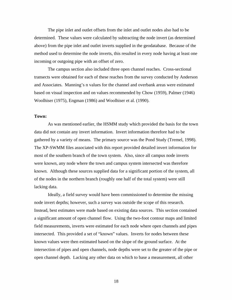
Woolhiser (1975), Engman (1986) and Woolhiser et al. (1990).

Town:

As was mentioned earlier, the HSMM study which provided the basis for the town

data did not contain any invert information. Invert information therefore had to be

gathered by a variety of means. The primary source was the Pond Study (Tremel, 1998).

The XP-SWMM files associated with this report provided detailed invert information for

most of the southern branch of the town system. Also, since all campus node inverts

were known, any node where the town and campus system intersected was therefore

known. Although these sources supplied data for a significant portion of the system, all

of the nodes in the northern branch (roughly one half of the total system) were still

lacking data.

Ideally, a field survey would have been commissioned to determine the missing

node invert depths; however, such a survey was outside the scope of this research.

Instead, best estimates were made based on existing data sources. This section contained

a significant amount of open channel flow. Using the two-foot contour maps and limited

field measurements, inverts were estimated for each node where open channels and pipes

intersected. This provided a set of “known” values. Inverts for nodes between these

known values were then estimated based on the slope of the ground surface. At the

intersection of pipes and open channels, node depths were set to the greater of the pipe or

open channel depth. Lacking any other data on which to base a measurement, all other

19

node depths were arbitrarily set to five feet. During simulation, some node depths were

later increased slightly in order to prevent flooding at those nodes.

The town pipe data also built off of the HSMM study (HSMM, 1994) and the

Pond Study (Tremel, 1998). The HSMM study provided the size, shape and material for

most of the pipes under consideration. When possible, this information was augmented

with data from the Pond Study. The pipe materials were generally mapped to Manning’s

n values according to the values in Table 2.5, but different values were used if provided

by the Pond Study. Pipe entrance and exit offsets were not available, so all offsets were

set to zero.

The town system also contained many open channel reaches. In the southern

branch of town, the Pond Study provided detailed transect and Manning’s n data, but for

the northern branch the data was again lacking. The HSMM report did include some

rudimentary data, but it was over idealized and not current. Instead, field evaluations

were made for each open channel segment. Rough measurements were made by hand

and digital photographs were taken. These were combined with aerial photographs and

the two-foot contours in order to estimate cross-sectional transects and Manning’s n

values.

2.6 Model Generation

After all relevant values had been assigned to both the town and campus datasets,

the two were combined into one unified system GIS database. The ASC tool was then

used to generate the SWMM5 model input file. Figure 2.3 shows the final GIS model.

20

Figure 2.3 – Duck Pond Watershed

2.6.1 Evaporation and Drying Time

In order to use long-term simulations, two more global values need to be set. The

first of these was the drying time. For its infiltration modeling, SWMM5 requires the

input of a drying time. This value represents the number of days necessary for saturated

soil to completely dry. This data was not available for the Duck Pond watershed, so a

general estimate of five days was used.

The second variable was for evaporation. Evaporation removes water from

storage nodes and subcatchment depression storage during dry periods. SWMM5

provides several formats for entering evaporation data. This research used monthly

average values in terms of inches per day. No local data was available, but regional data

21

was in the form of a USDA lysimeter study in Coshocton, OH (McGuinness, 1972).

Table 2.6 shows the values used.

Table 2.6 – Average daily evaporation rates (in/day)

Jan Feb Mar Apr May Jun 0.02 0.04 0.06 0.11 0.20 0.22

Jul Aug Sep Oct Nov Dec 0.22 0.19 0.13 0.08 0.03 0.02

2.6.2 Rainfall Data

Initial design and verification required the use of design storms. 2-, 10- and 100-

year design storms were needed, both of 1 hour and 24 hour duration. The 1-hour storms

were generated using VTPSUHM and the Montgomery County IDF charts. The 24-hour

storm depths were obtained from NOAA Atlas 14 (NOAA, 2006) for the town of

Blacksburg. These values were then used in VTPSUHM to generate 24-hour storm

events according to an SCS Type II curve. Additionally, two more design storms were

created having 1-hour rainfall totals of ½ inch and 1 inch. These were done in

VTPSUHM according to an SCS Type II distribution. The purpose of these storms was

to test various water quality volume rainfall design depths.

Table 2.7 – 1-hour design storm rainfall depths

1/2 Inch 1 Inch Q2 Q10 Q100 Total

Rainfall (in)

0.500 1.000 1.563 2.304 3.206

Table 2.8 – 24-hour design storm rainfall depths

Q2 Q10 Q100 Total

Rainfall (in)

2.76 4.12 6.55

Continuous simulation required the use of long-term hourly rainfall data. Such

data was available from the Roanoke Airport rain gauge for water years (Oct. thru Sept.)

1957-1999. Rather than simulate the entire time period, four representative years were

22

selected. The total rainfall for each water year was tallied and the wettest, driest and

median years were selected. Because BMPs are designed primarily to handle small storm

events, the fourth year was selected because it contained the least number of large storm

events. This was done in an attempt to model a year that would produce maximum BMP

performance results. In calculating the size of storm events, a minimum interevent time

of two hours was used. Table 2.9 details the selected years.

Table 2.9 – Rainfall data for selected water years

DescriptionWater Year

Rainfall Total (in)

Max. Event Total (in)

Dry 1981 25.95 2.65 Average 1992 38.30 3.80

Wet 1987 53.51 6.59 Small 1974 39.09 1.71

2.7 Model Verification

The Duck Pond watershed is not gauged (except for the B-lot), making accurate

model calibration impossible. Since the main focus of this research was to study the

relative effects of BMPs on a system, this lack of calibration does not negatively impact

the results. All tests were conducted relative to a common baseline, even though that

baseline was not calibrated. Previous research by Huber (2002) also showed that

uncalibrated models can still provide useful results as long as long as reasonable

assumptions go into its development. Even so, it was still worthwhile to test the baseline

as much as possible against available data. Although the watershed is ungauged,

previous studies and pond design documentation do provide some predicted (not

measured) results against which the new model could be compared.

Five ponds were used for verification: the Upper and Lower Francis Lane Ponds,

the Skelton Pond, and the Upper and Lower Duck Ponds. For the Francis Lane Ponds

and the Skelton Pond, the original construction documents were available. These

documents predicted the 2-, 10-, and 100-year water surface elevations based on 1-hour

design storms. Thye’s research (2003) provided the predicted water surface elevations

for the Upper and Lower Duck Ponds based on 24-hour design storms events. Since the

23

design storms used in the original calculations were not available, the VTPSUHM-

generated design storms described in section 2.6.2 were used instead.

Table 2.10 – Upper Francis Lane Pond

Return Surface Elevation (ft) Period Design SWMM5 Difference2-year 2078.45 2078.71 -0.26

10-year 2079.25 2080.17 -0.92 100-year 2079.98 2082.04 -2.06

Table 2.11 – Lower Francis Lane Pond

Return Surface Elevation (ft) Period Design SWMM5 Difference2-year 2075.26 2075.83 -0.57

10-year 2076.35 2077.12 -0.77 100-year 2077.46 2078.24 -0.78

Tables 2.10 and 2.11 show the results for the Upper and Lower Francis Lane

Ponds. As can be seen, the two numbers agree well for the 2-year storm event. Both are

starting to depart from the design documents at the 10-year level. At the 100-year level,

the lower pond still performs reasonably well, but the upper pond is off by over two feet.

These ponds are fed by two hydrologically isolated basins, with the upper pond draining

into the lower pond. Storm sewer data was virtually non-existent for the basins, so it is

possible that the flow is not divided correctly in the model between the two ponds or that

surface area currently contributing to the ponds’ inflow is actually being directed to

another outlet. The subcatchments could have also experienced further urbanization

since the original design.

Table 2.12 – Skelton Pond

Return Surface Elevation (ft) Peak Flow In (cfs) Peak Flow Out (cfs)Period Design SWMM5 Difference Design SWMM5 Design SWMM5 2-year 2025.84 2025.93 -0.09 82.73 92.61 0 19.46

10-year 2026.50 2027.18 -0.67 115.35 140.66 20.38 24.63 100-year 2027.91 2028.98 -1.06 207.23 212.06 57.84 28.30

For the Skelton Pond, the surface elevations were reasonably consistent across the

2- and 10-year events, and were off by slightly over a foot for the 100-year event. The

Skelton Pond receives the drainage from just the B-lot and the Skelton Conference

24

Center, so it is an isolated basin. As can be seen, the predicted and design inflows were

relatively similar, differing the most at the 10-year level. For the outflows, the design

documents assumed no flow through the water quality orifice, resulting in the zero design

flow for the 2-year event. As mentioned in section 2.5.2, the design documents also

assumed inlet control for the outlet rating curve whereas VTPSUHM predicted outlet

control. This resulted in much higher design outflows for the 100-year storm than

predicted by either VTPSUHM or SWMM5. This discrepancy in the outflow is the most

likely cause of the difference in surface elevations.

Table 2.13 – Upper Duck Pond

Return Surface Elevation Period Design SWMM5 Difference 2-year 2025.10 2024.35 0.75

10-year 2025.45 2024.40 1.05 100-year 2025.56 2024.42 1.14

Table 2.14 – Lower Duck Pond

Return Surface Elevation Peak Flow In (cfs) Period Design SWMM5 Difference Design SWMM5 2-year 2022.00 2021.58 0.42 1102 813

10-year 2022.90 2021.75 1.15 2450 924 100-year 2023.50 2021.88 1.62 3639 1040

All elevations for the Upper and Lower Duck Ponds were off by significant

amounts. Only the 2-year storm showed less than a foot of difference. In all cases,

SWMM5 predicted surface elevations that were below the reference points. For the

Lower Duck Pond, the peak inflow values predicted by SWMM5 were significantly

below those predicted by Thye (2003) using the SCS Unit Hydrograph method.

Since the SCS Unit Hydrograph method takes a lumped approach to watershed

hydrology, a test was conducted to see how the model would behave if the eighty

subcatchments being modeled in SWMM5 were condensed into just one lumped

subcatchment. As a first step in this test the subcatchment parameters for area were

lumped together and compared to the estimates used by Thye. The lumped curve number

was calculated as an area-weighted average. The results are shown in table 2.15. As can

be seen, the three parameters compare very well between the two models.

25

Table 2.15 – Lumped subcatchment parameters

Model Area Impervious CN (mi2)

Thye 2.95 31.9% 81.66 SWMM5 2.93 30.1% 82.51

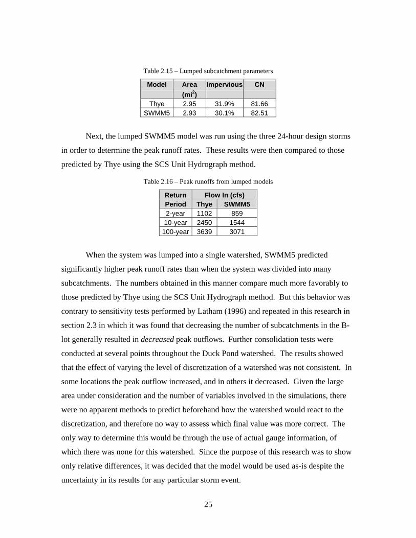
Next, the lumped SWMM5 model was run using the three 24-hour design storms

in order to determine the peak runoff rates. These results were then compared to those

predicted by Thye using the SCS Unit Hydrograph method.

Table 2.16 – Peak runoffs from lumped models

Return Flow In (cfs) Period Thye SWMM5 2-year 1102 859 10-year 2450 1544

100-year 3639 3071

When the system was lumped into a single watershed, SWMM5 predicted

significantly higher peak runoff rates than when the system was divided into many

subcatchments. The numbers obtained in this manner compare much more favorably to

those predicted by Thye using the SCS Unit Hydrograph method. But this behavior was

contrary to sensitivity tests performed by Latham (1996) and repeated in this research in

section 2.3 in which it was found that decreasing the number of subcatchments in the B-

lot generally resulted in decreased peak outflows. Further consolidation tests were

conducted at several points throughout the Duck Pond watershed. The results showed

that the effect of varying the level of discretization of a watershed was not consistent. In

some locations the peak outflow increased, and in others it decreased. Given the large

area under consideration and the number of variables involved in the simulations, there

were no apparent methods to predict beforehand how the watershed would react to the

discretization, and therefore no way to assess which final value was more correct. The

only way to determine this would be through the use of actual gauge information, of

which there was none for this watershed. Since the purpose of this research was to show

only relative differences, it was decided that the model would be used as-is despite the

uncertainty in its results for any particular storm event.

26

3 SWMM 5.0 Before beginning a full discussion of the BMPs considered in this research and

the way in which they were modeled, it is useful to consider the features and limitations

of SWMM5 with respect to BMP implementation. This chapter details many of the

features included with SWMM5 that can be adapted to BMP modeling. More

importantly, it discusses the deficiencies in SWMM5 with respect to BMP modeling and

the strategies employed for dealing with them.

3.1 Quantity Control Features

SWMM5 has a number of features designed to aid in the modeling of BMPs.

These features can generally be broken down into two categories: quantity control and

quality control. The quantity control features will be considered first.

3.1.1 Infiltration

BMPs control quantity through two primary methods: infiltration and overland

flow control. Infiltration is generally accomplished on-site by impounding runoff in a

storage area and allowing it to infiltrate at a designed rate. These impoundments usually

take the form of an infiltration basin or trench. Basins are easily modeled in SWMM5

using a storage node and trenches using an open conduit. Unfortunately SWMM5 only

allows infiltration to occur in subcatchments, not in nodes or conduits. Infiltration BMPs

must therefore be modeled in an indirect manner. This can be accomplished by diverting

the expected infiltration volume into a separate storage node or outfall. This will work,

but it is difficult to achieve precise control over the flowrate. Another method is to use a

pump to simulate the infiltration rate. Pump curves can be devised to mimic the expected

infiltration rate versus hydraulic head behavior. They can also be assigned a steady value

in order to simulate a simple constant infiltration rate. Neither method can account for

changes in infiltration rate due to soil saturation.

It is also possible to model infiltration using subcatchments. SWMM5 allows for

runoff from one subcatchment to flow directly onto another subcatchment. The receiving

subcatchment can be sized to reflect the dimensions of the infiltration basin or trench,

using the depression storage parameter to force the subcatchment to retain the desired

27

infiltration volume. The desired infiltration rate is obtained by manipulating the standard

infiltration parameters using the Green-Ampt method, Horton method, or the SCS Curve

Number method. This is an effective way to fully simulate the characteristics of

infiltration; however, it is difficult to create a subcatchment that accurately reflects the

behavior of a detention basin or a conveyance trench. Also, once flow has entered a

conduit it cannot flow back out onto a subcatchment; therefore, this method could only be

used for runoff flowing directly from an adjacent subcatchment.

3.1.2 Overland Flow

Overland flow control is an important design consideration as it affects the time to

peak, the magnitude of the peak, and the total runoff volume. One method to control

overland flow is to simulate disconnecting the impervious areas from the drainage

network. This allows runoff that would otherwise quickly enter the pipe network with

very little reduction or delay to be greatly slowed and partially infiltrated. SWMM5

allows for this through the use of the Subarea Routing feature. This feature allows runoff

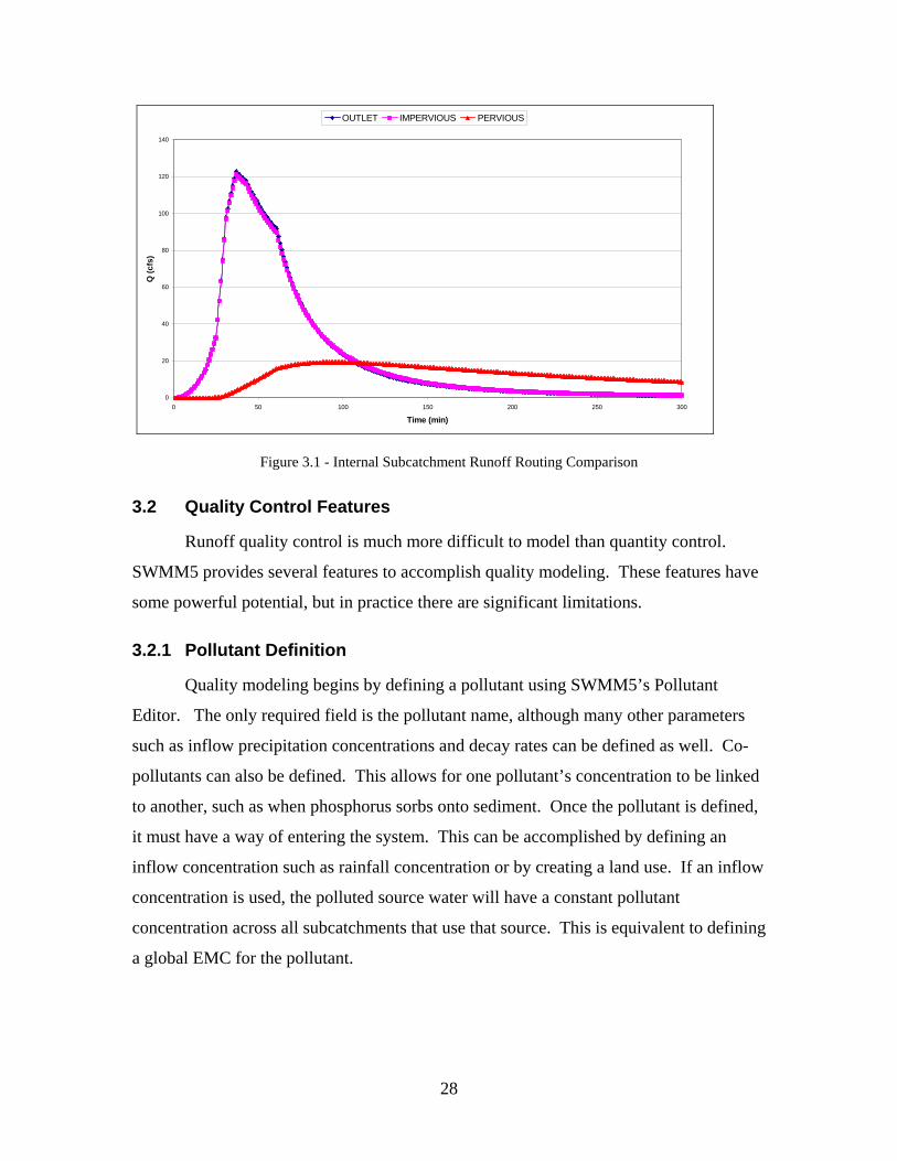
internal to the subcatchment to be routed either from the impervious areas to the pervious

ones (IMPERVIOUS option) or vice versa (PERVIOUS option). Directing the

impervious runoff to the pervious areas before entering the pipes results in significant

peak and volume reduction from an otherwise unchanged subcatchment. This can

simulate BMP practices such as directing rooftop runoff to a grassy field or swale instead

of directly into the storm sewers. By default, SWMM5 uses a third option (OUTLET

option) that drains both the pervious and impervious areas directly into the storm sewer.

In practice this results in very little difference from the IMPERVIOUS option, as it is

generally the runoff from the impervious areas that control the outflow hydrograph.

Figure 3.1 illustrates the results when using these options.

28

0

20

40

60

80

100

120

140

0 50 100 150 200 250 300

Time (min)

Q (c

fs)

OUTLET IMPERVIOUS PERVIOUS

Figure 3.1 - Internal Subcatchment Runoff Routing Comparison

3.2 Quality Control Features

Runoff quality control is much more difficult to model than quantity control.

SWMM5 provides several features to accomplish quality modeling. These features have

some powerful potential, but in practice there are significant limitations.

3.2.1 Pollutant Definition

Quality modeling begins by defining a pollutant using SWMM5’s Pollutant

Editor. The only required field is the pollutant name, although many other parameters

such as inflow precipitation concentrations and decay rates can be defined as well. Co-

pollutants can also be defined. This allows for one pollutant’s concentration to be linked

to another, such as when phosphorus sorbs onto sediment. Once the pollutant is defined,

it must have a way of entering the system. This can be accomplished by defining an

inflow concentration such as rainfall concentration or by creating a land use. If an inflow

concentration is used, the polluted source water will have a constant pollutant

concentration across all subcatchments that use that source. This is equivalent to defining

a global EMC for the pollutant.

29

3.2.2 Land Uses

Land uses provide a range of options when defining the behavior of a pollutant.

A land use is created using SWMM5’s Land Use Editor. The Land Use editor allows for

the definition of specific land uses such as “parking lot” or “lawn.” Land uses allow for

the definition of buildup and washoff functions for each defined pollutant as well as for

the definition of a pollutant EMC. Once a land use is defined, it is applied to a

subcatchment by assigning it to a percentage of the subcatchment’s total area. Any

pollutant buildup and washoff will then be associated with that portion of the

subcatchment. For example, if a land use with a pollutant EMC of 100 mg/l is assigned

to 50% of a subcatchment area, the resulting runoff will contain 50 mg/l, since only half

of the subcatchment was polluted.

The percentage area assignment of a land use results in significant limitations.

Assume a subcatchment is 50% impervious parking lot and 50% grassy lawn, and a land

use named “Parking” has been created to represent the buildup of TSS on the parking lot.

This land use applies only to the parking lot, but SWMM5 only allows for it to be

assigned to 50% of the total subcatchment. This will distribute the land use evenly over

the grassy lawn and the parking lot. Given the differences in runoff behavior between

pervious and impervious areas, this will result in an inaccurate representation of the TSS

behavior. To avoid this, the subcatchments should be broken up so that the parking lot

and the grassy lawn are each completely contained by their own subcatchments. The

Parking land use can then be assigned to 100% of the parking lot subcatchment.

Although generally workable this can be awkward when modeling a large mixed-cover

area.

3.2.3 Pollutant Treatment

SWMM5 provides a variety of methods to simulate treatment. Land uses can be

assigned treatment abilities using street sweeping or BMP efficiencies, which allow for a

percentage removal of pollutants from internal subcatchment flows or from run-on.

Unfortunately, these methods are subject to the same limitations of distribution within the

subcatchment as described above.

30

The primary option for pollution removal is the assignment of treatment nodes.

Any node in the system can be assigned a treatment function, allowing them to simulate

anything from natural pollutant removal in a detention pond to a sewage treatment plant.

Treatment functions can be applied to any type of node, including pipe connection nodes,

storage nodes and outfall nodes. Functions are assigned using the Treatment Editor.

These functions can take the form of either a fractional removal or an outflow

concentration, and can be assigned individually for each defined pollutant. SWMM5

provides a number of parameters for use in defining the functions, such as hydraulic

residence time (HRT), simulation time step (DT) and depth (DEPTH). Although useful,

care must be taken to avoid some issues. The hydraulic residence time should not be

used directly as an input. The HRT parameter is affected by the simulation time step,

resulting in different removal values depending on the time step used. This can be

avoided by rewriting the removal equation in terms of particle settling velocity multiplied

by DT and divided by DEPTH (Eq. 3.1). This method, suggested by Lewis Rossman on

the EPA SWMM listserv, provides results that are consistent regardless of the time step

used. Constant outflow concentrations can also be defined that are independent of any

system variables (Eq. 3.2). ( )DEPTHDTeTSSC /** Θ−= (3.1)

TSSC *15.0= (3.2)

C = concentration

TSS = total suspended solids

DT = simulation time step

DEPTH = hydraulic depth

Θ = particle settling velocity

A major issue with using the Equation 3.1 is that although reasonable results can

be obtained, the values used for treatment constants such as settling velocity have little

physical basis (Huber et al., 2005b). For a given site, the numbers can be calibrated to

produce results consistent with what is observed, but these numbers cannot be accurately

predicted beforehand based on any physical values. Despite this limitation, treatment

functions can still be used effectively if proper calibration is performed or if treatment is

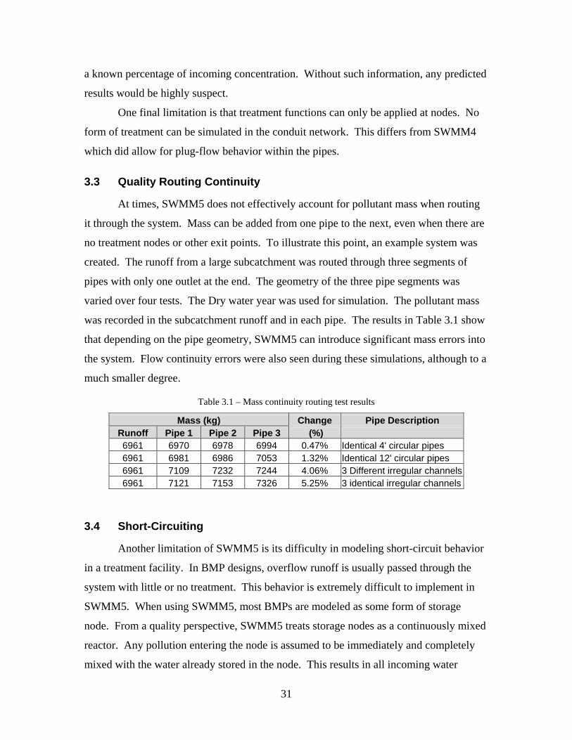
31

a known percentage of incoming concentration. Without such information, any predicted

results would be highly suspect.

One final limitation is that treatment functions can only be applied at nodes. No

form of treatment can be simulated in the conduit network. This differs from SWMM4

which did allow for plug-flow behavior within the pipes.

3.3 Quality Routing Continuity

At times, SWMM5 does not effectively account for pollutant mass when routing

it through the system. Mass can be added from one pipe to the next, even when there are

no treatment nodes or other exit points. To illustrate this point, an example system was

created. The runoff from a large subcatchment was routed through three segments of

pipes with only one outlet at the end. The geometry of the three pipe segments was

varied over four tests. The Dry water year was used for simulation. The pollutant mass

was recorded in the subcatchment runoff and in each pipe. The results in Table 3.1 show

that depending on the pipe geometry, SWMM5 can introduce significant mass errors into

the system. Flow continuity errors were also seen during these simulations, although to a

much smaller degree.

Table 3.1 – Mass continuity routing test results

Mass (kg) Change Pipe Description Runoff Pipe 1 Pipe 2 Pipe 3 (%) 6961 6970 6978 6994 0.47% Identical 4' circular pipes 6961 6981 6986 7053 1.32% Identical 12' circular pipes 6961 7109 7232 7244 4.06% 3 Different irregular channels6961 7121 7153 7326 5.25% 3 identical irregular channels

3.4 Short-Circuiting

Another limitation of SWMM5 is its difficulty in modeling short-circuit behavior

in a treatment facility. In BMP designs, overflow runoff is usually passed through the

system with little or no treatment. This behavior is extremely difficult to implement in

SWMM5. When using SWMM5, most BMPs are modeled as some form of storage

node. From a quality perspective, SWMM5 treats storage nodes as a continuously mixed

reactor. Any pollution entering the node is assumed to be immediately and completely

mixed with the water already stored in the node. This results in all incoming water

32

receiving some level of treatment before exiting the node instead of short-circuiting the

system and flowing through untreated. For BMPs such as infiltration trenches or

bioretention cells where the short-circuiting flows do not significantly mix with the

treated volume, this can result in significant errors. There is no simple way around this.

Either the flows must be divided before they enter the treatment/storage node, or the

treatment must be applied after the flows leave the storage node. After much

experimentation, applying the treatment after leaving the storage node proved to be the

most stable and workable solution. Figure 3.2 illustrates.

Figure 3.2 – Treatment node, including overflow

In this figure, WQO represents a water quality orifice. This is sized to detain the

WQV for a specified amount of time. Any inflow above the WQV should bypass the

system through the Overflow orifice. The WQO is located at the bottom of the storage

node, and the Overflow orifice is located at an offset just above the designed WQV

depth. All treatment is performed at the Treatment node. Node 3 is the normal node

connecting the storage outflow with the rest of the sewer system. Dummy is a dummy

conduit. It does not physically exist, but it is required by the model in order to connect

the treatment node to the normal outflow node. Even though it is a dummy conduit, it

must be given real dimensions or else SWMM5 will generate significant instabilities

during simulation. In this research, Dummy was most often set to fifty feet in length, six

inches to one foot in diameter (depending on flowrates), and a roughness of 0.001 (an

arbitrarily low roughness picked to have as little impact on the flow as possible). It was

also often necessary to offset the storage node, treatment node and node 3 by at least a

tenth of a foot each. In this setup, all flow through the WQO, representing the WQV,

receives full treatment. Flow through the Overflow orifice receives no treatment, thus

33

simulating a short-circuit situation. Testing has shown that overall this setup performs

well, achieving results close to the theoretically predicted values for short-circuiting

situations. This configuration became the basis for many of the BMPs modeled in this

research.

34

4 BMP Identification and Design Before any meaningful tests could be conducted on the system as a whole,

individual BMPs needed to be sited, designed, and modeled. This chapter begins by

detailing the process of selecting potential BMP locations and deciding which type of

BMP if any would be best at each location. The methods used to model each type of

BMP are also described. After examining the list of potential BMPs, a final list is

produced for inclusion in the town model. Variations in these BMPs are then used to

produce four different versions of the town model.

4.1 Initial BMP Selection

Unlike conventional storm water control facilities that attempt to control runoff at

points far downstream, BMPs are generally intended for use closer to the runoff source.

Since the majority of the runoff in the Duck Pond watershed originates in the town of

Blacksburg and not on the Virginia Tech campus, the search for potential BMP locations

only focused on areas within the town. In order to reduce potential installation costs only

properties already owned by the town were considered. Using a GIS shapefile detailing

properties owned by the town, twenty-three initial sites were identified. Each of these

sites was examined to determine whether or not it was a good candidate for a BMP

installation. Five sites were eliminated, leaving eighteen working BMP sites for

evaluation via SWMM5.

Using the BMP design manual created by Young and Kibler (2006) as a

reference, the investigator examined the eighteen sites to determine what BMPs would be

possible. The soil types, average depth to bedrock, average depth to water table, and

average infiltration rates were determined for each site using the Montgomery County

Soil Survey (Creggar, 1985). Most areas were determined to be on average over four feet

above the regional bedrock and groundwater table and to have at least a 0.5 in/hr

infiltration rate in the upper soil layers. This meant that most BMPs types including

infiltration practices would be possible at the selected locations. Based on this data and

without regard for which BMP would be the most appropriate, a comprehensive list of all

candidate BMPs was produced for each of the eighteen sites.

35

Each site was then examined in further detail to determine which of the candidate

BMPs would be the most reasonable and effective. Consideration was now given to the

appropriateness of each potential BMP. Although a site might have several feasible BMP

options, often many were not practical or would be less effective than other options at the

same site. Working in this manner, a final list of BMPs was produced. Most sites were

reduced to only one remaining candidate BMP. Three sites contained separate BMPs

operating in series or in parallel. Three other sites retained two mutually exclusive

BMPs. The final decision for these sites was postponed until after further testing. The

final list contained a variety of potential BMPs including bioretention, infiltration

trenches, infiltration basins, extended dry detention ponds, vegetated roofs, grassed

swales, constructed wetlands, water quality inlets and porous pavement.

4.2 BMP Design and Modeling

Next, each of the identified BMPs had to be designed and modeled. The designs

were based on the examples provided in Young and Kibler’s design manual (2006).

Although there were a total of thirty BMPs, there were only nine different types. The

general design and modeling process used for each type is described in the following

sections. The designs presented below were not performed to the level of detail

necessary to actually construct the BMPs. Since the purpose of this research was simply

to model their relative effects, the designs contained only the information necessary to

implement the model.

4.2.1 Global Design Considerations

4.2.1.1 Water Quality Volume and Drawdown Time

The design WQV was taken to be the first ½ inch of rainfall over the impervious

area, as per VDOT regulations (VDOT, 2004). VDOT also specified a 30-hour

drawdown time for WQV storage.

4.2.1.2 Design for Treatment Function

Two methods were used to model the infiltration practices. The first approach

was to model as closely as possible the theoretical removal rates for the selected BMPs.

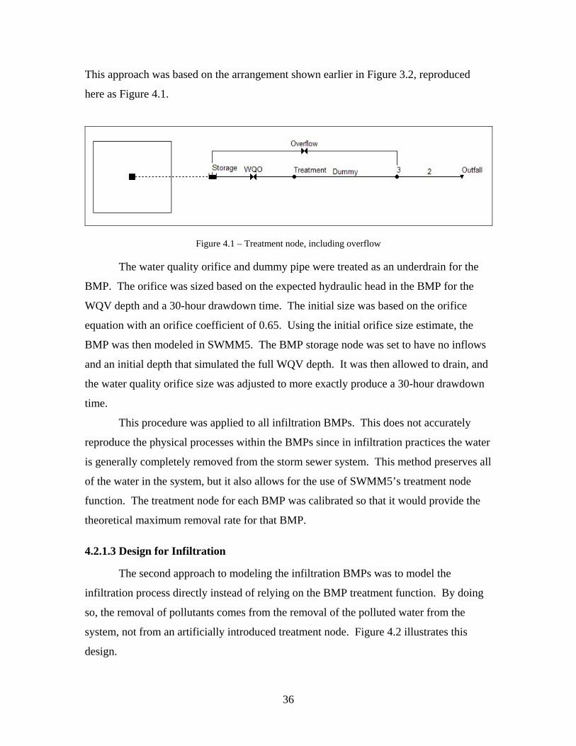
36

This approach was based on the arrangement shown earlier in Figure 3.2, reproduced

here as Figure 4.1.

Figure 4.1 – Treatment node, including overflow

The water quality orifice and dummy pipe were treated as an underdrain for the

BMP. The orifice was sized based on the expected hydraulic head in the BMP for the

WQV depth and a 30-hour drawdown time. The initial size was based on the orifice

equation with an orifice coefficient of 0.65. Using the initial orifice size estimate, the

BMP was then modeled in SWMM5. The BMP storage node was set to have no inflows

and an initial depth that simulated the full WQV depth. It was then allowed to drain, and

the water quality orifice size was adjusted to more exactly produce a 30-hour drawdown

time.

This procedure was applied to all infiltration BMPs. This does not accurately

reproduce the physical processes within the BMPs since in infiltration practices the water

is generally completely removed from the storm sewer system. This method preserves all

of the water in the system, but it also allows for the use of SWMM5’s treatment node

function. The treatment node for each BMP was calibrated so that it would provide the

theoretical maximum removal rate for that BMP.

4.2.1.3 Design for Infiltration

The second approach to modeling the infiltration BMPs was to model the

infiltration process directly instead of relying on the BMP treatment function. By doing

so, the removal of pollutants comes from the removal of the polluted water from the

system, not from an artificially introduced treatment node. Figure 4.2 illustrates this

design.

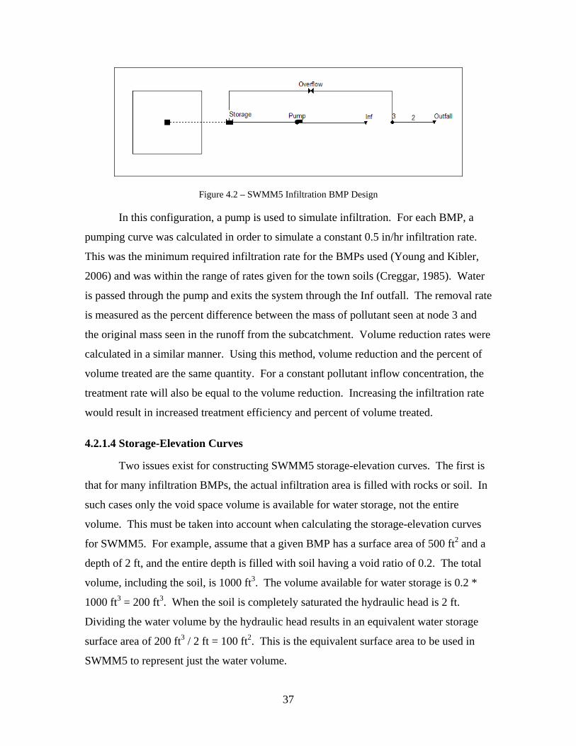
37

Figure 4.2 – SWMM5 Infiltration BMP Design

In this configuration, a pump is used to simulate infiltration. For each BMP, a

pumping curve was calculated in order to simulate a constant 0.5 in/hr infiltration rate.

This was the minimum required infiltration rate for the BMPs used (Young and Kibler,

2006) and was within the range of rates given for the town soils (Creggar, 1985). Water

is passed through the pump and exits the system through the Inf outfall. The removal rate

is measured as the percent difference between the mass of pollutant seen at node 3 and

the original mass seen in the runoff from the subcatchment. Volume reduction rates were

calculated in a similar manner. Using this method, volume reduction and the percent of

volume treated are the same quantity. For a constant pollutant inflow concentration, the

treatment rate will also be equal to the volume reduction. Increasing the infiltration rate

would result in increased treatment efficiency and percent of volume treated.

4.2.1.4 Storage-Elevation Curves

Two issues exist for constructing SWMM5 storage-elevation curves. The first is

that for many infiltration BMPs, the actual infiltration area is filled with rocks or soil. In

such cases only the void space volume is available for water storage, not the entire

volume. This must be taken into account when calculating the storage-elevation curves

for SWMM5. For example, assume that a given BMP has a surface area of 500 ft2 and a

depth of 2 ft, and the entire depth is filled with soil having a void ratio of 0.2. The total

volume, including the soil, is 1000 ft3. The volume available for water storage is 0.2 *

1000 ft3 = 200 ft3. When the soil is completely saturated the hydraulic head is 2 ft.

Dividing the water volume by the hydraulic head results in an equivalent water storage

surface area of 200 ft3 / 2 ft = 100 ft2. This is the equivalent surface area to be used in

SWMM5 to represent just the water volume.

38

The second issue is the conversion of volume increments to equivalent surface

areas. SWMM5 requires that storage curves be recorded as surface area vs. elevation, but

in many designs in this research it was the volume increment that was known, not the

surface area. Internally, SWMM5 uses the following equations to calculate volume from

surface area.

0ddd −=Δ (4.1)

01

01

ddSASAm

−−

= (4.2)

dmSASA Δ+= 0 (4.3)

2)( 2

00dmdSAVV Δ

+Δ+= (4.4)

d0 = Depth at the start of the step

d1 = Depth at the end of the step

d = Depth between d0 and d1 at which the surface area and volume are being interpolated

m = Slope of the change in surface area between depths d0 and d1

SA0 = Surface area at depth d0

SA1 = Surface area at depth d1

SA = Interpolated surface area at depth d

V0 = Volume at depth d0

V = Interpolated volume at depth d

Equation 4.3 is a straight-line interpolation of the surface area at the requested

depth. Equation 4.4 is an integration of 4.3 with respect to depth. Using these equations,

it is possible to calculate what surface area is required in order to force SWMM5 to

calculate the correct volume at a given depth. Although the algorithm is relatively

intuitive, the surface areas it generates often are not. Returning to the previous example

of the 2 ft basin filled with soil, now assume there is an additional 0.5 ft of open-air

storage above the soil layer. Since the total surface area of the basin is 500 ft2 the volume

of the open-air storage is 250 ft3. In order to remove the soil volume, the equivalent

surface area for the first two feet should be 100 ft2 as calculated previously. But if the

surface area at 2 feet is set to the equivalent value of 100 ft2 and the surface area at 2.5

39

feet is set to the actual value of 500 ft2, equation 4.4 will calculate a volume increment of

only 150 ft3. The surface area needed to obtain the actual volume increment of 250 ft3 is

back calculated to be 900 ft2. Tables 4.1 and 4.2 illustrate the differences.

Table 4.1 – Actual surface area vs. depth curve, including soil

Depth (ft) Area (ft2)0 500 2 500

2.5 500

Table 4.2 – Surface area vs. depth curve, adjusted to remove soil volume

Depth (ft) Area (ft2)0 100 2 100

2.5 900

When going from 2 ft to 2.5 ft at a constant surface area of 500 ft2 in table 4.1,

SWMM5 will correctly calculate the volume increment to be 250 ft3. When moving

from 2 ft at 100 ft2 to 2.5 ft, the new surface area of 900 ft2 is required. Using the

numbers in table 4.2, equation 4.4 will now calculate the correct volume increment of

250 ft3. This kind of calculation came into play on all BMPs where the storage was split

between a void-space section and an open-air section.

4.2.2 Bioretention

A bioretention BMP is essentially a small infiltration basin consisting of a

specially engineered soil matrix and plant mixture. Treatment primarily occurs due to

adsorption, infiltration and biological decomposition. They are often located in parking

lot islands or just beside large impervious areas. They make excellent complements to

parking lots or roadways as they generally take advantage of existing pervious

landscaping areas and make them into functional units. As a general sizing guideline, the

surface area of the treated impervious area should not be more than five times the surface

area of the bioretention cell. The engineered soil depth should be at least two feet, with a

maximum of six inches of open-air storage available above the soil. (Young and Kibler,

2006)

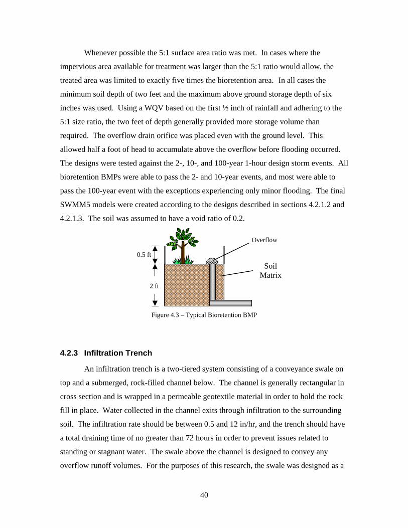
40

Whenever possible the 5:1 surface area ratio was met. In cases where the

impervious area available for treatment was larger than the 5:1 ratio would allow, the

treated area was limited to exactly five times the bioretention area. In all cases the

minimum soil depth of two feet and the maximum above ground storage depth of six

inches was used. Using a WQV based on the first ½ inch of rainfall and adhering to the

5:1 size ratio, the two feet of depth generally provided more storage volume than

required. The overflow drain orifice was placed even with the ground level. This

allowed half a foot of head to accumulate above the overflow before flooding occurred.

The designs were tested against the 2-, 10-, and 100-year 1-hour design storm events. All

bioretention BMPs were able to pass the 2- and 10-year events, and most were able to

pass the 100-year event with the exceptions experiencing only minor flooding. The final

SWMM5 models were created according to the designs described in sections 4.2.1.2 and

4.2.1.3. The soil was assumed to have a void ratio of 0.2.

Figure 4.3 – Typical Bioretention BMP

4.2.3 Infiltration Trench

An infiltration trench is a two-tiered system consisting of a conveyance swale on

top and a submerged, rock-filled channel below. The channel is generally rectangular in

cross section and is wrapped in a permeable geotextile material in order to hold the rock

fill in place. Water collected in the channel exits through infiltration to the surrounding

soil. The infiltration rate should be between 0.5 and 12 in/hr, and the trench should have

a total draining time of no greater than 72 hours in order to prevent issues related to

standing or stagnant water. The swale above the channel is designed to convey any

overflow runoff volumes. For the purposes of this research, the swale was designed as a

0.5 ft

2 ft

Overflow

Soil Matrix

41

trapezoidal channel with 3:1 side slopes. Infiltration trenches should only be used for

drainage areas of ten acres or less. (Young and Kibler, 2006)

As mentioned in chapter 4, SWMM5 does not allow infiltration from conduits.

The trench was therefore modeled according to the methods put forward in sections

4.2.1.2 and 4.2.1.3. A storage node was created to simulate the storage capacity of the

total trench, including the rock infiltration channel and the swale. An overflow orifice

was located just above the volume contained by the rock infiltration channel. In order to

verify that this configuration could accurately reproduce the flow characteristics of an

actual trench, comparison tests were made. An irregular channel was designed that fit the

dimensions of the infiltration trench. A weir was placed at the outlet of this channel with

the crest located at the top of the rock infiltration channel. The flow characteristics of

this system were then compared to those of the storage system. Although there were

some minor differences, the two compared very favorably.

In calculating the storage-elevation curve equivalent for the infiltration trench,

care had to be taken to avoid the issues described in section 4.2.1.4. A void ratio of 0.4

was used to calculate the water storage volume of the rock fill. The base of the

trapezoidal channel was assumed to be the same as the width of the rock trench.

Figure 4.4 – Infiltration Trench

4.2.4 Infiltration Basin

When the drainage area is too large for an infiltration trench, an infiltration basin

may be used. Infiltration basins are basically detention ponds with the lowest overflow

outlet located above the WQV depth. The WQV only exits the basin through infiltration.

Rock

Surface

Permeable

Underdrain

42

All incoming flows above the WQV bypass the system through an overflow structure.

The basin should completely drain in 72 hours or less in order to avoid health issues

associated with standing water. A minimum depth must exist between the bottom of the

basin and the local water table and bedrock. Care should also be taken to ensure that the

infiltrated water does not destabilize any nearby building foundations. All flows entering

the basin should be first directed to either a filter strip or a sediment forebay in order to

minimize pore clogging and sediment buildup in the basin. Infiltration basins can be

combined with extended dry detention ponds by using a multi-staged riser box for the

outlet structure. (Young and Kibler, 2006)

Two infiltration basins were used in this research. In both cases the incoming

flows naturally pass over grassed areas or through other BMPs, providing the required

prefiltering. Because of the limited space and in order to simplify the design, no attempt

was made to detain the overflow volumes. Anything above the WQV was designed to

pass through the overflow structure. No on-site attempt was made to verify that the local

geologic conditions would support an infiltration basin. Data gathered from the

Montgomery County Soil Survey (Creggar, 1985) suggests that on average the

Blacksburg area can support such structures, but before any actual construction begins

each site would have to be examined in detail to determine its appropriateness. The

SWMM5 storage-elevation curves were based on the existing land topography. The final

basins were modeled according to the orifice and infiltration methods put forward in

sections 4.2.1.2 and 4.2.1.3.

4.2.5 Grassed Swale

A grassed swale performs two purposes. First, it conveys storm water. Second, it

slows down the flow in order to allow for quality improvements through sedimentation

and filtration. Grassed swales are often used in series with other BMPs as a prefilter. A

swale is generally a trapezoidal channel with a bottom width less than eight feet. Greater

widths tend to concentrate flows, negating the benefits of the swale. Check dams are

used in order to achieve the necessary detention time to allow for sedimentation. These

check dams should be a maximum of eighteen inches in height. The swale above the

43

check dams should be high enough to allow for the 10-year storm to pass with at least six

inches of freeboard. (Young and Kibler, 2006)

Only one grassed swale was used in the model. Rather than serve as a prefilter,

the grassed swale was located at the outlet of a small detention pond. It has questionable

value at such a location, but it was kept for the sake of evaluation. Since its source

subcatchment was rather large, the swale was unable to handle the full WQV. Instead it

was designed to handle approximately one tenth of the WQV. The maximum bottom

width of eight feet and check dam height of eighteen inches were used. The final channel

was 2.25 feet in depth. This passed the 10-year event with the required freeboard and

passed the 100-year event with only minor flooding.

The storage capacity of the swale was modeled using a storage node. Because the

swale was a part of the conveyance system and was located at the outlet of a detention

pond, the actual trapezoidal channel had to be included as well. This was modeled as an

open trapezoidal section connecting the outflow of the detention pond with the storage

node. Because the storage node accounted for the storage created by the check dams, the

check dams themselves were not modeled. A test was conducted where the channel was

broken into segments and weirs were used for check dams. The flow through this system

was compared to the flow through the single unobstructed trapezoidal channel and

storage node model. The results were nearly identical; therefore, the much simpler

channel and storage node option was selected.

The outflow from the storage node was designed according to the method

described in section 4.2.1.2. The theoretical treatment efficiency was assigned to the

treatment node; however, since the swale was not designed to treat the full WQV, the

overall BMP efficiency will be much lower. The expected overall theoretical value was

scaled to reflect the volume expected to bypass even during normal conditions.

4.2.6 Porous Pavement

A porous pavement system is generally designed to have a top layer of porous

asphalt or concrete located above an aggregate-filled basin. The basin is usually sized to

hold the full 2-year event, not just the normal WQV. The water stored in the reservoir is

infiltrated into the surrounding soil. A minimum depth must exist between the bottom of

44

the reservoir and the local water table and bedrock. Care should be taken to ensure that

the infiltrated water does not destabilize any nearby building foundations. Storms larger

than the 2-year event must be conveyed away from the site. This can be accomplished

through the use of an underdrain or by allowing the excess water to flow across the

surface of the pavement to a conventional stormwater facility. Porous pavement is most

often used in parking lots. The system captures all rainfall on its surface. Roof runoff

and gutters from nearby buildings can also be directed to the pavement reservoir. (Young

and Kibler, 2006)

The porous pavement BMPs used in this research were modeled according to the

treatment and infiltration methods described in sections 4.2.1.2 and 4.2.1.3. They were

designed to hold the full 2-year 1-hour storm event, which was estimated using the design

storm generated by VTPUSHM to be 1.56 inches. All of the systems were parking lot

retrofits. Some treated just the parking lot runoff while others were able to accept

additional runoff from nearby buildings. Overflow was handled by a perforated pipe

located above the reservoir but below the pavement surface. This effectively added the

diameter of the pipe to the reservoir depth. The reservoir was filled with stone aggregate

with a void ratio of 0.4. This void ratio was used to calculate the storage-elevation curve

as described in section 4.2.1.4 with the overflow pipe layer treated as open air. Testing

with both the infiltration and orifice versions of the design generally resulted in the BMPs

being able to infiltrate both the 2 and the 10-year events, with overflow only occurring at

the 100-year level.

4.2.7 Vegetated Roof

A vegetated roof consists of several layers. At its simplest, the roof must contain

a base waterproof layer, an engineered water storage media layer, a growth media layer,

and carefully selected vegetation. Roof covers as thin as six inches can achieve

significant peak and volume reductions, although the actual reduction amount is highly

dependent upon the materials used. Quality improvements are less obvious since roofs

will not experience the same pollutant buildup as a parking lot or road. It is important

that the vegetated roof be properly drained in order to prevent standing water or damage

to the building. (Young and Kibler, 2006)

45

Because of the variability in the effects of a vegetated roof due to the design and

materials used, it is hard to accurately model them in the absence of detailed design

information. A general method suggested by the Pennsylvania Department of

Environmental Protection is that “for storm events in which the total rainfall depth is no

more than three times the maximum media water retention for the assembly, the rate of

runoff from the roof will be less than or equal to that of open space” (PADEP, 2005).

This was the approach taken for this research. The curve number for open space in good

condition with soil of type HSG C is 78 (Mayes, 2005). To model a vegetated roof

within a subcatchment, the impervious area of the roof was replaced with an equivalent

sized pervious area with a curve number of 78. Quality benefits were not calculated.

4.2.8 Constructed Wetlands

Wetlands are shallow marshes that provide water quality treatment through

physical, biological and chemical processes. A sediment forebay should exist to control

the amount of sediment entering the system. The permanent wetland consists of three

sections: a shallow area six inches or less in depth, an intermediate area eighteen inches

or less in depth, and a deep pool. The shallow area should occupy about 35% of the

wetland surface area. The intermediate pool should be 65% of the surface area, including

the shallow pool area. The total wetland area should be at least 1% of the contributing

area. At least four feet of storage should be available above the permanent pool. (Young

and Kibler, 2006)

Unlike other BMP locations where the water table needed to be far below ground,

a constructed wetland requires either a shallow water table or permanent baseflow. One

area was located in Blacksburg that was an ideal candidate for a constructed wetland.

The site was located beside a major tributary of Stroubles Creek and backed into a

hillside that appeared to intersect the groundwater table. A detailed water budget was not

conducted for the area, but continuous flow was observed on multiple occasions

throughout the year during both dry and wet periods. No other inflows into the area were

apparent. A small natural wetland already existed at the site.

The drainage area contributing to the tributary was far greater than the wetland

could handle. The wetland could reasonably treat only about 2% of the total contributing

46

area. The WQV calculation was based on that 2% area, with imperviousness held the

same as for the entire subcatchment. The wetland surface area was taken to be 2% of the

reduced drainage area. The wetland’s shallow, intermediate and deep pools were sized

based on the previously stated criteria. The area above the permanent pool was given a

maximum depth of four feet.

For modeling purposes, the permanent pool was not included. This is because for

individual storm events, having a pre-existing permanent pool drastically affected the

water quality results. The initial water in the permanent pool was completely clean. The

incoming polluted water would mix with the clean water, artificially inflating the removal

percentage and making it impossible to calibrate the treatment node to provide the

desired level of treatment.

The wetland was designed as an offline facility. A diversion orifice located on

the main tributary diverted the approximate WQV to the wetlands. Any flows beyond the

WQV immediately exited the wetlands through the bypass structure. Figure 4.5 shows

the final SWMM5 model used.

Figure 4.5 – SWMM5 Model of a Wetland BMP

Node 5 represents the inflow of the main tributary. Flow passes through the

Diversion orifice into the wetland and rejoins the main tributary at node 3. Unlike many

other BMP devices in this research all treatment occurs in the storage node, affecting the

overflow as well as the WQV. In the other BMPs where the two flows are diverted

before treatment, the treatment occurs in a zone that is significantly different than the

overflow area. For bioretention the treatment zone is filled with soil; for porous

pavement, the treatment zone is filled with rock. In these cases, the treatment zones

47

behave differently than the overflow zones. For the wetlands, the treatment zone and

overflow zone are the same. Although short-circuiting will occur, some mixture will also

occur. The final result would likely be between the two extremes of separation or not.

Since neither method was clearly more correct than the other, the simpler approach was

taken.

4.2.9 Water Quality Inlets

Water quality inlets come in a variety of forms, but they all function in the same

basic manner. A filter is inserted into a drop inlet. This filter is designed to treat a

portion of the inflow and bypass any flows above that amount. Water quality inlets have

the advantage of providing good treatment benefits while also being cheap and easy to

install and maintain. (Young and Kibler, 2006)

Water quality inlets are proprietary devices produced by many different

companies. Each has its own design, resulting in varying maximum treatment and

overflow loads. Inlets are chosen based on their filtering and overflow capacity. Many

are custom made to fit standard drop inlet sizes. The water quality inlet chosen as a basis

for this research was the FloGard+Plus model FF-1824D from KriStar Enterprises. This

model has a maximum filtered flow of 1.1 cfs and an overflow capacity of 0.6 cfs. This

amount was deemed sufficient to handle the runoff from the selected sites. This model

was chosen primarily because good treatment efficiency and pricing data were available

(MaSTEP, 2004).

Figure 4.6 – SWMM5 Model of a Water Quality Inlet

48

As can be seen in Figure 4.6, the water quality inlet model required a different

approach than the other BMPs. Because water quality inlets do not use a storage node,

the method presented in section 4.2.1.2 to separate the treated and overflow portion of the

flows was not applicable. For water quality inlets, the flow separation needed to be based

on flowrates. Although SWMM5 provides a flow divider object that can accomplish this,

it can only be used under kinematic wave routing, not dynamic wave routing. The

division was instead accomplished through the use of SWMM5’s control rule feature.

Control rules allow the modeler to dynamically adjust system controls in one location

based on conditions at another location. When flow in the incoming conduit was below

1.1 cfs, the control rules instructed the Treated orifice to be completely open and the

Bypass orifice to be completely closed. When the incoming flow became greater than 1.1

cfs, the Treated orifice was closed and the Bypass orifice was opened. Although this

method forced the inflows to be completely treated or completely bypassed, further

refinement is possible. The control rules allow for the orifices to be only partially opened

or closed. Through testing this could allow for bypass and treated flows to co-exist, but

since the water quality inlets were not chosen for inclusion in the final system model this

step was not taken.

4.2.10 Extended Dry Detention Pond

Extended dry detention (EDD) ponds are adaptations on a traditional detention

pond. Whereas traditional detention ponds are only designed to regulate peak outflow,

EDD ponds are designed to hold the WQV for a specific period of time. Any flows

above the WQV may or may not be regulated. Detaining the WQV for an extended

period of time allows for sedimentation of suspended pollutants. It can also reduce and

delay the outflow peak.

Two EDD ponds were designed for the Blacksburg system, one on the north

branch of Stroubles Creek and one on the south branch. Each was located at a point in

the watershed where it received far more flow than could be contained in the volume

available. Each pond was therefore designed to hold only as much as possible. Because

of the limited space, flow above the treated volume was immediately bypassed. Since the

entire WQV was not detained, the treatment percentages were reduced to reflect the

49

volume that actually received treatment. The shape of the ponds came from the existing

contours of the land. With excavation, more storage volume could be achieved. As

described in section 4.2.8 for wetlands, the treatment function was applied to the storage

node itself. Both the bypass flow and the WQV received treatment, although the bypass

volume to a lesser degree since it spends less time in storage.

4.3 Final BMP Selection

With each candidate BMP designed and tested individually, the next step was to

finalize the list of BMPs to be included in the model. As previously mentioned several

sites were modeled with multiple competing BMPs. The decision was made that when

two or more potential BMPs were mutually exclusive, the BMP with the largest potential

impact on the system would be selected. This was done in order to maximize the system-

wide impacts of the local BMPs. As a result porous pavement was selected over the

water quality inlets, eliminating the inlets from the final model. Porous pavement also

took the place of two bioretention cells. The two EDD ponds were also not included in

the final model, despite having significant potential to show benefits at the system level.

This was done for two reasons. First, one goal of this research was to see the potential

impacts of local BMPs at the large-scale system level. The EDD ponds were regional

facilities, not local ones, and were both located downstream of the local BMPs. They

produced much larger effects than the local BMPs and were therefore capable of masking

any noticeable effects from the local BMPs. Secondly, the EDD ponds experienced

significant backwater conditions when inserted into the town model. These backwater

conditions made it virtually impossible to obtain an accurate measurement of the amount

of pollutant removed.

The final BMPs were then inserted into the system model. In most cases, the

BMP’s contributing area was extracted from its original subcatchment and converted into

its own separate subcatchment with the BMP as its outlet. The BMPs were then

connected to the existing storm sewer network. Vegetated roofs were inserted by

replacing the impervious area of the subcatchment with a pervious area with a curve

number of 78. The grassed swale and constructed wetland were placed within the

50

existing conveyance system. Maps in Appendix B show the types and locations of all

final BMPs.

4.4 Model Versions

In order to test different aspects of the BMPs, four versions of the final system

model were produced. Each included the same list of BMPs and was modeled based on

the principles already described in this chapter.

4.4.1 Treatment Node Model

In this version of the model all bioretention, infiltration basins, infiltration

trenches and porous pavement BMPs were modeled according to the principles described

in section 4.2.1.2. Each BMP was sized based on the recommendations taken from

Young and Kibler (2006). This meant that many final BMP designs were capable of

treating more then just the half-inch WQV. The treatment nodes were calibrated based

on just the WQV, not the maximum volume the BMPs were capable of treating.

The goal of this model was to test the effectiveness of the BMPs when designed

according to specifications. By using the treatment nodes to force the treatment

percentages to the published values, the model should experience a best-case scenario.

This should result in maximum treatment for rainfall values at or below the WQV;

however, throughout a given year rainfall values larger than half an inch will occur or

events may occur in rapid succession, with a new event arriving before the BMP has

completely recovered from the previous event. These situations will degrade the overall

performance of the BMPs. After simulation, the final results will be examined for the

entire system as well as for each individual BMP. Each BMP’s performance will be

evaluated and compared to the published efficiencies.

4.4.2 Infiltration Model

In this version of the model all bioretention, infiltration basin, infiltration trench,

and porous pavement BMPs were based on the design principles in section 4.2.1.4. In all

other respects, it was identical to the treatment node model. All BMP sizes were

unchanged.

51

The goal of this model was to test the accuracy of the published removal

percentages for each infiltration BMP by modeling the primary treatment process itself

(infiltration) rather than simply forcing the treatment to the published results. The results

for each individual BMP are compared to the results obtained with the treatment node

model and to the published treatment efficiencies.

4.4.3 Half-Inch and One-Inch Models

The final two versions of the model were each based on the Infiltration model.

The difference was the sizing of the BMPs themselves. Ignoring the sizing guidelines in

Young and Kibler’s design manual (2006), each infiltration BMP was resized to hold

exactly the WQV. For example, in the original design each bioretention BMP soil depth

was set to two feet regardless of what was necessary to hold the required WQV. The

overflow drain was located on the surface of the soil at two feet. As an example, assume

that in the Infiltration model the WQV filled a particular bioretention BMP to a depth of

1.6 feet, but the soil depth was still set to 2 feet. For these two new versions of the model,

the depth of the soil would be changed to 1.6 feet, with the overflow drain located on the

new soil surface. The BMPs in the Half-Inch and One-Inch models were resized using a

½ inch and 1 inch WQV, respectively.

The purpose of these models was to test the accuracy of the half-inch rule in

determining WQV. In 1983 the Nationwide Urban Runoff Program, conducted by the

EPA, proposed that capturing the first half-inch of runoff would result in treating

approximately 90% of the total runoff. This was based on the idea that the majority of

storm events are small in nature, and that a high concentration of the overall pollutants

would be in the first flush. Since this initial report, many areas have required higher

values, even going as high as 1.25 inches (PADEP, 2005). The Half-Inch and One-Inch

models were designed to test these assertions for the Blacksburg area. Each BMP is

examined to see what percentage of the total runoff was infiltrated when subjected to

long-term simulations. The resulting treatment efficiencies and volume treated

percentages for each BMP will be compared to each other and to published values.

52

5 BMP Evaluation Using the previously constructed design storms and continuous rainfall traces, the

SWMM5 models were put through a variety of tests. All results were compared against

simulations on the base system containing no BMPs. Three locations were used to

examine the results. These sites are illustrated in Figure 5.1.

Figure 5.1 – Monitoring sites for BMP evaluation

The system site was located just below the dam on the Lower Duck Pond. It

provided a full system level evaluation of the BMPs’ combined effects. Although

interesting to include, this data was of limited value. Because the permanent pools

located in the Upper and Lower Duck Ponds were initially not polluted, they diluted the

incoming flows, skewing the treatment results. The northern and southern sites were

selected to avoid this issue. Both are located far enough upstream to avoid backwater

effects from the Duck Ponds but far enough downstream to capture all of the BMPs and

most of the surface runoff on their respective branches.

As an initial verification of the system with the BMPs in place, the model was

subjected to the ½ inch, 1 inch, and 2-year design storms. These storms were applied to

53

the Treatment Node model and the Infiltration model. The results at the three testing

locations where then analyzed and compared to each other.

Next the yearlong rainfall traces were tested. The Treatment Node and

Infiltration models were each subjected to the four selected water years. The results were

compared to each other and to the results obtained from the design storms. Additionally,

each BMP’s individual performance was assessed. These results were compared across

the two versions of the model and to their theoretical values.

Finally, the Half-Inch and One-Inch models were tested using the four selected

water years, and the results were examined. The performances of the individual BMPs

were compared across the two versions of the model with respect to analyzing the

appropriateness of the half-inch rule for determining WQV.

5.1 Continuity Issues

As discussed in section 3.3, SWMM5 at times generates significant quality

routing continuity errors. The size of these errors is sometimes on the same order as the

overall system-level pollutant removal rates seen in the following simulations, thus

calling into question the precise results obtained. If the system-level removal rates had

been calculated by summing the pollutant mass entering the system in the runoff and then

comparing that to the amount seen leaving, the resulting numbers would be very suspect.

That was not the case, however. All system-level removal rates were calculated by

comparing the north, south and system sites in the BMP models with the same sites in the

base model containing no BMPs. The same continuity errors existed in all versions of the

model, so the calculation of relative differences should still result in valid values. Even

so, the specific values of individual results reported in this chapter should not be taken as

exact figures. Instead, the important results are the relative patterns and trends seen when

comparing one version of the model to another.

5.2 One-hour Design Storms

The following figures illustrate the results of the 1-hour design storm simulations

for the treatment node and infiltration versions of the model. Full tabular details can be

found in Appendix E.

54

0%

1%

2%

3%

4%

System North Branch South Branch

TSS

Rem

oval

(%)

1/2 Inch 1 Inch Q2

Figure 5.2 - TSS removal rates for the Treatment Node model

under variable rainfall amounts

0%

1%

2%

3%

4%

System North Branch South Branch

TSS

Rem

oval

(%)

1/2 Inch 1 Inch Q2

Figure 5.3 - TSS removal rates for the Infiltration model

under variable rainfall amounts

Table 5.1 – Percent of volume treated for 1-hour design storms

Site 1/2 Inch 1 Inch Q2 North

Branch 1.88% 1.47% 1.05% South

Branch 6.83% 4.22% 2.70%

Site 1/2 Inch 1 Inch Q2 North

Branch 1.41% 1.24% 0.88% South

Branch 6.76% 4.12% 2.67% (a) Treatment Node model (b) Infiltration model

55

As hoped differences in TSS load, albeit a small ones, can be seen at all locations.

Since the system site includes the unpolluted Duck Pond waters, the removal percentage

at that site does not give much useful data; however, the north and south branches do. In

both models, the north branch has a consistently lower treatment percentage. This

reflects the fact that the majority of the BMPs included in this research were located on

the south branch. Table 5.1 also demonstrates this, showing a much lower percentage of

the runoff being treated in the north branch versus the south branch for both models.

The TSS removal rates and percentages of water volume treated were similar for

both models. The Treatment Node model had slightly higher percents treated, but the

Infiltration model had slightly higher TSS removal rates. This reflects the fact that the

Infiltration model treated the flows by removing the water from the system, essentially

achieving in 100% removal for the treated volume. The Treatment Node model was only

able to achieve the theoretical removal values for the treated volume.

As expected, the Treatment Node model produced essentially no volume

reduction. For the Infiltration model the volume reduction has a strong relationship to

both the TSS removal rate and the percent treated. This was particularly noticeable on

the north branch, which only contained infiltration BMPs. Since the removed volume

was the treated volume for these BMPs, the volume reduction and percent treated

represent essentially the same thing. The small differences in the percentages are due to

SWMM5’s simulation routing continuity errors. Figure 5.4 shows this relationship for

the northern branch.

56

0.0%

0.4%

0.8%

1.2%

1.6%

1/2 Inch 1 Inch Q2

TSS Reduction Volume Reduction

Figure 5.4 – TSS and volume reduction for the north branch of the

Infiltration model using 1-hour design storms

In addition to just infiltration BMPs, the southern branch also contains the

wetland and grassy swale. These BMPs do not use infiltration for treatment. This results

in the TSS removal percentage and volume treated percentage being significantly higher

than just the volume removed percentage. The wetland in particular treats a large volume

of water, resulting in the majority of the difference. Full tabular details of the volume

reduction can be found in Appendix E.

These overall simulations results confirm two somewhat obvious trends. First, an

increase in the amount of rainfall resulted in a decrease in the TSS removal percentage.

Since the simulations used a constant EMC, all of the runoff was equally polluted. More

rainfall therefore resulted in more TSS mass entering the system. The BMPs can only

treat up to a certain designed amount and must bypass all flows above that. The decrease

in TSS removal with increased rainfall reflects the fact that the BMPs were being

overwhelmed and were bypassing an increasing amount of the flow.

The second trend is that as the percent of volume treated increases, the percent of

TSS removal also increases. Again, although this statement seems obvious it was still

worth checking both to verify the assumption and to verify that the model was behaving

in an expected manner. Figure 5.5 illustrates this trend for both the Treatment Node

57

model and the Infiltration model. This figure also demonstrates that for similar treatment

volumes, the Infiltration model results in higher TSS removal rates.

0%

1%

2%

3%

4%

0% 2% 4% 6% 8%

% Volume Treated

% T

SS R

emov

alInfiltration Treatment

Figure 5.5 – TSS removal as a function of Volume Treated

5.3 Long-Term Simulations

5.3.1 System Overview

The following figures show the results of the four yearlong simulations for the

Treatment Node and Infiltration versions of the model.

58

0%

1%

2%

3%

4%

5%

6%

System North Branch South Branch

TSS

Red

uctio

n (%

)

Small Dry Average Wet

Figure 5.6 – TSS removal rates for the Treatment Node model

0%

1%

2%

3%

4%

5%

6%

System North Branch South Branch

TSS

Red

uctio

n (%

)

Small Dry Average Wet

Figure 5.7 – TSS removal rates for the Infiltration model

In examining the results of the long-term simulations, many of the same patterns

arise as with the one-hour design storms. Again, the southern branch experienced much

higher treatment rates than the northern branch. The Infiltration model produced slightly

higher treatment percentages than the Treatment Node model while actually treating less

of the total volume. For the Infiltration model, the volume reduction on the north branch

59

was again essentially the same as the treatment percentage. The treatment percentages

also decreased as the years progressed from Dry to Average to Wet. The full tabular

results can be found in Appendix E.

The Small year produced interesting results. Although it has a higher rainfall total

for the year than the Dry year, it has fewer large storm events, which should result in less

runoff bypassing treatment. Given this, it was expected that the system would experience

higher treatment percentages with it than with the Dry year. This occurred on the north

branch, but on the south branch the Dry year had a higher treatment rate. Closer

examination revealed that the wetlands were the cause of this anomaly.

Although the wetland only provided a small amount of treatment to the flow, it

treated a very large volume of flow. In fact, a significant amount of the treatment seen on

the south branch, just over 40%, was the result of the wetland. Unlike all of the other

BMPs that performed either the same or better during the Small year versus the Dry year,

the wetland performed better during the Dry year than during the Small year. A detailed

analysis revealed that the water quality orifice for the wetland passed a greater percentage

of the Dry year volume than the Small year volume. The difference was enough to skew

the overall south branch treatment numbers such that the Dry year performed better than

the Small year. In order to verify these results, the wetland was removed from the

Infiltration model, and the model was re-run for the four water years. Table 5.2

illustrates the results. As can be seen, without the wetland the progression of most

removal to least proceeds as expected from Small to Wet.

Table 5.2 – TSS removal rates for the south branch of the Infiltration model

with and without the wetland

Small Dry Average Wet Original 5.39% 5.46% 3.95% 3.08%

No Wetland 3.05% 3.02% 2.29% 1.79%

Similar to the relationship shown between the amount of volume treated and the

system-level treatment seen, it was hoped that a relationship could be established

between the percentage of surface area treated and the overall treatment percentage. To

do so, changes had to be made to the existing model. A number of BMPs on the southern

branch were designed to treat only a fraction of the total flow received. This made

60

calculating the exact amount of surface area treated by these BMPs impossible. To avoid

this, a new test version of the model was created that only contained BMPs designed to

treat the entire WQV. This was then simulated using the Average year. Despite the

adjustments, a trend was still not found. The southern branch, which treated a smaller

percentage of its surface area than the northern branch, still had a higher TSS reduction

percentage. As a final test, the possibility of different types of BMPs skewing the results

was eliminated. All BMPs other than bioretention were removed from both branches.

Again, the southern branch treated a smaller percentage of its total area, and again it

produced a higher TSS reduction. Given these results, no discernable trend could be

found.

5.3.2 Individual BMP Performance

After evaluating the system as a whole, the performance of each individual BMP

was then examined and compared to predicted values. Tables 5.3 and 5.4 show the TSS

removal percentage and volume treated percentage for each BMP. These tables represent

the average BMP values across all four of the simulated years. The detailed results for

each individual year can be found in Appendix E.

Table 5.3 – TSS removal percentage for individual BMPs

BMP ID TheoreticalTreatment

Node Infiltrate BMP Type TP118b 85.00% 79.47% 86.14% Bioretention TP120b1 85.00% 80.63% 90.40% Bioretention TP120b2 85.00% 80.10% 89.32% Bioretention

TP121 85.00% 81.03% 90.62% Bioretention TP101 85.00% 51.79% 76.39% Bioretention

TP110b 85.00% 61.76% 76.11% Bioretention TP115b1 85.00% 80.48% 90.16% Bioretention TP115b2 85.00% 77.49% 83.56% Bioretention

TP108 85.00% 81.37% 91.36% Bioretention TP106b2 85.00% 77.87% 86.26% Bioretention TP123b 85.00% 78.73% 85.61% Bioretention TP100 85.00% 83.26% 99.25% Porous Pavement

TP112pp 85.00% 82.54% 97.36% Porous Pavement TP114pp 85.00% 60.27% 91.35% Porous Pavement TP123it 85.00% 53.05% 48.69% Infiltration Trench TP118inf 85.00% 34.55% 50.18% Infiltration Basin TP107 85.00% 29.80% 39.34% Infiltration Basin TP104 37.68% 23.32% 24.01% Wetland TP109 5.20% 18.21% 18.25% Grassy Swale

61

Table 5.4 – Percentage of volume treated by each BMP

BMP ID Treatment

Node Infiltrate BMP Type TP118b 92.80% 84.30% Bioretention TP120b1 96.28% 88.66% Bioretention TP120b2 96.86% 87.62% Bioretention

TP121 94.47% 88.94% Bioretention TP101 116.32% 88.96% Bioretention

TP110b 91.26% 84.21% Bioretention TP115b1 95.26% 87.81% Bioretention TP115b2 90.07% 81.66% Bioretention

TP108 95.26% 89.54% Bioretention TP106b2 96.01% 84.09% Bioretention TP123b 94.49% 84.12% Bioretention TP100 95.79% 97.20% Porous Pavement

TP112pp 95.03% 94.97% Porous Pavement TP114pp 95.09% 94.83% Porous Pavement TP123it 57.96% 47.11% Infiltration Trench TP118inf 47.29% 48.27% Infiltration Basin TP107 33.08% 37.96% Infiltration Basin TP104 46.65% 46.65% Wetland TP109 25.45% 25.45% Grassy Swale

In general, the Treatment Node model tended to produce treatment values that

were below the theoretical expectations, while the Infiltration model produced treatment

values above expectations. This seems reasonable. The Treatment Node BMPs were

designed to produce the maximum theoretical values under ideal circumstances. Under

long-term simulation, the ideal conditions will not be met. Large storm events and

storms in rapid succession will degrade the overall performance. The Infiltration model

is subject to the same environmental limitations, but since most of its BMPs have

essentially a 100% treatment efficiency, the combined effect of the treated volume versus

the bypassed volume over the course of the year still averaged out to more than the

theoretical values.

Several BMPs did not perform according to expectations. One was the infiltration

trench TP123it, whose performance was drastically lower than expected. This was

primarily because of the makeup of the contributing area. Most of the BMPs modeled in

this research were designed to treat nearby parking lots or rooftops. This resulted in the

contributing areas that were 100% impervious. The infiltration trench treats a 3.7 acre

residential area that is only 21% impervious. The half-inch WQV was calculated from

62

the impervious fraction only, as per VDOT specifications (VDOT, 2004), but the

additional contributing runoff from the pervious fraction overwhelmed the BMP,

resulting in a significantly lower treatment percentage than expected. This indicates that

sizing a BMP based on only the impervious runoff for a contributing area with significant

pervious cover can lead to under performing BMPs.

The bioretention cells TP101 and TP110b each produced significantly lower

treatment rates than expected. This was due to backwater effects from the main sewer

lines to which they were attached. BMP treatment efficiency was measured as one minus

the ratio of pollutant mass leaving a BMP to the pollutant mass entering a BMP. Under

backwater conditions, untreated water from the main sewer lines entered the pipes

connecting the BMPs to the sewer. When analyzing performance, this resulted in adding

the untreated pollutant mass to the pollutant mass that was actually leaving the BMPs.

This made it appear as if more pollutant mass was exiting the BMPs than really was,

resulting in lower reported treatment percentages. Both TP101 and TP110b actually

performed well during the Small, Dry and Average years, but the Wet year produced

significant backflows and skewed the treatment percentage. The same occurred to the

porous pavement BMP TP114pp as well, although the effect on its performance was less

noticeable.

The grassy swale also experienced backflow, but of a different kind. The swale

was modeled according to method described in section 4.2.1.2. Since the swale was only

designed to handle a small portion of the total flow, a large volume of water went through

the overflow. This resulted in some of the overflow volume itself backing up into the

treatment conduit and the treatment node. The result was that water that should have

bypassed the system untreated received the same treatment as the designed WQV,

artificially inflating the treatment numbers.

The two infiltration basins each produced far less than the expected treatment

percentage, but for different reasons. TP107 was not designed to hold a specific WQV.

Since the area served by TP107 was a mostly pervious golf course, the standard

definition for the WQV did not make sense; instead, TP107 was designed to infiltrate as

much water as possible given the location. This resulted in an infiltrated volume far less

than the total amount of runoff, as indicated by the 33% and 38% runoff volumes treated.

63

TP118inf failed because it was apparently undersized for the incoming flows. It received

flow from a small subcatchment as well as three bioretention BMPs and a vegetated roof.

For the design, the amount of water coming from these sources was estimated, but under

simulation these estimates proved to be incorrect. The result was that only approximately

48% of the incoming flows were treated, resulting in the low TSS removal rates.

Similar to Figure 5.1 for the 1-hour storms, Figure 5.8 illustrates the relationship

between the percentage of volume treated and the pollutant removal rate for the

continuous simulations. Although there are some anomalous points, the overall trend of

increased removal rate with increased volume treated is still clear. The anomalous

points, including the 116% volume treated, belong to the BMP exceptions just described.

0%

20%

40%

60%

80%

100%

0% 20% 40% 60% 80% 100% 120%

Volume Treated (%)

TSS

Rem

oved

(%)

Treatment Infiltration

Figure 5.8 – Removal rate vs. volume treated

The next section takes a more detailed look at the effects of the selected WQV

and subsequent design sizing on the treatment ability of the BMPs.

5.4 Water Quality Volume Analysis

In order to test the efficacy of the half-inch rule, the four water years were

simulated using the Half-Inch and One-Inch models. The primary difference between

these two models and the previous Infiltration model is that all extra BMP capacity was

64

removed. Every BMP in these models were designed to treat exactly the WQV with no

extra volume. The results varied significantly depending on the water year. Tables 5.5

and 5.6 show the resulting TSS removal rates for both models.

Table 5.5 – TSS removal rates for the Half-Inch model

BMP ID Water Years Average BMP Type Small Dry Average Wet

TP118b 86.75% 86.98% 74.24% 63.50% 77.87% Bioretention TP120b1 86.29% 86.26% 73.73% 64.52% 77.70% Bioretention TP120b2 85.46% 84.82% 72.58% 63.46% 76.58% Bioretention TP121 86.41% 86.41% 75.13% 64.82% 78.19% Bioretention TP101 85.98% 82.28% 71.55% -11.11% 57.17% Bioretention TP110b 83.91% 83.57% 69.27% 4.16% 60.23% Bioretention TP115b1 84.89% 85.72% 72.27% 63.59% 76.62% Bioretention TP115b2 82.97% 82.31% 68.96% 59.17% 73.35% Bioretention TP108 86.58% 85.85% 75.21% 65.05% 78.17% Bioretention TP106b2 83.79% 83.78% 69.36% 60.10% 74.26% Bioretention TP123b 83.68% 83.64% 69.38% 60.47% 74.29% Bioretention TP100 99.93% 98.56% 99.99% 94.85% 98.33% Porous Pavement TP112pp 97.41% 94.48% 90.38% 84.11% 91.60% Porous Pavement TP114pp 96.86% 94.20% 89.51% 12.61% 73.30% Porous Pavement TP123it 64.45% 65.31% 38.41% 26.58% 48.69% Infiltration Trench TP118inf 60.60% 59.17% 36.46% 25.14% 45.35% Infiltration Basin TP104 27.18% 30.29% 23.16% 15.74% 24.09% Wetland

Table 5.6 – TSS removal rates for the One-Inch model

BMP ID Water Years Average BMP Type Small Dry Average Wet

TP118b 98.97% 95.46% 88.86% 75.50% 89.70% Bioretention TP120b1 97.51% 94.37% 87.73% 74.27% 88.47% Bioretention TP120b2 97.50% 93.54% 86.81% 73.13% 87.74% Bioretention TP121 98.38% 94.19% 88.09% 74.66% 88.83% Bioretention TP101 98.22% 94.78% 88.00% 15.23% 74.06% Bioretention TP110b 97.20% 93.38% 85.25% 64.78% 85.15% Bioretention TP115b1 97.48% 94.14% 87.29% 74.51% 88.35% Bioretention TP115b2 96.50% 92.66% 84.18% 70.07% 85.85% Bioretention TP108 98.39% 94.30% 88.05% 74.82% 88.89% Bioretention TP106b2 96.64% 93.04% 84.36% 71.38% 86.35% Bioretention TP123b 97.00% 93.21% 84.99% 71.73% 86.73% Bioretention TP100 100.00% 99.76% 100.00% 95.95% 98.93% Porous Pavement TP112pp 100.00% 97.52% 94.87% 89.03% 95.36% Porous Pavement TP114pp 100.00% 97.34% 94.37% 71.54% 90.81% Porous Pavement TP123it 85.19% 80.12% 55.89% 38.28% 64.87% Infiltration Trench TP118inf 83.87% 76.73% 52.82% 34.83% 62.06% Infiltration Basin TP104 32.51% 34.79% 27.22% 19.30% 28.46% Wetland

65

5.4.1 TSS Removal Rate Analysis

For the Half-Inch model, the BMPs generally performed well during the Small

and Dry years. Very little performance difference is seen between the two years. The

bioretention and porous pavement BMPs all performed at higher than 80% removal

efficiency, and generally close to or above the theoretical rate of 85%. However, the

performance degraded significantly for the Average and Wet years. The bioretention

BMPs fell 10% or more below theoretical values for the Average year and 20% for the

Wet year. The porous pavement values drop in both years as well, although they are still

significantly above the theoretical values. This phenomenon is discussed in more detail

later in this section.

The wetland, infiltration trench and infiltration basin were unchanged in this

model from the previous discussions regarding the Treatment Node and Infiltration

models. They were all originally sized for a half-inch WQV with no spare capacity.

The One-Inch model shows noticeable improvements over the Half-Inch model.

Treatment for the bioretention BMPs was over 90% for the Small and Dry years, and the

porous pavement BMPs were approaching 100%. During the Average year, the

bioretention BMPs were still close to their theoretical values. Only during the Wet year

did their values fall significantly below the theoretical 85%. The porous pavement BMPs

never dropped below their theoretical value, except for the one case that was

contaminated with backwater. Figure 5.9 illustrates the increase in treatment efficiency

for just the bioretention BMPs. The values used were averaged across all four water

years.

66

0%

20%

40%

60%

80%

100%

TP118b

TP120b

1

TP120b

2TP12

1

TP101

TP110b

TP115b

1

TP115b

2TP10

8

TP106b

2

TP123b

BMP ID

TSS

Rem

oval

(%)

1/2 Inch 1 Inch

Figure 5.9 – Treatment efficiency increase with WQV increase for bioretention BMPs

The wetland, which was only designed to capture a portion of the incoming flow,

showed only minor treatment improvements over the Half-Inch model. Doubling the

WQV storage resulted in only about 15% more water receiving treatment and only about

4% improvement in quality.

The infiltration basin TP118inf showed a drastic increase during the drier years,

with lessening improvements during the wetter years. This again is likely due to its

design underestimating the actual inflow volume. The increased capacity in the One-Inch

model brought it closer to the volume necessary for it to function correctly, but it was still

undersized.

The infiltration trench also showed a significant increase in treatment ability,

although it was still largely below its theoretical 85% efficiency. This demonstrated that

it was still undersized, even when designed to hold one inch of impervious runoff. The

contributing pervious runoff was still able to overwhelm even the enlarged BMP. This

further reinforces the principle that when dealing with subcatchments that have

significant pervious fractions, the assumption that only runoff from the impervious

fraction needs to be considered is false.

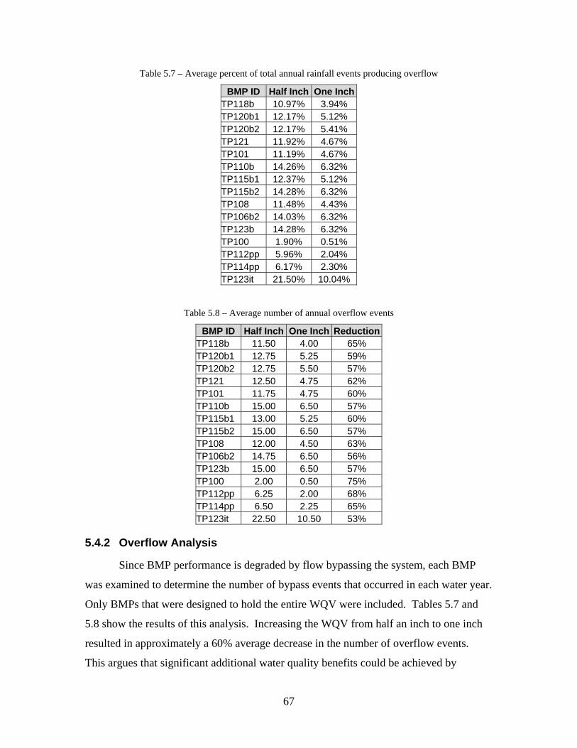
67

Table 5.7 – Average percent of total annual rainfall events producing overflow

BMP ID Half Inch One InchTP118b 10.97% 3.94% TP120b1 12.17% 5.12% TP120b2 12.17% 5.41% TP121 11.92% 4.67% TP101 11.19% 4.67% TP110b 14.26% 6.32% TP115b1 12.37% 5.12% TP115b2 14.28% 6.32% TP108 11.48% 4.43% TP106b2 14.03% 6.32% TP123b 14.28% 6.32% TP100 1.90% 0.51% TP112pp 5.96% 2.04% TP114pp 6.17% 2.30% TP123it 21.50% 10.04%

Table 5.8 – Average number of annual overflow events

BMP ID Half Inch One Inch ReductionTP118b 11.50 4.00 65% TP120b1 12.75 5.25 59% TP120b2 12.75 5.50 57% TP121 12.50 4.75 62% TP101 11.75 4.75 60% TP110b 15.00 6.50 57% TP115b1 13.00 5.25 60% TP115b2 15.00 6.50 57% TP108 12.00 4.50 63% TP106b2 14.75 6.50 56% TP123b 15.00 6.50 57% TP100 2.00 0.50 75% TP112pp 6.25 2.00 68% TP114pp 6.50 2.25 65% TP123it 22.50 10.50 53%

5.4.2 Overflow Analysis

Since BMP performance is degraded by flow bypassing the system, each BMP

was examined to determine the number of bypass events that occurred in each water year.

Only BMPs that were designed to hold the entire WQV were included. Tables 5.7 and

5.8 show the results of this analysis. Increasing the WQV from half an inch to one inch

resulted in approximately a 60% average decrease in the number of overflow events.

This argues that significant additional water quality benefits could be achieved by

68

moving to the more stringent WQV requirements. However, this reduction could be

misleading. Table 5.12 demonstrates that even with the half-inch WQV, most of the

BMPs only experienced overflow during 10-15% of the rainfall events. This indicates

that even at the lower treatment level, the BMPs still fully treat on average 85-90% of the

total annual events. Although the one-inch WQV clearly outperforms the half-inch

WQV, depending on the treatment goals the half-inch WQV may be sufficient and would

likely result in significant installation cost savings over the one-inch WQV.

5.4.3 Drainage Area / Surface Area Ratio Analysis

One consistent result is that the porous pavement BMPs produced significantly

higher removal rates than the bioretention BMPs. In the original Treatment Node and

Infiltration models, this could be explained by the fact that the porous pavement BMPs

were designed to hold the 2-year storm event, not just the normal ½ inch WQV. But in

the Half-Inch and One-Inch models, the porous pavement BMPs were resized to hold the

same WQV as the other BMPs. Despite this, they still significantly outperformed the

other BMPS. This behavior was linked to a general trend in the ratio of the surface area

of a BMP to its drainage area. Figure 5.10 illustrates this trend. All TSS removal rates

presented were averaged across the four simulated water years.

70%

80%

90%

100%

0.00 1.00 2.00 3.00 4.00 5.00 6.00

Drainage Area to Surface Area Ratio

TSS

Rem

oval

(%)

One Inch Half Inch

Figure 5.10 – TSS Removal vs. Drainage Area / Surface Area Ratio

69

In creating this figure, all BMPs that experienced backwater effects or that only

treated part of the incoming flow were omitted. The remaining points show a clear trend

towards decreasing effectiveness with increasing drainage area to surface area ratio,

despite being designed for the same runoff depth. The trend is more pronounced with the

lower WQV in the Half-Inch model. The two highest points correspond to the two

included porous pavement BMPs (TP100 and TP112pp). The one anomalous point near

the end of the series belongs to the bioretention BMP TP118b. This BMP experienced

flooding at the storage node. Since ponding was enabled, this allowed more time for

water to escape through the pump, inflating the treatment percentage. In reality the

excess water would have bypassed the BMP, reducing its effective treatment percentage.

Since the actual BMPs used in the model differ in many minor details such as

slope, shape, etc., a controlled test was conducted. The surface area of a representative

bioretention BMP was kept constant and its drainage area was gradually increased in

order to simulate higher drainage area to surface area ratios. Other than surface area and

basin width, all properties of the drainage area were kept constant. The basin width of

the drainage area was set to the square root of the total area, maintaining a constant

square basin. The Average year was used for simulation. Figure 5.11 illustrates the

results.

y = 0.0054x2 - 0.0794x + 0.9586R2 = 0.9999

60%

70%

80%

90%

100%

0 1 2 3 4 5 6

Drainage Area to Surface Area Ratio

TSS

Rem

oval

(%)

Figure 5.11 – Controlled drainage area / surface area ratio experiment

70

Under these controlled conditions, a quadratic decline can clearly be seen. In

moving from a ratio of 1 to 5, the treatment percentage declined from 88% to 70%. The

same trend applies to the relationship between the treatment percentage and the depth of

the BMP. This is not surprising since by keeping the surface area of the BMP constant

while increasing the contributing area, the depth of the BMP had to increase

proportionally in order to accommodate the increase in water volume. Further testing

showed that the magnitude of the coefficients were very sensitive to the selected WQV

and the surface area of the BMP, but the general quadratic behavior was consistent. The

curve also changes depending on rainfall conditions. The curve presented was based on

the Average year. When simulated using the Wet year, the curve lowered but was still

quadratic. Further research will be necessary to determine if the coefficients can be

determined beforehand in order to create a predictive tool. But the consistent trend

across all variable changes does indicate that as a general design principle, the BMP

drainage area to surface area ratio should be kept as small as possible. These correspond

well with the general bioretention sizing guideline stating that the drainage area to

surface area ratio should not be more than 5:1 (Young and Kibler, 2006).

71

6 Detention Pond Sizing Design storms are commonly used when sizing a detention pond. Regulations

often state a maximum outflow and water surface elevation for a design storm of given

return period and duration. But similar to the behavior observed in the BMP

performances where real rainfall traces often produced conditions that were not ideal and

degraded overall performance, the use of design storms cannot take into account the

variations seen in real life. When properly designed, detention ponds are capable of

providing significant water quality benefits through sedimentation (Loganathan et al.,

1994), but it is questionable whether or not the design storm approach provides the

proper conditions for this to occur.

This chapter examines the effects of long-term simulations on two existing

detention structures in Blacksburg. Their behavior when subjected to one-hour design

storms is compared with the results obtained from the long-term simulations using the

Average and Wet water years.

6.1 Pond Selection

The two ponds selected for testing were the Upper and Lower Francis Lane

ponds, shown in Figure 6.1. These two ponds were used as part of the model verification

in section 3.7. Each pond receives flow from its own hydrologically isolated basin, and

the upper pond discharges into the lower pond. Original design documents gave the

predicted water surface elevations for the 2-, 10- and 100-year one-hour storm events.

The ponds were simulated using the one-hour design storms created in chapter 3. Tables

6.1 and 6.2 show a summary of the predicted pond depths.

72

Figure 6.1 – Location of Francis Lane ponds

Table 6.1 – Pond depths for the Upper Francis Lane pond

Return Pond Depth (ft) Period Design SWMM5 2-year 2.95 3.21

10-year 3.75 4.67 100-year 4.48 6.54

Table 6.2 – Pond depths for the Lower Francis Lane pond

Return Pond Depth (ft) Period Design SWMM5 2-year 2.01 2.57

10-year 3.10 3.86 100-year 4.21 5.06

SWMM5 predicted depths that were higher than the original design estimates.

This could be due to a number of things such as lack of detail on the storage-elevation

curves, differing delineations of the contributing watersheds, or new development in the

watershed since the ponds were constructed. SWMM5’s 100-year simulation for the

73

upper pond was particularly high. Because it was SWMM5 that was also used for the

long-term simulations, the SWMM5 predicted depths were used for comparison.

6.2 Rainfall

All four water years were examined to see which ones contained significant storm

events or generated significant water depths in the ponds. Using NOAA Atlas 14

(NOAA, 2006) as a reference, the individual storm events in each year were identified

and classified according to their return periods. The Small year had no events above a 2-

year return period. The largest storm in the Dry year had a 3-year return period. Neither

year produced any significant depths in the ponds. Because of the lack of large storm

events or significant pond depths, these years were not included in this analysis. The

Average year contained two 10-year storms. All other events fell below the 2-year level.

The Wet year contained a 5-, 25- and 75-year event with all other storms being below the

2-year level. Table 6.3 contains the rainfall data.

Table 6.3 – Large rainfall events in the Average and Wet years

Year Rainfall

(in) Duration

(hrs)

Return Period (years)

Average 3.81 22 10 Average 4.81 35 10

Wet 6.60 30 75 Wet 5.22 36 25 Wet 3.23 22 5

The highest pond depths for both ponds during the Average year corresponded to

the two storm events mentioned in Table 6.3. The highest depths in the Wet year

corresponded to the 25- and 75-year events. The rainfall events were relatively isolated,

with no significant rainfall occurring for some time before them; however, they did often

have several small rain events in the previous five days. There were no instances where a

long period of low-level rainfall resulted in significant pond depths.

74

6.3 Detention Pond Analysis

Graphs of the full yearly depths for the upper and lower ponds can be found in

Appendix F. Figures 6.2 and 6.3 illustrate the pond responses to the largest of the storm

events.

0

1

2

3

4

5

6

7

8

340 340.5 341 341.5 342 342.5 343

Time (Days)

Dep

th (f

t)

0

0.2

0.4

0.6

0.8

1

1.2

1.4

1.6

Rai

nfal

l (in

/hr)

Depth Rainfall

Figure 6.2 – Upper Francis Lane response to 75-year storm event

0

1

2

3

4

5

6

7

8

9

340 340.5 341 341.5 342 342.5 343

Time (days)

Dep

th (f

t)

0

0.2

0.4

0.6

0.8

1

1.2

1.4

1.6

Rai

nfal

l (in

/hr)

Depth Rainfall

Figure 6.3 – Lower Francis Lane response to 75-year storm event

75

During the Average year the upper pond level only crossed the predicted 2-year

depth once and never crossed the predicted 10-year depth, despite experiencing two 10-

year events. The lower pond crossed the predicted 10-year depth for both the 5- and the

10-year events. All other peaks were well below the 2-year depth. During the Wet year,

both the upper and lower ponds vastly exceeded the 100-year depth during the 75-year

storm event. For the upper pond, all other peaks were below the 2-year depth. For the

lower pond the 25-year storm exceeded the 10-year depth as expected, but no other

storms crossed the 2-year depth.

One possible reason why many of the real storms generated lower than expected

pond depths is that different systems were used to create the original design storms and to

classify the events in the long-term simulations. The original 1-hour design storms were

created from the Montgomery County IDF charts using VTPSUHM. The rainfall events

in the long-term simulations were classified using NOAA Atlas14 (NOAA, 2006). These

two systems disagree on the rainfall totals for 1-hour storm events. Table 6.4 illustrates.

Table 6.4 – Rainfall depths for 1-hour design storms

(in inches)

Return Period

Mont. IDF

NOAA Atlas 14

2 1.56 1.23 10 2.30 1.80

100 3.21 1.89

As can be seen, Atlas 14 consistently gives lower rainfall depth values than the

IDF charts for the same return periods. Storms classified using Atlas 14 would have a

higher return frequency if they had been classified using the IDF charts, thus explaining

why many of the 5-year events (as classified by Atlas 14) produced depths below the

predicted 2-year depths (as classified using the IDF charts). The IDF charts were not

used for all events because they do not include storm events above one hour in duration.

The differing classifications do not explain why a storm classified as a 75-year

event using Atlas 14 exceeded the 100-year depth as determined by the IDF charts.

During this event both ponds actually failed, exceeding their maximum design depth.

Because the ponding option was enabled in SWMM5, the floodwaters were maintained at

76

the ponds as additional depth above the maximums. Since this was the only event that

significantly exceeded the design storm predictions, it was examined in more detail.

The following discussion focuses on the subcatchment for the upper pond only,

although the ideas are applicable to both ponds. The 100-year design storm produced

3.21 inches of rainfall in one hour. At the beginning of the design storm, the soil was

completely dry, and none of the initial depression storage had been met. This resulted in

a runoff coefficient of 0.436 and 110328 ft3 of runoff. The 75-year event during the Wet

year produced 6.6 inches over 30 hours. The initial low-intensity rainfall occurring over

several hours as well as the minor rainfall from the previous day combined to saturate the

soil and fill the depression storage before the peak of the storm arrived. The result was a

much higher runoff coefficient of 0.784 and a much higher runoff volume of 408340 ft3.

Even when modeled as a stand-alone event, thus removing the previous day’s rainfall, the

storm produced a runoff coefficient of 0.686 and still caused the pond to fail. Table 6.5

shows the runoff coefficients for the 100-year design storm, the 75-year event, and the

75-year event as a standalone (SA) storm for both the upper and lower ponds.

Table 6.5 – Runoff coefficients

Q100 Q75 Q75 SA Upper 0.436 0.785 0.686 Lower 0.472 0.803 0.711

To check whether or not new storm events occurred while the ponds were still

draining from previous events, SWMM5 was used to calculate the inter-event times for

the basin runoff events, pond empty times and pond outflows across all four water years.

The results are shown in Table 6.6. Table 6.6a shows the inter-event times for the runoff

from the subcatchments contributing to the two ponds. Table 6.6b shows the time

between when there is water in the ponds, representing the times when the ponds are

empty. Table 6.6c shows the inter-event times at the outflows of each pond. The last

row, “Lower OF,” depicts the overflow conduit for the lower pond. The final column in

all three tables represents the total number of events (and subsequent inter-events) that

were seen.

77

Table 6.6 – Inter-event times for the Upper and Lower Francis Lane ponds

Inter-event runoff time (hours) Total Basin Max Min Avg Events Upper 563.5 6 84.38 369 Lower 563.5 6 86.62 356

(a)

Inter-event volume (hours) Total

Pond Max Min Avg Events Upper 533 6 86.88 216 Lower 557 6 88.49 280

(b)

Inter-event outflow (hours) Total

Pond Max Min Avg Events Upper 515 6 84.76 178 Lower 515 6 85.84 174

Lower OF 4888.5 3451 4360.67 3 (c)

The average dry periods for the two ponds were slightly longer than the average

time between runoff events, indicating that the ponds were usually dry before the next

event arrived. However, there were far fewer volume events than runoff events, meaning

that at times a single water volume event in the ponds had to span multiple runoff events.

This indicates that a number of runoff events occurred at times when the ponds were not

completely empty from the previous event, thus reducing the effective detention capacity

of the ponds. This has great potential to cause the ponds to fail, although no instance of a

failure due to these circumstances was seen in the modeled years.

The results presented here clearly show that the design storm approach is not

capable of covering all possible rainfall conditions. The inter-event analysis indicates

that the ponds often receive runoff from new events before the volume from the previous

events has been completely removed. The 75-year storm event shows that longer rainfall

events can saturate the soil before the peak of the storm, resulting in pond failures even

when the ponds were technically designed to handle the event. However, figures F.1

through F.4 in Appendix F indicate that the ponds can normally handle the flows entering

them and often have significantly lower peak depths than expected. It is only under

extreme circumstances that these ponds failed. This indicates that the design storm

approach does provide a valid starting point for sizing ponds. Further research involving

78

more sample detention ponds and more years of rainfall would need to be conducted in

order to draw any definitive conclusions.

79

7 Conclusions and Recommendations

7.1 Restatement of Objectives

This research had several objectives. A primary objective was to test SWMM5’s

ability to model BMPs. In pursuance of this, a city stormwater model was created using

SWMM5. Multiple BMP retrofits were identified throughout the town and placed within

this model. Multiple methods were used to model the BMPs. The model was then

subjected to both design storms and continuous hourly rainfall traces. The performance

of the BMPs, as well as that of SWMM5 itself, was then compared across all simulations

and to the expected results. The appropriateness of the half-inch water quality volume

was tested and compared against the benefits of increasing to a one-inch water quality

volume. The short- and long-term simulations were also used to test the appropriateness

of using design storms when sizing a detention basin.

7.2 The Duck Pond Watershed Model

The SWMM5 model produced in this research was the first model to include

detailed information about the entire Duck Pond watershed. Previous attempts have

modeled only small sections of the system, usually stopping at the town/campus

boundary (Tremel, 1998), or they have modeled a much larger area in much less detail,

reducing the Duck Pond watershed into just a few large subcatchments with lumped

parameters and no infrastructure detail (Thye, 2003; BSE, 2003). To create the model,

sources had to be used that contained significant deficiencies. This resulted in a final

model where parts of the system were based on good, reliable data while others were

based on best-guess approximations. Detailed validation of the model was not possible

because of a lack of gauging stations within the watershed. Isolated portions of the

model were compared to the small amount of data available, producing reasonable

results.

In order to improve the accuracy of the model, two things are necessary. First, a

detailed survey of the town’s stormwater system must be conducted. This has been done

in the past, but vital information such as inverts was omitted. Information on open-

channel flows and detention ponds also needs to be collected. The estimates used to

80

construct the model need to be replaced with hard data. Secondly, in order to fully

validate this model or any future models, flow rate and quality monitoring stations need

to be installed throughout Blacksburg and on the Virginia Tech campus. In order to

achieve a reasonable level of detail so that problem areas can be identified, monitoring

stations would need to be set up at multiple points throughout the watershed, not just at

its outlet. Efforts have been made to establish some such monitoring points on campus,

but to date these have not been completed.

7.3 BMP Modeling with SWMM5

SWMM5 is quite good at modeling stormwater flows through the various

elements of a model; however, in its current form it is limited in its ability to model

pollutant transport and the treatment aspects of BMPs. SWMM5 has a number of built-in

features design to model BMPs. Most are useful at a small scale, when the

subcatchments can be discretized to the point where each land cover type is broken out

into its own subcatchment. At larger scales where such minute discretization is not

possible or at least not feasible, many of these features break down to the point where

they are no longer useful at all. SWMM5’s lack of ability to infiltrate from nodes or

conduits forces the modeler to resort to awkward surrogates that lack the ability to

properly account for all aspects of infiltration. The inability to accurately model short-

circuiting within a BMP also requires the use of elaborate configurations to properly

separate incoming flows before treatment. Such arrangements introduce instabilities to

the system that otherwise would not exist. Finally, continuity issues can arise when

routing pollutant mass, resulting in significant mass being created as the flow progresses.

Several features could be added to SWMM5 that would greatly improve its

BMP modeling ability. Primary among these would be the ability to infiltrate from

conduits and nodes, and the ability to achieve quality improvements during pipe flow.

The later was a feature in earlier versions of SWMM, and it is hoped that it will be added

back in future releases. Another significant feature enhancement would be the ability to

specify a short-circuit path, allowing the modeler to specify that all flows above a certain

level will not receive treatment. The most recent version of SWMM5 (5.0.008) provided

significant improvements in quality routing continuity; however, some issues still persist

81

and need to be addressed in future releases. Finally, if SWMM5 is to become a true BMP

modeling platform it needs to have the ability to go beyond just the treatment function

and be able to model actual fundamental treatment processes such as those suggested by

Lai et al. (2005) and Huber et al. (2005a).

7.3 BMP Performance

Despite SWMM5’s deficiencies, it was still possible to create a stormwater model

that incorporated local BMPs into a large-scale watershed model. Although the specific

numbers associated with the models are somewhat suspect due to continuity issues, many

overall trends were discernable. Primarily, impact due to the local BMPs was seen at the

system level, albeit only on the order of 1 to 3%. Relatively little of the overall drainage

area received any treatment at all, and the BMPs that were used were sited based on

current land use and land availability, not according to any optimal placement strategy.

Given these limiting factors, it is very encouraging that any system-wide results were

discernable. It also suggests that if a concerted effort was made to place larger numbers

of BMPs in a watershed in critical locations, more significant impacts could be achieved.

Most of the modeled BMPs performed well. At the local level they generally

achieved treatment percentages that were near theoretical expectations; however, these

locally high treatment levels were quickly diminished as the treated flows mixed with

other untreated flows when moving downstream. A strong correlation was seen between

the volume of flow treated by the BMPs and the amount of treatment seen at the

watershed level. It was hoped that a trend could be established between the percentage of

surface area treated and the treatment seen at the system level, but this was not the case.

With some BMPs only treating a partial WQV, obtaining a meaningful account of

drainage area treated became impossible. Even when these were removed from the

system, the results showed no discernable pattern.

A very interesting result was the relationship seen between the ratio of the

drainage area to the BMP surface area. Under controlled conditions with a single type of

BMP, treatment decreased according to a quadratic function as the ratio increased. This

implies a general design principle that the drainage area to BMP surface area ratio should

82

be kept as small as possible in order to maximize the BMP’s performance. This principle

was not limited by the actual size of the BMP.

Testing of the half-inch rule for determining WQV yielded interesting results. In

general, the BMPs designed to hold exactly half an inch of runoff achieved close to or

exceeded the predicted values. BMP overflow only occurred in 10-15% of rainfall

events. These results were obtained using the minimum 0.5 in/hr infiltration rate and

assuming a constant pollutant inflow concentration. With any increase in infiltration rate

or with the presence of even minor first-flush behavior, these results indicate that the

expected treatment rates could be achieved. This validates the half-inch principle, at least

for this area and under the assumed conditions. As expected, increasing to a one-inch

WQV increased the performance even further.

An exception to this standard half-inch rule occurred when the drainage area

contained a significant amount of pervious land cover. According to VDOT regulations

(VDOT, 2004), the half-inch rule is only applied to the impervious fraction of the

catchment, which assumes that only the impervious portion of the catchment contributes

significantly to the runoff. In cases where the pervious fraction is significant, this

assumption proved to be false. The pervious runoff easily overwhelmed the BMP,

resulting in a significant degradation of its performance.

7.4 Design Storms and Continuous Simulation

The comparison of design storms versus continuous simulations for the sizing of

detention ponds provided clear indications that the design storm approach alone is not

sufficient. The design storm approach failed to account for long, slow events that

saturated the ground. Many instances were also seen where the detention ponds were not

completely empty before a new storm event arrived. If the purpose of a new pond is to

prevent all overflow, continuous modeling is necessary. Even when limiting overflow

events is not the primary concern, the design storm approach should be backed up with

continuous modeling in order to help predict the expected number of overflow events.

Despite these cautions, the ponds examined were able to function effectively under

almost all of the circumstances experienced during the continuous simulation. Given the

limited scope of this experiment, it is difficult to draw any definitive conclusions;

83

however, it does appear that the design storm approach does provide at least a reasonable

starting point for detention pond sizing.

84

References Brown, A. and Huber, W. C. (2004). “Hydrologic Characteristics Simulation for BMP Performance Evaluation.” ASCE-EWRI World Water and Environmental Resources Congress. Salt Lake City, Utah. “Calculations: Virginia Polytechnique Institute and State University Alumni/CEC/Hotel Complex.” H&A Consulting Engineers, Project Number R3832.00. September 16, 2002. Revised March 10, 2003. Chow, V. T. (1959). Open Channel Hydraulics, McGraw-Hill, New York. Creggar, W. H., Hudson, H. C. and Porter, H. C. (1985). Soil Survey of Montgomery County, Virginia. Soil Conservation Service, U. S. Department of Agriculture, Washington, D. C. Department of Biological Systems Engineering (BSE), Virginia Tech (2003). “Benthic TMDL for Stroubles Creek in Montgomery County, Virginia.” Prepared for Virginia Department of Environmental Quality and Virginia Department of Conservation and Recreation, Richmond, VA. Engman, E. T. (1986). “Roughness Coefficients for Routing Surface Runoff.” Journal of Irrigation and Drainage Engineering, ASCE, 112(1), pp. 39-53. GISDataDepot (2006). “Free GIS Data – GIS Data Depot.” http://data.geocomm.com/. Accessed August 13, 2006. Hayes, Seay, Mattern and Mattern, Inc. (HSMM). (1994). Stroubles Creek Stormwater System. Prepared for Town of Blacksburg, Virginia. November 1994. Huber, W. C. and Cannon, L. (2002). “Modeling Non-Directly Connected Impervious Areas in Dense Neighborhoods.” ASCE Conference Proceedings 112(21). Huber, W. C., Lai, F., Cannon, L., and Stouder, M. (2005a). “Modeling Concepts for BMP/LID Simulation.” ASCE-EWRI World Water and Environmental Congress. Anchorage, Alaska. Huber, W. C., Wells, W. J., and Besaw, I. K. (2005b). “Application of SWMM5 for BMP/LID Quality Evaluation.” ASCE-EWRI World Water and Environmental Congress. Anchorage, Alaska. International Stormwater Best Management Practices Database. http://www.bmpdatabase.org/. Accessed August 13, 2006.

85

Jones, J. E., Langan, T., Fassman, E. A., Urbonas, B., Strecker, E., Quigley, M. (2004). “Why Is It so Difficult to Acquire Reliable BMP Performance Data?” ASCE-EWRI World Water and Environmental Resources Congress. Salt Lake City, Utah. Lai, F., Shoemaker, L., and Riverson, J. (2005). “Framework Design for BMP Placement in Urban Watersheds.” ASCE-EWRI World Water and Environmental Congress. Anchorage, Alaska. Latham, M. J. (1996). “An Assessment of Models and Methodologies Used in the Design of Detention Facilities for Small Urban Watersheds.” MS Thesis, Virginia Polytechnic Institute and State University, at Blacksburg, VA. Loganathan, G. V., Watkins, E. W., and Kibler, D. F. (1994). “Sizing Storm-Water Detention Basins for Pollutant Removal.” Journal of Environmental Engineering, ASCE, 120(6), pp. 1380-1399. MaSTEP Stormwater Technologies Clearinghouse (2004). University of Massachussets. Amerhest, MA. http://www.mastep.net/. Accessed August 13, 2006. McGuiness, J. L. and Bordne, E. F. (1972). “A Comparison of Lysimeter Derived PET With Computed Values.” ARS, USDA Technical Bulletin 1452. NOAA (2006). “National Weather Service – HDSC Precipitation Frequency Data Server.” http://hdsc.nws.noaa.gov/hdsc/pfds/. Accessed August 13, 2006. Palmer, V. J. (1946). “Retardance Coefficients for Low Flow in Channels Lined with Vegetation.” Transactions of the American Geophysical Union, 27(11), pp. 187-197. Pennsylvania Department of Environmental Protection (PADEP) (2005). Draft Stormwater Best Management Practices Manual. Quigley, M. M., Streker, E. W., Leisenring, M., Huber, W. C., Heaney, J., Weinstein, N., Sansalone, J., and Bodine, D. (2005). “The Integrated Unit Process Design Approach for Urban Water Quality Design.” ASCE-EWRI World Water and Environmental Congress. Anchorage, Alaska. Sansalone, J. J. and Cristina, C. M. (2004). “First Flush Concepts for Suspended and Dissolved Solids in Small Impervious Watersheds.” Journal of Environmental Engineering, ASCE, 130(11), pp. 1301-1314. Thye, F. B. (2003). “Virginia Tech Duck Pond Retrofit for Improved Water Quality in Stroubles Creek.” MS Project, Virginia Polytechnic Institute and State University, at Blacksburg, VA. Blacksburg, Town of. “Welcome to the Blacksburg GIS Data Distribution Site.” Blacksburg, VA. http://gis-server.lib.vt.edu/blacksburg/. Accessed August 13, 2006.

86

Tremel, M. (1998). “Stormwater Management Pond Study for Donaldson Brown on Virginia Tech Campus.” Town of Blacksburg. Blacksburg, Virginia. U.S. Department of Agriculture (USDA) Soil Conservation Service (1986). “Urban Hydrology for Small Watersheds.” Technical Release No. 55. Washington D.C. Virginia Department of Transportation (VDOT). (2004). VDOT Erosion and Sediment Control and Stormwater Management Program Manual. Woolhiser, D. A., Smith, R. E., and Goodrich, D. C. (1990). “KINEROS, A Kinematic Runoff and Erosion Model: Documentation and User Manual.” U.S. Department of Agricultural Research Service, ARS-77, Tucson, AZ. Young, K. D. and Kibler, D. F.(2006). Lehigh Valley Planning Commission BMP Design Manual of Practice. Prepared for the Lehigh Valley Planning Commission.

87

Appendix A Acronyms

88

ArcGIS GIS software package produced by ESRI

ASC ArcGIS-to-SWMM-Converter; used to generate SWMM5 files from a GIS

database

BMP Best Management Practice

CGIT Center for Geospatial Information Technology, Virginia Tech

DEM Digital Elevation Map

EMC Event Mean Concentration

EPA SWMM Environmental Protection Agency Storm Water Management Model

GIS Geographical Information System

HSG Hydrologic Soil Group

HSMM Hayes, Seay, Mattern and Mattern, Inc.

IDF Intensity-Duration-Frequency

NOAA National Oceanic and Atmospheric Administration

PP Porous Pavement

S&ID Site and Infrastructure Development department, Virginia Tech

SCS Soil Conservation Service

SWMM EPA SWMM

SWMM4 EPA SWMM 4

SWMM5 EPA SWMM 5

TMDL Total Maximum Daily Load

TSS Total Suspended Solids

VTPSUHM Virginia Tech & Penn State Urban Hydrology Model

WQI Water Quality Inlet

WQO Water Quality Orifice

WQV Water Quality Volume

89

Appendix B Programs and Macros

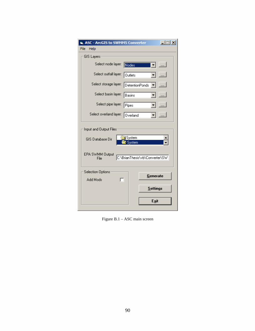
90

Figure B.1 – ASC main screen

91

Figure B.2 – Set Fields screen in ASC

Figure B.3 – SWMM system options screen in ASC

92

Figure B.4 – CN Calculator Macro for ArcGIS

93

Appendix C Modeling Data

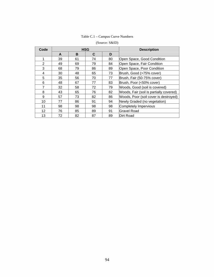
94

Table C.1 – Campus Curve Numbers

(Source: S&ID)

Code HSG Description A B C D 1 39 61 74 80 Open Space, Good Condition 2 49 69 79 84 Open Space, Fair Condition 3 68 79 86 89 Open Space, Poor Condition 4 30 48 65 73 Brush, Good (>75% cover) 5 35 56 70 77 Brush, Fair (50-75% cover) 6 48 67 77 83 Brush, Poor (<50% cover) 7 32 58 72 79 Woods, Good (soil is covered) 8 43 65 76 82 Woods, Fair (soil is partially covered) 9 57 73 82 86 Woods, Poor (soil cover is destroyed)

10 77 86 91 94 Newly Graded (no vegetation) 11 98 98 98 98 Completely Impervious 12 76 85 89 91 Gravel Road 13 72 82 87 89 Dirt Road

95

Table C.2 – Town Curve Numbers, Adjusted

(Unadjusted Source: USDA,1986)

Code HSG Description A B C D

A 49 69 79 84 Agricultural - Pasture, No Mech. Treat., Fair

C 38 58 71 78 Commercial (85% Avg Imperv)

CND 38 61 75 81 Condos - Row Houses (65% Avg Imperv, <1/8 Acre lots)

CV 68 79 86 89 Civic - Poor Condition, grass cover < 50%

CV-CEM 36 61 74 80 Civic/Cemetary - Good Condition, grass cover > 75%

CV-SH 38 61 74 80 Civic/Special Housing, Greeks - 1/4 ac Res (38% avg imperv)

DP 38 61 74 80 Duplex - 1/4 ac Res (38% avg imperv)

LD 39 61 74 80 Low-Density Residential/Ag - 2 ac Res (12% avg imperv)

MFC 38 61 74 80 Multi-Family Complex - 1/4 ac Res (38% avg imperv)

MH 38 61 74 80 Mobile Homes - 1/4 ac Res (38% avg imperv)

MXCO 38 58 71 78 Mixed Use Comm/Office - Comm&Bus areas (85% avg imperv)

MXCR 38 58 71 78 Mixed Use Comm/Res - Comm&Bus areas (85% avg imperv)

MXOR 39 61 74 81 Mixed Use Office/Res - 1/3 ac Res (30% avg imperv)

MXCOR 38 58 71 78 Mixed Use Comm/Off/Res - Comm&Bus areas (85% avg imperv)

O 38 61 75 81 Professional Offices - 1/8 ac (65% avg imperv)

P 39 61 74 80 Parks & Trails - Parks, Good condition (grass cover > 75%)

R 98 98 98 98 Road, building or other impervious surface

RD 37 62 73 80 Light Industry R&D - Industrial Districts (72% avg imperv)

ROW 68 79 86 89 Right of Way - Open spaces, poor condition

SF 38 61 74 80 Single Family - 1/4 ac Res (38% avg imperv)

TH 38 61 75 81 Town Homes - 1/8 ac Town houses (65% avg imperv)

U 38 61 75 81 University - 1/8 ac Res (65% avg imperv)

V 39 61 74 80 Vacant - Parks, Good condition (grass cover > 75%)

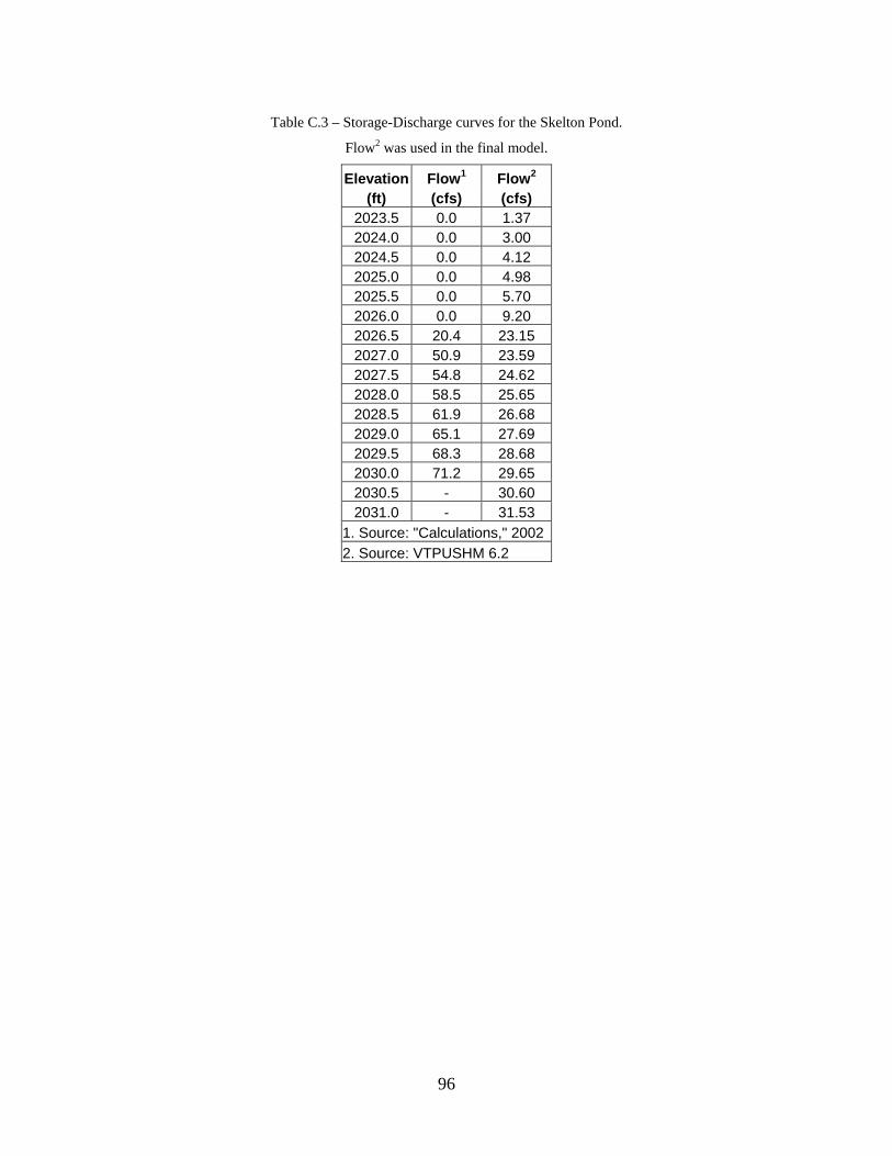
96

Table C.3 – Storage-Discharge curves for the Skelton Pond.

Flow2 was used in the final model.

Elevation Flow1 Flow2 (ft) (cfs) (cfs)

2023.5 0.0 1.37 2024.0 0.0 3.00 2024.5 0.0 4.12 2025.0 0.0 4.98 2025.5 0.0 5.70 2026.0 0.0 9.20 2026.5 20.4 23.15 2027.0 50.9 23.59 2027.5 54.8 24.62 2028.0 58.5 25.65 2028.5 61.9 26.68 2029.0 65.1 27.69 2029.5 68.3 28.68 2030.0 71.2 29.65 2030.5 - 30.60 2031.0 - 31.53

1. Source: "Calculations," 20022. Source: VTPUSHM 6.2

97

Appendix D BMP Design Data

98

Table D.1 – Overview of BMPs included in the model

Name BMP Area

Contributing Area

Impervious Fraction WQVTot

(1) WQVTreated BMP Soil Group (ac) (ac) % ft3 ft3

TP100(2) 0.242 0.484 100.00% 4850 4850 PP 12C/12B/16BTP101 0.383 1.579 100.00% 2866 2866 Bioretention 33/11B/16C TP104(3) 0.979 48.955 16.78% 14909 14909 Wetlands 18B/18C TP106b2 0.034 0.171 100.00% 310 310 Bioretention 18B TP106r 0.300 0.300 100.00% 545 545 Vegetated Roof 18B TP107(2) 0.849 36.736 2.46% 368050 6041 Infiltration Basin 18B/18C/18DTP108 0.083 0.316 100.00% 573 573 Bioretention 18B TP109 0.079 27.679 23.52% 11816 1182 Grassy Swale 29/18B TP110 0.235 0.235 100.00% 427 427 Vegetated Roof 29 TP112(2) 0.146 0.393 100.00% 3940 3940 PP 29 TP114pp(2) 0.300 0.867 100.00% 8685 8685 PP 29 TP115b1 0.029 0.125 100.00% 227 227 Bioretention 29 TP115b2 0.046 0.256 100.00% 464 464 Bioretention 29 TP118(3) 0.196 0.978 100.00% 1776 1776 Bioretention 18B/13C TP118 0.394 0.394 100.00% 716 716 Vegetated Roof 18B/13C TP118(5) 0.089 5.803 17.53% 1846 1846 Infiltration Basin 18B/13C TP120b1 0.080 0.322 100.00% 585 585 Bioretention 16B/18B TP120b2 0.092 0.399 100.00% 724 724 Bioretention 16B/18B TP121 0.130 0.515 100.00% 935 935 Bioretention 16C/16B TP123it 0.062 3.665 20.66% 1374 1374 Infiltration Trench 29/18C/18B TP123b(3) 0.027 0.134 100.00% 243 243 Bioretention 29/18C/18B (1) Unless otherwise noted, WQV is computed as 1/2 inch over the entire impervious area, as per VDOT regulations. (2) This WQV was computed based on the full 2-year, 1-hour design depth of 1.563 inches. (3) This BMP could not handle the entire drainage area, so only the percentage routed to the BMP is listed.(4) This is the sum of three separate bioretention BMPs on the same site. (5) This assumes that the other BMPs on this site (bioretention and vegetated roof) are already installed and functioning.

99

Figure D.1a – Map of BMP locations

100

Figure D.1b – Map of BMP locations

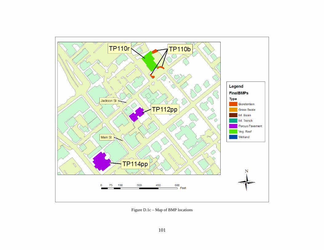
101

Figure D.1c – Map of BMP locations

102

Figure D.1d – Map of BMP locations

103

Appendix E BMP Simulation Results

104

E.1 One-Hour Design Storms

Table E.1 – TSS removal for Treatment Node model

TSS Removal 1/2 Inch 1 Inch Q2

System 1.30% 0.63% 0.23% North

Branch 1.25% 1.03% 0.66% South

Branch 3.54% 2.65% 1.58%

Table E.2 – Volume reduction for Treatment Node model

Volume Reduction 1/2 Inch 1 Inch Q2

System 0.07% 0.06% 0.04% North

Branch 0.03% 0.04% 0.00% South

Branch 0.00% 0.18% -0.04%

Table E.3 – Percent of volume treated by Treatment Node model

Percent Volume Treated 1/2 Inch 1 Inch Q2

System 4.07% 2.66% 1.77% North

Branch 1.88% 1.47% 1.05% South

Branch 6.83% 4.22% 2.70%

105

Table E.4 – TSS removal for Infiltration model

TSS Removal 1/2 Inch 1 Inch Q2

System 3.14% 2.23% 1.35% North

Branch 1.37% 1.24% 0.79% South

Branch 3.90% 3.12% 1.88%

Table E.5 – Volume reduction for Infiltration model

Volume Reduction 1/2 Inch 1 Inch Q2

System 1.52% 1.41% 1.03% North

Branch 1.42% 1.24% 0.85% South

Branch 1.84% 2.11% 1.37%

Table E.6 – Percent of volume treated by Infiltration model

Percent Volume Treated 1/2 Inch 1 Inch Q2

System 1.41% 1.24% 0.88% North

Branch 1.41% 1.24% 0.88% South

Branch 6.76% 4.12% 2.67%

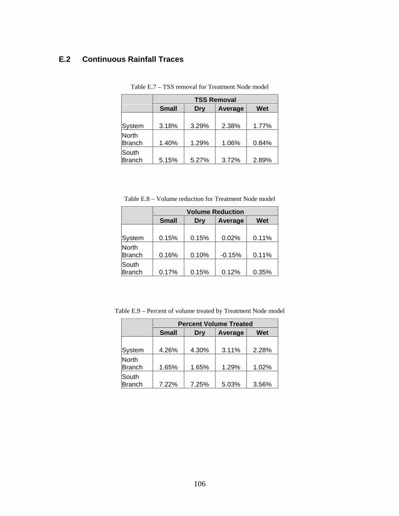
106

E.2 Continuous Rainfall Traces

Table E.7 – TSS removal for Treatment Node model

TSS Removal Small Dry Average Wet

System 3.18% 3.29% 2.38% 1.77% North Branch 1.40% 1.29% 1.06% 0.84% South Branch 5.15% 5.27% 3.72% 2.89%

Table E.8 – Volume reduction for Treatment Node model

Volume Reduction Small Dry Average Wet

System 0.15% 0.15% 0.02% 0.11% North Branch 0.16% 0.10% -0.15% 0.11% South Branch 0.17% 0.15% 0.12% 0.35%

Table E.9 – Percent of volume treated by Treatment Node model

Percent Volume Treated Small Dry Average Wet

System 4.26% 4.30% 3.11% 2.28% North Branch 1.65% 1.65% 1.29% 1.02% South Branch 7.22% 7.25% 5.03% 3.56%

107

Table E.10 – Individual BMP treatment percentages for Treatment Node Model

BMP Treatment Efficiencies Avg BMP ID Small Dry Average Wet Type

TP118b 85.05% 82.73% 78.58% 71.54% 75.06% Bioretention TP120b1 85.17% 82.90% 80.15% 74.31% 77.23% Bioretention TP120b2 85.08% 82.96% 79.01% 73.36% 76.19% Bioretention TP121 85.11% 83.46% 80.42% 75.12% 77.77% Bioretention TP101 67.73% 63.85% 66.55% 9.02% 37.79% Bioretention TP110b 83.93% 81.87% 77.35% 3.89% 40.62% Bioretention TP115b1 85.00% 83.08% 79.73% 74.12% 76.92% Bioretention TP115b2 83.58% 81.67% 76.51% 68.21% 72.36% Bioretention TP108 85.11% 83.72% 80.83% 75.80% 78.32% Bioretention TP106b2 84.20% 81.69% 77.11% 68.49% 72.80% Bioretention TP123b 84.51% 82.07% 77.68% 70.65% 74.17% Bioretention TP100 85.05% 85.11% 83.79% 79.09% 81.44% Porous Pavement TP112pp 84.93% 84.91% 82.79% 77.53% 80.16% Porous Pavement TP114pp 84.88% 84.86% 82.58% -11.23% 35.68% Porous Pavement TP123it 68.17% 65.39% 45.63% 33.02% 39.33% Infiltration Trench TP118inf 44.60% 46.61% 28.10% 18.90% 23.50% Infiltration Basin TP107 51.50% 36.27% 19.96% 11.45% 15.71% Infiltration Basin TP104 26.48% 29.47% 22.39% 14.94% 18.67% Wetland TP109 24.04% 24.36% 14.89% 9.57% 12.23% Grass Swale

108

Table E.11 – Individual BMP inflow treated percentages for Treatment Node model

BMP Percent of Inflow Treated Avg BMP ID Small Dry Average Wet Type

TP118b 98.84% 96.32% 91.99% 84.07% 88.03% Bioretention TP120b1 99.86% 98.81% 98.84% 87.61% 93.22% Bioretention TP120b2 101.77% 101.75% 96.22% 87.69% 91.96% Bioretention TP121 99.24% 97.53% 93.57% 87.53% 90.55% Bioretention TP101 125.95% 127.00% 112.39% 99.92% 106.16% Bioretention TP110b 98.26% 95.51% 90.44% 80.82% 85.63% Bioretention TP115b1 100.57% 98.64% 94.34% 87.50% 90.92% Bioretention TP115b2 97.15% 94.43% 88.98% 79.72% 84.35% Bioretention TP108 99.65% 98.14% 94.56% 88.70% 91.63% Bioretention TP106b2 102.31% 103.55% 94.25% 83.94% 89.09% Bioretention TP123b 101.02% 99.58% 92.87% 84.49% 88.68% Bioretention TP100 97.76% 97.50% 96.54% 91.36% 93.95% Porous Pavement TP112pp 97.94% 97.42% 95.27% 89.50% 92.39% Porous Pavement TP114pp 97.76% 97.32% 95.25% 90.02% 92.64% Porous Pavement TP123it 74.87% 71.78% 49.17% 36.02% 42.59% Infiltration Trench TP118inf 59.66% 62.69% 35.88% 30.92% 33.40% Infiltration Basin TP107 58.15% 40.37% 21.85% 11.95% 16.90% Infiltration Basin TP104 52.79% 57.97% 41.98% 33.88% 37.93% Wetland TP109 33.10% 34.81% 20.63% 13.26% 16.95% Grass Swale TP110r 0.61% 0.58% 0.48% 0.39% 0.44% Veg. Roof TP106r 6.97% 6.71% 5.37% 4.33% 4.85% Veg. Roof TP118r 22.73% 22.07% 16.42% 12.80% 14.61% Veg. Roof

109

Table E.12 – TSS removal for Infiltration model

TSS Removal Small Dry Average Wet

System 3.32% 3.37% 2.50% 1.80% North Branch 1.46% 1.31% 1.12% 0.85% South Branch 5.39% 5.46% 3.95% 3.08%

Table E.13 – Volume reduction for Infiltration model

Volume Reduction Small Dry Average Wet

System 1.52% 1.43% 1.43% 0.89% North Branch 1.43% 1.33% 1.08% 0.84% South Branch 1.91% 1.74% 1.49% 1.43%

Table E.14 – Percent of volume treated by Infiltration model

Percent Volume Treated Small Dry Average Wet

System 4.05% 4.05% 2.96% 2.16% North Branch 1.29% 1.24% 1.00% 0.79% South Branch 7.08% 7.08% 4.96% 3.50%

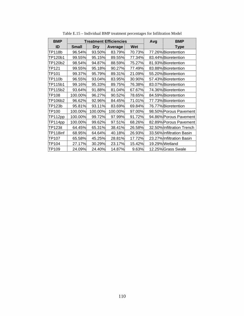
110

Table E.15 – Individual BMP treatment percentages for Infiltration Model

BMP Treatment Efficiencies Avg BMP ID Small Dry Average Wet Type

TP118b 96.54% 93.50% 83.79% 70.73% 77.26% Bioretention TP120b1 99.55% 95.15% 89.55% 77.34% 83.44% Bioretention TP120b2 98.54% 94.87% 88.59% 75.27% 81.93% Bioretention TP121 99.55% 95.18% 90.27% 77.49% 83.88% Bioretention TP101 99.37% 95.79% 89.31% 21.09% 55.20% Bioretention TP110b 96.55% 93.04% 83.95% 30.90% 57.43% Bioretention TP115b1 99.16% 95.33% 89.75% 76.38% 83.07% Bioretention TP115b2 93.64% 91.88% 81.04% 67.67% 74.36% Bioretention TP108 100.00% 96.27% 90.52% 78.65% 84.59% Bioretention TP106b2 96.62% 92.96% 84.45% 71.01% 77.73% Bioretention TP123b 95.81% 93.11% 83.69% 69.84% 76.77% Bioretention TP100 100.00% 100.00% 100.00% 97.00% 98.50% Porous Pavement TP112pp 100.00% 99.72% 97.99% 91.72% 94.86% Porous Pavement TP114pp 100.00% 99.62% 97.51% 68.26% 82.89% Porous Pavement TP123it 64.45% 65.31% 38.41% 26.58% 32.50% Infiltration Trench TP118inf 68.95% 64.64% 40.18% 26.93% 33.56% Infiltration Basin TP107 65.58% 45.25% 28.81% 17.72% 23.27% Infiltration Basin TP104 27.17% 30.29% 23.17% 15.42% 19.29% Wetland TP109 24.09% 24.40% 14.87% 9.63% 12.25% Grass Swale

111

Table E.16 – Individual BMP inflow treated percentages for Infiltration model

BMP Percent of Inflow Treated Avg BMP ID Small Dry Average Wet Type

TP118b 94.03% 90.83% 82.47% 69.89% 76.18%Bioretention TP120b1 97.55% 93.01% 87.95% 76.13% 82.04%Bioretention TP120b2 96.80% 92.73% 86.78% 74.18% 80.48%Bioretention TP121 97.69% 93.24% 88.37% 76.47% 82.42%Bioretention TP101 98.10% 93.82% 88.13% 75.80% 81.97%Bioretention TP110b 93.86% 90.76% 82.27% 69.94% 76.11%Bioretention TP115b1 96.50% 92.72% 87.12% 74.92% 81.02%Bioretention TP115b2 91.73% 89.33% 78.83% 66.74% 72.78%Bioretention TP108 98.02% 93.68% 88.73% 77.72% 83.22%Bioretention TP106b2 94.00% 90.59% 82.18% 69.58% 75.88%Bioretention TP123b 93.85% 90.58% 82.18% 69.89% 76.04%Bioretention TP100 98.15% 97.71% 97.73% 95.21% 96.47%Porous Pavement TP112pp 97.17% 96.97% 96.04% 89.71% 92.87%Porous Pavement TP114pp 97.15% 97.22% 95.52% 89.43% 92.47%Porous Pavement TP123it 63.29% 62.71% 36.89% 25.55% 31.22%Infiltration Trench TP118inf 66.68% 62.52% 38.00% 25.87% 31.94%Infiltration Basin TP107 63.87% 43.40% 28.04% 16.52% 22.28%Infiltration Basin TP104 52.79% 57.97% 41.98% 33.88% 37.93%Wetland TP109 33.10% 34.81% 20.63% 13.26% 16.94%Grass Swale TP110r 0.61% 0.58% 0.48% 0.39% 0.44%Veg. Roof TP106r 6.97% 6.71% 5.37% 4.33% 4.85%Veg. Roof TP118r 22.73% 22.07% 16.42% 12.80% 14.61%Veg. Roof

112

Table E.17 – TSS removal for Half-Inch model

TSS Removal Small Dry Average Wet

System 3.23% 3.31% 2.40% 1.74% North Branch 1.37% 1.29% 1.02% 0.90% South Branch 5.28% 5.36% 3.82% 2.64%

Table E.18 – Volume reduction for Half-Inch model

Volume Reduction Small Dry Average Wet

System 1.42% 1.36% 1.36% 0.84% North Branch 1.34% 1.29% 0.98% 0.90% South Branch 1.79% 1.63% 1.35% 0.99%

Table E.19 – Percent of volume treated by Half-Inch model

Percent Volume Treated Small Dry Average Wet System 3.96% 3.98% 2.86% 2.09% North Branch 1.20% 1.18% 0.91% 0.72% South Branch 6.96% 6.99% 4.83% 3.41%

113

Table E.20 – Individual BMP treatent percentages for Half-Inch Model

BMP Treatment Efficiencies Avg BMP ID Small Dry Average Wet Type

TP118b 86.75% 86.98% 74.24% 63.50% 68.87%Bioretention TP120b1 86.29% 86.26% 73.73% 64.52% 69.13% Bioretention TP120b2 85.46% 84.82% 72.58% 63.46% 68.02% Bioretention TP121 86.41% 86.41% 75.13% 64.82% 69.98% Bioretention TP101 85.98% 82.28% 71.55% -11.11% 30.22% Bioretention TP110b 83.91% 83.57% 69.27% 4.16% 36.72% Bioretention TP115b1 84.89% 85.72% 72.27% 63.59% 67.93% Bioretention TP115b2 82.97% 82.31% 68.96% 59.17% 64.07% Bioretention TP108 86.58% 85.85% 75.21% 65.05% 70.13% Bioretention TP106b2 83.79% 83.78% 69.36% 60.10% 64.73% Bioretention TP123b 83.68% 83.64% 69.38% 60.47% 64.92% Bioretention TP100 99.93% 98.56% 99.99% 94.85% 97.42% Porous Pavement TP112pp 97.41% 94.48% 90.38% 84.11% 87.25% Porous Pavement TP114pp 96.86% 94.20% 89.51% 12.61% 51.06% Porous Pavement TP123it 64.45% 65.31% 38.41% 26.58% 32.50% Infiltration Trench TP118inf 60.60% 59.17% 36.46% 25.14% 30.80% Infiltration Basin TP107 65.62% 45.29% 28.82% 17.71% 23.27% Infiltration Basin TP104 27.18% 30.29% 23.16% 15.74% 19.45% Wetland TP109 24.09% 24.41% 14.86% 9.63% 12.24% Grass Swale

114

Table E.21 – Individual BMP inflow treated percentages for Half-Inch model

BMP Percent of Inflow Treated Avg BMP ID Small Dry Average Wet Type

TP118b 85.40% 85.42% 72.52% 62.58% 67.55% Bioretention TP120b1 84.52% 84.02% 71.91% 63.02% 67.47% Bioretention TP120b2 83.92% 83.58% 70.78% 61.82% 66.30% Bioretention TP121 84.87% 84.39% 72.36% 63.34% 67.85% Bioretention TP101 85.70% 85.35% 72.52% 63.32% 67.92% Bioretention TP110b 81.21% 81.40% 68.27% 59.64% 63.95% Bioretention TP115b1 83.30% 83.38% 70.89% 62.26% 66.58% Bioretention TP115b2 80.90% 81.09% 67.02% 58.17% 62.59% Bioretention TP108 85.21% 84.71% 72.92% 63.95% 68.44% Bioretention TP106b2 81.47% 81.32% 68.08% 59.33% 63.71% Bioretention TP123b 81.10% 81.14% 68.01% 59.47% 63.74% Bioretention TP100 98.15% 96.18% 97.73% 93.03% 95.38% Porous Pavement TP112pp 94.49% 91.46% 87.92% 82.02% 84.97% Porous Pavement TP114pp 93.97% 91.35% 86.78% 80.88% 83.83% Porous Pavement TP123it 63.29% 62.71% 36.89% 25.55% 31.22% Infiltration Trench TP118inf 57.93% 57.27% 34.11% 24.23% 29.17% Infiltration Basin TP107 63.81% 43.38% 28.03% 16.52% 22.28% Infiltration Basin TP104 52.79% 57.97% 41.98% 33.87% 37.92% Wetland TP109 33.10% 34.81% 20.63% 13.26% 16.95% Grass Swale TP110r 0.61% 0.58% 0.48% 0.39% 0.44% Veg. Roof TP106r 6.97% 6.71% 5.37% 4.33% 4.85% Veg. Roof TP118r 22.73% 22.07% 16.42% 12.80% 14.61% Veg. Roof

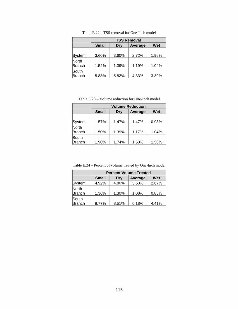
115

Table E.22 – TSS removal for One-Inch model

TSS Removal Small Dry Average Wet

System 3.60% 3.60% 2.72% 1.96% North Branch 1.52% 1.39% 1.19% 1.04% South Branch 5.83% 5.82% 4.33% 3.39%

Table E.23 – Volume reduction for One-Inch model

Volume Reduction Small Dry Average Wet

System 1.57% 1.47% 1.47% 0.93% North Branch 1.50% 1.39% 1.17% 1.04% South Branch 1.90% 1.74% 1.53% 1.50%

Table E.24 – Percent of volume treated by One-Inch model

Percent Volume Treated Small Dry Average Wet System 4.92% 4.80% 3.63% 2.67% North Branch 1.36% 1.30% 1.08% 0.85% South Branch 8.77% 8.51% 6.18% 4.41%

116

Table E.25 – Individual BMP treatment percentages for One-Inch Model

BMP Treatment Efficiencies Avg BMP ID Small Dry Average Wet Type

TP118b 98.97% 95.46% 88.86% 75.50% 82.18% Bioretention TP120b1 97.51% 94.37% 87.73% 74.27% 81.00% Bioretention TP120b2 97.50% 93.54% 86.81% 73.13% 79.97% Bioretention TP121 98.38% 94.19% 88.09% 74.66% 81.37% Bioretention TP101 98.22% 94.78% 88.00% 15.23% 51.62% Bioretention TP110b 97.20% 93.38% 85.25% 64.78% 75.01% Bioretention TP115b1 97.48% 94.14% 87.29% 74.51% 80.90% Bioretention TP115b2 96.50% 92.66% 84.18% 70.07% 77.12% Bioretention TP108 98.39% 94.30% 88.05% 74.82% 81.44% Bioretention TP106b2 96.64% 93.04% 84.36% 71.38% 77.87% Bioretention TP123b 97.00% 93.21% 84.99% 71.73% 78.36% Bioretention TP100 100.00% 99.76% 100.00% 95.95% 97.98% Porous Pavement TP112pp 100.00% 97.52% 94.87% 89.03% 91.95% Porous Pavement TP114pp 100.00% 97.34% 94.37% 71.54% 82.96% Porous Pavement TP123it 85.19% 80.12% 55.89% 38.28% 47.08% Infiltration Trench TP118inf 83.87% 76.73% 52.82% 34.83% 43.82% Infiltration Basin TP107 65.60% 45.24% 28.83% 17.73% 23.28% Infiltration Basin TP104 32.51% 34.79% 27.22% 19.30% 23.26% Wetland TP109 24.09% 24.40% 14.85% 9.63% 12.24% Grass Swale

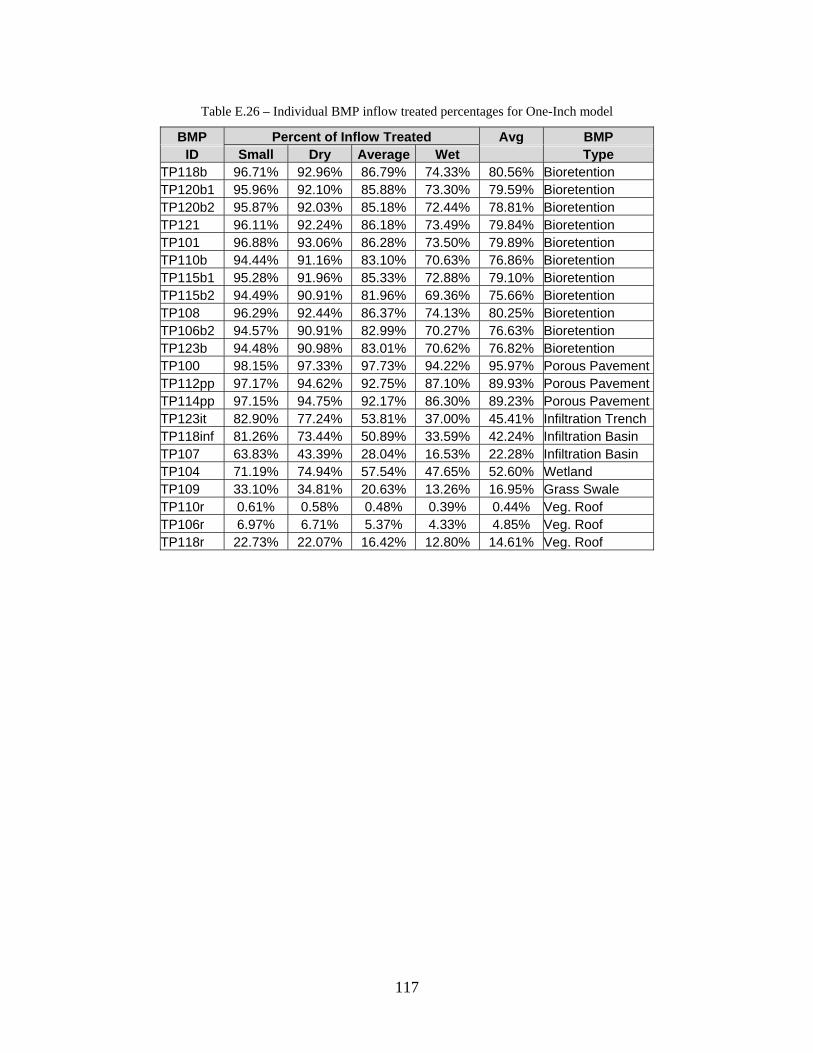
117

Table E.26 – Individual BMP inflow treated percentages for One-Inch model

BMP Percent of Inflow Treated Avg BMP ID Small Dry Average Wet Type

TP118b 96.71% 92.96% 86.79% 74.33% 80.56% Bioretention TP120b1 95.96% 92.10% 85.88% 73.30% 79.59% Bioretention TP120b2 95.87% 92.03% 85.18% 72.44% 78.81% Bioretention TP121 96.11% 92.24% 86.18% 73.49% 79.84% Bioretention TP101 96.88% 93.06% 86.28% 73.50% 79.89% Bioretention TP110b 94.44% 91.16% 83.10% 70.63% 76.86% Bioretention TP115b1 95.28% 91.96% 85.33% 72.88% 79.10% Bioretention TP115b2 94.49% 90.91% 81.96% 69.36% 75.66% Bioretention TP108 96.29% 92.44% 86.37% 74.13% 80.25% Bioretention TP106b2 94.57% 90.91% 82.99% 70.27% 76.63% Bioretention TP123b 94.48% 90.98% 83.01% 70.62% 76.82% Bioretention TP100 98.15% 97.33% 97.73% 94.22% 95.97% Porous Pavement TP112pp 97.17% 94.62% 92.75% 87.10% 89.93% Porous Pavement TP114pp 97.15% 94.75% 92.17% 86.30% 89.23% Porous Pavement TP123it 82.90% 77.24% 53.81% 37.00% 45.41% Infiltration Trench TP118inf 81.26% 73.44% 50.89% 33.59% 42.24% Infiltration Basin TP107 63.83% 43.39% 28.04% 16.53% 22.28% Infiltration Basin TP104 71.19% 74.94% 57.54% 47.65% 52.60% Wetland TP109 33.10% 34.81% 20.63% 13.26% 16.95% Grass Swale TP110r 0.61% 0.58% 0.48% 0.39% 0.44% Veg. Roof TP106r 6.97% 6.71% 5.37% 4.33% 4.85% Veg. Roof TP118r 22.73% 22.07% 16.42% 12.80% 14.61% Veg. Roof

118

Appendix F Continuous Simulation Pond Depths

119

0

1

2

3

4

5

6

7

8

0 50 100 150 200 250 300 350 400

Time (days)

Dep

th (f

t)

100-year Depth

10-year Depth

2-year Depth

Figure F.1 – Upper Francis Lane pond depths during Wet year

120

0

1

2

3

4

5

6

7

8

9

0 50 100 150 200 250 300 350 400

Time (days)

Dep

th (f

t)

100-year Depth

10-year Depth

2-year Depth

Figure F.2 – Lower Francis Lane pond depths during Wet year

121

0

1

2

3

4

5

6

7

0 50 100 150 200 250 300 350 400

Time (days)

Dep

th (f

t)100-year Depth

10-year Depth

2-year Depth

Figure F.3 – Upper Francis Lane pond depths during Average year

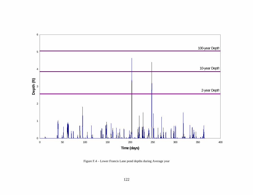
122

0

1

2

3

4

5

6

0 50 100 150 200 250 300 350 400

Time (days)

Dep

th (f

t)

100-year Depth

10-year Depth

2-year Depth

Figure F.4 – Lower Francis Lane pond depths during Average year