A C A D E M I A A N D C L I N I C

The Use of Predicted Confidence Intervals When Planning Experiments and the Misuse of Power When Interpreting Results Steven N. Goodman, MD, PhD, and Jesse A. Berlin, ScD

• Although there is a growing understanding of the importance of statistical power considerations when designing studies and of the value of confidence inter­vals when interpreting data, confusion exists about the reverse arrangement: the role of confidence intervals in study design and of power in interpretation. Confidence intervals should play an important role when setting sample size, and power should play no role once the data have been collected, but exactly the opposite procedure is widely practiced. In this commentary, we present the reasons why the calculation of power after a study is over is inappropriate and how confidence intervals can be used during both study design and study interpretation.

Ann Intern Med. 1994;121:200-206.

From Johns Hopkins University School of Medicine, Baltimore, Maryland; and the University of Pennsylvania School of Medi­cine, Philadelphia, Pennsylvania. For current author addresses, see end of text.

The increasing statistical sophistication of medical re­searchers has heightened their awareness of the impor­tance of having appropriate statistical power in a clinical experiment. Power is the probability that, given a speci­fied true difference between two groups, the quantitative results of a study will be deemed statistically significant. Freiman and colleagues (1) sensitized researchers to the possibility that many so-called "negative" trials of medical interventions might have too few participants to produce statistically significant findings even if clinically important effects actually existed. These authors calculated the sta­tistical power of 71 "negative" studies that compared two treatments. They showed that for most of the studies, the power to detect a 50% improvement in success rates was quite low. This kind of analysis has been applied in var­ious specialty fields, with similar results (2-6).

Studies with low statistical power have sample sizes that are too small, producing results that have high statistical variability (low precision). Confidence intervals are a con­venient way to express that variability. Numerous articles, commentaries, and editorials (7-13) have appeared in the biomedical literature during the past decade showing how confidence intervals are informative data summaries that can be used in addition to or instead of P values in reporting statistical results.

Although there is a growing understanding of the role of power in designing studies and the role of confidence

intervals in study interpretation, confusion exists about the reverse arrangement, the role of confidence intervals in designing studies and of power estimates in interpret­ing study findings. Confidence intervals should play an important role when setting sample size, and power should play no role once the data have been collected, but exactly the opposite is widely practiced. When "no significant difference" between two compared treatments is reported, a common question posed in journal clubs, on rounds, in letters to the editor, and in reviews of manu­scripts is, "What was the power of the study to detect the observed difference?" A widely used instrument for as­sessing the quality of a clinical trial penalizes studies if post hoc power calculations of this type are omitted (14), and reviews of the literature are frequently critical of the failure to include them (15, 16).

Although several writers (12, 17-19) have pointed out the error implicit in the concept of post hoc power, such caveats have not had great impact. This is perhaps be­cause the error implicit in post hoc power is created by a subtle inconsistency in the logic of standard statistical methods. This inconsistency derives from applying a pre-experiment probability of a hypothetical group of results to the one result that is observed. Most discussions of this problem focus on purported errors in interpreting statis­tical rules, rather than on the problems with the statistical framework itself. We elucidate the problems with the framework in the course of explaining why post hoc esti­mates of power are of little help in interpreting results and why the focus of attention should be exclusively on confidence intervals. In addition, we show how the size of a confidence interval can be predicted in the planning stages of an experiment and how that can be a great help in understanding the implications of different sample size choices.

Confidence Intervals

A confidence interval can be thought of as the set of true but unknown differences that are statistically compat­ible with the observed difference. The standard conven­tion for this statistical compatibility is the two-sided 95% confidence interval. A confidence interval is typically re­ported in the following way: "There was a 10% (95% CI, 2% to 18%) difference in mortality." This means that even though the observed mortality difference was 10% (for example, 70% compared with 60%), the data are statistically compatible with a true mortality difference as small as 2% or as large as 18%.

True differences that lie outside the 95% confidence interval are not impossible; they merely have less statis­tical evidence supporting them than values within it. The

200 © 1994 American College of Physicians

Downloaded From: http://annals.org/ by a Charite Campus User on 11/20/2012

choice of 95% as the standard convention is somewhat arbitrary and corresponds to the use of a threshold of P < 0.05 for statistical significance. However, a confidence interval should not be treated simply as a surrogate for a significance test, that is, to declare "nonsignificance" when the null hypothesis is included within it and to declare "significance" when it is not (20). The location and width of the confidence interval have important in­formation (9, 11).

Before the Experiment: The Proper Use of Statistical Power

The meaning of "power" before an experiment is straightforward. Suppose we are evaluating a medical treatment that has a 45% cure rate. A surgical procedure is proposed but because of the surgical morbidity, we judge that it would have to achieve a 70% cure rate (25 percentage points better than medical therapy) to justify its use. If we are designing a clinical trial to compare the two therapies, and the treatment difference was that big, 80 participants would have to be randomized to each therapy to produce a study with a 90% chance of achiev­ing a statistically significant difference. This "90% chance" is the power of the study with respect to an underlying cure rate difference of 25%. The jargon is that we have 90% power to "detect" a 25% difference. Conventionally, power should be no lower than 80% and preferably around 90%, akin to a diagnostic test with a sensitivity of 80% to 90%. For any given underlying difference, a larger sample size produces greater power.

Although the role of power in the planning stage of an experiment may be fairly clear, it comes with baggage that can lead to confusion when interpreting the results of that experiment. Implicit in its use is the assumption that we will report the results of a study only as "statistically significant" or "not statistically significant," without fur­ther detail. Although that is how medical research results are sometimes simplistically summarized, that is rarely the only information provided in a research report. Research­ers typically report at least the size of the observed effect (for example, "an average blood pressure decrease of 10 mm Hg") and the precise P value (for example, P = 0.03, not just P < 0.05). As we show in the next section, once that information is provided, neither power nor its con­comitant notion of "detecting a difference" remains a meaningful concept. Power is exclusively a pretrial con­cept; it is the probability of a group of possible results (namely, all statistically significant outcomes) under a specified alternative hypothesis. A study produces only one result. We discuss the methods that must be adopted after that result has been observed.

After the Experiment: The Improper Use of Statistical Power

The perspective after the experiment differs from that before the experiment simply because the result is known. That may seem obvious, but what is less apparent is that we cannot cross back over the divide and use pre-exper-iment numbers to interpret the result. That would be like

trying to convince someone that buying a lottery ticket was foolish (the before-experiment perspective) after they hit a lottery jackpot (the after-experiment perspective).

We will show the problem with combining those per­spectives by a close examination of the concept of "de­tection." This concept is derived from the field of signal detection, whose purposes differ somewhat from those in medical research. In the signal detection model, we are concerned with deciding whether there is a message within random noise; it is either there or it is not. Results fall into one of only two possible categories: "A signal is detected" or "a signal is not detected." The parallel with the "hypothesis test" paradigm of statistics is direct; we report that either a statistically significant result is ob­served (that is, the observed difference is distinguishable from random variation and the null hypothesis is rejected) or a statistically nonsignificant result is observed (that is, the observed difference cannot be distinguished from ran­dom variation and the null hypothesis is accepted).

Problems are produced when we apply this paradigm to medical research. We will continue with the previous ex­ample, in which there was 90% power to "detect" a 25% difference between two treatments, with n = 80 in each of the two groups. Suppose we observed a cure rate of 60/80 (75%) in one group and of 49/80 (61%) in the other, a difference of 14%. This has a P value of 0.06, not quite statistically significant at a = 0.05. There are two ways we can report this result, one in which the notion of "detec­tion" makes some sense, and one in which it does not. We could say simply that a statistically nonsignificant result was observed (P > 0.05) without reporting the ob­served 14% difference or the exact P value of 0.06. With this information, one would conclude that the true differ­ence was probably less than 25% because there was a 90% power chance of achieving statistical significance (that is, "detecting a difference") if a 25% true difference existed. Conversely, if statistical significance (P < 0.05) had been achieved, we would claim that the null hypoth­esis was unlikely because there was only a 5% chance of observing such a result if the null hypothesis were true. Thus, all the components of the sample size calculation— the detectable difference, the notion of "detection," power, and a—remain relevant for the interpretation of the result if we reduce it to just one of two possible outcomes. However, this relevance comes at a steep price: It means that our degree of confidence in the "no differ­ence" conclusion is the same for every nonsignificant result, and our confidence in a "some difference" conclusion is the same for every significant result.

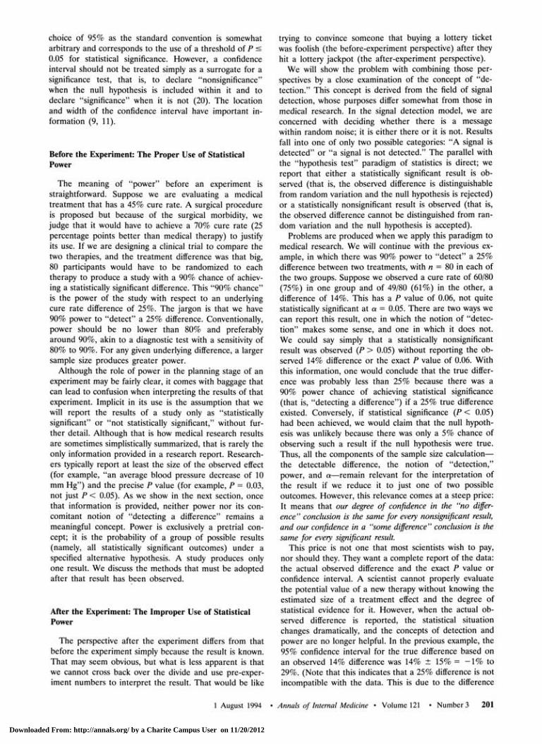
This price is not one that most scientists wish to pay, nor should they. They want a complete report of the data: the actual observed difference and the exact P value or confidence interval. A scientist cannot properly evaluate the potential value of a new therapy without knowing the estimated size of a treatment effect and the degree of statistical evidence for it. However, when the actual ob­served difference is reported, the statistical situation changes dramatically, and the concepts of detection and power are no longer helpful. In the previous example, the 95% confidence interval for the true difference based on an observed 14% difference was 14% ± 15% = - 1 % to 29%. (Note that this indicates that a 25% difference is not incompatible with the data. This is due to the difference

1 August 1994 • Annals of Internal Medicine • Volume 121 • Number 3 201

Downloaded From: http://annals.org/ by a Charite Campus User on 11/20/2012

in conventions we use for power [one-sided, 80% to 90%] and confidence intervals [two-sided, 95%]). If we had observed no difference between the therapies, P = 1.0, we would report that the true difference was probably within the 95% confidence interval of 0 ± 15%= - 1 5 % to 15%. A true 25% difference would be extremely implau­sible based on that result. Depending on such factors as relative treatment costs, toxicity, and other background information, one might make very different recommenda­tions based on those two nonsignificant results.

The concepts of "power" or "detection" are of no help in distinguishing those results, because both results are "nonsignificant." The power of an experiment is the pre­trial probability of all nonsignificant outcomes taken to­gether (under a specified alternative hypothesis), and any attempt to apply power to a single outcome is problem­atic. When people try to use power in that way, they immediately encounter the problem that there is not a unique power estimate to use; there is a different power for each underlying difference. Does one say that a non­significant result rules out a 25% difference with 90% confidence (because there was 90% power for a 25% difference); or that it rules out a 21% difference with 80% confidence; or that it rules out a 15% difference with 50% confidence?

To eliminate this ambiguity, some researchers calculate the power with respect to the observed difference, a num­ber that is at least unique. This is what is called the "post hoc power." In the example, the post hoc power with respect to the observed difference of 14% is 45%, quite low. The unstated rationale for the calculation is roughly as follows: It is usually done when the researcher believes there is a treatment difference, despite the nonsignificant result. She uses the 45% power to prove that the study was too small to "detect" a 14% difference, and therefore the experiment's "negative" verdict is not definitive, that is, it does not eliminate the possibility of the 14% differ­ence being real.

There are two reasons why this exercise is unhelpful. First, it will always show that there is low power (< 50%) with respect to a nonsignificant difference (21), making tautological and uninformative the claim that a study is "underpowered" with respect to an observed nonsignifi­cant result. Second, its rationale has an Alice-in-Wonder-land feel, and any attempt to sort it out is guaranteed to confuse. The conundrum is the result of a direct collision between the incompatible pretrial and post-trial perspec­tives. The pretrial paradigm, with its focus on "deciding" between the null and alternative hypotheses, dictated that the 14% observation, and all other nonsignificant results, produce acceptance of the null hypothesis of a zero true difference. But common sense tells us that 14% is the best estimate of the true difference, even if the statistical ev­idence to distinguish it from a zero difference is not definitive. Knowledge of the observed difference naturally shifts our perspective toward estimating differences, rather than deciding between them, and makes equal treatment of all nonsignificant results impossible. Once the data are in, the only way to avoid confusion is to not compress results into dichotomous significance verdicts and to avoid post hoc power estimates entirely.

The Connection with P Values

Arguments similar to those above can and have been applied to P values (22), which are defined as the prob­ability of the observed data, plus more extreme data, under the null hypothesis. A P value is to a type I error exactly as "1 - post hoc power" is to a type II error; that is, where " 5 % " is almost always the type I error rate set before the experiment; after the experiment, the P value is frequently described as the "observed" type I rate (23) or, in other words, the type I error rate with respect to the observed difference. The notion of the P value as an "observed" type I error suffers from the same logical problems as post hoc power. Once we know the observed result, the notion of an "error rate" is no longer mean­ingful in the same way that it was before the experiment. Much has been written about the problem of interpreting the P value as an "observed error rate," either by expli­cating and exposing it (22, 24-30) or by gently steering students of medical statistics away from improper inter­pretations and toward at least usable ones (31).

The Role of Confidence Intervals in Interpreting Results

We have already shown in the previous examples how confidence intervals can be used to interpret a result. As mentioned earlier, the 14% result (CI; - 1 % to 29%) did not statistically rule out either a 0% or 25% difference. Often, when confronted with a result like this, an author will state in the discussion section that "the study may have had too little power to have detected a small differ­ence," leaving ambiguous what differences the study ac­tually ruled out and making it appear as though the excluded differences are a function of the design, not the results. Such fuzziness is unwarranted; the confidence in­terval tells us what differences are and are not statistically ruled out based on what was actually observed.

Another phrase that researchers often use to describe nonsignificant results is that "statistical significance was not achieved because of small sample size." When re­searchers say this, they are implicitly claiming that they believe the observed effect to be true, despite the failure to statistically exclude a zero effect. Nothing is wrong with this statement, except that it is never justified by the data alone. If we somehow knew that a small sample size was the only reason significant results were not achieved, then all experiments could be done with n = 2, and we could always make that claim. If an author believes that an observed nonsignificant difference is real, then that belief must be founded on the combination of external evidence (for example, biological reasoning and other studies) with the evidence from this experiment. The readers can then judge the strength of the overall evidence. Confidence intervals address the only question that can be properly asked of the data: With the given sample size and given observed effect, which true effects are statistically compat­ible with the data and which are not?

Bayesian and Likelihood Methods

Unfortunately, even confidence intervals do not tell us, "given the observed effect, how probable is it that the true effect is greater than 14%" or "given the data, how

202 1 August 1994 • Annals of Internal Medicine • Volume 121 • Number 3

Downloaded From: http://annals.org/ by a Charite Campus User on 11/20/2012

much more evidence is there for a 14% difference as opposed to no difference?" These are the questions in which most researchers are interested, but they cannot be formally answered with conventional (that is, "frequen­tist") statistical methods. They require Bayesian or likeli­hood approaches (30, 32-37). A full exposition of these methods is beyond the scope of this paper, but they will be described briefly. Likelihood methods allow calculation of the relative amount of statistical evidence for any two statistical hypotheses, for example, the null hypothesis and the hypothesis that a "clinically important difference" ex­ists. The measure of evidence is the likelihood ratio, defined as the probability of the observed data under one hypothesis divided by the probability of the data under another hypothesis (33, 34, 38).

Bayesian methods add a measure of "prior belief or "prior evidence" to the likelihood ratio, and, via Bayes theorem, they estimate the posterior probabilities of var­ious true differences, based on the data. These Bayesian posterior probabilities are exactly what scientists want, but because prior belief can vary among persons, these meth­ods are sometimes described as "subjective" or "nonsci-entific" and are compared unfavorably with conventional statistics. We will not enter into this debate, except to note that conventional statistics have many subjective el­ements, like the conventions of the 95% confidence in­terval (instead of the 90% or 99% confidence interval) or the P < 0.05 threshold (instead of 0.10 or 0.01). By de­fining certain arbitrary standards as "conventions," the subjectivity is suppressed (25, 28).

Even if we do not use likelihood or Bayesian methods, those perspectives can be enormously useful in making sense of conventional statistical indices. Technically, a 95% confidence interval is the result of a procedure that should include the true value 95% of the time. From this technical perspective, we cannot say that any one confi­dence interval has a 95% chance of including the true value. This subtle distinction is confusing to researchers. From a likelihood perspective, confidence intervals can be reinterpreted as we have defined them in this article—as the set of true values that are statistically compatible with the observed data. Similarly, from a Bayesian perspective, we can interpret a confidence interval as having a 95% chance of including the true value if the information from the experiment is far greater than information from out­side the experiment. These are more intuitive and useful working definitions than the frequentist ones. A P value also has some useful likelihood and Bayesian interpreta­tions. These include viewing it as a lower limit of the probability that the effect is in a direction opposite to the one observed (39, 40).

Because medical researchers are more familiar with confidence intervals than likelihood ratios or Bayesian probabilities, we continue with a discussion of how con­fidence intervals can be used to help plan experiments.

Sample Size Calculation Using Predicted Confidence Intervals

Precision (defined as the width of the 95% confidence interval) and power are linked to sample size and so are mathematically related to each other. For any given power and "clinically important difference," we can pre­

dict before an experiment approximately how precise the results will be. The Appendix shows the derivation of the following simple rule-of-thumb relations.

Equation 1

Predicted 95% CI = observed difference ± 0.7 A080

= observed difference ± 0.6 A0 9 0

where A0 80 = true difference for which there is 80% power A0 90 = true difference for which there is 90% power

Both of these formulae yield the same result. More detailed discussions of this relation are found in Bristol (41). The importance of using predicted confidence inter­vals is that they give medical researchers a way to discuss the implications of a sample size in units that have mean­ing to them. Many clinicians or reviewing bodies do not know how to debate "power" but can understand and discuss the implications of measurement accuracy being within 50%.

A typical sample size consultation often resembles a ritualistic dance. The investigator usually knows how many participants can be recruited and wants the statis­tician to justify this sample size by calculating the differ­ence that is "detectable" for a given number of partici­pants rather than the reverse. The statistician typically will not use less than 80% power in the calculations, mainly because, by convention, anything lower than that will be questioned. Because no guidelines exist about which "clinically important difference" should be used in the calculation, often anything can pass muster. The "detect­able difference" that is calculated is typically larger than most investigators would consider important or even likely. But this "detectable difference" is usually not com­mented on by reviewing bodies and does not have to be quoted when the results of the study are analyzed, so researchers will often accept large differences for the pur­pose of getting a proposal approved. The result of this practice is that most clinical experiments are too small, and the journals are filled with a plethora of reports of clinically important but statistically nonsignificant effects, keeping persons who do meta-analysis in business (42).

Maintaining the focus on predicted confidence intervals can make researchers understand more clearly the real consequences of this sample size game. It will clearly show that the effect of choosing too large a "detectable difference" is to yield outcomes with confidence intervals so wide that even a zero observed effect might not rule out a clinically important difference. In other words, the results are highly likely to be inconclusive (43).

Using the previous example, in which the sample size of 80 in each group produced 90% power to detect a dif­ference of 25%, we can calculate (using Equation 1) that a result would have a predicted precision (95% confi­dence interval width) of about ± 0.6 X 25% = ± 15%. (15% also represents the smallest observed difference that is statistically significant.) This is a number whose impli­cations can be easily communicated. Figure 1 (top) shows what that degree of imprecision means for several hypo­thetical results: a zero difference, a difference near the borderline of significance (15%), and the "difference of

1 August 1994 • Annals of Internal Medicine • Volume 121 • Number 3 203

Downloaded From: http://annals.org/ by a Charite Campus User on 11/20/2012

Figure 1. Predicted 95% confidence intervals. Top. Predicted 95% confidence intervals for hypothetical findings of 0%, 15%, and 25% differences when the sample size is set with power of 90% for an absolute difference of 25% between two treatments {see text). Bottom. Predicted 95% confidence intervals for find­ings of 0%, 15% and 25% differences when the sample size is set with power of 90% for an absolute difference of 10% between two treatments {see text).

interest" (25%). Even if exact equivalence is observed, differences up to 15% cannot be excluded. If the real threshold for clinical importance was 25%, this would not be of great concern because the confidence limits around the zero difference exclude a difference as large as 25%. But typically the real difference of interest is less than that used in the sample size calculation. If the smallest clinically important difference was actually 10%, none of those 95% confidence intervals would convincingly rule it out.

If we used 10% as the detectable difference in the sample size calculation, the predicted precision would be ± 0.6 X 10% = ± 6% (Figure 1, bottom). We see im­mediately from the figure that the discrimination between findings of 0% and 15% difference is sharper. The confi­dence interval associated with a zero difference now points clearly to a clinically unimportant effect, whereas the confidence interval around 15% makes it highly un­likely that there is a trivial effect. This metric also allows us to compare various power-difference pairings. The dif­ference between having 70% power for a 7.5% difference, 80%) for an 8.4%) difference, or 90% for a 10%) difference is not obvious, and it is not apparent what should be reported in a proposal. When it is noted that all of these produce the same degree of precision, the discussion can focus on that, instead of which combination of power and difference to report.

Pointing out that an observed zero difference cannot exclude differences up to 15% or that an observed 10% difference cannot exclude differences up to 25% often will give a researcher pause, whereas the choice of a 25% "difference of interest" may not. In our experience, ex­pressing the implications of sample size calculations in the same language as is used in a published paper, instead of the language of power and detectable differences, helps researchers to understand the implications more clearly and take them more seriously. This, in turn, can produce

meaningful discussions about the aims of the study, which power considerations rarely seem to inspire.

We are not recommending the abandonment of con­ventional sample size formulae in favor of ones based solely on predicted precision (44-47). When this is done, a tendency exists to make the precision exactly equal to the difference of interest, which produces experiments with 50% power (19). Rather, as several others (19, 41, 48) have also recommended, one should use the standard formulae and then look at their implications in terms of precision.

The Purpose of Presenting Sample Size and Power Calculations

What are the reasons to present sample size calcula­tions in a published paper, a practice that many statistical guidelines recommend (49)? We believe they are limited. One purpose is to tell us the appropriate sample size for future experiments. This would discourage the incorrect practice of justifying a sample size by matching the size of previous studies that have achieved statistical significance. If we choose sample sizes in this way, the power can be as low as 50% even if the previously observed differences are true (21). The way to use previous studies is to use the observed differences as a guide to the true difference as well as to statistical variability. Reporting sample size calculations can give a sense of how well the study was planned and executed (by matching the goals against the enrollment) and provides a clue to the quantitative so­phistication of the researcher. Because the sample size calculation must include many factors that are dealt with later in the analysis, a careful and sophisticated presen­tation of sample size considerations can increase our con­fidence that difficult analytical issues were handled appro­priately.

We must emphasize that for statistical interpretation of the results, however, the details of a sample size calcula­tion are of no help. Some claim they are useful because they show the investigator's previous opinions as to the most likely effect. But no guarantee exists that the differ­ence used in the sample size calculation will reflect any­one's opinion. What if investigators plan to have 50% power for a real difference of interest but then quote the larger difference associated with 80% power, or what if the sample size was based not on a difference but on the availability of participants? In any case, the investigator's previous opinions are important only insofar as they are based on objective evidence. If they are, this evidence should be presented as part of the discussion so readers can interpret for themselves the observed effect in light of previous evidence. If they are not, then the opinions are not important.

Conclusion

If low power or a hopelessly optimistic effect size is used in a sample size calculation, this will be reflected in an inability after the trial to distinguish between clinically important and unimportant results, which will be ex­pressed in the form of wide confidence intervals. Thus, a price is paid if the previous sample size estimation pro­cedure is treated as a pro forma exercise. The approxi-

204 1 August 1994 • Annals of Internal Medicine • Volume 121 • Number 3

Downloaded From: http://annals.org/ by a Charite Campus User on 11/20/2012

mate size of the confidence interval after the experiment can be predicted before the experiment, and this predic­tion should supplement traditional sample size calcula­tions and should be reported in proposals. For interpre­tation of observed results, the concept of power has no place, and confidence intervals, likelihood, or Bayesian methods should be used instead.

Appendix: Derivation of Equation 1

When the standard errors of the difference are equal under the null and alternative hypotheses, and outcomes approximately Gaussian, the basis of standard sample size formula is to make the difference of interest, A, equal to Za/2 + Zp standard errors from the null hypothesis. This corresponds to the equation:

A, _ p = (Za^ + Zp) x standard error

Where:

1 - ]8 = power A! _ p = difference that can be detected with power 1-/3. Za/2 - Z-score associated with two-sided type I error of a. Zp = Z-score associated with one-sided type II error of /3.

For a one-sided power of 80% and two-sided a = 5%, Za/2 + Zp - 1.96 + 0.84 = 2.8. This means that when the power is 80%, the difference of interest, A080, is 2.8 standard errors from the null hypothesis. The predicted 95% confidence interval equals the observed difference ± 1.96 standard errors, but we can re­place the standard error with A080/2.8:

Predicted 95% CI = observed difference ± 1 .96-^ 2.8

= observed difference ± 0.7 A080

For one-sided power = 90%, Za/2 + Zp = 1.96 + 1.28 = 3.24. Thus, the standard error also equals A()90/3.24. Substituting that into the confidence interval equation, we get:

A() 9() Predicted 95% CI = observed difference ±1.96 —

3.24 = observed difference ± 0.6 A090

Caveat: When sample sizes are small (total n <20) and the outcomes are Gaussian, then the appropriate thresholds from the Student f-distribution should be used in place of the Gaussian Za/2 and Zp. In the case of proportions, variances can differ substantially under the null and alternative hypotheses when both proportions are not between 1/4 and 3/4, and the above equa­tions apply only approximately. See Bristol (41) for exact equa­tions.

Requests for Reprints: Steven Goodman, MD, PhD, Oncology Center, Division of Biostatistics, Johns Hopkins University, 550 North Broadway, Suite 1103, Baltimore, MD 21205.

Current Author Addresses: Dr. Goodman: Oncology Center, Division of Biostatistics, Johns Hopkins University, 550 North Broadway, Suite 1103, Baltimore, MD 21205. Dr. Berlin: University of Pennsylvania, Center for Clinical Epidemiology and Biostatistics, 321R Nursing Education Building, 420 Service Drive, Philadelphia, PA 19104-6095.

References

1. Freiman JA, Chalmers TC, Smith H Jr, Kuebler RR. The importance of beta, the type II error and sample size in the design and interpre­tation of the randomized clinical trial. Survey of 71 negative trials. N Engl J Med. 1978;299:690-4.

2. Edlund MJ, Overall JE, Rhoades HM. Beta, or type II error in psychiatric controlled clinical trials. J Psychiatr Res. 1985;19:563-7.

3. Brown CG, Kelen GD, Ashton JJ, Werman HA. The beta error and sample size determination in clinical trials in emergency medicine. Ann Emerg Med. 1987;16:183-7.

4. Dyken ML. Transient ischemic attacks and aspirin, stroke and death; negative studies and Type II error [Review]. Stroke. 1983;14:2-4.

5. Raju TN, Langenberg P, Sen A, Aldana O. How much 'better' is good enough? The magnitude of treatment effect in clinical trials. Am J Dis Child. 1992;146:407-11.

6. Ottenbacher KJ, Barrett KA. Statistical conclusion validity of rehabil­itation research. A quantitative analysis. Am J Phys Med Rehabil. 1990;69:102-7.

7. Berry G. Statistical significance and confidence intervals [Editorial]. Med J Aust. 1986;144:618-9.

8. Braitman LE. Confidence intervals extract clinically useful information from data [Editorial]. Ann Intern Med. 1988;108:296-8.

9. Braitman LE. Confidence intervals assess both clinical significance and statistical significance [Editorial]. Ann Intern Med. 1991;114:515-7.

10. Gardner MJ, Altman DG. Confidence intervals rather than P values: estimation rather than hypothesis testing. Br Med J. 1986;292:746-50.

11. Simon R. Confidence intervals for reporting results of clinical trials. Ann Intern Med. 1986;105:429-35.

12. Smith AH, Bates MN. Confidence limit analyses should replace power calculations in the interpretation of epidemiologic studies. Epidemiol­ogy. 1992;3:449-52.

13. Rothman KJ. A show of confidence [Editorial]. N Engl J Med. 1978; 299:1362-3.

14. Chalmers TC, Smith H Jr, Blackburn B, Silverman B, Schroeder B, Reitman d, et al. A method for assessing the quality of a randomized control trial. Controlled Clin Trials. 1981;2:31-49.

15. Evans M, Pollock AV. A score system for evaluating random control clinical trials of prophylaxis of abdominal surgical wound infection. Br J Surg. 1985;(72):256-60.

16. Moskowitz G, Chalmers TC, Sacks HS, Fagerstrom RM, Smith H Jr. Deficiencies of clinical trials of alcohol withdrawal. Alcohol Clin Exp Res. 1983;7:42-6.

17. Detsky AS, Sackett DL. When was a 'negative' clinical trial big enough? How many patients you needed depends on what you found. Arch Intern Med. 1985;145:709-12.

18. Fletcher RH, Fletcher SW, Wagner EH. Clinical Epidemiology: The Essentials. 2nd ed. Baltimore: Williams & Wilkins; 1998:1-246.

19. Greenland S. On sample-size and power calculations for studies using confidence intervals. Am J Epidemiol. 1988;128:231-7.

20. Poole C. Beyond the confidence interval. Am J Public Health. 1987; 77:195-9.

21. Goodman SN. A comment on replication, P-values and evidence. Stat Med. 1992;11:875-9.

22. Goodman SN. P-values, hypothesis tests, and likelihood: implications for epidemiology of a neglected historical debate (with commentary and response). Am J Epidemiol. 1993;137:485-96.

23. Bickel P, Docksum K. Mathematical Statistics. San Francisco: Holden-Day; 1977:171-2.

24. Oakes M. Statistical Inference: A Commentary for the Social Sciences. New York: Wiley; 1986.

25. Good I. Good Thinking: The Foundations of Probability and its Ap­plications. Minneapolis: University of Minnesota Press; 1983.

26. Johnstone D. Tests of significance in theory and practice. The Statis­tician. 1986;35:491-504.

27. Royall R. The effect of sample size on the meaning of significance tests. Am Statist. 1986;40:313-5.

28. Berger J, Berry D. Statistical analysis and the illusion of objectivity. American Scientist. 1988;76:159-65.

29. Berger J, Wolpert R. The Likelihood Principle. IMS Series. 1988;6. 30. Diamond GA, Forrester JS. Clinical trials and statistical verdicts:

probable grounds for appeal. Ann Intern Med. 1983;98:385-94. 31. Ingelfinger JA, Mosteller F, Thibodeau L, et al. Biostatistics in Clinical

Medicine. New York: Macmillan; 1987. 32. Edwards W, Lindman H, Savage L. Bayesian statistical inference for

psychological research. Psych Rev. 1963;70:193-242. 33. Edwards A. Likelihood. Cambridge: Cambridge University Press; 1972. 34. Goodman SN, Royall R. Evidence and scientific research. Am J Public

Health. 1988;78:1568-74. 35. Box G, Tiao G. Bayesian Inference in Statistical Analysis. New York:

John Wiley; 1973. 36. Barnett V. Comparative Statistical Inference. New York: Wiley; 1982. 37. Spiegelhalter DJ, Freedman LS. A predictive approach to selecting

the size of a clinical trial, based on subjective clinical opinion. Stat Med. 1986;5:1-13.

38. Good I. Probability and the Weighing of Evidence. New York: Charles Griffin & Co; 1950.

39. Casella G, Berger R. Reconciling bayesian and frequentist evidence in the one-sided testing problem. J Am Statist Assoc. 1987;82:106-11.

40. Pratt J. Bayesian interpretation of standard inference statements. Journal of the Royal Statistical Society, B. 1965;27:169-203.

41. Bristol DR. Sample sizes for constructing confidence intervals and testing hypotheses. Stat Med. 1989;8:803-11.

42. Yusuf S, Collins R, Peto R. Why do we need some large, simple randomized trials? Stat Med. 1984;3:409-20.

43. Simon R, Wittes RE. Methodologic guidelines for reports of clinical trials. Cancer Treat Rep. 1985;69:1-3.

1 August 1994 • Annals of Internal Medicine • Volume 121 • Number 3 205

Downloaded From: http://annals.org/ by a Charite Campus User on 11/20/2012

44. Beal SL. Sample size determination for confidence intervals on the population mean and on the difference between two population means. Biometrics. 1989;45:969-77.

45. McHugh RB, Le CT. Confidence estimation and the size of a clinical trial. Controlled Clin Trials. 1984;5:157-63.

46. Satten GA, Kupper LL. Sample size requirements for interval estima­tion of the odds ratio. Am J Epidemiol. 1990;131:177-84.

47. Gordon I. Sample size estimation in occupational mortality studies with use of confidence interval theory. Am J Epidemiol. 1987;125:158-62.

48. Daly LE. Confidence intervals and sample sizes: don't throw out all your old sample size tables. BMJ. 1991;302:333-6.

49. Bailar JC 3d, Mosteller F. Guidelines for statistical reporting for medical journals. Amplifications and explanations. Ann Intern Med. 1988;108:266-73.

What used to be called judgement is now called prejudice, and what used to be called prejudice is now called a null hypothesis It is dangerous nonsense (dressed up as 'the scientific method'), and will cause much trouble before it is widely appreciated as such.

A.W.F. Edwards Likelihood Cambridge, Cambridge University Press, 1972, p. 180

Submissions from readers are welcomed. If the quotation is published, the sender's name will be acknowl­edged. Please include a complete citation, as done for any reference.—The Editors

2 0 6 1 August 1994 • Annals of Internal Medicine • Volume 121 • Number 3

Downloaded From: http://annals.org/ by a Charite Campus User on 11/20/2012