THE USE OF HERMITIAN TIMOSHENKO FINITE ELEMENT FOR …

Proceedings of the 8th ASAT Conference, 4-6 May 1999 Paper SM-15 405

Military Technical College Kobry Elkobbah,

Cairo, Egypt

4P11‘

T nispioA IIA IF

8th International Conference on Aerospace Sciences &

Aviation Technology

THE USE OF HERMITIAN TIMOSHENKO FINITE ELEMENT FOR THE DYNAMIC ANALYSIS OF A LIGHTWEIGHT MANIPULATOR

M. M. Hegaze*, S. Kyriacou*, & A. EI-Zafrany*

ABSTRACT

Literature studies have demonstrated that lightweight manipulators of highspeed should be designed with the effects of shear deformation and rotary inertia being taken into consideration, especially for short beams. It has been found that Lagrangian Timoshenko beam elements are overstaff for small thickness, and such elements cannot be accurately employed for thin beams. This phenomenon is referred to as shear locking. This parametric study demonstrates the advantages of using a Hermitian Timoshenko finite element for the dynamic analysis of a lightweight manipulator. The Lagrangian principle is used for the derivation of the governing differential equations for the beam element. A computer program is developed to solve the proposed model and to easily accommodate any future developMents. The accuracy of the proposed model has been verified through the comparison of the dynamic response with two published models, one of them is based on assumed mode method and the other one is based on an isoparametric finite element method.

1. INTRODUCTION

The use of robotic manipulators in industrial applications has long been recognised. Their use allows the automation of manufacturing processes, the remote operation of machines in hazardous environments etc. The performance of such manipulators in terms of accuracy of movement, location and speed of response depends upon the inertia of the system. Due to their size, manipulators make a substantial contribution to the inertia of such assemblies.

In order to increase the productivity, robotic manipulators must function at higher speeds and enhanced accuracy. The manipulators, which are characterised by their large structural size and slow operational speed, may be considered rigid. The requirements of feasible driving power, weight and material cost of the rigid manipulator will be impracticable. Lightweight manipulators are a more natural way to reduce the driving power and increase the operational speed. The lightweight design requires that the flexibility effects must be taken into consideration. There are two kinds of problems introduced if the flexibility effect is not included in the mathematical model. The first one is found in the torque requirement for the motors and the second one results in the positioning inaccuracy of the end-effector.

*School of Mechanical Engineering, Cranfield University, Cranfield, Bedford, MK43 OAL, UK.

Proceedings of the Stn ASAT Conference, 4-6 May 1999

Paper SM-15 406

There have been several approaches to represent the flexible model of robotic manipulators. Book [1] modelled an elastic chain with an arbitrary number of links and joints. This model was limited in the assumption that the mass of the manipulator is negligible compared to the mass of the payload. This assumption is true for a space manipulator, which is light and operates at low speeds.

Petroka and Chang [2] have experimentally validated the accuracy of the Equivalent Rigid Link System (ERLS) dynamic model. The model was tailored to a single-link flexible arm system in which a hydraulic actuation was utilised, and the motion of the arm was limited to a vertical plane. The flexible dynamics has been studied by two methods, the first one is the assumed mode method [2, 3]. The main disadvantage of this method is the selection of modes if the links are of non-regular cross-section. The second one is the finite element method [5, 6]. In Parveen and Anand [4], the dynamic equations of flexible manipulators have been formulated using the Galerkin method and the axial strains are used as one of the nodal coordinates. In SMAILI [5], the dynamic behaviour of a planar manipulator is introduced by a three-node isoparametric finite element, and has only three shape functions to represent the nodal displacements, one for each node. In this paper, the dynamic equations of lightweight manipulators have been formulated, based on Hermitian interpolation functions and by using Lagrangian equations of motion. The nodal displacements of the element are taken as generalised coordinates, where the Rigid Body motion is represented by the joint angle 0. The stiffness and mass matrix of a two-node beam element are obtained where the shear deformation and rotary inertia effects are taken into consideration. A computer simulation program has been developed to solve this model.

2. KINEMATIC RELATIONS

The kinematic relations describe the overall motion of a beam which is subdivided into a Rigid Body Motion, represented by the joint angle 0, and an Elastic Motion, represented by the nodal displacements u. The kinematic properties of the link are described by the kinematics of its nodes. The kinematic relations employed for the approach, introduced here, are similar to these used by Ref. [3], which can be summarised as follows:

a=ar +Q u+R u+u (1)

where a is the absolute acceleration vector of the element nodes with respect to inertial coordinate frame OXYZ, ar is the acceleration associated with the rigid rotation,

u ,u are the relative velocity and acceleration of the node with respect to the local frame oxyz, Cg, R are 6x6 matrices which are function of the rigid body motion.


0

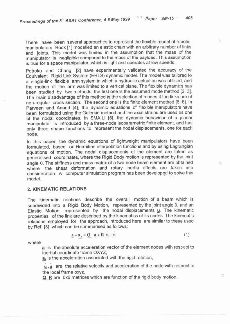
Fig.1. Geometry of two-node beam element

3. NODAL DISPLACEMENTS

The element nodal displacements are chosen to represent the axial, transverse and rotary displacements of the elastic beam at any node. The nodal displacement vector, of a two-node beam element, as shown in Fig. (1), can be defined at an instant of time t as follows:

Se (t)= { 11(t) S (01 (2) where

U(t) Ui V1 q U2 V2 (P2 8(t) ={ Wi 4/2 } u is the axial displacement of the node, v is the transverse displacement of the neutral axis at the node, cp is the slope angle of the neutral axis at the node, w Is the angle due to shear effects, which is defined as follows [6]:

av 41= - ex

According to the definition of nodal displacements, the displacements at any point, inside the element, can be expressed in terms of nodal parameters and shape functions as follows:

(9 The axial displacement u and the shear angle xi/ are assumed to obey Lagrangian interpolation [6]: u(x,t) = N1 ul(t) + N4 u2(t) (6) W (x,t) = Ni W1(t) + N4 w2(t) (7) where N1=1-t, N4= 4

(3) (4)

(5)

Proceedings of the 8th ASAT Conference, 4-6 May 1999

Paper SM-15 408

(-) The transverse displacement v(x) is assumed to obey Hermitian interpolation [6]: v(x,t) = N2 Vi + N3 ( (P1 - ) N5 v2 + N6 ( (P2 )

(8)

where N2 = 1- 3 42 + 2 43 N3 = L (4 - 2 42 4- (9)

N5 = 342 _ 2e N6 = L (4 - 242 + 43)

and 4 = x L d4 = dx/L (10)

(L)

The slope angle cp is defined as: av

(P= —ax Hence, the displacement components at any point (x,y,z) inside a beam deformed in the x-y plane due to the axial forces, shear forces and bending moments, can be approximated at an instant of time t as follows:

u(x,y,z,t) = u(x,t) - y 9(x,t) v(x,y,z,t) = v(x,t) (12) w(x,y,z,t) = 0

4. STIFFNESS MATRIX

A two-node beam element as shown in Fig.(1) where the x-axis is the beam neutral axis, and the beam is deformed in the x-y plane. Some assumptions, taken into consideration, are similar to those used by [6], which can be summarised as follows: (i) Lateral deformations are small compared with beam thickness, (..,) The beam material is homogenous, isotropic, and linearly elastic, (c) Normals to the neutral axis before deformation remain straight but not

necessarily normal to the neutral axis after deformation, (,) Stresses normal to the neutral axis are negligible.

Using the strain-displacement relations, the strain components can be obtained from displacement components given by equations (12), as follows

au ac0 E x = (13)

ax and the average value of shear strain yxy at x based on the given assumptions is given as:

- av rx = ax -

Hence, the vector of the relevant strain components can be defined as follows: = Ex yxY

(14)


Employing equations (6), (7), (8) and (11), the vector of strain, at any point inside the element, can be expressed in the following matrix form:

E _(8 - fla ) 8„

where

Pla [Ni

0

0

0

0

0

N4

0

0

0

0

0

0

0

0]

0

B= [0 yN; yN13 0 yN; yN6 y(N, -N;) Y (\14. - N 6)1 0 0 0 0 0 0 N1 N4

The stress components, at any point (x,y,z) inside the beam, can be defined as follows:

6x = E Ex

and the average value of shear stress Txy is given as: txy = G k yxy

where the shear factor k, for different cross-section geometries, is given by Cowper [7] and it is equal to 5 / 6 for rectangular sections. Hence, the vector of the relevant stress components can be defined as follows:

= ax txy

=( Ea,- 111 ) where

B,_

[0 yEN;

0 0

yEN3 0

0 0

yEN; 0

- yEN6 0

yE(N, -N;) GicNi

yE(N:i -N6) GIN 4

The total potential energy of the element is defined by means of the following expression:

X = U W (15) where U is the element strain energy, and W is the work done by,the applied forces. The strain energy for a linearly elastic material can be defined as follows:

U = —1 DT dxdydz

And for the given element, it can be shown that:

U= 2 — 8.er ( gi - )T E - )dxdydz ]Se (16)

Notice also that 11 dx dy = A the cross-section area cross section at x

if y2 dy dz = 1,(x), the second moment of area. cross section at x

The values of the nodal forces are defined such that the work done by the actual applied forces is equivalent to the work done by nodal forces i.e. ,‘

= 8 eT Fe (17)

Proceedings of the Stn ASAT Conference, 4-6 May 1999 Paper SM-15 410

Hence, substituting from equations (16) and (17) into (15), it can be deduced that:

1 T r x - 2 8 diff ( gh - I131 )T ( E B, - B3 ) dx dy dz 18. - 81; Fe

Applying the minimum total potential energy theorem the following matrix equation can be deduced:

K Eic = Fe where

= lJJJ (B, - B )T E - B3 ) dx dy dz

The previous stiffness matrix is of order 8x8, and it is useful to eliminate the parts which correspond to the y effects. The strain energy of the element can be expressed as follows:

u = 45.1 Kll K12 111 2 K21 K22 8

If 8 is assumed to minimise the strain energy, i. e. au

= o

it can be shown that: 8 = T u where T = K22-1 ni and U= 1 uT K u

2 — where K. is the condensed stiffness matrix defined as follows:

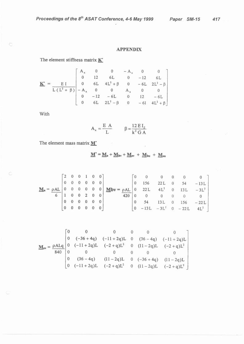
K`= — T explicit expression of K* is given in the Appendix.

(18)

5. MASS MATRIX

The velocity components at any point (x,y,z) inside the beam can be defined at an instant of time t by taking the first derivative of equations (12) with respect to

time, and they can be expressed in terms of a nodal velocity vector 5, as

follows:

u (x,y,z,t) = ( L.12 ) Se (t)

v (x,y,z,t) = H3 6e (t)

Hz where

= [N, 0 0 N4 0 0 0 0]

112 :40 y/N 2 yN3 0 yN3 yN6 Y(Ni N;) Y (N4 N6).1 I-13 = [0 N2 N3 0 N5 N6 -N3 -N6 ]

The kinetic energy of the element is defined as follows:

2

1 2 2

KE = — p (u + v ) dx dy dz

Proceedings of the 8th ASA T Conference, 4-6 May 1999

Paper SM-15

411

KE = 2- p iff u (H i -H, )7. (lail - tal ) I/ dx dy dz + -1 p hill H3 T H3 11 dx dy dz 2

2 as follows: It can therefore be shown that that, the mass matrix of the element is expressed

LA = P f ff ( it -It )T (HI - 1.: 1, ) d x d y d z + p ill H3T H3 dx dy dz The previous mass matrix is of order 8x8, and it is useful to eliminate the arts

expressed as follows: which correspond to w effects. The kinetic energy of the element canp

be T

KE = 1u j IMI1 MI2 I:1 2 - M M • (19) 21 22 8

Employing the strain energy minimisation result from equation (18) i.e.

= T U (20)

The kinetic energy can be rewritten as: KE = 1 - T u M* u where M* represents the condensed mass matrix Substituting from equation (20) in equation (19), after performing the matrix multiplication, the condensed mass matrix can be rewritten as follows:

M. = Ma Mbv Msv + Mbu + Ms„ Where (21) Ma is the mass matrix for the beam due to axial effect Mbv is the mass matrix for Euler-Bernouilli element, without rotary inertia Mbu is the rotary inertia effect on the mass matrix for the Euler-Bernouilli element Ms, is the shear effect on the mass matrix, without rotary inertia Msu represents the shear effect on the rotary inertia part

The explicit expression of condensed mass matrix is given in the Appendix.

6. DYNAMIC MODELING AND EQUATIONS OF MOTION

The Lagrangian dynamics is used to derive the equations of motion due to its straightforwardness and systematic nature, which is especially suited for the modelling of complex systems

d ma aKE au + r au J On On —

where U is the strain potential energy KE is the kinetic energy P is the applied external force vector

Hence, the equations of motion in matrix form can be obtained as follows: M. u + Ce u+K e u =Fe (22)

dt


Paper SM-15 412

vvi !Cr e Me is the element mass matrix and equal M" K. is the element stiffness matrix and equal IC + Q C. is the element damping matrix which is produced from M. R F. is the element force vector and equal — NI* ar

When no external forces are applied P = 0 7. DEVELOPMENT OF A COMPUTER PROGRAM TO SOLVE

THE EQUATIONS OF MOTION

A computer program has been prepared to solve the previous equations of motion. The main program consists of several subroutines. This program is designed to determine the axial, transverse and rotary effects due to certain trajectory. The input trajectory is based on the angular velocity and angular acceleration of the Rigid Body Motion and it is input through subroutine Trajectory. The matrix or vector assembler subroutines are introduced to assemble the element matrices and vectors. The matrix or vector reducer subroutines are introduced to eliminate the link matrices and vectors corresponding to the input boundary conditions. The solver subroutine is introduced to solve the reduced equations, based on the Gauss Elimination Method.

8. MODEL AND COMPUTER PROGRAM VALIDATIONS

Validation is needed to ensure confidence of the model and the computer program for use in future addition applications. To validate the dynamic model by using the computer program, the model simulation results, corresponding to its dynamic response, are compared with the dynamic response of a model presented by Hegaze [3], in which this physical model was solved by two different ways, the Assumed Mode and the Isoparametric Finite Elen-lent Methods. Table (1) shows the geometric and mass properties of the models. The assumed trajectory of the model is defined by the foflowing relation.

= 50 ( t +0.0001 cos 10 t ) Table 1. Physical and material properties of the link

Prose

Value

Arm length ( ) Cross-sectional-Area ( A )

Young's midulus ( E ) c{„--r density ( p )

0_ -ond moment of area ( lz)

1 2.688025 x

2 x 10” 7860

574.985 x 10-"

iml [mz] [N/m2] [kg/m1 [m4)

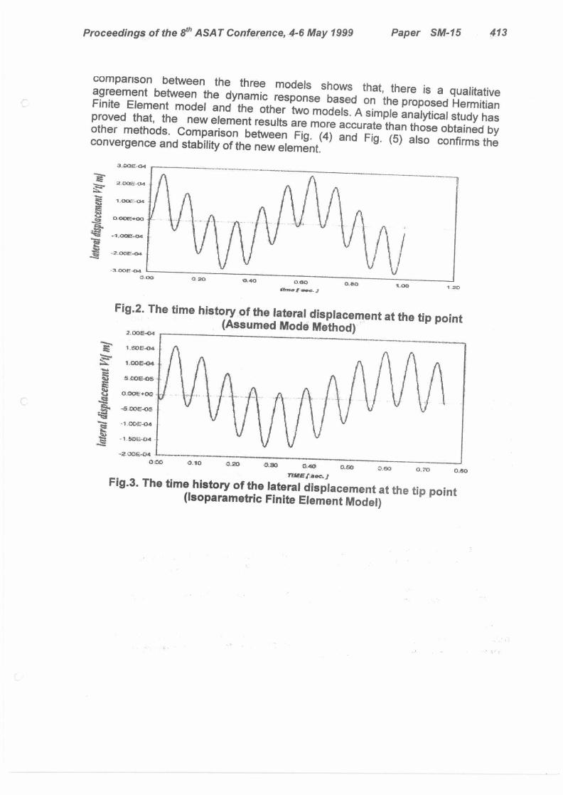
Fig.(2) and Fig.(3) show the time history of the displacement based on the assumed mode and the isoparametric finite element Fig.(4) shows the time history of the lateral displacement at the same conditions, based on the proposed Hermitian Finite Element two elements, and results with 4 Hermitian elements are shown

of the tip point method [3]. tip point, at the Method, using in Fig. (5).. The

3.00E.44

•04

1 04

0 20 0.40 040 114141. J

0.00 ac• 1 20 1.00

2.1)3Er.o4

i.exte-o4

1,00E-04

5.006.05

000t+00

-5.c0E-oe

-1 430E-04


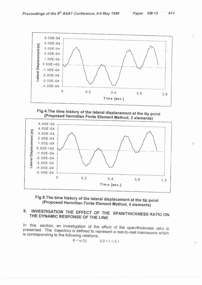
comparison between the three models shows that, there is a qualitative agreement between the dynamic response based on the proposed Hermitian Finite Element model and the other two models. A simple analytical study has proved that, the new element results are more accurate than those obtained by other methods. Comparison between Fig. (4) and Fig. (5) also confirms the convergence and stability of the new element.

Fig.2. The time history of the lateral displacement at the tip point (Assumed Mode Method)

000,-04 0.00 0.10 0,20 0.80 r3.40 0.50

MINE (see. J

Fig.3. The time history of the lateral displacement at the tip point (Isoparametric Finite Element Model)

0.60 0.70 0.50

Late

ral Dis

p lac

emen

t [m

] 5.00E-04 4.00E-04 3.00E-04

2.00E-04

1.00E-04 0.00E+00

-1.00E-04 -2.00E-04

-3.00E-04 -4.00E-04

0

0.2

0.4 0.6 Time [sec.]

0.8

Fig.4.The time history of the lateral displacement at the tip point (Proposed Hermitian Finite Element Method, 2 elements)

5.00E-04 4.00E-04 3.00E-04 2.00E-04 1.00E-04

0.00E+00 -1.00E-04 -2.00E-04 -3.00E-04 -4.00E-04 -5.00E-04

0 0.2 0.4 0.6 0.8 Time e [sec.]

Late

ral D

isp

lace

men

t


Paper SM-15 414

Fig.5.The time history of the lateral displacement at the tip point (Proposed Hermitian Finite Element Method, 4 elements)

9. INVESTIGATION THE EFFECT OF THE SPAN/THICKNESS RATIO ON THE DYNAMIC RESPONSE OF THE LINK

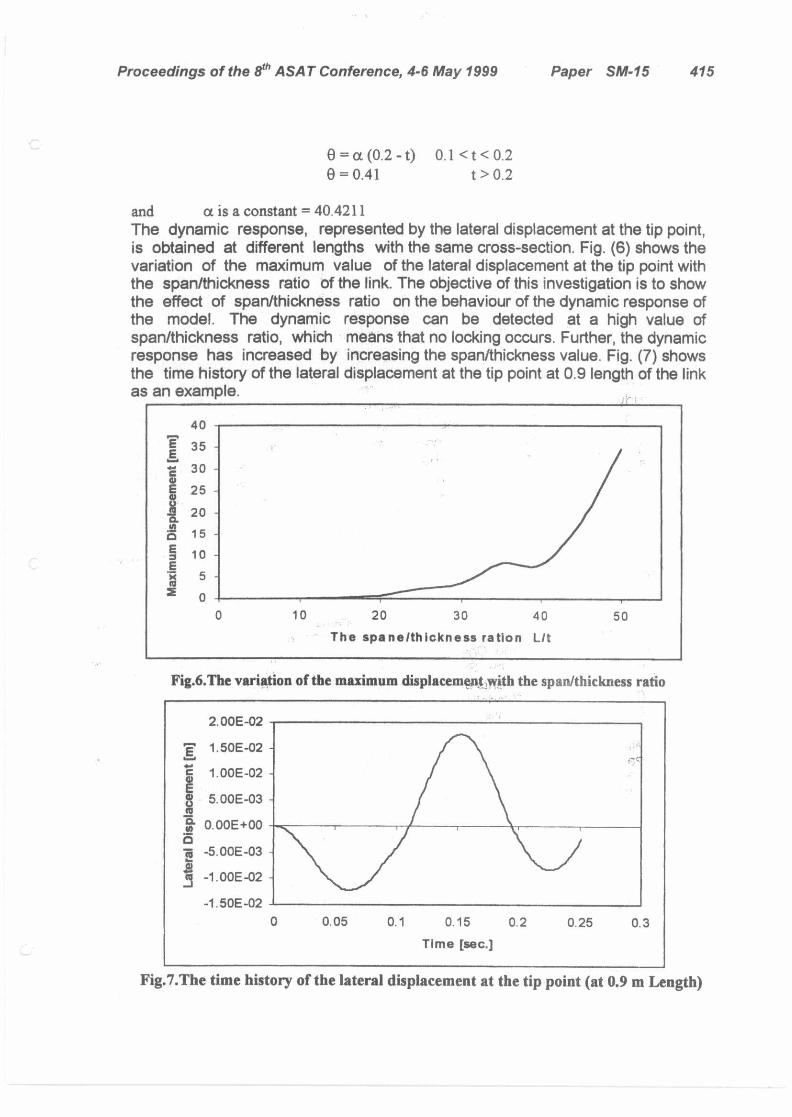
In this section, an investigation of the effect of the span/thickness ratio is presented. The trajectory is defined to represent a rest-to-rest manoeuvre which is corresponding to the following relations:

0 = a (t) 0.0 <t < 0.1

0 10 20 30 40 50

The spaneithickness ration Lit

40

35

30

25

20

15

10

5

0

E E

E

,u)

2

0 0.05 0.1 0.15

Time [sec.]

0.2 0.25 0.3

2.00E-02

1.50E-02 -

1.00E-02 -

5.00E-03 -

0.00E+00

-5.00E-03 -

-1.00E-02 -

-1.50E-02

Late

ral D

ispl

acem

e nt [

m]


0 =a(0.2-t)0.1<t< 0.2 0 =0.41 t> 0.2

and a is a constant = 40.4211 The dynamic response, represented by the lateral displacement at the tip point, is obtained at different lengths with the same cross-section. Fig. (6) shows the variation of the maximum value of the lateral displacement at the tip point with the span/thickness ratio of the link. The objective of this investigation is to show the effect of span/thickness ratio on the behaviour of the dynamic response of the model. The dynamic response can be detected at a high value of span/thickness ratio, which means that no locking occurs. Further, the dynamic response has increased by increasing the span/thickness value. Fig. (7) shows the time history of the lateral displacement at the tip point at 0.9 length of the link as an example.

Fig.6.The variation of the maximum displacemeAmith the span/thickness ratio

Fig.7.The time history of the lateral displacement at the tip point (at 0.9 m Length)

Proceedings of the 8Th ASAT Conference, 4-6 May 1999 Paper SM-15 416

10. CONCLUSIONS

A proposed dynamic model based on the Hermitian Finite Element Method and the Timoshenko beam theory has been presented. Shear deformation and rotary inertia effects are taken into consideration. The effect of flexibility on a beam is discussed and shows that it is very important factor when the beam is considered as flexible. Computer simulation program has been developed to solve this model. A derivation for the two-node Timoshenko beam element is introduced. The validity of the proposed model has been verified through the comparison between the dynamic response of a model based on assumed mode method [2] and another model is based on Isoparametric finite element method [5], and the proposed model. The comparison between the three models shows that, there is a qualitative agreement between the dynamic response based on the proposed Hermitian Finite Element model and the other two models. A simple analytical study has proved that, the new element results are more accurate than those obtained by other methods. Comparison between two and four elements response confirms also the convergence and stability of the new element. The presented method is better than the assumed mode method as the later is not suitable for non-regular cross-section. Finally, a case study has been investigated to show the effect of span/thickness ratio on the behaviour of the dynamic response of the model.

Acknowledgement: I gratefully acknowledge my M.Sc. supervisor Prof. A.S. Abdel Mohsen.

11. REFERENCES

[1] Book, W.J., "analysis of massless elastic chains with servo controlled joints", ASME J. of Dyn. Sys., Measurments and Control, Vol. 101, pp. 187-192, (1979).

[2] Petroka, R.P., and Chang, L.W., "Expermental validation of a dynamic model (Equivalent Rigid Link System) on a single-link flexible manipulator", ASME J. of Dyn. Sys., Measurments and Control, Vol.112, pp.138-143, (1990).

[3] Moutaz Hegaze, "Modeling and Control of Flexible Robot Manipulator", M.Sc. thesis, Military Technical College, Cairo, Egypt (1997).

[4] Parveen, K. and Anand, M.S., "Accurate modelling of flexible manipulators using finite element analysis" J. of Mech. Mach. Theory, Vol. 26, No.3, pp. 299- 313, (1991).

[5] AHMAD A. SMAILI, "A three-node finite beam element for dynamic analysis of planar manipulators with flexible joints" J. of Mech. Mach. Theory, Vol. 28, No.2, pp. 193-206, (1993).

[6] A EI-Zafrany and R A Cookson, "An improved N-node Timoshenko beam finite element", Applied Mechanics Group, SME, Cranfield University, (1986).

[7] Cowper, G.P., "The shear coefficient in Timoshenko's beam theory" J. of Applied Mechanics, Vol. 33, pp 335-340, (1966).

Proceedings of the 81h ASAT Conference, 4-6 May 1999 Paper SM-15 417

The element stiffness matrix IC

A. 0

APPENDIX

0 - A. 0 0 0 12 6L 0 -12 6L

= E I 0 6L 4L2 + 0 - 6L 2L2 - L (L2 + 0) -A. 0 0 A. 0 0

0 -12 - 6L 0 12 - 6L 0 6L 2L2 - f3 0 - 61 412 + 0_

With

A = E A L

The element mass matrix M*

12E1 p = 2 k2 G A

M* = Ma + Mbv + M + Mbu + M„

2 0 0 1 0 0- 0 0 0 0 0 0 0 0 0 0 0 0 0 156 22 L 0 54 -13 L

= pAL 0 0 0 0 0 0 Mbv = pAL 0 22L 4L2 0 13L -3L2 6 1 0 0 2 0 0 420 0 0 0 0 0 0

0 0 0 0 0 0 0 54 13 L 0 156 - 22 L 0 0 0 0 0 0 0 - 13 L -3L2 0 - 22 L

0 0 0 0 0 0 0 (-36 + 4q) (-11 + 2q)L 0 (36 - 4q) (-11 + 2q)L

pALq 0 (-11 + 2q)L (-2 + q)L2 0 (11 - 2q)L (-2 + q)L2 840 0 0 0 0 0 0

0 (36 - 4q) (11 - 2q)L 0 (-36 + 4q) (11 - 2q)L _0 (-11 + 2q)L (-2 + q)L2 0 (11 - 2q)L (-2 + q)L2


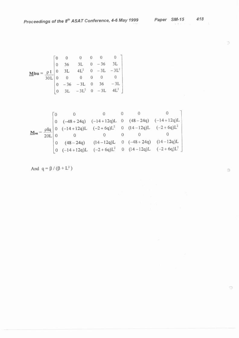
0 0 0 0 0 0 36 3L 0 - 36 3L

Mbu = P ' 0 3L 4 L2 0 3L -312 30L 0 0 0 0 0 0

0 - 36 3L 0 36 - 3L 0 3L - 3 L2 0 - 3L 4 L2

0 0 0 0 0

0 (-48+ 24q) (-14 +12q)L 0 (48 - 24q) (-14 +12q)L

0 (-14 +12q)L (-2 + 6q)L2 0 (14 -12q)L (-2 + 6q)L2 M Pig

-311 20L 0 0 0 0 0 0

0 (48 - 24q) (14 -12q)L 0 (-48 + 24q) (14 -12q)L

0 (-14 +12q)L (-2 + 6q)L2 0 (14 -12q)L (-2 + 6q)L2

And q =13 / ((3 +12 )

Documents

THE USE OF HERMITIAN TIMOSHENKO FINITE ELEMENT FOR …