Examensarbete vid Institutionen för geovetenskaper Degree Project at the Department of Earth Sciences

ISSN 1650-6553 Nr 322

The Usability of Remote Sensing Data for Flood Inundation Modelling: a Case

Study of the Mississippi River Användbarheten av fjärranalysdata för

översvämningsmodellering: en fallstudie av Mississippifloden, USA

Åsa Horgby

INSTITUTIONEN FÖR GEOVETENSKAPER

D E P A R T M E N T O F E A R T H S C I E N C E S

Examensarbete vid Institutionen för geovetenskaper Degree Project at the Department of Earth Sciences

ISSN 1650-6553 Nr 322

The Usability of Remote Sensing Data for Flood Inundation Modelling: a Case

Study of the Mississippi River Användbarheten av fjärranalysdata för

översvämningsmodellering: en fallstudie av Mississippifloden, USA

Åsa Horgby

ISSN 1650-6553 Copyright © Åsa Horgby and the Department of Earth Sciences, Uppsala University Published at Department of Earth Sciences, Uppsala University (www.geo.uu.se), Uppsala, 2015

Abstract The Usability of Remote Sensing Data for Flood Inundation Modelling: a Case Study of the Mississippi River Åsa Horgby The probability and impact of flooding is projected to increase in the future. This is due to climate and land-use changes (e.g. urbanization) in addition to the ongoing socioeconomic development of many floodplain areas. Exploiting the increasing availability of satellite data for flood inundation modelling will allow mapping floods in remote, data-poor areas to lower costs, and thereby make it possible to estimate flood risks in areas that today lack the economic resources needed for supporting risk assessment. In this context, this study has investigated the potentials and limitations of using low-cost, global remote sensing data (i.e. SRTM) to support flood inundation modelling. To this end, a case study of a river reach along the Mississippi was exploited. In particular, two flood inundation models were built by using the same 2D hydraulic model code (LISFLOOD-FP), but with two different topographical inputs, i.e. high quality/accuracy LiDAR topography data and the freely available SRTM topography data. The LiDAR data was lowered to the same resolution as the SRTM data and the two models were run with the resolution of 83x83 m2. Thereafter, the models were compared by simulating two historical flood events of different magnitude. The comparison of the two models showed that flood inundation modelling with satellite data is more accurate (closer to the reference model, i.e. LiDAR-based model) for the higher magnitude flood event than for the lower magnitude flood event. This was attributed to the relatively reduced importance of micro topography during bigger flood events. An area-based performance measure gave a value of the correspondence (i.e. the fit) between the predicted flood extents for the two models. The areas/pixels were reclassified in ARC GIS to flooded or dry. Thereafter, areas flooded in both the LiDAR and the SRTM simulations were divided by the sum of the areas flooded in both or in one of the simulations (LiDAR or SRTM). From this procedure the fit could be determined, where a fit of 100 % would mean that the simulations had predicted the same flood extents. For the high magnitude flood event simulated in this study, the fit in terms of flood extent between the LiDAR-based and the SRTM-based model was 72 %, while the fit for the smaller flood was only 38 %. In this study, model calibration was preformed manually because of limited availability of time and computational power. However, this is not considered a major limitation as the work does not aim to make a faultless model of this river reach of the Mississippi, but rather to determine the potentials and limitations of SRTM topography data in supporting flood inundation modelling. Additional studies of rivers systems with different properties, flood magnitudes, vegetation covers and river scales should be conducted, to further validate the usability of remote sensing data for flood inundation modelling. Keywords: Flood inundation modelling, LISFLOOD-FP, LiDAR, SRTM, remote sensing, hydrology Degree Project E1 in Earth Science, 1GV025, 30 credits Supervisor: Giuliano Di Baldassarre Department of Earth Sciences, Uppsala University, Villavägen 16, SE-752 36 Uppsala (www.geo.uu.se) ISSN 1650-6553, Examensarbete vid Institutionen för geovetenskaper, No. 322, 2015 The whole document is available at www.diva-portal.org

Populärvetenskaplig sammanfattning Användbarheten av fjärranalysdata för översvämningsmodellering: en fallstudie av Mississippifloden, USA Åsa Horgby Stora områden runt om i världen har problem med översvämningar, som står för 40 % av alla dödsfall orsakade av naturkatastrofer. Det är troligt att risken för översvämningar kommer att öka i framtiden på grund av klimatförändringar och ändrad landanvändning, som till exempel urbanisering. Ett problem är att det ofta är dyrt att göra kartor som beskriver översvämningsrisker och därför finns det många områden där kunskap om riskerna saknas. I denna studie har det undersökts huruvida det är möjligt att använda globala fjärranalysdata (data från satelliter) för översvämningsmodellering. Detta skulle möjliggöra framställandet av kartor över översvämningsrisker till en låg kostnad, och därmed nå ut till områden där idag inte finns ekonomiska resurser nog för detta. En fallstudie har gjorts av en sträcka utmed Mississippifloden (USA) och två översvämningsmodeller har byggts genom att använda samma hydrauliska modelleringskod (LISFLOOD-FP). Skillnaden mellan modellerna var att den ena modellen byggdes med hjälp av LiDAR-topografidata, medan den andra modellen baserades på gratis SRTM- topografidata. LiDAR-data är högkvalitativt och högupplöst data (1 meter upplösning) insamlat från flygplan med hjälp av laser. SRTM-data har endast 30-90 meters upplösning (83 meter inom fallstudie-området) och är insamlat av satelliter. Upplösningen av LiDAR-datat ändades till samma upplösning som för SRTM-datat och båda modellerna kördes med en upplösning av 83x83 m2. De två modellerna jämfördes genom att två historiska översvämningar, en liten år 2008 och en mycket stor år 1993, simu-lerades. Jämförelsen av de två modellerna visade på att modellering med hjälp av satellitdata är mer precist och närmare referensmodellen, det vill säga den LiDAR-baserade modellen, för större över-svämningar än för mindre översvämningar. Förklaringen till detta tillskrevs den relativt reducerade bety-delsen av mikrotopografi för större översvämningar. Överrensstämmelsen mellan modellresultaten räk-nades ut genom att områdena/pixlarna först blev omklassificerade i ARC GIS som översvämmande eller icke översvämmade. Därefter delades antalet områden som svämmades över i båda simuleringarna med antalet områden som svämmades över i båda simuleringarna eller i den ena av simuleringarna. På detta sett kunde en faktor för överensstämmande bestämmas, där en faktor på 100 % innebar att modellerna förutspådde lika stora översvämningar. För den större översvämningen som simulerades överensstämde, i fråga om utbredning, de två modellerna (LiDAR och SRTM) till 72 %, medan modellerna för den mindre översvämningen endast överensstämde till 38 %. I denna studie gjordes kalibreringen manuellt då den tillgängliga tiden och datorkapaciteten var begränsad. Dock så anses inte detta vara en stor begränsning eftersom studien inte syftade till att göra en felfri modell av översvämningsriskerna utmed en sträcka av Mississippifloden, utan till att undersöka användbarheten och begränsningarna av satellitdata för översvämningsmodellering. Denna studie stödjer tidigare teorier om att globala satellit-data har stort användningsområde för att simulera översvämningsrisker. Dock behövs fler studier av flodsystem med olika egenskaper, storlek på översvämningar och vegetation göras för att ytterligare validera detta. Nyckelord: Översvämningsmodellering, LISFLOOD-FP, LiDAR, SRTM, fjärranalys, hydrologi Examensarbete E1 i geovetenskap, 1GV025, 30 hp Handledare: Giuliano Di Baldassarre Institutionen för geovetenskaper, Uppsala universitet, Villavägen 16, 752 36 Uppsala (www.geo.uu.se) ISSN 1650-6553, Examensarbete vid Institutionen för geovetenskaper, Nr 322, 2015 Hela publikationen finns tillgänglig på www.diva-portal.org

Table of Contents

1. Introduction .......................................................................................................................... 1

2. Aim ......................................................................................................................................... 3

3. Background ........................................................................................................................... 4 3.1 Previous Research ............................................................................................................................... 4 3.2 Floodplain Inundation Models ............................................................................................................ 5 3.3 Development of LISFLOOD-FP ......................................................................................................... 6

3.3.1 Floodplain Flow Solvers ..................................................................................................... 7 3.3.2 Channel Flow Solvers ......................................................................................................... 8

3.4 Case Study Area: the Mississippi River .............................................................................................. 8

4. Methodology ....................................................................................................................... 13 4.1 Data Requirements ............................................................................................................................ 13 4.2 Model Calibration .............................................................................................................................. 13 4.3 Model Setup ...................................................................................................................................... 14

4.3.1 Parameter File ................................................................................................................... 14 4.3.2 Digital Elevation Model File ............................................................................................ 14 4.3.3 River File .......................................................................................................................... 15 4.3.4 Boundary Condition File .................................................................................................. 15 4.3.5 Stage File .......................................................................................................................... 15

4.4 Model Performance Assessment ....................................................................................................... 16

5. Results ................................................................................................................................. 17 5.1 DEM Evaluation ................................................................................................................................ 17 5.2 Results of Calibration ........................................................................................................................ 19 5.3 Stage Evaluation ................................................................................................................................ 21 5.4 Flood Inundation Dynamics .............................................................................................................. 23 5.5 Classification of Flooded Areas ........................................................................................................ 26

5.5.1 Fit of the 2008 Flood Event .............................................................................................. 26 5.5.2 Fit of the 1993 Flood Event .............................................................................................. 27 5.5.3 Comparison of the Flood Occasions ................................................................................. 28

6. Discussion ............................................................................................................................ 29

7. Conclusions ......................................................................................................................... 32

8. Acknowledgements ............................................................................................................. 33

9. References ........................................................................................................................... 34

Appendix A ............................................................................................................................. 38

Appendix B .............................................................................................................................. 39

Appendix C ............................................................................................................................. 42

1

1. Introduction Flooding is a worldwide issue as it accounts for 40 % of all deaths resulting from natural catastrophes,

especially in developing and tropical regions, where the number of affected people is extremely high

(Ohl and Tapsell, 2000). It is projected that the probability and impact of flooding might increase in the

future, due to climate change and changes in land-use, such as urbanization, and because of the

socioeconomic development of many floodplain areas around the world (Di Baldassarre et al., 2010).

The impact of flooding depends to a large extent on the socioeconomic and health conditions in the

affected area. In areas with low socioeconomic conditions the capacity for dealing with floods is less

and the food and water supplies, sanitation, communication and transportation may be disrupted, which

triggers outbreaks of diseases such as acute infections, diarrhea, measles and cholera (CDC, 1989).

Floodplain modelling is needed all over the world to build flood maps and make risk assessments, to

better cope with a flooding (Sanders, 2007). Population growth and economic development, together

with ungauged river systems, make flood risk assessment problematic. Floodplain mapping is needed

to make people living in floodplain areas aware of the risk and to discourage new settlements and

developments there (Padi et al., 2011). Further advancements of floodplain modelling and creation of

flood risk maps are not only needed in countries with low socioeconomic standards; it is needed all over

the world (Castellarin et al., 2011).

According to the United Nations International Strategy for Disaster Reduction (UNISDR), risk is

“the combination of the probability of an event and its negative consequences” (UNISDR, 2009). To

estimate the risk, the damage of an event (which is an integral of the probabilities of occurrence) is

multiplied by the consequences of the event (Winsemius et al., 2013). Flood risk assessment is made up

by three parts; risk analysis (hazard, vulnerability and risk determination), disaster mitigation (structural

and non-structural measures) and preparedness (planning disaster relief, early warning and evacuation)

(Plate, 2002). There are different strategies to reduce flood risk, and both structural and non-structural

flood protection measures can be taken. Structural measures are physical constructions, such as dams

and flood levees, while non-structural measures use knowledge, agreement or practice to reduce the risk.

Examples of this kind are land-use planning laws, education and flood forecast systems (UNISDR,

2009). All protection measures rely on flood predictions and therefore the accuracy of the predictions

affects the effectiveness of the protection measures significantly (Sanders, 2007). To design flood risk

maps the risk has to be identified, assessed, communicated and mitigated (FEMA, 2015). Identification

of the risk can be difficult in areas with low economic capacity, because it requires data of river

conditions and floodplain properties. Due to the increasing problem with floods, there is a higher

demand for flood risk maps. The question is, however, how those could be built in data-poor areas of

the world.

A possible method could be to take advantage of the growing availability of multi-temporal remote

sensing data. Satellite data offer effective ways to monitor floodplain inundation dynamics (Smith,

2

1997) and their growing availability leads to an increasing possibility to make regular observations of

river systems (Patro et al., 2009). The global in situ gauging networks of today are not capable of

supporting the process of flood risk mapping, and therefore remote sensing technologies can provide

vital knowledge of the dynamics of surface water and offer a measuring tool for surface water area,

slope, elevation and temporal change (Alsdorf et al., 2007). Considering the increasing availability and

precision of remote sensing data, there are also more and more possibilities of measuring water stages

and discharge from space (Smith, 1997). Thus, when monitoring big and complex floodplains, previous

studies have shown that remote sensing data can contribute with plentiful of important information (Jung

et al., 2011) to improve the flood risk assessment in data-poor areas of the world (Di Baldassarre et al.,

2011). In situ gauging networks are then complemented with remote sensing systems, which improves

the model output (Patro et al., 2009).

There are different sources of topography data that can be used to create the digital elevation models

(DEMs) used as input of floodplain inundation models. Using highly accurate and costly topographic

data is not always possible due to time and budget limitations. A low-cost approach would consist of

building flood inundation models by using a global DEM, from satellites, such as the free Shuttle Radar

Topography Mission data (SRTM), instead of the more expensive Light Detection and Ranging data

(LiDAR) that has to be collected by an aircraft. SRTM topography data has a relatively high height error

(from 5 to 10 meters (Rodríguez et al., 2006); but much lower in floodplains; see e.g. Yan et al., 2015)

and low horizontal resolution (30-90 meters) (Sanders, 2007). The measuring mission took place on

February 11-21 in 2000, onboard the Space Shuttle endeavor. During ten days 80 % of the Earth’s

topography was measured with radar to later on be put freely available online (Farr and Kobrick, 2000).

LiDAR data has a much higher precision with a vertical accuracy of 0.05-0.2 meters and a horizontal

resolution of about 1-3 meters. The LiDAR technology was developed in 1994 and the topography data

is collected by a laser scanner from an aircraft or helicopter. A Global Positioning System (GPS)

measures the sensor position and an Inertial Measurement Unit (IMU) provides the orientation. The

laser creates pulses of light that are directed at the Earth’s surface and reflected back to the aircraft.

LiDAR gives highly accurate data but to a high cost (Smith et al., 2006).

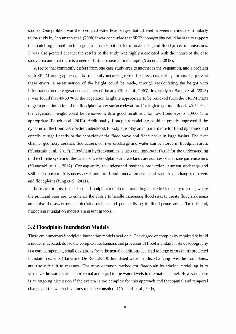
There is an ongoing discussion on the potentials and limitations of these free low-resolution data

with reference to their appropriateness in supporting flood inundation modelling. Previous studies have

shown that they have some potential to be useful, but more studies are needed (Yan et al., 2013). The

hypothesis tested in this study is whether using SRTM data to support flood inundation modelling can

provide reasonably accurate results. If this could be validated, it would increase the possibilities of

creating flood risk maps in data-poor areas and contribute to improve flood risk assessment all over the

world.

3

2. Aim The aim of this master thesis is to investigate whether low-cost, global remote sensing data can be used

with reliable results for flood inundation modelling. A case study of a river reach along the Mississippi

(USA) is investigated by comparing two flood inundation models: one based on LiDAR data and a

second one based on SRTM data. This is expected to give insights on the usefulness and limitations of

remote sensing data for floodplain inundation modelling.

4

3. Background To simulate floodplain inundation dynamics, during different hydrological conditions, hydraulic

modelling is needed. These models are only simplifications of the reality and always contain

uncertainties and errors, which have to be considered. In this section, previous research of the usability

of remote sensing data for flood inundation modelling is described, the necessary modelling parameters

identified and the potential errors emphasized. The differences between several floodplain inundation

models are explained and the model code chosen in this study, LISFLOOD-PF, is described. Last in this

section, an overview of the case study area is presented.

3.1 Previous Research The topic of flood inundation modelling with remote sensing data has been widely debated over the last

years, and many studies indicate that there are very high potentials of satellite data to support

hydrological models (for example studies by Yan et al. 2013; Smith 1997; Patro et al. 2009; Alsdorf et

al. 2007; Di Baldassarre et al. 2011; Jung et al. 2011). The increasing availability of remote sensing

topography data together with increasing computation power, have created a possibility to do flood

inundation modelling to a decreased data cost and computational time (Dottori and Todini, 2011; Di

Baldassarre et al., 2011), and there are extensive potentials for furthering progress of the usage of the

remote sensing tools (Alsdorf et al., 2007). However, there are still plentiful of uncertainties and

limitations connected to this and the topic has to be further investigated (Di Baldassarre et al., 2011).

The core of some environmental models is the DEM used (Schumann et al., 2008), which contains

many uncertainties that have to be considered, such as for example potential errors propagating through

the modelling and grid cell resolution (Wechsler, 2007). Due to the importance of the DEM, these

uncertainties have to be taken into consideration.

A variety of studies of the usability and validity of DEMs based on remotely sensed data has been

made. One study, conducted by Schumann et al. (2008) compared water stages derived from LiDAR

data with water stages derived from topography contours and from SRTM data. A flood inundation

model calibrated with high water marks was used. It was concluded that the SRTM model preformed

unexpectedly accurate results when it was compared with the LiDAR model and the contour model. The

good performance was linked to the low-lying floodplain. In the study it was concluded that SRTM

models can be used to give initial information of floods in large and homogenous floodplains (Schumann

et al., 2008). Another comparative study on the value of SRTM topography data to support flood

inundation modelling was a case study of the Po River conducted by Yan et al. (2013). The 1D model

HEC-RAS was used and a hydrologic model based on profiles derived from LiDAR topography data

was compared to a model based profiles derived from SRTM topography data. The results of the study

showed that there were significant differences between the two model outcomes, but that the accuracy

of the SRTM model was still acceptable and within the range that is associated with large-scale flood

5

studies. One problem was the predicted water level stages that differed between the models. Similarly

to the study by Schumann et al. (2008) it was concluded that SRTM topography could be used to support

the modelling in medium to large-scale rivers, but not for ultimate design of flood protection measures.

It was also pointed out that the results of the study was highly associated with the nature of the case

study area and that there is a need of further research in the topic (Yan et al., 2013).

A factor that commonly differs from one case study area to another is the vegetation, and a problem

with SRTM topographic data is frequently occurring errors for areas covered by forests. To prevent

these errors, a re-estimation of the height could be made, through recalculating the height with

information on the vegetation structures of the area (Sun et al., 2003). In a study by Baugh et al. (2013)

it was found that 40-60 % of the vegetation height is appropriate to be removed from the SRTM DEM

to get a good imitation of the floodplain water surface elevation. For high magnitude floods 40-70 % of

the vegetation height could be removed with a good result and for low flood events 50-80 % is

appropriate (Baugh et al., 2013). Additionally, floodplain modelling could be greatly improved if the

dynamic of the flood were better understood. Floodplains play an important role for flood dynamics and

contribute significantly to the behavior of the flood wave and flood peaks in large basins. The river

channel geometry controls fluctuations of river discharge and water can be stored in floodplain areas

(Yamazaki et al., 2011). Floodplain hydrodynamics is also one important factor for the understanding

of the climate system of the Earth, since floodplains and wetlands are sources of methane gas emissions

(Yamazaki et al., 2012). Consequently, to understand methane production, nutrient exchange and

sediment transport, it is necessary to monitor flood inundation areas and water level changes of rivers

and floodplains (Jung et al., 2011).

In respect to this, it is clear that floodplain inundation modelling is needed for many reasons, where

the principal ones are: to enhance the ability to handle increasing flood risk; to create flood risk maps

and raise the awareness of decision-makers and people living in flood-prone areas. To this end,

floodplain inundation models are essential tools.

3.2 Floodplain Inundation Models There are numerous floodplain inundation models available. The degree of complexity required to build

a model is debated, due to the complex mechanisms and processes of flood inundation. Since topography

is a core component, small deviations from the actual conditions can lead to large errors in the predicted

inundation extents (Bates and De Roo, 2000). Inundated water depths, changing over the floodplains,

are also difficult to measure. The most common method for floodplain inundation modelling is to

visualize the water surface horizontal and equal to the water levels in the main channel. However, there

is an ongoing discussion if the system is too complex for this approach and that spatial and temporal

changes of the water elevations must be considered (Alsdorf et al., 2005).

6

Thus, what exact parameters and processes that actually need to be included in floodplain inundation

models are still today debated (Bates and De Roo, 2000) and there are many uncertainties associated to

it (for example model structure, model parameters, boundary conditions and topography data) (Yan et

al., 2013). A common rule is to keep the model that is as simple as possible (“parsimony principle”).

Popular 1D flood inundation models, such as MIKE-11 and HEC-RAS, use the full St. Venant equations,

and a series of cross-sections, to describe the river channel and the floodplains. The velocity and water

depth are calculated for each cross-section and defining the shape of the cross-section is therefore very

important and a big source of potential errors. Interpolation between the cross-sections is another

potential source of error, when the areas between the cross-sections are not well represented. To

overcome the problems with the 1D models, a number of 2D models have been developed. The

topography is then more continuously represented and the river hydraulic processes better characterized.

Those models has been proven to be successful but they are more costly in respect to computational

power (Bates and De Roo, 2000).

There are no consensus or general guidelines concerning which model to select when conducting a

study. According to Castellarin et al. (2011), the choice depends on the available data, the accuracy of

topography data and the calibration of the data. Many comparative studies of 1D, quasi-2D and 2D

inundation models have been made, and 1D and quasi-2D are often able to perform as accurate

predictions as the 2D models. However, when it comes to complex topographies or urban floodplain

areas, the 2D models have been found to predict more accurate results (Castellarin et al., 2011).

3.3 Development of LISFLOOD-FP The ongoing development of flood inundation models is linked to the development of floodplain DEMs

with higher resolution and accuracy. Researchers at the University of Bristol have developed a 2D raster

based flood inundation modelling code, LISFLOOD-FP, which is a further development of the

LISFLOOD catchment model. The LISFLOOD-FP model has been proven in some studies to be very

useful but the uncertainty has to be considered. There is a need for more work to further validate the

model; through investigate floods of different magnitudes and the impact of topography (Bates and De

Roo, 2000).

Building a model with the LISFLOOD-FP modelling code requires a DEM of the channel and

floodplain, defined boundary conditions for the inflow and the outflow of the domain, and flood

hydraulic data such as discharge hydrographs from gauging stations, water stage records and images of

flood extents (Bates and De Roo, 2000). Simplifications of shallow water equations are used to describe

the water propagation. Below the momentum equation (1) for the 1D full shallow water equations is

expressed, describing that the sum of local acceleration, convective acceleration, water slope and friction

slope is equal to zero (Bates et al., 2013). Then the continuity equation (2) for the 1D full shallow water

equations is described.

7

0 = 𝜕𝜕𝑄𝑄𝑄𝑄𝜕𝜕𝑡𝑡

+ 𝜕𝜕𝜕𝜕𝑄𝑄�𝑄𝑄𝑄𝑄

2

𝐴𝐴� + 𝑔𝑔𝑔𝑔 𝜕𝜕 (ℎ+𝑧𝑧)

𝜕𝜕𝑄𝑄+ 𝑔𝑔𝑔𝑔2𝑄𝑄𝑄𝑄2

𝑅𝑅4/3𝐴𝐴 (1)

0 = 𝜕𝜕𝐴𝐴𝜕𝜕𝑄𝑄

+ 𝜕𝜕𝑄𝑄𝑄𝑄𝜕𝜕𝑄𝑄

(2)

Equation 1 and Equation 2. In the equations, Qx is volumetric flow rate in the x Cartesian direction; A is the cross-sectional area of the flow; h is water depth; z is bed elevation; g is gravity; n is Manning’s coefficient; R is hydraulic radius; t is time and x is the distance in the x Cartesian direction.

The properties of the modelling code are described in the LISFLOOD-FP user manual (code release

5.9.6) by Bates et al. (2013). In LISFLOOD-FP the propagation of flood waves along channels and

floodplains is simulated by numerical solvers and depends on the characteristics of the modelled system

and the data available. The purpose of the solvers is to calculate the amount of water that flows between

adjacent cells over a given time, and for each node at each time-step the water depth and the velocity is

computed. There are two types of solvers; for floodplain flow and for channel flow (Bates et al., 2013).

3.3.1 Floodplain Flow Solvers There are five floodplain flow solvers; the routing solver, the flow-limited solver, the adaptive solver,

the acceleration solver and the roe solver. The difference between them is the dimensions (commonly

1D on 2D grid), which shallow water terms that are included and which that are assumed to be negligible

and how the time step is defined (Bates et al., 2013).

The routing solver assumes all shallow water terms negligible and water flows from higher elevated

cells to lower elevated cells, where the flow direction is pre-calculated. The flow limited solver is the

least complex solver using the shallow water equations, where the terms included are friction and water

slopes. Local and convective acceleration are assumed negligible. The time step is user determined

which creates a risk of cell emptying, where the cells can be completely drained during one time step

and thereby change the flow direction during the next time step. The adaptive solver has a varying time

step during the simulation, which overcome the potential problem of cell emptying. Thus, this may

extensively increase the simulation time. The acceleration solver assumes only the convective

acceleration negligible. The time step varies and is related to water depths and cell size, which may

decrease the computational time. The last floodplain flow solver, the roe solver, solves the full shallow

water equations (all terms are included). Though, the roe solver is very newly developed and needs to

be tested more before being commonly used (Bates et al., 2013).

8

3.3.2 Channel Flow Solvers Solvers available for calculating channel flow are the kinematic solver, the diffuse solver and the sub-

grid channel solver. All channel flow solvers calculate a 1D water flow. Similarly to the floodplain

solvers the channel solvers differ in terms of which shallow water terms that are included and which

that are assumed negligible. The time steps for the kinematic and diffusive solvers are linked to the used

2D floodplain solver or fixed, while the sub-grid channel solver uses an adaptive time step. The most

simple is the kinematic solver, where all terms, except the bed gradient and the friction, are assumed

negligible. The diffusive solver is able to predict backwater effects, due to the use of the 1D diffusive

wave equation (where the water slope term is included). The sub-grid channel solver is newly developed,

where the channel is divided into segments and water flow between the segments is calculated using

acceleration model equations. This solver is designed to be used for large areas with limited data

available (Bates et al., 2013).

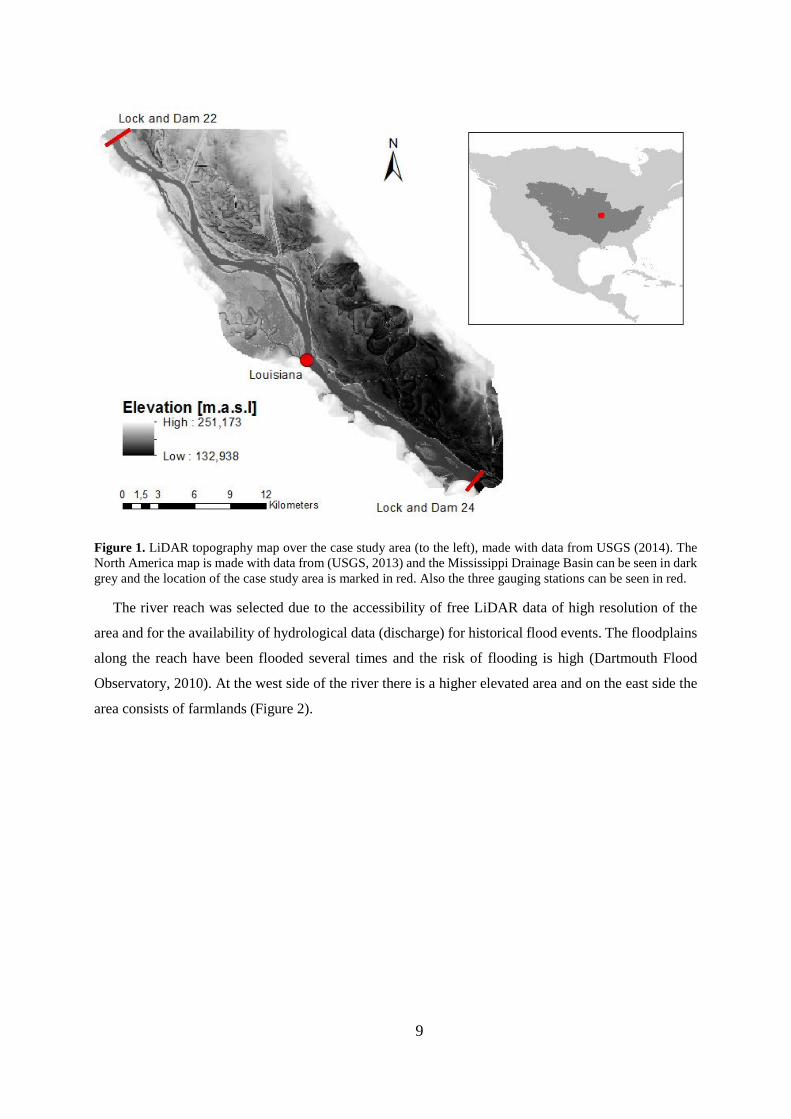
3.4 Case Study Area: the Mississippi River A river reach along the Mississippi in USA was selected as case study. The whole Mississippi River is

about 2010 kilometers long (UMESC, 2014). The drainage basin covers more than 3.200.000 square

kilometers and is the third largest drainage basin in the world (U.S. Army Corps of Engineers, 2015a).

The area surrounding the Mississippi River is highly populated and more than 30 million people depend

on the water from the river (for water supplies, nuclear power plant cooling and wastewater assimilation)

(UMESC, 2014). The chosen case study area reach along the river is called Navigation Pool 24 and is

situated south of the city Keokuk and north of St. Louis (Figure 1). The case study area is at the border

between Missouri to the west and Illinois to the east and the river reach is approximately 40 kilometers

long and the width varies from 300 meters to 4500 meters. The upstream and downstream boundaries

to the river reach are defined by two dams with gauging stations; Lock and Dam 22 in the north and

Lock and Dam 24 in the south. There is also a gauging station situated in the middle of the reach, close

to the village Louisiana (USGS, 2014).

9

Figure 1. LiDAR topography map over the case study area (to the left), made with data from USGS (2014). The North America map is made with data from (USGS, 2013) and the Mississippi Drainage Basin can be seen in dark grey and the location of the case study area is marked in red. Also the three gauging stations can be seen in red.

The river reach was selected due to the accessibility of free LiDAR data of high resolution of the

area and for the availability of hydrological data (discharge) for historical flood events. The floodplains

along the reach have been flooded several times and the risk of flooding is high (Dartmouth Flood

Observatory, 2010). At the west side of the river there is a higher elevated area and on the east side the

area consists of farmlands (Figure 2).

10

Figure 2. Satellite picture of the floodplain area from Google Earth (2014).

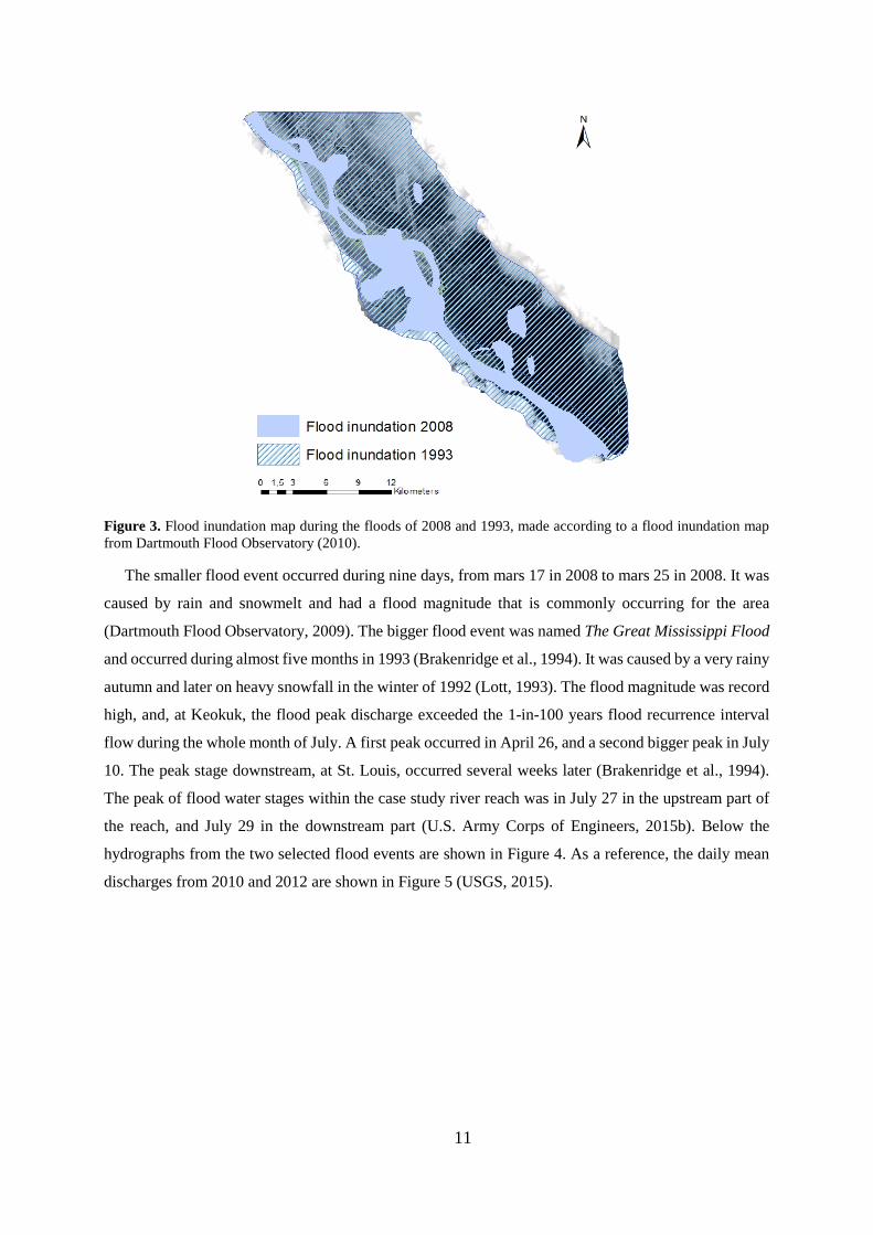
Two floods with different magnitudes were to be simulated, chosen due to different magnitudes and

extends, and because of the availability of flood inundation maps from the Dartmouth Flood Observatory

for those two floods. Figure 3 is a flood inundation map for the case study area, a zoomed modification

of a large scale flood inundation map from the Dartmouth Flood Observatory. It can be seen that the

flood of 2008 was only spreading over the area next to the Mississippi River main channel, while the

whole floodplain was inundated during the great flood of 1993. The flood inundation map was used for

calibration, where the parameters were calibrated so that the LiDAR-based model of the 2008 flood

would match the observed flood extent.

11

Figure 3. Flood inundation map during the floods of 2008 and 1993, made according to a flood inundation map from Dartmouth Flood Observatory (2010).

The smaller flood event occurred during nine days, from mars 17 in 2008 to mars 25 in 2008. It was

caused by rain and snowmelt and had a flood magnitude that is commonly occurring for the area

(Dartmouth Flood Observatory, 2009). The bigger flood event was named The Great Mississippi Flood

and occurred during almost five months in 1993 (Brakenridge et al., 1994). It was caused by a very rainy

autumn and later on heavy snowfall in the winter of 1992 (Lott, 1993). The flood magnitude was record

high, and, at Keokuk, the flood peak discharge exceeded the 1-in-100 years flood recurrence interval

flow during the whole month of July. A first peak occurred in April 26, and a second bigger peak in July

10. The peak stage downstream, at St. Louis, occurred several weeks later (Brakenridge et al., 1994).

The peak of flood water stages within the case study river reach was in July 27 in the upstream part of

the reach, and July 29 in the downstream part (U.S. Army Corps of Engineers, 2015b). Below the

hydrographs from the two selected flood events are shown in Figure 4. As a reference, the daily mean

discharges from 2010 and 2012 are shown in Figure 5 (USGS, 2015).

12

Figure 4. Hydrographs for the upstream gauging station Keokuk during the two flood events (USGS, 2015).

Figure 5. Hydrographs for the upstream gauging station Keokuk during normal flow conditions (USGS, 2015).

0

3000

6000

9000

12000

2008-03-17 2008-03-21 2008-03-25

m3/s

Date

Keokuk 2008

Discharge

0

3000

6000

9000

12000

1993-03-01 1993-05-31 1993-08-30

m3/s

Date

Keokuk 1993

Discharge

0

3000

6000

9000

12000

m3/s

Date

Daily mean discharge at Keokuk

Discharge 2012

Discharge 2010

13

4. Methodology To investigate the limitations and the potential of low-cost, global remote sensing data for flood

inundation modelling, the previous described modelling code LISFLOOD-FP was used. Two models

were built for the case study area: model A based on LiDAR topography data (reference model); and

model B based on SRTM topography data (testing model). For both models, two flood events were

simulated: the small flood of 2008 and the big flood of 1993. This was to test the impact of DEM

topography differences in flood inundation extents for different flood magnitudes. In this section, the

required data for the models, the calibration and model set up are described. Furthermore, the model

validation method is presented.

4.1 Data Requirements The data required for the models were: raster DEMs, inflow discharge hydrographs, channel slopes,

width and bankfull depths, initial estimates of channel flow depth, model time steps and Manning’s

roughness coefficients for the channel and floodplain friction (Bates and De Roo, 2000). Those data

were all found free of cost. The LiDAR topography data was provided by United States Geological

Survey (USGS). It was collected by airplane and firstly processed by The Upper Midwest Environmental

Sciences Center, and secondly by the U.S. Army Corps of Engineers Environmental Management

Program (EMP) and the Long Term Resource Monitoring Program (LTRMP) (USGS, 2014). The

SRTM topography data was from the CGIAR International Research Centers (CGIAR-CSI, 2004).

Channel slope, width and bankfull depth were derived from the DEMs and the initial estimate of channel

depth was assumed to be the same along the whole reach. Some of the data had to be modified in ARC

GIS and transformed into the required file formats while others had to be calculated in Excel.

4.2 Model Calibration As mentioned before, the parameters were calibrated so that the LiDAR-based model of the 2008 flood

would match the observed flood extent (Figure 3). Limited amount of water stage data was available,

and it was not enough to enable calibration of the model according to it. During the calibration process,

the channel depth and the Manning’s roughness coefficient of the main channel and floodplain were

modified, a common method for manual calibration of flood inundation models (Straatsma and Huthoff,

2011). The performances of different depths were tested, from 2 meters to 4 meters, and also different

channel geometries (rectangular geometry with the same depth along the reach and varying river

geometry where the depths were changing along the reach). Moreover, different Manning’s coefficient

values were assessed. Because of limited time and computational power, the calibration was performed

manually and a statistical calibration could not be made.

14

4.3 Model Setup To run a model using the LISFLOOD-FP modelling code, several input files had to be created; a

parameter file; digital elevation model file; river file boundary condition file and stage output file, see

appendix C for further information. The complete procedure of how to create the input files is explained

in the LISFLOOD-FP user manual (code release 5.9.6) by Bates et al. (2013). Below a short explanation

of the file characters and the set up in this study are described.

4.3.1 Parameter File The parameter file provides information that is necessary to run the simulation and it contains keywords

for file names, locations and run control parameters. Here, the names of the DEM file, river file,

boundary condition file and stage file were defined. Furthermore, the root for naming result files

(resroot), the directions of where the result files should be saved (dirroot), the saving interval (saveint),

the interval for the mass file to be written to (massint), the total length of the simulation (sim_time), the

initial guess for optimal time-step (initial_tstep) and the Manning’s coefficient for the floodplain (fpfric)

were defined.

The initial time step was chosen to be 30 seconds for both the 2008 flood simulation and the 1993

flood simulation. For 2008 flood simulation the mass interval was put to 3600 seconds (1 hour) and the

save interval to 72000 seconds (20 hours). Due to simulation time limits those parameter values were

set to 86400 seconds (1 day) respectively 172800 seconds (2 days) for the 1993 flood.

The choice for the channel flow solver was the diffuse solver, which uses a 1D diffusive wave

equation that, as mentioned before, includes water slope term (to deal with backwater effects) and

friction slope but is neglecting the local and convective acceleration (Bates et al., 2013). Because of the

diffuse solver, the keyword diffusive was put into the parameter file. The flow-limited floodplain solver

was chosen (where the time-step has to be defined) because due to time limits the adaptive or the

acceleration solvers could not be used. Therefore the keyword adapotoff was defined. Also elevoff were

put in to suppress the production of water surface elevation files.

4.3.2 Digital Elevation Model File The digital elevation model file gives information of the topography. The LiDAR topography data

consisted of 11 datasets that had to be merged together (using the mosaic tool in ARC GIS). The SRTM

topography data had to be clipped from a large DEM of the whole North America.

To enable comparison of inundated areas and evaluate the usability of the SRTM DEM, the pixel

resolution of the 1x1 m2 LiDAR DEM had to be reduced to the same resolution as the SRTM DEM,

which in this case was 83x83 m2 (appendix A). This was performed in ARC GIS by using the aggregate

tool, selecting a rescaling factor of 83 and using median value. The median was selected to avoid

influence of outliers. The SRTM DEM was resampled using bilinear interpolation, to match the LiDAR

15

DEM cell size. The DEMs had to have the same resolution because the LiDAR model was used as a

reference model, and the SRTM model tested against it. Lowering the resolution of the LiDAR DEM

enabled evaluation of the errors in the SRTM data, instead of focusing on limitations caused by the

lower resolution of the remote sensing data. If time and computational power would have been larger,

it could have been useful to test the LiDAR model with 1x1 m2 resolution too, but in this study it was

not achievable. Moreover, the coordinate systems of the DEMs had to correspond, and therefore the

SRTM DEM was re-projected from the geographic coordinate system WGS 1984 to the projected

coordinate system NAD 1983 UTM Zone 15 N (the coordinate system of the LiDAR DEM). Then the

two raster DEMs had to be converted to the esri ASCII file format to make simulations with the

LISFLOOD-FP modelling code possible.

4.3.3 River File The river file is the channel information file. In ARC GIS a vector of the river channel center line was

generated in the same coordinate system used for the DEMs (NAD 1983 UTM Zone 15 N). At 42 points

distributed along the river reach center line, the x- and y-coordinates, elevation (z-coordinate) and width

were measured for the LiDAR DEM respectively the SRTM DEM. In Excel the values were put into a

table where the different depths used for calibration were subtracted from the river bed elevations

derived from the DEMs. In this way the river files for the LiDAR model and the SRTM model were

created separately.

4.3.4 Boundary Condition File The days chosen to be simulated were two days before the floods begun (“warming up period”) to just

after the peak of the floods. The hydrographs from Keokuk during the two floods were set as inflow

discharge values. The upstream boundary condition was defined in the river file as QVAR (time varying

flow into domain) and the downstream as FREE (uniform flow). The average slope of the river reach

was calculated to 0.000073 meters, derived from the LiDAR DEM.

4.3.5 Stage File Although incomplete data of observed water stages a stage file was created to enable comparison of the

simulated river surface stages with observed stages during flood occurrences. The coordinates for the

simulated stages were put in to be the same as the three gauging stations along the river reach; Lock and

Dam 22, Louisiana station and Lock & Dam 24.

16

4.4 Model Performance Assessment To estimate the usefulness and the limitations of SRTM data for floodplain modelling, the SRTM-based

model was tested versus the LiDAR-based model. A number of operations were made in ARC GIS. The

height differences of the LiDAR and SRTM DEMs were evaluated. The root mean square error (RMSE),

which is a method to evaluate average model performance error, was calculated to get a value of the

mean absolute difference. First the differences between the LiDAR and SRTM DEMs were squared,

and then the root was taken from mean of the outcome (Willmott and Matsuura, 2005). Furthermore a

cross-section profile was made to investigate height differences between the LiDAR and SRTM DEMs

from the left river bank to the right river bank.

In ARC GIS the cells were also classified as dry or flooded, where cells with water depths less than

10 cm (the vertical accuracy of the LiDAR DEM) were classified as dry, and cells with water depths

exceeding 10 cm were classified as flooded. The classification was done separately for the LiDAR

simulation and for the SRTM simulation, but the same threshold of 10 cm was used. Thereafter the two

outcomes were added together, and the four different combinations of dry and flooded areas for the two

different flood events (2008 and 1993) were created. In a contingency table the numbers of the four

different combinations of cells dry or flooded was counted and added, and this area-based performance

measure gave a value of the correspondence, i.e. the fit, between the LiDAR and SRTM simulations

(Mason et al., 2011). As can be seen in Table 1, flooded areas in the LiDAR simulations got the value

1 and dry areas got the value 0, while flooded areas in the SRTM simulation got the value 5 and dry

areas 3. Then the reclassified LiDAR and the SRTM DEMs were added together, four areas (3-6) were

created and thereafter renamed to A-D.

Table 1. Using the raster calculator, the LiDAR simulation and the SRTM simulation were added together and the new fields received a letter (A-D).

Contingency table LiDAR flooded (1) LiDAR dry (0)

SRTM flooded (5) 6 = A 5 = B

SRTM dry (3) 4 = C 3 = D

The fit of the simulations based on SRTM data and on LiDAR data (the reference model), for the

two flood events, was calculated. A fit of 100 % would mean that the areas coincide, and the predicted

simulation totally corresponds to the observed inundation (Bates and De Roo, 2000).

𝐹𝐹 = #A#A + #B + #C

(3)

Equation 3. According to the formula, the fit is the sum of the intersecting flooded area divided by all

simulated areas (Stephens et al., 2012).

17

5. Results In the results section, the model based on SRTM topography data is compared with the model based on

LiDAR topography data. First, the differences of the DEMs are evaluated. Then the results of the effects

of the topography differences are presented; as water stage differences and flood inundation extent

differences.

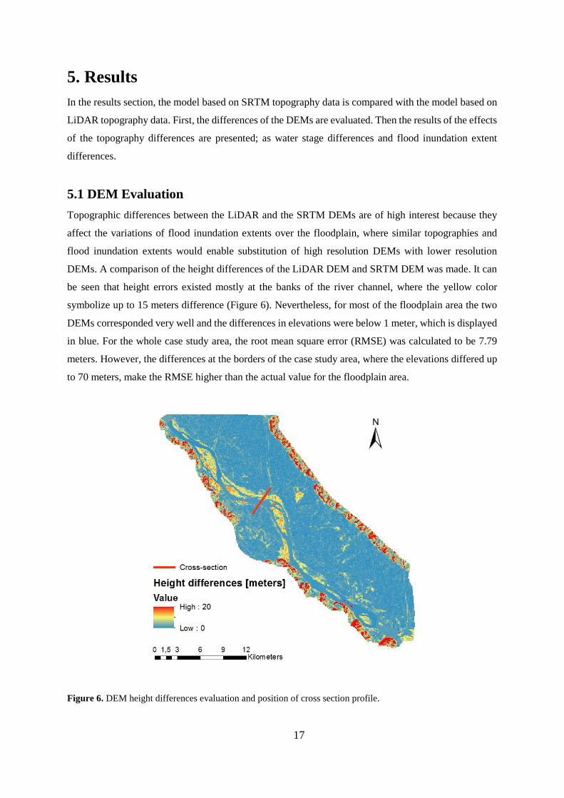
5.1 DEM Evaluation Topographic differences between the LiDAR and the SRTM DEMs are of high interest because they

affect the variations of flood inundation extents over the floodplain, where similar topographies and

flood inundation extents would enable substitution of high resolution DEMs with lower resolution

DEMs. A comparison of the height differences of the LiDAR DEM and SRTM DEM was made. It can

be seen that height errors existed mostly at the banks of the river channel, where the yellow color

symbolize up to 15 meters difference (Figure 6). Nevertheless, for most of the floodplain area the two

DEMs corresponded very well and the differences in elevations were below 1 meter, which is displayed

in blue. For the whole case study area, the root mean square error (RMSE) was calculated to be 7.79

meters. However, the differences at the borders of the case study area, where the elevations differed up

to 70 meters, make the RMSE higher than the actual value for the floodplain area.

Figure 6. DEM height differences evaluation and position of cross section profile.

18

To further evaluate the differences in the DEMs, a cross section was put in the middle of the reach,

starting from the west side of the river channel and ending at the eastern bank. Also here are the errors

concentrated generally just at the sides of the river channel. In the cross-section profile there is a first

small peak at 1400 meters distance along the profile where the western river bank is situated (displayed

in yellow in Figure 6). Then, at the location of the river channel, the height differences are small (1

meter) to increase extensively at the eastern border of the channel, where the differences go up to 13

meters. Moreover, Figure 7 shows the topographic errors that can arise in using a SRTM DEM.

Figure 7. Profile along the cross section, the LiDAR DEM profile shown as a solid line and the SRTM DEM as a dashed line.

In Figure 8 it can be seen that the LiDAR bed elevation surface is smoother than for the SRTM DEM,

and it can also be seen that the river surface elevation was higher in the LiDAR DEM than in the SRTM

DEM. The river surface elevation drops in the beginning and the end of the river reach, which can be

explained by the dams situated there, controlling the water flow. The SRTM DEM has higher elevated

river banks, but lower elevated river channel, which would make a flooding more difficult.

134

136

138

140

142

144

146

148

150

152

154

0 1000 2000 3000 4000 5000

Hei

ght (

met

ers)

Distance along cross section (meters)

Cross section

LiDAR

SRTMRiver channel

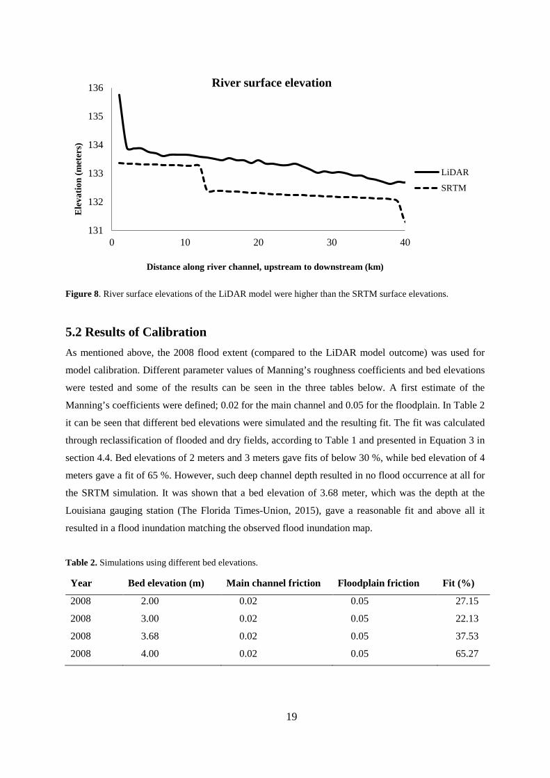
19

Figure 8. River surface elevations of the LiDAR model were higher than the SRTM surface elevations.

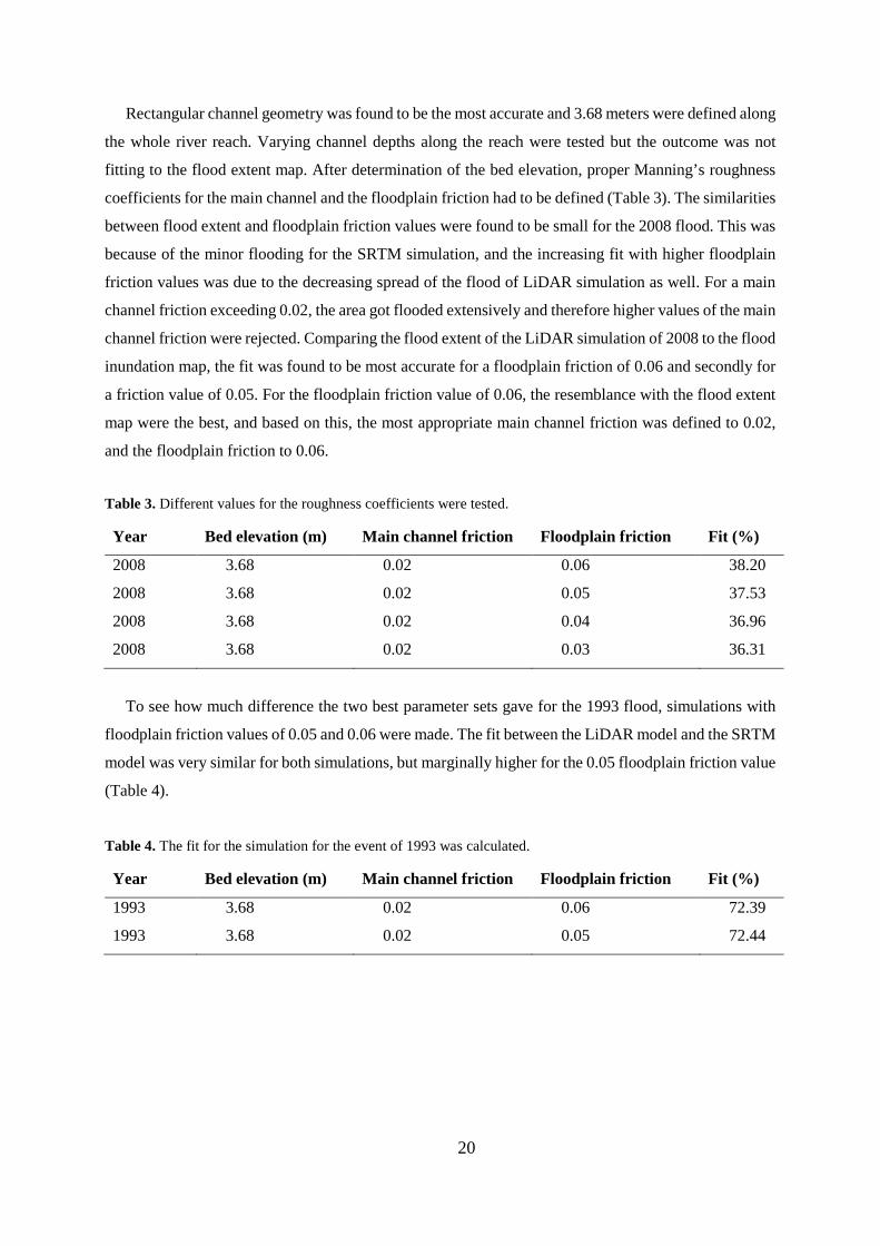
5.2 Results of Calibration As mentioned above, the 2008 flood extent (compared to the LiDAR model outcome) was used for

model calibration. Different parameter values of Manning’s roughness coefficients and bed elevations

were tested and some of the results can be seen in the three tables below. A first estimate of the

Manning’s coefficients were defined; 0.02 for the main channel and 0.05 for the floodplain. In Table 2

it can be seen that different bed elevations were simulated and the resulting fit. The fit was calculated

through reclassification of flooded and dry fields, according to Table 1 and presented in Equation 3 in

section 4.4. Bed elevations of 2 meters and 3 meters gave fits of below 30 %, while bed elevation of 4

meters gave a fit of 65 %. However, such deep channel depth resulted in no flood occurrence at all for

the SRTM simulation. It was shown that a bed elevation of 3.68 meter, which was the depth at the

Louisiana gauging station (The Florida Times-Union, 2015), gave a reasonable fit and above all it

resulted in a flood inundation matching the observed flood inundation map.

Table 2. Simulations using different bed elevations.

131

132

133

134

135

136

0 10 20 30 40

Ele

vatio

n (m

eter

s)

Distance along river channel, upstream to downstream (km)

River surface elevation

LiDAR

SRTM

Year Bed elevation (m) Main channel friction Floodplain friction Fit (%)

2008 2.00 0.02 0.05 27.15

2008 3.00 0.02 0.05 22.13

2008 3.68 0.02 0.05 37.53

2008 4.00 0.02 0.05 65.27

20

Rectangular channel geometry was found to be the most accurate and 3.68 meters were defined along

the whole river reach. Varying channel depths along the reach were tested but the outcome was not

fitting to the flood extent map. After determination of the bed elevation, proper Manning’s roughness

coefficients for the main channel and the floodplain friction had to be defined (Table 3). The similarities

between flood extent and floodplain friction values were found to be small for the 2008 flood. This was

because of the minor flooding for the SRTM simulation, and the increasing fit with higher floodplain

friction values was due to the decreasing spread of the flood of LiDAR simulation as well. For a main

channel friction exceeding 0.02, the area got flooded extensively and therefore higher values of the main

channel friction were rejected. Comparing the flood extent of the LiDAR simulation of 2008 to the flood

inundation map, the fit was found to be most accurate for a floodplain friction of 0.06 and secondly for

a friction value of 0.05. For the floodplain friction value of 0.06, the resemblance with the flood extent

map were the best, and based on this, the most appropriate main channel friction was defined to 0.02,

and the floodplain friction to 0.06.

Table 3. Different values for the roughness coefficients were tested.

Year Bed elevation (m) Main channel friction Floodplain friction Fit (%)

2008 3.68 0.02 0.06 38.20

2008 3.68 0.02 0.05 37.53

2008 3.68 0.02 0.04 36.96

2008 3.68 0.02 0.03 36.31

To see how much difference the two best parameter sets gave for the 1993 flood, simulations with

floodplain friction values of 0.05 and 0.06 were made. The fit between the LiDAR model and the SRTM

model was very similar for both simulations, but marginally higher for the 0.05 floodplain friction value

(Table 4).

Table 4. The fit for the simulation for the event of 1993 was calculated.

Year Bed elevation (m) Main channel friction Floodplain friction Fit (%)

1993 3.68 0.02 0.06 72.39

1993 3.68 0.02 0.05 72.44

21

5.3 Stage Evaluation Looking at stage differences and inundated flood extents in the simulations, it can be seen that the

simulated water stages did not correspond to the available observed water stages. According to

observations of different flood events, the water stages at the upstream station Lock & Dam 22 and the

middle station at Louisiana are at similar levels. Downstream, at the station Lock & Dam 24, the water

stages increase (U.S. Army Corps of Engineers, 2015b). In Figure 9, examples of water stages during

one day of flooding events (at the three gauging stations) from different years can be seen. Notable is

that the observed conditions mismatches the decreasing trends of the simulations, meaning that the

simulated floods did not manage to capture the dynamics of observed events.

Figure 9. Real observation stages measured by U.S. Army Corps of Engineers (2015) displayed as solid lines are compared with simulated water stages, seen as dashed lines. The observed and simulated the water stage trends in the figure are representative for the common trends. The pattern of the observed stages is not obtained in the simulations.

The simulated flood peaks were not only showing incorrect trends, they were also too early and of a

too low magnitude, about 2 meters lower in general. For the flood of 2008 there was no observed data

over water stages to be found, but for the 1993 flood there were some flood peak values available. The

observed highest flood peak at the Louisiana gauging station occurred in July 29. Then the stage reached

8.60 meters (U.S. Army Corps of Engineers, 2015b). For the simulations of the 1993 flood, the peak for

the LiDAR simulation occurred on July 11 (stage height 6.83 meters) and for the SRTM simulation it

was on July 10 (stage height 6.80 meters). The discharges at Keokuk in 1993, which was the set as

inflow into the domain in the models, also peaked on July 10. The simulated trends did not correspond

to the observed trends, but comparison of simulated LiDAR and SRTM stages (Figure 10 and Figure

11) shows a very similar pattern for both the smaller and the bigger flood, despite of differences in flood

extents, and despite of different river surface elevations and flood bank elevations.

3

4

5

6

7

8

9

10

L&D 22 Louisiana L&D 24

Met

ers

Water stage trends

2009

2002

1986

1979

1993

1993

2008

2008

22

Figure 10. Simulated water stages at Louisiana gauging station during the flood in 2008. Manning’s coefficients used; main channel 0.02, floodplain 0.06.

Figure 11. Simulated water stages at Louisiana gauging station for the flood of 1993. Manning’s coefficients used; main channel 0.02, floodplain 0.06.

2

3

4

Met

ers

Simulated water stages 2008

LiDARSRTM

012345678

Met

ers

Simulated water stages 1993

LiDARSRTM

23

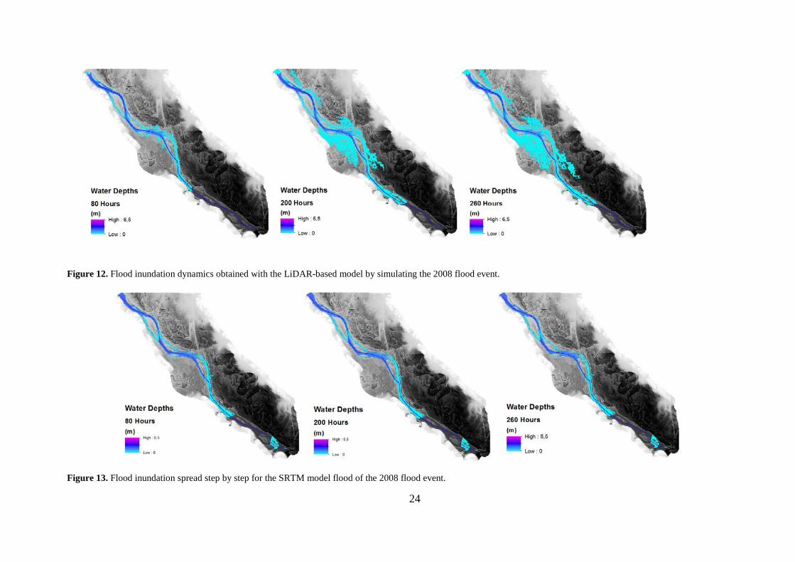
5.4 Flood Inundation Dynamics The outcomes of the models, after previous mentioned calibrations, are shown figures below, first for

the 2008 flood event and thereafter for the 1993 flood event. The flood inundation spread for the LiDAR

model is presented first and then for the SRTM model. Bed elevation was set to 3.68, the main channel

friction was 0.02 and the flooplain friction 0.06. For more detailed information of the flood inundation

dynamics see maps in appendix B.

For the smaller flood event of 2008, the flood inundation during 11 days, March 16 to March 27 was

simulated. March 16 was set to day zero and in total 264 hours was simulated. For the LiDAR simulation

the flooding starts to spread after 140 hours, i.e. March 22. After 260 hours the area close to the river

channel was inundated, similarly to the flood inundation map from the 2008 flood (Figure 12). However,

for the SRTM simulation the extent of the flooding was minimal and the floodplain is almost not flooded

at all (Figure 13).

For the 1993 flood event, the period from March 4 to August 1 was simulated. During it, severe

flooding occurred in both LiDAR-based and SRTM-based model simulations. As for the smaller flood

event of 2008, the flood extent for the LiDAR simulation was greater than for the SRTM simulation

(Figure 14 and Figure 15).

24

Figure 12. Flood inundation dynamics obtained with the LiDAR-based model by simulating the 2008 flood event.

Figure 13. Flood inundation spread step by step for the SRTM model flood of the 2008 flood event.

25

Figure 14. Flood inundation dynamics for the LiDAR model flood of the 1993 flood event.

Figure 15. Flood inundation dynamics for the SRTM model flood of the 1993 flood event.

26

5.5 Classification of Flooded Areas The LIDAR and SRTM simulations were put togeter for the calculation of the fit. As stated in Table 1

presented in section 4.4, class A represents areas flooded in both simulations, and is here displayed in

dark blue. Class B, colored green, is areas only flooded in the SRTM simulation and class C, light blue

colored, represents areas only flooded in the LiDAR simulation. Class D, grey colored, is areas that are

dry in both simulations.

5.5.1 Fit of the 2008 Flood Event In Figure 16 it can be seen that it is mostly the flood of the LiDAR model that spreads over the

floodplain.

Figure 16. Reclassified fields during different times of the 2008 flood event.

In Table 5 the fit is calculated, and the fit decreases over the time of the flood event, due to the

floodplain inundation of the LIDAR simulation but not of the SRTM simulation.

Table 5. Calculation of the fit between the models during different times of the flood event.

Year 2008 Class A B C D Fit (%) 20 Hours Value 2387 627 384 61896 70.25 80 Hours Value 3049 586 762 60897 69.34 140 Hours Value 3278 421 1841 59754 59.17 200 Hours Value 3285 395 4193 57421 41.73 260 Hours Value 3042 560 4362 57330 38.20

27

5.5.2 Fit of the 1993 Flood Event In Figure 17 it can be seen that there is extensive flooding for both floods, but that flood extent obtained

with the LiDAR model is greater.

Figure 17. Reclassified fields during different times of the 1993 flood event.

At the basis of the values received during the reclassification (Figure 17), the fit was calculated

(Table 6). Also for the 1993 flood event the fit is high in the beginning of the flood when the river

channel is filling up and flooding is starting to spread. However, in contrast with the fit for the 2008

flood event, the fit for the 1993 flood increases over the time of the flood event because of the delayed

spreading of the flood of the SRTM simulation.

Table 6. Calculation of the fit between the models during different times of the flood event.

Year 1993 Class A B C D Fit (%) 2 Days Value 3846 932 3133 57383 48.62 10 Days Value 2733 987 10714 50860 18.94 40 Days Value 10747 274 33745 20528 24.01 80 Days Value 17417 25519 505 21853 40.09 150 Days Value 38452 166 14500 12176 72.39

28

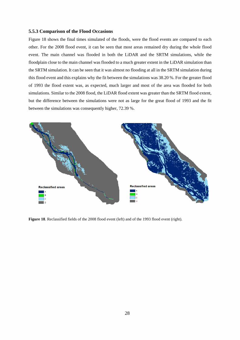
5.5.3 Comparison of the Flood Occasions Figure 18 shows the final times simulated of the floods, were the flood events are compared to each

other. For the 2008 flood event, it can be seen that most areas remained dry during the whole flood

event. The main channel was flooded in both the LiDAR and the SRTM simulations, while the

floodplain close to the main channel was flooded to a much greater extent in the LiDAR simulation than

the SRTM simulation. It can be seen that it was almost no flooding at all in the SRTM simulation during

this flood event and this explains why the fit between the simulations was 38.20 %. For the greater flood

of 1993 the flood extent was, as expected, much larger and most of the area was flooded for both

simulations. Similar to the 2008 flood, the LiDAR flood extent was greater than the SRTM flood extent,

but the difference between the simulations were not as large for the great flood of 1993 and the fit

between the simulations was consequently higher, 72.39 %.

Figure 18. Reclassified fields of the 2008 flood event (left) and of the 1993 flood event (right).

29

6. Discussion Previous studies have shown that there is a strong need of flood inundation mapping and monitoring in

data-poor areas of the world (Sanders 2007; Di Baldassarre et al. 2011; Padi et al., 2011; Yan et al.

2013). When it comes to testing the usability of a modelling code, in this case using the model with

another type of input resolution data than constructed for, several case studies has to be conducted.

DEMs derived from low resolute remote sensing data, such as the SRTM, are expected to offer

invaluable possibilities for further advancements of the flood inundation modelling, to take a step

towards a comprehensive, worldwide and cheaper tool for the prediction of flood risks. Nevertheless,

this is a topic surrounded of uncertainties, and there is a discussion whether the limitations and the

inaccuracy of the topographic information are too high, and that this makes it impossible to predict

hazardous events. To contribute to the ongoing research on this subject, a comparative case study was

conducted in a river reach of the Mississippi (USA). The model was calibrated according to the LiDAR

based simulation, and it was found that a river bed elevation of 3.68 meters and Manning’s coefficients

of 0.02 for the main channel and 0.06 for the floodplain friction were suitable.

The estimation the roughness coefficients was a source of uncertainty. Due to time-consuming

simulations, some up to two hours, a statistically analysis of the best match between Manning’s

coefficients for the main channel and for the floodplain, could not be done and manual calibration was

the only approach possible.

There were also other uncertainties, sensitivities and limitations too that had to be considered in this

study, most importantly the uncertainty and errors on the original input topography data, i.e. the LiDAR

and SRTM DEMs. It was a great interest to investigate the height differences between the two DEMs

uses, because of the impact on flood inundation spread. It was shown that most of the floodplain

topography was similar in both DEMs, where the difference was below 1 meter. There are very big

height differences in the mountainous areas at the borders of the reach (up to 70 meters), and also height

differences of up to 15 meters just next to the river channel. Those differences close to the main channel

can explain the differences in flood extent for the smaller flood of 2008, when the water could not flood

those areas and continue to the parts of the floodplain where the elevation was similar to the elevation

of the LiDAR DEM. This was further enhanced by the lower elevation of the river surface of the SRTM

DEM compared to the LiDAR DEM. The root mean square error (RMSE) was calculated to be 7.79

meters for the whole case study area. The small height differences of the floodplain area together with

the large differences in the mountainous area, together sums up in the RMSE. For flood inundation

extent, the spatial distribution of the height error is very important and therefore the RMSE can be very

misleading. A height error next to the river channel can influence a lot on the spread of the flood while

a height error in a mountain area does not make any difference at all.

30

Also the processing of the input data, in order to match the input file format and to make the

comparison possible, introduces additional uncertainties. The DEMs had for example to be aggregated

in ARC GIS and the pixels reclassified to flooded and dry during the validation.

The simulated flood water stages did not capture the trends of the observed flood water stages. For

the 1993 simulations, were data of record stages were available, the simulated peaks did not occurred

on the right dates. A possible explanation to this is the free downstream boundary condition defined by

the 2D model. It was defined as free due to insufficient data available, i.e. other boundary conditions,

such as hydrographs, were not possible. However, it has to be pointed out that the aim of this study was

not to make a model over the Mississippi River; it was to test the usability of SRTM DEMs. Therefore,

those limitations were of less importance for this study.

In previous research by Yan et al. (2013), a problem was that the predicted water stages differed

between the models. This was not a problem in this study, the simulated water stages for the two models

showed a very good correspondence and both the smaller and the larger floods had similar water stage

trends over the time span of the flood occurrences. Even though the channel water surface elevations of

the SRTM model were lower and the banks were higher, the model managed to capture the water stages

of the LiDAR model very well.

Concerning flood inundation extents, it was found that the simulations corresponded to each other to

a larger extent for the greater flood of 1993, where the fit between the LiDAR and SRTM simulations

were 72 %. For the smaller flood of 2008 the fit was significantly lower, 38 %. These results support

the conclusions of several previous studies; that remote sensing tools can be used with higher accuracy

for large scale catchment areas and larger flood events (Schumann et al., 2008). For small magnitude

floods the small variations in topography elevations between the DEMs have shown to contribute to

major differences for the flooding extent. The micro topography then plays an important role for the

behavior and the performance of the model is affected. This was also supported by the increasing fit

during the flood occasion of the bigger flood of 1993. It took longer time for the flood in the SRTM

simulation to start spreading, and the smaller flow in the beginning was probably prevented by the “bank

barriers” to spread, but after some time the SRTM-based model simulated a flood extent similar to the

one simulated by the LiDAR-based model. As mentioned in the background section 3.1, the vegetation

influences the accuracy of the SRTM DEMs and a percentage of the elevation height could be subtracted

from the SRTM DEM. That could have been shown to increase the fit additionally, but due to the flat

topography of the case study area, were most of the floodplain were made up by fields and arable land,

this is unsure. Nevertheless, the relatively good performance of the SRTM model in this case study can

be linked to the flat topography. The question that remains, however, is what the value of remote sensing

methods for flood inundation actually is. Generally, greater floods affect larger amount of people and

damage more property and infrastructure, with the consequence that the inaccuracy in simulating smaller

flood inundations is less critical.

31

The uncertainties of remote sensing data has to be further developed and analyzed, to enable use with

higher understanding and better knowledge of potential errors. Also, LiDAR simulations are not the

same as observed inundation extents; it is also a prediction containing uncertainties. Therefore the

importance of extensive testing and evaluation is high. It is also probable that the SRTM data vary in

quality for different areas of the world and also within study areas, and therefore case studies for areas

spread over different parts of the world would be recommended.

This study has shown results supporting the hypotheses of the usability of low resolution topography

data for flood inundation modelling. It is therefore a step further in the direction of improving flood risk

assessment all over the world. SRTM is freely, globally available online and that is a big advantage.

32

7. Conclusions In this study, the usability of remote sensing topography data (i.e. SRTM) to support flood inundation

modelling has been tested by comparing the results of a SRTM-based model with the ones obtained with

a reference model built on high quality topography data (LiDAR). The case study conducted indicates

that that flood inundation modelling with remote sensing data is more accurate for high magnitude flood

events than for smaller flood events. The fit of inundation extents, between the last stages of the flood

events, was for the big flood simulated in this study 72 %, while it was 38 % for the small flood

simulated. Details in the topography are more influential for smaller flood events than for larger ones.

Consequently, differences in topography data affect the flood inundation extent of smaller floods to a

higher degree. The major importance of micro topography for smaller flood events is one of the major

conclusions in this study. Because of the limited time and computational power an automatic calibration,

for example using Monte Carlo runs, was not possible and the calibration was made manually. However,

this is not considered a major limitation in view of the aim of this thesis. This study did not intent to

build a faultless model of a part of the Mississippi River, but rather benchmark a SRTM-model with a

model based on state-of-the-art topography (LiDAR). A suggestion for future studies can be to do the

calibration for the LiDAR model and for the SRTM model separately, to see what impact this has for

the behavior of the floods. Remote sensing for flood inundation modelling has a great potential,

especially to support the modelling of bigger flood events. Using satellite data for flood inundation

modelling can open up interesting possibilities. For instance, it might make it possible to build flood

maps to a lower cost and estimate risks in areas that lack the economic resources needed for flood

inundation modelling today. When no other data with higher accuracy and precision is available, this

study suggests that predictions made with globally remote sensing data are still better than the option of

making no predictions at all. Also, according to the development and increasing availability and

precision of the remote sensing data, there are high expectations of the future and of increasing accuracy

when using satellites for floodplain inundation modelling. To further validate the results and support

this conclusion, more case studies of rivers systems with different properties, different flood magnitudes,

vegetation covers and river scales, are needed.

33

8. Acknowledgements I want to thank Giuliano Di Baldassarre for supervising and inspiration, Kun Yan for useful advises and

Thomas Grabs for valuable comments. I also want to thank Janis Kreiselmeier for all the discussions we

have had along the thesis process and for the ARC GIS help he offered me. I am also grateful to Linnéa

Anglemark at Språkverkstaden for enthusiastic language guidance, and to my opponent Kristin Larson

for comments and support. Finally I want to thank USGS and CGIAR International Research Centers

for providing data freely available online.

34

9. References Alsdorf, D, Dunne, T, Melack, J, Smith, L & Hess, L 2005, 'Diffusion modeling of recessional flow on central Amazonian floodplains' Geophysical Research Letters, vol. 32, no. 21, L21405, doi: 10.1029/2005GL024412 Alsdorf, D, Rodríguez, E, Lettenmaier, D 2007, 'Measuring surface water from space', Reviews of Geophysics, vol. 45, no. 2, RG2002, doi:10.1029/2006RG000197 Bates, P, De Roo, A 2000, 'A simple raster-based model for flood inundation simulation', Journal of Hydrology, vol. 236, no. 1-2, pp. 54-77, doi:10.1016/S0022-1694(00)00278-X Bates, P, Trigg, M, Neal, J, Dabrowa, A 2013, 'LISFLOOD-FP User Manual (Code release 5.9.6)', School of Geographical Sciences, University of Bristol, University Road, Bristol, BS8 1SS, UK Baugh, C, Bates, P, Schumann, G, Trigg, M 2013, 'SRTM vegetation removal and hydrodynamic modeling accuracy', Water Resources Research, vol. 49, no. 9, pp. 5276–5289, doi:10.1002/wrcr.20412 Brakenridge, G, Knox, J, Paylor, E, Magilligan, F 1994, 'Radar remote sensing aids study of the Great Flood of 1993', Eos, Transactions American Geophysical Union, vol. 75, no. 45, pp. 521–527, doi:10.1029/EO075i045p00521 Castellarin, A, Domeneghetti, A, Brath, A 2011, 'Identifying robust large-scale flood risk mitigation strategies: A quasi-2D hydraulic model as a tool for the Po river', Physics and Chemistry of the Earth, Parts A/B/C, Recent Advances in Mapping and Modelling Flood Processes in Lowland Areas, vol. 36, no. 7-8, pp. 299–308, doi:10.1016/j.pce.2011.02.008 Centers for Disease Control and Prevention (CDC) 1989, 'International Notes Health Assessment of the Population Affected by Flood Conditions -- Khartoum, Sudan', Morbidity and Mortality Weekly Report (MMWR), Vol. 1988, No. 51&52, pp. 785-788, viewed 20 March 2015, http://www.cdc.gov/mmwr/preview/mmwrhtml/00001323.htm Consortium for Spatial Information (CGIAR-CSI) 2004, SRTM 90m Digital Elevation Data, viewed 20 March 2015, http://srtm.csi.cgiar.org/SELECTION/inputCoord.asp Dartmouth Flood Observatory 2009, 'DFO Event # 2008-035 - US Midwest - Rapid Response Inundation Map', Dartmouth College, viewed 20 March 2015, http://www.dartmouth.edu/~floods/images/2008035USmidwest.jpg Dartmouth Flood Observatory 2010, 'Current and Past Flooding, W100N40', Dartmouth College, viewed 20 March 2015, http://www.dartmouth.edu/~floods/hydrography/W100N40.html Di Baldassarre, G, Montanari, A, Lins, H, Koutsoyiannis, D, Brandimarte, L, Blöschl, G 2010, 'Flood fatalities in Africa: From diagnosis to mitigation', Geophysical Research Letters, vol. 37, no. 22, L22402, doi:10.1029/2010GL045467 Di Baldassarre, G, Schumann, G, Brandimarte, L, Bates, P 2011, 'Timely Low Resolution SAR Imagery To Support Floodplain Modelling: a Case Study Review', Surveys in Geophysics, vol. 32, no. 3, pp. 255–269, doi:10.1007/s10712-011-9111-9 Dottori, F, Todini, E 2011, 'Developments of a flood inundation model based on the cellular automata approach: Testing different methods to improve model performance', Physics and Chemistry of the Earth, Parts A/B/C, Recent Advances in Mapping and Modelling Flood Processes in Lowland Areas, vol. 36, no. 7-8, pp. 260–280, doi:10.1016/j.pce.2011.02.004

35

Farr, T, Kobrick, M, 2000, 'The Shuttle Radar Topography Mission: A Global DEM', Jet Propulsion Laboratory, California Institute of Technology, viewed 24 March 2015, http://ntrs.nasa.gov/archive/nasa/casi.ntrs.nasa.gov/20000053500.pdf Federal Emergency Management Agency (FEMA) 2015, 'Risk Mapping, Assessment and Planning (Risk MAP)', U.S. Department of Homeland Security, viewed 20 March 2015, https://www.fema.gov/risk-mapping-assessment-and-planning-risk-map Google Earth, 2014, 'Image Landsat', Google Earth, viewed 15 March 2015 Jung, H, Alsdorf, D, Moritz, M, Lee, H, Vassolo, S 2011, 'Analysis of the relationship between flooding area and water height in the Logone floodplain', Physics and Chemistry of the Earth, Parts A/B/C, Recent Advances in Mapping and Modelling Flood Processes in Lowland Areas, vol. 36, no. 7-8, pp. 232–240, doi:10.1016/j.pce.2011.01.010 Lott, N 1993, 'The summer of 1993: flooding in the midwest and drought in the southeast', National Climatic Data Center, Technical Report, No. 93-04, viewed 6 March 2015, http://www1.ncdc.noaa.gov/pub/data/techrpts/tr9304/tr9304.txt Mason, D, Schumann, G, Bates, P 2011, Data utilisation in flood inundation modelling, in: Flood Risk Science and Management, e-book, pp. 211–233, Wiley-Blackwell, Chichester, UK. Ohl, C, Tapsell, S 2000, 'Flooding and human health', British Medical Journal, Vol. 321, No. 7270, pp. 1167–1168, viewed 20 March 2015, http://www.ncbi.nlm.nih.gov/pmc/articles/PMC1118941/ Padi, P, Di Baldassarre, G, Castellarin, A 2011, 'Floodplain management in Africa: Large scale analysis of flood data' Physics and Chemistry of the Earth, Parts A/B/C, Recent Advances in Mapping and Modelling Flood Processes in Lowland Areas, vol. 36, no. 7-8, pp. 292–298, doi:10.1016/j.pce.2011.02.002 Patro, S, Chatterjee, C, Singh, R, Raghuwanshi, N 2009, 'Hydrodynamic modelling of a large flood-prone river system in India with limited data', Hydrological Processes, vol. 23, no. 19, pp. 2774–2791, doi:10.1002/hyp.7375 Plate, E 2002, 'Flood risk and flood management', Journal of Hydrology, Advances in Flood Research, vol. 267, no. 1-2, pp. 2-11, doi:10.1016/S0022-1694(02)00135-X Rodríguez, E, Morris, C, Belz, E 2006, 'A Global Assessment of the SRTM Performance. Photogramm', Photogrammetric Engineering & Remote Sensing, American Society for Photogrammetry and Remote Sensing, vol. 2006, no. 3, pp. 249–260, viewed 6 May 2015, http://www.asprs.org/a/publications/pers/2006journal/march/2006_mar_249-260.pdf Sanders, B 2007, Evaluation of on-line DEMs for flood inundation modeling', Advances in Water Resources, vol. 30, no. 8, pp. 1831–1843, doi:10.1016/j.advwatres.2007.02.005 Schumann, G, Matgen, P, Cutler, M, Black, A, Hoffmann, L, Pfister, L 2008, 'Comparison of remotely sensed water stages from LiDAR, topographic contours and SRTM', ISPRS Journal of Photogrammetry and Remote Sensing, vol. 63, no. 3, pp. 283–296, doi:10.1016/j.isprsjprs.2007.09.004 Smith, L 1997, 'Satellite remote sensing of river inundation area, stage, and discharge: a review', Hydrological Processes, vol 11, no. 10, pp. 1427–1439. doi:10.1002/(SICI)1099-1085(199708)11:10<1427::AID-HYP473>3.0.CO;2-S

36

Smith, M, Edwards, E, Priestnall, G, Bates, P 2006, 'Exploitation of new data types to create digital surface models for flood inundation modelling', FRMRC Research Report UR3 Project, No. UR3, pp. 1-78, Flood Risk Management Research Consortium, University of Manchester, Manchester, http://web.sbe.hw.ac.uk/frmrc/downloads/UR3%20signed%20off.pdf Stephens, E, Bates, P, Freer, J, Mason, D 2012, 'The impact of uncertainty in satellite data on the assessment of flood inundation models', Journal of Hydrology, vol. 414–415, pp. 162–173, doi:10.1016/j.jhydrol.2011.10.040 Straatsma, M, Huthoff, F 2011, 'Uncertainty in 2d hydrodynamic models rom errors in roughness paramerterization based on aerial images', Physics and Chemistry of the Earth, Parts A/B/C, Recent Advances in Mapping and Modelling Flood Processes in Lowland Areas, vol. 36, no. 7-8, pp. 324–334, doi: 10.1016/j.pce.2011.02.009 Sun, G, Ranson, K, Kharuk, V, Kovacs, K 2003, 'Validation of surface height from shuttle radar topography mission using shuttle laser altimeter', Remote Sensing of Environment, vol. 88, no. 4, pp. 401-411, doi:10.1016/j.rse.2003.09.001 The Florida Times-Union 2015, Mississippi River near Louisiana, MO (Gauge LUSM7), viewed 24 March 2015, http://weather.jacksonville.com/rivers/gauge/LUSM7.html United Nations International Strategy for Disaster Reduction (UNISDR) 2009, 'UNISDR Terminology on Disaster Risk Reduction', United Nations, pp. 1-31, viewed 10 March 2015, http://www.unisdr.org/files/7817_UNISDRTerminologyEnglish.pdf Upper Midwest Environmental Science Center (UMESC) 2014, About the Upper Mississippi River System, viewed 5 May 2015, http://www.umesc.usgs.gov/umesc_about/about_umrs.html U.S. Army Corps of Engineers 2015a, The Mississippi Drainage Basin, viewed 5 May 2015, http://www.mvn.usace.army.mil/Missions/MississippiRiverFloodControl/MississippiRiverTributaries/MississippiDrainageBasin.aspx U.S. Army Corps of Engineers 2015b, Mississippi River & Passes, RiverGages.com, viewed 20 March 2015, http://www2.mvr.usace.army.mil/WaterControl/new/layout.cfm U.S Geological Survey (USGS) 2013, HydroSHEDS, viewed 5 May 2015, http://hydrosheds.cr.usgs.gov/dataavail.php U.S Geological Survey (USGS) 2014, Reach 2 - Navigation Pool 24 - Upper Mississippi River, viewed 20 March 2015, http://www.umesc.usgs.gov/rivers/upper_mississippi/reach_2/pool_24/pool_24.html U.S Geological Survey (USGS) 2015, USGS 05474500 Mississippi River at Keokuk, IA, viewed 8 June 2015, http://waterdata.usgs.gov/ia/nwis/dv/?site_no=05474500 Wechsler, S 2007, 'Uncertainties associated with digital elevation models for hydrologic applications: a review', Hydrology and Earth System Sciences, vol. 11, no. 4, pp. 1481–1500, doi:10.5194/hess-11-1481-2007 Willmott, C, Matsuura, K 2005, 'Advantages of the mean absolute error (MAE) over the root mean square error (RMSE) in assessing average model performance', Inter-Research, vol. 2005, no. 30, pp. 79–82, doi:10.3354/cr030079 Winsemius, H, Van Beek, L, Jongman, B, Ward, P, Bouwman, A 2013, 'A framework for global river flood risk assessments', Hydrology and Earth System Sciences, vol. 17, no. 5, pp. 1871–1892, doi:10.5194/hess-17-1871-2013

37

Yamazaki, D, Kanae, S, Kim, H, Oki, T 2011, 'A physically based description of floodplain inundation dynamics in a global river routing model', Water Resources Research, vol. 47, no. 4, W04501, doi:10.1029/2010WR009726 Yamazaki, D, Baugh, C, Bates, P, Kanae, S, Alsdorf, D, Oki, T 2012, 'Adjustment of a spaceborne DEM for use in floodplain hydrodynamic modeling', Journal of Hydrology, vol. 436-437, pp. 81–91, doi:10.1016/j.jhydrol.2012.02.045 Yan, K, Di Baldassarre, G, Solomatine, D 2013, 'Exploring the potential of SRTM topographic data for flood inundation modelling under uncertainty', Journal of Hydroinformatics, vol. 15, no. 3, pp. 849, doi:10.2166/hydro.2013.137

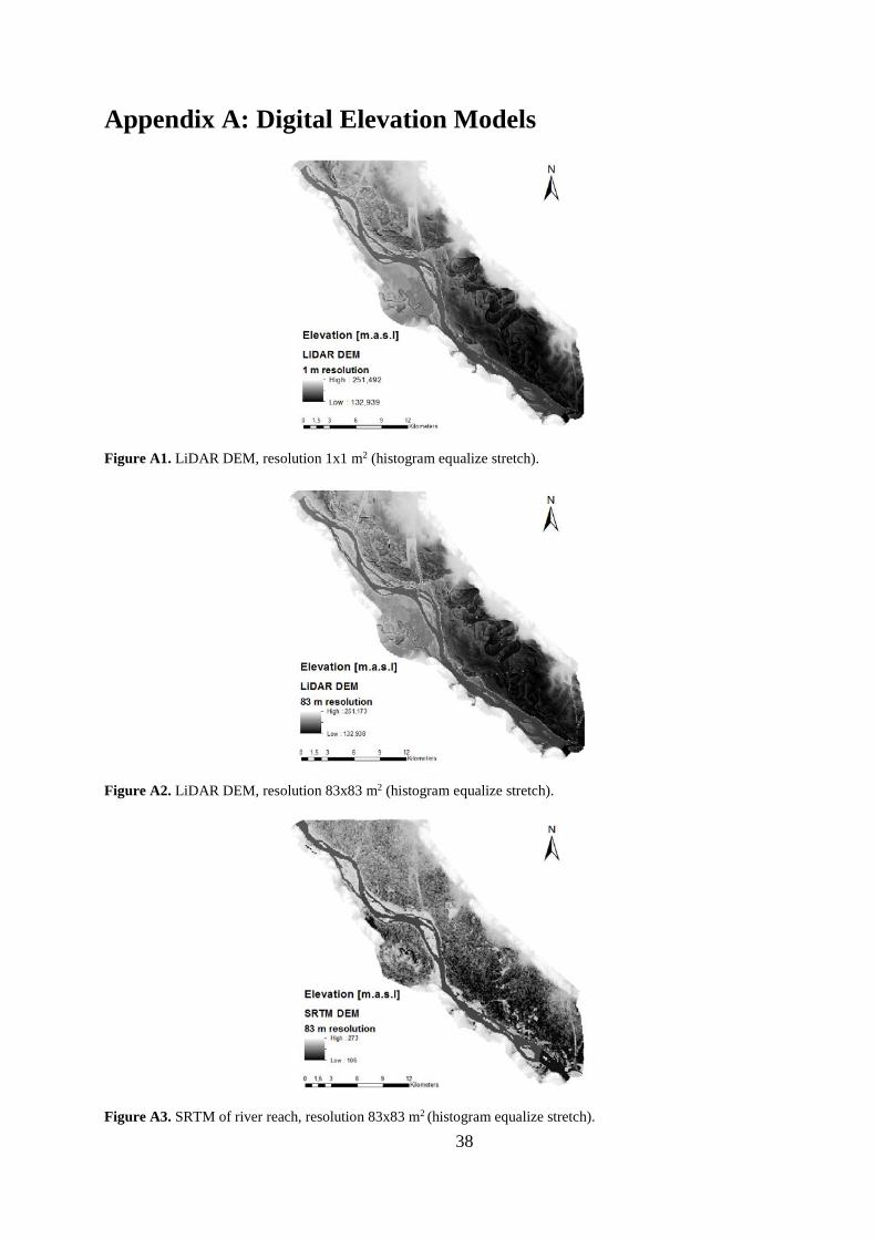
38

Appendix A: Digital Elevation Models

Figure A1. LiDAR DEM, resolution 1x1 m2 (histogram equalize stretch).

Figure A2. LiDAR DEM, resolution 83x83 m2 (histogram equalize stretch).

Figure A3. SRTM of river reach, resolution 83x83 m2 (histogram equalize stretch).

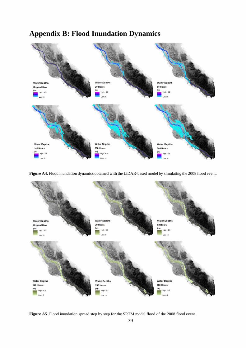
39

Appendix B: Flood Inundation Dynamics

Figure A4. Flood inundation dynamics obtained with the LiDAR-based model by simulating the 2008 flood event.

Figure A5. Flood inundation spread step by step for the SRTM model flood of the 2008 flood event.

40

Figure A6. Comparison of flood inundation dynamics by using the two models to simulate the 2008 flood event.

Figure A7. Flood inundation dynamics for the LiDAR model flood of the 1993 flood event.

41

Figure A8. Flood inundation dynamics for the SRTM model flood of the 1993 flood event.

Figure A9. Comparison of the flood inundation dynamics for the two models of the 1993 flood event.

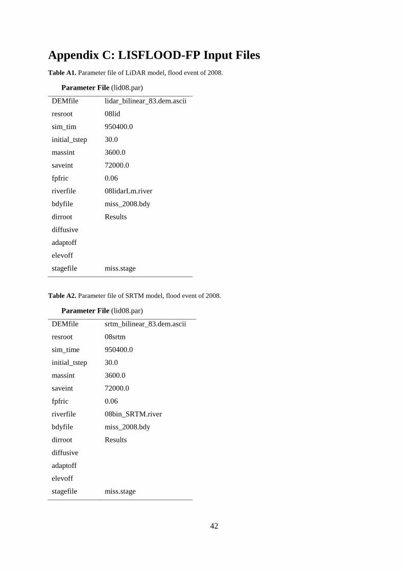
42

Appendix C: LISFLOOD-FP Input Files Table A1. Parameter file of LiDAR model, flood event of 2008.

Parameter File (lid08.par)

DEMfile lidar_bilinear_83.dem.ascii

resroot 08lid

sim_tim 950400.0

initial_tstep 30.0

massint 3600.0

saveint 72000.0

fpfric 0.06

riverfile 08lidarLm.river

bdyfile miss_2008.bdy

dirroot Results

diffusive

adaptoff

elevoff

stagefile miss.stage

Table A2. Parameter file of SRTM model, flood event of 2008.

Parameter File (lid08.par)

DEMfile srtm_bilinear_83.dem.ascii

resroot 08srtm

sim_time 950400.0

initial_tstep 30.0

massint 3600.0

saveint 72000.0

fpfric 0.06

riverfile 08bin_SRTM.river

bdyfile miss_2008.bdy

dirroot Results

diffusive

adaptoff

elevoff

stagefile miss.stage

43

Table A3. Parameter file of LiDAR model, flood event of 1993.

Parameter File (151lidar.par)

DEMfile lidar_bilinear_83.dem.ascii

resroot lid93

sim_time 12960000.0

initial_tstep 30.0

massint 86400.0

saveint 172800.0

fpfric 0.06

riverfile lidarLm.river

bdyfile 4mars_1aug_1993.bdy

dirroot Results_4mars_1aug

diffusive

adaptoff

elevoff

stagefile miss.stage

Table A4. Parameter file of SRTM model, flood event of 1993.

Parameter File (151srtm.par)

DEMfile srtm_bilinear_83.dem.ascii

resroot srtm93

sim_time 12960000.0

initial_tstep 30.0

massint 86400.0

saveint 172800.0

fpfric 0.06

riverfile SRTMLm.river

bdyfile 4mars_1aug_1993.bdy

dirroot Results_4mars_1aug

diffusive

adaptoff

elevoff

stagefile miss.stage

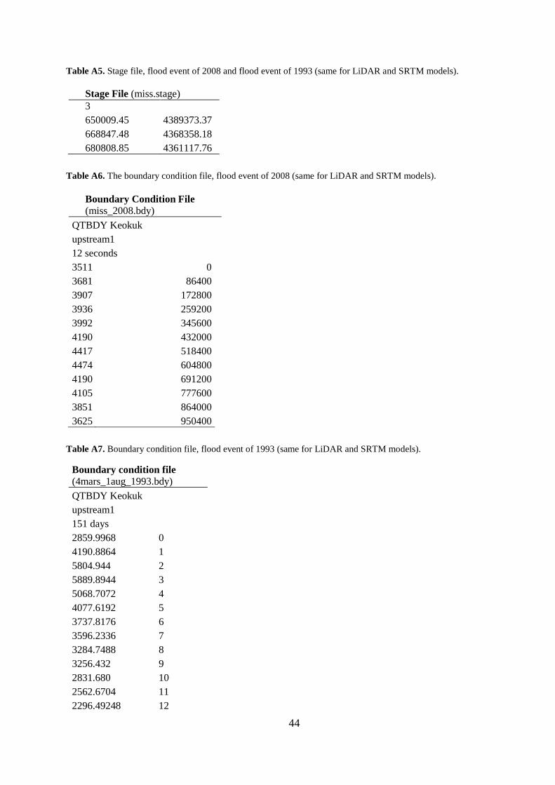
44

Table A5. Stage file, flood event of 2008 and flood event of 1993 (same for LiDAR and SRTM models).

Stage File (miss.stage) 3 650009.45 4389373.37 668847.48 4368358.18 680808.85 4361117.76

Table A6. The boundary condition file, flood event of 2008 (same for LiDAR and SRTM models). Boundary Condition File (miss_2008.bdy)

QTBDY Keokuk upstream1 12 seconds 3511 0 3681 86400 3907 172800 3936 259200 3992 345600 4190 432000 4417 518400 4474 604800 4190 691200 4105 777600 3851 864000 3625 950400

Table A7. Boundary condition file, flood event of 1993 (same for LiDAR and SRTM models).

Boundary condition file (4mars_1aug_1993.bdy) QTBDY Keokuk upstream1 151 days 2859.9968 0 4190.8864 1 5804.944 2 5889.8944 3 5068.7072 4 4077.6192 5 3737.8176 6 3596.2336 7 3284.7488 8 3256.432 9 2831.680 10 2562.6704 11 2296.49248 12

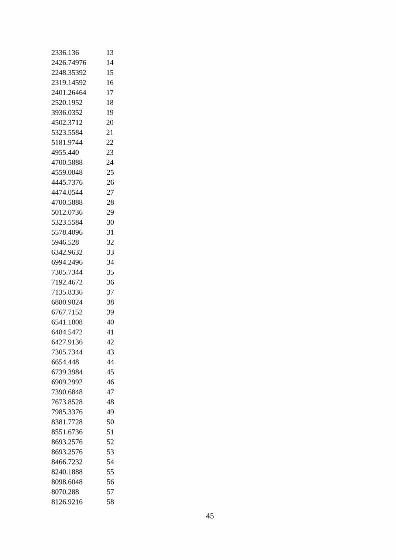
45

2336.136 13 2426.74976 14 2248.35392 15 2319.14592 16 2401.26464 17 2520.1952 18 3936.0352 19 4502.3712 20 5323.5584 21 5181.9744 22 4955.440 23 4700.5888 24 4559.0048 25 4445.7376 26 4474.0544 27 4700.5888 28 5012.0736 29 5323.5584 30 5578.4096 31 5946.528 32 6342.9632 33 6994.2496 34 7305.7344 35 7192.4672 36 7135.8336 37 6880.9824 38 6767.7152 39 6541.1808 40 6484.5472 41 6427.9136 42 7305.7344 43 6654.448 44 6739.3984 45 6909.2992 46 7390.6848 47 7673.8528 48 7985.3376 49 8381.7728 50 8551.6736 51 8693.2576 52 8693.2576 53 8466.7232 54 8240.1888 55 8098.6048 56 8070.288 57 8126.9216 58

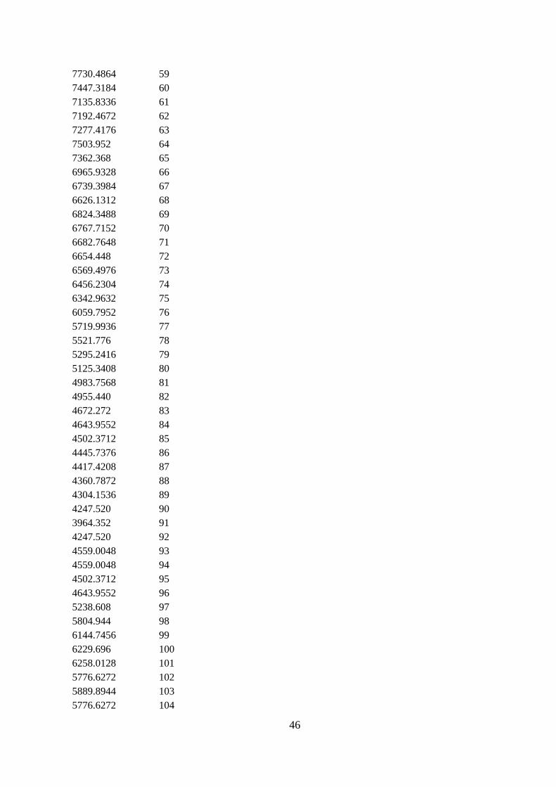
46

7730.4864 59 7447.3184 60 7135.8336 61 7192.4672 62 7277.4176 63 7503.952 64 7362.368 65 6965.9328 66 6739.3984 67 6626.1312 68 6824.3488 69 6767.7152 70 6682.7648 71 6654.448 72 6569.4976 73 6456.2304 74 6342.9632 75 6059.7952 76 5719.9936 77 5521.776 78 5295.2416 79 5125.3408 80 4983.7568 81 4955.440 82 4672.272 83 4643.9552 84 4502.3712 85 4445.7376 86 4417.4208 87 4360.7872 88 4304.1536 89 4247.520 90 3964.352 91 4247.520 92 4559.0048 93 4559.0048 94 4502.3712 95 4643.9552 96 5238.608 97 5804.944 98 6144.7456 99 6229.696 100 6258.0128 101 5776.6272 102 5889.8944 103 5776.6272 104

47

5691.6768 105 5663.3600 106 5691.6768 107 5776.6272 108 6031.4784 109 6201.3792 110 6427.9136 111 6569.4976 112 7645.5360 113 7872.0704 114 7815.4368 115 8098.6048 116 8155.2384 117 8551.6736 118 9316.2272 119 9457.8112 120 9656.0288 121 9854.2464 122 10052.464 123 10533.8496 124 11156.8192 125 11128.5024 126 11836.4224 127 12289.4912 128 11949.6896 129 11864.7392 130 11864.7392 131 11723.1552 132 11468.304 133 11439.9872 134 11383.3536 135 11213.4528 136 11015.2352 137 10873.6512 138 10873.6512 139 10986.9184 140 11043.552 141 11185.136 142 11326.720 143 11439.9872 144 11241.770 145 10873.6512 146 10278.9984 147 10278.9984 148 9089.6928 149 7957.0208 150

48

Table A8. River file for the LiDAR model, used in both flood simulations.

River File (08LidarLm.river) Tribs 42 650009.45 4389373.37 977.00 0.02 135.75 QVAR Upstream 1 650449.74 4388835.23 939.00 0.02 133.907 650865.58 4388297.09 563.00 0.02 133.886 651477.10 4387685.57 690.00 0.02 133.876 652162.00 4386951.74 666.00 0.02 133.741 653287.20 4386486.99 700.00 0.02 133.693 654143.33 4386120.08 938.00 0.02 133.617 654950.54 4385802.08 495.00 0.02 133.662 655904.51 4385435.17 450.00 0.02 133.652 656467.11 4384701.34 461.00 0.02 133.661 656931.87 4383356.10 391.00 0.02 133.636 657152.02 4382255.26 655.00 0.02 133.576 657200.94 4381130.06 727.00 0.02 133.550 657959.23 4380053.78 4490.0 0.02 133.511 658888.74 4378977.50 770.00 0.02 133.465 659573.64 4378904.12 907.00 0.02 133.527 660747.77 4378757.35 1336.0 0.02 133.455 661921.89 4378537.21 1002.0 0.02 133.449 663389.54 4378047.99 1033.0 0.02 133.373 664025.52 4377216.32 454.00 0.02 133.456 664465.82 4376213.42 317.00 0.02 133.342 665077.34 4375063.76 410.00 0.02 133.342 665835.63 4373963.03 647.00 0.02 133.289 666471.61 4373327.04 854.00 0.02 133.281 666606.14 4372403.65 666.00 0.02 133.336 666728.45 4371033.84 717.00 0.02 133.231 667217.66 4370185.86 823.00 0.02 133.151 668089.20 4369214.31 528.00 0.02 133.029 668847.48 4368358.18 887.00 0.02 133.081 669972.68 4367379.75 1124.0 0.02 133.029 670877.73 4366817.15 1203.0 0.02 133.048 671954.01 4366083.32 1479.0 0.02 133.006 672810.14 4365618.56 803.00 0.02 132.921 673910.88 4365398.42 778.00 0.02 132.912 674669.17 4364884.74 1608.0 0.02 132.837 675672.06 4364248.76 1950.0 0.02 132.773 676846.19 4363906.30 859.00 0.02 132.697 677384.32 4363270.32 1189.0 0.02 132.631 677726.78 4362438.65 2372.0 0.02 132.714 678533.98 4361753.75 1960.0 0.02 132.691 679634.72 4361288.99 1361.0 0.02 132.759 680808.85 4361117.76 1221.0 0.02 132.364 FREE 0.000073

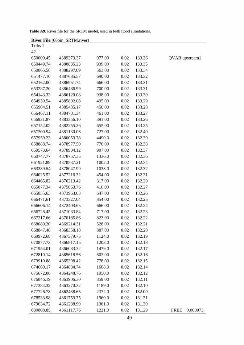
49

Table A9. River file for the SRTM model, used in both flood simulations.

River File (08bin_SRTM.river) Tribs 1 42 650009.45 4389373.37 977.00 0.02 133.36 QVAR upstream1 650449.74 4388835.23 939.00 0.02 133.35 650865.58 4388297.09 563.00 0.02 133.34 651477.10 4387685.57 690.00 0.02 133.32 652162.00 4386951.74 666.00 0.02 133.31 653287.20 4386486.99 700.00 0.02 133.31 654143.33 4386120.08 938.00 0.02 133.30 654950.54 4385802.08 495.00 0.02 133.29 655904.51 4385435.17 450.00 0.02 133.28 656467.11 4384701.34 461.00 0.02 133.27 656931.87 4383356.10 391.00 0.02 133.26 657152.02 4382255.26 655.00 0.02 133.25 657200.94 4381130.06 727.00 0.02 132.40 657959.23 4380053.78 4490.0 0.02 132.39 658888.74 4378977.50 770.00 0.02 132.38 659573.64 4378904.12 907.00 0.02 132.37 660747.77 4378757.35 1336.0 0.02 132.36 661921.89 4378537.21 1002.0 0.02 132.34 663389.54 4378047.99 1033.0 0.02 132.32 664025.52 4377216.32 454.00 0.02 132.31 664465.82 4376213.42 317.00 0.02 132.29 665077.34 4375063.76 410.00 0.02 132.27 665835.63 4373963.03 647.00 0.02 132.26 666471.61 4373327.04 854.00 0.02 132.25 666606.14 4372403.65 666.00 0.02 132.24 666728.45 4371033.84 717.00 0.02 132.23 667217.66 4370185.86 823.00 0.02 132.22 668089.20 4369214.31 528.00 0.02 132.21 668847.48 4368358.18 887.00 0.02 132.20 669972.68 4367379.75 1124.0 0.02 132.19 670877.73 4366817.15 1203.0 0.02 132.18 671954.01 4366083.32 1479.0 0.02 132.17 672810.14 4365618.56 803.00 0.02 132.16 673910.88 4365398.42 778.00 0.02 132.15 674669.17 4364884.74 1608.0 0.02 132.14 675672.06 4364248.76 1950.0 0.02 132.12 676846.19 4363906.30 859.00 0.02 132.11 677384.32 4363270.32 1189.0 0.02 132.10 677726.78 4362438.65 2372.0 0.02 132.00 678533.98 4361753.75 1960.0 0.02 131.31 679634.72 4361288.99 1361.0 0.02 131.30 680808.85 4361117.76 1221.0 0.02 131.29 FREE 0.000073

Examensarbete vid Institutionen för geovetenskaper ISSN 1650-6553