Condensed Matter Physics, 1998, Vol. 1, No 2(14), p. 257–309

The unified model description oforder-disorder and displacive structuralphase transitions

S.Stamenkovic

Institute of Nuclear Sciences, Laboratory for Theoretical Physics andCondensed Matter Physics, Belgrade, P.O.Box 522, Yugoslavia

Received July 7, 1998

A series of co-authors’ studies [1-7] devoted to the unified model descrip-tion of structural phase transitions (SPT) in ferroelectrics and related ma-terials are reviewed and partly innovated.

Starting from a general Hamiltonian of pair-coupled anharmonic (quar-tic) oscillators, together with the concept of local normal coordinates, aunified model description of both order-disorder and displacive types ofSPT-systems is proposed. Within the framework of the standard variationalprocedure, a hybridized pseudospin-phonon Hamiltonian is formulated byintroducing variables corresponding to phonon, magnon-like(flipping) andnonlinear(domain–wall-like) displacements of atoms participating in SPT.This is achieved by representing the cooperative atomic motion onto sev-eral quasiequilibrium positions (in the simplest case, two) as slow tunnellingdisplacement (decomposed into magnon-like and soliton-like deviations), inaddition to comparatively fast phonon oscillations around inhomogeneousmomentary rest positions, in turn induced by domain–wall-like (soliton) ex-citations.

The qualitative and quantitative analyses show that SPT (of the first orsecond order) can be either of a displacive (governed by a phonon softmode), order-disorder (governed by a tunnelling–magnon-like soft mode)or of a mixed type, depending on both the coupling energy between atomsand their zero-point vibrational energy. In the critical temperature region,the domain–wall-like excitations bring on the formation of microdomains(precursor clusters of the ordered phase) which induce SPT of the Isingtype universality class. The incomplete softening of the phonon or pseu-domagnon mode occurs and a central peak due to slow cluster relaxationappears in the spectral density of excitations.

Key words: structural phase transitions, order-disorder,displacivetransition

PACS: 63.70.+h, 77.80.Bh, 64.60.-i, 64.60.Cn

c© S.Stamenkovic 257

S.Stamenkovic

1. Introduction

Among numerous attempts to develop a unified microscopic theory of bothdisplacive and order-disorder structural phase transitions (SPTs), on the occasionof the 60th anniversary of Prof. Stasyuk’s birthday, our modest contribution [1-7]to the same problem in ferroelectric phase transitions is reviewed and partly inno-vated. To expose as clear as possible the basic proposals for a unified description ofSPT-systems and to better comprehend this peculiar problem in connection withits prospective development, we shall try to keep mostly to the original studiesof the co-authors’ group, with reference to other similar approaches cited in theco-authors’ publications. Accordingly, to acquire a rather contemporary unifieddescription of SPT (i.e. by novelizing the previous, original ones) it is convenientto employ the representation of local normal coordinates (LNCs) involving co-operative displacements of all the atoms in a primitive cell participating in thegiven critical (soft) vibrational mode. The LNCs are chosen so that they takeinto account the symmetry properties of the system, in order to be transformedby an irreducible representation of the point group of the primitive cell. Since thecorresponding order parameter of the system is transformed by the irreducible rep-resentation of the space group, such “conjunctive” coordinates can be consideredas the appropriate basis for describing SPT in the case when a single channel tran-sition (corresponding to a single-relevant irreducible representation) takes place inthe system we deal with throughout this review. With this substantial concept inmind, the grounds for the unified description of SPT become physically transpar-ent when one appreciates the natural generalization of the traditional concept ofatomic (including cooperative-like, represented by LNC) equilibrium states. In thenext step the time dependent LNC attributed to the cooperative atomic motionwithin the effective anharmonic multi-well potential is decomposed into a “slow”tunnelling displacement (being a momentary rest position, it consists of flipping–magnon-like and domain-wall–soliton-like deviations) and a comparatively “fast”superimposed deviation of the phonon type around the inhomogeneous clusterinduced by quasi-equilibrium positions (in the simplest case, two) inside the ef-fective one-particle potential. Thus, the ordering process is characterized by twoorder parameters - one reflecting the degree of the local precursor order (the av-erage population of equilibrium positions σz) and the other controlling the degreeof the long-range order (the average atomic displacement η).

The underlying approach is developed by incorporating the already adoptedLNC and the corresponding canonical momentum into the familiar model Hamil-tonian expressed in the form of effective pair-coupled anharmonic (in the simplestcase, quartic) oscillators. The further procedure is completed by a variational adap-tation of the microscopic model Hamiltonian (in the reduced phase space of coor-dinates and momenta) in various hybridized forms of phonon - tunnelling (pseu-dospin) - domain-wall (soliton) types separated in corresponding variables. On thebasis of a self-consistent phonon and a molecular-field approximations (namely, acombination of an independent-mode and independent-site evaluation schemes), a

258

Unified description of structural transitions

complete set of coupled self-consistent equations is obtained which enables one toestimate or to calculate (mainly numerically) all the physical (collective or local)quantities of the SPT-system (in the first place, both order parameters included).The qualitative and quantitative analyses of such a system of equations show thatthe SPT (of the first or second order) can be of a displacive (governed by a phononsoft mode), order-disorder (governed by a tunnelling - magnon-like soft mode) ora mixed type – depending predominantly on the reduced lattice coupling strengthand, in a lesser degree, on the ratio of the zero-point vibrational energy to theheight of the single-particle potential barrier. The possibility for phase transitionsof the both types occuring at zero temperature (quantum limits) is also outlined.In the case of a strongly anharmonic system the quantum limit of the displacivetype is examined in both, the ordered (σz = 1) and disordered (σz = 0) lattices.

Finally, it is analytically demonstrated that with the onset of criticality in all,order-disorder, displacive, as well as in mixed types of structural phase transitions,the domain-wall (soliton) excitations bring on the formation of microdomains (pre-cursor clusters of the ordered phase) which induce a phase transition of the Isinguniversality class. The incomplete softening of the phonon or/and pseudomagnonmode occurs and a central peak due to the slow cluster relaxation appears in theenergy spectrum of excitations.

2. Preliminaries

2.1. The elements of lattice dynamics at a structural transi tion

In agreement with the soft mode concept put forward independently by severalscholars in this field of solid state physics∗, a lattice undergoing transition is notstable in the harmonic approximation (it has a purely imaginary frequency for theoptical, i.e. polar mode) owing to the compensation of long-range attractive andshort-range repulsive forces. In that case in the symmetric phase the anharmonicinteraction, even if it is small, is necessary for the lattice vibrations to be stable.Therefore, in a consistent dynamical theory of SPT one must take into accountthe anharmonic interaction from the very beginning (already in the zero approx-imation), which requires the application of the methods of statistical mechanics,and depart from the simple mechanical approach adopted in the Born-Karmantheory. Meantime, a self-consistent phonon theory was developed ( mainly in con-nection with the study of quantum helium crystals) which was also applied to thedescription of structural transitions.

As it is well known, unlike the customary self-consistent (molecular) field ap-proximation, in the self-consistent phonon theory account is taken of fluctuationsof the order parameter, which play an important role in the second-order phasetransitions. It should be pointed out that the self-consistent phonon theory makesthe renormalised (due to fluctuations) Landau expansion for the free energy pos-sible and allows a self-consistent determination of the range of applicability of this

∗For a historical outline, for example, see [4] in [7].

259

S.Stamenkovic

method. The self-consistent phonon theory itself is generally considered for an ar-bitrary lattice (e.g., in [7,8]), where various theoretical applications to the concreteSPT model (we will also deal with them hereafter) are surveyed in detail. Such atheory is also adjusted to describe order-disorder SPT or transitions of the mixedtype which differ from the displacive ones only by a significantly higher degreeof unharmonicity and the related relaxational nature of critical-mode excitations(see Subsections 3.5 and 3.7).

To highlight the basic physical consequences including the main quantitativefeatures of the unified description of the proposed SPT, it is sufficient to useonly the first-order self-consistent phonon approximation (also named the pseu-doharmonic or renormalised phonon approximation), favoured, in addition, by itssimplicity. It is worthwhile to note that in the studies of strongly anharmonicSPT-systems the so-called improved first-order self-consistent phonon (namely,the improved pseudoharmonic) approximation is often used. Likewise, within theframework of such an approximation the interaction of pseudoharmonic phononsis then described through the self-energy operator which determines the frequencyshift and the damping of self-consistent phonons. The self-energy operator itself isthen calculated self-consistently in the simplest approximation with taking properaccount of the uncorrelated propagation of renormalised (in the intermediate state)phonons ∗∗.

2.2. The microscopic model description of structural phase transitions

It is well established that in spite of the self-consistent phonon theory capableof accommodating the exact relevant expressions, it is not always possible to carryout concrete or explicit calculations with their aid. Hence, for a model descriptionincluding a proper interpretation of experimental data, it is instructive to singleout from a complete microscopic picture of the phenomenon, only its most essentialfeatures rendered into a simple physical model. The corresponding well conceivedmodels permit one to clarify the scope of computational methods and the limits oftheir applicability. In the case of SPT only low-lying soft modes (responsible for thephase transition) and those phonon modes permitted (by the system symmetry) tointeract with them are important. Therefore, in a model description it is physicallyquite acceptable to consider only a small number of normal lattice vibrationsand their anharmonic interactions. As most SPTs are accompanied by a latticedeformation, in discussing real systems in terms of LNCs, of particular interest isto take into account the coupling of the critical mode with the relevant acousticmode.

2.2.1. The concept of the local normal coordinate

The inherent ingredients of any physically founded approach in describing SPT-systems and searching for their unified description certainly are the symmetry

∗∗The sizable survey of various current self-consistent phonon approximations with their findingsincluded is given in [7,8] and Refs. therein.

260

Unified description of structural transitions

properties apparently associated with crystal structures of these compounds. Thus,the symmetry requirements imposed on SPT-systems (locally and on the wholecrystal) have to be taken into consideration and built in properly into the adoptedmodel, namely, into the Hamiltonian of one singled out (soft or critical) mode.This enables one to overcome the standard difficulties in solving the eigenvalueproblem (to obtain eigen-frequencies and polarization vectors of normal latticemodes), as SPT compounds, as a rule, have complex structures. Namely, in dealingwith the singled out soft mode, the dimension of the eigenvector space can bereduced significantly if one applies symmetry arguments. If the wave vector starat which a structural phase transition takes place (the critical wave vector) isknown, then it is possible to determine the relevant irreducible representationfor the phase transition. This approach was applied, for instance, in calculatingthe lattice vibration frequencies of ferroelectric KH2PO4 for critical wave vectorqc = 0 [9]. As the result of a symmetry analysis, 48-dimensional eigenvector spaceis reduced to 7-dimensional space, in which case, one of the seven phonon modesis acoustic, while the rest of them are optical. The frequencies and displacementvectors of the six low-lying optical modes, as calculated in [9] (using a ratherrough, i.e. quasiharmonic approximation), are in satisfactory agreement with theresults obtained in experiments on light scattering. In this case the correspondingsingled out (critical) LNC practically coincides with the displacements of hydrogenatoms in the cell, and one may consider only the motion of the so-called, “active”atoms responsible for the phase transition. It should be noted that the physicalsituation in ABX3 perovskites resembles that in hydrogen-bonded ferroelectrics.Namely, the principal simplification adopted in the model description (by singlingout the R25 or M3 mode) consists in neglecting displacements of all the ions withthe exception of X cations and taking account only of their displacements whichlie in the face plane of the unit cell (cf. [7]).

The next step towards the model description consists in introducing the normalcoordinate corresponding to the singled out soft mode (index s) of the spectrumwhich turns out critical at the SPT-temperature (T = Tc):

Qqs =1√N

∑

ndα

eαqs(d)

√mdu

αnde

−iqxn . (2.1)

The above notation is obvious from the coordinates of atoms defined herein ina more complete form (for a crystal considered in the adiabatic approximation):

Rnd = xnd + und = x0nd + ηnd + und, (2.2)

where x0nd = n+d represents the equilibrium position of the d-th atom in the n-th

primitive cell in the symmetric phase; ηnd describes the change in the equilibriumpositions of atoms when the crystal undergoes a transition to the nonsymmetricphase; und (or taken as Snd in Section 3) are dynamic (time dependent) displace-ments of atoms with respect to the equilibrium positions xnd = x0

nd + ηnd; mnd

is the mass of the nd-th atom and eαqλ(d) are polarization vectors forming an or-

thogonalized basis (labelled by index λ) in the 3rN-vector space, r – the number

261

S.Stamenkovic

of atoms in each primitive cell, N is the total number of cells in the crystal ofvolume V , α = x, y, z. Henceforth, for definiteness we shall consider transitions atthe centre of the Brillouin zone (qc = 0) and introduce LNCs for the critical (soft)mode [10],

xns =∑

dα

√mde

αq=0,s(d)u

αnd. (2.3)

These coordinates are local, meaning that summation in (2.3) runs over all theatoms in the n-th primitive cell and that it characterizes the cell as a whole. As ithas been already remarked, coordinates xns obey the symmetry transformations ofthe point group (while the order parameter – obeys those of the space group), thus,forming the basis for describing SPT. The application of coordinates xns (2.3) andQqs(q ≃ qc = 0) (2.1) in the Brillouin zone is restricted by the range of a weak q-dependence of the polarization vectors. As usual, in the case of optical modes thepolarization vectors do not vary too much with a change in q. The correspondinglimiting value of the wave vector intensity qm depends on the dispersion of theFourier-transformed force constant (in the dynamical matrix), and, consequently,on the effective interaction radius in the system R(qm ∼ 1/R) [10].

2.2.2. Conceiving the model Hamiltonian

In describing SPT systems we start with quite a general Hamiltonian:

H =∑

i

[

P2i

2mi+ U(Ri)

]

+1

2

∑

i 6=j

V (Ri,Rj). (2.4)

Here Pi is a canonical conjugate momentum to coordinate Ri referring to everyactive in SPT atom i ≡ (n, d) of the masmi; U(Ri) is a single-site potential and thepair interaction potentials V (Ri,Rj) define the critical dynamics of the system.

Since the atomic displacements with respect to the centre of the cell (henceforthdesignated by vector li) are usually small, the single-site potential U(Ri) and thepair-potential V (Ri, Rj) can be expanded in terms of displacements uα

i as follows:

V (Rαi ) =

∞∑

n

1

n!

(

uαi

∂

∂li

)n

U(li), (2.5)

V (Rαi −Rβ

j ) =

∞∑

n

1

n!

[

(uαi − uβ

j )∂

∂li

]n

V (li − lj). (2.6)

To the lowest approximation it suffices to keep only the first few terms inexpansions (2.5) and (2.6), thus, writing a single-particle potential in the form

U(Rαi ) = U(lαi ) +

1

2Aα

i (uαi )

2 +1

4Bα

i (uαi )

4, (2.7)

while in the pair interaction it is sufficient to retain only the harmonic term

262

Unified description of structural transitions

V (Rαi −Rβ

j ) = V (lαi − lαj ) +1

2ϕαβij (u

αi − uβ

j )2. (2.8)

In the above expressions the linear and the third order terms disappear fromthe equilibrium conditions (by taking U ′(li) = U ′′′(li) = V ′(li − lj) = 0) and thefollowing abbreviations are used:

Aαi = V ′′(lαi ), B

αi =

1

6V ′v(lαi ) ; ϕαβ

ij = V ′′(lαi − lβj ). (2.9)

The single particle potential (2.7) may be thought of as arising from an un-derlying sublattice of atoms which do not participate actively in SPT. Moreover,we will assume that atomic displacements are found along a given crystal axis,although the full spectrum of lattice vibrations is referred to a three-dimensionalcase.

From the condition (indisputable in itself) that the minimum of the total energyin the system at zero temperature must be attained for the square value of the orderparameter 〈uid〉2T=0 = −A/B, there follows that it must be A < 0 for positive B.Thus, a necessary condition for the existence of SPT is apparently equivalent to thedemand that the single-particle potential (2.7) should be double-welled. In effect,the single-particle potential, strongly anharmonic in general, acquires the form ofa quartic (double-well) oscillator having two stable atomic configurations, one ofwhich prevails in the system at T < Tc, and yielding a homogeneously orderedphase with the order parameter 〈uid〉T=0 = ±(|A|/B)1/2 at zero temperature.

With all the aforegoing remarks, restricting ourselves to the singled out mode(λ ≡ s), namely, using the LNC-representation (2.3), we arrive at the effectivemodel Hamiltonian in the form:

Hs =∑

i

[

p2i2m

− Ai

2x2i +

Bi

4x4i

]

+1

4

∑

i 6=i′

ϕii′(xi − xi′)2, (2.10)

where, for convenience, we drop subscript s of the variable xis (2.3). In the aboveHamiltonian (2.10) pi is a conjugated momentum to xi, m ≡ ms being the ef-fective mass corresponding to the critical mode; both the harmonic and quarticconstants associated with a single-site double-well potential are supposed to besite-independent, i.e. Ai ≡ A and Bi ≡ B; ϕii′ describes the coupling between thedisplacements of a local normal mode in cells i and i′ and determines the dispersionof the mode, i.e. the q-dependence of its frequency ωqs ≡ ωq. The space dimensionof the model depends on the type of a lattice chosen, on which the pair-interactionϕii′ is given. In the general case the local normal coordinate xis ≡ xi, in accor-dance with definition (2.3), represents a multicomponent vector the dimension ofwhich is determined by the dimension of the relevant irreducible representation(the number of components of polarization vector eq=qc,s). For a one-component(scalar) coordinate xi the Hamiltonian (2.10) describes SPT in a uniaxial system∗.

∗Henceforth, the vector notation for direct and inverse one-dimensional (d = 1) spaces is omit-ted.

263

S.Stamenkovic

In addition, it should be remarked that the one-site (cell) potential in equation(2.10) ensures a simple stabilizing interaction, since in the harmonic (index h) case(Bi ≡ 0) the local normal mode is unstable for A > 0: ω2

h,q=0 = −A/m (cf. [9]). Toavoid any confusion, it should be noted that the dimensionalities of parameters A,Band ϕii′ in equation (2.10) are modified in accord with the dimensions of variablesxi and pi, which is otherwise immaterial for “the essentials” of the unified modeldescription of SPT.

Thus, the Hamiltonian (2.10) represents a dynamic microscopic model of SPTin the reduced space of coordinates related directly to the phase transition. It isthe Hamiltonian of one singled out mode, namely, of the critical mode. As wehave already mentioned, its interaction with the remaining modes, if allowed bythe system symmetry, can also be taken into account in terms of local normalcoordinates.

2.2.3. The soft-acoustic mode interaction

At this stage it should be stressed once more that at many SPTs the size andshape of the unit cell alter with temperature. These changes are characterized bythe infinitesimal strain tensor uαβ, provided that the atomic displacements broughtabout by the lattice deformation are represented as

ηαnd =∑

β

uαβxβnd. (2.11)

Using a general expression for the normal coordinate Qqλ such as (2.1) (withrunning index λ 6 3rN instead of the singled out one (s) indicating the soft mode)together with (2.11), one obtains

uαβ = limqβ→0

iqβ√

N∑

dmd

Qqβα, (2.12)

where Qqβα is an amplitude of the acoustic mode with its eigenvector polarized inthe α-direction and its wave-vector projected onto the β-direction. However, noparticular combination of strain parameters can be expressed in terms of the ampli-tudes of the acoustic mode. Consequently, the terms containing a long-wavelengthacoustic mode (namely, the strains) must be eliminated from the summation overindices qλ in the initial harmonic Hamiltonian (in terms of normal coordinatesand momenta) and written as an additional term to the Hamiltonian (2.10) in theform showing the relationship between the critical mode (i.e. the LNC) and thelattice deformation (index D) (cf. [7,11]):

HD =∑

i,αβ

uαβ[Uαβ1s xis + Uαβ

2s xis2] +

Vo2

∑

αβγδ

uαβuγδ[Cαβγδ + ...]. (2.13)

In the above expression (2.13) only three most important terms are written outof the double power series expansion around the equilibrium positions of the sym-

264

Unified description of structural transitions

metric phase. The first term in equation (2.13) describes the coupling of the inter-nal homogeneous deformation (the optic mode of vibrations in the long-wavelengthlimit) to the external homogeneous deformation determined by the last term whichcontains the product of the usual elastic constants Cαβγδ and the strain variablesmultiplied by the volume of the unit cell Vo = V/N .

In what follows we neglect variations both in the shape and size of the unitcell with temperature and pressure, i.e. we use the standard approximation of a“clamped” crystal. As it was pointed out in [11], even with this oversimplificationincluding less drastic ones (such as the uniaxial anisotropy, the absence of the third-order “site”-anharmonicity, short-range forces, etc.), most of the basic features ofthe theory of SPT are still comprised in the simple model Hamiltonian (2.10)that does offer a unified approach in describing the order-disorder and displacivesystems – a description which is to be regarded as an inherent expression of theiruniversal (Ising-like) critical behaviour.

2.2.4. The essential features of the model

The microscopic model Hamiltonian (2.10) is characterized by two energy pa-rameters: the depth of the potential well

Uo = A2/4B, (2.14)

and the relative binding energy of the particles

Uc =ϕo | A |B

, ϕo =∑

n′

ϕnn′, (2.15)

as well as by a parameter describing the quantum properties of the system,

λ = ~ωo/4Uo, ω0 =√

A/m. (2.16)

The parameter λ ∼ ~/√m determines a relative zero-point energy of vibrations.

If the system is characterized by a large zero-point energy of vibrations, so that λ isgreater than a certain critical value λc, then the effective one-particle potential in(2.10) turns into a harmonic potential with a single minimum (see subsection 4.5–4.7). In this case no SPT occurs even at zero temperature (in strontium titanate,for example).

When λ 6 λc, the Hamiltonian (2.10) describes two extreme cases of SPT:displacive and order-disorder, depending on the parameter

f0 ≡ Uc/4Uo = ϕ0/ | A | . (2.17)

The structural transformations are called displacive transitions under which inthe non-symmetric phase atoms are displaced insignificantly (by several percentof the lattice constant) with respect to their equilibrium positions in the sym-metric phase (for example, at the ferroelectric transition in BaTiO3). The notionof a soft phonon mode was originally attributed to displacive transitions, which

265

S.Stamenkovic

is based on extensive experimental observations (cf. in [7]). Displacive transitionsare described by model (2.10) for f0 ≫ 1 or Tc ≪ U0. It is usual to consider thedisplacive transitions as being characterized by resonance dynamics, although inthis case the critical mode may even undergo strong damping. The latest studiesof the nonlinear properties of the model have revealed that in the critical region adisplacive transition acquires the features of an order-disorder transition (f0 ≪ 1or Tc ≪ U0) (see section 5).

Order-disorder transitions are such transitions at which there arises a long-distance order owing to the ordering of certain atomic complexes in the nonsym-metric phase (for example, the orientational ordering of NO2 groups at a ferro-electric transition in NaNO2). Reorientations of NO2 groups involve quite largedisplacements of atoms (N ions) relative to the equilibrium positions, so no ex-pansion in these displacements can be performed. In such cases the notion of asoft mode does not represent the physical situation adequately, since the dynam-ics in the critical region is of a relaxational character. This is almost the situationenvisaged in the Ising model of ferromagnetism. Otherwise, to an order-disordertransition there corresponds a phase transition in the Ising model which is ob-tained from model (2.10) when f0 → 0 (A,B → ∞ for A/B = const) [12]. Besides,it is this equivalency of the two models (model (2.10) – often called “φ4-model”and the Ising model with a transverse field – abbreviated as IMTF hereafter)which motivated the introduction of pseudospin formalism (i.e. various versions ofthe adopted pseudospin – phonon Hamiltonians) into the underlying unified SPTdescription.

The division of SPTs into two types is based on quite sound thermodynamicalarguments (cf. [7,11] and Refs. therein). However, in considering lattice dynamicssuch a division is only conventional. There exists a broad class of systems, forexample, ferroelectrics of the KH2PO4 type, which are difficult to attribute to anyof the limiting types, since from spectral measurements it is not clear whether thecritical mode exhibits the character of an overdamped soft mode or of a relaxationalmode.

3. The unified description of strongly anharmonic systems

3.1. Preamble: convenience of simple approximations

As we have already mentioned, it is generally assumed that there are two basickinds of SPTs (ferroelectric included), one being of the order-disorder type andthe other being of the displacive type. In the former case the SPT results from astatistical or tunnelling induced disorder of atoms among several (in the simplestcase, two) equilibrium positions. In the latter case SPT is caused by lattice insta-bility against a critical vibrational mode (soft mode). Nevertheless, it was shownabout a quarter century ago that the both types of SPT can be described withina single model (2.10) and there are no essential differences between them (cf. [1]).The nature of the SPT described within such a model was examined by applying

266

Unified description of structural transitions

both the Curie-Weiss (molecular-field) and the self-consistent phonon approxima-tions ([cf. [1,2,7]). By comparing the results of the both approximations it has beenshown that for a weak lattice coupling (f0 ≪ 1) the character of the SPT is of theorder-disorder type, which is more consistently described by the molecular-fieldapproximation; for a strong lattice coupling (f0 ≫ 1) the SPT has to be relatedto the displacive type, which can be reasonably described by the self-consistentphonon approximation. Such a consistent description can be understood under thecircumstances that in the order-disorder transition statistical or tunnelling fluc-tuations of atoms onto their equivalent equilibrium position play the main role,which is accurately enough described by a pseudospin model; while in the dis-placive transition the dynamical correlations of atomic displacements turn out tobe more essential, so the self-consistent phonon approximation is more adequate.The structural transition itself can also have a mixed character, depending on therelations between the energy parameters introduced in the model.

For a complete description of SPT one has to take into account the both abovementioned mechanisms simultaneously – within the framework of a universal model– as was originally proposed and done in [1,2]. In the next section we are going topresent the main features and results of such a description.

3.2. The adopted model Hamiltonian and equilibrium conditi ons

In the case of a relatively deep double-well local potential U(xi) (2.7) with anegligible tunnelling of atoms between the two minima, atomic (i.e. cell) oscilla-tions inside the wells are of finite frequency which cannot be ignored. Therefore,apart from two degenerate eigenstates per cell (one near the bottom of each site-potential) entering the statistical problem, one has to take into account theseintra-well oscillations, too, so that the inter-well tunnelling is entirely neglected.Besides, the two equilibrium positions of active atoms (namely, in each cell) arerandomly distributed in the lattice and apparently determined by a self-consistentaccount of the vibrational and configurational parts of free energy. For this reasonit is convenient to represent the effective time-dependent displacement xi ≡ xis(2.3) as follows (compare with equation (2.2)):

xi(t) = ri(t) + ui(t). (3.1)

As dynamic displacements, ri have their particular value for each cell(i) andare practically quasiequilibriums, meaning that they can change with time. Thedynamical displacement ui(t) is associated with the atomic vibrations aroundmomentary rest positions ri(t). Below Tc there are two “stable” configurationsrα = α〈ri〉(α = −,+), and above Tc the system is to be found in one as well asthe other. However, in the case of strong anharmonic systems more appropriate isto introduce, right from the beginning, the projection operator σα

i onto two statesin the “left” hand (-) or the “right” hand (+) parts of one-site potential (2.7) andthus to represent the LNC (3.1) in the form: ∗

∗One has to distinguish between state index (α = −,+) and coordinate index (α = x, y, z).

267

S.Stamenkovic

xi =∑

α=±1

xαi σαi . (3.2)

For convenience we also introduce variables Si and bi as alternatives to vari-ables xi and ri (in equation (3.1)), respectively. Then, representation (3.2) in newvariables Si reads:

Si =∑

α=±Sαi σ

αi . (3.3)

The projection operators σαi themselves are expressed, as usual, through the

operators of pseudospin (the Pauli operator) σzi , being independent variables which

commute with coordinates xαi and the corresponding momenta pαi :

σαi =

1

2(1 + ασz

i ). (3.4)

The coordinate in state α, Sαi , can be written as a sum of static displacement

bαi and thermal fluctuation uαi :

Sαi = bαi + uαi ;

bαi = 〈Sαi 〉 = bα, (3.5)

where symbol 〈...〉 stands for a statistical average with the Hamiltonian (2.10). Therepresentation of atomic distortions (3.3)–(3.5) enables one to take into account,firstly, the atomic random distribution over two equilibrium positions in the cell,using operator σα

i , and, secondly, the thermal fluctuation uαi in the neighbourhoodof a given equilibrium position. In describing order-disorder SPT the variables uαiare usually neglected, whereas in displacive SPT only one equilibrium position inthe cells (α = +1 or α = −1) is assumed, meaning that operator σα

i takes thesame value at each lattice site i.

In this generalized model we will be able to study the both types of SPT usingfull representation (3.3)–(3.5). It should be noted that a similar representation foratomic coordinates was proposed by Vaks and Larkin [12] in discussing the order-disorder type SPT. We generalize their representation to consider the displacivetype SPT as well.

Having inserted expression (3.2), i.e. (3.3), into the model Hamiltonian (2.10),it can be written in the form:

H =∑

iα=±1

σαi

[

1

2m(P α

i )2 − A

2(Sα

i )2 +

B

4(Sα

i )4

]

+1

2

∑

i,j

∑

α,β=±1

σαi σ

βj ϕij

(Sαi − Sβ

j )2

2,

(3.6)where ϕαβ

ij (2.9) is assumed to be independent of α and β, i.e. ϕαβij ≡ ϕij .

The equilibrium positions of lattice atoms bα = 〈Sαi 〉 are determined from the

equilibrium conditions

268

Unified description of structural transitions

i(∂/∂t)〈P αi (t)〉 = 〈[P α

i , H]〉 = 0, (3.7)

which leads to the equation

⟨

∂

∂Sαi

U(Sαi )

⟩

+∑

jβ

⟨

σβj

∂

∂Sαi

ϕij

(Sαi − Sβ

j )2

2

⟩

= 0. (3.8)

By using the molecular-field approximation for a pseudospin subsystem andassuming its independence of the phonon subsystem,

∑

β

〈σβj (S

αi − Sβ

j )〉 = 〈Sαi 〉 −

∑

β

σβ〈Sβj 〉 = (bα − b−α)σ−α, (3.9)

the equilibrium conditions (3.8) may be rewritten in the form:

Abα +B〈(Sαi )

3〉+ (bα − b−α)σ−α

∑

j

ϕij = 0. (3.10)

Having chosen the positive direction of the displacements along the mean valueb+ and using the approximation

〈(Sαi )

3〉 ≈ b3α + 3bα〈(uαi )2〉, (3.11)

the equilibrium conditions (3.10) become

η3α − (1− 3yα)ηα + (η+ + η−)f0σ−α = 0. (3.12)

Here dimensionless quantities are introduced:

η2α = (B/A)b2α, yα = (B/A)〈(uαi )2〉,

fq =1

A

∑

j

ϕjeiq(li−lj),

f0 = fq=0, (3.13)

and the average population of state α:

σα = 〈σαi 〉 =

1

2(1 + ασz), (3.14)

in agreement with expression (3.4)The analysis of the equilibrium conditions (3.12) shows that in addition to the

zero solution η+ = η− = 0, corresponding to the symmetric phase, the solutionsηα 6= 0 are also possible. In the case of small values, f0 ≪ 1, the two equilibriumpositions can exist, the magnitudes of which are close to one another (η+ − η− ≃σf0 ≪ 1), and there is also the solution σ = 0, corresponding to a completedisorder for an order-disorder phase transition. For values of the reduced couplingparameter f0 & 0.25, only one nonzero solution can exist at all temperatures, forexample, η+ 6= 0 (for a complete atomic order, σ = +1). In this region of thecoupling parameter only a displacive phase transition is possible.

269

S.Stamenkovic

3.3. The phonon subsystem

The phonon spectrum and the average values of the atomic (cell) displacementcorrelation functions can be determined using the Green function method devel-oped in the theory of strongly anharmonic crystals (cf. [1,8,13] and Refs. therein).Consider a displacement operator Green function of the general type:

Dij(t− t′) = 〈〈ui(t); uj(t′)〉〉 =

∫ ∞

−∞

dω

2πe−iω(t−t′)Dij(ω), (3.15)

where ordinary notation is used. The above Green function describes the atomicdisplacement correlations at the lattice sites i and j, in arbitrary states, becausehere ui = σ+

i u+i +σ

−i u

−i . Let us also introduce a Green function for the fixed atomic

state α at the site i by inserting σαi = 1:

Di(α),j(t− t′) = 〈〈uαi (t); uj(t′)〉〉, (3.16)

which is necessary for the definition of the average quadratic atomic displacementin state α,

〈(uαi )2〉 =∫ ∞

0

dω cothω

2kBT

−1

πImDi(α),i(ω + iε)

. (3.17)

Taking into account the fact that the Green functions (3.15) and (3.16) containthe statistical average with the full Hamiltonian (3.6), thus also including theaverage over all the atomic states, and since those functions depend only on thedifference between the atomic coordinates Si − Sj ≃ li − lj, we will write theirFourier expansion in terms of the reciprocal lattice vectors q as follows:

Di(α),j(ω) =1

NA

∑

q

eiq(li−lj)Dαq (ω). (3.18)

The equation of motion for the Green function (3.15), using Hamiltonian (3.6),has the form:

−m d2

dt2Di(α),j(t− t′) = δijδ(t− t′)−

−(A−∑

k

ϕik)〈〈Sαi ; uj(t

′)〉〉+ B〈〈(Sαi )

3; uj(t′)〉〉 −

−∑

kγ

ϕik〈〈σγkS

γk ; uj(t

′)〉〉. (3.19)

The Green function 〈〈σγkS

γk ; uj(t

′)〉〉, on the right-hand side, describes the cor-relation of atomic displacements at sites k and j, under the condition that theatom at site i is in state α (for instance σα

i = 1). However, since k 6= i, one canneglect the correlation between states γ and α for the atoms at sites k and i,thus annihilating the latter condition, i.e. it is possible to use the molecular-field

270

Unified description of structural transitions

approximation for the pseudospin subsystem. In addition, the approximation ofindependence between the phonon and pseudospin subsystems yields:

〈〈σγkS

γk ; uj〉〉|σα

i =1 ≃ 〈〈σγkS

γk ; uj〉〉 ≃< σγ

k > 〈〈Sγk ; uj〉〉. (3.20)

Now, having inserted Sαi (3.3) in the Green function and using the familiar

pseudoharmonic approximation,

〈〈(uαi )3; uj〉〉 ≃ 3〈(uαi )2〉〈〈uαi ; uj〉〉, (3.21)

for the Fourier (q, ω)- component of the Green function in equation (3.19), oneobtains:

Dαq (ν) =

ν2 − ν2−α

(ν2 + ν2q+)(ν2 − ν2q−)− σ+σ−f 2

q

=ν2 − ν2−α

(ν2 − ν2q1)(ν2 − ν2q2)

, (3.22)

where reduced frequencies are introduced:

ν2 = ω2/(A/M); ν2α = ∆2α + f0; ν2qα = ν2α − σαfq; (3.23)

the gap appearing in the phonon spectrum ∆α is determined by a single-particlepotential, so that

∆2α = 3(η2α + yα)− 1; (3.24)

the phonon frequencies νq(+,−) in expression (3.22) correspond to atomic vibrationsin the “right-hand”(+) or “left-hand”(-) equilibrium positions.

If disorder is present in the system, the phonon spectrum, as determined bythe Green function poles in equation (3.22), has two branches,

ν2q(1,2) =1

2(ν2q+ + ν2q−)±

1

2[(ν2q+ − ν2q−) + (1− σz2)fq

2]1/2. (3.25)

However, in the limiting case of a complete order (for instance, σ+ = 1 andσ− = 0), the Green function (3.22) becomes

D+q (ν) = [ν2 − (∆2

+ + f0 − fq)]−1, (3.26)

and has only one pole corresponding to the vibrations of all the atoms in the“right-hand” equilibrium positions. For σz = 0 the number of atoms (cells) inboth states becomes equal, σ+ = σ− = 1

2, so the average field at each site takes

the same value: ∆2+ = ∆2

− = ∆20. Therefore, the phonon spectrum in this case is

determined by a single frequency being the pole of the Green function

Dαq (ν) = [ν2 − (∆2

0 + f0 − fq)]−1. (3.27)

Hence, in both cases a soft mode emerges when the single-particle gap (3.24)vanishes, ∆2

α → 0.

271

S.Stamenkovic

A Green function of the general type (3.15) which can be obtained from equa-tion (3.22), using approximation (3.20), evidently has the same properties.

The last self-consistent equation for the phonon subsystem represented by aphonon self-correlation function (3.17), in the high-temperature (classical) limitcan readily be expressed in a simple form:

yα =B

A〈(uαi )2〉 =

=B

NA2

∑

q

∫ ∞

0

dω cothω

2kBT

[

−1

πImDα

q (ω + iε)

]

≃

≃ τ

N

∑

q

∫ ∞

−∞

dν

ν

[

−1

πImDα

q (ν + iε)

]

=

= − τ

N

∑

q

ReDαq (0 + iε) =

τ

N

∑

q

ν2−α

ν2q1ν2q2

, (3.28)

where the reduced temperature is given by

τ =kBT

(A2/B).

It is convenient to pass from the summation over q in the first Brillouin zoneto the integration over frequencies by introducing the familiar frequency spectrumdensity

g(ω2) =1

N

∑

q

δ(f0 − fq − ω2). (3.29)

Taking into account expressions (3.23) and (3.25), equation (3.28) can berewritten in the form:

yα = τ

∫ ∞

0

g(ω2)dω2

P +Qω2[∆−α + f0], (3.30)

where the following abbreviations are introduced:

P = ∆2+∆

2− + f0[∆

2+

1

2(1 + σz) + ∆2

−1

2(1− σz)],

Q = f0 +∆2+

1

2(1− σz) + ∆2

−1

2(1 + σz). (3.31)

Finally, performing an integration in equation (3.28) in the case of zero tem-perature (when coth(ω/2kBT ) = 1) and taking into account equation (3.22), oneobtains for the quantum limit (T = 0):

yα =λ

N

∑

q

1

2(νq1 + νq2)

[

1 +∆2

−α + f0νq1νq2

]

, (3.32)

272

Unified description of structural transitions

where quantum parameter λ is defined by equation (2.16).Now, substituting yα (equation (3.30)) (or - in the quantum limit - equation

(3.32)) and ∆2α (3.24) in the equilibrium condition (3.12) we arrive at a self-

consistent procedure to determine the order parameter η±, provided that the orderparameter σz is to be independently found from the analysis of the pseudospin sub-system.

3.4. The pseudospin subsystem

Besides phonon variables (un), the Hamiltonian (3.6) also contains configura-tion variables (3.4), therefore, the equilibrium values of pseudospin σz (3.14) canbe directly calculated from the minimum of the total free energy. However, calcu-lation of the trace over the pseudospin and phonon variables for the density matrixwith the Hamiltonian (3.6) is a rather difficult task, since the phonon and pseu-dospin variables cannot be separated. This fact is easily verified by substituting(3.4) into (3.6). As a result, we obtain the Hamiltonian:

H = Hl +Hs,

Hs =∑

n

hnσzn −

1

2

∑

n 6=n′

Jnn′σznσ

zn′ , (3.33)

where Hl is independent of σzn, while the parameters hn and Jnn′ in Hs contain

phonon variables in an explicit manner, as is entirely dictated by the Hamiltonian(3.6). We shall take advantage of the Bogolyubov variational principle for freeenergy, applying trial Hamiltonian for a pseudospin subsystem:

Hs =∑

n

hnσzn −

1

2

∑

n 6=n′

Jnn′σznσ

zn′, (3.34)

where the effective mean field hn and the exchange energy Jnn, no longer dependexplicitly on the phonon variables. Parameters hn and Jnn′ are determined fromthe variational equations δF1/δJnn′ = 0 and δF1/δhn = 0, where F1 = F0 +〈H −H0〉H0

is the trial free energy with the Hamiltonian H0 = Hl + Hs, and is ofthe form [7,14]:

hn =∑

α

α

[〈(pαn)2〉4m

+A

4∆α〈(uαn)2〉

]

+1

8

∑

αβn′

αϕnn′〈(uαn − uβn′)2〉; (3.35)

Jnn′ =A

4Bϕnn′(η+ + η−)

2 − 1

8

∑

αβ

αβϕnn′〈(uαn − uβn′)2〉. (3.36)

The effective mean field hn depends on the vibrational energy difference be-tween the states (+) and (−). The effective exchange energy depends on the dis-tance (η+ + η−) between the equilibrium positions of the particles in a cell andalso on the phonon correlation function.

273

S.Stamenkovic

In the case of high temperatures, taking into account the solution of the Greenfunction (3.22) and the approximative equality 〈P 2

α〉 ∼ (kBT )m, the effective fieldhn and the effective exchange energy, become, respectively:

hn =A2

4B

1

6(∆4

+ −∆4−)− (η4+ − η4−)−

1

Q[P (y+ − y−) + τ(∆2

+ −∆2−)]

, (3.37)

Jnn′ =A

4Bϕnn′(η+ + η−)

2. (3.38)

As it is easily seen, h plays the role of a mean field caused by thermal atomicvibrations (when τ → 0, h → 0) which tends to zero if σz → 0. The effectiveexchange energy (3.38) defined by the equilibrium atomic positions turns into zeroabove the critical (SPT) temperature, when η± = 0, leading to the unique solutionσz ≡ 0.

By using the molecular-field approximation, for the order parameter σz oneobtains:

σz = tanh(J0σ

z − h

kBT); J0 =

∑

j

Jij, (3.39)

or having taking into account definitions (3.37) and (3.38) the above equation(3.39) acquires the explicit form:

σz = tanh

1

4τ

(

σzf0(η+ + η−)2 + (η4+ + η4−)−

1

6(∆4

+ −∆4−)+

+1

Q[P (y+ − y−) + τ(∆2

+ −∆2−)]

)

. (3.40)

Thus, the system of self-consistent equations for parameters η± (3.12) and σz

(3.40) becomes complete, where quantities y± and ∆2± are defined by the suitable

functions (3.30) and (3.24), respectively.In addition, the expression for the spontaneous polarization per atom (i.e. per

cell) – the total order parameter of the system should be quoted. It is determinedby both subsystem-order parameters, η± and σz. In dimensionless quantities thespontaneous polarization is given by

Ps =1

N

∑

n

(

B

A

)1/2

(〈σ+n S

+n 〉 − 〈σ−

n S−n 〉) =

=1

2(η+ − η−) +

1

2σz(η+ + η−). (3.41)

If τ = 0, then it follows that σz = 1, so the polarization takes its maximumvalue Ps = 1; but if σz → 0, then it is clear that Ps → 0.

274

Unified description of structural transitions

3.5. The limiting types of SPT

In a general case the system of self-consistent equations obtained for the orderparameters η± and σz can only be solved numerically. Nevertheless, even a quanti-tative analysis of equations - in limiting cases - enables one to draw some definitegeneral conclusions.

At sufficiently low temperatures, τ ≪ τs (τs is a dimensionless lattice-instabili-ty temperature), it is possible to neglect the influence of lattice vibrations on thepseudospin subsystem and to consider only equation (3.40), with η+ ≃ η− = 1. Inthis case we have a well-known Ising model in which the phase transition of theorder-disorder type (second order) takes place at temperature τk = f0 (using themolecular-field approximation, equation (3.40)). As we will see later, this resultholds only if f0 ≪ 1.

By neglecting the temperature dependence of parameter σz(τ), hereafter, weconsider the limiting cases σz = 1 and σz = 0 (see subsection 3.6).

If σz = 1, for quantity ∆2+ ≡ ∆2(τ), from equations (3.12), (3.24) and (3.30)

(in the nonsymmetric phase η+ ≡ η 6= 0) one obtains the following equation:

∆2 = 2η2 = 2− 6τ

∫ ∞

0

g(ω2)dω

∆2 + ω2. (3.42)

The solution of equation (3.42) was examined in a number of papers (cf. [1-3]),where it was shown that if a self-consistent phonon approximation is applied, thenthe phase transition becomes of the first order with two characteristic tempera-tures, one being soft-mode temperature τc (when ∆2 = 0), and the other beingtemperature τs at which the structural phase instability occurs (the overheatingtemperature). From equation (3.42) the soft-mode temperature is estimated as

τ (1)c =f0

3µ−2, (3.43)

where index (1) corresponds to σz = 1. The constant

µ−2 =

∫ ∞

0

f0ω2g(ω2) ≡

⟨

f0ω2

⟩

ω

, (3.44)

depending on the type of the cubic lattice, is equal to 1.5 − 1.3. For the secondcharacteristic temperature τs, in the case f0 ≪ 1 one finds the estimate

τ (1)s ≃ 1

6(1 + f0). (3.45)

Note that the limiting value τs ≃ 16, when f0 → 0, is not related to the phase

transition, although it has an entirely defined physical meaning: the average kineticenergy of active atoms (i.e. cells) at this temperature is equal to the height of theeffective potential barrier, 3

2kBTs = A2/4B. In the case f0 ≫ 1, the estimate of

temperature τs in the Debye model spectrum is given by

275

S.Stamenkovic

τ (1)s ≃ τ (1)c

(

1 +1

ω2D

)

≃ τ (1)c

(

1 +1

2f0

)

. (3.46)

If σ = 0 the self-consistent equations, the quantities ∆2+ = ∆2

− ≡ ∆20(τ) and

η2+ = η2− ≡ η20(τ) yield

∆20 = 2η20 − f0 = 2− 3f0 − 6τ

∫ ∞

0

g(ω2)dω2

∆20 + ω2

. (3.47)

This equation can be solved only if f0 <23, whereas for f0 ≪ 1 the phase

transition is of the same type as follows from equation (3.42). The characteristicsoft-mode temperature in this case is estimated as

τ (0)c =f0

3µ−2

(

1− 3

2f0

)

= τ (1)c

(

1− 3

2f0

)

, (3.48)

where index (0) corresponds to σz = 0. Similarly as in the case σz = 1, one obtainsthe following estimate for the instability temperature

τ (0)s ≃ 1

6(1− 2f0). (3.49)

The estimates obtained show that in the general case of an arbitrary value forparameter σz the temperature τc(σ

z) falls in the interval within the values (3.43),(3.48), and τs(σ

z) is determined by relations (3.45), (3.46) and (3.49). Besides, alarge hysteresis value (τs−τc)/τc > 1 corresponds to small values of f0 : f0 < 0.2 forσz = 0, and f0 < 0.25 for σz = 1; in the case f0 ≫ 1 the hysteresis value is small,

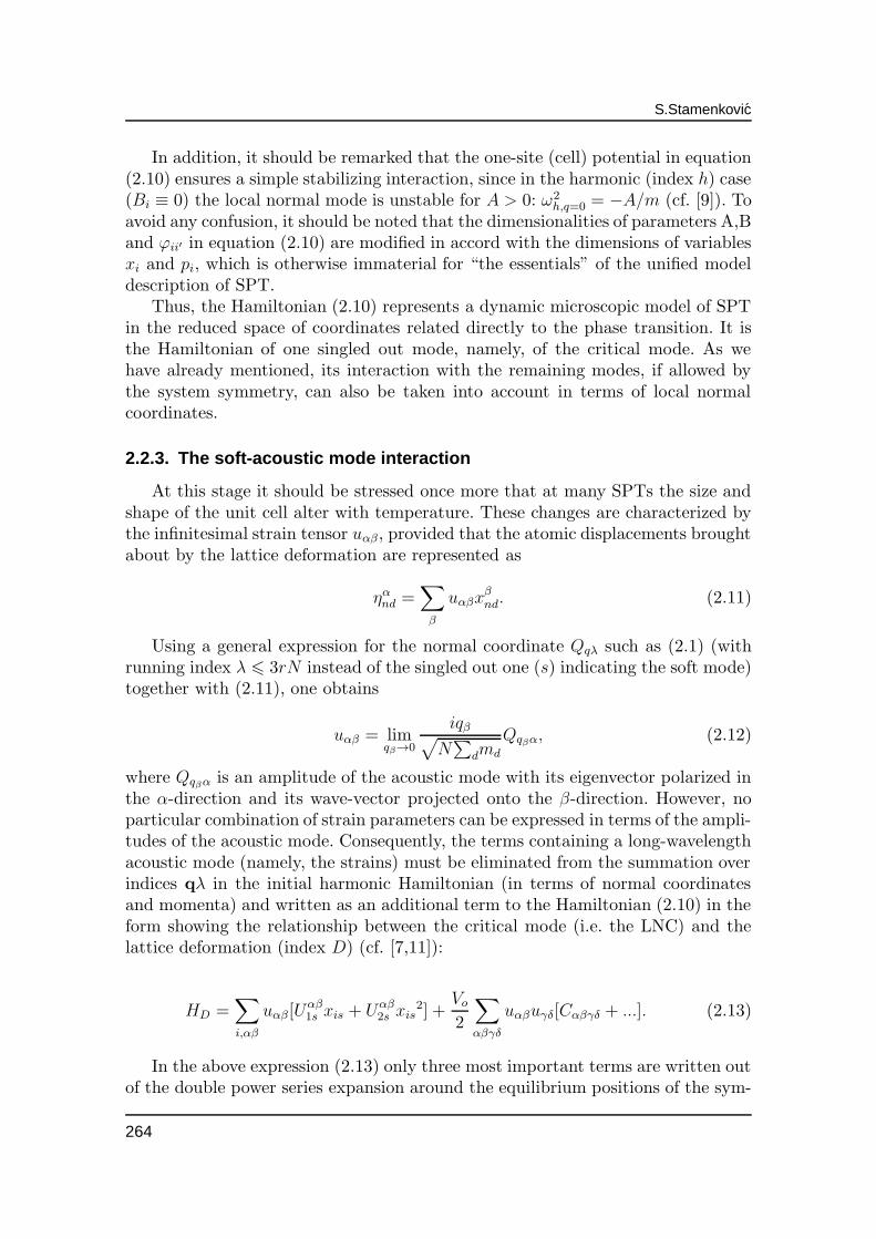
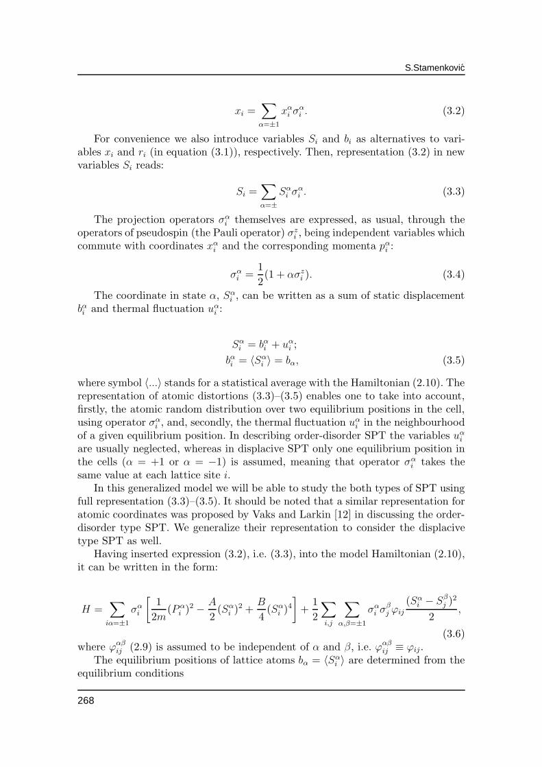
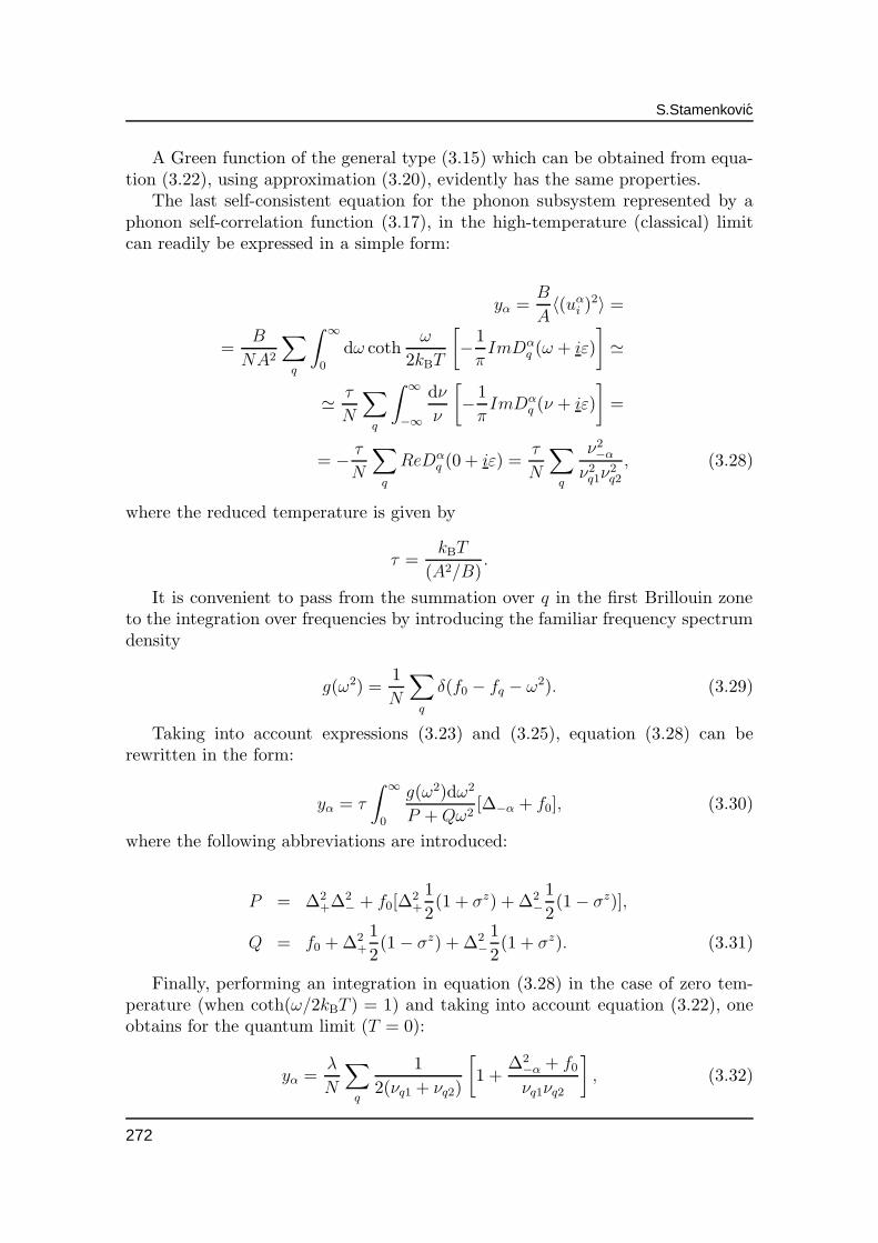
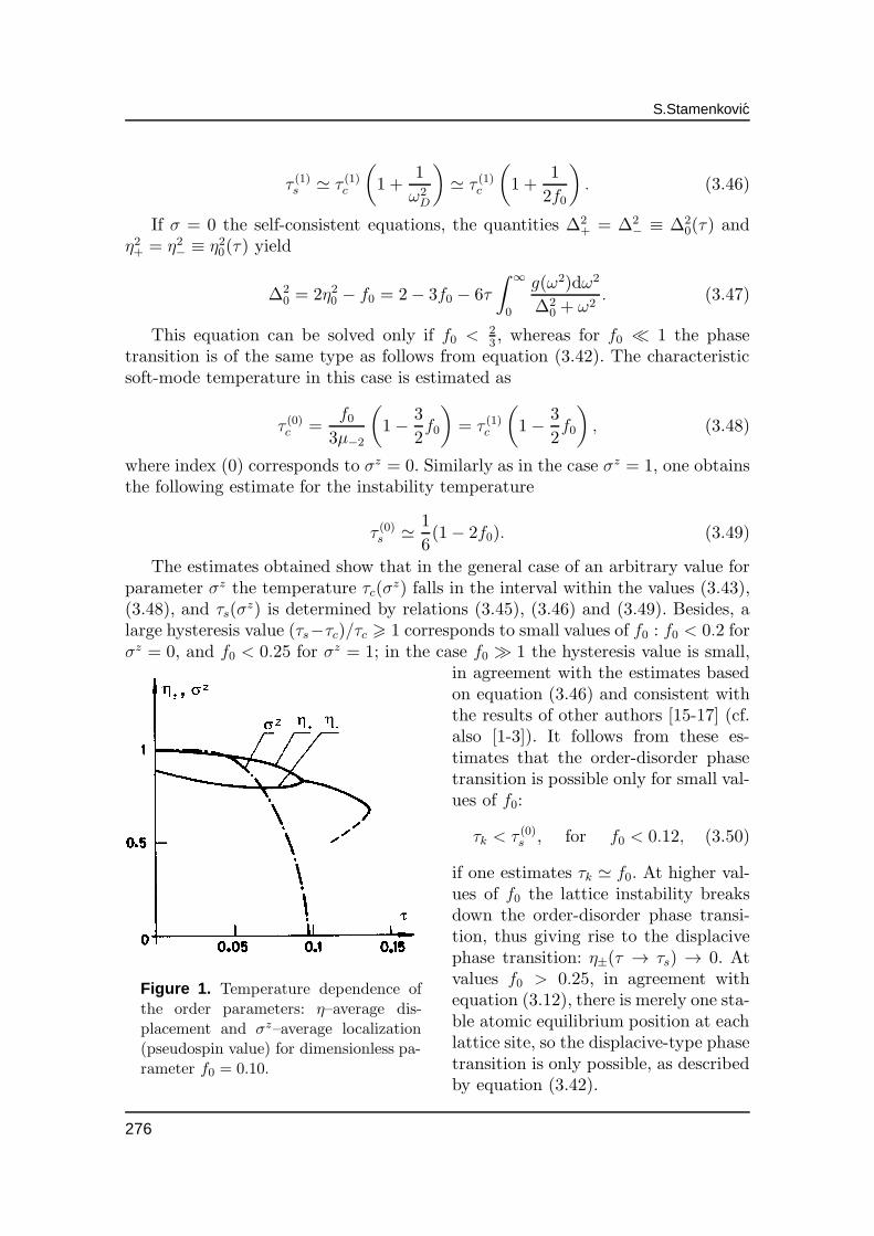
Figure 1. Temperature dependence ofthe order parameters: η–average dis-placement and σz–average localization(pseudospin value) for dimensionless pa-rameter f0 = 0.10.

in agreement with the estimates basedon equation (3.46) and consistent withthe results of other authors [15-17] (cf.also [1-3]). It follows from these es-timates that the order-disorder phasetransition is possible only for small val-ues of f0:

τk < τ (0)s , for f0 < 0.12, (3.50)

if one estimates τk ≃ f0. At higher val-ues of f0 the lattice instability breaksdown the order-disorder phase transi-tion, thus giving rise to the displacivephase transition: η±(τ → τs) → 0. Atvalues f0 > 0.25, in agreement withequation (3.12), there is merely one sta-ble atomic equilibrium position at eachlattice site, so the displacive-type phasetransition is only possible, as describedby equation (3.42).

276

Unified description of structural transitions

A mixed-type phase transition, as described by all the three order parametersη+(τ), η−(τ) and σ(τ), may be expected only in a very narrow region:

0.11 < f0 < 0.25. (3.51)

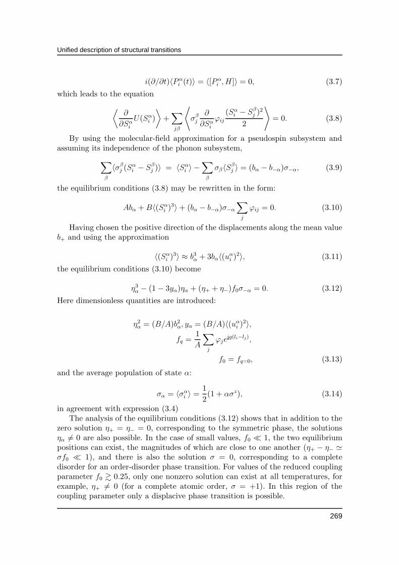
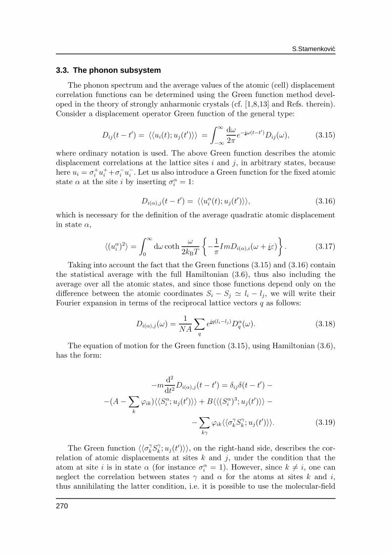
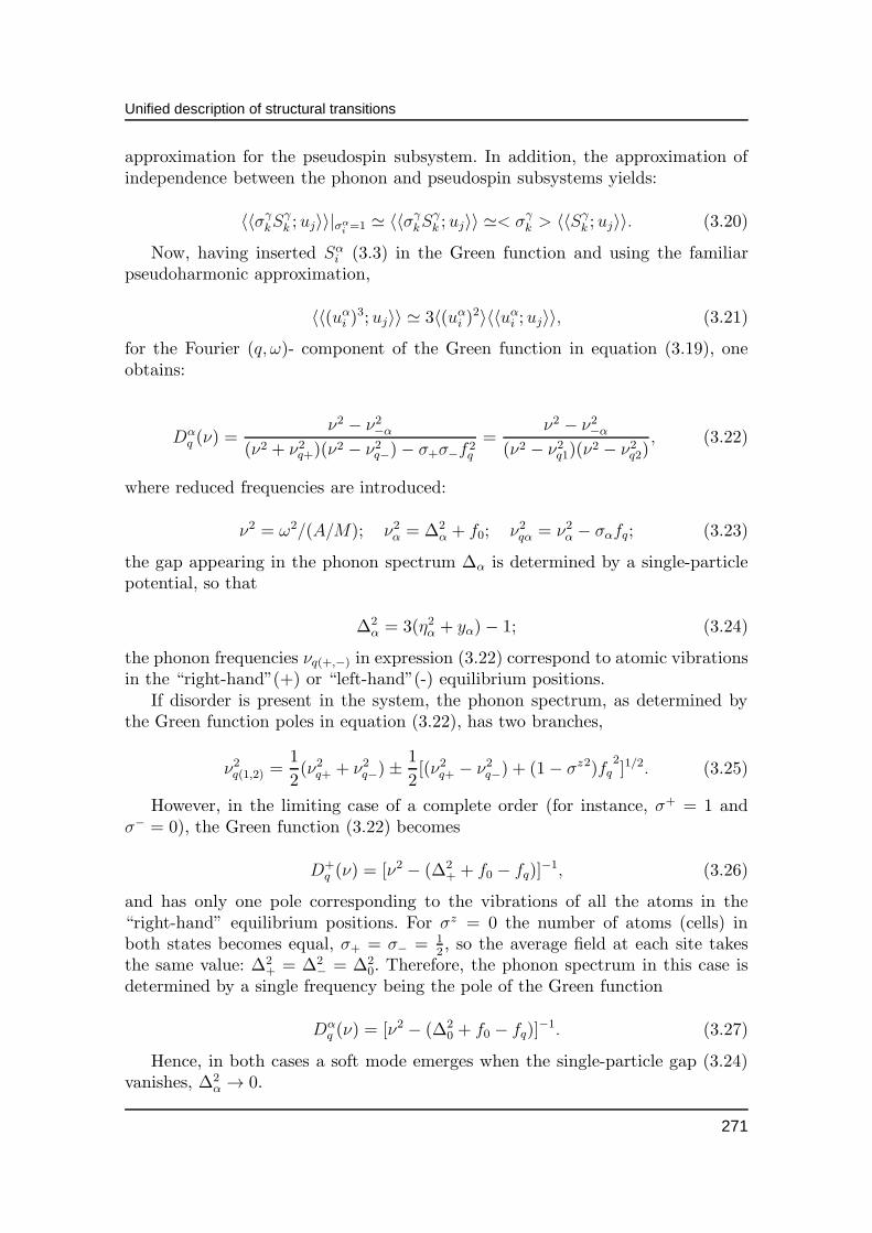
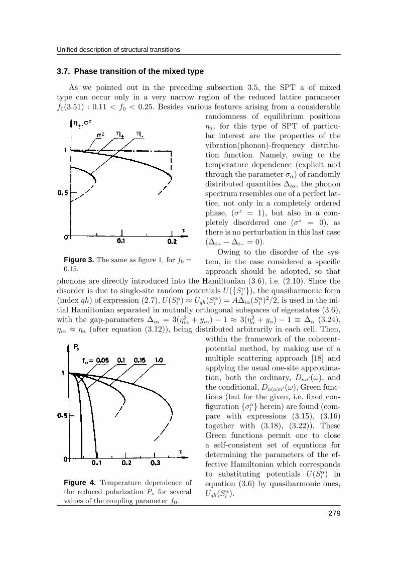
To confirm these general conclusions, the numerical solution of the self-consis-tent system of equations was obtained for the Debye model frequency spectrum(3.29), g(ω2) ∼ ω, ω < ωD, and the values of the coupling parameter f0 = 0.11, 0.12and 0.15 were taken. The numerical results for σz(τ) and η±(τ) are presentedin figures 1–3. It can be seen that the above estimates are in good agreementwith the numerical calculations. The temperature dependence of the spontaneouspolarization (3.41) for different f0 is shown in figure 4. Note, that in the regionof the order-disorder phase transition (f0 < 0.11), as compared with an ordinaryIsing model, the spontaneous polarization decreases more rapidly as temperatureincreases due to the temperature dependence of the effective exchange energy:J = f0A

2/4B(η+ + η−)2.

We note that these features are also obtained by slightly improved calculations[14] based on the coherent potential approximation developed for the systems withdisordered lattices (outlined hereafter in Subsection 3.7 for the case of mixed SPT).

3.6. The quantum limit in displacive SPT

In this section we will consider only two cases, namely, a completely ordered(σz = 1) lattice and a completely disordered (σz = 0) one [3]. It is assumed thatthe right choice of a transverse field Ω (within IMTF) or Glauber-like relaxationaldynamics ensure a transition from σz = 1 to σz = 0 at zero temperatures.

3.6.1. Displacive type phase transition in ordered lattice s

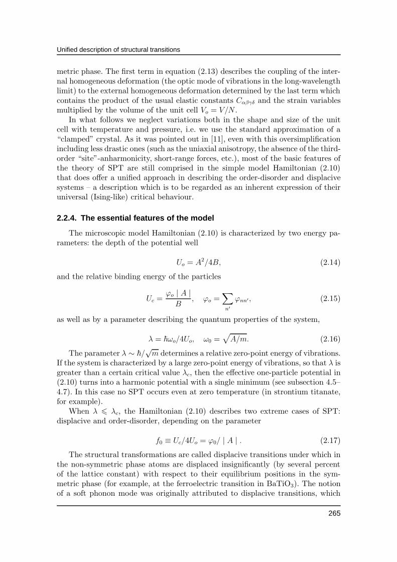
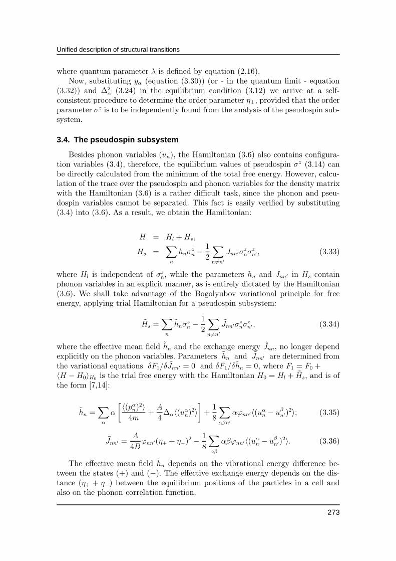
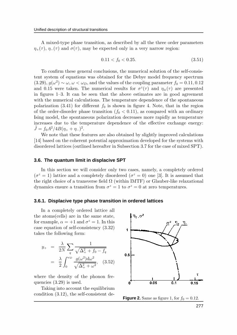
Figure 2. Same as figure 1, for f0 = 0.12.

In a completely ordered lattice allthe atoms(cells) are in the same state,for example, α = +1 and σz = 1. In thiscase equation of self-consistency (3.32)takes the following form:

y+ =λ

2N

∑

q

1√

∆2+ + f0 − fq

=λ

2

∫ ωD

0

g(ω2)dω2

√

∆2+ + ω2

, (3.52)

where the density of the phonon fre-quencies (3.29) is used.

Taking into account the equilibriumcondition (3.12), the self-consistent de-

277

S.Stamenkovic

termination of the equilibrium displacement η (or the gap in the frequency spec-trum ∆2

+ = 2η2) yields:

η2 = 1− 3

2λ

∫ ωD

0

g(ω2)dω2

√

2η2 + ω2. (3.53)

As it can be seen, the solution of this equation for η 6= 0 exists only if λ < λc(1),where the critical value λc(1) is determined by the expression:

λc(1) =2

3

[∫ ωD

0

g(ω2)dω2

ω2

]−1

=2

3

√f0

µ−1; (3.54)

here µ−1 = ω−1 is the average of the inverse frequency provided that for the Debyespectrum, g(ω2) = 3ω/ω3

D, µ−1 = 3/2√2 ≃ 1, if ω2

D = 2f0. Consequently, thedisplacive type transition in the ordered lattices can take place only if the latticeconsists of sufficiently heavy ions, that is if

m > mc =

(

2

3

√ϕ0

µ−1

A

B

)−2

, (3.55)

where the critical atomic (cell) mass (mc) is determined by model parameters (cf.also [15]).

3.6.2. Displacive type phase transition in disordered latt ices

Let us discuss the effect of disordering on the displacive type phase transition.By putting in equations (3.12) and (3.32) the value σz = 0 which corresponds toan equal number of atoms in the states α = ±1 (meaning that ∆2

+ = ∆2− ≡ ∆2

0,y+ = y− ≡ y and η+ = η− ≡ η), the following system of equations is then obtained:

η2 = 1− f0 − 3y, (3.56)

y =λ

2

∫ ωD

0

g(ω2)dω2

√

∆20 + ω2

. (3.57)

Therefore, a self-consistent equation for determining the gap ∆20 > 0 takes the

form:

∆20 = 2η2 − f0 = 2− 3f0 − 3λ

∫ ωD

0

g(ω2)dω2

√

∆20 + ω2

. (3.58)

Hence, the displacive type phase transition (η > 0) can take place if λ < λc(0),where the critical value λc(0) is determined by the condition ∆2

0(λc(0)) = 0, where-from

λc(0) =2

3

√f0

µ−1

(

1− 3

2f0

)

= λc(1)

(

1− 3

2f0

)

. (3.59)

Consequently, the occurence of the lattice disordering decreases both the limit-ing value of the allowed energy of zero-point fluctuations and the limiting value ofthe phase transition temperature (3.48). However, it has to be mentioned that thetransition into the state σz = 0 can take place if f0 ≪ 1, only when formula (3.59)is valid. In the case f0 > 1, only the state with σz = 1 is possible, and formula(3.54) holds.

278

Unified description of structural transitions

3.7. Phase transition of the mixed type

As we pointed out in the preceding subsection 3.5, the SPT a of mixedtype can occur only in a very narrow region of the reduced lattice parameterf0(3.51) : 0.11 < f0 < 0.25. Besides various features arising from a considerable

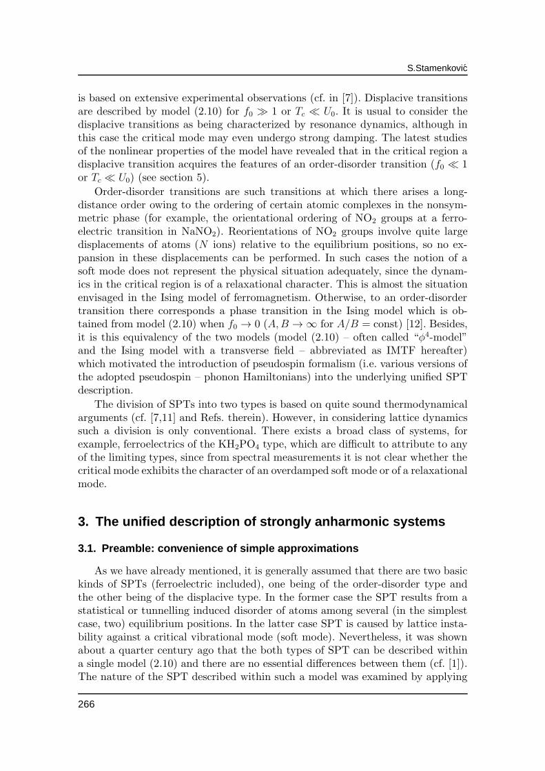
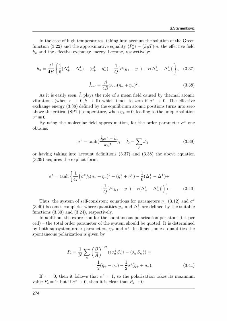
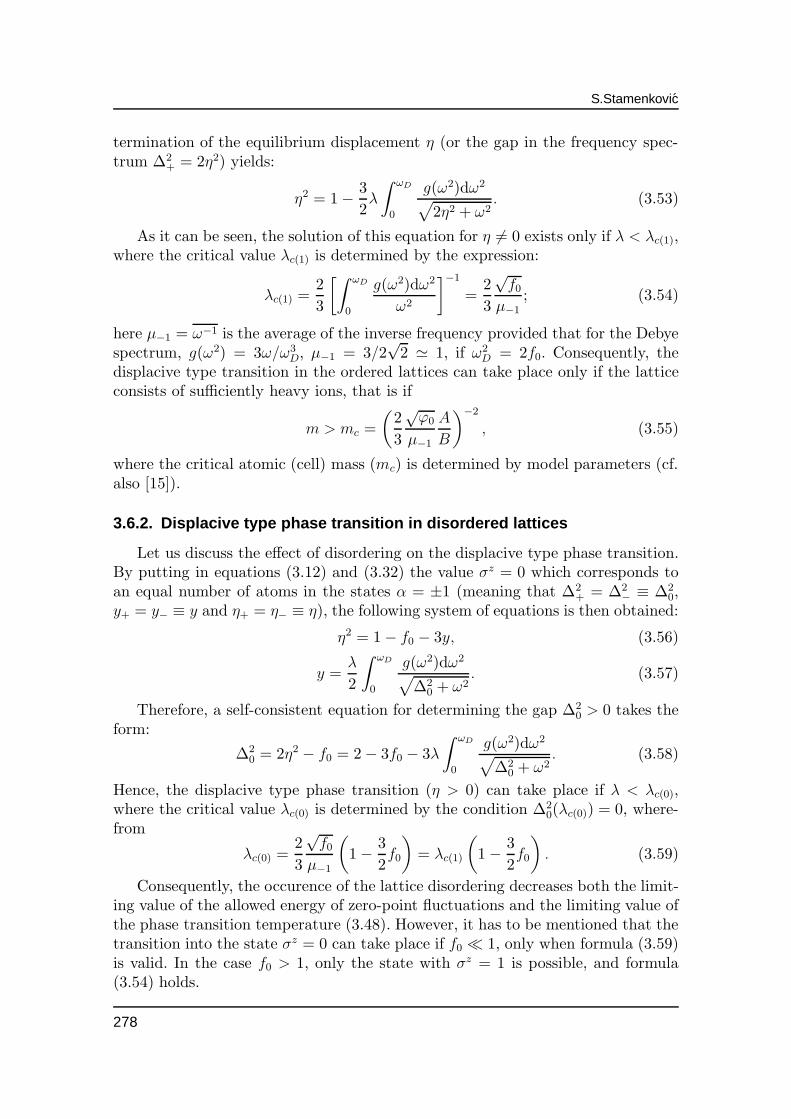
Figure 3. The same as figure 1, for f0 =0.15.

randomness of equilibrium positionsηn, for this type of SPT of particu-lar interest are the properties of thevibration(phonon)-frequency distribu-tion function. Namely, owing to thetemperature dependence (explicit andthrough the parameter σα) of randomlydistributed quantities ∆iα, the phononspectrum resembles one of a perfect lat-tice, not only in a completely orderedphase, (σz = 1), but also in a com-pletely disordered one (σz = 0), asthere is no perturbation in this last case(∆i+ −∆i− = 0).

Owing to the disorder of the sys-tem, in the case considered a specificapproach should be adopted, so that

phonons are directly introduced into the Hamiltonian (3.6), i.e. (2.10). Since thedisorder is due to single-site random potentials U(Sα

i ), the quasiharmonic form(index qh) of expression (2.7), U(Sα

i ) ≈ Uqh(Sαi ) = A∆iα(S

αi )

2/2, is used in the ini-tial Hamiltonian separated in mutually orthogonal subspaces of eigenstates (3.6),with the gap-parameters ∆iα = 3(η2iα + yiα) − 1 ≈ 3(η2α + yα) − 1 ≡ ∆α (3.24),ηiα ≈ ηα (after equation (3.12)), being distributed arbitrarily in each cell. Then,

Figure 4. Temperature dependence ofthe reduced polarization Ps for severalvalues of the coupling parameter f0.

within the framework of the coherent-potential method, by making use of amultiple scattering approach [18] andapplying the usual one-site approxima-tion, both the ordinary, Dnn′(ω), andthe conditional, Dn(α)n′(ω), Green func-tions (but for the given, i.e. fixed con-figuration σα

i herein) are found (com-pare with expressions (3.15), (3.16)together with (3.18), (3.22)). TheseGreen functions permit one to closea self-consistent set of equations fordetermining the parameters of the ef-fective Hamiltonian which correspondsto substituting potentials U(Sα

i ) inequation (3.6) by quasiharmonic ones,Uqh(S

αi ).

279

S.Stamenkovic

The explicit knowledge of the averaged over all configuration (index c) Greenfunctions 〈Dnn′(ω)〉c and 〈Dn(α)n′(ω)〉c, as expressed by their Fourier expansions inthe reciprocal lattice space, makes possible the calculation for the given values ofparameter σz of the lattice phonon spectrum:

ρ(ν2) = −(1/π)Im〈Dnn(ν + iε)〉c (3.60)

and of the phonon density of states for vibrations of an atom(cell) in a fixed stateα:

ρα(ν2) = −(1/π)Im〈Dn(α),n(ν + iε)〉c. (3.61)

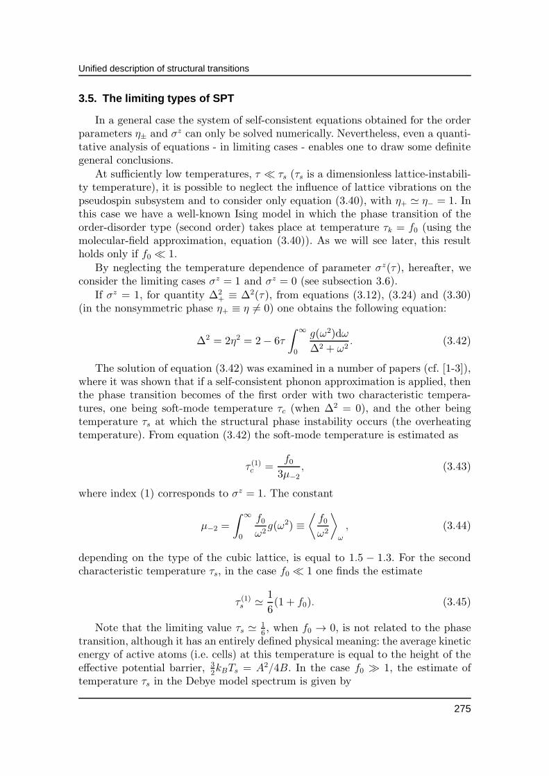
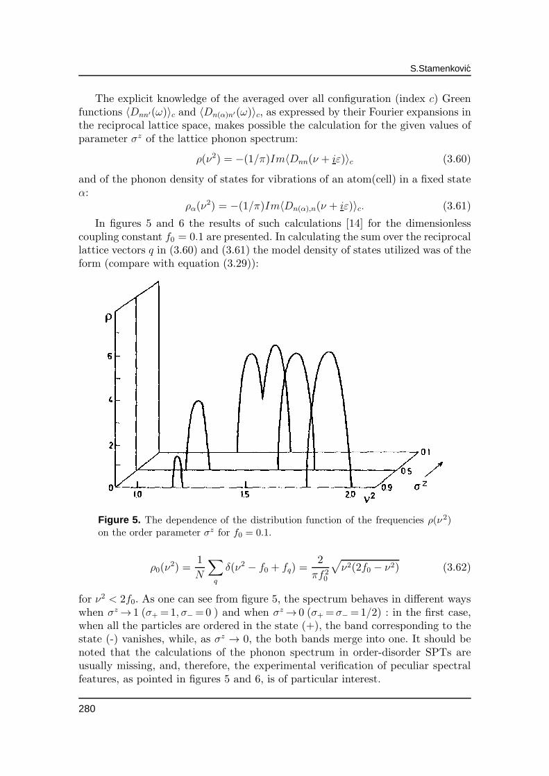
In figures 5 and 6 the results of such calculations [14] for the dimensionlesscoupling constant f0 = 0.1 are presented. In calculating the sum over the reciprocallattice vectors q in (3.60) and (3.61) the model density of states utilized was of theform (compare with equation (3.29)):

Figure 5. The dependence of the distribution function of the frequencies ρ(ν 2)on the order parameter σz for f0 = 0.1.

ρ0(ν2) =

1

N

∑

q

δ(ν2 − f0 + fq) =2

πf 20

√

ν2(2f0 − ν2) (3.62)

for ν2 < 2f0. As one can see from figure 5, the spectrum behaves in different wayswhen σz → 1 (σ+ =1, σ−=0 ) and when σz → 0 (σ+=σ− =1/2) : in the first case,when all the particles are ordered in the state (+), the band corresponding to thestate (-) vanishes, while, as σz → 0, the both bands merge into one. It should benoted that the calculations of the phonon spectrum in order-disorder SPTs areusually missing, and, therefore, the experimental verification of peculiar spectralfeatures, as pointed in figures 5 and 6, is of particular interest.

280

Unified description of structural transitions

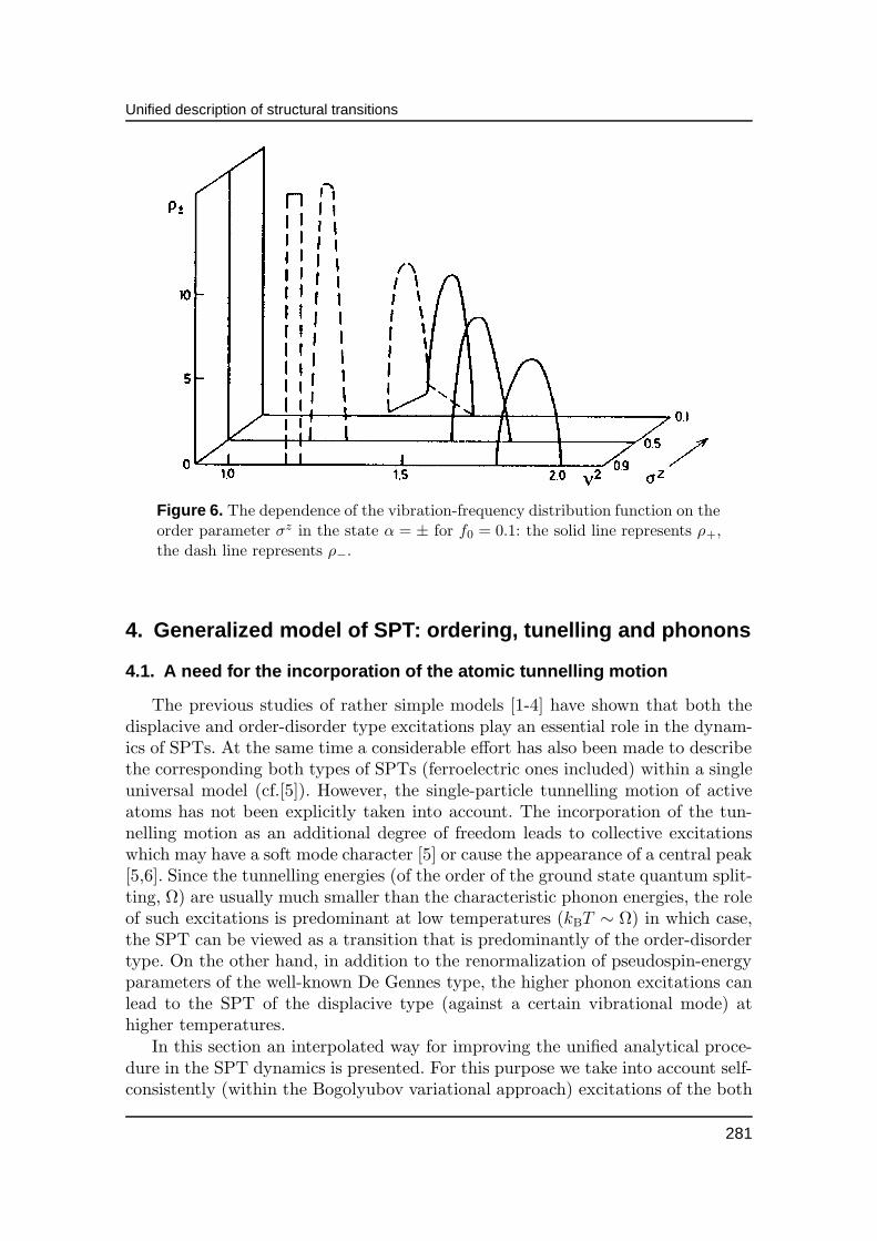
Figure 6. The dependence of the vibration-frequency distribution function on theorder parameter σz in the state α = ± for f0 = 0.1: the solid line represents ρ+,the dash line represents ρ−.

4. Generalized model of SPT: ordering, tunelling and phonon s

4.1. A need for the incorporation of the atomic tunnelling mo tion

The previous studies of rather simple models [1-4] have shown that both thedisplacive and order-disorder type excitations play an essential role in the dynam-ics of SPTs. At the same time a considerable effort has also been made to describethe corresponding both types of SPTs (ferroelectric ones included) within a singleuniversal model (cf.[5]). However, the single-particle tunnelling motion of activeatoms has not been explicitly taken into account. The incorporation of the tun-nelling motion as an additional degree of freedom leads to collective excitationswhich may have a soft mode character [5] or cause the appearance of a central peak[5,6]. Since the tunnelling energies (of the order of the ground state quantum split-ting, Ω) are usually much smaller than the characteristic phonon energies, the roleof such excitations is predominant at low temperatures (kBT ∼ Ω) in which case,the SPT can be viewed as a transition that is predominantly of the order-disordertype. On the other hand, in addition to the renormalization of pseudospin-energyparameters of the well-known De Gennes type, the higher phonon excitations canlead to the SPT of the displacive type (against a certain vibrational mode) athigher temperatures.

In this section an interpolated way for improving the unified analytical proce-dure in the SPT dynamics is presented. For this purpose we take into account self-consistently (within the Bogolyubov variational approach) excitations of the both

281

S.Stamenkovic

types (displacive and order-disorder) – in order to comprise both the tunnellingand higher phonon oscillations of active atoms (i.e. cells) within the framework ofa hybridized pseudospin-phonon model Hamiltonian separated in the correspond-ing variables. This is achieved by representing the cooperative atomic motion asa slow tunnelling process among several (in the simplest case, two) equilibriumpositions in addition to familiar phonon-like oscillations around some momentaryrest position. On the basis of the self-consistent phonon and molecular-field ap-proximations a complete system of coupled equations for two order parameters(average displacement η ∼ rsa and average localization σz) is obtained. Both qual-itative and detailed numerical analyses show that the SPT (of the first or secondorder) can be either of an order-disorder, a displacive or of a mixed type, depend-ing predominantly on the ratio of a two-particle potential to a single-particle oneand, in a lesser degree, on the ratio of the zero-point vibrational energy to theheight of a single-particle potential barrier. The possible SPT of the both typesat zero temperature (quantum limit), as well as the relation between these resultsand other relevant treatments are also discussed.

4.2. The model phonon-pseudospin Hamiltonian

Our previous [1,2] coordinate representation si =∑

α σiα(biα + uiα) (3.3) de-scribed the random atomic (cell) distribution (within the Ising model through theprojection operator σiα = 1/2(1+ασz

i )), over two (α=+,−) equilibrium positions(biα) at every site i, as well as thermal atomic fluctuations (uiα) around one or an-other momentary rest positions (biα) (“left” and “right” phonons) (see Subsection3.2). However, to elucidate more profoundly such an additional pseudospin degreeof freedom (σz

i ), one has to take into account the inherent quantum mechanicaleffect manifested in a single-particle tunnelling motion of active atoms inside some(real or effective) double-well potential, which was fully missing in our previousinvestigations and rather implicit in the approaches of other authors (cf. [1,2] andRefs. therein). For this purpose we suggested [4] the “left-right” representation ofthe model Hamiltonian (3.6) in the non-orthogonal pseudospin (i.e. “left”-“right”)basis. However, in accordance with the exhaustive analyses of many authors (cf.[5]), a clearer physical picture (and a rather transparent procedure) can be intro-duced by natural generalization of the traditional concept of atomic equilibriumstates. Thus, a time dependent local normal coordinate may be decomposed intoa slow tunnelling-like displacement (ri) and comparatively fast superimposed de-viations of the phonon type (ui) [5-7] (compare with (3.1)):

si = ri + ui; 〈ui〉 = 0. (4.1)

Such a representation holds under the “adiabatic” condition Ω ≪ ω0, ω0, being acharacteristic frequency of lattice vibrations.

Having inserted definition (4.1) into the general Hamiltonian (2.4) (assumingone-component coordinate Ri ≡ xi and momentum Pi = −i~ ∂

∂Ri≡ −i~ ∂

∂xi) it can

be written in a trial form separated in the corresponding variables:

282

Unified description of structural transitions

H0 = Hph(ui) +Ht(ri), (4.2)

where the phonon-like (index ph) and tunnelling-like (index t) Hamiltonians aregiven by

Hph =∑

i

P 2i

2m+

1

2

∑

ij

φijuiuj, (4.3)

Ht =∑

i

[

p2i2m

+ U(ri)

]

+1

2

∑

i 6=j

Cij(ri − rj)2; (4.4)

φij, Cij and U(ri) are variational parameters and Pi and pi – canonical conjugatemomenta to ui and ri, respectively. For a strongly anharmonic motion described byequation (4.4) it is convenient to introduce the energy representation comprisingsingle-particle ground doublet (symmetric (ψs) and antisymmetric (ψa)) stateswhich satisfy the eigenvalue equation:

[

P 2i

2m+ U(ri)

]

ψs,a(ri) = εs,aψs,a(ri). (4.5)

Going over to the pseudospin representation, Ht (4.4) is presented in the well-known De Gennes form (e.g. IMTF) (cf. [5]):

Hs = −Ω∑

i

σxi −

1

2

∑

i

Jijσzi σ

zi +E0 , (4.6)

where the energy parameters Ω, Jij and Eo are simple functions of εα, Cij, and thematrix elements rαβ = 〈α | ri |β〉 and r2αα = 〈α | r2i |α〉 (α, β = s, a) calculated withthe wave functions ψα in equation (4.5):

Ω =1

2(εa − εs) + r2−C0,

E0 =1

2(εa + εs) + r2+C0,

Jij = 2r2saCij;

r2± =1

2(r2aa ± r2ss);

C0 =∑

j

Cij . (4.7)

The variational parameters φij, Cij and U(ri) are determined from the Bo-golyubov variational principle for the free energy of system F , namely, from thecondition of stationarity of free energy:

F1 = F0 + 〈H −H0〉0 > F, (4.8)

283

S.Stamenkovic

with respect to variations over these parameters or, equivalently, over the cor-responding correlation functions (cf. [8]). In the above expression (4.8) symbol< ... >0 stands for the statistical averaging with the trial Hamiltonian H0 ((4.2)–(4.7)), to which free energy F0 corresponds.

Computing free energy F1 (4.8) where

F0 = −kBT ln Spe−H0/T, (4.9)

〈H −H0〉0 = SpeF0−H0

T (H −H0) =

=∑

i

〈U(ri + ui)〉0 +1

2

∑

ij

〈V (ri + ui, rj + uj)〉0 −

−∑

i

〈U(ri)〉0 −1

2

∑

ij

φij〈uiuj〉0 −1

2

∑

ij

Cij〈(ri − rj)2〉0 (4.10)

under the assumption that condition 〈Pipi〉0 = 0 holds, for the variational param-eters of the trial Hamiltonians (4.3) and (4.4) (i.e. (4.6)) the following equationsare obtained:

φij =δ

δ〈uiuj〉02

∑

i

〈U(ri + ui)〉0 +∑

i 6=j

〈V (ri + ui, rj + uj)〉0, (4.11)

2r2saCij =δ

δ〈σzi σ

zi 〉0

〈V (ri + ui, rj + uj)〉0, (4.12)

and

δ

δ〈σxi 〉0

∑

i

〈U(ri)〉0 =δ

δ < σxi >0

∑

i

〈U(ri + ui)〉0 +

+1

2

∑

ij

〈V (ri + ui, rj + uj)〉0 −1

2

∑

ij

Cij〈r2i + r2j 〉0. (4.13)

The self-consistent system of equations (4.3)–(4.7), (4.11)-(4.13) determinesthe phase transition of the model and describes the mutual influence of phononand pseudospin subsystems if the potentials U(si) and V (si, sj) in equation (2.4)are appropriately modelled.

4.3. The structural phase transition in the model

Having chosen a single-particle double-well potential U(si) in the convenientform (2.7) and a pair-potential V (si, sj) in the familiar harmonic approximation(2.8), we assume the model Hamiltonian of the system in the previous form (2.10):

284

Unified description of structural transitions

H =∑

i

(

− ~2

2m

∂2

∂s2i− A

2s2i +

B

4s4i

)

+1

4

∑

ij

ϕij(si − sj)2. (4.14)

The variational approach for this Hamiltonian yields:

φij = δij(A∆+ ϕ0)− ϕij(1− δij); 2Cij = ϕij, ϕ0 =∑

j

ϕij , (4.15)

where

∆ = 3(B/A) < r2i >0 − a , a = 1− 3(B/A)〈u2i 〉 . (4.16)

The effective (renormalised) single-particle (cell) potential in (4.4) can be writ-ten in the form:

U(ri) = −A2r2i +

B

4r4i ; A = A− 3B〈u2i 〉0 ≡ Aa . (4.17)

The self-correlation displacement functions relevant to the nature of the SPTare determined by the following approximative equations (of the RPA type):

〈u2i 〉0 =1

Nm

∑

k

1

2ωk

cothωk

2kBT, (4.18)

〈r2i 〉0 =1

2[(r2ss + r2aa) + (r2ss − r2aa) + (r2ss + r2aa)〈σx

i 〉0], (4.19)

where the phonon frequency ωk is given by the equation

mω2k = A∆+ ϕ0 − ϕk; ϕk =

∑

j

ϕijeik(li−lj). (4.20)

In the mean(molecular)-field approximation (equivalent to RPA for pseudospins)(see, e.g., [19]) one obtains:

〈σx,zi 〉 = σx,z =

hx,zh

tanhh

kBT;

hx = Ω, hz = J0σz, h2 = h2x + h2z; J0 =

∑

j

Jij = r2saϕ0 . (4.21)

Thus, the SPT-system is described by the solution of the above self-consistentsystem of equations which, owing to equation (4.5), can be obtained only numeri-cally. Nevertheless, a qualitative analysis for the limiting cases is possible.

285

S.Stamenkovic

a) Order-disorder transition

Analogously to the analysis in the previous sections, in the weak coupling limitof small ϕ0, i.e. in the temperature region when

ϕ0 ≪ A = A− 3B〈u2i 〉0, (4.22)

the order-disorder transition is possible in the pseudospin subsystem as charac-terized by the order parameter σz. In the molecular field approximation for theorder-disorder transition temperature Tc one finds:

Tc ≃ J02q

ln 1+q1−q

; q = Ω/J0 ≤ 1. (4.23)

The estimates obtained in the case of weak tunnelling (Ω ≪ J0; r2ss ∼ r2aa ∼

r2sa ∼ r20 = A/B) correspond to the results of section 3 (for f0 ≪ 1, therein),namely,

Tc ∼ J0 ∼ ϕ0r20 ∼ ϕ0

A

B≪ U0. (4.24)

Note that phonon excitations do not play an essential role in this case, since〈u2i 〉0 ≪ r20.

b) Displacive transition

When the temperature is raised, the atomic fluctuations 〈u2i 〉0 cannot be ne-

glected and the character of the coupling could be changed, i.e. ϕ0 ≫ A (even forϕ0 ≪ A), thus, leading to the displacive phase transition: ∆(T0) → 0 and r20(T0) →0. In the classical limit of high temperatures (T & T0>Tc) [1-7],

A(T0) = 0, 〈u2i 〉0 =1

3

A

B, (4.25)

while in the strong-coupling limit 〈u2i 〉 ∼ T/mω20 ∼ T/ϕ0 also holds and the dis-

placive transition temperature is estimated as

T0 ∼1

3ϕ0(A/B), (4.26)

provided that for the model considered the inequality Tc ∼ ϕ0A/B < T0 ∼ ϕ0A/Bis constantly valid. For both limiting types of SPTs the similar results have beenobtained in subsection 3.5.

4.4. Approximation of a double well by two truncated harmoni c oscillators

For the trial wave functions in equation (4.5) one can assume the linear com-binations of the ground states, ψ−

0 and ψ+0 , referred to the “left” (-) and “right”

(+) unperturbed harmonic oscillators, respectively, to be of the form:

286

Unified description of structural transitions

ψs,a = [2(1± ρ)]−1/2[ψ+0 (r)± ψ−

0 (r)] , (4.27)

where

ψ±0 (r) = ψ0(r ± r0) ; ψ0(r) = (a0

√π)−1/2 exp(−r2/2a20) ;

a20 = ~/mω ; ω2 = k/m , r0 = (A/B)1/2 . (4.28)

Here ρ is the overlap integral of the “left” and “right” states; the harmonic force-constant k = 2A is renormalised to be k = 2A (in the approximation of a strongparticle (i.e. cell) localization). By performing the corresponding calculations onefinds:

ρ =

∫

ψ+0 (r)ψ

−0 (r)dr = exp−A

2/B

ω/2 = exp(−1/λ) ; (4.29)

λ =ω

2A2/B= a20/r

20 =

λ0√2(1− 3y)3/2

, (4.30)

where the temperature independent quantum parameter (compare with equation(2.16)) characterizing the zero-point vibrations λ0 = ~ω0/(A

2/B), ω0 =√

A/m isintroduced, and parameter y = (B/A)〈u2i〉 is the reduced average quadratic “fast”displacement ( after equation (4.18)). Consequently, for the parameters of thepseudospin Hamiltonian (4.6) the following expressions are obtained:

Ω =A2

4√2B

λ0ρ√1− 3y

1− ρ2(1 +

3

λ) , (4.31)

r2sa = r20/(1− ρ2); r20 = (A/B)(1− 3y) , (4.32)

r2ss =r20

1± ρ

[

1 +λ

2(1± ρ)

]

, (4.33)

where the reduced average quadratic “slow” displacement (4.19) becomes

r ≡ B

A〈r2i 〉0 =

1− 3y

1− ρ2

[

1 +λ(1− ρ2)

2− ρσx

]

. (4.34)

To make explicit the reduced average quadratic “fast” displacement (4.18), thespectral density of phonon frequencies is introduced:

g(ν) =2

π

√1− ν2; ν =

ω

A/m, (4.35)

and then one finds

y = λ0

∫ 1

−1

dνg(ν)

2√∆− f0ν

cothλ0√∆− f0ν

2θ, f0 = ϕ0/A; θ =

kBT

A2/B, (4.36)

where

287

S.Stamenkovic

∆ = 3(y + r)− 1 , (4.37)

is a gap in the phonon spectrum (4.20).Finally, owing to equation (4.32), the spontaneous polarization (per cell) of

the system is simply expressed as a product of the displacive-like (η) and theorder–disorder-like (σz) order parameters:

Ps =1

N

∑

i

(B

A)1/2〈ri〉0 =

(

B

A

)1/2

rsaσz = ησz , (4.38)

where the order parameters σz and η are given by the above self-consistent proce-dure: σz – by equation (4.21) and η ≡ (B/A)1/2rsa – by the expression

η =

1− 3y

1− ρ2

1/2

. (4.39)

Both the “order-disorder” (σz) and the “displacive” (η) order parameters areto be found as a self-consistent solution of equations (4.21), (4.29)-(4.37). For agiven set of the reduced energy parameters (λ0, f0) the competition of these orderparameters determines the character of the SPT.

4.5. The quantum limit of zero temperature

At zero temperature equations (4.21) and (4.36) become

σz =1

J0

√

J20 − Ω2 , σx =

Ω

Jo; (4.40)

y = λ0

∫ 1

−1

dν√1− ν2

π√∆− f0ν

. (4.41)

As it is easily seen from equation (4.40), σz > 0 if Ω 6 J0. Using equation(4.41) with equations (4.21), (4.32), one obtains the condition for λ0,

ρc4f0

(3 + λ0)(1− 3yc) = 1 , (4.42)

which defines the maximum λ0(λc0) at which σ

z > 0 is still possible. In a simplifiedcase, when yc ≪ 1

3, the graphical solution of equation (4.42) gives

λc0 ≃ 1/ ln[(3/4)f0]. (4.43)

Hence, if λ0 > λc0, then σz = 0, even at zero temperature.

The order parameter η can also vanish at zero temperature. Using equations(4.36), (4.37) and (4.39), one obtains

λph0 ≃ 2√

f0. (4.44)

288

Unified description of structural transitions

In such a way the zero-point vibrations can destroy the ordered ground stateat T =0 K, both in the pseudospin and the phonon subsystems. One can expectthat Ps vanishes either in σz or in η, depending on the competition between λc

0

and λph0 , i.e. on the lesser of the two. The corresponding estimates of λc0 and λph0

for various values of parameter f0 are given in table I.

TABLE If0 0.05 0.10 0.30 0.50λc0 0.37 0.50 1.95 2.50

λph0 0.44 0.62 1.10 1.40

4.6. The numerical results

4.6.1. The case of the double-well potential modelled by two harmonic os-cillators

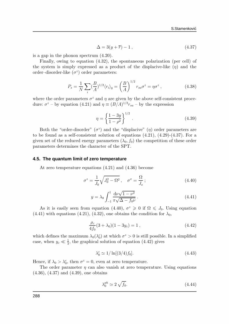
Figure 7. The order parameters sigmaz andη, the polarization Ps and the overlapping pa-rameter ρ as functions of temperature (θ). Pa-rameters σz, η, Ps–upon θ-scale and ρ–uponabove-scaled θ-abscissa correspond to λ0 =0.5 and f0 = 0.5; the marked parameters σz

I ,ηI , P

Is , etc., upon θI -scale, etc., correspond to

λ0 = 0.1 and various f0 = 0.1, 0.2, 0.6, respec-tively.

The system of self-consistentequations (4.21) and (4.29)–(4.39) is solved numerically andσz(θ), η(θ), Ps(θ) (for various f0and λ0) and ρ(θ) (for f0 = λ0 =0.5 as well as σz(λ0), η(λ0) (forf0 = 0.6 and θ = 0.001) and ρ(λ0)(for various f0 = 0.1, 0.2, 0.6 andθ = 0.001) are presented in fig-ures 7 and 8, respectively [5]. Itcan be observed that the quali-tative estimates in the precedingsubsections (4.3–4.5) are in goodagreement with the numerical cal-culations. For all marked param-eters (I to III) the overlapping in-tegral ρ, as calculated, is of the or-der 0.003 at T ≃ TSPT . The corre-sponding curves in figure 7 are inagreement with our previous ones[1] (cf. section 3). In the weak-coupling limit f0 = f 1

0 /(1−f 10 ) ≪

1 (f 10 being the reduced coupling

constant f0 in [1], i.e. in equa-tion (3.13)), the proper accountof tunnelling effects is taken forρ ≪ 1 (at least ρ < 0.5 andλ0 < 0.5), in agreement with theprevious results for both the order

parameter (here η) and the exact curves for σz [15].

289

S.Stamenkovic

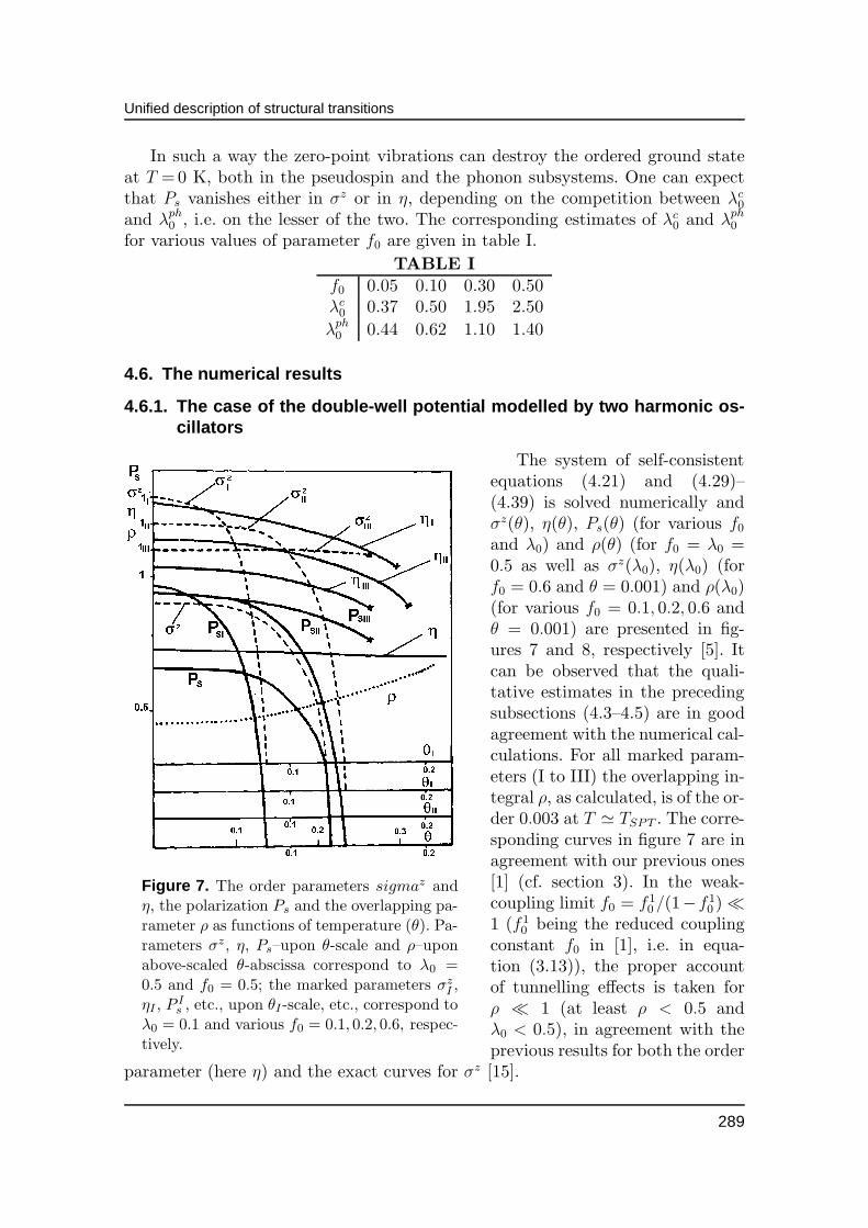
Figure 8. The order parameters σz,η and the overlapping parameter ρ asfunctions of the quantum parameter λ0.σz and η are presented for f0 = 0.6;ρ1, ρ2, ρ3 correspond to various f0 =0.1, 0.6, 1.0, respectively.

The appearance of imaginary solu-tions in both figures, 7 and 8, is as-signed by cross-points. A discontinuityitself in the displacive SPT (but in thecase f0 ≪ 1) is a well-known character-istic of the self-consistent phonon ap-proximation (cf. [1,7]). In the strong-coupling limit (f0 ≫ 1) (when thetunnelling can be disregarded) the dis-placive SPT does occur and is properlydescribed as previously [1]. As it can beobserved in figure 7, the case “III”(f0 =0.6) corresponds to a mixed SPT. In fig-ure 8 η(λ0) has a minimum indicated as

λph(1)0 ; λ

ph(2)0 denotes a value at which η

becomes imaginary and λc0 is a critical

λ0 for the pseudospin subsystem (forλ0 > λc0, σ

z = 0).

4.6.2. The exact results based on the model of quartic oscill ator

The self-consistent numerical calculations using the renormalized double-wellpotential (4.17) are also performed, provided that the overlap of the exact (indexexc) wave functions ψs and ψa, ρexc = 〈s | a〉exc, is now equal to zero [5]. Thedependence of all the relevant parameters for various f0, λ0 and temperaturesfairly agrees with the numerical calculations (using trial doublet states) whenρ < 0.5 (figures 7 and 8). As an illustration, only some truncated results forthe dimensionless parameters are presented in tables II and III. As an indicativecorollary we also note that for θ close to zero an appreciable λ0 – dependence ofall the parameters is found, while the f0 – dependence of these parameters (exceptfor J0) can be ignored (cl.[5]).

TABLE IIλ0 = 0.1; f0 = 0.1θ Ω 10−3 J0 η y σz σx Ps

0.020 0.190 0.075 0.866 0.041 0.999 0.002 0.8650.040 0.220 0.074 0.858 0.045 0.939 0.003 0.8050.060 0.320 0.070 0.837 0.056 0.617 0.004 0.5160.080 0.530 0.064 0.803 0.072 0.1 · 10−6 0.006 0.8 · 10−7

0.100 0.110 0.055 0.744 0.098 0.1 · 10−6 0.011 0.8 · 10−7

290

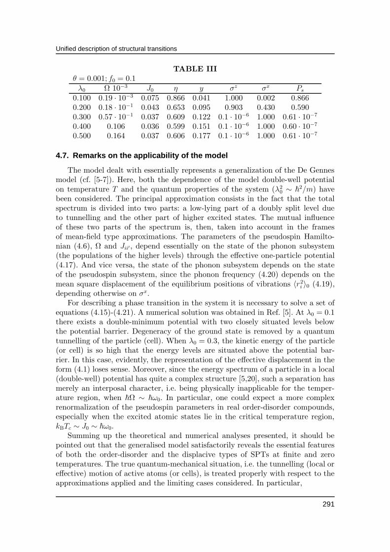
Unified description of structural transitions

TABLE IIIθ = 0.001; f0 = 0.1λ0 Ω 10−3 J0 η y σz σx Ps

0.100 0.19 · 10−3 0.075 0.866 0.041 1.000 0.002 0.8660.200 0.18 · 10−1 0.043 0.653 0.095 0.903 0.430 0.5900.300 0.57 · 10−1 0.037 0.609 0.122 0.1 · 10−6 1.000 0.61 · 10−7

0.400 0.106 0.036 0.599 0.151 0.1 · 10−6 1.000 0.60 · 10−7

0.500 0.164 0.037 0.606 0.177 0.1 · 10−6 1.000 0.61 · 10−7

4.7. Remarks on the applicability of the model

The model dealt with essentially represents a generalization of the De Gennesmodel (cf. [5-7]). Here, both the dependence of the model double-well potentialon temperature T and the quantum properties of the system (λ2

0 ∼ ~2/m) have

been considered. The principal approximation consists in the fact that the totalspectrum is divided into two parts: a low-lying part of a doubly split level dueto tunnelling and the other part of higher excited states. The mutual influenceof these two parts of the spectrum is, then, taken into account in the framesof mean-field type approximations. The parameters of the pseudospin Hamilto-nian (4.6), Ω and Jii′, depend essentially on the state of the phonon subsystem(the populations of the higher levels) through the effective one-particle potential(4.17). And vice versa, the state of the phonon subsystem depends on the stateof the pseudospin subsystem, since the phonon frequency (4.20) depends on themean square displacement of the equilibrium positions of vibrations 〈r2i 〉0 (4.19),depending otherwise on σx.

For describing a phase transition in the system it is necessary to solve a set ofequations (4.15)-(4.21). A numerical solution was obtained in Ref. [5]. At λ0 = 0.1there exists a double-minimum potential with two closely situated levels belowthe potential barrier. Degeneracy of the ground state is removed by a quantumtunnelling of the particle (cell). When λ0 = 0.3, the kinetic energy of the particle(or cell) is so high that the energy levels are situated above the potential bar-rier. In this case, evidently, the representation of the effective displacement in theform (4.1) loses sense. Moreover, since the energy spectrum of a particle in a local(double-well) potential has quite a complex structure [5,20], such a separation hasmerely an interposal character, i.e. being physically inapplicable for the temper-ature region, when ~Ω ∼ ~ω0. In particular, one could expect a more complexrenormalization of the pseudospin parameters in real order-disorder compounds,especially when the excited atomic states lie in the critical temperature region,kBTc ∼ J0 ∼ ~ω0.

Summing up the theoretical and numerical analyses presented, it should bepointed out that the generalised model satisfactorily reveals the essential featuresof both the order-disorder and the displacive types of SPTs at finite and zerotemperatures. The true quantum-mechanical situation, i.e. the tunnelling (local oreffective) motion of active atoms (or cells), is treated properly with respect to theapproximations applied and the limiting cases considered. In particular,

291

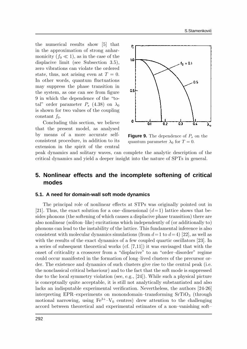
S.Stamenkovic

Figure 9. The dependence of Ps on thequantum parameter λ0 for T = 0.

the numerical results show [5] thatin the approximation of strong anhar-monicity (f0 ≪ 1), as in the case of thedisplacive limit (see Subsection 3.5),zero vibrations can violate the orderedstate, thus, not arising even at T = 0.In other words, quantum fluctuationsmay suppress the phase transition inthe system, as one can see from figure9 in which the dependence of the “to-tal” order parameter Ps (4.38) on λ0is shown for two values of the couplingconstant f0.

Concluding this section, we believethat the present model, as analysedby means of a more accurate self-consistent procedure, in addition to itsextension in the spirit of the centralpeak dynamics and solitary waves, can complete the analytic description of thecritical dynamics and yield a deeper insight into the nature of SPTs in general.

5. Nonlinear effects and the incomplete softening of critic almodes

5.1. A need for domain-wall soft mode dynamics

The principal role of nonlinear effects at STPs was originally pointed out in[21]. Thus, the exact solution for a one–dimensional (d=1) lattice shows that be-sides phonons (the softening of which causes a displacive phase transition) there arealso nonlinear (soliton–like) excitations which independently of (or additionally to)phonons can lead to the instability of the lattice. This fundamental inference is alsoconsistent with molecular dynamics simulations (from d=1 to d=4) [22], as well aswith the results of the exact dynamics of a few coupled quartic oscillators [23]. Ina series of subsequent theoretical works (cf. [7,11]) it was envisaged that with theonset of criticality a crossover from a “displacive” to an “order–disorder” regimecould occur manifested in the formation of long–lived clusters of the precursor or-der. The existence and dynamics of such clusters give rise to the central peak (i.e.the nonclassical critical behaviour) and to the fact that the soft mode is suppresseddue to the local symmetry violation (see, e.g., [24]). While such a physical pictureis conceptually quite acceptable, it is still not analytically substantiated and alsolacks an indisputable experimental verification. Nevertheless, the authors [24-26]interpreting EPR–experiments on monondomain–transforming SrTiO3 (throughmotional narrowing, using Fe3+–V0 centres) drew attention to the challengingaccord between theoretical and experimental estimates of a non–vanishing soft–

292

Unified description of structural transitions

mode frequency at the phase transition temperature (Tc), thus, prompting furtherprogress in comprehensive SPT investigations. Apparently, such a coincidence cor-roborates the model description [1-5,21-26] by which the local normal coordinatesi(t) is decomposed into a slow momentary quasirest position (ri(t)) and a com-paratively fast deviation ui(t) (around ri(t)) of the phonon (quasiharmonic) type.In the frames of such ideas, our preceding works [1-5,7] were devoted to analyticalstudies of the SPT description within a single universal model, using in additionthe Bogolyubov variational approach. Thus, a novel interpolar scheme attemptingto include all the intriguing features of the SPT, i.e. statistical order–disorder,tunnelling (real and effective) and phonon excitations has been proposed (see Sec-tion 3 and 4). To describe a possible order–disorder behaviour of the traditionallydisplacive SPT (revealed in an incomplete phonon softening) the adjustment ofthe previous models is accomplished by employing both the solitary–waves andrenormalization–group (RG) techniques (cf. [5-7]). Note that the RG–method hasbeen used in this sense only for order–disorder systems [27].

5.2. The critical region

The unified theory of SPTs afforded by the model studies which were surveyedin the preceding sections can be qualified as applicable within the same limitsas the Landau theory. Such a description provides a qualitative picture of SPTs,particularly of traditionally limiting types, as well as for some model parametersof mixed transitions which do not belong to either of two extreme cases. However,like the previous theories, it does not permit investigation of their properties inthe critical region (cf. also [7,11]).

Investigation of the phase transition (for instance, in strontium titanateSrTiO3, with the aid of inelastic neutron scattering (cf. [7])) reveals that theexcitation spectrum in the critical region is more complex than that which fol-lows from the classical theory. The scattering intensity exhibits, besides two sidepeaks corresponding to the soft mode, a narrow peak at zeroth energy transfer.As T → Tc the intensity of this central peak increases sharply, while its widthdecreases. The frequency of the soft mode decreases up to a certain finite value atT =Tc. Subsequent experiments demonstrate that this pattern is characteristic ofall SPTs.

At present the nature of the central peak still remains to be clarified. Thereasons for its appearance are divided into two sorts: intrinsic (fluctuations of thephonon density, nonlinear effects, etc.) and extrinsic (defects, impurities, surface).The results of numerous studies of this question, as well as an extensive bibliogra-phy, can be found in the reviews (cf. [7,11]). It can be concluded from the resultsof these works that a system in the critical region is characterized by two timescales, instead of one, as in the conventional theory of the soft mode. In additionto the relatively short (noncritical) relaxation time of the system characterizingthe soft phonon, there exists a large (critical) relaxation time characterizing thenarrow central peak. In this section, on the basis of model (2.10), the rise of adouble-time evolution at a displacive or an order-disorder phase transition in a

293

S.Stamenkovic

perfect (defectless) crystal is considered.

In accordance with the universality hypothesis, model (2.10) belongs to theIsing universal class, i.e. it shows the same critical behaviour as the Ising model.This means that for f0 ≫ 1, at least in the critical region, when T >Tc, a short-range order should arise in the system leading to a non-Gaussian distribution ofthe order parameter. Such a result already follows from the first applications of theRG-method to model [11]. Utilization of this method for calculating the coordinatedistribution function for blocks shows [28] that in a two-dimensional case (d=2)it has a pronounced structure with two maximums. When d=3, the distributionhas a single maximum but of a non-Gaussian type.

From calculations [28] it follows that a phase transition in model (2.10) in thelimit f0 ≫ 1 exhibits clearly pronounced features of an order-disorder transition atd=2 and close to the features of such a transition at d=3. A detailed investigationof the transition from the displacive regime to the order-disorder regime in model(2.10) for d=1 and d=2 was carried out in [29] by applying the RG-method in thedirect space. It was shown that on the phase diagram (0 6 T 6 ∞, 0 6 f0 6 ∞)there exists a crossover line T0(f0) with the finite points T = 0 and f0 ∼ 0.5.Below this line the system goes over from the displacive regime to the Ising onein which the depth of potential minima increases after each iteration of the RG-transformation. In this region of parameters T and f0 the system has a fixed Isingpoint. When d = 2, it is also established that, at least for d 6 2, the systemdescribed by equation (2.10) undergoes, in the displacive limit (f0 ≫ 1) and inthe temperature region Tc < T < T0, a transition to the order-disorder regimeexhibiting the Ising critical behaviour. However, the RG-method does not permita description of the excitation spectrum in this region. For this purpose othermethods should be applied (see subsection 5.3).

Investigation of model (2.10) by analytical methods [21] for d = 1 and bythe method of molecular dynamics [22] (cf. also [6,7,11]) for d ≤ 4 reveals thata transition to the order-disorder regime is accompanied by the appearance ofshort-range order clusters, or microdomains, with different polarizations of theorder parameter. A natural conjecture was to assume that such clusters appear atT =T0(f0) [29]. When T >T0(f0), the system is characterized by small vibrationsrelative to the position of the hump in the effective one-particle potential. Asthe temperature drops lower than T0, clusters walls are formed which put boundsfor the regions of dimensions of the correlation length. At T = Tc(f0) the systemundergoes a continuous phase transition to an ordered state with Ising criticalexponents. When f0 6 0.5, the excitations most significant for the system are theones (soliton waves-like) which appear due to the formation of walls. The influenceof phonons on this process is of no principal importance, since the potential minimaare so deep that jumps (i.e. tunnelling “crossings”) from one well to another areextremely rare. The system is Ising-like at all temperatures. When f0 ≫ 1, thesystem is Ising-like within the region Tc<T <T0. In this temperature region theprincipal excitations are the ones related to the formation of walls between clusterswith different polarizations of the order parameter. At T > T0 the walls between

294

Unified description of structural transitions

the clusters start vanishing, and phonon excitations become the most significantones.

Now one can envisage a qualitative picture of the behaviour of the excitationspectrum. When T > T0 (the displacive regime), the particles vibrate relatively totheir symmetric equilibrium positions; the spectrum exhibits two peaks (phononemission and absorption in scattering intensities) corresponding to the frequencyof soft phonons and determined by the poles of the standard Green function,Dq(ω) = [ω2 − ω2

q −Mq(ω)]−1 (unlike, e.g., equation (3.27), self-energy operator

Mq(ω) is introduced herein). At Tc < T 6 T0 the system passes to the order-disorder regime in which the particles vibrate around quasiequilibrium positionsdisplaced relatively to the lattice sites in the symmetric phase: there arise clustersof different polarizations serving as the initial nuclei of the new phase; under thestabilizing influence of the clusters the high-temperature phonon evolves into itslow-temperature counterpart without exhibiting a complete softening. The criticalslowing down of the system is provided by the relaxation motion of the clusterwalls contributing to the energy (scattering) spectrum and the central quasielasticcomponent [7,11].

5.3. Domain walls and phonons in an inhomogeneous medium

Now let us consider in greater detail the range of temperatures Tc < T < T0within which the system becomes inhomogeneous with respect to the distributionof equilibrium positions ri. These equilibrium positions have for each cell their par-ticular value and are practically quasiequilibriums, meaning that they can changewith time.

We consider the widely used model Hamiltonian ((2.10), i.e. (4.14)):

H =∑

i

(

P 2i

2m− A

2s2i +

B

4s4i

)

+∑

ij

1

4ϕij(si − sj)

2 , (5.1)

with the local normal coordinate si represented in the form ((3.1), i.e. (4.1)):

si = ri + ui ; (5.2)

ri is now defined by

ri = 〈si〉ph =1

Zph

Spui(e−H/T si) , (5.3)

where symbol 〈...〉ph (i.e. indication “Spui”) stands for the quantum-statisticalaveraging with respect to quasiharmonic deviations ui (around quasiequilibriumpositions ri). Note that representation (5.2) is based on the fact that variablesri(t) and ui(t) have distinct time scales: the large (i.e. “slow”) ri(t) and small(i.e. “fast”) ui(t) displacements correspond to the quasi-soliton (domain-wall) andphonon type excitations, respectively.

295

S.Stamenkovic

For further consideration, similarly to the ansatz in subsection 4.2, it is conve-nient to represent the Hamiltonian (5.1) as a sum of two Hamiltonians describingthe configurational (index c) and phonon (index ph) parts:

H0 = Hc +Hph , (5.4)

Hc =∑

i

[

p2i2m

− aiA

2r2i +

B

4r4i

]

+1

4

∑

ij

ϕij(ri − rj)2 , (5.5)

Hph =∑

i

[−~2

2m

∂2

∂u2i−∆i

A

2u2i

]

+1

4

∑

ϕij(ui − uj)2 . (5.6)

The variational parameters ai and ∆i which take into account the couplingof two subsystems are determined (in the spirit of the Bogolyubov variationalapproach):

ai = 1− 3(B/A)〈u2i〉0 , ∆i = 3(B/A)〈r2i〉0 − ai . (5.7)

By the same variational approach, or directly from the equilibrium condition (forthe system described by the initial model Hamiltonian (5.1)),

⟨

id

dtPi(t)

⟩

ph

= 〈[Pi, H]〉 = 0 , (5.8)

equivalent to minimization of the free energy for a given configuration ri,∂

∂riF (ri) = 0 ; F (ri) = −kBT ln Spuie

−H/T , (5.9)

one obtains the difference equation (compare with equation (3.12)):

ηi[η2i − ai(T )] +

∑

j

fij(ηi − ηj) = 0 ; fij = ϕij/A , (5.10)

by which the reduced quasiequilibrium positions (i.e. the local order parameters)ηi = (B/A)ri are determined as site(i)-dependent functions of temperature. Thus,besides the zero solution ηi = 0, equation (5.10) can have a solution varying inspace if the boundary conditions are chosen appropriately.

To introduce phonons into an inhomogeneous system, it is necessary to performthe structural averaging over all the configurations ri. We shall restrict ourselvesto the virtual (average)-crystal approximation in which the random one-particlepotential is substituted by the average perturbation potential in the effective latticeinvariant under translations:

∆ = 3(B/A)〈η2i〉 − a, a = 1− 3(B/A)〈u2i 〉 , (5.11)

where the bar denotes the configurational average and index “0” being omittedhere and further; the correlation function 〈u2〉 of displacements of the effective(“average”) lattice with the vibration frequency

mω2q = A(∆ + f0 − fq) ; fq =

∑

j

fijeiq(li−lj) , (5.12)

296

Unified description of structural transitions

in accordance with equation (4.18) is given by

〈u2〉 = 1

mN

∑

q

1

2ωqcoth

ωq

2T. (5.13)

Thus, the behaviour of phonons in the region Tc < T . T0 is determined by aself-consistent set of equations (5.10)-(5.13).

We shall consider a quasi-one-dimensional case when the reduced displacementηi depends only on the coordinate along certain chains, but the phonons in thiscase are three-dimensional. Such a model is quite specific in the sense that, as itwill be demonstrated below, no ordered phase exists in it at finite temperatures.However, T = 0 can be considered as the critical temperature, while taking thetemperature range T >0 to be a symmetric-phase region.

a) The case of a weak coupling limit∗

In a weak–coupling limit (f0 ≪ 1), a transition of the order-disorder type atcritical temperature Tc can be described by the effective Ising model [12] via pseu-dospin variables: ηi = σi

√a, σi = ±1. As the role of fluctuations is not significant

in this case [5], i.e. < u2 >/(A/B) ∼ T/(A2/B) ≪ 1 at T ∼ Tc ∼ f0(A2/B) ≪

A2/B, one estimates a ≈ 1, and, consequently, Tc ≪ T 0c , T

0c to be the critical

temperature of a displacive SPT at which a(T 0c ) ≡ 0 (compare Tc and T 0

c withequations (4.24) and (4.26), respectively). Furthermore, when the ground–state–quantum splitting within a local double–well potential plays a predominant rolein the dynamics at low temperatures (e.g., when T ∼ Tc ≈ f0A

2/B ≪ U/kB), thenthe Ising model with a transverse field (IMTF) is more adequate, accommodatingitself the additional “intra–well” degree of freedom [6].

b) The case of a strong coupling limit

In a strong coupling limit (f0 ≫ 1) (we are mainly interested in throughoutthis subsection), a slow varying ηi evolves, e.g., |ηi − ηj| ∼ 1/f0 ≪ 1 (cf. equation(5.10)), so a the version ηi → η(x) in equation (5.10), is possible:

η(x)[η2(x)− a(x, T )] +∑

αβ

cαβ∂2η(x)/∂xα∂xβ = 0 , (5.14)

where elasticity moduli are introduced

cαβ =∑

j

fij1

2(xαi − xαj )(x

βi − xβj ) . (5.15)

In a pseudo one–dimensional case (d = 1) (the only tractable analytically), theabove equation (5.14) becomes

cd2η(x)

dx2+ η3(x)− a(x, T )η(x) = 0 , (5.16)

∗Henceforth, for convenience, the designations by bars are omitted

297

S.Stamenkovic

where in the mean–field approximation a(x, T ) is determined by

a(x) = 1− 3y(x) ;

y(x, T ) = (B/A)〈u2〉 = (λ/2√

∆(x) + f0 ) coth(λ√

∆(x) + f0 /2τ) ,

∆(x) = 3 [ η2(x) + y(x) ]− 1 = 3η2(x)− a(x) , (5.17)

where λ = ~√

A/m/(A2/B) is a quantum parameter (equation (2.16)) and τ =T/(A2/B) is a reduced temperature.

The system of equations (5.16),(5.17) differs from the corresponding ones in[30] as thermal (in addition to quantum) effects are taken into account herein.Hence, assuming homogeneous boundary equilibrium positions, η0 = η(x→ ±∞),one obtains a soliton solution:

η(x) ≈ ±√

a(T ) tanhx

(√2ξ0)/

√

a(T ), ξ0 =

√c = c0

√

m/Al2 , (5.18)

where c is the elasticity modulus and c0 = l√

ϕ0/2m is the maximum solitonvelocity (the velocity of sound in the system); η(x) describes a fixed wall betweenclusters, e.g. the transition region between stable particle (cell) positions r0 =±√

aA/B.It is easily seen that phonon fluctuations renormalise (through a(T )) the soliton

amplitude, η0 =√

a(T ) < 1, and its width,√

c/a(T ) > ξ0. The variation within adomain wall (x < ξ0) can be easily (iteratively) accounted for [30] but the form ofthe solution (5.18) is not substantially altered. From the demand for the homoge-neous solution η(x) = η (being the order parameter actually) to vanish identicallyand using equation (5.16) one estimates the phase transition temperature (i.e. ofthe soft–mode condensation, T 0

c ∼ (f0/3)A2/B, since y ∼ TB/f0A

2).The inhomogeneous solution (5.18) also admits another type of a phase tran-

sition corresponding to instability of the whole system with respect to differentlyoriented clusters (η(x) ∼ ±√

a). In that case the displacive SPT can be viewed asa transition of the order–disorder type, i.e. at T = Tc < T 0

c : η = 〈η(x)〉c = 0, but〈η2(x)〉c ≈ a(Tc) 6= 0, symbol 〈...〉c denoting the average over all the clusters. Thispicture is dictated by non-linearity of the model. In addition, it is consistent withthe results of the molecular dynamics methods from d=1 to d =4 dimensions (cf.[6,7,11]). To corroborate it more profoundly, in the next section we will considerthe behaviour of the probability distribution function of quasiequilibrium positionsP(η) in the limit T→Tc.

5.4. The (quasi)soliton correlations

The time-dependent solution for η(y) is obtained from (5.18) with the aid ofthe Lorenz transformation, i.e. by the substitution y → (x− vt)/

√

1− v2/c20, andcorresponds to quasisoliton propagating along a chain with the velocity 0 6 v 6

c0. In the non-relativistic limit (v ≪ c0) the total energy E of such a soliton iscomposed [21] (see also [7]) of the potential (E0) and the kinetic (Ek = m∗v2/2)energies, respectively:

298

Unified description of structural transitions

E = E0 +m∗v2

2, E0 =

A2

B

2√2ξ03l

a3/2 ; m∗ =2√2

3mA/B

lξ0a3/2 , (5.19)

where m∗ is the effective mass of the quasisoliton (the cluster wall) and l – thelattice constant.

When |x0i−x0,i+1| ≫ ξ0, x0i is the domain-wall centre, i.e. when the density ofthe cluster walls is low, equation (5.16) has the approximate partial solution:

ηNc(x, t; x0i, vi) =

√a

Nc∏

i=1

tanhx− x0i ∓ vit√

2ξ/√a

, (5.20)

where ξ = ξ0√

1− v2/c20. Solution (5.20) describes a configuration consisting of Nc

clusters.In the low temperature region T ≪ E0 the partition function of the system of

cluster walls (5.20) assumed as a “gas consisting of quasiparticles (quasisolitons)”is given by (cf. [7]):

Zc = exp

[

L

(

2πT

m∗D2

)1/2

e(µ−E0)/T

]

, (5.21)

where D is a normalizing factor in the phase space of the positions of cluster wallsx0i and their velocities vi.

By making use of the fact that the chemical potential of a quasisoliton gasµ = 0 and of expression (5.21), the density of the cluster walls is of the form:

nc =Nc

L=T

L

∂

∂µlnZc =

(

2πT

m∗ D2

)1/2

e−E0/T . (5.22)

Now, let us consider the configurational averaging of quasiequilibrium posi-tions, after [31]. As to the initial condition at T =0, it is assumed that there existsone domain with η(x, 0) = η0 =

√a. At temperatures differing from zero, clusters

with quasiequilibrium positions of different polarizations begin to appear in thesystem, so one finds:

〈η(x, 0)〉c = Z−1c

√a =

√a, T = 0 ;0, T > 0.

(5.23)

Thus, the average value (thermodynamic and configurational) of the equilib-rium position of a particle in a one-dimensional model (5.1) is equal to zero at anynonzero temperature.

The average squared values of the equilibrium positions are calculated likewise:

〈η2(x, 0)〉c = ae−2ncξ0√2/

√a . (5.24)

The adopted procedure for configurational averaging also permits one to obtainthe dynamic correlation function as follows (cf. [7,31]) :

299

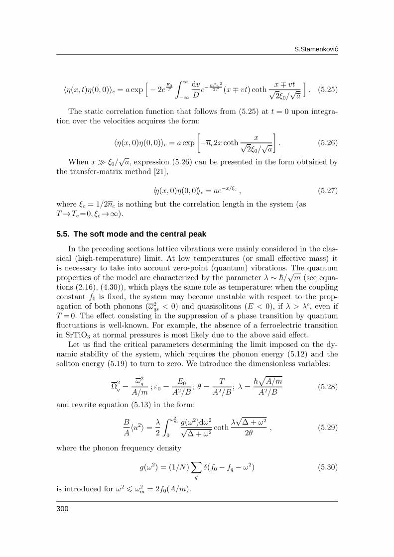
S.Stamenkovic

〈η(x, t)η(0, 0)〉c = a exp[

− 2eE0

T

∫ ∞

−∞

dv

De−

m∗v2

2T (x∓ vt) cothx∓ vt√2ξ0/

√a

]

. (5.25)

The static correlation function that follows from (5.25) at t = 0 upon integra-tion over the velocities acquires the form:

〈η(x, 0)η(0, 0)〉c = a exp

[

−nc2x cothx√

2ξ0/√a

]

. (5.26)

When x≫ ξ0/√a, expression (5.26) can be presented in the form obtained by

the transfer-matrix method [21],

〈η(x, 0)η(0, 0)〉c = ae−x/ξc , (5.27)

where ξc = 1/2nc is nothing but the correlation length in the system (asT→Tc=0, ξc→∞).

5.5. The soft mode and the central peak

In the preceding sections lattice vibrations were mainly considered in the clas-sical (high-temperature) limit. At low temperatures (or small effective mass) itis necessary to take into account zero-point (quantum) vibrations. The quantumproperties of the model are characterized by the parameter λ ∼ ~/

√m (see equa-

tions (2.16), (4.30)), which plays the same role as temperature: when the couplingconstant f0 is fixed, the system may become unstable with respect to the prop-agation of both phonons (ω2

qs < 0) and quasisolitons (E < 0), if λ > λc, even ifT =0. The effect consisting in the suppression of a phase transition by quantumfluctuations is well-known. For example, the absence of a ferroelectric transitionin SrTiO3 at normal pressures is most likely due to the above said effect.

Let us find the critical parameters determining the limit imposed on the dy-namic stability of the system, which requires the phonon energy (5.12) and thesoliton energy (5.19) to turn to zero. We introduce the dimensionless variables:

Ω2

q =ω2q

A/m; ε0 =

E0

A2/B; θ =

T

A2/B; λ =

~√

A/m

A2/B(5.28)

and rewrite equation (5.13) in the form:

B

A〈u2〉 = λ

2

∫ ω2m

0

g(ω2)dω2

√∆+ ω2

cothλ√∆+ ω2

2θ, (5.29)

where the phonon frequency density

g(ω2) = (1/N)∑

q

δ(f0 − fq − ω2) (5.30)

is introduced for ω2 6 ω2m = 2f0(A/m).

300

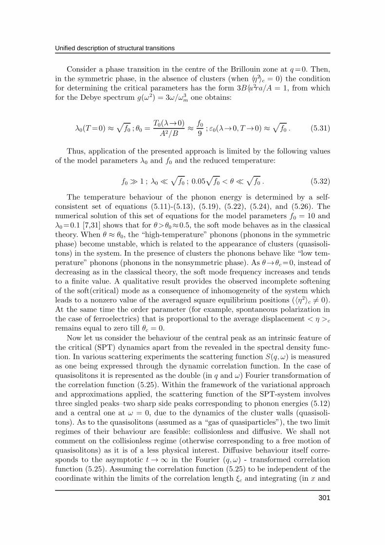
Unified description of structural transitions

Consider a phase transition in the centre of the Brillouin zone at q=0. Then,in the symmetric phase, in the absence of clusters (when 〈η2〉c = 0) the conditionfor determining the critical parameters has the form 3B〈u2ra/A = 1, from whichfor the Debye spectrum g(ω2) = 3ω/ω3

m one obtains:

λ0(T =0) ≈√

f0 ; θ0 =T0(λ→0)

A2/B≈ f0

9; ε0(λ→0, T→0) ≈

√

f0 . (5.31)

Thus, application of the presented approach is limited by the following valuesof the model parameters λ0 and f0 and the reduced temperature:

f0 ≫ 1 ; λ0 ≪√

f0 ; 0.05√

f0 < θ ≪√

f0 . (5.32)

The temperature behaviour of the phonon energy is determined by a self-consistent set of equations (5.11)-(5.13), (5.19), (5.22), (5.24), and (5.26). Thenumerical solution of this set of equations for the model parameters f0 = 10 andλ0=0.1 [7,31] shows that for θ>θ0≈0.5, the soft mode behaves as in the classicaltheory. When θ ≈ θ0, the “high-temperature” phonons (phonons in the symmetricphase) become unstable, which is related to the appearance of clusters (quasisoli-tons) in the system. In the presence of clusters the phonons behave like “low tem-perature” phonons (phonons in the nonsymmetric phase). As θ→θc=0, instead ofdecreasing as in the classical theory, the soft mode frequency increases and tendsto a finite value. A qualitative result provides the observed incomplete softeningof the soft(critical) mode as a consequence of inhomogeneity of the system whichleads to a nonzero value of the averaged square equilibrium positions (〈η2〉c 6= 0).At the same time the order parameter (for example, spontaneous polarization inthe case of ferroelectrics) that is proportional to the average displacement < η >c

remains equal to zero till θc = 0.

Now let us consider the behaviour of the central peak as an intrinsic feature ofthe critical (SPT) dynamics apart from the revealed in the spectral density func-tion. In various scattering experiments the scattering function S(q, ω) is measuredas one being expressed through the dynamic correlation function. In the case ofquasisolitons it is represented as the double (in q and ω) Fourier transformation ofthe correlation function (5.25). Within the framework of the variational approachand approximations applied, the scattering function of the SPT-system involvesthree singled peaks–two sharp side peaks corresponding to phonon energies (5.12)and a central one at ω = 0, due to the dynamics of the cluster walls (quasisoli-tons). As to the quasisolitons (assumed as a “gas of quasiparticles”), the two limitregimes of their behaviour are feasible: collisionless and diffusive. We shall notcomment on the collisionless regime (otherwise corresponding to a free motion ofquasisolitons) as it is of a less physical interest. Diffusive behaviour itself corre-sponds to the asymptotic t→ ∞ in the Fourier (q, ω) - transformed correlationfunction (5.25). Assuming the correlation function (5.25) to be independent of thecoordinate within the limits of the correlation length ξc and integrating (in x and

301

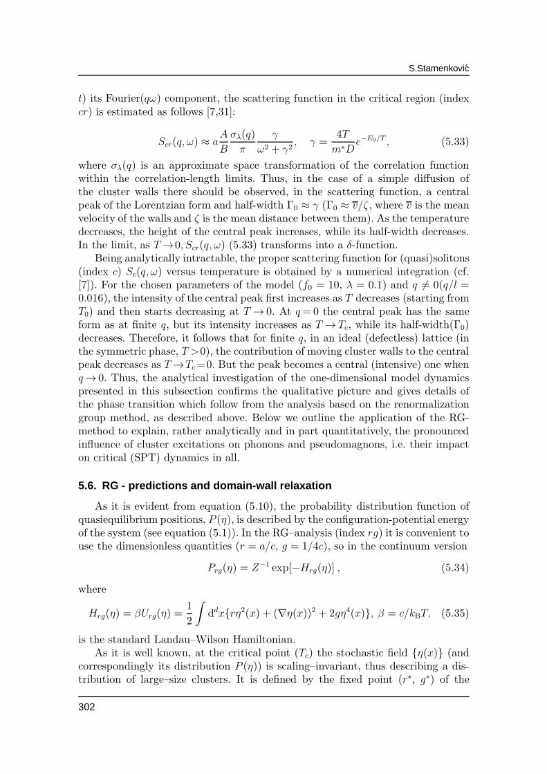
S.Stamenkovic

t) its Fourier(qω) component, the scattering function in the critical region (indexcr) is estimated as follows [7,31]:

Scr(q, ω) ≈ aA

B

σλ(q)

π

γ

ω2 + γ2, γ =

4T

m∗De−E0/T , (5.33)

where σλ(q) is an approximate space transformation of the correlation functionwithin the correlation-length limits. Thus, in the case of a simple diffusion ofthe cluster walls there should be observed, in the scattering function, a centralpeak of the Lorentzian form and half-width Γ0 ≈ γ (Γ0 ≈ v/ζ , where v is the meanvelocity of the walls and ζ is the mean distance between them). As the temperaturedecreases, the height of the central peak increases, while its half-width decreases.In the limit, as T→0, Scr(q, ω) (5.33) transforms into a δ-function.

Being analytically intractable, the proper scattering function for (quasi)solitons(index c) Sc(q, ω) versus temperature is obtained by a numerical integration (cf.[7]). For the chosen parameters of the model (f0 = 10, λ = 0.1) and q 6= 0(q/l =0.016), the intensity of the central peak first increases as T decreases (starting fromT0) and then starts decreasing at T → 0. At q=0 the central peak has the sameform as at finite q, but its intensity increases as T → Tc, while its half-width(Γ0)decreases. Therefore, it follows that for finite q, in an ideal (defectless) lattice (inthe symmetric phase, T >0), the contribution of moving cluster walls to the centralpeak decreases as T→Tc=0. But the peak becomes a central (intensive) one whenq→ 0. Thus, the analytical investigation of the one-dimensional model dynamicspresented in this subsection confirms the qualitative picture and gives details ofthe phase transition which follow from the analysis based on the renormalizationgroup method, as described above. Below we outline the application of the RG-method to explain, rather analytically and in part quantitatively, the pronouncedinfluence of cluster excitations on phonons and pseudomagnons, i.e. their impacton critical (SPT) dynamics in all.

5.6. RG - predictions and domain-wall relaxation

As it is evident from equation (5.10), the probability distribution function ofquasiequilibrium positions, P (η), is described by the configuration-potential energyof the system (see equation (5.1)). In the RG–analysis (index rg) it is convenient touse the dimensionless quantities (r = a/c, g = 1/4c), so in the continuum version

Prg(η) = Z−1 exp[−Hrg(η)] , (5.34)

where

Hrg(η) = βUrg(η) =1

2

∫

ddxrη2(x) + (∇η(x))2 + 2gη4(x), β = c/kBT, (5.35)

is the standard Landau–Wilson Hamiltonian.As it is well known, at the critical point (Tc) the stochastic field η(x) (and

correspondingly its distribution P (η)) is scaling–invariant, thus describing a dis-tribution of large–size clusters. It is defined by the fixed point (r∗, g∗) of the

302

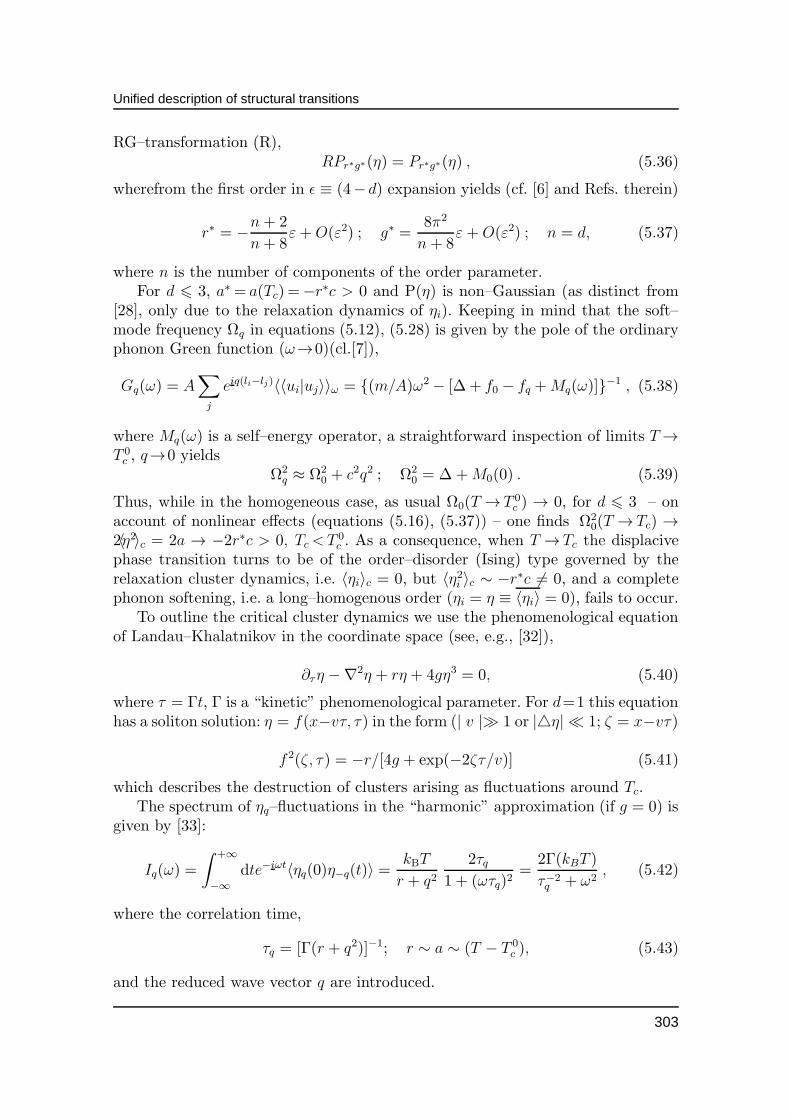
Unified description of structural transitions

RG–transformation (R),RPr∗g∗(η) = Pr∗g∗(η) , (5.36)

wherefrom the first order in ǫ ≡ (4− d) expansion yields (cf. [6] and Refs. therein)

r∗ = −n+ 2

n+ 8ε+ O(ε2) ; g∗ =

8π2

n+ 8ε+ O(ε2) ; n = d, (5.37)

where n is the number of components of the order parameter.For d 6 3, a∗ = a(Tc) =−r∗c > 0 and P(η) is non–Gaussian (as distinct from

[28], only due to the relaxation dynamics of ηi). Keeping in mind that the soft–mode frequency Ωq in equations (5.12), (5.28) is given by the pole of the ordinaryphonon Green function (ω→0)(cl.[7]),

Gq(ω) = A∑

j

eiq(li−lj)〈〈ui|uj〉〉ω = (m/A)ω2 − [∆ + f0 − fq +Mq(ω)]−1 , (5.38)

where Mq(ω) is a self–energy operator, a straightforward inspection of limits T→T 0c , q→0 yields

Ω2q ≈ Ω2

0 + c2q2 ; Ω20 = ∆+M0(0) . (5.39)

Thus, while in the homogeneous case, as usual Ω0(T → T 0c ) → 0, for d 6 3 – on

account of nonlinear effects (equations (5.16), (5.37)) – one finds Ω20(T → Tc) →

2〈η2〉c = 2a → −2r∗c > 0, Tc<T0c . As a consequence, when T → Tc the displacive

phase transition turns to be of the order–disorder (Ising) type governed by therelaxation cluster dynamics, i.e. 〈ηi〉c = 0, but 〈η2i 〉c ∼ −r∗c 6= 0, and a completephonon softening, i.e. a long–homogenous order (ηi = η ≡ 〈ηi〉 = 0), fails to occur.

To outline the critical cluster dynamics we use the phenomenological equationof Landau–Khalatnikov in the coordinate space (see, e.g., [32]),

∂τη −∇2η + rη + 4gη3 = 0, (5.40)

where τ = Γt, Γ is a “kinetic” phenomenological parameter. For d=1 this equationhas a soliton solution: η = f(x−vτ, τ) in the form (| v |≫ 1 or |η| ≪ 1; ζ = x−vτ)

f 2(ζ, τ) = −r/[4g + exp(−2ζτ/v)] (5.41)

which describes the destruction of clusters arising as fluctuations around Tc.The spectrum of ηq–fluctuations in the “harmonic” approximation (if g = 0) is

given by [33]:

Iq(ω) =

∫ +∞

−∞dte−iωt〈ηq(0)η−q(t)〉 =

kBT

r + q22τq

1 + (ωτq)2=

2Γ(kBT )

τ−2q + ω2

, (5.42)

where the correlation time,

τq = [Γ(r + q2)]−1; r ∼ a ∼ (T − T 0c ), (5.43)

and the reduced wave vector q are introduced.

303

S.Stamenkovic

By performing calculations for nonlinear effects (g 6= 0), using ansatz [32], theasymptotic spectral response (i.e. when q→ 0, ω ≪ 1, T → Tc) exhibits a centralpeak behaviour, thus reflecting a slow relaxation of cluster walls:

I(q=0, ω) ∼ kBTcπ

Γ

ω1+(2−η)/∆ω. (5.44)

The combination of the small correlation critical (η) and dynamical (∆ω) in-dices in equation (5.44) is given by the fixed point–parameter (g∗), i.e. by theε–expansion (cf. [6,32] and Refs. therein):

2− η

∆ω= 1− (g∗)2

8π49 ln(4/3) ≈ 1− ε2

2(n+ 8)ln(4/3) . (5.45)

To conclude, our theoretical findings based on the decomposing picture on“slow” and “fast” dynamical variables (equation (5.2)) show that (in accord withthe previous results, i.e. with various above mentioned approaches and suitableexperiments (cf. [7,11])) at some (“true”) critical temperature, Tc = T 0

c − δTc,δTc ∼ εT 0

c , the traditionally displacive system becomes structurally unstableagainst nonlinearly induced precursor clusters (i.e. by their order–disorder de-scribed by Ising–like variables ηi), so that 〈ηi(T→Tc)〉 → 0 without a completephonon softening: Ωq(q→0, T→Tc)→ 2〈η2i (Tc)〉 = 2a∗ ∼ ε. These clusters relax in apeculiar (dynamical) fashion: Iq(ω→0, q→0, T→Tc) ∼ ω−λ, λ . 2.

It should be gratifying that the present description can, at least in part, con-tribute to a better understanding of the SPT-dynamics, and to corroborate theappealing idea about the intrinsical “order–disorder origin” of universality.

5.7. The pseudospin dynamics: the limiting order–disorder transition anduniversal features of SPT

So far in the unified model description of SPT, i.e. in the corresponding self-consistent procedure exposed in the preceding sections, the dynamics of a pseu-dospin subsystem as described by the transverse Ising model (equation (4.6)) hasnot been taken into account unless intermediary through the average pseudospincomponents σx and σz(equation (4.21)) in the mean-field approximation. In thecase of the order-disorder SPT the soft-phonon picture of critical dynamics has tobe replaced by the concept of a tunnelling mode to a great extent resembling thephonon soft mode as the instability (critical) temperature is approached. Conse-quently, to be properly considered, the searching for the true, universal nature ofthe SPT, i.e. the real physical systems undergoing structural transitions, has totake into account, in an equal manner, all the intriguing features of critical dy-namics comprising phonons, tunnelling(magnon-like) and domain-wall excitations.Thus, it has surfaced an important conclusion that the system can be considered tohave not one, but three characteristic frequencies: the pseudoharmonic frequencywithin either side of a double well, the tunnelling frequency characterizing inter-well motion and a third one corresponding to domain-wall excitations (moving

304

Unified description of structural transitions

domain walls), by which the order parameter changes from one potential mini-mum to another inside the well defined distance [34,35]. Moreover, inside theseslow moving clusters the particles participate in a quantum-mechanical flippingsbetween their momentary rest positions ri(t) (equation (5.3)) which are describedby the pseudospin (i.e. transverse Ising) Hamiltonian (4.6).

Within the framework of a classical-quantum approach proposed recently [35],the pseudospin dynamics (as a counterpart of the displacive type dynamics) canbe treated in an almost analogous way. In the spirit of the preceding approach anddefinitions (section 4 and subsection 5.6), as well as introducing the representationof decomposed variables of the form (5.2), the pseudospin components can berepresented as follows:

Sαi = σα

i + χαi ; (5.46)

σxi = 〈Sζ

i 〉 sin θi cosϕi ;χxi = δSζ

i sin θi cosϕi + Sξi cos θi cosϕi − Sη

i sinϕi ,

σyi = 〈Sζ

i 〉 sin θi sinϕi ;χyi = δSζ

i sin θi sinϕi + Sξi cos θi sinϕi + Sη

i cosϕi ,

σzi = 〈Sζ

i 〉 cos θi ; χzi = δSζ

i cos θi − Sξi sin θi . (5.47)

Here ϕi, ψi = 0 and θi are the Euler angles after the unitary transformation in thepseudospin space Oxyz. Apparently, new temperature dependent axes 0ξηζ aresuch that the mean value 〈Si〉χα

i is directed along 0ζ-axis∗.

In the scheme of the local (site dependent) mean field approximation (LMFA)[35] angle θi is given by (see subsection 4.3)

sin θi = 2Ω/Hi, H2i = (2Ω)2 +H2

iz, H2iz ≃ (4J0σ

zi )

2, (5.48)

while angle ϕi is expressed via θi [36],

cosϕi =1

2λ sin θiβ2 + [(1− β2)(4λ2 sin2 θi − β2)]1/2 ;

λ =1

2sin θ0 , (5.49)

where sin θ0 corresponds to a monodomain at given temperature and β = v/c0 isthe velocity of the domain-wall (in units of its maximum value c0 = 2Ωl/~

√2, l-

the lattice constant) which evolves in the pseudospin space.The corresponding quasisoliton solution σz(x, t) is of the same form obtained

for η(x, t)(5.18) (by using the Lorentz transformation, x→y) as a consequence ofthe equilibrium condition i.e. minimization of the free energy of the pseudospinsubsystem for a given configuration σα

i :∗For simplicity we omitted the averaging index associated with magnon-like variables χα

i in

equation (5.47).

305

S.Stamenkovic

∂

∂σzi

F (σαi ) = 0 ;F (σα

i ) = −kBT ln Spχαi e

−βHIMTF (5.50)

where HIMTF is the pseudospin Hamiltonian (4.6).In the critical temperature region (T ∼ Tc), in the LMFA-approximation, the

above equation (5.50) acquires the same form (5.16) in which the following iden-tifications have to be carried out [35] (cf. also [11]):

η(x, t) ≡ 2σz(x, t) ; A ≡ 2[ βcΩ

sinh(βcΩ)

]2

kBTc , B ≡ J30

Ω2[1− βcJ0

cosh2(βcΩ)] ;

βc = 1/kBTc ; Tc ∼ J0 . (5.51)

By introducing the quantum (flipping) effects in the effective (average-crystal)lattice (the bar symbol being associated with such an approximation)-through theboson-like representation,

δSζi = −a+i a−i , S±

i =

√

2 〈Sζi〉 a∓i , (5.52)

or by directly using the adopted pseudospin Green function [7,19],

Gξξq (ω) = − H 〈Sζ〉

ω2 − ω2q

, (5.53)

the frequency of the pseudospin (tunnelling) mode is expressed in the well-knownbut slightly modified form [7,11,33-35];

ωq2 = H2(1− Jqsin

2 θ/J0) ; H2 = (2Ω)2 + (4J0)2〈(σz(x))2〉c . (5.54)

It is easily seen that the results analogous to the case of displacive SPT (elab-orated in the previous subsection) are obtained: with the onset of criticality anincomplete softening of the pseudospin (tunnelling) mode occurs,

ω2(q→0, T→Tc) ≃ (4J0)2〈(σz)2〉c 6= 0 , (5.55)

while in the spectral density of excitations a central peak of the form (5.44),

S(q = 0, ω) ∼ ω−λ, λ . 2, (5.56)

evolves as a consequence of the pseudospin domain-wall relaxation.Instead of extended conclusions usually presented at the end of each section,

it is gratifying that the present contribution can, at least in part, complete abetter understanding of the SPT dynamics and to corroborate, the more and moreappealing idea about the intrinsical order-disorder nature of SPT as its essentialuniversal feature. Although invalid in quantitative predictions, our unified model

306

Unified description of structural transitions

description of SPTs (bearing in mind simple approximations used) is illuminating,as Drs. Bruce and Cowley, great specialists in this field, stated in [11].

We hope that the theoretical results presented in this review have “displaced”and contributed to the “order” of some aspects of knowledge about the univer-sal nature of SPTs, as well as to a prompt further progress in all-inclusive SPTinvestigations.

Acknowledgement

I would like to gratify Prof. Academician I.R.Yukhnovskii for his kind invitationto participate in the special issue of the journal Condensed Matter Physics devotedto the 60th anniversary of Professor, Dr. Ihor Stasyuk, my dear colleague andan outstanding scientist. It was my great pleasure that I had an opportunity tocooperate with Dr. Ihor Stasyuk during all these years. I would like to express mywishes of all the best in his future scientific work and his life.

References

1. Stamenkovic S., Plakida N.M., Aksienov V.L., Siklos T., Phys. Rev B, 1976, vol 14,p. 5080; JINR, P17-9226, Dubna, 1975 (in Russian).

2. Stamenkovic S., Plakida N.M., Aksienov V.L., Siklos T., Ferroelectrics, 1976, vol 14,p. 655.

3. Stamenkovic S., Plakida N.M., Aksienov V.L., Siklos T., Acta Phys. Hung., 1977, vol 42,p. 265.

4. Stamenkovic S., Plakida N.M., Aksienov V.L., Siklos T., Acta Phys. Hung., 1977, vol 43,p. 99.

5. Stamenkovic S.,Plakida N.M., Aksienov V.L., Siklos T., Fizika, 1978, vol 10, Supple-ment 2, p. 122; Stamenkovic S., Plakida N.M., Aksienov V.L., Siklos T., Ferroelectrics,1980, vol 24, p. 255; JINR, P17-11856, Dubna, 1978 (in Russian);Aksenov V.L., D.Baatar, N.M. Plakida, S. Stamenkovic, JINR, P17-12961, Dubna, 1979 (in Russian).

6. Stamenkovic S., Plakida N.M, Aksienov V.L., Zagrebnov V.A., Fizika, 1980, vol 12,Supplement 1, p. 332; Aksenov V.L., Zagrebnov V.A., Plakida N.M., Stamenkovic S.,JINR, P17-80-576, Dubna, 1980 (in Russian).

7. Aksienov V.L., Plakida N.M., Stamenkovic S., Neutron scattering by Ferroelectrics,World Scientific, Singapore, 1989.

8. Plakida N.M, in Statistical Physics and Quantum Theory of Fields, 1973, ed. Bo-golyubov N.N., Nauka, Moscow, p. 205–240 (In Russian).

9. Fujiwara T., J. Phys. Soc. Japan, 1970, vol 29, p. 1282.10. Moore M.A., Williams H.C.W.L., J. Phys. C, 1972, vol 5, p. 3168.11. Bruce A.D, Cowley R.A. Structural Phase Transition, Taylor and Francis Ltd., Lon-

don, 1981.12. Vaks V.G., Larkin A.I., Zhurn. Eksp. Teor. Fiz., 1965, vol 49, p.975 (in Russian).13. Plakida N.M, Siklos T., Acta Phys. Hung., 1978, vol 45, p. 37.14. Aksienov V.L., Breter H., Kovalski Ya.M., Plakida N.M., Priezzhev V.B., Fiz.tverd.

tela, 1976, vol 18, p. 2920 (in Russian).

307

S.Stamenkovic

15. Gillis N.S. and Koehler T.R., Phys.Rev. Lett., 1972, vol 29, p. 369; Phys.Rev. B, 1973,vol 7, p. 4980; Phys.Rev., 1974, vol 9, p. 3806; Gillis N.S., Phys. Rev. B, 1975, vol 11,p. 309; Gillis N.S., Dynamical Properties of Solids, vol 2, ed. G.K. Horton and A.A.Maradudin, North–Holland, Amsterdam, 1975, p. 107.

16. Eisenriegler E., Phys.Rev. B, 1974, vol 9, p. 1029.17. Sokolov A.I., Fiz.Tverd. Tela, 1974, vol 16, p. 733 (in Russian).18. Elliot R.G., Krumhansl J.A., Leath P.L., Rev. Mod. Phys., 1974, vol 46, p.5080.19. Aksenov V.L., Schreiber J., Phys. Lett., 1978, vol 69A, p.56.20. Stasyuk I.V., Preprint ITF - 75-108P, 1975, Kiev (in Russian).21. Krumhansl J.A., Schrieffer J.R., Phys.Rev. B, 1975, vol 11, p.3535.22. Koehler T.R., Bishop A.R., Krumhansl J.A., Schrieffer J.R., Solid State Commun.,

1975, vol 17, p.1515; Schneider T., Stoll E., Phys.Rev. Lett. 1976, vol 36, p.1501;Phys.Rev.B, 1976, vol 13, p.1216; Phys.Rev. B, 1978, vol 17, p.1302.

23. Beck H., J. Phys.C, 1976, vol 9, p.33.24. Bruce A.D., Muller K.A., Berlinger W., Phys.Rev.Lett., 1979, vol 42, p.185.25. Reiter G.F., Berlinger W., Muller K.A., Phys.Rev. B, 1980, vol 21, p.1.26. Muller K.A., Lecture Notes in Physics, ed. Enz C.P., Springer-Verlag, Berlin, 1979,

p. 210.27. Bruce A.D., Schneider T., Phys.Rev. B, 1977, vol 16, p. 3991.28. Bruce A.D., Schneider T., Stoll E., Phys. Rev. Lett., 1979, vol 43, p. 1284.29. Beale P.D., Sarker S., Krumhansl J.A., Phys.Rev. B, 1981, vol 24, p. 266.30. Bishop A.R., Domany E., Krumhansl J.A., Phys.Rev., 1976, vol 14, p. 2966.31. Aksenov V.L., Didyk A.Yu., Yushankhaj V.Yu, Solid State Commun., 1981, vol 40,

p. 825; Fiz. Niz. Temp., 1982, vol. 8, p. 626 (in Russian).32. Patashinskii A.Z., Pokrovskii V.L., Fluctuation Theory of Phase Transitions, Nauka,

Moscow, 1975, vol. 5, p.211 (in Russian); ibid, II edition, Nauka, Moscow 1982, p. 277(in Russian).

33. Blinc R, Zeks B., Soft Modes in Ferroelectrics and Antiferroelectrics, North-Holland,Amsterdam 1974, p. 54.

34. Lines M.E. and Glass A.M., Principles and Applications of Ferroelectrics and RelatedMaterials, Clarendon Press, Oxford, 1977, Sections 1 and 2.

35. Stamenkovic S., Simp. Fiz. Kondenz. Materije, ed. M. Davidovic, Kladovo, 1997, p. 129(in Serbian).

36. Prelovsek P., Sega I., J. Phys. C: Solid State Phys. 1981, vol. 14, 3231.

308

Unified description of structural transitions

Уніфікований модельний опис структурних фазових

переходів типу порядок-безпорядок та типу

зміщення

С.Стаменкович

Інститут ядерних наук, Лабораторія теоретичної фізики та фізики

конденсованої речовини, Бєлград, Пошт. Скр. 522, Югославія

Отримано 7 липня 1998 р.

Зроблено огляд і часткове оновлення серії робіт автора з співавтора-

ми [1-7], присвяченої уніфікованому модельному опису структурних

фазових переходів (СФП) у сегнетоелектриках та споріднених ма-

теріалах.

Виходячи з загального гамільтоніану попарно зв’язаних ангармоніч-

них (четвірних) осциляторів та враховуючи концепцію локальних нор-

мальних координат, запропоновано уніфікований модельний опис

систем з СФП обидвох типів: порядок-безпорядок і зміщення.

В рамках стандартної варіаційної процедури формулюється гібри-

дизований псевдоспін-фононний гамільтоніан введенням змінних,

що відповідають фононним, магноно-подібним (з переворотом) і не-

лінійним (типу доменної стінки) зміщенням атомів, що беруть участь

у СФП. Це досягається представленням колективного руху атомів че-

рез декілька квазірівноважних положень (в найпростішому випадку

- двох) як повільного тунельного зміщення (розбитого на магноно-

подібні і солітоно-подібні відхилення) додатково до порівняно швид-

ких фононних осциляцій навколо неоднорідних миттєвих положень

спокою, в свою чергу індукованих збудженнями типу доменної стінки

(солітонами).

Якісний і кількісний аналізи показали, що СФП (першого чи дру-

гого роду) можуть бути типу зміщення (керованих м’якою фонон-

ною модою), порядок-безпорядок (керованих тунельною магноно-

подібною м’якою модою) чи змішаного типу залежно як від енергії

зв’язку між атомами, так і від їхньої нульової точки коливної енергії. В

області критичної температури збудження типу доменної стінки при-

водять до утворення мікродоменів (кластерів впорядкованої фази),

які індукують СФП класу універсальності Ізінгівського типу. Має міс-

це неповне пом’якшення фононної чи псевдомагнонної моди і у спек-

тральній густині збуджень виникає центральний пік, викликаний по-

вільною релаксацією кластерів.

Ключові слова: структурні фазові переходи, порядок-безпорядок,

перехід зміщення

PACS: 63.70.+h, 77.80.Bh, 64.60.-i, 64.60.Cn

309

310