This article was downloaded by: [UZH Hauptbibliothek / Zentralbibliothek Zürich]On: 11 July 2014, At: 23:35Publisher: Taylor & FrancisInforma Ltd Registered in England and Wales Registered Number: 1072954 Registered office: MortimerHouse, 37-41 Mortimer Street, London W1T 3JH, UK

Communications in Statistics - Theory and MethodsPublication details, including instructions for authors and subscription information:http://www.tandfonline.com/loi/lsta20

The two-sample t test versus satterthwaite'sapproximate f testBarry K. Moser a , Gary R. Stevens a & Christian L. Watts aa Department of Statistics , Oklahoma State University , Stillwater, OK, 74078Published online: 27 Jun 2007.

To cite this article: Barry K. Moser , Gary R. Stevens & Christian L. Watts (1989) The two-sample t test versussatterthwaite's approximate f test, Communications in Statistics - Theory and Methods, 18:11, 3963-3975, DOI:10.1080/03610928908830135

To link to this article: http://dx.doi.org/10.1080/03610928908830135

PLEASE SCROLL DOWN FOR ARTICLE

Taylor & Francis makes every effort to ensure the accuracy of all the information (the “Content”) containedin the publications on our platform. However, Taylor & Francis, our agents, and our licensors make norepresentations or warranties whatsoever as to the accuracy, completeness, or suitability for any purposeof the Content. Any opinions and views expressed in this publication are the opinions and views of theauthors, and are not the views of or endorsed by Taylor & Francis. The accuracy of the Content shouldnot be relied upon and should be independently verified with primary sources of information. Taylorand Francis shall not be liable for any losses, actions, claims, proceedings, demands, costs, expenses,damages, and other liabilities whatsoever or howsoever caused arising directly or indirectly in connectionwith, in relation to or arising out of the use of the Content.

This article may be used for research, teaching, and private study purposes. Any substantial or systematicreproduction, redistribution, reselling, loan, sub-licensing, systematic supply, or distribution in anyform to anyone is expressly forbidden. Terms & Conditions of access and use can be found at http://www.tandfonline.com/page/terms-and-conditions

COMMUN. STATIST.-THEORY METH., 18(11), 3963-3975 (1989)

THE TWO-SAMPLE T TEST VERSUS SATTERTHWAITE'S APPROXIMATE F TEST

Barry K. Moser Gary R. Stevens

Christian L. Watts

Department of Statistics Oklahoma State University

Stillwater, OK 74078

K e y Words and Phrases: Size; power; preliminary variance test.

ABSTRACT

A comparison between the two-sample t test and Satterthwaite's ap- proximate F test is made, assuming the choice between these two tests is based on a preliminary test on the variances. Exact formulas for the sizes and powers of the tests are derived. Sizes and powers are then calculated and compared for several situations.

1. INTRODUCTION

The problem of testing the equality of the means from two independent normally distributed populations is covered in every elementary statistics text book. Under the assumption that the variances of the two populations are equal, the t test is recommended. If the variances of the two popu- lations are unequal, then an alternative procedure, such as Satterthwaite's Approximate F test (1946), is suggested. From a practitioner's standpoint, this approach to the problem is unsatisfactory. Generally, in problems where the means are unknown, so are the variances. To overcome the difficulty of choosing between the t test and Satterthwaite's test, many authors recom- mend a formal preliminary test of a: = a:. If 0: = a: is not rejected in this preliminary test then the t test on the means is performed; otherwise Satterthwaite's test on the means is performed.

3963

Copyright O 1989 by Marcel Dekker, Inc.

Dow

nloa

ded

by [

UZ

H H

aupt

bibl

ioth

ek /

Zen

tral

bibl

ioth

ek Z

üric

h] a

t 23:

35 1

1 Ju

ly 2

014

3964 MOSER, STEVENS, AND WATTS

Although the preliminary variance test seems to resolve the difficulty of deciding between the t test and Sattert,hwaite's test, some important ques- tions remain unanswered. First, how are the size and power of the test on the means affected by the preliminary variance test? Second, what significance level is most appropriate f ~ r the pre!irnisarg test on the variances?

To address these questions, some notation is required. Let XI , . . . , x,, and yl , . . . , y,, be independent random samples from two normally dis- tributed populations where x ; - N ( p l , a:) and yj - N(p2,ai) for i = 1,. . . , n l and j = 1,. . . ,nz.

The usual test for Ho : u: = a: versus HI : a; # a; is to calculate

1-s! and reject Ho if F' > F ~ : - ~ or F' < Fnz<,nl-l where o is the pre- scribed variance test significance level, F:', is the 10Q(? - a*) percentile

- 3 -

point of an F distribution with a and b degrees of freedom, a! = Inl - I)-' ~~~1 ( x i - 3)" 3: = (n2 - I)-' ~ ~ ~ l ( y j - $j)2, 6 = xy$ x;/nl and

3 = Cyzl y j / n ~ . If Ho is not rejected, then the test for H l ; p1 = p2 versus H; : p1 # pa - .

(or H," : pl = p2 versus H i : pl > p z ) is to calculate

and reject H l if t m 2 > Ff,nl+n2-2 (or reject If; if t* > t6,nl+nr-2) where 5 is the prescribed means test significance level and si = i(n1 - 1)s: i- (nz - l)s:]/(nl + na - 2). Test procedure (2) is equivalent to the usual two sample t test for H,*.

If Ho is rejected, then the Satterthwaite criterion for testing H,* versus H; (or H; versus Hz*) is to calculate

and reject H,* if t**' > F!,, (or reject B$ if t** > ta,,), for the same pre- scribed significance level 6 given in (2) with

Dow

nloa

ded

by [

UZ

H H

aupt

bibl

ioth

ek /

Zen

tral

bibl

ioth

ek Z

üric

h] a

t 23:

35 1

1 Ju

ly 2

014

T TEST VERSUS F TEST 3965

It should be noted that if the re scribed variance test significance level, a, is set to 0 then Ho is accepted and the t test (2) for H,' is always per- formed. Likewise, if a is set to 1 then the Satterthwaite test (3) for H,' is always performed. Therefore, specifying an a level of 0 (or 1) is equiva- lent to performing a t test (or Satterthwaite test) without any preliminary test for Ho. For purposes of identification, the preliminary test for Ho with 0 < a < 1 followed by a t test or Satterthwaite test for H,' will be referred to as the Sometimes Satterthwaite test (SS test). Performing a t test for H: without any preliminary test for Ho (i.e. a = 0), will be referred to as an Always t test (AT test). Using a Satterthwaite test for H: without any preliminary test for Ho (i.e. a = I), will be referred to as an Always Satterthwaite test (AS test).

Previous work has been done on the problem of preliminary tests of significance. Most notable is a paper by Bozovich, Bancroft and Hartley (195G), who investigated the problem of pooling in analysis of variance ap- plications. Gurland and McCullough (1962) examined the effects of a pre- liminary variance test on the power of an equality of means test developed by McCullough, Gurland and Rosenberg (1960). However, none of these papers addressed the Satterthwaite test. Others have investigated the Satterthwaite test in detail, Studies in this area include works by Cochran (1951)) Hudson and Krutchkoff (1968)) Davenport and Webster (1973), Lorenzen (1987) and Best and Raynor (1987). These authors investigated the AS test but did not address the problems associated with a preliminary test for Ho.

The authors believe that this paper extends the present literature by ex- amining the t test and Satterthwaite's test in conjunction with a preliminary variance test. The discussion in this paper is divided into four parts:

a) exact formulas for size and power calculations are given in Section 2, b) evaluations of the size for various values of 5, a, n1, n2 and 6 = ui/u;

are presented in Section 3, c) evaluations of the power for various values of 6, a, n l , nz, 8 and X =

(p2 - p1)~/[2(012/n1 + u;/n2)] are given in Section 4 and d) recommendations and conclusions are provided in Section 5.

2. EXACT FORMULAS FOR THE SIZE AND POWER CALCULATIONS

The formulas for the size and power calculations of the SS test are presented below. It will be shown that these formulas can be adapted to also calculate the sizes and powers of the AT test and AS test.

The prclbability of rejecting H,* : ,ul = p2 for the SS test is a function of n l , na, 8, 6 , CY and A. When X = 0, the probability of rejecting H,' is the size of the SS test. The power of the SS test corresponds to the probability

of rejecting H; for any X > 0. In either case, the rob ability of rejecting H,' is expressed as the sum of two mutually exclusive alternatives:

Dow

nloa

ded

by [

UZ

H H

aupt

bibl

ioth

ek /

Zen

tral

bibl

ioth

ek Z

üric

h] a

t 23:

35 1

1 Ju

ly 2

014

3966 MOSER, STEVENS, AND WATTS

P(reject H$) = P(reject H t and do not reject H o )

+P(reject H; and reject Ho) (5)

For the two sided alternative H; : p1 # p2, equation (5) can be restated as 1-E

5 reject H;) = ~ ( t * ~ > F : , ~ ~ + ~ ~ - ~ and Fn2Gln1-l < u < ~ l ~ - ~ , ~ ~ - l )

+P(t**2 > F:, and u < F:L-!,~~-~)

+p(t**' > Ff,. and u > F ~ : - ~ ,,i-,) (6)

where u = si/s:. Using Cochran (1951), the first term on the right hand side of (6) can be rewritten as

and

This reformulation of the first term on the right hand side of (6) is accom- plished by multiplying tm2 and Ff,n1+n3-2 by the denominator of t*2 and dividing each result by the denominator of Q*.

The statistic Q* is distributed as an F random variable with 1 and nl + nz - 2 degrees of freedom and noncentrality parameter A. The variable u/e is distributed as a central F random variable with n2 - 1 and nl - 1 degrees of freedom. The statistic Q* is independent of u since the ratio of two independent chi-square random variables is independent of their sum. So, Qm and g(u) are also independent. Therefore, the probability value given in (7) can be expressed as

where f (u), the density function of u, is

for u > 0 and f (u) = 0 otherwise. The second term on the right hand side of (6) can similarly be rewritten

as:

Dow

nloa

ded

by [

UZ

H H

aupt

bibl

ioth

ek /

Zen

tral

bibl

ioth

ek Z

üric

h] a

t 23:

35 1

1 Ju

ly 2

014

T TEST VERSUS F TEST 3967

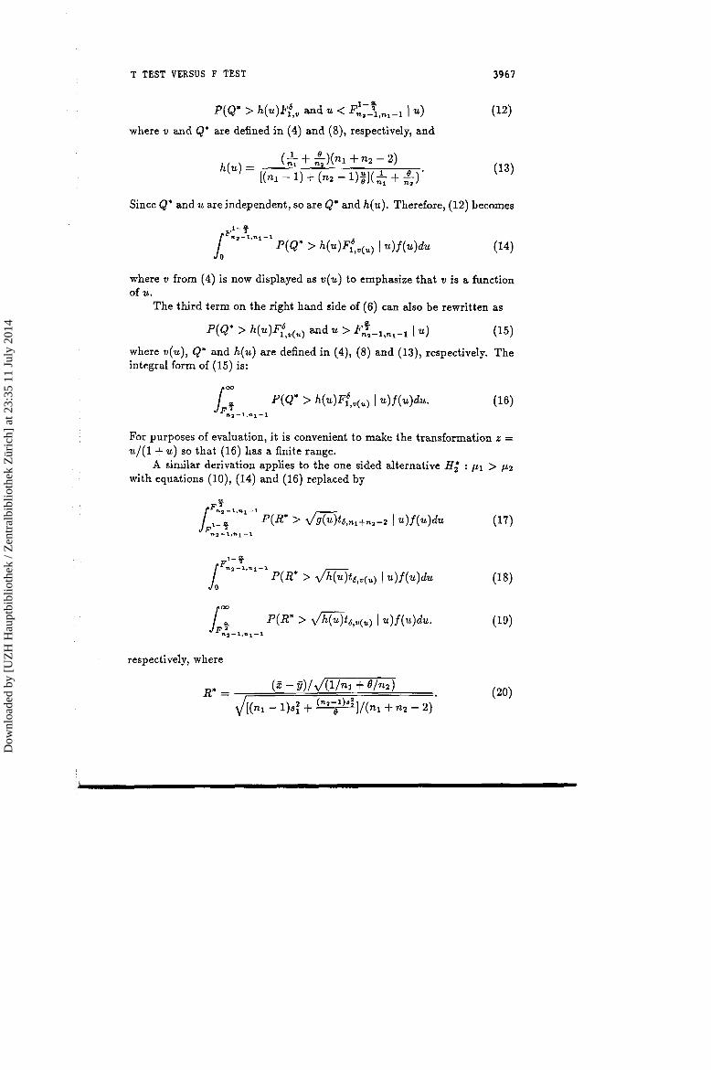
1-5 P(Q* > h(u)Ff,v and u < Fn2-l,nl-1 I u ) (12)

where v and Q* are defined in (4) and (8), respectively, and

Since Q* and u are independent, so are Q* and h(u). Therefore, (12) becomes

where v from (4) is now displayed as v(u) to emphasize that v is a function of u.

The third term on the right hand side of ( 6 ) can also be rewritten as

' ( Q * > h ( ~ ) k ; q ~ ( ~ ) and u > ~n!-l,n~-, I U ) (15)

where ~ ( u ) , Q* and h(u) are defined in (4) , (8) and (13), respectively. The integral form of (15) is:

For purposes of evaluation, it is convenient to make the transformation z = u / (1 + u ) SO that (16) has a finite range.

A similar derivation applies to the one sided alternative Hi : p1 > p2 with equations ( l o ) , (14) and (16) replaced by

respectively, where

Dow

nloa

ded

by [

UZ

H H

aupt

bibl

ioth

ek /

Zen

tral

bibl

ioth

ek Z

üric

h] a

t 23:

35 1

1 Ju

ly 2

014

3968 MOSER, STEVENS, AND WATTS

The statistic R* is distributed as a t random variable with ni +n2 -2 degrees of freedom and noncentrality parameter A.

The size and power of the SS test on H: versus H; (or H,' versus Hi) are calculated by numerically integrating (lo), (14) and (16) (or (17), (18) and (19)) and summing the three values with 0 < a < 1. The size and power of the AT test for H,* versus H; (or H,* versus Hz*) can be calculated from (10) (or from (17)) with the limits of integration set at 0 and oo. The size and power of the AS test are calculated from (16) (or from (19)) with the limits set at 0 to m. For purposes of evaluation, the infinite limits are again changed to a finite range by transforming u to z = u/ ( l + u).

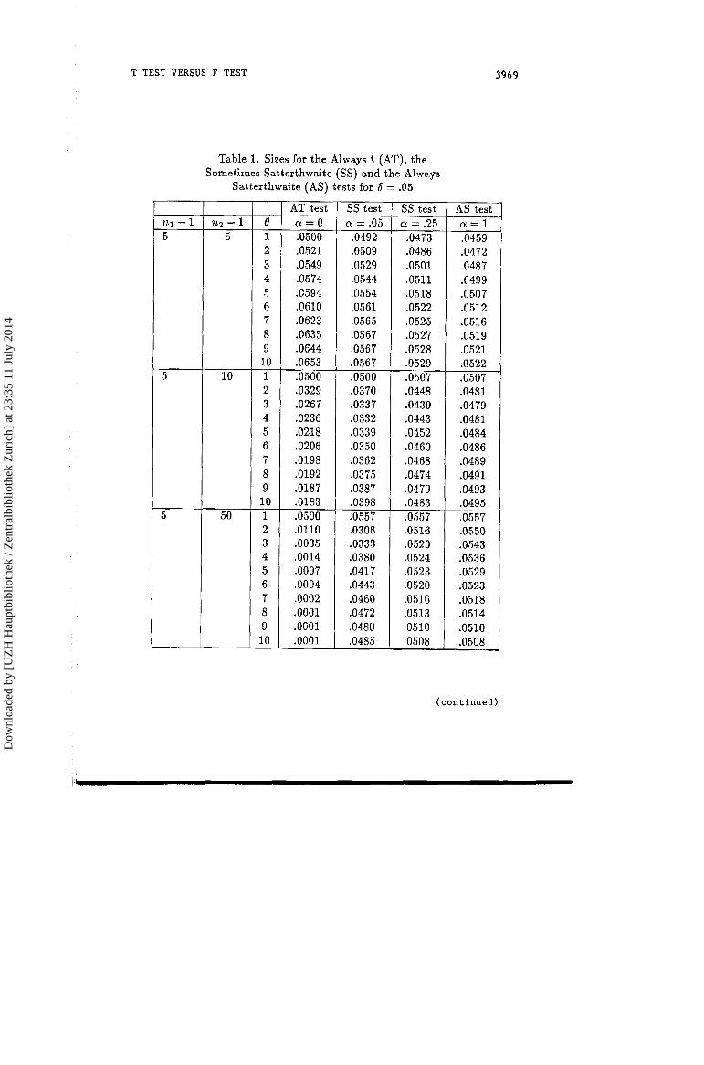
3. DISCUSSION OF THE SIZE CURVES

The sizes of the SS test, the AT test and the AS test are functions of n l , 722, 0, S and a. The sizes of the SS, AT and AS tests are not always equal to 6, but vary about this prescribed significance level as n l , nl, 0 and a vary. Sizes were calculated for nl - 1 = 5,10,20,50; nz - 1 = 5,10,20,50; 9 = 1,2,. . . ,10 and a = 0, .05, .lo, .25,1 (where a = 0 is the AT test, a = .05, . lo, .25 are three different levels for the SS test and a = 1 is the AS test). Values of 6' < 1 were not run to avoid redundance since combinations of nl , n2, 0 are equivalent to combinations of nz, ni , 110. The results for 6 = .01 and .05 display the same patt,ern of differences, so the 6 = .05 results are presented for illustrative purposes. Size calculations were performed for both alternatives H; and H;. Results for these two alternatives again display the same pattern of differences, so the two sided alternative Hi results are presented.

Test sizes are provided in Table 1 for various combinations of 8, nl - 1, nz - 1 and a. The table does not include all of the sizes calculated, but it does provide a representative illustration.

From Table 1, it is clear that if nl = nz then the AT, AS and SS tests all have sizes that are very close to S = -05 for all values of 0. If nl > na (i.e. the sample with the smaller variance has the larger sample size) then the SS test displays marked peaks and the size of the AT test monotonically increases away from S = .05 as 9 increases. If nl < nz (i.e. the sample with the smaller variance has the smaller sample size) then the SS test displays marked depressions and the size of the AT test monotonically decreases away from S = .05 as 0 increases.

For fixed values of nl # n2 and 9, the amount of the size disturbance increases as a decreases, with the largest disturbances occurring for a = 0, the AT test, and the smallest disturbances occurring for a = 1, the AS test. Finally, for fixed values of a and 9, the size disturbances increase as the sample sizes become more and more unequal.

The conclusions on size control are now summarized. If the two sample sizes are equal, nl = n2, then the AT test, the AS test and the SS test provide very stable sizes close to the prescribed significance level, 6. If nl # nz, then the AS test controls the size close to the prescribed significance level, 6.

Dow

nloa

ded

by [

UZ

H H

aupt

bibl

ioth

ek /

Zen

tral

bibl

ioth

ek Z

üric

h] a

t 23:

35 1

1 Ju

ly 2

014

T TEST VERSUS F TEST

Table 1. Sizes for the Always t (AT), the Sometimes Satterthwaite (SS) and the Always

Satterthwaite (AS) tests for 6 = .05 -- AT test a = 0 .0500 .OX21 .a549 .0574 .0594 .0610 ,0623 .0635 .0644 .0653 .0500 ,0329 .0267 .0236 .0218 .0206 .0198 .0192 A187 .0183 .0500 .0110 .0035 .0014 .0007 .0004 .0002 .0001 .0001 .0001

SS test a = .05

,0492 .0509 .0529 .0544 .0554 .0561 .0565 .0567 .0567 .0567 .0500 .0370 .0337 .0332 .0339 .0350 .0362 .0375 .0387 .0398 .0657 .0308 .0333 .0380 .0417 .OM3 .0460 .0472 .0480 .0485

SS test a = .25

.0473

.0486

.0501

.0511

.0518

.OFi22

.0525

.0527

.0628

.0529

.0507

.0448

.0439

.0443

.0452

.a460

.0468

.0474

.0479

.0483

.0557

.0516

.0520

.0524

.0523

.0520

.0516

.0513

.0510 ,0508

AS test a = l .(-I459 .0472 .0487 A499 .0507 .0512 .0516 .0519 .0521 .0522 .0507 .0481 .0479 .048l .0484 .0486 .0489 .0491 .0493 .0495 .CIS57 .0550 .0543 .OK36 .0529 .0523 .OR18 .OS14 .0510 .0508

(con t i m e d )

Dow

nloa

ded

by [

UZ

H H

aupt

bibl

ioth

ek /

Zen

tral

bibl

ioth

ek Z

üric

h] a

t 23:

35 1

1 Ju

ly 2

014

MOSER, STEVENS, AND WATTS

Table 1. (continued)

AT test a=O .0500 .0763 ,0945 .lo76 .I174 .I251 .I312 .I362 .I403 .I439 .0500 .0513 ,0529 .0543 .0554 .0562 .0570 .0576 .0581 .0585 .0500 .0154 .0069 .0038 .0024 .0017 .0012 .0010 .0008 .0007

SS test SS test a = .25

,0507 .0607 .0630 .0626 .0615 .0601 .0589 .0579 .0570 .0563 ,0488 .0496 .0501 .0503 ,0505 .0506 .0507 .0507 .0507 .0507 .0513 .0476 .0492 .0499 .0499 .0499 .0499 .0498 .0498 .0498

AS test

Dow

nloa

ded

by [

UZ

H H

aupt

bibl

ioth

ek /

Zen

tral

bibl

ioth

ek Z

üric

h] a

t 23:

35 1

1 Ju

ly 2

014

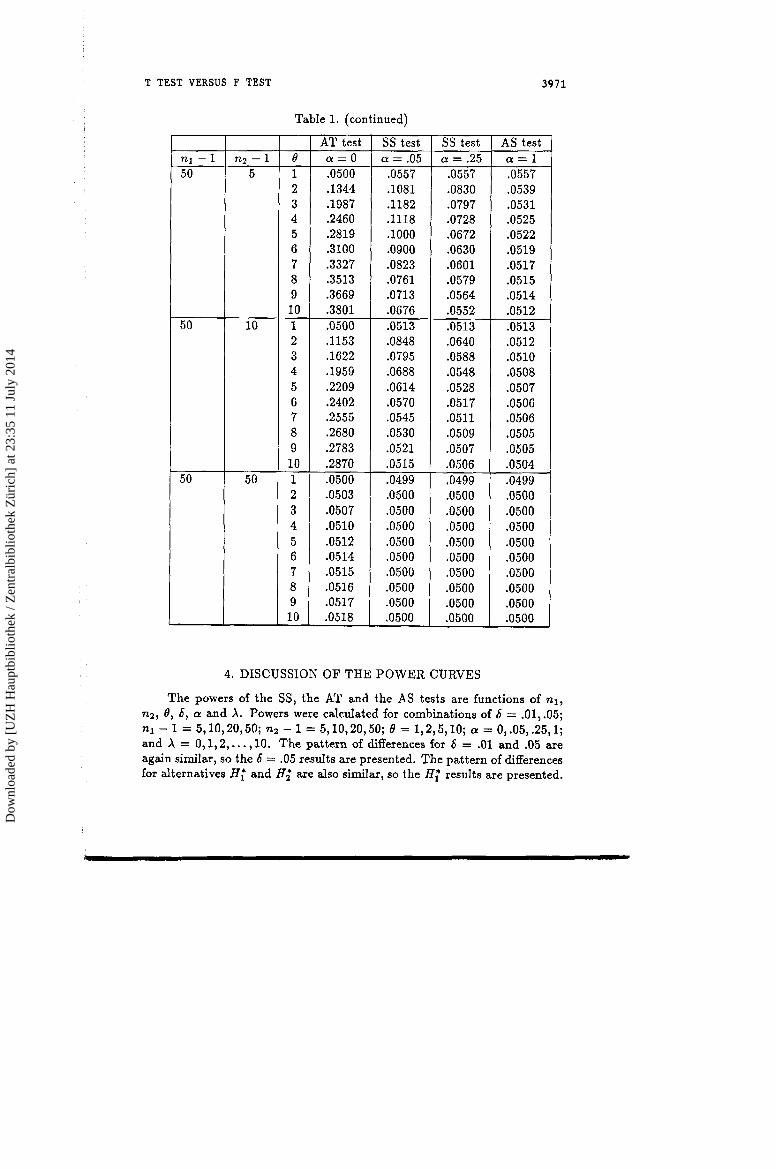
T TEST VERSUS F TEST

Table 1. (continued)

AT test a=O ,0500 .I344 .I987 .2460 .2819 .3100 .3327 .3513 .3669 .3801 .0500 .I153 .I622 .I959 .2209 .2402 .2555 .2680 .2783 .2870 ,0500 .0503 .0507 .0510 .0512 .0514 .0515 ,0516 .0517 .0518

SS test a = .05 .0557 .I081 .I182 .I118 .I000 .0900 .0823 .0761 .0713 .0676 .0513 .0848 .0795 .0688 .0614 .0570 .0545 .0530 .0521 .0515 .0499 -0500 .0500 .0500 ,0500 ,0500 .0500 ,0500 .0500 .0500

SS test a = .25

.a557

.0830

.0797

.0728

.0672

.0630

.Of301

.0579

.0564

.0552

.0513

.0640

.0588 ,0548 ,0528 .0517 .0511 ,0509 .0507 .0506 ,0499 .0500 .0500 .0500 .0500 .0500 .0500 .0500 .0500 .0500

AS test a = 1 ,0557 .0539 .0531 .0525 .0522 .0519 .0517 .0515 .0514 .0512 .0513 .0512 .0510 .0508 .0507 .0506 .0506 .0505 .0505 .0504 .0499 .0500 .0500 .0500 .0500 .0500 .0500 .0500 .0500 .0500

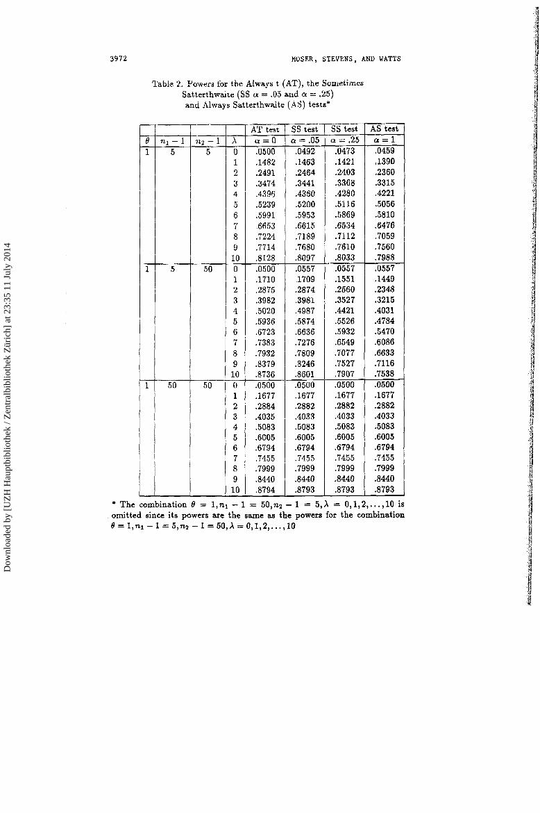
4. DISCUSSION OF THE POWER CURVES

The powers of the SS, the AT and the AS tests are functions of n l , n2, 8, 6, a and A. Powers were calculated for combinations of 6 = .01, .05; n l - 1 = 5,10,20,50; n l - 1 = 5,10,20,50; 8 = 1,2,5,10; a = 0, .05, .25,1; and X = 0,1,2 ,... , l o . The pattern of differences for 5 = .O1 and .05 are again similar, so the 6 = .05 results are presented. The pattern of differences for alternatives Hf and Hz* are also similar, so the H: results are presented.

Dow

nloa

ded

by [

UZ

H H

aupt

bibl

ioth

ek /

Zen

tral

bibl

ioth

ek Z

üric

h] a

t 23:

35 1

1 Ju

ly 2

014

3972 MUSER, STEVENS, AND WATTS

Table 2. Powers for the Always t (AT), the Sometimes Satterthwate (SS u = .05 and a = 3.5) and Always Satterthwaite (AS) tests'

..- AT test a = o .0500 ,1482 2491 ,3474 .43% .5239 .5991 6653 .7224 .7714 .8128 .0500 .I710 287.5 .3982 5020 .5936 .6723 .7383 .7932 .8373 ,8736 .0500 .I677 ,2884 .4035 -5083 .6005 A794 .7455 .7999 .8440 3794

---...- SS test -- a = .05 .0492 .I463 .2464 .3441 .4350 .5200 .5953 .6615 .7189 .7680 .8097 .0557 1709

.2874

.3981

.4987

.58'54

.6636

.7276

.7809

.8246

.8601

.0500

.I677

.2882 A033 .5083 ,6005 .6794 .7455 .7999 .8440 .8793

SS test -- a = -25 .0473 .I421 .2403 .3368 ,4280 .5116 .5869 ,6534 .7P12 .7610 A033 .0557 .I551 .2560 .3527 .4421 .5526 .5932 .6549 .TO77 .7527 .7907 .0500 .I677 ,2882 .4033 .5083 .6005 .6794 .7455 .7999 .8440 .8793

--- AS test -- a = l ,0459 .I390 .2360 ,3315 .4221 .5056 .5810 .6476 ,7059 .7560 .7988 .0557 .I449 ,2348 ,3215 .4031 .4784 .5470 .6086 .6633 .7116 .7538 .0500 .I677 .2882 .4033 .5083 .6005 .6794 .7455 .7999 .8440 .8793

The combination 6 = 1, nl - 1 = 50,n2 - 1 = 5, X = 0,1,2,. . . ,10 is omitted since its powers are the same as the powers for the combination B = l , n 1 - 1 = 5 , n ~ - l = 5 0 , X = 0 , 1 , 2 ,..., 10

Dow

nloa

ded

by [

UZ

H H

aupt

bibl

ioth

ek /

Zen

tral

bibl

ioth

ek Z

üric

h] a

t 23:

35 1

1 Ju

ly 2

014

Table 2. (continued)

SS test a = .05 .0567 .I476 .2379 .3238 .4062 .4811 .5490 .6101 .6642 ,7120 ,7538 .0485 .I493 .2500 .3453 .4320 .5088 .5755 .6328 .6817 .7231 .7583 .0676 .I475 .2276 .3058 .3806 .4509 .5160 .5757 .6297 .6781 .7214 .0500 .I662 .2853 ,3993 .5033 .5950 .6737 .7400 .7948 ,8394 3751

SS test a = .25

.0529

.I404 ,2287 .3144 .3955 .4706 .5391 ,6009 .6560 .7047 .7475 .0508 .I600 .2714 .3783 .4766 .5643 .6410 .7066 ,7620 .8081 .8462 A552 ,1359 .2176 .2975 .3704 .4458 .5122 .5728 .6276 .6766 .7202 .0500 .I622 .2853 3993 .5033 .5949 .6737 .7399 ,7947 .8393 3751

AS test a = l .0522 .1395 .2277 .3134 .3945 .4697 .5384 .6003 .6555 .7043 .7471 .0508 .1601 .2717 .3788 .4774 .5653 .6421 .7080 .7636 .8099 ,8481 .0512 ,1324 ,2149 .2955 ,3724 .4446 .5113 .5722 .6272 .6763 .7200 .0500 .1662 .2853 .3993 .5033 .5949 .6737 .7399 ,7947 .8393 .8751 -

Dow

nloa

ded

by [

UZ

H H

aupt

bibl

ioth

ek /

Zen

tral

bibl

ioth

ek Z

üric

h] a

t 23:

35 1

1 Ju

ly 2

014

3974 MOSER, STEVENS, AND WATTS

Power values are provided in Table 2 for various combinations of A, a, 8, nl - 1 and n2 - 1. Again, Table 2 does not depict all of the combinations run, but does portray a representative illustration.

From Table 2, if nl = n2 then the power values for the AT, the SS and the AS tests are nearly identical for all X >= 0 and 1 <= 8 <= 10. If however, nl # n2, then the power curves of the various tests can differ substantially. For example, if 8 = 1, nl - 1 = 5 and n2 - 1 = 50 (or 0 = 1, nl - 1 = 50 and nz - 1 = 5) then the AT, the SS (a = .05), the SS (a = .25) and the AS tests have similar powers near X = 0, However, for large A, the AT test provides slightly larger powers than the other tests. If 8 = 10, nl - 1 = 50 and nz - 1 = 5 (i.e. the sample with the smaller variance has the larger sample size) then the AT test provides the largest power values for all X >= 0, followed in order by the SS ( a = .05), the SS (a: = .25) and the AS tests. However, the AT test attains this larger power at the cost of a size equal to .3801. If B = 10, nl = 5 and nz - 1 = 50 (i.e. the sample with the smaller variance has the smaller sample size) then the AS test provides the largest power values for all X >= 0, followed in order by the SS (a = .25), the SS (a: = -05) and the AT tests. The AS test attains this larger power while still maintaining a size near 5 = .05.

A summary of the power comparisons is now presented. For the equal sample size case, the power curves of the AT, SS and AS tests are almost identical. If the sample with the larger sample size has the smaller variance, then the AT test has the largest power. It attains this large power however, at the cost of a large size. If the sample with the smaller sample size has

the smaller variance, then the AS test provides the largest power with an acceptable size.

5. RECOMMENDATIONS

The authors believe that practitioners want and need easy to follow statistical procedures. We therefore make the following recommendation:

"For the problem of testing the equality of means from two independent nor- mal ly distributed populations where the ratio of the variances is unknown, directly apply Satterthwaite's Approximate F tes t without using a n y prelimi- nary variance test. "

This recommendation is based on the result that if the two sample sizes are equal, then Satterthwaite's Approximate F test, the t test and the Some- times Satterthwaite test all have the same sizes and powers. If the sample sizes are unequal, then Satterthwaite's test provides reasonable sizes and powers. The practioner should realize however, that if the sample sizes are unequal, then for certain variance ratios near 1, a t test or a Sometimes Satterthwaite test may provide slightly more power than the Satterthwaite

Dow

nloa

ded

by [

UZ

H H

aupt

bibl

ioth

ek /

Zen

tral

bibl

ioth

ek Z

üric

h] a

t 23:

35 1

1 Ju

ly 2

014

T TEST VERSUS F TEST 3975

test. But without prior knowledge on the variance ratio, it is impossible to recommend either the t test or the Sometimes Satterthwaite test.

REFERENCES

Best, D. J. and Raynor, J. C. W. (1987),"Welch's Approximate Solution for the Behrens-Fisher Problem," Technometrics,29,205-210.

Bozovich, H., Bancroft, T. A. and Hartley, H. 0. (1956),"Power of Anal- ysis of Variance Test Procedures for Certain Incompletely Specified Models,"Annals Math. Stat. 27:1017-1043.

Cochran, W. G. (1951),"Testing a Linear Relationship Among Vari- ances," Biometrics,7,17-32.

Davenport, J. M. and Webster, J. T. (1973),"A Comparison of Some Approximate F-Tests," Technometrics,15,779-790.

Gurland, J. and McCullough, R. S. (1973)TTesting Equality of Means After a Preliminary Test of Equality of Variances,"Biometika, 49,3 and 4,403-417.

Hudson, J. D., Jr. and Krutchkoff, R. G. (1968),"A Monte-Carlo Invest- igation of the Size and Power of Tests Employing Satterthwaite's Synthetic Mean Squares," Biometrika,55,431-433.

Lorenzen, T. J. (1987),"A Comparison of Approximate F Tests Using Pooling Rules,"General Motors Research Publication,Warren, Michigan.

McCullough, R. S., Gurland, J. and Rosenberg, L. (1960),"Small Sample Behaviour of Certain Tests of the Hypothesis of Equal Means Under Variance Heterogeneity,"BiometrQa,47,3 and 4,345-353.

Satterthwaite, F. E. (1946),"An Approximate Distribution of Estimates of Variance ComponentslnBiometrics BuIletin,2,110-114.

Received by Editohiae Bound Membm Mag 1989; Revhed Septmbeh 1989 .

Recommended by Pawid L. Weelzn, Uf&nhoma State UnivmLtg , S W - W a t e J L , OK.

Redmeed by Lee J . Bain, UnivmLtg 06 UinnowLi, RolLa, MU. and Anonymouoly.

Dow

nloa

ded

by [

UZ

H H

aupt

bibl

ioth

ek /

Zen

tral

bibl

ioth

ek Z

üric

h] a

t 23:

35 1

1 Ju

ly 2

014