DESY 20–051DO–TH 20/03TTP 20–013SAGEX–20–07–EApril 2020

The Two-mass Contribution to

the Three-Loop Polarized Gluonic

Operator Matrix Element A(3)gg,Q

J. Ablingera, J. Blümleinb, A. De Freitasb, A. Goedickec,

M. Saragneseb, C. Schneidera, and K. Schönwaldb,c

a Johannes Kepler University Linz,Research Institute for Symbolic Computation (RISC),

Altenberger Straße 69, A–4040, Linz, Austriab Deutsches Elektronen–Synchrotron, DESY,Platanenallee 6, D-15738 Zeuthen, Germany

c Institut für Theoretische Teilchenphysik Campus Süd,Karlsruher Institut für Technologie (KIT) D-76128 Karlsruhe, Germany

Abstract

We compute the two-mass contributions to the polarized massive operator matrix elementA

(3)gg,Q at third order in the strong coupling constant αs in Quantum Chromodynamics

analytically. These corrections are important ingredients for the matching relations in thevariable flavor number scheme and for the calculation of Wilson coefficients in deep–inelasticscattering in the asymptotic regime Q2 � m2

c ,m2b . The analytic result is expressed in terms

of nested harmonic, generalized harmonic, cyclotomic and binomial sums in N -space and byiterated integrals involving square-root valued arguments in z space, as functions of the massratio. Numerical results are presented. New two–scale iterative integrals are calculated.

arX

iv:2

004.

0891

6v1

[he

p-ph

] 1

9 A

pr 2

020

1 Introduction

The massive operator matrix elements (OMEs) of twist–2 operators emerge in the asymptoticrepresentation of the massive Wilson coefficients in deeply inelastic scattering [1] in the regionQ2 � m2

c ,m2b . Here mi = mc(b) are the charm and bottom quark masses1 and Q2 denotes the

virtuality of the deeply inelastic process. They also appear as the matching coefficients in thevariable flavor number scheme (VFNS). Various of these OMEs have been calculated already inthe unpolarized and polarized case in Refs. [1–22]. Furthermore, two–mass corrections contributefrom the two–loop corrections onward, [23], with one–particle irreducible contributions startingat the three–loop level [20,24–28]. At 3–loop order also the contributing anomalous dimensionsare obtained as a by-product of the calculation of the massive OMEs [2,9,29,30], confirming theresults obtained in massless calculations [31–33].

In performing the different calculation steps we use the algorithms encoded in the pack-ages Sigma [34, 35], HarmonicSums [36–43], EvaluateMultiSums and SumProduction [44]. Thecomputation follows the methods used in the unpolarized case [25].

In the present paper we calculate the polarized three–loop massive operator matrix elementA

(3)gg,Q using dimensional regularization in d = 4 + ε dimensions. The computation is performed

in the Larin scheme [45].2 The renormalization procedure is the same as in the unpolarized case,cf. [25, 26]. We perform the calculation of the massive OME first in Mellin N space and switchthen to momentum fraction z space by performing an inverse Mellin transform analytically.Various calculation techniques applied are described in Ref. [46]. In both spaces the results areexpressed by special functions introduced in Refs. [36–40, 47, 48]. Starting from the result inN space, the inverse Mellin transform to z space is performed by finding a recurrence relationsatisfied by the various sums, and by using the properties of the inverse Mellin transform to builda differential equation that the Mellin inverse must satisfy, see Refs. [49–51]. The differentialequation is then solved. These methods are implemented in HarmonicSums.

The paper is organized as follows. In Section 2 we summarize the details of the calculation.In many technical aspects we will refer to the calculation in the unpolarized case [25] and toRef. [26]. In Section 3, fixed moments are calculated for the constant part of the unrenormalizedmassive OME by a different method to have an étalon to check the present results in MellinN space. The result in Mellin N space is derived in Section 4. In Section 5 we present thetransformation to z space, and in Section 6 we derive numerical results comparing the size of thetwo–mass effects to the complete contributions of O(CFT

2F ). Section 7 contains the conclusions.

In Appendix A, a series of new iterative integrals are presented and relations between differentiterated integrals are listed in Appendix B beyond those given in Ref. [25] before.

2 Details of the Calculation

As it is well–known from Ref. [25], the new contribution is the constant part of the unrenormalizedpolarized two mass OME A

(3)gg,Q, since the pole contributions are predicted by the renormalization

group equations for the given quantity and are thus determined by known lower order terms,which are already known. We first compute the irreducible contributions to the unrenormalizedpolarized OME A

(3)gg,Q. The reducible contributions were given in Ref. [52]. There are seventy

different diagrams contributing. Since many of them have the same value, one may group theminto eleven equivalence classes, see Table 1. The number is smaller than in the unpolarized case,because some of the diagrams being present there vanish in the polarized case. One examplegraph for each class is depicted in Figure 1.

1We will use the on–shell scheme for the mass renormalization. The transformation to the MS scheme isstraightforward, cf. [2].

2For the anomalous dimensions in the Larin scheme see [30,33].

2

We use the notation

η =m2

2

m21

< 1, L1 = log

(m2

1

µ2

), L2 = log

(m2

2

µ2

), (2.1)

where mi are the unrenormalized quark masses, and µ the renormalization and factorizationscale. The total result for A(3)

gg,Q is symmetric interchanging the masses m1 ↔ m2. For diagramswhich are not symmetric, it is always possible to recover one mass assignment from the otherusing the simultaneous exchange

m1 ↔ m2, η → 1

η. (2.2)

However, as a cross–check on the computation, for all asymmetric diagrams, except diagram 8and 11, we choose to compute the two mass assignments independently, using a different Mellin–Barnes decomposition for the two cases, and we explicitly check that the results are related byEq. (2.2).

•••••⊗

(1)

•••••⊗

(2)

•••••⊗

(3)

•••••⊗

(4)

•••••⊗

(5)

•••••⊗

(6)

•••••⊗

(7)

•••••⊗

(8)

••••••⊗

(9)

••••••⊗

(10)

••••••⊗

(11)

Figure 1: The 11 different topologies for A(3)gg,Q. Curly lines: gluons; thin arrow lines: lighter massive quark;

thick arrow lines: heavier massive quark; the symbol ⊗ represents the corresponding local operator insertion,cf. [55] for the related Feynman rules.

The Feynman diagrams are generated using QGRAF [53] and the Dirac algebra is performedby using FORM [54]. The Feynman diagrams contain local operator insertions, cf. [26], andthe corresponding Feynman rules were given in [55, 56]; see also [30]. We work in the Larinscheme [45]. The unrenormalized OME is obtained by applying to the Green’s function for theeleven irreducible diagrams the projector [57,58]

Agg,Q =δab

N2c − 1

1

(d− 2)(d− 3)(∆ · p)−N−1εµνρσ∆Gab

Q,µν∆ρpσ , (2.3)

3

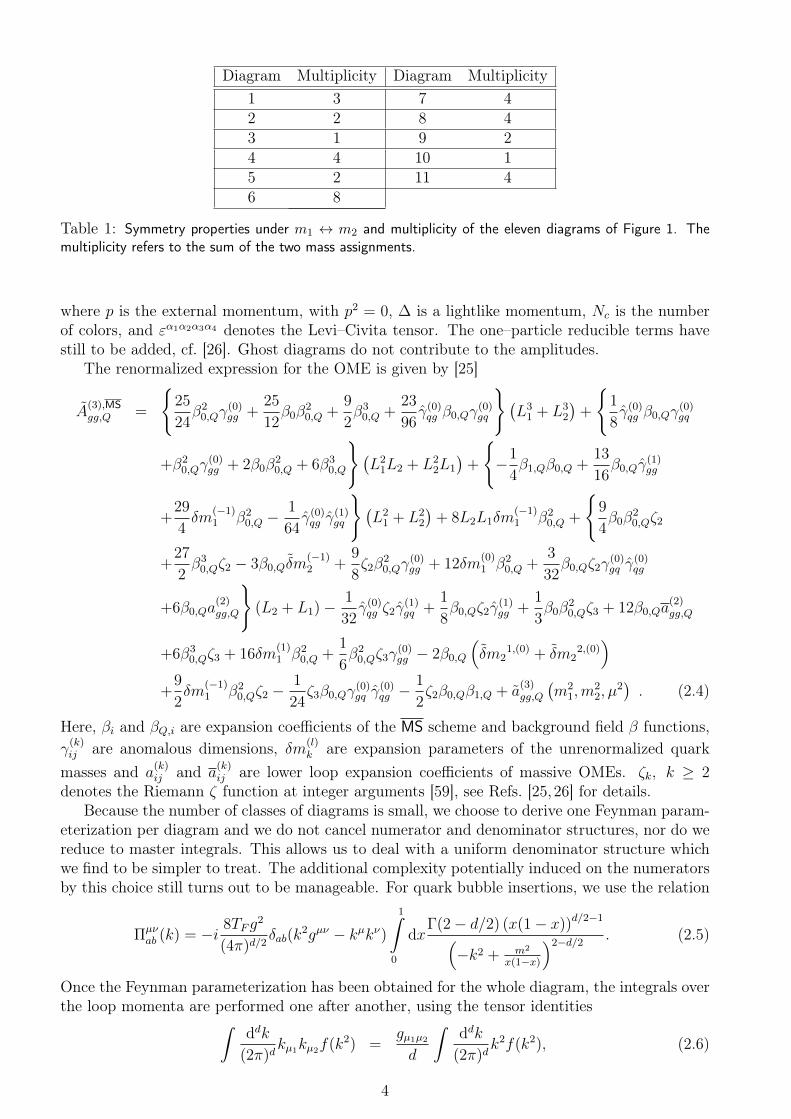
Diagram Multiplicity Diagram Multiplicity1 3 7 42 2 8 43 1 9 24 4 10 15 2 11 46 8

Table 1: Symmetry properties under m1 ↔ m2 and multiplicity of the eleven diagrams of Figure 1. Themultiplicity refers to the sum of the two mass assignments.

where p is the external momentum, with p2 = 0, ∆ is a lightlike momentum, Nc is the numberof colors, and εα1α2α3α4 denotes the Levi–Civita tensor. The one–particle reducible terms havestill to be added, cf. [26]. Ghost diagrams do not contribute to the amplitudes.

The renormalized expression for the OME is given by [25]

A(3),MSgg,Q =

{25

24β20,Qγ

(0)gg +

25

12β0β

20,Q +

9

2β30,Q +

23

96γ(0)qg β0,Qγ

(0)gq

}(L31 + L3

2

)+

{1

8γ(0)qg β0,Qγ

(0)gq

+β20,Qγ

(0)gg + 2β0β

20,Q + 6β3

0,Q

}(L21L2 + L2

2L1

)+

{−1

4β1,Qβ0,Q +

13

16β0,Qγ

(1)gg

+29

4δm

(−1)1 β2

0,Q −1

64γ(0)qg γ

(1)gq

}(L21 + L2

2

)+ 8L2L1δm

(−1)1 β2

0,Q +

{9

4β0β

20,Qζ2

+27

2β30,Qζ2 − 3β0,Qδm

(−1)2 +

9

8ζ2β

20,Qγ

(0)gg + 12δm

(0)1 β2

0,Q +3

32β0,Qζ2γ

(0)gq γ

(0)qg

+6β0,Qa(2)gg,Q

}(L2 + L1)−

1

32γ(0)qg ζ2γ

(1)gq +

1

8β0,Qζ2γ

(1)gg +

1

3β0β

20,Qζ3 + 12β0,Qa

(2)gg,Q

+6β30,Qζ3 + 16δm

(1)1 β2

0,Q +1

6β20,Qζ3γ

(0)gg − 2β0,Q

(δm2

1,(0) + δm22,(0))

+9

2δm

(−1)1 β2

0,Qζ2 −1

24ζ3β0,Qγ

(0)gq γ

(0)qg −

1

2ζ2β0,Qβ1,Q + a

(3)gg,Q

(m2

1,m22, µ

2). (2.4)

Here, βi and βQ,i are expansion coefficients of the MS scheme and background field β functions,γ(k)ij are anomalous dimensions, δm(l)

k are expansion parameters of the unrenormalized quarkmasses and a

(k)ij and a

(k)ij are lower loop expansion coefficients of massive OMEs. ζk, k ≥ 2

denotes the Riemann ζ function at integer arguments [59], see Refs. [25,26] for details.Because the number of classes of diagrams is small, we choose to derive one Feynman param-

eterization per diagram and we do not cancel numerator and denominator structures, nor do wereduce to master integrals. This allows us to deal with a uniform denominator structure whichwe find to be simpler to treat. The additional complexity potentially induced on the numeratorsby this choice still turns out to be manageable. For quark bubble insertions, we use the relation

Πµνab (k) = −i 8TFg

2

(4π)d/2δab(k

2gµν − kµkν)1∫

0

dxΓ(2− d/2) (x(1− x))d/2−1(−k2 + m2

x(1−x)

)2−d/2 . (2.5)

Once the Feynman parameterization has been obtained for the whole diagram, the integrals overthe loop momenta are performed one after another, using the tensor identities∫

ddk

(2π)dkµ1kµ2f(k2) =

gµ1µ2d

∫ddk

(2π)dk2f(k2), (2.6)

4

∫ddk

(2π)dkµ1kµ2kµ3kµ4f(k2) =

Sµ1µ2µ3µ4d(d+ 2)

∫ddk

(2π)d(k2)2f(k2),

(2.7)∫ddk

(2π)dkµ1kµ2kµ3kµ4kµ5kµ6f(k2) =

Sµ1µ2µ3µ4µ5µ6d(d+ 2)(d+ 4)

∫ddk

(2π)d(k2)3f(k2), (2.8)

with the symmetric tensors

Sµ1µ2µ3µ4 = gµ1µ2gµ3µ4 + gµ1µ3gµ2µ4 + gµ1µ4gµ2µ3 (2.9)Sµ1µ2µ3µ4µ5µ6 = gµ1µ2 [gµ3µ4gµ5µ6 + gµ3µ5gµ4µ6 + gµ3µ6gµ4µ5 ]

+gµ1µ3 [gµ2µ4gµ5µ6 + gµ2µ5gµ4µ6 + gµ2µ6gµ4µ5 ]

+gµ1µ4 [gµ2µ3gµ5µ6 + gµ2µ5gµ3µ6 + gµ2µ6gµ3µ5 ]

+gµ1µ5 [gµ2µ3gµ4µ6 + gµ2µ4gµ3µ6 + gµ2µ6gµ3µ4 ]

+gµ1µ6 [gµ2µ3gµ4µ5 + gµ2µ4gµ3µ5 + gµ2µ5gµ3µ4 ] . (2.10)

The scalar integrals can then be performed using the relation∫ddk

(2π)d(k2)m

(k2 +R2)n=

1

(4π)d/2Γ(n−m− d/2)

Γ(n)

Γ(m+ d/2)

Γ(d/2)

(R2)m−n+d/2

. (2.11)

After this step, only integrations over the Feynman parameters remain. They can always be castinto the form

j∏i=1

1∫0

dxi xaii (1− xi)bi RN

0

[R1 m

21 +R2 m

22

]−s, (2.12)

where R0 is a polynomial in the Feynman parameters xi, and R1 and R2 are rational functions inxi. At this point the polynomial R0 can be treated by applying the binomial theorem (multipletimes if necessary)

(A+B)N =N∑i=0

(N

i

)AiBN−i (2.13)

and a Mellin–Barnes decomposition [60–64] is applied to the factor [R1 m21 +R2 m

22]−s,

1

(A+B)s=

1

2πi

1

Γ(s)B−s

+i∞∫−i∞

dσ

(A

B

)σΓ(−σ)Γ(σ + s), (2.14)

where the integration contour must separate the ascending from the descending poles in theΓ–functions. After appropriately closing the contour at infinity, this integral is turned into anumber of infinite sums using the residue theorem. At this point the integrals over xi can alwaysbe expressed in terms of Beta functions.

The effect of these steps is to transform expressions having the form (2.12), i.e. integralsover Feynman parameters, into nested sums. This sum representation can be handled by Sigma,EvaluateMultiSums, SumProduction, assisted by HarmonicSums.

We checked our computation using the packages MB [65] and MBResolve [66] to resolve thesingularity structure of the Mellin–Barnes integrals numerically and to compute the ε-poles ofthe various diagrams for fixed values of N , and compared them to the general N results obtainedusing Sigma.

The target function space for the result is that of harmonic sums [36,37]

Sb,~a(N) =N∑k=1

(sign(b))k

k|b|S~a(k), ai, b ∈ Z\{0}, N ∈ N, S∅ = 1, (2.15)

5

generalized harmonic sums [38,47,67]

Sb,~a(d,~c)(N) =N∑k=1

dk

k|b|S~a(~c)(k), ai, b ∈ N\{0}, ci, d ∈ C(

√η)\{0}, N ∈ N, S∅ = 1, (2.16)

cyclotomic sums [39] and binomial sums [40]. Here the index d denotes a function of √η.Harmonic polylogarithms [48] will also appear in the result. The procedure adopted here is thesame as used in Ref. [25], where the corresponding unpolarized OME was computed. There, thereader can find further details and also explicit examples about the computational method.

The renormalization procedure is the same as in the unpolarized case, including the removalof collinear singularities, cf. [26].

All structures of the massive OME are predicted by the renormalization or are available fromlower loop results, except for the constant term in the two–mass case, a(3)gg,Q, of the unrenormalizedthree–loop OME.

First we turn to the calculation of fixed moments of this quantity.

3 Fixed moments of a(3)gg,Q

Here we present the results for the fixed moments N = 3 and 5 of the massive OME including thereducible contributions. They were computed using the packages Q2E/EXP [68, 69] up to O(η2)and O(η), respectively. In what follows we use the abbreviation

Lη = ln(η). (3.1)

The moments are given by

a(3)gg,Q(N = 3) = CFT

2F

{− 444341

11664+

(− 1031

18+

25L1

9+

25L2

9

)ζ2 −

220

81ζ3 −

22121

648L1

−5635

108L21 +

155

81L31 −

76411

1944L2 −

1822

27L1L2 +

10

27L21L2 −

5635

108L22

+50

27L1L

22 +

115

81L32 + η

(5528

675+

112

45Lη

)+ η2

(− 6202718

1157625+

32804

11025Lη

−116

105L2η

)}+ CAT

2F

{− 2146957

8748+

(− 3070

81− 560

9L1 −

560

9L2

)ζ2

+320

81ζ3 −

94403

486L1 −

3005

81L21 −

2320

81L31 −

16781

162L2 −

3200

81L1L2

−800

27L21L2 −

3005

81L22 −

1120

27L1L

22 −

2000

81L32 + η

(− 1869176

30375

+61346

2025Lη −

313

135L2η

)+ η2

(− 94073888

10418625+

486314

99225Lη −

1126

945L2η

)}+T 3

F

{(32L1 + 32L2

)ζ2 +

128

9ζ3 +

32

3L31 +

64

3L21L2 +

64

3L1L

22 +

32

3L32

}+O

(η3L3

η

), (3.2)

a(3)gg,Q(N = 5) = CFT

2F

{− 20217949

455625+

(− 12976

225+

56

45L1 +

56

45L2

)ζ2 −

2464

2025ζ3

−1202098

30375L1 −

177256

3375L21 +

1736

2025L31 −

411926

10125L2 −

229408

3375L1L2

+112

675L21L2 −

177256

3375L22 +

112

135L1L

22 +

1288

2025L32 + η

(52768

10125+

1984

675Lη

)}6

+CAT2F

{− 466789273

1366875+

(− 125176

2025− 3724

45L1 −

3724

45L2

)ζ2 +

2128

405ζ3

−2733284

10125L1 −

120092

2025L21 −

15428

405L31 −

4547582

30375L2 −

135344

2025L1L2

−1064

27L21L2 −

120092

2025L22 −

7448

135L1L

22 −

2660

81L32 + η

(− 21339914

253125

+73016

1875Lη −

11146

3375L2η

)}+ T 3

F

{(32L1 + 32L2

)ζ2 +

128

9ζ3 +

32

3L31

+64

3L21L2 +

64

3L1L

22 +

32

3L32

}+O

(η2L2

η

), (3.3)

where CF = (N2c −1)/(2Nc), TF = 1/2, CA = Nc for SU(Nc) and Nc = 3 in the case of QCD. The

calculational methods used in the packages Q2E/EXP are very different of those of the presentcalculation. Therefore, these results, in form of an expansion in η, can be used for comparison.

We have compared also the fixed moments of each diagram to their calculation at generalvalues of N . For diagrams 1–8 we also calculated the first moment.

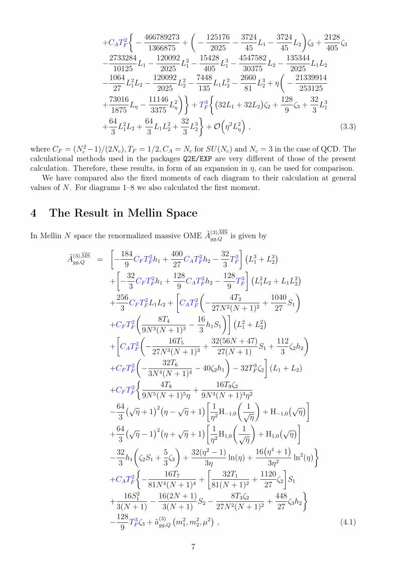
4 The Result in Mellin Space

In Mellin N space the renormalized massive OME A(3),MSgg,Q is given by

A(3),MSgg,Q =

[−184

9CFT

2Fh1 +

400

27CAT

2Fh2 −

32

3T 3F

] (L31 + L3

2

)+

[−32

3CFT

2Fh1 +

128

9CAT

2Fh2 −

128

9T 3F

] (L21L2 + L1L

22

)+

256

3CFT

2FL1L2 +

[CAT

2F

(− 4T2

27N2(N + 1)2+

1040

27S1

)+CFT

2F

(8T4

9N3(N + 1)3− 16

3h1S1

)] (L21 + L2

2

)+

[CAT

2F

(− 16T5

27N3(N + 1)3+

32(56N + 47)

27(N + 1)S1 +

112

3ζ2h2

)+CFT

2F

(− 32T6

3N4(N + 1)4− 40ζ2h1

)− 32T 3

F ζ2

](L1 + L2)

+CFT2F

{4T8

9N5(N + 1)5η+

16T9ζ29N3(N + 1)3η2

−64

3

(√η + 1

)2(η −√η + 1

)[ 1

η2H−1,0

(1√η

)+ H−1,0

(√η)]

+64

3

(√η − 1

)2(η +√η + 1

)[ 1

η2H1,0

(1√η

)+ H1,0

(√η)]

−32

3h1

(ζ2S1 +

5

3ζ3

)+

32(η2 − 1)

3ηln(η) +

16(η4 + 1

)3η2

ln2(η)

}+CAT

2F

{− 16T7

81N4(N + 1)4+

[32T1

81(N + 1)2+

1120

27ζ2

]S1

+16S2

1

3(N + 1)− 16(2N + 1)

3(N + 1)S2 −

8T3ζ227N2(N + 1)2

+448

27ζ3h2

}−128

9T 3F ζ3 + a

(3)gg,Q

(m2

1,m22, µ

2), (4.1)

7

where h1 and h2 are given by

h1 =(N − 1)(N + 2)

N2(N + 1)2, (4.2)

h2 = S1 −2

N(N + 1), (4.3)

and the polynomials Ti read

T1 = 328N2 + 584N + 283, (4.4)T2 = 171N4 + 342N3 + 847N2 + 676N − 156, (4.5)T3 = 99N4 + 198N3 + 463N2 + 364N − 84, (4.6)T4 = 66N6 + 198N5 + 169N4 + 80N3 + 140N2 − 47N − 78, (4.7)T5 = 15N6 + 45N5 + 374N4 + 601N3 + 161N2 − 24N + 36, (4.8)T6 = 2N8 + 8N7 + 18N6 + 20N5 + 2N4 − 3N2 − 9N − 6, (4.9)T7 = 3N8 + 12N7 + 2080N6 + 5568N5 + 4602N4 + 1138N3

−3N2 − 36N − 108, (4.10)T8 = −144η + 72η2N10 + 247ηN10 + 72N10 + 360η2N9 + 1235ηN9

+360N9 + 720η2N8 + 2182ηN8 + 720N8 + 720η2N7 + 1606ηN7

+720N7 + 360η2N6 + 875ηN6 + 360N6 + 72η2N5 + 1183ηN5

+72N5 + 1152ηN4 + 216ηN3 − 288ηN2 − 360ηN, (4.11)T9 = −42η2 − 36η7/2N6 − 36η5/2N6 − 36η3/2N6 + 12η4N6 + 57η2N6

−36√ηN6 + 12N6 − 108η7/2N5 − 108η5/2N5 − 108η3/2N5

+36η4N5 + 171η2N5 − 108√ηN5 + 36N5 − 108η7/2N4

−108η5/2N4 − 108η3/2N4 + 36η4N4 + 160η2N4 − 108√ηN4

+36N4 − 36η7/2N3 − 36η5/2N3 − 36η3/2N3 + 12η4N3 + 71η2N3

−36√ηN3 + 12N3 + 68η2N2 − 29η2N. (4.12)

Here, the functions H~a denote the harmonic polylogarithms [48]

Hb,~a(x) =

∫ x

0

dzfb(z)H~a(z), fb(z) ∈{f0 =

1

z, f1 =

1

1− z , f−1 =1

1 + z

}, H∅ = 1. (4.13)

Later also cyclotomic harmonic polylogarithms [39] will contribute. To account for their letters,a two–index structure is needed, e.g.

f4,0 =1

1 + x2, f4,1 =

x

1 + x2. (4.14)

The denominators are cyclotomic polynomials with p3 = 1 + x + x2, p4 = 1 + x2, p5 = 1 + x +x2 + x3 + x4, p6 = 1− x+ x2 etc. The maximal degree of the numerator for the kth cyclotomicdenominator polynomial is given by l = ϕ(k), where ϕ denotes Euler’s totient function.

All contributions except of the constant part of the unrenormalized OME, a(3)gg,Q (m21,m

22, µ

2),are predicted by the renormalization procedure, which provides a check of the present calculation.

The Mellin–Barnes and binomial representations of the individual Feynman diagrams implysum representations which can be summed using the technologies provided by the packagesSigma, EvaluateMultisums and SumProduction. Here we distinguish the cases of the realparameter η and 1/η. The computation time for the calculation amounted to several months.The solution is given in terms of harmonic sums, generalized harmonic sums and finite binomialand inverse binomial sums [40] over generalized sums.

8

In the following, whenever the argument of a harmonic polylogarithm is omitted, it is impliedto be η, and whenever the argument of a harmonic sum is omitted, it is implied to be N .

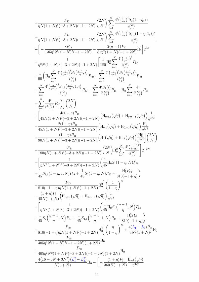
One obtains

a(3)gg,Q =

1

2

(1− (−1)N

){CFT

2F

{− L1L2P39

12ηN3(1 +N)3− 8(L1 + L2)P51

27N4(1 +N)4

+P59

243ηN5(1 +N)5(−3 + 2N)(−1 + 2N)− 5(η2 − 1)(L1 − L2)

2η

+16(N − 1)(2 +N)

(L21L2 + L1L

22

)N2(1 +N)2

+24(N − 1)(2 +N)

(L31 + L3

2

)N2(1 +N)2

+N − 1

N3(1 +N)2(−3 + 2N)(−1 + 2N)

[[8(2 +N)S2(1− η,N)P10

3η− 4H2

0P21

3η

−8H0S1(1− η,N)P21

3η− 8S1,1(1− η, 1, N)P21

3η

](1

1− η

)N+

[8

3(2 +N)S2

(η − 1

η,N)P8 −

4

3H2

0P15 +8

3H0S1

(η − 1

η,N)P15

−8

3S1,1

(η − 1

η, 1, N

)P15

](η

1− η

)N]+

(N − 1)(2 +N)

N2(1 +N)2

[128

3

(H0H0,1

−H0,0,1

)− 32

3

[S1

( 1

1− η ,N)

+ S1

( η

η − 1, N)]

H20 −

32

9H3

0

−64

3H2

0H1 +32

27S31 −

704

27S3 +

128

3S2,1

−64

3H0

[S1,1

( 1

1− η , 1− η,N)− S1,1

( η

η − 1,η − 1

η,N)]

+64

3

[S1,2

( 1

1− η , 1− η,N)

+ S1,2

( η

η − 1,η − 1

η,N)]

−64

3

[S1,1,1

( 1

1− η , 1− η, 1, N)

+ S1,1,1

( η

η − 1,η − 1

η, 1, N

)]−352

9ζ3

]+(L21 + L2

2

)( 5

8η+

5η

8− P36

12N3(1 +N)3

)+

N − 1

ηN(1 +N)2(−3 + 2N)(−1 + 2N)4N

(2N

N

)×[− 4

3(2 +N)

N∑i=1

4i(

11−η

)iS2(1− η, i)i(2ii

) P4 −4

3

N∑i=1

4i(

ηη−1

)iS1,1

(η−1η, 1, i

)i(2ii

) P7

−2

3H2

0

N∑i=1

4i(

ηη−1

)ii(2ii

) P7 −16

3(η − 1)H0

N∑i=1

4i

i2(2ii

)P9 −8

3

N∑i=1

4iS1(i)

i2(2ii

) P12

+8

3

N∑i=1

4i

i3(2ii

)P12 +2

3H2

0

N∑i=1

4i(

11−η

)ii(2ii

) P13

+4

3

((2 +N)

N∑i=1

4i(

ηη−1

)iS2

(η−1η, i)

i(2ii

) P1 + H0

N∑i=1

4i(

ηη−1

)iS1

(η−1η, i)

i(2ii

) P7

+H0

N∑i=1

4i(

11−η

)iS1(1− η, i)i(2ii

) P13 +N∑i=1

4i(

11−η

)iS1,1(1− η, 1, i)i(2ii

) P13

)]

9

+(1 + η)(N − 1)(2 +N)P2

3η3/2N(1 +N)2(−3 + 2N)(−1 + 2N)4N

(2N

N

)[− 16

(H0,0,1

(√η)

+ H0,0,−1(√

η))

+8(

H0,1

(√η)

+ H0,−1(√

η))

H0 − 2(

H1

(√η)

+ H−1(√

η))

H20

]+

8(5 + 8N)P24

9ηN(1 +N)2(−3 + 2N)(−1 + 2N)(1 + 2N)H0

+(1 + η)

(5− 2η + 5η2

)η3/2

[− 1

4(L1 − L2)

(H0,1

(√η)

+ H0,−1(√

η))

−1

2

(H0,0,1

(√η)

+ H0,0,−1(√

η))− 1

16(L1 − L2)

2(

H1

(√η)

+ H−1(√

η))]

− 8P55

9ηN3(1 +N)3(−3 + 2N)(−1 + 2N)(1 + 2N)H0

+32(N − 1)(2 +N)

(− 6− 8N +N2

)(L1 − L2)

3N3(1 +N)3H0

+48(N − 1)(2 +N)

(L21 − L2

2

)N2(1 +N)2

H0 +32(N − 1)(2 +N)

(− 6− 8N +N2

)3N3(1 +N)3

H20

+48(N − 1)(2 +N)(L1 + L2)

N2(1 +N)2H2

0 +

[− 16(N − 1)P49

81ηN4(1 +N)4(−3 + 2N)(−1 + 2N)

+32(N − 1)(2 +N)

(− 6− 8N +N2

)(L1 + L2)

9N3(1 +N)3+

16(N − 1)(2 +N)(L21 + L2

2

)N2(1 +N)2

+(N − 1)(2 +N)

N2(1 +N)2

(32(L1 − L2)H0 + 32H2

0 −32

3S2

)]S1

+32(N − 1)(2 +N)

(− 6− 8N +N2

)27N3(1 +N)3

S21 +

16(N − 1)(2 +N)(L1 + L2)

3N2(1 +N)2S21

−32(N − 1)(2 +N)(− 6− 8N +N2

)9N3(1 +N)3

S2 −16(N − 1)(2 +N)(L1 + L2)

N2(1 +N)2S2

+

[− 8P33

9N3(1 +N)3+

40(N − 1)(2 +N)(L1 + L2)

N2(1 +N)2+

32(N − 1)(2 +N)S1

3N2(1 +N)2

]ζ2

}+CAT

2F

{− 8L2

1L2

(− 8 +N +N2

)3N(1 +N)

− 16L1L22

(− 4 +N +N2

)3N(1 +N)

+40L3

2

(12 +N +N2

)9N(1 +N)

+32L3

1

(15 +N +N2

)9N(1 +N)

− L1L2P25

27ηN2(1 +N)2+

2(L1 + L2)P34

27N3(1 +N)3

+P50

18η3(1 +N)4(2 +N)4(−1 + 2N)(1 + 2N)

+P61

7290η3N4(1 +N)4(2 +N)4(−3 + 2N)(−1 + 2N)(1 + 2N)

−8(η2 − 1)(L1 − L2)

3η+

1

54

(L21 + L2

2

)(36

η+ 36η +

P18

N2(1 +N)2

)+(

H0,1

(√η)

+ H0,−1(√

η))[ (1 + η)P5

90N(1 +N)

H0

η3/2

−1

3(1 + η)

(4 + 11η + 4η2

)(L1 − L2)

1

η3/2

]+

[1

90

[P44

ηN(1 +N)2(−3 + 2N)(−1 + 2N)

(2N

N

)H0

N∑i=1

4i(

11−η

)iS1(1− η, i)i(2ii

)

10

+P42

ηN(1 +N)2(−3 + 2N)(−1 + 2N)

(2N

N

) N∑i=1

4i(

11−η

)iS2(1− η, i)i(2ii

)+

P44

ηN(1 +N)2(−3 + 2N)(−1 + 2N)

(2N

N

) N∑i=1

4i(

11−η

)iS1,1(1− η, 1, i)i(2ii

) ]+

[− 8P28

135η2N(1 +N)2(−1 + 2N)− 2(η − 1)P27

81η2(1 +N)(−1 + 2N)H0

]22N

+1

η2N(1 +N)2(−3 + 2N)(−1 + 2N)

[1

180H2

0

N∑i=1

4i(

ηη−1

)ii(2ii

) P37

+1

90

(H0

N∑i=1

4i(

ηη−1

)iS1

(η−1η, i)

i(2ii

) P30 +N∑i=1

4i(

ηη−1

)iS2

(η−1η, i)

i(2ii

) P30

+N∑i=1

4i(

ηη−1

)iS1,1

(η−1η, 1, i

)i(2ii

) P37 +N∑i=1

4iS1(i)

i2(2ii

) P45 + H0

N∑i=1

4i

i2(2ii

)P46

+N∑i=1

4i

i3(2ii

)P47

)](2N

N

)+

[4(1 + η)P41

45N(1 +N)2(−3 + 2N)(−1 + 2N)

(H0,0,1

(√η)

+ H0,0,−1(√

η)) 1

η3/2

− 2(1 + η)P41

45N(1 +N)2(−3 + 2N)(−1 + 2N)

(H0,1

(√η)

+ H0,−1(√

η)) H0

η3/2

+(1 + η)P41

90N(1 +N)2(−3 + 2N)(−1 + 2N)

(H1

(√η)

+ H−1(√

η)) H2

0

η3/2

](2N

N

)+

P44

180ηN(1 +N)2(−3 + 2N)(−1 + 2N)

(2N

N

)H2

0

N∑i=1

4i(

11−η

)ii(2ii

) ]2−2N

+

[1

ηN2(1 +N)2(−3 + 2N)(−1 + 2N)

(1

45H0S1(1− η,N)P38

+1

45S1,1(1− η, 1, N)P38 +

1

45S2(1− η,N)P40 +

H20P56

810(−1 + η)

)+

P43

810(−1 + η)ηN(1 +N)2(−1 + 2N)H2

0

](1

1− η

)N− (1 + η)P6

45N(1 +N)

(H0,0,1

(√η)

+ H0,0,−1(√

η)) 1

η3/2

+

[1

ηN2(1 +N)2(−3 + 2N)(−1 + 2N)

(1

45H0S1

(η − 1

η,N)P31

+1

45S2

(η − 1

η,N)P31 +

1

45S1,1

(η − 1

η, 1, N

)P35 +

H20P52

810(−1 + η)

)+

P32

810(−1 + η)ηN(1 +N)2(−1 + 2N)H2

0

](η

1− η

)N+

4(L1 − L2)P16

9N2(1 +N)2H0

+P48

405η2N(1 +N)3(−1 + 2N)(1 + 2N)H0

+P58

405η2N2(1 +N)3(−3 + 2N)(−1 + 2N)(1 + 2N)H0

+4(16 + 3N + 3N2

)(L21 − L2

2

)N(1 +N)

H0 +

[− (1 + η)P5

360N(1 +N)

H−1(√

η)

η3/2

11

+P26

180ηN2(1 +N)2+

8(16 + 3N + 3N2

)(L1 + L2)

3N(1 +N)

]H2

0 −4(16 + 3N + 3N2

)27N(1 +N)

H30

+

[8

3

(L21 − 2L1L2 + L2

2

)− 8

(16 + 3N + 3N2

)9N(1 +N)

H20

]H1

+

[− (1 + η)

360N(1 +N)

H20

η3/2P5 −

1

12(1 + η)

(4 + 11η + 4η2

)(L1 − L2)

2 1

η3/2

]H1

(√η)

− 1

12(1 + η)

(4 + 11η + 4η2

)(L1 − L2)

2H−1(√

η)

η3/2+

[16

3(L1 − L2)

+16(16 + 3N + 3N2

)9N(1 +N)

H0

]H0,1 −

256H0,0,1

9N(1 +N)

+2P19

135η2N(1 +N)3(−1 + 2N)S1 +

[− 640L1L2

27+

8H0ζ2P22

45ηN2(1 +N)2

+8H0P23

45ηN2(1 +N)2− 8(L1 + L2)P17

27N2(1 +N)2+

2P57

3645η2N3(1 +N)3(−3 + 2N)(−1 + 2N)

−32

3L1L2(L1 + L2)−

1360

27

(L21 + L2

2

)− 80

3

(L31 + L3

2

)−8

9(1 + η)

(5 + 22η + 5η2

)(H0,0,1

(√η)

+ H0,0,−1(√

η)) 1

η3/2

−8(− 93 + 37N + 46N2

)(L1 − L2)

9N(1 +N)H0 − 32

(L21 − L2

2

)H0

+4

9(1 + η)

(5 + 22η + 5η2

)(H0,1

(√η)

+ H0,−1(√

η)) H0

η3/2+

[2P3

9ηN(1 +N)

−64

3(L1 + L2)−

1

9(1 + η)

(5 + 22η + 5η2

)H−1(√

η)

η3/2

]H2

0 +32

27H3

0

+64

9H2

0H1 −1

9(1 + η)

(5 + 22η + 5η2

)H20H1

(√η)

η3/2− 128

9H0H0,1

+128

9H0,0,1 −

64L2

3ζ2 +

2P53

3645η2N3(1 +N)3(−3 + 2N)(−1 + 2N)ζ2

]S1

+

[− 4P11

135ηN2(1 +N)2− 16

3(L1 − L2)H0 −

16

3H2

0

]S21

+

[− 4P20

135ηN2(1 +N)2+

16

15η(1 +N)

(− 8 + 8η2 − 4N + 4η2N

)H0

−16(L1 − L2)H0 − 16H20

]S2 −

64

15η(1 +N)

(2 + 2η2 +N + η2N

)S3

+64

15η(1 +N)

(2 + 2η2 +N + η2N

)S2,1 −

32(2η + ηN)

15(1 +N)H2

0S1

( 1

1− η ,N)

−32(2 +N)H2

0S1

(ηη−1 , N

)15η(1 +N)

− 64(2η + ηN)

15(1 +N)H0S1,1

( 1

1− η , 1− η,N)

+64(2 +N)H0S1,1

(ηη−1 ,

η−1η, N)

15η(1 +N)+

64(2η + ηN)

15(1 +N)S1,2

( 1

1− η , 1− η,N)

+64(2 +N)S1,2

(ηη−1 ,

η−1η, N)

15η(1 +N)− 64(2η + ηN)

15(1 +N)S1,1,1

( 1

1− η , 1− η, 1, N)

−64(2 +N)S1,1,1

(ηη−1 ,

η−1η, 1, N

)15η(1 +N)

+8L2P29

3N(1 +N)(−3 + 2N)(−1 + 2N)(1 + 2N)ζ2

12

+P60

7290η3N4(1 +N)4(2 +N)4(−3 + 2N)(−1 + 2N)(1 + 2N)ζ2 +

[224L1

3N(1 +N)

− 4P14

27N2(1 +N)2− 8L2

(20 + 15N + 7N2

)3N(1 +N)

+4(48 + 15N + 7N2

)3N(1 +N)

H0

+

[− 112L1

3− 16L2 −

16(− 69 + 38N + 47N2

)27N(1 +N)

− 32

3H0

]S1

]ζ2

+P54

405η2N2(1 +N)3(−3 + 2N)(−1 + 2N)(1 + 2N)H0ζ2 +

[− 128

27N(1 +N)

+64

27S1

]ζ3

}+ T 3

F

{32

3

(L31 + 2L2

1L2 + 2L1L22 + L3

2

)+ 32(L1 + L2)ζ2 +

128

9ζ3

}},

(4.15)

where the polynomials Pi are

P1 = −27− 36N2 − 36N(−2 + η) + 54η + 5η2 (4.16)P2 = 5− 2

(− 11− 18N + 18N2

)η + 5η2 (4.17)

P3 = 372η +N2(5− 102η + 5η2

)+N

(5− 66η + 5η2

)(4.18)

P4 = −5 + 18(−3 + 2N)η + 9(−3 + 2N)(−1 + 2N)η2 (4.19)P5 = −80

(5 + 22η + 5η2

)+ 3N2

(71− 46η + 71η2

)+ 3N

(167 + 18η + 167η2

)(4.20)

P6 = −80(5 + 22η + 5η2

)+ 3N2

(111 + 64η + 111η2

)+ 3N

(207 + 128η + 207η2

)(4.21)

P7 = −(2 +N)[27 + 36N2 + 36N(−2 + η)− 54η − 5η2

](4.22)

P8 = 24− 48N − 18N3 + 5N2(9 + η) (4.23)P9 = (2 +N)(−4 + 3N)(−2 + 3N)(1 + η) (4.24)P10 = −24η + 48Nη + 18N3η − 5N2(1 + 9η) (4.25)P11 = 9 + 160η + 50N2η + 140N3η + 9η2 − 9N

(7 + 10η + 7η2

)(4.26)

P12 = (2 +N)[11− 54η + 11η2 + 18N2

(1 + η2

)− 36N

(1− η + η2

)](4.27)

P13 = (2 +N)[− 5 + 18(−3 + 2N)η + 9(−3 + 2N)(−1 + 2N)η2

](4.28)

P14 = 168− 536N − 407N2 − 278N3 − 167N4 (4.29)

P15 = −(2 +N)[− 24 + 48N + 18N3 − 5N2(9 + η)

](4.30)

P16 = −96 + 370N + 277N2 + 12N3 + 9N4 (4.31)P17 = 48− 27N + 263N2 + 634N3 + 344N4 (4.32)P18 = −1632 + 7072N + 8611N2 + 3078N3 + 1539N4 (4.33)P19 = −20N4(10 + 81η)− 4N3

(41 + 855η + 135η2

)+N

(41 + 855η − 765η2 − 87η3

)−3(17 + 60η − 135η2 + 2η3

)+N2

(254 + 1125η + 180η2 + 45η3

)(4.34)

P20 = 50N2η − 660N3η − 440N4η − 3(3 + 160η + 3η2

)+ 9N

(7 + 30η + 7η2

)(4.35)

P21 = (2 +N)[− 24η + 48Nη + 18N3η − 5N2(1 + 9η)

](4.36)

P22 = 60N2(1 +N)2η (4.37)P23 =

(3− 21N + 25N2 + 50N3 + 25N4

)(−1 + η)(1 + η) (4.38)

P24 = −36N3(−1 + η)η + 36N4η2 +N(1 + 15η)(−5 + 21η)− 4(5 + 27η2

)−N2

(5 + 18η + 189η2

)(4.39)

P25 = 384η − 1664Nη + 18N3(4− 93η + 4η2

)+ 9N4

(4− 93η + 4η2

)+N2

(36− 2501η + 36η2

)(4.40)

13

P26 = −48(1 + 160η + η2

)− 16N

(4− 1405η + 4η2

)+ 3N4

(71 + 134η + 71η2

)+N2

(101 + 15234η + 101η2

)+ 2N3

(357 + 418η + 357η2

)(4.41)

P27 = 56N4(1 + η)(1 + η2

)− 6(1 + η)

(5 + 86η + 5η2

)−N(1 + η)

(41 + 390η + 41η2

)+4N3(1 + η)

(41 + 405η + 41η2

)+ 2N2(1 + η)

(53 + 972η + 53η2

)(4.42)

P28 = 3(17 + 62η − 270η2 + 62η3 + 17η4

)+ 20N4

(10 + 81η + 81η3 + 10η4

)−N

(41 + 768η − 1530η2 + 768η3 + 41η4

)+4N3

(41 + 855η + 270η2 + 855η3 + 41η4

)−2N2

(127 + 585η + 180η2 + 585η3 + 127η4

)(4.43)

P29 = 144− 51N − 585N2 + 190N3 + 36N4 + 56N5 (4.44)P30 = −800N6 − 8N5(169 + 270η) + 4N4

(599− 645η + 30η2

)− 2N3

(− 1565− 3810η

+225η2 + 6η3)

+ 3N2(− 355 + 2255η + 335η2 + 53η3

)+3(43 + 705η + 405η2 + 175η3

)− 2N

(349 + 4530η + 855η2 + 342η3

)(4.45)

P31 = −400N6 + 24η(80 + 3η)− 4N5(119 + 128η) +N3(847 + 2314η − 513η2

)+N

(129− 4882η − 171η2

)− 4N4

(− 359 + 172η + 3η2

)+4N2

(− 239 + 572η + 189η2

)(4.46)

P32 = −280N6 − 100N5(11 + 81η) +N3(13967 + 41445η − 1755η2 − 2325η3

)+27

(− 61− 160η − 45η2 + 2η3

)− 90N4

(− 65− 72η + 27η2 + 20η3

)+N2

(5143 + 15660η − 405η2 + 174η3

)+3N

(− 1141− 3285η + 1125η2 + 377η3

)(4.47)

P33 = 2(− 42− 29N + 68N2 + 47N3 + 88N4 + 99N5 + 33N6

)(4.48)

P34 = 528− 224N + 2008N2 + 7149N3 + 4239N4 + 279N5 + 93N6 (4.49)P35 = 400N6 − 24η(80 + 3η) + 4N5(119 + 128η) + 4N4

(− 359 + 172η + 3η2

)+N

(− 129 + 4882η + 171η2

)− 4N2

(− 239 + 572η + 189η2

)+N3

(− 847− 2314η + 513η2

)(4.50)

P36 = −1088− 800N + 1664N2 + 1081N3 + 1675N4 + 1899N5 + 633N6 (4.51)P37 = 800N6 + 8N5(169 + 270η)− 4N4

(599− 645η + 30η2

)+ 2N3

(− 1565− 3810η

+225η2 + 6η3)− 3N2

(− 355 + 2255η + 335η2 + 53η3

)−3(43 + 705η + 405η2 + 175η3

)+ 2N

(349 + 4530η + 855η2 + 342η3

)(4.52)

P38 = −400N6η2 + 24(3 + 80η)− 4N5η(128 + 119η) +N(− 171− 4882η + 129η2

)−4N2

(− 189− 572η + 239η2

)+ 4N4

(− 3− 172η + 359η2

)+N3

(− 513 + 2314η + 847η2

)(4.53)

P39 = −512η − 256Nη + 1024N2η + 3N3(5 + 282η + 5η2

)+ 9N5

(5 + 282η + 5η2

)+3N6

(5 + 282η + 5η2

)+N4

(45 + 2282η + 45η2

)(4.54)

P40 = 400N6η2 − 24(3 + 80η) + 4N5η(128 + 119η) +N3(513− 2314η − 847η2

)+N

(171 + 4882η − 129η2

)+ 4N2

(− 189− 572η + 239η2

)−4N4

(− 3− 172η + 359η2

)(4.55)

P41 = 400N6(1− η + η2

)− 3(109 + 446η + 109η2

)+ 3N2

(151− 1446η + 151η2

)+4N5

(169 + 101η + 169η2

)− 2N4

(599− 1214η + 599η2

)+N

(691 + 4694η + 691η2

)−N3

(1559 + 2026η + 1559η2

)(4.56)

P42 = −800N6η3 − 8N5η2(270 + 169η) + 4N4η(30− 645η + 599η2

)+3N2

(53 + 335η + 2255η2 − 355η3

)+ 3(175 + 405η + 705η2 + 43η3

)−2N

(342 + 855η + 4530η2 + 349η3

)+ 2N3

(− 6− 225η + 3810η2 + 1565η3

)(4.57)

14

P43 = −280N6η3 − 100N5η2(81 + 11η)− 27(− 2 + 45η + 160η2 + 61η3

)+90N4

(− 20− 27η + 72η2 + 65η3

)− 3N

(− 377− 1125η + 3285η2 + 1141η3

)+N2

(174− 405η + 15660η2 + 5143η3

)+N3

(− 2325− 1755η + 41445η2 + 13967η3

)(4.58)

P44 = 800N6η3 + 8N5η2(270 + 169η)− 4N4η(30− 645η + 599η2

)−3(175 + 405η + 705η2 + 43η3

)+ 2N

(342 + 855η + 4530η2 + 349η3

)+3N2

(− 53− 335η − 2255η2 + 355η3

)− 2N3

(− 6− 225η + 3810η2 + 1565η3

)(4.59)

P45 = −800N6(1 + η4

)+ 3(43 + 880η + 810η2 + 880η3 + 43η4

)+N3

(3130 + 7608η − 900η2 + 7608η3 + 3130η4

)− 8N5

(169 + 270η + 270η3 + 169η4

)−2N

(349 + 4872η + 1710η2 + 4872η3 + 349η4

)−3N2

(355− 2308η − 670η2 − 2308η3 + 355η4

)+4N4

(599− 645η + 60η2 − 645η3 + 599η4

)(4.60)

P46 = −800N6(−1 + η)(1 + η)(1 + η2

)− 698N(−1 + η)(1 + η)

(1 + 12η + η2

)+3(−1 + η)(1 + η)

(43 + 530η + 43η2

)− 8N5(−1 + η)(1 + η)

(169 + 270η + 169η2

)−3N2(−1 + η)(1 + η)

(355− 2202η + 355η2

)+4N4(−1 + η)(1 + η)

(599− 645η + 599η2

)+2N3(−1 + η)(1 + η)

(1565 + 3816η + 1565η2

)(4.61)

P47 = 800N6(1 + η4

)− 3(43 + 880η + 810η2 + 880η3 + 43η4

)+N

(698 + 9744η + 3420η2 + 9744η3 + 698η4

)+ 8N5

(169 + 270η + 270η3 + 169η4

)+3N2

(355− 2308η − 670η2 − 2308η3 + 355η4

)−4N4

(599− 645η + 60η2 − 645η3 + 599η4

)−2N3

(1565 + 3804η − 450η2 + 3804η3 + 1565η4

)(4.62)

P48 = −560N7 − 40N6(62 + 405η) + 20N5(− 190− 2187η + 729η2

)+N2

(1417 + 12690η − 5535η2 − 240η3

)− 9(17 + 60η − 135η2 + 2η3

)+10N4

(− 260− 3807η + 2430η2 + 15η3

)−N3

(107 + 9045η − 4455η2 + 75η3

)−3N

(− 91− 1665η + 1575η2 + 137η3

)(4.63)

P49 = −(2 +N)[− 216η − 144Nη − 696N2η + 148N6η − 30N4

(9− 16η + 9η2

)−9N5

(15− 38η + 15η2

)−N3

(135 + 1022η + 135η2

)](4.64)

P50 = 225 + 1630η + 3456η2 + 2466η3 + 415η4

+N(930 + 5372η + 6912η2 + 2820η3 + 350η4

)−152N6η(1 + η)

(5 + 22η + 5η2

)− 16N7η(1 + η)

(5 + 22η + 5η2

)−192N3

(− 5 + 3η + 135η2 + 157η3 + 30η4

)−72N4

(− 5 + 53η + 405η2 + 427η3 + 80η4

)−12N5

(− 5 + 218η + 1296η2 + 1318η3 + 245η4

)− 6N2

(− 225− 830η

+864η2 + 1854η3 + 385η4)

(4.65)P51 = 396 + 690N + 518N2 + 240N3 − 289N4 − 432N5 + 494N6 + 588N7 + 147N8 (4.66)P52 = 560N8 − 216(−1 + η)η(80 + 3η) + 40N7(34 + 405η) +N4

(44539 + 73899η

+1629η2 − 7215η3)

+ 60N6(− 310− 561η + 81η2 + 60η3

)+9N

(− 420− 6451η + 4306η2 + 189η3

)− 2N5

(7334 + 31887η − 414η2 + 375η3

)−9N2

(1731− 919η + 137η2 + 391η3

)+ 3N3

(9966 + 26631η − 11136η2 + 959η3

)(4.67)

P53 = −1080N2(1 +N)2η2(207− 456N + 89N2 − 56N3 + 92N4

)(4.68)

P54 = −540N(1 +N)2η2(144− 51N − 585N2 + 190N3 + 36N4 + 56N5

)(4.69)

15

P55 = N2(1 +N)[288N5η2 − 36N4η(−8 + 3η)− 160

(1 + 3η2

)− 4N3

(− 5− 9η + 438η2

)+N

(− 275− 270η + 801η2

)+N2

(25− 522η + 1485η2

)](4.70)

P56 = 560N8η3 + 40N7η2(405 + 34η) + 216(−1 + η)(3 + 80η)− 60N6(− 60

−81η + 561η2 + 310η3)− 9N

(− 189− 4306η + 6451η2 + 420η3

)−9N2

(391 + 137η − 919η2 + 1731η3

)− 2N5

(375− 414η + 31887η2 + 7334η3

)+3N3

(959− 11136η + 26631η2 + 9966η3

)+N4

(− 7215 + 1629η + 73899η2 + 44539η3

)(4.71)

P57 = −51840η2 + 103680Nη2 + 80N8η(405− 10412η + 405η2

)−4N7

(− 2700− 20331η + 165688η2 + 1539η3

)−36N6

(204 + 378η − 49156η2 + 1863η3

)−9N2

(459 + 5184η + 20987η2 + 3618η3

)−2N5

(13500 + 171477η − 942766η2 + 3807η3

)−3N3

(− 2025− 24489η + 185329η2 + 4077η3

)+N4

(18360 + 94851η + 70490η2 + 58239η3

)(4.72)

P58 = N[2240N9(−1 + η)(1 + η)

(1 + η2

)+N4

(6264 + 156159η + 63990η2

−251679η3 − 13850 η4)

+N3(− 6175− 104082η + 24435η2 + 51822η3 + 3020η4

)+N2

(− 525− 58899η − 7155η2 + 87081η3 + 4230η4

)+ 27

(− 17− 96η + 135η2

+34η3)

+ 160N8(− 48− 405η + 405η3 + 55η4

)+8N7

(− 450− 13887η + 17937η3 + 860η4

)+9N

(25− 482η − 1845η2 + 2134η3 + 100η4

)−10N5

(− 2214− 30615η + 486η2 + 36153η3 + 2834η4

)−4N6

(− 3660− 21279η + 7290η2 + 11559η3 + 3620η4

)](4.73)

P59 = 36288η − 19872Nη − 220032N2η − 252192N3η +N5(− 61155 + 394298η − 61155η2

)+N6

(− 17415 + 597938η − 17415η2

)− 320N4

(81 + 526η + 81η2

)+36N11

(405− 3766η + 405η2

)+ 12N12

(405− 3766η + 405η2

)−5N9

(3483− 56554η + 3483η2

)+N10

(3645 + 44314η + 3645η2

)+10N7

(4455− 2386η + 4455η2

)+ 2N8

(7695− 64514η + 7695η2

)(4.74)

P60 = 1080N3(1 +N)2(2 +N)4η3(576 + 1173N − 2988N2 − 4835N3 + 2674N4 + 572N5

+248N6)

(4.75)P61 = −5806080η3 − 7464960Nη3 + 39628800N2η3

+N4(273375− 2809566η + 5935680η2 + 522717086η3 + 2240865η4 − 4790016η5

)+864N15η

(400 + 3639η + 589η2 + 3639η3 + 400η4

)−768N3η

(1377 + 4293η − 244034η2 + 4293η3 + 1377η4

)+432N14η

(7856 + 80679η + 16689η2 + 80679η3 + 7856η4

)−16N11η

(450738− 6962355η − 48003782η2 − 6819795η3 + 483138η4

)+8N13η

(1570752 + 18898191η + 7445585η2 + 18898191η3 + 1570752η4

)+4N12η

(4566888 + 73693719η + 72807653η2 + 73622439η3 + 4550688η4

)+4N5

(236925 + 975942η + 27088992η2 + 117199930η3 + 25711587η4 − 325728η5

)−12N8

(28350 + 912078η + 59340789η2 + 250807007η3 + 58332339η4 + 564588η5

)−36N9

(6075 + 1870314η + 30831858η2 + 19135996η3 + 30932703η4 + 1867884η5

)−8N10

(6075 + 7288137η + 73658484η2 − 103483664η3 + 74427579η4 + 7437582η5

)16

+4N7(18225 + 8623746η + 9768924η2 − 816997534η3 + 15310539η4 + 9807156η5

)+2N6

(443475 + 12987162η + 132854256η2 − 575608138η3 + 137257821η4

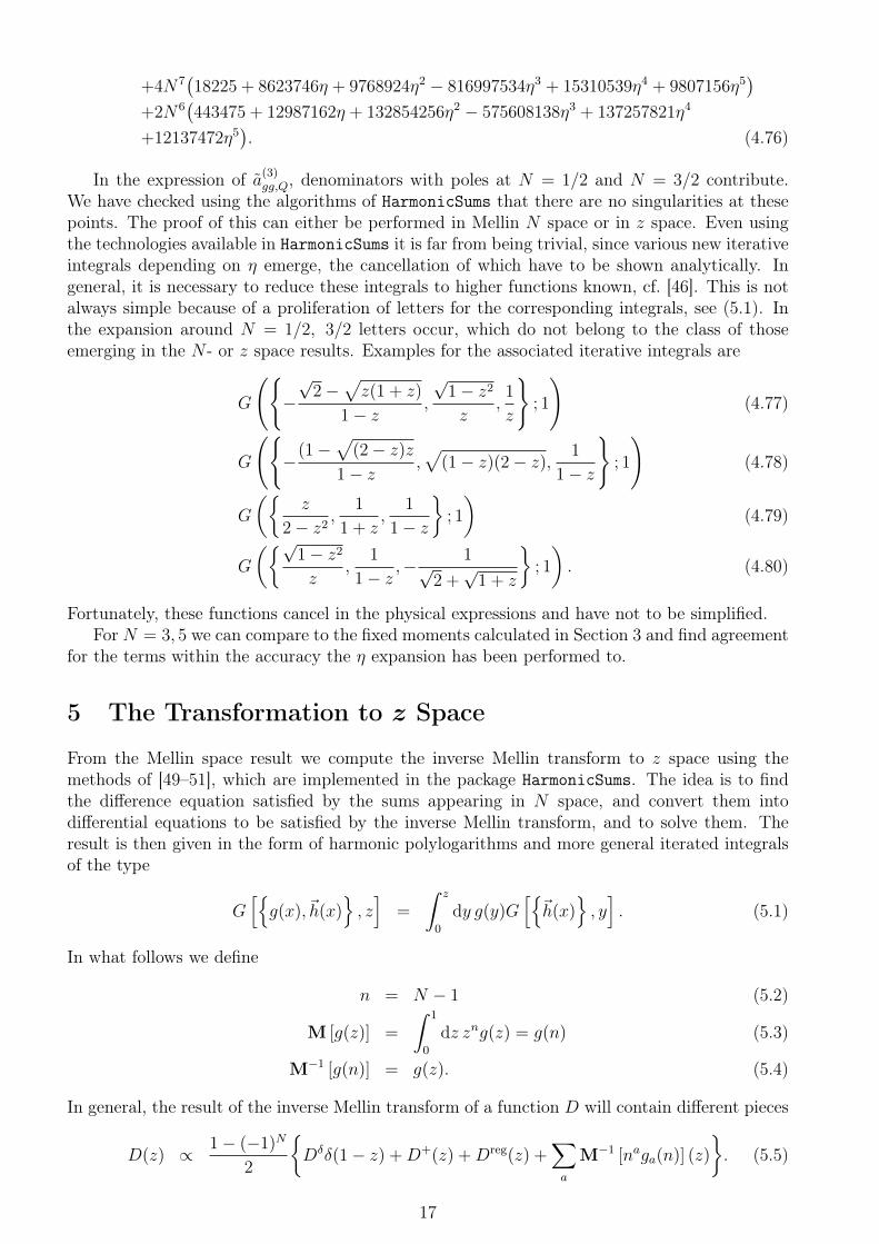
+12137472η5). (4.76)

In the expression of a(3)gg,Q, denominators with poles at N = 1/2 and N = 3/2 contribute.We have checked using the algorithms of HarmonicSums that there are no singularities at thesepoints. The proof of this can either be performed in Mellin N space or in z space. Even usingthe technologies available in HarmonicSums it is far from being trivial, since various new iterativeintegrals depending on η emerge, the cancellation of which have to be shown analytically. Ingeneral, it is necessary to reduce these integrals to higher functions known, cf. [46]. This is notalways simple because of a proliferation of letters for the corresponding integrals, see (5.1). Inthe expansion around N = 1/2, 3/2 letters occur, which do not belong to the class of thoseemerging in the N - or z space results. Examples for the associated iterative integrals are

G

({−√

2−√z(1 + z)

1− z ,

√1− z2z

,1

z

}; 1

)(4.77)

G

({−(1−

√(2− z)z

1− z ,√

(1− z)(2− z),1

1− z

}; 1

)(4.78)

G

({z

2− z2 ,1

1 + z,

1

1− z

}; 1

)(4.79)

G

({√1− z2z

,1

1− z ,−1√

2 +√

1 + z

}; 1

). (4.80)

Fortunately, these functions cancel in the physical expressions and have not to be simplified.For N = 3, 5 we can compare to the fixed moments calculated in Section 3 and find agreement

for the terms within the accuracy the η expansion has been performed to.

5 The Transformation to z Space

From the Mellin space result we compute the inverse Mellin transform to z space using themethods of [49–51], which are implemented in the package HarmonicSums. The idea is to findthe difference equation satisfied by the sums appearing in N space, and convert them intodifferential equations to be satisfied by the inverse Mellin transform, and to solve them. Theresult is then given in the form of harmonic polylogarithms and more general iterated integralsof the type

G[{g(x),~h(x)

}, z]

=

∫ z

0

dy g(y)G[{~h(x)

}, y]. (5.1)

In what follows we define

n = N − 1 (5.2)

M [g(z)] =

∫ 1

0

dz zng(z) = g(n) (5.3)

M−1 [g(n)] = g(z). (5.4)

In general, the result of the inverse Mellin transform of a function D will contain different pieces

D(z) ∝ 1− (−1)N

2

{Dδδ(1− z) +D+(z) +Dreg(z) +

∑a

M−1 [naga(n)] (z)

}. (5.5)

17

One distinguishes between the distribution Dδ, D+, and Dreg, the regular part, where Dδ is afunction of η and D+ is a +-distribution,∫ 1

0

dz g(z)(f(z)

)+

=

∫ 1

0

dz(g(z)− g(1)

)f(z), (5.6)

the regular part in z, Dreg. At times, it is necessary to absorb from the output of HarmonicSumsa rational pre–factor in n after applying a partial fractioning of the result, using the relations

1

(n+ a)i

∫ 1

0

dz zn f(z) =

∫ 1

0

dz zn{∫ 1

z

dy (−1)i−1(yz

)a [H0

(yz

)]i−1f(y)

}(5.7)

n

∫ 1

0

dz zn f(z) = (zn − 1)zf(z)|10 −∫ 1

0

(zn − 1)d

dz(zf(z)) . (5.8)

We denote the Mellin convolution by ⊗

f(z)⊗ g(z) =

∫ 1

0

dz1

∫ 1

0

dz2 δ(z − z1z2)f(z1)g(z2) (5.9)

for regular functions and, cf. [40],

[f(z)]+ ⊗ g(z) =

∫ 1

z

dy f(y)

[1

yg

(z

y

)− g(z)

]− g(z)

∫ z

0

dy f(y) (5.10)

for the Mellin convolution of a +-distribution and a regular function.Now we turn to a(3)gg,Q(z), which we represent in terms of the three contributing parts com-

bining to

a(3)gg,Q(N) =

∫ 1

0

dz zN−1 δ(1− z) a(3),δgg,Q(z) +

∫ 1

0

dz(zN−1 − 1

)a(3),+gg,Q (z)

+

∫ 1

0

dz zN−1 a(3),reggg,Q (z) . (5.11)

The result is expressed in terms of the iterated integrals Gi and the constants Ki defined inAppendix D of [25]. In the following the argument of the functions Gi is implied to be z in theformulas for a(3),δgg,Q(z), a(3),+gg,Q (z) and a(3),reggg,Q (z), and it is implied to be y in the functions Φi whichfollow. Such arguments are omitted in the interest of brevity. One finds

a(3),δgg,Q(z) = T 3

F

{32

3(L3

1 + L32) +

64

3(L2

1L2 + L1L22) + 32ζ2(L1 + L2) +

128

9ζ3

}+CFT

2F

{405− 3766η + 405η2

81η+ L1L2

[−5− 282η − 5η2

4η

+1

8(1 + η)

(5− 2η + 5η2

)(H1

(√η)

+ H−1(√

η)) 1

η3/2

]+(L2

1 + L22)

[5− 422η + 5η2

8η

− 1

16(1 + η)

(5− 2η + 5η2

)(H1

(√η)

+ H−1(√

η)) 1

η3/2

]+L1

[45− 784η − 45η2

18η

−1

4(1 + η)

(5− 2η + 5η2

)(H0,1

(√η)

+ H0,−1(√

η)) 1

η3/2

]18

+L2

[−45− 784η + 45η2

18η

+1

4(1 + η)

(5− 2η + 5η2

)(H0,1

(√η)

+ H0,−1(√

η)) 1

η3/2

]−1

2(1 + η)

(5− 2η + 5η2

)(H0,0,1

(√η)

+ H0,0,−1(√

η)) 1

η3/2− 176

3ζ2

}+CAT

2F

{38(21 + 31η + 21η2

)135η

+32L3

1

9− 8L2

1L2

3− 16L1L

22

3+

40L32

9

+L1L2

[−4 + 93η − 4η2

3η+

1

6(1 + η)

(4 + 11η + 4η2

)(H1

(√η)

+ H−1(√

η)) 1

η3/2

−16

3H1(η)

]+ L2

2

[4 + 171η + 4η2

6η

− 1

12(1 + η)

(4 + 11η + 4η2

)(H1

(√η)

+ H−1(√

η)) 1

η3/2− 12H0(η) +

8

3H1(η)

]+L2

1

[4 + 171η + 4η2

6η− 1

12(1 + η)

(4 + 11η + 4η2

)(H1

(√η)

+ H−1(√

η)) 1

η3/2

+12H0(η) +8

3H1(η)

]+ L2

[2(− 12 + 31η + 12η2

)9η

+1

3(1 + η)

(4 + 11η + 4η2

)(H0,1

(√η)

+ H0,−1(√

η)) 1

η3/2− 4H0(η)

+8H20(η)− 16

3H0,1(η)

]+ L1

[− 2

(− 12− 31η + 12η2

)9η

−1

3(1 + η)

(4 + 11η + 4η2

)(H0,1

(√η)

+ H0,−1(√

η)) 1

η3/2+ 4H0(η) + 8H2

0(η)

+16

3H0,1(η)

]− 1

15(1 + η)

(111 + 64η + 111η2

)(H0,0,1

(√η)

+ H0,0,−1(√

η)) 1

η3/2

+13(−1 + η)(1 + η)H0(η)

45η

+1

30(1 + η)

(71− 46η + 71η2

)(H0,1

(√η)

+ H0,−1(√

η))H0(η)

η3/2

+

[71 + 134η + 71η2

60η− 1

120(1 + η)

(71− 46η + 71η2

)H−1(√

η)

η3/2

]H2

0(η)

−4

9H3

0(η)− 8

3H2

0(η)H1(η)− 1

120(1 + η)

(71− 46η + 71η2

)H20(η)H1

(√η)

η3/2

+16

3H0(η)H0,1(η) +

88

3ζ2

}(5.12)

a(3),+gg,Q (z) = CAT

2F

{1

1− z

{2848L1L2

27+

8Q1

729η2+

64

3

(L21L2 + L1L

22

)+(L1 + L2)

(2752

27+

112ζ23

)+

256

27

(L21 + L2

2

)+ 16

(L31 + L3

2

)+(1− η)

[64

15η(G10 +G11 −K11 −K12)−

64(G8 +G9 −K8 −K9)

15η

]+(L1 − L2)

2

(32

3H0(z)− 32

3H1(z)

)

19

+8

9(1 + η)

(5 + 22η + 5η2

)(H0,0,1

(√η)

+ H0,0,−1(√

η)) 1

η3/2

+

[(1− η)

[64(G2 −K2)

15η+

64

15η(G3 −K5)

]+(1− η2)

[20Q3

9η2(1− z + ηz)(−η − z + ηz)− 64H0(z)

15η

]−4

9(1 + η)

(5 + 22η + 5η2

)(H0,1

(√η)

+ H0,−1(√

η)) 1

η3/2+

128

9H0,1(η)

]H0(η)

+

[− 2

(5− 102η + 5η2

)9η

+1

9(1 + η)

(5 + 22η + 5η2

)(H1

(√η)

+ H−1(√

η)) 1

η3/2

−32

3H0(z)− 64

9H1(η) +

32

3H1(z)

]H2

0(η)− 32

27H3

0(η)

− 4Q4

27η2(1− z + ηz)(−η − z + ηz)H0(z) +

32(1 + η2

)H2

0(z)

15η

+64(1 + η2

)H0,1(z)

15η− 128

9H0,0,1(η)− 32

(18− 175η + 18η2

)ζ2

135η− 64

27ζ3

}+

{100(1 + η)2

(1− η + η2

)27η2π

− 80K4(K8 +K9)

9(−1 + η)π

+40(1 + η)2

(1− η + η2

)9η2

[G6 +G7 −

8(K19 +K20)

π

]+(1− η)2

[− 80

(1 + η + η2

)G1

9η2+

5(1 + η + η2

)π

9η2

−10η

9

[G12 +G13 −K13 −K14 +

8(K21 +K22 +K23 +K24)

π

]+

10

9η2

[G14 +G15 −K16 −K17 +

8(K25 +K26 +K27 +K28)

π

]]

−40(1 + η)(1− η + η2

)9π

(H0,0,1

(√η)

+ H0,0,−1(√

η)) 1

η3/2

+

[80K2K4

9(−1 + η)π− 40(1 + η)

(1− η + η2

)(1 + η + η2

)27(−1 + η)η2π

+(1− η2)[− 40

(1 + η + η2

)G1

9η2+

5(1 + η + η2

)π

18η2

]+(1− η)2

[− 80ηK15

9π− 10

(G5 −K7 + 8K18

π

)9η2

− 10

9η(G4 −K6)

]+

20(1 + η)(1− η + η2

)9π

(H0,1

(√η)

+ H0,−1(√

η)) 1

η3/2

]H0(η)

+

[− 40K4

9(−1 + η)2π+

10(1 + η)2(1− η + η2

)9(−1 + η)2ηπ

−5(1 + η)(1− η + η2

)9π

(H1

(√η)

+ H−1(√

η)) 1

η3/2

]H2

0(η)

}1

(1− z)3/2√z

+20Q2

9η2(1− z + ηz)(−η − z + ηz)H1(z)

}, (5.13)

20

a(3),reggg,Q (z) = CFT

2F

{110432

243(1− z)

+16(1 + η2

)(− 1 +

√z)(− 14− 14

√z − 14z + 261z3/2 + 261z2

)135ηz3/2

+L1L2

[(1 + z)

(448

3H2

0(z) + 128H0,1(z)− 128ζ2

)− 64

3(−31 + 17z)H0(z)

+64

3(1− z)

(31 + 15H1(z)

)]+(L21 + L2

2

)[(1− z)

(− 72− 72H0(z)− 80H1(z)

)+(1 + z)

(− 56

3H2

0(z)− 32H0,1(z) + 32ζ2

)]+(1 + η)

{− 32(8G1 − π)Q5

9π

(H0,0,1

(√η)

+ H0,0,−1(√

η)) 1

η3/2

+

[32Q8

135π

(H0,0,1

(√η)

+ H0,0,−1(√

η)) 1

η3/2z3/2

−16Q8

135π

(H0,1

(√η)

+ H0,−1(√

η)) H0(η)

η3/2z3/2

+4Q8

135π

(H1

(√η)

+ H−1(√

η)) H2

0(η)

η3/2z3/2

]√1− z

}+(L21L2 + L1L

22

)[80(1− z) + 32(1 + z)H0(z)

]+(L31 + L3

2

)[120(1− z) + 48(1 + z)H0(z)

]+(1− z)

[− 320

3(1− η)ηK3(K8 +K9) +

160

27H2

1(z) +160

27H3

1(z)

−640

27H0,1(z)− 640

3H0,0,1(η)− 640

9H0,0,1(z) +

3200

9H0,1,1(z)

]+(L1 + L2)

{(1 + z)

(176

9H3

0(z)− 128

3H0,0,1(z) +

64

3H0,1,1(z) +

64

3ζ3

)+

[16

27(859 + 217z) +

320

3(1− z)H1(z) +

128

3(1 + z)H0,1(z)

]H0(z)

−8

9(−149 + 73z)H2

0(z) + (1− z)

(22816

27+

832

9H1(z) +

80

3H2

1(z)

)+

64

9(−2 + 7z)H0,1(z) +

[− 8

9(−121 + 161z) +

112

3(1 + z)H0(z)

]ζ2

}+

{(1− η2)

(440

27η− 232z

15η− 112

135ηz3/2

)+(1− z)

[320

3(1− η)ηK2K3 +

640

3H0,1(η)

]+

16(1 + η)(8G1 − π)Q5

9π

(H0,1

(√η)

+ H0,−1(√

η)) 1

η3/2

+

[− 16

9η

(− 5 + 5η2 − 3z + 3η2z

)+(1 + z)

[128

3(1− η)ηK2K3 +

256

3H0,1(η)

]]H0(z)

}H0(η)

21

+

{(1− z)

(160

3+

160ηK3

3− 320

3H1(η) + 160H1(z)

)−4(1 + η)(8G1 − π)Q5

9π

(H1

(√η)

+ H−1(√

η)) 1

η3/2

+

[− 32

3(−11 + 7z) + (1 + z)

(64ηK3

3− 128

3H1(η) + 64H1(z)

)]H0(z)

+32(1 + z)H20(z)

}H2

0(η) +

[− 160

9(1− z)− 64

9(1 + z)H0(z)

]H3

0(η)

+

{− 32Q7

243η+ (1 + z)

[− 128

3(1− η)ηK3(K8 +K9) +

64

27H3

1(z)− 256

3H0,0,1(η)

−256

9H0,0,1(z) +

1280

9H0,1,1(z)

]+

[16Q6

81η− 256

3(1 + z)H0,1(z)

]H1(z)

−32

27(−41 + 37z)H2

1(z)− 512

27(−1 + 2z)H0,1(z)

}H0(z) +

[16

81(577 + 379z)

+(1 + z)

(160

9H2

1(z) +128

9H0,1(z)

)− 160

27(−5 + z)H1(z)

]H2

0(z)

+

[− 16

81(−67 + 23z) +

64

27(1 + z)H1(z)

]H3

0(z) +40

27(1 + z)H4

0(z)

+

[5264

81(1− z)− 8

(1 + η2

)(− 1 +

√z)(− 14− 14

√z − 14z + 261z3/2 + 261z2

)135ηz3/2

−640

3(1− z)H0,1(z)

]H1(z) +

{[− 16

9(−67 + 23z) +

704

9(1 + z)H1(z)

]H0(z)

+80

3(1 + z)H2

0(z) +880

9(1− z)

(1 + 2H1(z)

)}ζ2 +

[− 1760

9(1− z)

−704

9(1 + z)H0(z)

]ζ3 +

∫ 1

z

dy[ΦCF

1 (z, y)H30

(z

y

)+ ΦCF

2 (z, y)H20

(z

y

)+ΦCF

3 (y)z

y2H0

(z

y

)+ ΦCF

4 (y)1

y2H0

(z

y

)+ ΦCF

5 (z, y)z

y2+ ΦCF

6 (z, y)1

y

+ΦCF7 (y)

√y

z3/2

]+

∫ z

0

dy ΦCF8 (y)

}+CAT

2F

{− 4H2

1(z)Q16

135η+

8H0,1(z)Q17

135η− 4Q20

18225η2

+L1L2

[− 16

27(−817 + 1004z) +

64

9(17 + 5z)H0(z)− 16

3(−27 + 28z)H1(z)

]−64

15(1− η)K3z(K8 +K9)

+(1 + η)

[(H0,0,1

(√η)

+ H0,0,−1(√

η))(32G1Q14

45πη3/2− 4

45

1

η3/2Q18

)+

4Q26

675π

(H0,0,1

(√η)

+ H0,0,−1(√

η)) 1

η3/2√

1− zz3/2]

+(L21 + L2

2

)[ 8

27(−229 + 206z) +

16

9(−13 + 11z)H0(z) +

8

3(−27 + 28z)H1(z)

]+(1 + η2

)(− 196

675ηz3/2− 64zH0,0,1(z)

15η+

128zH0,1,1(z)

15η

)

22

+(L1 + L2)

[− 688

27(−13 + 17z) + (1 + z)

(176

9H2

0(z) +128

9H0,1(z)

)− 8

27(−452 + 49z)H0(z)− 8

9(−41 + 23z)H1(z)− 16

9(−13 + 50z)ζ2

]+(1− 2z)

[64

3

(L21L2 + L1L

22

)+ 16

(L31 + L3

2

)− 32

27H3

0(η)− 128

9H0,0,1(η)− 64

27ζ3

]+

{{− Q10

90η2π+

8(73 + 90η)K4(K8 +K9)

15(−1 + η)π

−4(1 + η)2(73 + 17η + 73η2

)15η2

[G6 +G7 −

8(K19 +K20)

π

]+(1− η)2

[8(73 + 163η + 73η2

)G1

15η2−(73 + 163η + 73η2

)π

30η2

+1

15(90 + 73η)

[G12 +G13 −K13 −K14 +

8(K21 +K22 +K23 +K24)

π

]−73 + 90η

15η2

[G14 +G15 −K16 −K17 +

8(K25 +K26 +K27 +K28)

π

]]}1√z

+

{− 2(1 + η)Q26

675π

(H0,1

(√η)

+ H0,−1(√

η)) 1

η3/2z3/2

+

[− 4(−1 + η)(1 + η)

(73 + 163η + 73η2

)G1

15η2− 8(73 + 90η)K2K4

15(−1 + η)π

+(−1 + η)(1 + η)

(73 + 163η + 73η2

)π

60η2+

(1 + η)Q9

180(−1 + η)η2π

+(1− η)2[

1

15(90 + 73η)

(G4 −K6 +

8K15

π

)+

(73 + 90η)(G5 −K7 + 8K18

π

)15η2

]]1√z

}H0(η)

+

[(1 + η)Q26

1350π

(H1

(√η)

+ H−1(√

η)) 1

η3/2z3/2+

[4(73 + 90η)K4

15(−1 + η)2π

−(1 + η)2(73 + 17η + 73η2

)15(−1 + η)2ηπ

]1√z

]H2

0(η)

}1√

1− z

+

{64

15(1− η)K2K3z + (1 + η)

[(H0,1

(√η)

+ H0,−1(√

η))(

− 16G1Q14

45πη3/2

+2

45

1

η3/2Q18

)]− (−1 + η)(1 + η)

[− 2Q23

675η2(1− z + ηz)(−η − z + ηz)

− 2Q21

675η2(1− z + ηz)(−η − z + ηz)

1

z3/2− 64zH0,1(z)

15η

]+

[4

45η

(− 33 + 33η2 − 76z + 76η2z

)− 8

15η

(− 1 + η2 − 16z + 16η2z

)H1(z)

]H0(z) +

24

5η

(1− η2 − z + η2z

)H1(z)

+128

9(1− 2z)H0,1(η)

}H0(η) +

[32K3z

15+

4H0(z)Q11

15η+

2Q12

45η

23

+(1 + η)

[(H1

(√η)

+ H−1(√

η))(4G1Q14

45πη3/2− 1

90

1

η3/2Q18

)]−64

9(1− 2z)H1(η)− 8

3(−27 + 28z)H1(z)

]H2

0(η) +

[4H2

1(z)Q15

135η

−2H1(z)Q19

405η+

2Q24

405η2(1− z + ηz)(−η − z + ηz)

− 8

135η

(9 + 320η + 9η2 + 320ηz

)H0,1(z)

]H0(z) +

[− 56

81(−47 + 4z)

+8H1(z)Q13

135η

]H2

0(z) +224

81(1 + z)H3

0(z)

+

[2Q25

2025η2(1− z + ηz)(−η − z + ηz)+

2Q22

2025η2(1− z + ηz)(−η − z + ηz)

1

z3/2

−64(1 + η2

)zH0,1(z)

15η

]H1(z) +

[− 224

27(−14 + 19z) +

224

9(1 + z)H0(z)

+64(1 + η2

)zH1(z)

15η

]ζ2 +

∫ 1

z

dy[ΦCA

2 (z, y)H20

(z

y

)+ ΦCA

3 (y)z

y2H0

(z

y

)+ΦCA

4 (y)1

y2H0

(z

y

)+ ΦCA

5 (z, y)z

y2+ ΦCA

6 (z, y)1

y

+ΦCA7 (y)

√y

z3/2

]+

∫ z

0

dy ΦCF8 (y)

}, (5.14)

with the polynomials

Q1 = −405− 405η + 10412η2 − 405η3 − 405η4 + 405z(−1 + η)2(1 + η + η2

)(5.15)

Q2 = −z(−1 + η)2(1 + η4

)− 2η

(1 + η4

)+ z2(−1 + η)2(1 + η)2

(1− η + η2

)(5.16)

Q3 = 2η(1− η + η2

)+ z3(−1 + η)2

(1 + η + η2

)+ z(1− 6η + 6η2 − 6η3 + η4

)−z2(−1 + η)2

(2− η + 2η2

)(5.17)

Q4 = 30η + 88η3 + 30η5 + z(15− 60η + 103η2 − 176η3 + 103η4 − 60η5 + 15η6

)+15z3(−1 + η)2(1 + η)2

(1− η + η2

)−z2(−1 + η)2

(30 + 15η + 88η2 + 15η3 + 30η4

)(5.18)

Q5 = 5 + 22η + 5η2 + 2z(1− 10η + η2

)(5.19)

Q6 = 45 + 302η + 45η2 + z(27− 10η + 27η2

)(5.20)

Q7 = 135− 3436η + 135η2 + z(81 + 596η + 81η2

)(5.21)

Q8 = z2(− 287 + 62η − 287η2

)+ 120z4

(1− 10η + η2

)− 7(1− η + η2

)+240z3

(1 + 8η + η2

)− 6z

(11 + 64η + 11η2

)(5.22)

Q9 = 16(73 + 90η + 163η2 + 90η3 + 73η4

)(5.23)

Q10 = 20(1 + η)2(73 + 17η + 73η2

)(5.24)

Q11 = 1− 70η + η2 + 8z(1 + 40η + η2

)(5.25)

Q12 = 29 + 2540η + 29η2 + 2z(16− 1523η + 16η2

)(5.26)

Q13 = 9 + 400η + 9η2 + 4z(9 + 100η + 9η2

)(5.27)

Q14 = 109 + 446η + 109η2 + 64z(1 + 14η + η2

)(5.28)

Q15 = 9 + 160η + 9η2 + 8z(9 + 20η + 9η2

)(5.29)

Q16 = −81− 410η − 81η2 + z(81 + 550η + 81η2

)(5.30)

Q17 = −81− 820η − 81η2 + 3z(27 + 260η + 27η2

)(5.31)

Q18 = 59 + 226η + 59η2 + 4z(59 + 346η + 59η2

)(5.32)

24

Q19 = 9− 11246η + 9η2 + 8z(261 + 1568η + 261η2

)(5.33)

Q20 = −5(17739 + 24192η + 397052η2 + 24192η3 + 17739η4

)+z(88695 + 567η + 2287160η2 + 567η3 + 88695η4

)(5.34)

Q21 = −49η[− z(−1 + η)2 + z2(−1 + η)2 − η

](5.35)

Q22 = 147η(1 + η2

)[− z(−1 + η)2 + z2(−1 + η)2 − η

](5.36)

Q23 = 5η(807 + 574η + 807η2

)+ z(3285− 6985η − 7249η2 − 6985η3 + 3285η4

)+3z3(−1 + η)2

(1095 + 2693η + 1095η2

)−z2(−1 + η)2

(6570 + 11699η + 6570η2

)(5.37)

Q24 = η(2421 + 792η − 33824η2 + 792η3 + 2421η4

)+z(1971− 5121η − 40574η2 + 67548η3 − 40574η4 − 5121η5 + 1971η6

)+z3(−1 + η)2

(1971 + 7137η + 1684η2 + 7137η3 + 1971η4

)−z2(−1 + η)2

(3942 + 8379η − 32140η2 + 8379η3 + 3942η4

)(5.38)

Q25 = z(9855− 4695η − 27488η2 − 123060η3 − 27488η4 − 4695η5 + 9855η6

)+5η

(2421 + 4974η + 8324η2 + 4974η3 + 2421η4

)+z3(−1 + η)2

(9855 + 29223η + 89560η2 + 29223η3 + 9855η4

)−z2(−1 + η)2

(19710 + 56343η + 131180η2 + 56343η3 + 19710η4

)(5.39)

Q26 = 49(1− η + η2

)+ 3840z5

(1 + 14η + η2

)+ 60z4

(13− 898η + 13η2

)−58z3

(173 + 1102η + 173η2

)+ z(1463 + 412η + 1463η2

)+z2

(7187 + 64438η + 7187η2

). (5.40)

The functions Φ1, . . . ,Φ8, which appear as arguments of a further integral, are

ΦCF1 (z, y) = − 64

27(1− y)y− 64z

27(1− y)y2(5.41)

ΦCF2 (z, y) =

z

y2

[224

27(1− y)− 128H0(y)

9(1− y)− 64H1(y)

9(1− y)

]+

1

y

[− 352

27(1− y)− 128H0(y)

9(1− y)− 64H1(y)

9(1− y)

](5.42)

ΦCF3 (y) =

1

1− y

{− 16R3

81η2− 128

3(1− η)

(−G10 −G11 +G8 +G9 +K11 +K12 −K8 −K9

)−64H2

0(η) +

[− 8R5

27η2(1− y + ηy)(−η − y + ηy)− 256

9H1(y)

]H0(y)

+128

9H2

0(y)− 8R6

27η2(1− y + ηy)(−η − y + ηy)H1(y)− 64

9H2

1(y)

+256

3H0,1(y)− 704

9ζ2

}+

{2R1

9η2π+

32η(− 27 + 18η + η2

)K4(K8 +K9)

3(−1 + η)π

−16(1 + η)2(1− 10η + η2

)3η2

[G6 +G7 −

8(K19 +K20)

π

]+(1− η)2

[− 32

(1 + 46η + η2

)G1

3η2+

2(1 + 46η + η2

)π

3η2

−4(− 1− 18η + 27η2

)3η2

[G12 +G13 −K13 −K14 +

8(K21 +K22 +K23 +K24)

π

]−4(− 27 + 18η + η2

)3η

[G14 +G15 −K16 −K17 +

8(K25 +K26 +K27 +K28)

π

]]

25

+

[− 32η

(− 27 + 18η + η2

)K2K4

3(−1 + η)π− (−1 + η)(1 + η)

(1 + 46η + η2

)π

3η2

+(1 + η)

[− R2

9(−1 + η)η2π+

16(−1 + η)(1 + 46η + η2

)G1

3η2

]+(1− η)2

[− 4

(− 1− 18η + 27η2

)3η2

(G4 −K6 +

8K15

π

)+

4(− 27 + 18η + η2

)3η

(G5 −K7 +

8K18

π

)]]H0(η)

+

[− 4(1 + η)2

(1− 10η + η2

)3(−1 + η)2ηπ

+16η(− 27 + 18η + η2

)K4

3(−1 + η)2π

]H2

0(η)

}1√

1− y√y

+

[− 8(−1 + η)(1 + η)R4

3η2(1− y + ηy)(−η − y + ηy)

−128(−1 + η)(G2 +G3 −K2 −K5)

3(1− y)

]H0(η) (5.43)

ΦCF4 (y) =

1

1− y

{− 16yR10

81η2+

128

3(−1 + η)y

(−G10 −G11 +G8 +G9

+K11 +K12 −K8 −K9

)−64yH2

0(η) +

[− 8R12

27η2(1− y + ηy)(−η − y + ηy)− 256

9yH1(y)

]H0(y)

+128

9yH2

0(y)− 8R11

27η2(1− y + ηy)(−η − y + ηy)H1(y)− 64

9yH2

1(y)

+256

3yH0,1(y)− 704

9yζ2

}+

{2R7

27η2π+

32η(− 27 + 54η + 5η2

)K4(K8 +K9)

9(−1 + η)π

−16(1 + η)2(5 + 22η + 5η2

)9η2

[G6 +G7 −

8(K19 +K20)

π

]+(1− η)2

[− 32

(5 + 86η + 5η2

)G1

9η2+

2(5 + 86η + 5η2

)π

9η2

−4(− 5− 54η + 27η2

)9η2

[G12 +G13 −K13 −K14 +

8(K21 +K22 +K23 +K24)

π

]−4(− 27 + 54η + 5η2

)9η

[G14 +G15 −K16 −K17 +

8(K25 +K26 +K27 +K28)

π

]]

+

[− 32η

(− 27 + 54η + 5η2

)K2K4

9(−1 + η)π− (−1 + η)(1 + η)

(5 + 86η + 5η2

)π

9η2

+(1 + η)

[− R8

27(−1 + η)η2π+

16(−1 + η)(5 + 86η + 5η2

)G1

9η2

]+(1− η)2

[− 4

(− 5− 54η + 27η2

)9η2

(G4 −K6 +

8K15

π

)+

4(− 27 + 54η + 5η2

)9η

(G5 −K7 +

8K18

π

)]]H0(η)

+

[− 4(1 + η)2

(5 + 22η + 5η2

)9(−1 + η)2ηπ

+16η(− 27 + 54η + 5η2

)K4

9(−1 + η)2π

]H2

0(η)

} √y√

1− y

26

+

[− 8(−1 + η)(1 + η)y2R9

9η2(1− y + ηy)(−η − y + ηy)

−128(−1 + η)y(G2 +G3 −K2 −K5)

3(1− y)

]H0(η) (5.44)

ΦCF5 (z, y) = − 8R15

405η2− 320

3(−1 + η)(1 + y)

(−G10 −G11 +G8 +G9

+K11 +K12 −K8 −K9

)+

1

1− y

{[16(27 + 110η + 27η2

)y2

81η

−128

3(1− η)y2

(G10 +G11 −G8 −G9 −K11 −K12 +K8 +K9

)−448

27y2H1(y) +

64

9y2H2

1(y)− 256

3y2H0,1(y) +

704

9y2ζ2

]H0(z)

+

[− 224y2

27+

64

9y2H1(y)

]H2

0(z) +64

27y2H3

0(z)

}+

{− R13

45η2π

−16η(− 495 + 450η + 29η2

)K4(K8 +K9)

15(−1 + η)π

+8(1 + η)2

(29− 74η + 29η2

)15η2

[G6 +G7 −

8(K19 +K20)

π

]+(1− η)2

[16(29 + 974η + 29η2

)G1

15η2−(29 + 974η + 29η2

)π

15η2

+2(− 29− 450η + 495η2

)15η2

[G12 +G13 −K13 −K14

+8(K21 +K22 +K23 +K24)

π

]+

2(− 495 + 450η + 29η2

)15η

[G14 +G15 −K16 −K17

+8(K25 +K26 +K27 +K28)

π

]]

+

[− 8(−1 + η)(1 + η)

(29 + 974η + 29η2

)G1

15η2

+16η(− 495 + 450η + 29η2

)K2K4

15(−1 + η)π

+(−1 + η)(1 + η)

(29 + 974η + 29η2

)π

30η2+

(1 + η)R14

90(−1 + η)η2π

+(1− η)2[

2(− 29− 450η + 495η2

)15η2

(G4 −K6 +

8K15

π

)−2(− 495 + 450η + 29η2

)15η

(G5 −K7 +

8K18

π

)]]H0(η)

+

[2(1 + η)2

(29− 74η + 29η2

)15(−1 + η)2ηπ

−8η(− 495 + 450η + 29η2

)K4

15(−1 + η)2π

]H2

0(η)

}1√

1− y√y

27

+

[4(−1 + η)R16

15η2(1− y + ηy)(−η − y + ηy)

+320

3(−1 + η)(1 + y)(G2 +G3 −K2 −K5)

−128(1− η)y2(G2 +G3 −K2 −K5)

3(1− y)H0(z)

]H0(η) +

[160(1 + y)

+64y2H0(z)

1− y

]H2

0(η) +

{− 4R17

135η2(1− y + ηy)(−η − y + ηy)

+1

1− y

[(− 896y2

27+

256

9y2H1(y)

)H0(z) +

128

9y2H2

0(z)

]+

640

9(1 + y)H1(y)

}H0(y) +

[− 320

9(1 + y)− 128y2H0(z)

9(1− y)

]H2

0(y)

− 4R18

135η2(1− y + ηy)(−η − y + ηy)H1(y)

+160

9(1 + y)H2

1(y)− 640

3(1 + y)H0,1(y) +

1760

9(1 + y)ζ2 (5.45)

ΦCF6 (z, y) =

8R21

81η2− 320

3(−1 + η)

(G10 +G11 −G8 −G9 −K11 −K12 +K8 +K9

)+

1

1− y

{[16(45 + 182η + 45η2

)y

81η

−128

3(1− η)y

(G10 +G11 −G8 −G9 −K11 −K12 +K8 +K9

)+

704

27yH1(y)

+64

9yH2

1(y)− 256

3yH0,1(y) +

704

9yζ2

]H0(z) +

(352y

27+

64

9yH1(y)

)H2

0(z)

+64

27yH3

0(z)

}+

{R19

81η2π+

(1− η)2(55 + 1594η + 55η2

)π

27η2

−16(1− η)2(− 55− 810η + 729η2

)(K21 +K22 +K23 +K24)

27η2π

+16η(− 729 + 810η + 55η2

)K4(K8 +K9)

27(−1 + η)π

−8(1 + η)2(55 + 26η + 55η2

)27η2

[G6 +G7 −

8(K19 +K20)

π

]−2(1− η)2

(− 729 + 810η + 55η2

)27η

[G14 +G15 −K16 −K17

+8(K25 +K26 +K27 +K28)

π

]+ (1− η)2

[− 16

(55 + 1594η + 55η2

)G1

27η2

−2(− 55− 810η + 729η2

)(G12 +G13 −K13 −K14)

27η2

]+

[8(−1 + η)(1 + η)

(55 + 1594η + 55η2

)G1

27η2− 16η

(− 729 + 810η + 55η2

)K2K4

27(−1 + η)π

−(−1 + η)(1 + η)(55 + 1594η + 55η2

)π

54η2− (1 + η)R20

162(−1 + η)η2π

−2(1− η)2(− 55− 810η + 729η2

)27η2

(G4 −K6 +

8K15

π

)

28

+2(1− η)2

(− 729 + 810η + 55η2

)27η

(G5 −K7 +

8K18

π

)]H0(η)

+

[− 2(1 + η)2

(55 + 26η + 55η2

)27(−1 + η)2ηπ

+8η(− 729 + 810η + 55η2

)K4

27(−1 + η)2π

]H2

0(η)

}1√

1− y√y

+

[− 4(−1 + η)R22

27η2(1− y + ηy)(−η − y + ηy)− 320

3(−1 + η)(G2 +G3 −K2 −K5)

−128(1− η)y(G2 +G3 −K2 −K5)

3(1− y)H0(z)

]H0(η) +

(− 160 +

64yH0(z)

1− y

)H2

0(η)

+

{4R23

27η2(1− y + ηy)(−η − y + ηy)+

1

1− y

[(1408y

27+

256

9yH1(y)

)H0(z)

+128

9yH2

0(z)

]− 640

9H1(y)

}H0(y) +

(320

9− 128yH0(z)

9(1− y)

)H2

0(y)

+4R24

27η2(1− y + ηy)(−η − y + ηy)H1(y)− 160

9H2

1(y)

+640

3H0,1(y)− 1760

9ζ2 (5.46)

ΦCF7 (y) = − 56

(H0(y) + H1(y)

)R27

135η2(1− y + ηy)(−η − y + ηy)

− 112

135η2(1 +√y)(η + η3 + y − ηy − η3y + η4y +

1√yR25

)+

{+

56(1 + η)2(1− η + η2

)81η2π

− 14(1− η)2(1 + η + η2

)π

135η2

−224(1− η)2(K21 +K22 +K23 +K24)

135η2π− 224η3K4(K8 +K9)

135(−1 + η)π

+112(1 + η)2

(1− η + η2

)135η2

[G6 +G7 −

8(K19 +K20)

π

]+

28

135(1− η)2η

[G14 +G15 −K16 −K17 +

8(K25 +K26 +K27 +K28)

π

]+(1− η)2

[224(1 + η + η2

)G1

135η2− 28(G12 +G13 −K13 −K14)

135η2

]+

[224η3K2K4

135(−1 + η)π− 112(−1 + η)(1 + η)

(1 + η + η2

)G1

135η2

−112(1 + η)(1− η + η2

)(1 + η + η2

)405(−1 + η)η2π

+7(−1 + η)(1 + η)

(1 + η + η2

)π

135η2

−28(1− η)2

135η2

(G4 −K6 +

8K15

π

)− 28

135(1− η)2η

(G5 −K7 +

8K18

π

)]H0(η)

+

[− 112η3K4

135(−1 + η)2π+

28(1 + η)2(1− η + η2

)135(−1 + η)2ηπ

]H2

0(η)

}1√

1− y√y

+56(−1 + η)R26

135η2(1− y + ηy)(−η − y + ηy)H0(η) (5.47)

29

ΦCF8 (y) = −64(−1 + η)

3(−1 + y)

{[G10 +G11 −G8 −G9 −K11 −K12 +K8 +K9

+(G2 +G3 −K2 −K5)H0(η)][

5− 5z + 2(1 + z)H0(z)]}

(5.48)

ΦCA2 (z, y) =

128(y + z)

27(−1 + y)y2(5.49)

ΦCA3 (y) =

1

1− y

{4R30

405η2− 2(−1 + η)(1 + η)R31

45η2(1− y + ηy)(−η − y + ηy)H0(η)

+2R32

135η2(1− y + ηy)(−η − y + ηy)H0(y)

+2R33

135η2(1− y + ηy)(−η − y + ηy)H1(y)

}+

{16(−1 + η)4G1

η2− (−1 + η)4π

η2

− R29

9η2π− 8

(− 7 + 165η + 75η2 + 23η3

)K4(K8 +K9)

15(−1 + η)π

+64(1 + η)2

(1 + 14η + η2

)15η2

[G6 +G7 −

8(K19 +K20)

π

]+(1− η)2

[−23− 75η − 165η2 + 7η3

15η2

[G12 +G13 −K13 −K14

+8(K21 +K22 +K23 +K24)

π

]+−7 + 165η + 75η2 + 23η3

15η2

[G14 +G15 −K16 −K17

+8(K25 +K26 +K27 +K28)

π

]]+

[− 8(−1 + η)3(1 + η)G1

η2

+(−1 + η)3(1 + η)π

2η2+

8(− 7 + 165η + 75η2 + 23η3

)K2K4

15(−1 + η)π+

(1 + η)R28

90(−1 + η)η2π

+(1− η)2[(− 23− 75η − 165η2 + 7η3

)15η2

(G4 −K6 +

8K15

π

)−(− 7 + 165η + 75η2 + 23η3

)15η2

(G5 −K7 +

8K18

π

)]]H0(η)

+

[16(1 + η)2

(1 + 14η + η2

)15(−1 + η)2ηπ

−4(− 7 + 165η + 75η2 + 23η3

)K4

15(−1 + η)2π

]H2

0(η)

}1√

1− y√y (5.50)

ΦCA4 (y) =

1

1− y

{yR36

405η2− (−1 + η)(1 + η)y2R37

90η2(1− y + ηy)(−η − y + ηy)H0(η)

− R39

270η2(1− y + ηy)(−η − y + ηy)H0(y)

− R38

270η2(1− y + ηy)(−η − y + ηy)H1(y)

}+

{− R34

270η2π

−2(43 + 705η + 405η2 + 175η3

)K4(K8 +K9)

45(−1 + η)π

30

+2(1 + η)2

(109 + 446η + 109η2

)45η2

[G6 +G7 −

8(K19 +K20)

π

]+(1− η)2

[8(11− 14η + 11η2

)G1

15η2−(11− 14η + 11η2

)π

30η2

−175 + 405η + 705η2 + 43η3

180η2

[G12 +G13 −K13 −K14

+8(K21 +K22 +K23 +K24)

π

]+

43 + 705η + 405η2 + 175η3

180η2

[G14 +G15 −K16 −K17

+8(K25 +K26 +K27 +K28)

π

]]+

[− 4(−1 + η)(1 + η)

(11− 14η + 11η2

)G1

15η2

+2(43 + 705η + 405η2 + 175η3

)K2K4

45(−1 + η)π+

(−1 + η)(1 + η)(11− 14η + 11η2

)π

60η2

+(1 + η)R35

540(−1 + η)η2π

+(1− η)2[−(175 + 405η + 705η2 + 43η3

)180η2

(G4 −K6 +

8K15

π

)−(43 + 705η + 405η2 + 175η3

)180η2

(G5 −K7 +

8K18

π

)]]H0(η)

+

[(1 + η)2

(109 + 446η + 109η2

)90(−1 + η)2ηπ

−(43 + 705η + 405η2 + 175η3

)K4

45(−1 + η)2π

]H2

0(η)

} √y√

1− y (5.51)

ΦCA5 (z, y) =

2R42

2025η2+

64(−1 + η)(1 + y)(G8 +G9 −K8 −K9)

15η

−64

15(−1 + η)(G10 +G11 −K11 −K12)(η + ηy)

+1

1− y

{[− 8

(279 + 796η + 279η2

)y2

405η+

64(9 + 20η + 9η2

)y2

135ηH1(y)

]H0(z)

+128

27y2H2

0(z)

}+

{R40

1350η2π

+4(− 865 + 11775η + 2625η2 + 1137η3

)K4(K8 +K9)

225(−1 + η)π

−32(1 + η)2(17 + 883η + 17η2

)225η2

[G6 +G7 −

8(K19 +K20)

π

]+(1− η)2

[− 8

(1001− 3574η + 1001η2

)G1

225η2+

(1001− 3574η + 1001η2

)π

450η2

−−1137− 2625η − 11775η2 + 865η3

450η2

[G12 +G13 −K13 −K14

+8(K21 +K22 +K23 +K24)

π

]

31

−−865 + 11775η + 2625η2 + 1137η3

450η2

[G14 +G15 −K16 −K17

+8(K25 +K26 +K27 +K28)

π

]]+

[4(−1 + η)(1 + η)

(1001− 3574η + 1001η2

)G1

225η2

−4(− 865 + 11775η + 2625η2 + 1137η3

)K2K4

225(−1 + η)π

−(−1 + η)(1 + η)(1001− 3574η + 1001η2

)π

900η2− (1 + η)R41

2700(−1 + η)η2π

+(1− η)2[−(− 1137− 2625η − 11775η2 + 865η3

)450η2

(G4 −K6 +

8K15

π

)+

(− 865 + 11775η + 2625η2 + 1137η3

)450η2

(G5 −K7 +

8K18

π

)]]H0(η)

+

[− 8(1 + η)2

(17 + 883η + 17η2

)225(−1 + η)2ηπ

+2(− 865 + 11775η + 2625η2 + 1137η3

)K4

225(−1 + η)2π

]H2

0(η)

}1√

1− y√y

+

[− (−1 + η)R43

225η2(1− y + ηy)(−η − y + ηy)− 64(−1 + η)(1 + y)(G2 −K2)

15η

−64

15(−1 + η)(G3 −K5)(η + ηy) +

64

15η

(− 1 + η2 − y + η2y

)H0(y)

−64(−1 + η)(1 + η)y2

15η(1− y)H0(z)

]H0(η) +

224

3(1 + y)H2

0(η)

+

[R44

225η2(1− y + ηy)(−η − y + ηy)+

64(9 + 40η + 9η2

)y2

135η(1− y)H0(z)

]H0(y)

+32(1 + η2 + y + η2y

)15η

H20(y) +

R45

675η2(1− y + ηy)(−η − y + ηy)H1(y)

+64(1 + η2 + y + η2y

)15η

H0,1(y)− 64(1 + η2 + y + η2y

)15η

ζ2 (5.52)

ΦCA6 (z, y) = − 2R48

405η2+

1

1− y

{[− 2

(981− 1406η + 981η2

)y

405η

+8(9 + 160η + 9η2

)yH1(y)

135η

]H0(z) +

128

27yH2

0(z)

}+

{− R46

1620η2π

−4(435 + 5940η + 1665η2 + 692η3

)K4(K8 +K9)

135(−1 + η)π

+2(1 + η)2

(1127 + 6478η + 1127η2

)135η2

[G6 +G7 −

8(K19 +K20)

π

]+(1− η)2

[4(257− 4018η + 257η2

)G1

135η2−(257− 4018η + 257η2

)π

540η2

−692 + 1665η + 5940η2 + 435η3

270η2

[G12 +G13 −K13 −K14

+8(K21 +K22 +K23 +K24)

π

]

32

+435 + 5940η + 1665η2 + 692η3

270η2

[G14 +G15 −K16 −K17

+8(K25 +K26 +K27 +K28)

π

]]

+

[− 2(−1 + η)(1 + η)

(257− 4018η + 257η2

)G1

135η2

+4(435 + 5940η + 1665η2 + 692η3

)K2K4

135(−1 + η)π

+(−1 + η)(1 + η)

(257− 4018η + 257η2

)π

1080η2+

(1 + η)R47

3240(−1 + η)η2π

+(1− η)2[−(692 + 1665η + 5940η2 + 435η3

)270η2

(G4 −K6 +

8K15

π

)−(435 + 5940η + 1665η2 + 692η3

)270η2

(G5 −K7 +

8K18

π

)]]H0(η)

+

[(1 + η)2

(1127 + 6478η + 1127η2

)270(−1 + η)2ηπ

−2(435 + 5940η + 1665η2 + 692η3

)K4

135(−1 + η)2π

]H2

0(η)

}1√

1− y√y

+

[(−1 + η)R49

135η2(1− y + ηy)(−η − y + ηy)− 8(−1 + η)(1 + η)y

15η(1− y)H0(z)

]H0(η)

−72H20(η) +

[R50

135η2(1− y + ηy)(−η − y + ηy)

+8(9 + 320η + 9η2

)y

135η(1− y)H0(z)

]H0(y)

+R51

135η2(1− y + ηy)(−η − y + ηy)H1(y) (5.53)

ΦCA7 (y) =

49(H0(y) + H1(y)

)R54

675η2(1− y + ηy)(−η − y + ηy)

+98

675η2(1 +√y)(η + η3 + y − ηy − η3y + η4y +

1√yR52

)+

{− 49(1 + η)2

(1− η + η2

)405η2π

+196η3K4(K8 +K9)

675(−1 + η)π

−98(1 + η)2(1− η + η2

)675η2

[G6 +G7 −

8(K19 +K20)

π

]+(1− η)2

[− 196

(1 + η + η2

)G1

675η2+

49(1 + η + η2

)π

2700η2

+49

1350η2

[G12 +G13 −K13 −K14 +

8(K21 +K22 +K23 +K24)

π

]− 49η

1350

[G14 +G15 −K16 −K17 +

8(K25 +K26 +K27 +K28)

π

]]

33

+

[− 196η3K2K4

675(−1 + η)π+

98(−1 + η)(1 + η)(1 + η + η2

)G1

675η2

+98(1 + η)

(1− η + η2

)(1 + η + η2

)2025(−1 + η)η2π

− 49(−1 + η)(1 + η)(1 + η + η2

)π

5400η2

+(1− η)2[

49

1350η2

(G4 −K6 +

8K15

π

)+

49η

1350

(G5 −K7 +

8K18

π

)]]H0(η)

+

[98η3K4

675(−1 + η)2π− 49(1 + η)2

(1− η + η2

)1350(−1 + η)2ηπ

]H2

0(η)

}1√

1− y√y

− 49(−1 + η)R53

675η2(1− y + ηy)(−η − y + ηy)H0(η) (5.54)

ΦCA8 (y) = −64(−1 + η)z

15η(−1 + y)

{−G8 −G9 +K8 +K9 + η2(G10 +G11 −K11 −K12)

+[G2 −K2 + η2(G3 −K5)

]H0(η)

}, (5.55)

where the polynomials Ri are:

R1 = −20(1 + η)2(1− 10η + η2

)(5.56)

R2 = −16(1− 9η − 8η2 − 9η3 + η4

)(5.57)

R3 = η(729− 862η + 729η2

)+ 27y2(−1 + η)2

(1 + 46η + η2

)−27y

(1 + 70η − 126η2 + 70η3 + η4

)(5.58)

R4 = 18η2 + 2yη(13− 50η + 13η2

)+ y3(−1 + η)2

(1 + 46η + η2

)−y2(−1 + η)2

(1 + 74η + η2

)(5.59)

R5 = 2η2(81− 34η + 81η2

)+y2

(9− 576η + 1391η2 − 1360η3 + 1391η4 − 576η5 + 9η6

)+9y4(−1 + η)2(1 + η)2

(1− 10η + η2

)− 18y3(−1 + η)2

(1− 21η − 21η3 + η4

)+2yη

(126− 385η + 302η2 − 385η3 + 126η4

)(5.60)

R6 = 2η2(81− 62η + 81η2

)+y2

(9− 576η + 1447η2 − 1472η3 + 1447η4 − 576η5 + 9η6

)+9y4(−1 + η)2(1 + η)2

(1− 10η + η2

)− 18y3(−1 + η)2

(1− 21η − 21η3 + η4

)+2yη

(126− 413η + 358η2 − 413η3 + 126η4

)(5.61)

R7 = −20(1 + η)2(5 + 22η + 5η2

)(5.62)

R8 = −16(5 + 27η + 32η2 + 27η3 + 5η4

)(5.63)

R9 = 2η(11− 70η + 11η2

)+ y2(−1 + η)2

(5 + 86η + 5η2

)−y(−1 + η)2

(5 + 118η + 5η2

)(5.64)

R10 = η(243− 790η + 243η2

)+ 9y2(−1 + η)2

(5 + 86η + 5η2

)−9y

(5 + 98η − 270η2 + 98η3 + 5η4

)(5.65)

R11 = y[− 280η3 + y2

(15− 96η + 757η2 − 1736η3 + 757η4 − 96η5 + 15η6

)+3y4(−1 + η)2(1 + η)2

(5 + 22η + 5η2

)−6y3(−1 + η)2

(5 + 21η + 108η2 + 21η3 + 5η4

)+4yη

(24− 79η + 254η2 − 79η3 + 24η4

)](5.66)

R12 = y[− 368η3 + y2

(15− 96η + 845η2 − 1912η3 + 845η4 − 96η5 + 15η6

)+3y4(−1 + η)2(1 + η)2

(5 + 22η + 5η2

)34

−6y3(−1 + η)2(5 + 21η + 108η2 + 21η3 + 5η4

)+4yη

(24− 101η + 298η2 − 101η3 + 24η4

)](5.67)

R13 = −20(1 + η)2(29− 74η + 29η2

)(5.68)

R14 = 16(− 29 + 45η + 16η2 + 45η3 − 29η4

)(5.69)

R15 = −55η(243− 382η + 243η2

)+ y(783 + 23949η − 54320η2 + 23949η3 + 783η4

)(5.70)

R16 = (1 + η)[270η2 + 2yη

(233− 982η + 233η2

)+ y3(−1 + η)2

(29 + 974η + 29η2

)−y2(−1 + η)2

(29 + 1498η + 29η2

)](5.71)

R17 = −2η2(1215− 2686η + 1215η2

)−9y2(−1 + η)2

(29− 482η + 810η2 − 482η3 + 29η4

)+y3(−1 + η)2

(261− 144η − 1610η2 − 144η3 + 261η4

)−4yη

(1179− 3476η + 4250η2 − 3476η3 + 1179η4

)(5.72)

R18 = −2η2(1215− 2486η + 1215η2

)−9y2(−1 + η)2

(29− 482η + 810η2 − 482η3 + 29η4

)+y3(−1 + η)2

(261− 144η − 1210η2 − 144η3 + 261η4

)−4yη

(1179− 3376η + 4150η2 − 3376η3 + 1179η4

)(5.73)

R19 = −20(1 + η)2(55 + 26η + 55η2

)(5.74)

R20 = −16(55 + 81η + 136η2 + 81η3 + 55η4

)(5.75)

R21 = η(− 2187 + 4202η − 2187η2

)+ 3y(−1 + η)2

(55 + 1594η + 55η2

)(5.76)

R22 = (1 + η)[324η2 + 2yη

(337− 1526η + 337η2

)+ y3(−1 + η)2

(55 + 1594η + 55η2

)−y2(−1 + η)2

(55 + 2378η + 55η2

)](5.77)

R23 = −108(−3 + η)η2(−1 + 3η) + y3(−1 + η)2(1 + η)2(55 + 26η + 55η2

)−y2(−1 + η)2

(55− 538η + 1942η2 − 538η3 + 55η4

)−4yη

(196− 573η + 890η2 − 573η3 + 196η4

)(5.78)

R24 = −4η2(81− 250η + 81η2

)+ y3(−1 + η)2(1 + η)2

(55 + 26η + 55η2

)−y2(−1 + η)2

(55− 538η + 1862η2 − 538η3 + 55η4

)−4yη

(196− 553η + 850η2 − 553η3 + 196η4

)(5.79)

R25 = η + η3 + yη(1 + η2

)+ y2(−1 + η)2

(1 + η + η2

)(5.80)

R26 = y(1 + η)[− y(−1 + η)2(1 + η)2 + y2(−1 + η)2

(1 + η + η2

)−η(1 + η + η2

)](5.81)

R27 = 2η3 − yη(1 + η)2(1− η + η2

)+ y3(−1 + η)2(1 + η)2

(1− η + η2

)−y2(−1 + η)2

(1 + 2η + 2η3 + η4

)(5.82)

R28 = −128(1 + 15η + 16η2 + 15η3 + η4

)(5.83)

R29 = −32(1 + η)2(1 + 14η + η2

)(5.84)

R30 = 189 + 810y2(−1 + η)4 − 4518η − 2458η2 − 4518η3 + 189η4

−27y(37− 308η + 30η2 − 308η3 + 37η4

)(5.85)

R31 = 90y4(−1 + η)4 − 2η(7− 158η + 7η2

)+y(− 21 + 634η − 1418η2 + 634η3 − 21η4

)+4y2(−1 + η)2

(33− 296η + 33η2

)− 3y3(−1 + η)2

(67− 262η + 67η2

)(5.86)

R32 = y(63− 1488η + 5429η2 + 5816η3 + 5429η4 − 1488η5 + 63η6

)35

+144y4(−1 + η)2(1 + η)2(1 + 14η + η2

)−45y3(−1 + η)2

(5 + 140η + 222η2 + 140η3 + 5η4

)+2η

(21− 474η − 470η2 − 474η3 + 21η4

)+2y2

(9 + 2640η − 3217η2 − 3472η3 − 3217η4 + 2640η5 + 9η6

)(5.87)

R33 = y(63− 1488η + 4789η2 + 7096η3 + 4789η4 − 1488η5 + 63η6

)+144y4(−1 + η)2(1 + η)2

(1 + 14η + η2

)−45y3(−1 + η)2

(5 + 140η + 222η2 + 140η3 + 5η4

)+2η

(21− 474η − 790η2 − 474η3 + 21η4

)+2y2

(9 + 2640η − 2897η2 − 4112η3 − 2897η4 + 2640η5 + 9η6

)(5.88)

R34 = −10(1 + η)2(109 + 446η + 109η2

)(5.89)

R35 = −8(109 + 555η + 664η2 + 555η3 + 109η4

)(5.90)

R36 = −387− 5958η − 10102η2 − 5958η3 − 387η4

+108y2(−1 + η)2(11− 14η + 11η2

)−9y

(89− 1312η − 210η2 − 1312η3 + 89η4

)(5.91)

R37 = 43 + 794η − 1530η2 + 794η3 + 43η4 + 12y3(−1 + η)2(11− 14η + 11η2

)−y2(−1 + η)2

(221− 866η + 221η2

)+2y

(23− 835η + 1576η2 − 835η3 + 23η4

)(5.92)

R38 = y[5120η3 + y

(129 + 1332η − 4129η2 − 18568η3 − 4129η4 + 1332η5 + 129η6

)−6y4(−1 + η)2(1 + η)2

(109 + 446η + 109η2

)+3y3(−1 + η)2

(479 + 3536η + 5250η2 + 3536η3 + 479η4

)−2y2

(456 + 3195η − 3680η2 − 7910η3 − 3680η4 + 3195η5 + 456η6

)](5.93)

R39 = y[2560η3 + y

(129 + 1332η − 6689η2 − 13448η3 − 6689η4 + 1332η5 + 129η6

)−6y4(−1 + η)2(1 + η)2

(109 + 446η + 109η2

)+3y3(−1 + η)2

(479 + 3536η + 5250η2 + 3536η3 + 479η4

)−2y2

(456 + 3195η − 4960η2 − 5350η3 − 4960η4 + 3195η5 + 456η6

)](5.94)

R40 = −160(1 + η)2(17 + 883η + 17η2

)(5.95)

R41 = −128(17 + 900η + 917η2 + 900η3 + 17η4

)(5.96)

R42 = −5(1557− 21798η + 3602η2 − 21798η3 + 1557η4

)+2y

(9009− 53793η + 49720η2 − 53793η3 + 9009η4

)(5.97)

R43 = (1 + η)[10η(53− 690η + 53η2

)+y(865− 15172η + 30678η2 − 15172η3 + 865η4

)+2y3(−1 + η)2

(1001− 3034η + 1001η2

)−y2(−1 + η)2

(2867− 17786η + 2867η2

)](5.98)

R44 = 2η(− 265 + 3450η + 2022η2 + 3450η3 − 265η4

)+8y3(−1 + η)2

(34 + 1969η + 4900η2 + 1969η3 + 34η4

)+y2(−1 + η)2

(593− 27584η − 34050η2 − 27584η3 + 593η4

)−y(865− 12898η + 35567η2 + 24180η3 + 35567η4 − 12898η5 + 865η6

)(5.99)

R45 = 2η(− 795 + 10350η + 10666η2 + 10350η3 − 795η4

)+8y3(−1 + η)2

(102 + 5907η + 13550η2 + 5907η3 + 102η4

)

36

+3y2(−1 + η)2(593− 27584η − 34050η2 − 27584η3 + 593η4

)−y(2595− 38694η + 97501η2 + 81740η3 + 97501η4 − 38694η5 + 2595η6

)(5.100)

R46 = −20(1 + η)2(1127 + 6478η + 1127η2

)(5.101)

R47 = −16(1127 + 7605η + 8732η2 + 7605η3 + 1127η4

)(5.102)

R48 = 1305 + 16902η + 1666η2 + 16902η3 + 1305η4

+3y(−1 + η)2(257− 4018η + 257η2

)(5.103)

R49 = (1 + η)[− 3η

(43 + 1046η + 43η2

)+ 2y2(−1 + η)2

(89 + 4957η + 89η2

)+y3(−1 + η)2

(257− 4018η + 257η2

)−y(435 + 5633η − 15640η2 + 5633η3 + 435η4

)](5.104)

R50 = y(− 435− 4249η + 17803η2 + 8690η3 + 17803η4 − 4249η5 − 435η6

)−y3(−1 + η)2(1 + η)2

(1127 + 6478η + 1127η2

)−η(129 + 3138η + 3074η2 + 3138η3 + 129η4

)+2y2(−1 + η)2

(781 + 7358η + 5990η2 + 7358η3 + 781η4

)(5.105)

R51 = y(− 435− 4249η + 14523η2 + 15250η3 + 14523η4 − 4249η5 − 435η6

)−y3(−1 + η)2(1 + η)2

(1127 + 6478η + 1127η2

)−3η

(43 + 1046η + 2118η2 + 1046η3 + 43η4

)+2y2(−1 + η)2

(781 + 7358η + 7630η2 + 7358η3 + 781η4

)(5.106)

R52 = η + η3 + yη(1 + η2

)+ y2(−1 + η)2

(1 + η + η2

)(5.107)

R53 = y(1 + η)[− y(−1 + η)2(1 + η)2 + y2(−1 + η)2

(1 + η + η2

)−η(1 + η + η2

)](5.108)

R54 = 2η3 − yη(1 + η)2(1− η + η2

)+ y3(−1 + η)2(1 + η)2

(1− η + η2

)−y2(−1 + η)2

(1 + 2η + 2η3 + η4

). (5.109)

6 Numerical Results

In Figure 2 we illustrate the size of the two–mass contribution in relation to the total contributionof O(T 2

F ). The polarized single mass corrections to A(3)gg,Q were calculated in [70]. Also here the

N space representation has evanescent poles at N = 1/2, 3/2, which can be shown to vanish byperforming an analytic expansion.

The corrections are of the size of 20 to 60%, except of the region z ∼ 0.02− 0.03, where theO(T 2

F ) terms vanish. In wide ranges the correction behaves as constant for fixed virtualities µ2.The relative size of the correction is of similar size as in the unpolarized case [25]. The two masscorrections are as important as the O(T 2

F ) terms and have to be considered in precision analysesat three–loop order.

7 Conclusions

We have calculated the polarized massive OME A(2)gg,Q in analytic form both in Mellin N space

and z space in the Larin scheme. In the latter case we made use of a single integral representa-tion, in order to shorten the notation, which would lead to G-functions of larger depth for whichno numerical representation is available yet. The mathematical quantities allowing the represen-tation in N space range up to generalized finite binomial and inverse binomial sums dependingon the real parameter η. In z space one obtains iterated integrals, based on square–root valued

37

10-4 0.001 0.010 0.1000.20

0.25

0.30

0.35

0.40

0.45

0.50

0.55

0.60

z

A˜gg,Q

(3)

Agg,Q

(3),TF2

Figure 2: The ratio of the two mass contribution to the total contribution at O(T 2F ) for the polarized

massive OME A(3)gg,Q as a function of the momentum fraction z and the virtuality µ2. Dashed line:

µ2 = 50 GeV2; Dash–doted line: µ2 = 100 GeV2; Full line: µ2 = 1000 GeV2. For the values of mc

and mb we refer to the on–shell heavy quark masses mc = 1.59 GeV and mb = 4.78 GeV [71, 72].

letters, containing the real parameter η. The representations derived allow a fast numericalcalculation given the analytic representations of the iterative integrals. The evanescent poles atN = 1/2 and 3/2 present in Mellin N space cancel and the rightmost singularity is obtained atN = 0 as expected.

In the present calculation, the method of direct integration turned out to be the most effi-cient. Therefore, we did not perform an integration-by-parts reduction in this two–scale problem,but applied a minimal Mellin–Barnes representation, followed by the solution of the respec-tive multi–sums using the algorithms encoded in the packages Sigma, EvaluateMultiSums andSumProduction. The obtained expressions have been simplified using the methods encoded inthe package HarmonicSums. Checks have been performed using the package Q2Exp. In course ofthe present calculation we have obtained also a series of new iterative integrals, which could berepresented in terms of simpler functions. They can be of use in other two–mass calculations.

Comparing to the complete O(T 2F ) corrections to A(3)

gg,Q, we showed that the two–mass con-tributions form an important part and it is necessary to consider them in quantitative analyses.In particular, they contribute to the variable flavor number scheme, as well as in other places,at three–loop order. The OME calculated in the present paper can be used both as a buildingblock for structure functions as well as for the transition matrix in the variable flavor numberscheme, provided that the Larin scheme is used. There is the possibility also to define the partondistribution functions and the massless Wilson coefficients in this scheme.

With this result only the two–mass contributions for both the unpolarized and polarizedmassive OME A

(3)Qg at three–loop order remain to be calculated, which is work in progress.

A Representation of certain iterated integrals

In the following we present a series of integrals and relations which appeared in intermediatesteps of the calculation and which may be of further use in similar applications, extending the

38

results given in [25] before. We obtained the following iterative integrals

G44 = G

({√1− xx

}, z

)= −H−1

(u1)− H1

(u1)

+ 2 ln(2)− 2

+u1

[H0(z) + H1

(u1)− H−1

(u1)

+ 2], (A.1)

G45 = G

({ √1− x√

x(η − xη + x)

}, z

)

=π√η + η

+ 2arcsin(

√1− z)

1− η − 2arctan

(√η√1−z√z

)√η(1− η)

(A.2)

G46 = G

({ √1− x√

x(xη − x+ 1)

}, z

)=

1

η − 1

[π(√

η − 1)− 2√η arctan

(u1√ηz

)+ 2arctan

(u1√z

)], (A.3)

G47 = G

({ √x

xη − x+ 1

}, z

)=

1

v31

[2H−1

(v1√z)

+ H1(z − zη)]− 2√z

v21, (A.4)

G48 = G({√

1− x√xη − x+ 1

}, z)

=2− η

4(1− η)− u31u2

4

− u1u32

4(1− η)+

η2

4v31

[arcsinh

(u1v1√η

)− arcsinh

(v1√η

)], (A.5)

G49 = G

({√xη − x+ 1

x

}, z

)= −H1

(u2)− H0(z − zη)− H−1

(u2)

+H0(z) + 2 ln(2)− 2 + u2

[H0(z − zη) + 2 + H1

(u2)− H−1

(u2)], (A.6)

G50 = G

({√1− xx

,1

x

}, z

)= u1

[1

2H2

0 (z)− 4

]+ 2 ln2(2)

−4 ln(2) + 4 +(1 + u1

)[2H−1

(u1)− 1

2H2−1(u1)

+ H−1,1(u1)]

+(1− u1

)[2H1

(u1)− H1,−1

(u1)

+1

2H2

1

(u1)]− ζ2, (A.7)

G51 = G

({ √x

η − xη + x,

1

x

}, z

)=

2√z

v21

(H0(z)− 2

)+

√η

v31

[−2H0(z)H{4,0}

(v1

√z

η

)+ 4H{0,0},{4,0}

(v1

√z

η

)], (A.8)

G52 = G

({√xη − x+ 1

x,

1

x

}, z

)= u2

(2H0(z)− 4

)+

1

2H2

0 (z)

+(1 + u2

)[−H−1

(u2)H0(z) + H−1,−1

(u2)− H1,−1

(u2)]

−2H0(z) +(1− u2

)[−H0(z)H1

(u2)− H0(z)H0(z − zη)

+1

2H2

0(z − zη) + H−1,1(u2)− 1

2H2

1

(u2)]

+ 4H−1(u2)− ζ2

39

+2 ln2(2) + 2 ln(2)

[H1

(u2)− H−1

(u2)

+ H0(z)

]− 4 ln(2) + 4, (A.9)

G53 = G

({√1− xx

,

√1− xx

,1

x

}, z

)= zH0(z)− z

2H2

0 (z) +1

6H3

0 (z)

+2u1

[−1

2H2−1(u1)

+ H−1,1(u1)− H1,−1

(u1)

+1

2H2

1

(u1)]

−(z + 2)H1

(u1)H−1

(u1)

+z − 2

2

[H2−1(u1)

+ H21

(u1)]

+2H−1,1,−1(u1)− 2H−1,1,1

(u1)

+ 2H1,−1,−1(u1)− 2H1,−1,1

(u1)

+(ζ2 + 4 ln(2)− 2 ln2(2) + 4u1

)[H−1

(u1)

+ H1

(u1)]− 3

2ζ3

−(3z + 4)H−1(u1)

+ (3z − 4)H1

(u1)

+4

3ln3(2)

+(8− 8 ln(2) + 4 ln2(2)− 2ζ2

)u1 − 4 ln2(2) + 8 ln(2) + 6z − 8, (A.10)

G54 = G

({1

xη − x+ 1,

1

x,

1

x

}, z

)=

1

1− η

[1

2H2

0 (z)H1(z − zη)

−H0(z)H0,1(z − zη) + H0,0,1(z − zη)

], (A.11)

G55 = G

({√xη − x+ 1

x,

1

x,

1

x

}, z

)= −8 +

4 ln3(2)

3

+ ln(2)[8− 4H1(η)− 2ζ2 + H1(η)2

]+u2

{8 +

1

2

[− H1(u2) + H−1(u2)

]2[2− H1(η)

]−1

2

[− H1(u2) + H−1(u2)

][− 4 + H1(η)

]H1(η) +

1

6H0(z)3 − 4H1(η)− 1

6H1(η)3

−1

2H−1(u2)H1(u2)

2 +1

6H1(u2)

3 − 4H−1(u2)−1

6H−1(u2)

3 + H1(η)2

+1

2H1(u2)

[8 + H−1(u2)

2]}

+

{4 +

1

2H1(u2)

2 + 2H−1(u2)−1

2H−1(u2)

2 − ζ2

+H1(u2)[2− H−1(u2)

]}H1(η)− H1(η)2 − 1

2

[H1(u2) + H−1(u2)

]H1(η)2

+1

6H1(η)3 − 1

6H1(u2)

3 − 4H−1(u2)−1

6H−1(u2)

3

+[− 4 + 2H1(η) + 2H−1(u2)

]H−1,1(u2)− 2H−1,1,1(u2)− 2H−1,−1,1(u2)

+2ζ2 + 2ζ3 + 2 ln2(2)[− 2 + H1(η)

]+

1

2H1(u2)

2[− 2 + H−1(u2)

]+ H−1(u2)

2

+1

2H1(u2)

[− 8 + 4H−1(u2)− H−1(u2)

2], (A.12)

G56 = G

({√xη − x+ 1

x,

1

xη − x+ 1,

1

x

}, z

)=

u21− η

{4H−1,0(u2)− 4H1,0(u2)− 4H−1,−1,0(u2) + 4H−1,1,0(u2)

+[4− 4H0(u2) + 2H−1,0(u2) + H0,1(z − zη)− 2H1,0(u2)− ζ2

]H0(z)

−4H1,1,0(u2)− 2H0,0,1(z − zη) + 4H1,−1,0(u2) + 2ζ2H−1(u2)

−2ζ2H1(u2)− 2ζ2 + 2ζ3 − 8

}+

1

1− η

{−4H−1,−1,0(u2)

40

+[2H−1,0(u2) + 2H1,0(u2) + 3ζ2 − 4

]H0(z) + 8− 7

2ζ3

+4H1,1,0(u2)− 2(ζ2 − 4

)H−1(u2) + 4H1(u2)ζ2 − 8 ln(2)

}. (A.13)

where

u1 =√

1− z, (A.14)u2 =

√1− z(1− η), (A.15)

v1 =√

1− η. (A.16)

K49 = G

({√1− xx

}, 1

)= 2 ln(2)− 2, (A.17)

K50 = G

({ √1− x√

x(η − xη + x)

}, 1

)=

π

η +√η, (A.18)

K51 = G

({ √x

−η + xη + 1

}, 1

)=

2v1η3/2

H{4,0}

(1− 2v1

√η

1− 2η

)+

1(1− 2v1

√η)2[

2π + 2

η− 2π − π

v1

√η

(2η − 4 +

3

2η+

1

2η2

)

+8− 8η + v1√η(16η − 24

)+

8

v1

√η

(2η2 − 5η + 4− 1

η

)], (A.19)

K52 = G

({ √1− x√

x(xη − x+ 1)

}, 1

)=

π

1 +√η, (A.20)

K53 = G

({ √x

xη − x+ 1

}, 1

)=

1

1− η[H−1(v1)− H1(v1)− H0(η)− 2

]+

1

v31

[H−1(v1) + H1(v1)

], (A.21)

K54 = G({√

1− x√xη − x+ 1

}, 1)

= − 2− η4(η − 1)

+η2

8(1− η)

[H1(v1)− H−1(v1) + H0(η)

]− η2

8v31

[H−1(v1) + H1(v1)

], (A.22)

K55 = G

({√xη − x+ 1

x

}, 1

)= 2√η − 2H−1

(√η)

+ 2 ln(2)− 2, (A.23)

K56 = G

({√1− xx

,1

x

}, 1

)= 2 ln2(2)− 4 ln(2)− π2

6+ 4, (A.24)

K57 = G

({ √1− x√

x(η − xη + x),

1

1− x

}, 1

)=

2π

1− η

[H−1

(√η)

√η

− ln(2)

], (A.25)

K58 = G

({ √1− x√

x(η − xη + x),

1

x

}, 1

)=

π

(1− η)√η

[− 2H−1

(√η)

+ H0(η)]

+2 ln(2)π

1− η , (A.26)

K59 = G

({ √1− x√

x(η − xη + x),√

1− x√x}, 1

)= − 1

8(1− η)√η

[H1,0(η) + 4H−1,0

(√η)]

+1

2(η − 1)2

41

+π2

16(η − 1)− H0

(√η)

2(η − 1)− (3− η)η

4(η − 1)3H0(η), (A.27)

K60 = G

({ √x

η − xη + x,

1

x

}, 1

)= −16Cη + 4

v21v22

+16√η

v1v22− 16η

v22

+

√η

v31v22

(2η2 − 2η − 1

2

){−8C + π

[ln(2) + H1(η) + 2H{4,1}(v3)

]}+

16η3/2

v31v22

(2η2 − 3η + 1

)[− ln(2)

2+ H−1(v3) +

H1(η)

2− H{4,1}(v3)

]+

4√η

v31

[ln(2)

2H{4,0}(v3)−

π

4H0(η)− π

4H1(v3)−

1

2H1(η)H{4,0}(v3)

+H1,{4,0}(v3)− H{4,0},−1(v3) + H{4,0},{4,1}(v3) + H{4,1},{4,0}(v3)

]+

η

v21v22

(16η3 − 24η2 + 4η + 2

)[ln(2)− 2H−1(v3)− H1(η)

+2H{4,1}(v3)]

+2πη

v21v22

[ln(2) + H1(η) + 2H{4,1}(v3)

], (A.28)

K61 = G

({ √1− x√

x(xη − x+ 1),

1

1− x

}, 1

)=

π

1− η

[2 ln(2)− 2

√ηH−1

(√η)

+√ηH0(η)

], (A.29)

K62 = G

({ √1− x√

x(xη − x+ 1),

1

x

}, 1

)=

2π

1− η

[√ηH−1

(√η)− ln(2)

], (A.30)

K63 = G

({ √1− x√

x(xη − x+ 1),√

1− x√x}, 1

)=

(3− η)η2

4(1− η)3H0(η)

−√η

2(1− η)

[1

4H1,0(η) + H−1,0

(√η)]

+η

2(1− η)2

+π2

8(1− η)2

(η3/2 − η

2−√η +

1

2

)+

η

2(1− η)H0

(√η), (A.31)

K64 = G

({√1− x

√xη − x+ 1,

√1− xx

}, 1

)=

η2 ln(2)

4(1− η)

[H1(v1)− H−1(v1) + H0(η)

]− η2

4v31ln(2)

[H−1(v1) + H1(v1)

]+(4η2 − 4η − 1

){(3π − 2π2)η2

16v31v22

− 1

v22(η − 1)

[1

2ln(2)(η − 2) +

π2η2

48

+1

1 +√η

(η5/2

4− 3

10η3/2 +

η3

4+

7

10η2 − 22

15η +

8

15

√η +

23

15

)]}+η2

8v31

[2H−1(v1) + 2H1(v1) + 6H{4,0}(v3) + 2H−1,0(v1) + 2H1,0(v1)

−G({√

1− xx

,

√x

1− x

}, η

)]+

(3π − 2π2

)η5/2

4v22(1− η)+

4 ln(2)(η − 1)η(1 +√η)v31v

22

+

√η − 1

v31v22

(−6η9/2 − 6η4 + 3η7/2 + 3η3 − 32

15η

)+

π2

12v1v22η5/2

+1

v1v22(1 +√η)[14

5η5/2 + 2 ln(2)

√η(√

η − 1)(η + 2

√η + 2

)

42

− 2

15

√η(45η4 + 45η7/2 − 30η3 − 30η5/2 + 9η3/2 + 44η − 46

)]+

η2

4(1− η)

[H−1(v1) + 2H−1

(√η)− 2H0(v1)− H0(η)− H1(v1)

+H−1,0(v1) +1

2H0,1(η)− H1,0(v1)

]+

η − 2

2(1− η)H−1

(√η), (A.32)

K65 = G

({√xη − x+ 1

x,

1

x

}, 1

)= 2H−1,1

(√η)− 2H−1,−1

(√η)− 4√η

+2(1 +√η)H−1

(√η)

+ 2(1−√η

)H1

(√η)− 2H−1

(√η)H1(η)

+2(− 1 + ln(2) +

√η)H1(η) + 2 ln2(2)− 4 ln(2) + 4− π2

6, (A.33)

K66 = G

({√xη − x+ 1

x,

√1− xx

}, 1

)= −H1,0(η) + ηH0(η)

+4(1− ln(2))[−√η + H−1

(√η)]− η(

1 +1

v1

)H−1(v1)

+η

(1− 1

v1

)H1(v1) + 2 ln2(2)− 4 ln(2) + 2, (A.34)

K67 = G

({√1− xx

,1

x,

1

x

}, 1

)= 2ζ3 +

4

3ln3(2)− 4 ln2(2) + 8 ln(2)− ln(2)π2

3− 8 +

π2

3, (A.35)

K68 = G

({√1− xx

,

√1− xx

,1

x

}, 1

)= −3

2ζ3 +

4

3ln3(2)− 4 ln2(2) + 8 ln(2)− 2, (A.36)

K69 = G

({ √1− x√

x(η − xη + x),

1

1− x,√

1− x√x}, 1

)=

1

2(1− η)

[−π

2

16+ H−1

(√η)

+1

2H0

(√η)

+ H1(η)− H0

(√η)H1(η)

−H0

(√η)H−1

(√η)

+ H0,1

(√η)− 7

4ζ3

]+

H1

(√η)− H1,0

(√η)

2(η +√η)

+π2

8(1− η)√η

(H−1

(√η)

+H1(η)

2

)+

η(1 + η)

8(η − 1)3H0(η)

+1

2(1− η)√η

[−H−1

(√η)− H1(η) +

3

8H1,0(η) +

1

2H−1,0

(√η)

+H1(η)H−1,0(√

η)

+1

4H1,1,0(η)− H−1,0,1

(√η)− H−1,1,0

(√η)

+H−1,−1,0(√

η)

+ H−1,0,−1(√

η)]− η

4(1− η)2, (A.37)

K70 = G

({ √1− x√

x(η − xη + x),

1

x,√

1− x√x}, 1

)=

2− η4(η − 1)2

+1

2(1− η)

[π2

16− H−1

(√η)

+3

4H0

(η)− H1(η) + H0

(√η)H1(η)

+H0

(√η)H−1

(√η)− H0,1

(√η)− 7

4ζ3

]+

(5− 3η)η

8(1− η)3H0(η)

43

+H1,0

(√η)− H1

(√η)

2(η +√η) − π2

8(1− η)√η

[H−1

(√η)

+1

2H1(η)

]+

1

2(1− η)√η

[H−1

(√η)

+ H1(η)− 3

8H1,0(η)− 1

2H−1,0

(√η)

−H1(η)H−1,0(√

η)− 1

4H1,1,0(η) + H−1,0,1

(√η)

+ H−1,1,0(√

η)

−H−1,−1,0(√

η)− H−1,0,−1

(√η)− 2H0,−1,0

(√η)− 1

4H0,1,0(η)

], (A.38)

K71 = G

({ √1− x√

x(η − xη + x),√

1− x√x, 1

1− x

}, 1

)=

1

2(1− η)

[H−1,0

(√η)− 1

2H0

(√η)]

+1

2(1− η)√η

[−1

2H−1,0

(√η)

+1

4H1,1,0(η)− H−1,−1,0

(√η)

+ H−1,1,0(√

η)]

+H1,0

(√η)

2(η +√η)

+π2

24(1− η)√η

[H−1

(√η)

+1

2H1(η)

]+

1

1− η

(7ζ316− π2

8ln(2)

)+

3

(1− η)3

[1

8− η2

8+

η

24(η + 1)H0(η)− π2

48

(1

6+

5η

3− η2

2

)+

(η2

12− η3/2

16− η

4+

√η

8− 1

16√η

)H1,0(η)

], (A.39)

K72 = G

({ √1− x√

x(η − xη + x),√

1− x√x, 1

x

}, 1

)= − H1,0

(√η)

2(η +√η) +

1

2(1− η)

[−3

4H0(η) +

1

4H2

0(η)− H−1,0(√

η)]

+1

8(1− η)√η

[2H−1,0

(√η)− H1,1,0(η) + 4H−1,−1,0

(√η)

−8H−1,0,0(√

η)− 4H−1,1,0

(√η)− H1,0,0(η)

]+η(3η − 5)

8(1− η)3H0(η)

− π2

24(1− η)√η

[H−1

(√η)

+1

2H1(η)

]+

1

1− η

(π2

8ln(2) +

7ζ316

)+

3

(1− η)3

{−3

8+η

2− η2

8+π2

3

(−η

2

32+

5η

48+

1

96

)−[η2

12− η3/2

16− η

4+

√η

8− 1

16√η

]H1,0(η) +

η

24(3− η)H2

0(η)

}, (A.40)

K73 = G

({1

xη − x+ 1,

1

x,

1

x

}, 1

)=

1

η − 1

[H1,1,0(η)− ζ3 + ζ2H1(η)

], (A.41)

K74 = G

({ √1− x√

x(xη − x+ 1),

1

1− x,√

1− x√x}, 1

)= − 1

4(η − 1)2

+η

2(1− η)

[H−1

(√η)− 3

4H0(η) + H1(η)− 1

2H0(η)H1(η)

−H0

(√η)H−1

(√η)

+ H0,1

(√η)]

+

√η

2(1− η)

[−H−1

(√η)

−H1(η) +3

8H1,0(η) +

1

2H−1,0

(√η)

+ H1(η)H−1,0(√

η)

44

+1

4H1,1,0(η) + H−1,−1,0

(√η)

+ H−1,0,−1(√

η)− H−1,0,1

(√η)

−H−1,1,0(√

η)

+ 2H0,−1,0(√

η)

+1

4H0,1,0(η)

]+π2(1− 2

√η)

32(1− η)

+

√η

2(1 +√η)[H1

(√η)− H1,0

(√η)]

+2 ln(2)π2√η + 7ζ3

8(1− η)

+π2√η

8(1− η)

[H0(η)− H−1

(√η)

+H1(η)

2

]+η2(3η − 5)

8(1− η)3H0(η), (A.42)

K75 = G

({ √1− x√

x(xη − x+ 1),

1

x,√

1− x√x}, 1

)=

η

2(1− η)

[−H−1

(√η)− 1

4H0(η)− H1(η) +

1

2H0(η)H1(η)

+1

2H0(η)H−1

(√η)− H0,1

(√η)]

+

√η

2(1− η)

[H−1

(√η)

+H1(η)− 3

8H1,0(η)− 1

2H−1,0

(√η)− H1(η)H−1,0

(√η)

+H−1,1,0(√

η)− H−1,0,−1

(√η)

+ H−1,0,1(√

η)− 1

4H1,1,0(η)

−H−1,−1,0(√

η)]

+

√η

2(1 +√η)[− H1

(√η)

+ H1,0

(√η)]

+π2√η

8(1− η)

[1

2− 2 ln(2) + H−1

(√η)− 1

2H1(η)

]+

28ζ3 − π2

32(1− η)

+η2(1 + η)

8(1− η)3H0(η) +

2η − 1

4(1− η)2, (A.43)

K76 = G

({ √1− x√

x(xη − x+ 1),√

1− x√x, 1

1− x

}, 1

)=

√η

2(1 +√η)H1,0

(√η)

+1

(1− η)3

[π2

8

(η5/2

2− 7η2

12− η3/2 +

η

6− 1

4

)+

(η3

4− 3η5/2

16− 3η2

4+

3η3/2

8− 3√η

16

)H1,0(η) +

η2

8(η − 3)H2

0(η)

+η2

8(5− 3η)H0(η) +

π2

16

√η

]+

1− 2√η

8(1− η)ln(2)π2 +

3(η + 1)

8(η − 1)2

+η

2(1− η)

[3

4H0(η)− 1

4H2

0 (η) + H−1,0(√

η)]

+7ζ3

16(η − 1)

+

√η

8(1− η)

[π2

3H−1

(√η)

+π2

6H1(η) + H1,0,0(η)− 2H−1,0

(√η)

+H1,1,0(η) + 8H−1,0,0(√

η)− 4H−1,−1,0

(√η)

+ 4H−1,1,0(√

η)], (A.44)

K77 = G

({ √1− x√

x(xη − x+ 1),√

1− x√x, 1

x

}, 1

)=

1

(1− η)3

[3

8− 3η

2+

9η2

8− π2

8

(η5/2

2− 7

12η2 − η3/2 +

η

6− 1

4

)−√η

4

(η5/2 − 3η2

4− 3η3/2 +

3η

2− 3

4

)H1,0(η)

]+

7ζ316(η − 1)

45

−√η

2(1 +√η)H1,0

(√η)

+η

2(1− η)

[1

2H0

(√η)− H−1,0

(√η)]

+

√η

2(1− η)

[1

2H−1,0

(√η)− 1

4H1,1,0(η) + H−1,−1,0

(√η)

−H−1,1,0(√

η)− π2

12H−1

(√η)− π2

24H1(η)

]− π2√η

16(1− η)3

−η2(η + 1)

8(1− η)3H0(η)− 1− 2

√η

8(1− η)ln(2)π2, (A.45)

K78 = G

({√xη − x+ 1

x,

1

x,

1

x

}, 1

)= −π

2

3ln(2)− π2

6H1(η)

−H1(η)H2−1(√

η)

+ 4√η

[2− H−1

(√η)

+ H1

(√η)− H1(η)

+1

4

(H1(η) + H−1

(√η)− H1

(√η))2]

+ H2−1(√

η)− H2

1(η)

−2H−1,1(√

η)

+ 2H1(η)H−1,1(√

η)

+ 2H1,−1(√

η)− H2

1

(√η)

−2H−1(√

η)H1,1(η) + 2H−1,1,−1

(√η)

+ 2H−1,−1,1(√

η)

−1

3H3−1(√

η)− 2H−1,1,1

(√η)

+ ln(2)[8− 4H1(η) + H2

1(η)]

+2ζ3 − 4H−1(√

η)− 4H1

(√η)

+ 4H1(η) + 2H−1(√

η)H1(η)

+2H1

(√η)H1(η) + 2 ln2(2)

[H1(η)− 2

]+

4

3ln3(2)− 8 +

π2

3, (A.46)

K79 = G

({√xη − x+ 1

x,

√1− xx

,

√1− xx

}, 1

)=

π2

6v22(3− 8η)η +

16v1v22

(2− 3η)η2 +ln2(2)

v22

(− 20η2 + 40η + 9

)−4 ln(2)

v22

(4η2 + 6η + 1

)+

π2

6v22

(4η3 + 1

)− 2

v22

[28η3

3− 5η2

3− 4η − 2

3

]+4√η[H1

(√η)− H−1

(√η)− H1(η)

]+ ln(2)

[2ηH0(η) + 2ηH1(v1)

−2ηH−1(v1) + 8H−1(√

η)− 2H1,0(η) +

628

3H−1,0

(1√2

)−25

3

√2H−1,0

(1√2

)]+ η[2H−1(v1) + 4H−1

(√η)− 4H0(v1)

−2H0(η)− 2H1(v1) + 2H−1,0(v1) + H0,1(η)− 2H1,0(v1)]

+2η

v1

{− ln(2)

[H−1(v1) + H1(v1)

]− 1

2G

({√1− xx

,

√x

1− x

}, η

)+H−1(v1) + H1(v1) + 3H{4,0}(v3) + H−1,0(v1) + H1,0(v1)

}+v1v22

√η

{32√

2

3+

(2828

9− 4√

2

3

)ln3(2) +

134√

2

9ln2(2)

+4 ln(2)

[(16

9+

√2

3

)π2 − 5

√2

]+ 8

[16√

2

9+

(17√

2

9− 8

3

)ln(2)

+

(5√

2

3− 623

9

)ln2(2)− 7

3π2 − 2

3

]ln(2 +√

2)− 77

3ζ3

46

+

[−68√

2

9+

(224 +

16√

2

3

)ln(2)

]ln2(2 +√

2)− 37

9√

2π2

}+

√η v1(

1 +√η)v22

[−16

3− 32

3η − ln2(2)

(16η + 36

)+ 16 ln(2)

(1 + 2η

)+

2

3π2(η3/2 + η − 1

)]+

η v1(1 +√η)v22

[48 ln(2)− 52 ln2(2)

]+

1

v22

(1 + 4η − 4η2

)[−8√

2

3− 67

9√

2ln2(2)− 707

9ln3(2) +

√2

3ln3(2)

+37π2

36√

2− 16

9ln(2)π2 +

√2 ln(2)

(5− π2

3

)+ 2

(2

3− 5

3

√2 ln2(2)

+623

9ln2(2)− 17

√2

9ln(2) +

8

3ln(2) +

7

3π2 − 16

√2

9

)ln(2 +√

2)

+

(−4√

2

3ln(2)− 56 ln(2) +

17√

2

9

)ln2(2 +√

2)

+77

12ζ3

]+

1

v1v22

[72η3 − 4π2η3 − 48η4 + πη

(6η2 − 6η − 3

2

)]+

8(1 +√η)v1v22

[π2

8

(4η5/2 +

14

3η2 + η3/2 +

η

3

)− 8η

3− η2

3− 3η5/2

]+

1(1 +√η)v22

[[4 ln(2)− 2 ln2(2)

](8η3 + 16η5/2 − 6η3/2 − 2

√η)

+4√η +

34

3η3/2 − 98

3η5/2 +

80

3η7/2 + 8η4 +

(6π − 4π2

)(η2 + η3/2

)]+

1√2G

({√2− xx

,

√1− xx

,

√1− xx

}, 1

)− 4 ln2(2)H−1

(√η)

−4H1

(√η)

+ 4H1(η)− π2

3H1(η) + 2H1,0(η)− 4H0,1,−1

(√η)

+10√

2H−1,0

(1√2

)+ 4H1(η)H0,−1

(√η)− 112H−1,0,1

(1√2

)−216H0,−1,−1

(1√2

)+ 8H0,−1,−1

(√η)− 4H0,−1,1

(√η)

−112H−1,0

(1√2

)ln(2 +√

2), (A.47)

K80 = G

({√xη − x+ 1

x,

1

xη − x+ 1,

1

x

}, 1

)=

4H1

(√η)

1 +√η

+4√η

1− η

[H−1

(√η)

+ H1(η)− H0

(√η)H1(η) + H0,1

(√η)

−H0,−1(√

η)− 2− π2

12

]+

4

1− η

[2− 2 ln(2) +

(1 +

π2

12

)H−1

(√η)

−H1(η) +

(π2

6+ H−1,0

(√η))

H1(η) +1

2H1,1,0(η) + H−1,0,−1

(√η)

−H−1,0,1(√

η)− 7

8ζ3

], (A.48)

where C is Catalan’s constant and

v2 = 1− 2√

(1− η)η, (A.49)

47

v3 =v2

1− 2η(A.50)

and

G

({√1− xx

,

√x

1− x

}, η

)= π2 − 2

√(1− η)η − 2 arcsin(

√η)

+4√

1− η arctanh(√η) + 8 arctan

[−1 +

√1− η√η

]−8 arctanh

[√1−√η√1 +√η

]arctanh(

√η)

+4Li2

(−√

1−√η√1 +√η

)− 4Li2

(√1−√η√1 +√η

). (A.51)

The following constant is calculated numerically

G

({√2− xx

,

√1− xx

,

√1− xx

}, 1

)= 0.413734026910741614953 . (A.52)

B Relations between certain iterated integrals

G59 = G

({1

1− τ + ητ,

1

τ,

1

τ,

1

τ

};x

)= − 1

1− η

[ln3(x) ln(1− (1− η)x) + 3 ln2(x)Li2(x(1− η))− 6 ln(x)Li3(x(1− η))

+6Li4(x(1− η))

](B.1)

G60 = G

({1

1− τ + ητ,

1

τ,

1

1− τ ,1

1− τ

}; 1− x

)= − 1

1− ηH1/(1−η),0,1,1(1− x) (B.2)

G61 = G

({1

1− τ + ητ,

1

τ,

1

τ,

1

1− τ

}; 1− x

)= − 1

1− ηH1/(1−η),0,0,1(1− x) (B.3)

G62 = G

({1

1 + η − 2τ + 2ητ + τ 2 + ητ 2,

1

1 + τ

}; y

)= −g5(x)−G

({1

1 + η − 2τ + 2ητ + τ 2 + ητ 2,

1

1− τ

}; y

)(B.4)

G63 = G

({1

1 + η + 2τ − 2ητ + τ 2 + ητ 2,

1

1 + τ

}; y

)= −g5(1− x)−G

({1

1 + η + 2τ − 2ητ + τ 2 + ητ 2,

1

1− τ

}; y

)(B.5)

G64 = G

({τ

1 + η − 2τ + 2ητ + τ 2 + ητ 2,

1

1 + τ

}; y

)= g6(x)−G

({τ

1 + η − 2τ + 2ητ + τ 2 + ητ 2,

1

1− τ

}; y

)(B.6)

G65 = G

({τ

1 + η + 2τ − 2ητ + τ 2 + ητ 2,

1

1 + τ

}; y

)

48

= −g6(1− x)−G({

τ

1 + η + 2τ − 2ητ + τ 2 + ητ 2,

1

1− τ

}; y

)(B.7)

G66 = G

({1

1 + η − 2τ + 2ητ + τ 2 + ητ 2,

τ

1 + τ 2

}; y

)= g7(x)−G

({1

1 + η − 2τ + 2ητ + τ 2 + ητ 2,

1

1− τ

}; y

)(B.8)

G67 = G

({1

1 + η + 2τ − 2ητ + τ 2 + ητ 2,

τ

1 + τ 2

}; y

)= g8(x)−G

({1

1 + η + 2τ − 2ητ + τ 2 + ητ 2,

1

1− τ

}; y

)(B.9)

G68 = G

({1

1 + η + 2τ − 2ητ + τ 2 + ητ 2,

1

1 + τ 2

}; y

)= g9(x) (B.10)

G69 = G

({1

1 + η − 2τ + 2ητ + τ 2 + ητ 2,

1

1 + τ 2

}; y

)= g9(1− x) (B.11)

G70 = G

({τ

1 + η − 2τ + 2ητ + τ 2 + ητ 2

}; y

)= g10(x) (B.12)

G71 = G

({τ

1 + η + 2τ − 2ητ + τ 2 + ητ 2

}; y

)= g10(1− x) (B.13)

G72 = G

({1

1 + η + 2τ − 2ητ + τ 2 + ητ 2

}; y

)= g11(x) (B.14)

G73 = G

({1

1 + η − 2τ + 2ητ + τ 2 + ητ 2

}; y

)= −g11(1− x) (B.15)

G74 = G

({1

1− τ + ητ,

1

τ,

1

1− τ

};x

)=

1

1− ηH1/(1−η),0,1(x)

= g12(x)−G({

1

1− τ + ητ,

1

1− τ ,1

τ

};x

)(B.16)

G75 = G

({1

1− τ + ητ,

1

τ,

1

1− τ

}; 1− x

)=

1

1− ηH1/(1−η),0,1(1− x)

= g12(1− x)−G({

1

1− τ + ητ,

1

1− τ ,1

τ

}; 1− x

)(B.17)

G76 = G

({1

1− τ + ητ,

1

1− τ ,1

τ

};x

)=

1

1− ηH1/(1−η),1,0(x) = g13(x). (B.18)

Some of the integrals are generalized harmonic polylogarithms based on three different letters,which are known not to reduce to Nielsen integrals [73] in general. Here one of the letters containsa linear function of the real parameter η.

The functions G62 to G67 contain the η-dependent letters

1

(1− t)2 + (1 + t)2η, (B.19)

t

(1− t)2 + (1 + t)2η, (B.20)

and their replacement with η → 1/η. These letters can be partial fractioned as

1

(t− a)(t− b) =1

a− b

[1

t− a −1

t− b

](B.21)

t

(t− a)(t− b) =1

a− b

[a

t− a −b

t− b

]. (B.22)

49

(B.23)

Then these functions can be obtained as linear combinations of the following four integrals

I1 =

∫ y

0

dtln(1 + t)

t− a = ln

[a− ya+ 1

]ln(1 + y)− Li2

[1

1 + a

]+ Li2

[1 + y

1 + a

](B.24)

I2 = −∫ y

0

ln(1− t)t− a = − ln(1− y) ln

[a− ya− 1

]+ Li2

[1

1− a

]− Li2

[y − 1

a− 1

](B.25)

I3 =

∫ y

0

arctan(t)

t− a = − i2

{2i arctan y ln(a− y) + ln(i+ a) ln(1− iy)− ln(a− i) ln(1 + iy)

−Li2

[− i

a− i

]+ Li2

[i

i+ a

]+ Li2

[y − ia− i

]− Li2

[y + i

a+ i

]}(B.26)

I4 =1

2

∫ y

0

ln(1 + t2)

t− a =1

2

{− [ln(a− i) + ln(a+ i)] [ln(−a)− ln(y − a)]

+Li2

[a

a− i

]+ Li2

[a

a+ i

]− Li2

[a− ya− i

]− Li2

[a− ya+ i

]}. (B.27)

The roots of the quadratic form (B.19)

(1− t)2 + (1 + t2)η = c(t− a)(t− b) (B.28)

are:

a =1− 2i

√η − η

1 + η, (B.29)

b =1 + 2i

√η − η

1 + η, (B.30)

with

c = 1 + η. (B.31)

We further present representations of a series of functions gi which are functions of x and η.The symbol y, not to be confused with its meaning in the main text, is defined here as

y =1− 2

√1− x√x

1− 2x, (B.32)

and the formulas are valid for

0 < η < 1,

0 < x < 1, (B.33)

g1(x) =

∫ y

0

dzarctan(z)

(ln(1− z)− ln(1 + z)

)(1− z)2 + η(1 + z)2

=(1 + y) arctan(y)

2(1 + η)(1− y)

[1 + ln(1− y)− ln(1 + y)

]+

1

1 + η

{1

12

[π2 − 6π arctan

(y +

√1 + y2

)+ 3 ln2(2)− 6

(− 1 + ln(2)

)ln(1− y)

+3 ln2(1− y)− 3 ln(1 + y2

)]+

1

2Li2

(1

2− y

2

)− 1

4Li2

[1− y

2− i(1 + y

2

)]50

−1

4Li2

[1− y

2+ i(1 + y

2

)]+

1

4Li2

[1 + y

2+ i(1− y

2

)]+

1

4Li2

[1 + y

2− i(1− y

2

)]}(B.34)

g5(x) =

∫ y

0

dzln(1− z)− ln(1 + z)

(1− z)2 + η(1 + z)2

=

{− i1

8Li2

(− η(1 + y)2

(1− y)2

)+ arctan

(√η(1 + y)

1− y

)[1

2ln(1− y)− 1

2ln(1 + y)

]+

1

2iLi2

(i√η)− 1

8iLi2(−η) +

1

2iLi2

(− i√η(1 + y)

1− y

)}1√η

(B.35)

g6(x) =

∫ y

0

dzz(− ln(1− z) + ln(1 + z)

)(1− z)2 + η(1 + z)2

= − 3π2

8(1 + η)− π arctan

(√η)

2(1 + η)+

π

2(1 + η)arctan

(2√η

1− η

)

+π

1 + ηarctan

(1− y − η(1 + y) +√

(1 + η)((1− y)2 + η(1 + y)2

)2√η

)+

(1

2(1 + η)+i(1− η)

4(1 + η)

1√η

)Li2

(1 + y

2+i(1− y)

2√η

)+

(1

2(1 + η)− i(1− η)

4(1 + η)

1√η

)Li2

(1 + y

2− i(1− y)

2√η

)−(

1

2(1 + η)+i(1− η)

4(1 + η)

1√η

)Li2

(1− y

2− 1

2i√η(1 + y)

)−(

1

2(1 + η)− i(1− η)

4(1 + η)

1√η

)Li2

(1− y

2+

1

2i√η(1 + y)

)− 1

1 + η

{− 1

8(1− η)π ln

[(1− y)2 + η(1 + y)2

]+(1− η)

[i ln2(2)

2− iπ2

48− 1

4iπ arctan

(√η)

+1

2i arctan2

(√η)

+i1

2Li2

(1

2+

i

2√η

)+ i

1

2Li2

(1

2+i√η

2

)+

1

8(−4i ln(2) + π) ln(1 + η)

+1

8i ln2(1 + η)

]}1√η−{− ln(2)

2(1 + η)+

1

4(1 + η)ln[(1− y)2 + η(1 + y)2

]+

1

1 + η

{− 1

2(1− η) arctan

(1− y − η(1 + y) +√

(1 + η)((−1 + y)2 + η(1 + y)2

)2√η

)+(1− η)

[i ln(2)

4+π

4− 1

4arctan

(2√η

1− η

)− 1

8i ln(1 + η)

]}1√η

}ln(η)

−[− 1

8(1 + η)+

i(1− η)

16(1 + η)

1√η

]ln2(η) (B.36)

g7(x) =

∫ y

0

dz

(− 2 ln(1− z) + ln

(1 + z2

))2((1− z)2 + η(1 + z)2

)=

{− i ln2(2)

4+

7iπ2

96+

1

4iπ arctan

(√η)− 1

4i arctan2

(√η)− i1

2Li2

(1

2+

i

2√η

)

51

−1

2ln(1− y) arctan

(√η(1 + y)

1− y

)

+

[− arctan

(1− y − η(1 + y)−√

(1 + η)((1− y)2 + η(1 + y)2

)2√η

)

− arctan

(1− y − η(1 + y) +√

(1 + η)((1− y)2 + η(1 + y)2

)2√η

)− arctan

(2√η

1− η

)]×[

ln(2)

4+

1

4ln(1− η)− 1

4ln(1 + η)

]+[

ln(1−√η

)− ln

(1 +√η)][i ln(2)

8− 1

8i ln(1 + η)

]+ arctan

(1−√η1 +√η

)[ln(2)

2− 3iπ

8+

1

2ln(1 + η)

]

+

[− arctan

(1 +√η(1− y) + y −

√2√

(1 + η)(1 + y2

)1− y −√η(1 + y)

)

+ arctan

(1−√η(1− y) + y −√

2√

(1 + η)(1 + y2

)1− y +

√η(1 + y)

)]

×[− ln(2)

2− 1

2i arctan

(1− y − η(1 + y)−√

(1 + η)((1− y)2 + η(1 + y)2

)2√η

)

+1

2i arctan

(1− y − η(1 + y) +√

(1 + η)((1− y)2 + η(1 + y)2

)2√η

)− 1

4ln(1 + η)

−1

4ln[(1− y)2 + η(1 + y)2

]]+

1

8i ln2

(1−√η

)− 1

8i ln2

(1 +√η)

+1

8π ln(1− η) +

[− i ln(2)

4+

1

8i ln(1 + η)

]ln(η)− 1

16i ln2(η)

+1

4i(

ln(2) + iπ)

ln(1 + η)− 1

16i ln2(1 + η) +

1

4π ln(1− y)

−1

4iLi2

(1− y

2− i(1− y)

2√η

)+

1

4iLi2

(1− y

2+i(1− y)

2√η

)+

1

4iLi2

[1

2+ i(1

2− 1

1−√η)]− 1

4iLi2

[1

2+ i(1

2− 1

1 +√η

)]−1

8iLi2

[− y

1−√η +1 + y

2− i( 1

1−√η −1 + y

2

)]+

1

8iLi2

[− y

1−√η +1 + y

2+ i( 1

1−√η −1 + y

2

)]−1

8iLi2

[− y

1 +√η

+1 + y

2+ i( 1

1 +√η− 1 + y

2

)]+

1

8iLi2

[− y

1 +√η

+1 + y

2− i( 1

1 +√η− 1 + y

2

)]} 1√η

(B.37)

g8(x) =

∫ y

0

dz

(− 2 ln(1− z) + ln

(1 + z2

))2(η(1− z)2 + (1 + z)2

)=

i

8√η

{− 2 ln2(2)− 5π2

12− 2 arctan2

(√η)− 4Li2

(1

2+i√η

2

)52

−i[4 ln(1− y)

]arctan

(√η(1− y)

1 + y

)

− arctan

(1 + y − η(1− y)−√

(1 + η)(η(1− y)2 + (1 + y)2

)2√η

)×[2i ln(2) + 2i ln(1− η)− 2i ln(1 + η)

]+

[arctan

(2√η

1− η

)+ arctan

(1 + y − η(1− y) +√

(1 + η)(η(1− y)2 + (1 + y)2

)2√η

)]×[− 2i ln(2)− 2i ln(1− η) + 2i ln(1 + η)

]+ arctan

(1−√η1 +√η

)[4i ln(2) + 3π + 4i ln(1 + η)

]+

[arctan

(1− y +√η(1 + y)−

√2√

(1 + η)(1 + y2

)1−√η(1− y) + y

)

− arctan

(1− y −√η(1 + y)−√

2√

(1 + η)(1 + y2

)1 +√η(1− y) + y

)]

×[4i ln(2) + 4 arctan

(1 + y − η(1− y) +√

(1 + η)(η(1− y)2 + (1 + y)2

)2√η

)

−4 arctan

(1 + y − η(1− y)−√

(1 + η)(η(1− y)2 + (1 + y)2

)2√η

)+ 2i ln(1 + η)

+2i ln(η(1− y)2 + (1 + y)2

)]+

[− ln

(1−√η

)+ ln

(1 +√η)][

ln(2)− ln(1 + η)]

− ln2(1−√η

)+ ln2

(1 +√η)

+ iπ ln(1− η) + 2[

ln(2)− iπ]

ln(1 + η)

−1

2ln2(1 + η)− 2Li2

(1− y2− 1

2i√η(1− y)

)+ 2Li2

(1− y2

+1

2i√η(1− y)

)−2Li2

(1

2+ i(1

2− 1

1−√η))

+ 2Li2

(1

2+ i(1

2− 1

1 +√η

))−Li2

(1− y

2+

y

1 +√η− i( 1

1 +√η− 1− y

2

))+Li2

(1− y

2+

y

1−√η − i( 1

1−√η −1− y

2

))−Li2

(1− y

2+

y

1−√η + i( 1

1−√η −1− y

2

))+Li2

(1− y

2+

y

1 +√η

+ i( 1

1 +√η− 1− y

2

))}(B.38)

g9(x) =

∫ y

0

dzarctan(z)

η(1− z)2 + (1 + z)2

=

{− π2

32+

1

8π arctan

(1−√η1 +√η

)− arctan

(1−

√1 + y2

y

)×[− arctan

(1 + y +

√η(1− y)−

√2√η(1− y)2 + (1 + y)2

1−√η(1− y) + y

)+ arctan

(1 + y −√η(1− y)−

√2√η(1− y)2 + (1 + y)2

1 +√η(1− y) + y

)]

53

+[− ln

(1−√η

)+ ln

(1 +√η)][ ln(2)

8− 1

8ln(1 + η)− 1

8ln(1 + y2

)]−1

8ln2(1−√η

)+

1

8ln2(1 +√η)

−1

8Li2

[− y

1−√η +1 + y

2− i( 1

1−√η −1− y

2

)]+

1

8Li2

[− y

1 +√η

+1 + y

2− i( 1

1 +√η− 1− y

2

)]−1

8Li2

[− y

1−√η +1 + y

2+ i( 1

1−√η −1− y

2

)]+

1

8Li2

[− y

1 +√η

+1 + y

2+ i( 1

1 +√η− 1− y

2

)]} 1√η

(B.39)

g10(x) =

∫ y

0

dzz

(1− z)2 + η(1 + z)2

=1

2(1 + η)

[− ln(1 + η) + ln

((1− y)2 + η(1 + y)2

)]+

1− η2(1 + η)

{arctan

(1− η2√η

)− arctan

(1− η − (1 + η)y

2√η

)}1√η

(B.40)

g11(x) =

∫ y

0

dz1

η(1− z)2 + (1 + z)2

=1

2√η

{− arctan

(1− η2√η

)+ arctan

(1 + y − η(1− y)

2√η

)}(B.41)

g12(x) =

∫ x

0

dz− ln(1− z) ln(z)

1− (1− η)z

=1

1− η

{− ln(1− η) ln2(1− x) + ln2(x) ln

[1 + (−1 + η)x

]+(− iπ + ln(1− η)

)Li2(x) + i

[[π + i ln(1− η)

]Li2(x− ηx)

]−Li3

(− η

(1− η)(1− x)

)−1

6ln(1− η)

[π2 − 3iπ ln(1− η) + 3 ln2(1− η)− 3 ln2

[1− (1− η)x

]]+

[1

2ln(1− η)

[ln(1− η)− 2 ln

[1− (1− η)x

]]+[2 ln(1− η)− ln(x)

]ln(1− x)

+ ln(x) ln[1− (1− η)x

]+ Li2(η) + Li2

(− η

(1− η)(1− x)

)− Li2(x)

−Li2

(− ηx

1− x

)+ Li2(x− ηx)

]ln(η) +

[i[

ln(1− η)[π + i ln(1− η)

]]−Li2

(− η

(1− η)(1− x)

)+ ln(1− η) ln(x)− ln2(x) + Li2(x) + Li2

(− ηx

1− x

)−Li2(x− ηx)

]ln(1− x) +

1

6ln3(1− x) +

{1

6

[π2 −

[6 ln(1− η) ln

[1− (1− η)x

]]−3 ln2

[1− (1− η)x

]− 6Li2

(1− x

1− (1− η)x

)+ 6Li2(x− ηx)

]− Li2(x)

}ln(x)

+[iπ − ln(1− η)

]Li2(η) +

[iπ − ln(1− η)

]Li2

(− η

(1− η)(1− x)

)54

−iπLi2

(− ηx

1− x

)+ ln(1− η)Li2

(1− x

1− (1− η)x

)+ Li3

(− η

1− η

)−Li3

(− x

1− x

)+ Li3

(− ηx

1− x

)− Li3(x− ηx)

}+

[ln(x) ln(1− (1− η)x)

1− η

+Li2(x− ηx)

1− η

]ln(1− x) (B.42)

g13(x) =

∫ x

0

dz−(

ln(1− z) ln(z) + Li2(z))

1− (1− η)z

=ln(1− x) ln(x) ln

[1− (1− η)x

]1− η +

ln[1− (1− η)x

]Li2(x)

1− η

+1

1− η

{ln2(x) ln

[1 + (−1 + η)x

]− ln(1− η) ln2

[1 + (−1 + η)x

]+ ln

[1− (1− η)x

]Li2

(η

1− (1− η)x

)− ln

[1− (1− η)x

]Li2(x− ηx)

+

[ln(1− η) ln

[1− (1− η)x

]− Li2

(η

1− (1− η)x

)+[− 2 ln(x) + 2 ln

[1− (1− η)x

]]ln(1− x) + 2 ln(x) ln

[1− (1− η)x

]−2 ln2

[1 + (−1 + η)x

]+ Li2(η)− Li2(x)− Li2

(1− x

1− (1− η)x

)+Li2(x− ηx) + ζ2

]ln(η) +

[− ln(1− x) + ln

[1− (1− η)x

]]ln2(η)

+[− ln2(x) + ln(x) ln

[1− (1− η)x

]− ln2

[1− (1− η)x

]]ln(1− x)

+

[− 2 ln2

[1 + (−1 + η)x

]− Li2(x)

−Li2

(1− x

1− (1− η)x

)+ Li2(x− ηx) + ζ2

]ln(x) + ln3

[1− (1− η)x

]+ ln

[1− (1− η)x

]Li2

(1− x

1− (1− η)x

)− Li3(η) + Li3(x) + Li3

(η

1− (1− η)x

)−Li3

(ηx

1− (1− η)x

)− Li3

[1− (1− η)x

]− Li3(x− ηx) + ζ3

}. (B.43)

AcknowledgmentsThis project has received funding from the European Union’s Horizon 2020 research and innova-tion programme under the Marie Skłodowska-Curie grant agreement No. 764850, SAGEX, andCOST action CA16201: Unraveling new physics at the LHC through the precision frontier andfrom the Austrian Science Fund (FWF) grant SFB F50 (F5009-N15). The diagrams have beendrawn using Axodraw [74].

References[1] M. Buza, Y. Matiounine, J. Smith, R. Migneron and W.L. van Neerven, Nucl. Phys. B 472

(1996) 611–658 [hep-ph/9601302].

[2] J. Ablinger et al., Nucl. Phys. B 886 (2014) 733–823 [arXiv:1406.4654 [hep-ph]].

[3] M. Buza, Y. Matiounine, J. Smith and W. L. van Neerven, Nucl. Phys. B 485 (1997)420–456 [hep-ph/9608342].

55

[4] M. Buza, Y. Matiounine, J. Smith and W. L. van Neerven, Eur. Phys. J. C 1 (1998) 301–320[hep-ph/9612398].

[5] I. Bierenbaum, J. Blümlein and S. Klein, Nucl. Phys. B 780 (2007) 40–75 [hep-ph/0703285].

[6] I. Bierenbaum, J. Blümlein and S. Klein, Two-loop massive operator matrix elements forpolarized and unpolarized deep-inelastic scattering, arXiv:0706.2738 [hep-ph].

[7] I. Bierenbaum, J. Blümlein, S. Klein and C. Schneider, Nucl. Phys. B 803 (2008) 1–41[arXiv:0803.0273 [hep-ph]].

[8] J. Ablinger, J. Blümlein, S. Klein, C. Schneider and F. Wißbrock, Nucl. Phys. B 844 (2011)26–54 [arXiv:1008.3347 [hep-ph]].

[9] J. Ablinger, A. Behring, J. Blümlein, A. De Freitas, A. von Manteuffel and C. Schneider,Nucl. Phys. B 890 (2014) 48–151 [arXiv:1409.1135 [hep-ph]].

[10] J. Ablinger, J. Blümlein, A. De Freitas, A. Hasselhuhn, A. von Manteuffel, M. Round andC. Schneider, Nucl. Phys. B 885 (2014) 280–317 [arXiv:1405.4259 [hep-ph]].

[11] A. Behring, I. Bierenbaum, J. Blümlein, A. De Freitas, S. Klein and F. Wißbrock, Eur.Phys. J. C 74 (2014) no.9, 3033 [arXiv:1403.6356 [hep-ph]].

[12] J. Blümlein, A. Hasselhuhn and T. Pfoh, Nucl. Phys. B 881 (2014) 1–41 [arXiv:1401.4352[hep-ph]].

[13] J. Ablinger, J. Blümlein, A. De Freitas, A. Hasselhuhn, A. von Manteuffel, M. Round,C. Schneider and F. Wißbrock, Nucl. Phys. B 882 (2014) 263–288 [arXiv:1402.0359 [hep-ph]].

[14] J. Blümlein, J. Ablinger, A. Behring, A. De Freitas, A. von Manteuffel, C. Schneider andC. Schneider, PoS (QCDEV2017) 031 [arXiv:1711.07957 [hep-ph]].

[15] J. Ablinger et al., PoS (QCDEV2016) 052 [arXiv:1611.01104 [hep-ph]].

[16] A. Behring, J. Blümlein, G. Falcioni, A. De Freitas, A. von Manteuffel and C. Schneider,Phys. Rev. D 94 (2016) no.11, 114006 [arXiv:1609.06255 [hep-ph]].

[17] J. Blümlein, G. Falcioni and A. De Freitas, Nucl. Phys. B 910 (2016) 568–617[arXiv:1605.05541 [hep-ph]].

[18] A. Behring, J. Blümlein, A. De Freitas, A. von Manteuffel and C. Schneider, Nucl. Phys. B897 (2015) 612–644 [arXiv:1504.08217 [hep-ph]].

[19] J. Ablinger, A. Behring, J. Blümlein, A. De Freitas, A. von Manteuffel, C. Schneider andK. Schönwald, Nucl. Phys. B 953 (2020) 114945 [arXiv:1912.02536 [hep-ph]].

[20] J. Ablinger, J. Blümlein, A. De Freitas, M. Saragnese, C. Schneider and K. Schönwald,Nucl. Phys. B 952 (2020) 114916 [arXiv:1911.11630 [hep-ph]].

[21] J. Blümlein, C. Raab and K. Schönwald, Nucl. Phys. B 948 (2019) 114736 [arXiv:1904.08911[hep-ph]].

[22] J. Blümlein, A. De Freitas, C.G. Raab and K. Schönwald, Nucl. Phys. B 945 (2019) 114659[arXiv:1903.06155 [hep-ph]].

[23] J. Blümlein, A. De Freitas, C. Schneider and K. Schönwald, Phys. Lett. B 782 (2018)362–366 [arXiv:1804.03129 [hep-ph]].

56

[24] J. Ablinger, J. Blümlein, A. De Freitas, C. Schneider and K. Schönwald, Nucl. Phys. B 927(2018) 339–367 [arXiv:1711.06717 [hep-ph]].

[25] J. Ablinger, J. Blümlein, A. De Freitas, A. Goedicke, C. Schneider and K. Schönwald, Nucl.Phys. B 932 (2018) 129–230 [arXiv:1804.02226 [hep-ph]].

[26] J. Ablinger, J. Blümlein, A. De Freitas, A. Hasselhuhn, C. Schneider and F. Wißbrock,Nucl. Phys. B 921 (2017) 585–688 [arXiv:1705.07030 [hep-ph]].

[27] J. Ablinger, J. Blümlein, A. Hasselhuhn, S. Klein, C. Schneider and F. Wißbrock, PoS(RADCOR2011) 031 [arXiv:1202.2700 [hep-ph]].

[28] J. Ablinger, J. Blümlein, S. Klein, C. Schneider and F. Wißbrock, 3-Loop Heavy FlavorCorrections to DIS with two Massive Fermion Lines, arXiv:1106.5937 [hep-ph].

[29] J. Ablinger, A. Behring, J. Blümlein, A. De Freitas, A. von Manteuffel and C. Schneider,Nucl. Phys. B 922 (2017) 1–40 [arXiv:1705.01508 [hep-ph]].

[30] A. Behring, J. Blümlein, A. De Freitas, A. Goedicke, S. Klein, A. von Manteuffel, C. Schnei-der and K. Schönwald, Nucl. Phys. B 948 (2019) 114753 [arXiv:1908.03779 [hep-ph]].

[31] S. Moch, J.A.M. Vermaseren and A. Vogt, Nucl. Phys. B 688 (2004) 101–134 [hep-ph/0403192].

[32] A. Vogt, S. Moch and J.A.M. Vermaseren, Nucl. Phys. B 691 (2004) 129–181 [hep-ph/0404111].

[33] S. Moch, J.A.M. Vermaseren and A. Vogt, Nucl. Phys. B 889 (2014) 351–400[arXiv:1409.5131 [hep-ph]].

[34] C. Schneider, Sém. Lothar. Combin. 56 (2007) 1–36, article B56b.

[35] C. Schneider, Computer Algebra in Quantum Field Theory: Integration, Summation and SpecialFunctions Texts and Monographs in Symbolic Computation, eds. C. Schneider and J. Blüm-lein (Springer, Wien, 2013) 325-360 [arXiv:1304.4134 [cs.SC]].

[36] J.A.M. Vermaseren, Int. J. Mod. Phys. A 14 (1999) 2037–2076 [hep-ph/9806280].

[37] J. Blümlein and S. Kurth, Phys. Rev. D 60 (1999) 014018 [hep-ph/9810241].

[38] J. Ablinger, J. Blümlein and C. Schneider, J. Math. Phys. 54 (2013) 082301 [arXiv:1302.0378[math-ph]].

[39] J. Ablinger, J. Blümlein and C. Schneider, J. Math. Phys. 52 (2011) 102301 [arXiv:1105.6063[math-ph]].

[40] J. Ablinger, J. Blümlein, C.G. Raab and C. Schneider, J. Math. Phys. 55 (2014) 112301[arXiv:1407.1822 [hep-th]].

[41] J. Ablinger, A Computer Algebra Toolbox for Harmonic Sums Related to Particle Physics,Diploma Thesis, J. Kepler University Linz, 2009, arXiv:1011.1176 [math-ph].

[42] J. Ablinger, Computer Algebra Algorithms for Special Functions in Particle Physics, Ph.D.Thesis, J. Kepler University Linz, 2012, arXiv:1305.0687 [math-ph].

[43] J. Ablinger, PoS (LL2014) 019 [arXiv:1407.6180 [cs.SC]].

57

[44] J. Ablinger, J. Blümlein, S. Klein and C. Schneider, Nucl. Phys. Proc. Suppl. 205-206(2010) 110–115 [arXiv:1006.4797 [math-ph]];J. Blümlein, A. Hasselhuhn and C. Schneider, PoS (RADCOR2011) 032 [arXiv:1202.4303[math-ph]];C. Schneider, J. Phys. Conf. Ser. 523 (2014) 012037 [arXiv:1310.0160 [cs.SC]].

[45] S.A. Larin, Phys. Lett. B 303 (1993) 113–118 [hep-ph/9302240].

[46] J. Blümlein and C. Schneider, Int. J. Mod. Phys. A 33 (2018) no.17, 1830015[arXiv:1809.02889 [hep-ph]].

[47] S. Moch, P. Uwer and S. Weinzierl, J. Math. Phys. 43 (2002) 3363–3386 [hep-ph/0110083].

[48] E. Remiddi and J.A.M. Vermaseren, Int. J. Mod. Phys. A 15 (2000) 725–754 [hep-ph/9905237].

[49] J. Ablinger, PoS (LL2016) 067.

[50] J. Ablinger, PoS (RADCOR2017) 001.

[51] J. Ablinger, PoS (LL2018) 063.

[52] J. Blümlein, A. De Freitas, C. Schneider and K. Schönwald, The Three Loop Two-MassContribution to the Gluon Vacuum Polarization, arXiv:1710.04500 [hep-ph].

[53] P. Nogueira, J. Comput. Phys. 105 (1993) 279–289.

[54] J.A.M. Vermaseren, New features of FORM, math-ph/0010025;M. Tentyukov and J.A.M. Vermaseren, Comput. Phys. Commun. 181 (2010) 1419–1427[hep-ph/0702279].

[55] R. Mertig and W. L. van Neerven, Z. Phys. C 70 (1996) 637–653 [hep-ph/9506451].

[56] F. J. Yndurain, The theory of quark and gluon interactions, (Springer, Berlin, 2006).

[57] I. Bierenbaum, J. Blümlein and S. Klein, Nucl. Phys. B 820 (2009) 417–482 [arXiv:0904.3563[hep-ph]].

[58] S.W.G. Klein, Mellin Moments of Heavy Flavor Contributions to F2(x,Q2) at NNLO, Ph.D.

Thesis, TU Dortmund (2009) arXiv:0910.3101 [hep-ph].

[59] J. Blümlein, D. Broadhurst and J.A.M. Vermaseren, Comput. Phys. Commun. 181 (2010),582–625 [arXiv:0907.2557 [math-ph]].

[60] E.W. Barnes, Proc. Lond. Math. Soc. (2) 6 (1908) 141–177.

[61] E.W. Barnes, Quarterly Journal of Mathematics 41 (1910) 136–140.

[62] H. Mellin, Math. Ann. 68, no. 3 (1910) 305–337.

[63] E.T. Whittaker and G.N. Watson, A Course of Modern Analysis, (Cambridge UniversityPress, Cambridge, 1927; reprinted 1996).

[64] E.C. Titchmarsh, Introduction to the Theory of Fourier Integrals, (Calendron Press, Oxford,1937; 2nd Edition 1948).

[65] M. Czakon, Comput. Phys. Commun. 175 (2006) 559–571 [hep-ph/0511200].

58

[66] A.V. Smirnov and V.A. Smirnov, Eur. Phys. J. C 62 (2009) 445–449 [arXiv:0901.0386 [hep-ph]].

[67] J. Ablinger and J. Blümlein, Harmonic Sums, Polylogarithms,Special Numbers, and TheirGeneralizations, arXiv:1304.7071 [math-ph].

[68] R. Harlander, T. Seidensticker and M. Steinhauser, Phys. Lett. B 426 (1998) 125–132 [hep-ph/9712228].

[69] T. Seidensticker, Automatic application of successive asymptotic expansions of Feynmandiagrams, hep-ph/9905298.

[70] J. Ablinger, A. Behring, J. Blümlein, A. De Freitas, A. Goedicke, A. von Manteuffel, andC. Schneider, DESY 20–053.

[71] S. Alekhin, J. Blümlein, K. Daum, K. Lipka and S. Moch, Phys. Lett. B 720 (2013) 172–176[arXiv:1212.2355 [hep-ph]].

[72] K.A. Olive et al. [Particle Data Group], Chin. Phys. C 38 (2014) 090001.

[73] N. Nielsen, Nova Acta Leopold. XC (1909) Nr. 3, 125–211;K.S. Kölbig, SIAM J. Math. Anal. 17 (1986) 1232–1258;A. Devoto and D.W. Duke, Riv. Nuovo Cim. 7N6 (1984) 1–39;L. Lewin, Dilogarithms and associated functions (Macdonald, London, 1958);L. Lewin, Polylogarithms and Associated Functions, (North Holland, Amsterdam, 1981).

[74] J.A.M. Vermaseren, Comput. Phys. Commun. 83 (1994) 45–58.

59