1

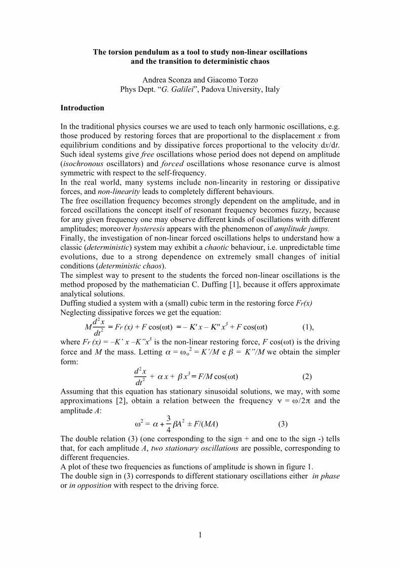
The torsion pendulum as a tool to study non-linear oscillationsand the transition to deterministic chaos

Andrea Sconza and Giacomo TorzoPhys Dept. “G. Galilei”, Padova University, Italy

Introduction

In the traditional physics courses we are used to teach only harmonic oscillations, e.g.those produced by restoring forces that are proportional to the displacement x fromequilibrium conditions and by dissipative forces proportional to the velocity dx/dt.Such ideal systems give free oscillations whose period does not depend on amplitude(isochronous oscillators) and forced oscillations whose resonance curve is almostsymmetric with respect to the self-frequency.In the real world, many systems include non-linearity in restoring or dissipativeforces, and non-linearity leads to completely different behaviours.The free oscillation frequency becomes strongly dependent on the amplitude, and inforced oscillations the concept itself of resonant frequency becomes fuzzy, becausefor any given frequency one may observe different kinds of oscillations with differentamplitudes; moreover hysteresis appears with the phenomenon of amplitude jumps.Finally, the investigation of non-linear forced oscillations helps to understand how aclassic (deterministic) system may exhibit a chaotic behaviour, i.e. unpredictable timeevolutions, due to a strong dependence on extremely small changes of initialconditions (deterministic chaos).The simplest way to present to the students the forced non-linear oscillations is themethod proposed by the mathematician C. Duffing [1], because it offers approximateanalytical solutions.Duffing studied a system with a (small) cubic term in the restoring force Fr(x)Neglecting dissipative forces we get the equation:

Md2xdt2

= Fr (x) + F cos(ωt) = – Κ' x – Κ'' x3 + F cos(ωt) (1),

where Fr (x) = –K’ x –K”x3 is the non-linear restoring force, F cos(ωt) is the drivingforce and M the mass. Letting α = ωo

2 = K’/M e β = K”/M we obtain the simplerform:

d2xdt2

+ α x + β x3 = F/M cos(ωt) (2)

Assuming that this equation has stationary sinusoidal solutions, we may, with someapproximations [2], obtain a relation between the frequency ν = ω /2π and theamplitude A:

ω2 = α +34βA2 ± F/(MA) (3)

The double relation (3) (one corresponding to the sign + and one to the sign -) tellsthat, for each amplitude A, two stationary oscillations are possible, corresponding todifferent frequencies.A plot of these two frequencies as functions of amplitude is shown in figure 1.The double sign in (3) corresponds to different stationary oscillations either in phaseor in opposition with respect to the driving force.

2

Figure 1: Undamped forced oscillations: frequencies vs. amplitude (here α = 0.4 s-2, β = 160 m-2s-2,F/M = 0.044 N/kg)

The two curves in Figure 1 never meet, due to the absence of dissipative term in eq. 1.Introducing a dissipative force proportional to velocity, we obtain the equation:

d2xdt2

+ εdxdt

+ α x + β x3 = F/M cos(ωt) (4),

from which a new approximate relation may be derived in place of previous eq. (3):

(ω2 – α −(3/4)βΑ2 )2 + ω2ε2 = F2/(MA)2 (5).

This is a biquadratic equation in ω , that (neglecting negative roots, physicallymeaningless) gives the plot shown in Figure 2, where the two curves meet at amaximum amplitude beyond which no stable oscillation is possible.

Figure 2: Damped forced oscillations (ε = 0.065 s-1)

The intermediate curve in figure 2 represents the relation between frequency andamplitude for free oscillations, that is obtained from (5) letting F=0 . The departure ofthis curve from the horizontal straight line measures anisochronism of the system.We note that relations (3) and (5), are third order equations in the variable A, andtherefore for each frequency there are up to 3 values of the oscillation amplitude

3

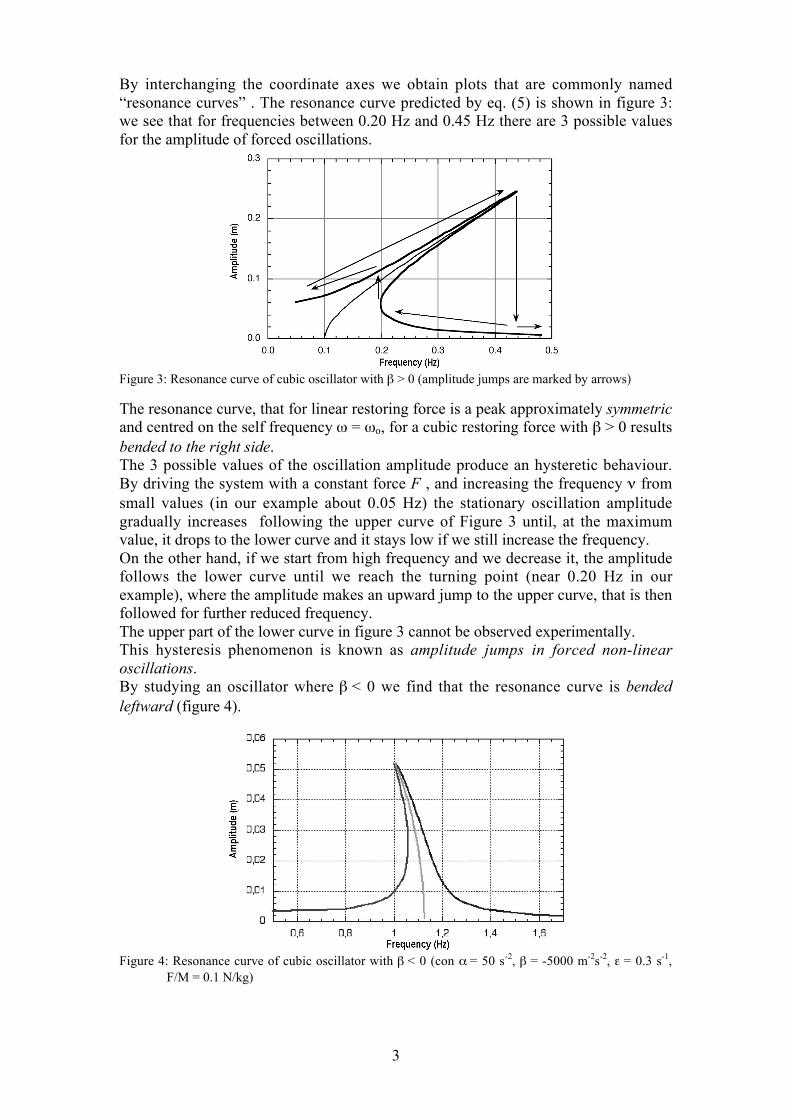
By interchanging the coordinate axes we obtain plots that are commonly named“resonance curves” . The resonance curve predicted by eq. (5) is shown in figure 3:we see that for frequencies between 0.20 Hz and 0.45 Hz there are 3 possible valuesfor the amplitude of forced oscillations.

Figure 3: Resonance curve of cubic oscillator with β > 0 (amplitude jumps are marked by arrows)

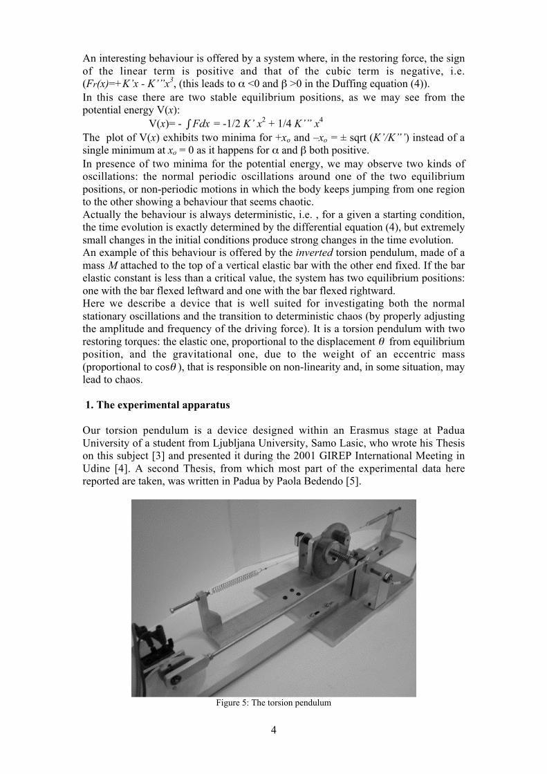
The resonance curve, that for linear restoring force is a peak approximately symmetricand centred on the self frequency ω = ωo, for a cubic restoring force with β > 0 resultsbended to the right side.The 3 possible values of the oscillation amplitude produce an hysteretic behaviour.By driving the system with a constant force F , and increasing the frequency ν fromsmall values (in our example about 0.05 Hz) the stationary oscillation amplitudegradually increases following the upper curve of Figure 3 until, at the maximumvalue, it drops to the lower curve and it stays low if we still increase the frequency.On the other hand, if we start from high frequency and we decrease it, the amplitudefollows the lower curve until we reach the turning point (near 0.20 Hz in ourexample), where the amplitude makes an upward jump to the upper curve, that is thenfollowed for further reduced frequency.The upper part of the lower curve in figure 3 cannot be observed experimentally.This hysteresis phenomenon is known as amplitude jumps in forced non-linearoscillations.By studying an oscillator where β < 0 we find that the resonance curve is bendedleftward (figure 4).

Figure 4: Resonance curve of cubic oscillator with β < 0 (con α = 50 s-2, β = -5000 m-2s-2, ε = 0.3 s-1,F/M = 0.1 N/kg)

4

An interesting behaviour is offered by a system where, in the restoring force, the signof the linear term is positive and that of the cubic term is negative, i.e.(Fr(x)=+K’x - K’”x3, (this leads to α <0 and β >0 in the Duffing equation (4)).In this case there are two stable equilibrium positions, as we may see from thepotential energy V(x):

V(x)= -

€

Fdx∫ = -1/2 K’ x2 + 1/4 K’” x4

The plot of V(x) exhibits two minima for +xo and –xo = ± sqrt (K’/K”’) instead of asingle minimum at xo = 0 as it happens for α and β both positive.In presence of two minima for the potential energy, we may observe two kinds ofoscillations: the normal periodic oscillations around one of the two equilibriumpositions, or non-periodic motions in which the body keeps jumping from one regionto the other showing a behaviour that seems chaotic.Actually the behaviour is always deterministic, i.e. , for a given a starting condition,the time evolution is exactly determined by the differential equation (4), but extremelysmall changes in the initial conditions produce strong changes in the time evolution.An example of this behaviour is offered by the inverted torsion pendulum, made of amass M attached to the top of a vertical elastic bar with the other end fixed. If the barelastic constant is less than a critical value, the system has two equilibrium positions:one with the bar flexed leftward and one with the bar flexed rightward.Here we describe a device that is well suited for investigating both the normalstationary oscillations and the transition to deterministic chaos (by properly adjustingthe amplitude and frequency of the driving force). It is a torsion pendulum with tworestoring torques: the elastic one, proportional to the displacement θ from equilibriumposition, and the gravitational one, due to the weight of an eccentric mass(proportional to cosθ ), that is responsible on non-linearity and, in some situation, maylead to chaos.

1. The experimental apparatus

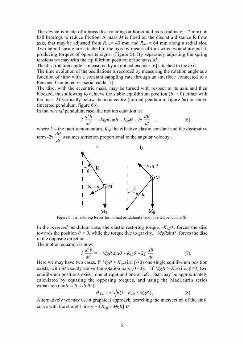
Our torsion pendulum is a device designed within an Erasmus stage at PaduaUniversity of a student from Ljubljana University, Samo Lasic, who wrote his Thesison this subject [3] and presented it during the 2001 GIREP International Meeting inUdine [4]. A second Thesis, from which most part of the experimental data herereported are taken, was written in Padua by Paola Bedendo [5].

Figure 5: The torsion pendulum

5

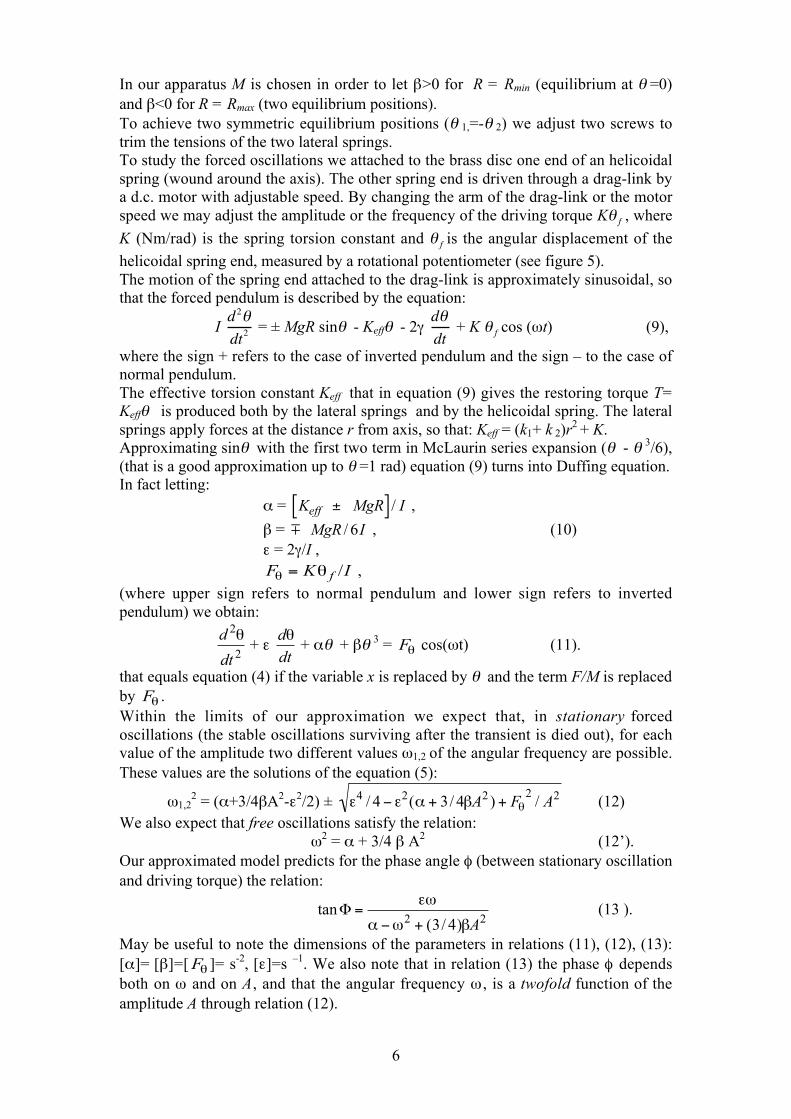
The device is made of a brass disc rotating on horizontal axis (radius r = 7 mm) onball bearings to reduce friction. A mass M is fixed on the disc at a distance R fromaxis, that may be adjusted from Rmin= 43 mm and Rmax= 64 mm along a radial slot.Two lateral spring are attached to the axis by means of thin wires wound around it,producing torques of opposite signs. (Figure 5). By separately adjusting the springtensions we may trim the equilibrium position of the mass M.The disc rotation angle is measured by an optical encoder [6] attached to the axis.The time evolution of the oscillations is recorded by measuring the rotation angle as afunction of time with a constant sampling rate through an interface connected to aPersonal Computed via serial cable [7].The disc, with the eccentric mass, may be turned with respect to its axis and thenblocked, thus allowing to achieve the stable equilibrium position (θ = 0) either withthe mass M vertically below the axis centre (normal pendulum, figure 6a) or above(inverted pendulum, figure 6b).In the normal pendulum case, the motion equation is:

I d2θdt2

= -MgRsinθ - Keffθ - 2γ dθdt

, (6)

where I is the inertia momentum, Keff the effective elastic constant and the dissipative

term -2γ dθdt

assumes a friction proportional to the angular velocity .

Figure 6: the restoring forces for normal pendulum(a) and inverted pendulum (b)

In the inverted pendulum case, the elastic restoring torque, -Keffθ , forces the disctowards the position θ = 0, while the torque due to gravity, +MgRsinθ , forces the discin the opposite directionThe motion equation is now:

I d2θdt2

= + MgR sinθ - Keffθ - 2γ dθdt

(7),

Here we may have two cases. If MgR < Keff (i.e. β>0) one single equilibrium positionexists, with M exactly above the rotation axis (θ =0). If MgR > Keff (i.e. β<0) twoequilibrium positions exist : one at right and one at left , that may be approximatelycalculated by equating the opposing torques, and using the MacLaurin seriesexpansion (sinθ ≈ θ -1/6 θ 3):

θ 1,2 ≈ ±

€

6(1− Keff / MgR ) , (8)

Alternatively we may use a graphical approach, searching the intersection of the sinθcurve with the straight line y =

€

Keff / MgR( ) θ .

6

In our apparatus M is chosen in order to let β>0 for R = Rmin (equilibrium at θ =0)and β<0 for R = Rmax (two equilibrium positions).To achieve two symmetric equilibrium positions (θ 1,=-θ 2) we adjust two screws totrim the tensions of the two lateral springs.To study the forced oscillations we attached to the brass disc one end of an helicoidalspring (wound around the axis). The other spring end is driven through a drag-link bya d.c. motor with adjustable speed. By changing the arm of the drag-link or the motorspeed we may adjust the amplitude or the frequency of the driving torque Kθ f , where

K (Nm/rad) is the spring torsion constant and θ f is the angular displacement of the

helicoidal spring end, measured by a rotational potentiometer (see figure 5).The motion of the spring end attached to the drag-link is approximately sinusoidal, sothat the forced pendulum is described by the equation:

I d2θdt2

= ± MgR sinθ - Keffθ - 2γ dθdt

+ K θ f cos (ωt) (9),

where the sign + refers to the case of inverted pendulum and the sign – to the case ofnormal pendulum.The effective torsion constant Keff that in equation (9) gives the restoring torque T=Keffθ is produced both by the lateral springs and by the helicoidal spring. The lateralsprings apply forces at the distance r from axis, so that: Keff = (k1+ k 2)r

2 + K.Approximating sinθ with the first two term in McLaurin series expansion (θ - θ 3/6),(that is a good approximation up to θ =1 rad) equation (9) turns into Duffing equation.In fact letting:

α =

€

Keff ± MgR[ ] / I ,

β =

€

m MgR / 6I , (10)ε = 2γ/I ,

€

Fθ = Kθ f /I ,

(where upper sign refers to normal pendulum and lower sign refers to invertedpendulum) we obtain:

€

d 2θ

dt 2 + ε

€

dθdt

+ αθ + βθ 3 =

€

Fθ cos(ωt) (11).

that equals equation (4) if the variable x is replaced by θ and the term F/M is replacedby

€

Fθ .Within the limits of our approximation we expect that, in stationary forcedoscillations (the stable oscillations surviving after the transient is died out), for eachvalue of the amplitude two different values ω1,2 of the angular frequency are possible.These values are the solutions of the equation (5):

ω1,22 = (α+3/4βA2-ε2/2) ±

€

ε4 / 4 − ε2(α + 3/ 4βA2 ) + Fθ2

/ A2 (12)We also expect that free oscillations satisfy the relation:

ω2 = α + 3/4 β A2 (12’).Our approximated model predicts for the phase angle φ (between stationary oscillationand driving torque) the relation:

€

tanΦ =εω

α −ω2 + (3/ 4)βA2(13 ).

May be useful to note the dimensions of the parameters in relations (11), (12), (13):[α]= [β]=[

€

Fθ ]= s-2, [ε]=s –1. We also note that in relation (13) the phase φ dependsboth on ω and on A, and that the angular frequency ω , is a twofold function of theamplitude A through relation (12).

7

2. Evaluation of the apparatus parameters

To evaluate the elastic constant k1, k2, we measured the change in length of the lateralsprings under known loads.To evaluate the inertial momentum I we weighted and measured the geometry of allcomponents of the pendulum. The accuracy of this evaluation was checked bycomparing the calculated value of I with the experimental value obtained from themeasurement of the period of free oscillations of the pendulum without eccentric massand without helicoidal spring (compensating the missing mass mslot due to the slot inthe disc with a small added mass that cancels the gravitational restoring torque).Details and results of these measurements are reported hereafter

2.1 Elastic constants k1, k2, K and momentum of inertia I

The calculated momentum of inertia is Icalc =(1.87 ± 0.06) 10-3 kg m2, in goodagreement with the value obtained from the measured period T = (1.49 ± 0.01) s andthe measured values of the elastic constants k1 = (316 ± 9) N/m and k 2 = (313 ± 5)N/m. From relation (2π/T)2 = (k1 + k2)r

2 / I we get in fact I = (1.86±0.09) 10-3 kg m2.With the eccentric mass (M = 107.1 g) placed at Rmin= (43 ± 1) mm we get: Itotal= I +M Rmin

2 = (1.975 ± 0.06) 10-3 kg m2

In the same condition the gravitational torque (accounting for mslot≈ 6 g, and assumingthe missing mass to be concentrated on the mean radius rm=54 mm) is MgR’ = MgRmin

– mslot g rm = (0.042 ± 0.001) Nm.The torsion constant K of the helicoidal spring is indirectly evaluated comparing thefree oscillation periods of the pendulum without any eccentric mass, the one due tothe lateral springs T1 = (1.49 ± 0.01) s and the one due to the axial helicoidal springT2 = 2.12 ± 0.03 s.The ratio between the two torsion constants must equal the square of the inverse ratioof the two periods:

€

K / (k1 + k2 )r 2[ ] = T1 / T2( )2 = 0.493 ± 0.007.

where r is the axis radius (r = 7.25 ± 0.10 mm). This gives K = (1.63 ± 0.06) 10-2

Nm/rad, and Keff = (k1+ k 2)r2 + K = (4.94 ± 0.15) 10-2 Nm/rad.

2.2 The friction coefficient ε

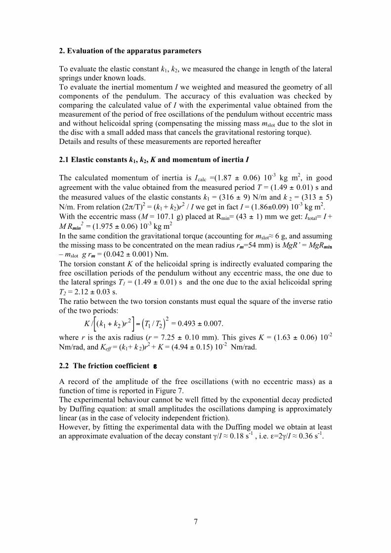
A record of the amplitude of the free oscillations (with no eccentric mass) as afunction of time is reported in Figure 7.The experimental behaviour cannot be well fitted by the exponential decay predictedby Duffing equation: at small amplitudes the oscillations damping is approximatelylinear (as in the case of velocity independent friction).However, by fitting the experimental data with the Duffing model we obtain at leastan approximate evaluation of the decay constant γ/I ≈ 0.18 s-1 , i.e. ε=2γ/I ≈ 0.36 s-1.

8

Figure 7: Free oscillation amplitude as function of time. Dots: experimental results. Line: exponentialbest fit to points at large amplitude.

2.3 Nominal values of the parameters α and β in Duffing equation

Using the calculated values of I, K, k1, k2 in relations (10) we get the nominal valuesfor the parameters α and β of Duffing equation. For R = Rmin, in the two cases ofnormal and inverted pendulum we obtain:αnorm = [K + (k1+k2) r

2 + MgR’] / I = (46.3 ± 1.6) s-2

αinv = [K + (k1+k2) r2 - MgR’] / I = (3.7 ± 1.0) s-2

β norm = - MgR’/(6 I) = - (3.5 ± 0.2) s-2

β inv = + MgR’/(6 I) = + (3.5 ± 0.2) s-2

3. Experimental results and data analysis

We first studied the free damped oscillations whose frequency does strongly dependon the amplitude. Then we investigated the forced oscillations, by keeping the drivingforce at small value in order to be able to observe, after a transient, a stationarymotion with a period identical to that of the driving force (the so-called harmonicoscillations). In this configuration we observed the phenomenon of amplitude jumps,associated to hysteresis.By increasing the driving force we than produced subharmonic oscillations (whoseperiod is longer than that of the driving force). Finally, further increasing theamplitude we observed the transition to chaotic motion.Predictions based on nominal values of the parameters and on approximate equations(12) and (12’) are compared to experimental results for free and forced oscillations,both in the case of normal and of inverted pendulum.One may obviously expect that approximate prediction will match experimentalresults only for small amplitudes.To match experimental data at larger amplitudes we must proceed to numericalintegration of the exact motion equation (4), e.g. using commercial software formodelling as Stella [12].The results of numerical simulations are reported in section 4.

3.1 The normal pendulum

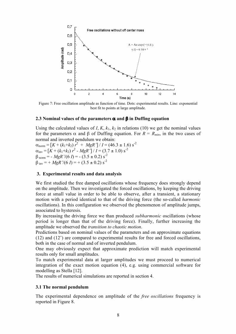
The experimental dependence on amplitude of the free oscillations frequency isreported in Figure 8.

9

The more the oscillation is damped the more its (pseudo)period decreases, followingapproximately the behaviour predicted by relation (12’) with the nominal values of αand β.

Figure 8: the square of the angular frequency as a function of amplitude of the free oscillations ofnormal pendulum (β<0).

The forced oscillations were studied using for the helicoidal spring a drivingamplitude θ f =0.6 rad, by gradually changing the frequency of the driving torque

(either increasing or decreasing it), and always waiting for stabilization of theoscillation amplitude.As shown in figure 9 and 10 (where in the vertical axis we plot the frequency insteadof the square of angular frequency), this procedure leads to hysteresis in the resonancecurve, and to the phenomenon of amplitude jumps.

Figure 9: Experimental relation between frequency and amplitude of forced oscillations in normalpendulum (β<0); increasing frequency () and decreasing frequency (). Dotted line shows thepredicted behaviour of free oscillations.

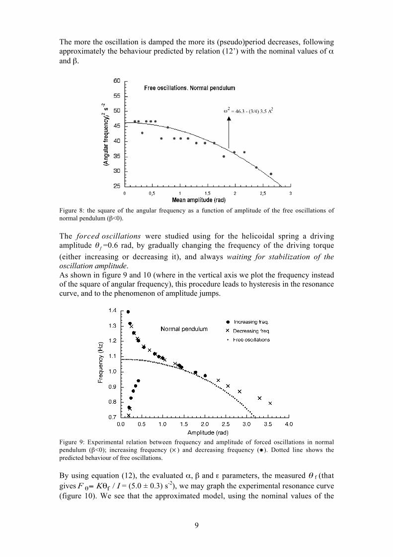
By using equation (12), the evaluated α, β and ε parameters, the measured θ f (thatgives

€

F θ= Kθf / I = (5.0 ± 0.3) s-2), we may graph the experimental resonance curve(figure 10). We see that the approximated model, using the nominal values of the

10

parameters α , β, ε and

€

F θ , is in fair agreement with experimental results up to about2 rad,

Figure 10: comparison of the approximated theory with experimental data for normal pendulum (β<0)

We also measured the phase angle Φ between the driving torque and the stationaryoscillation as a function of frequency (figure 11).Because in equation (13) Φ depends both on amplitude and frequency, to calculate thecurve shown in figure 11 we first calculate for each amplitude the corresponding twovalues of frequency through equation (12) and then we insert them into (13) to obtainΦ1,2.

Figure 11: Phase angle measured increasing () and decreasing () frequency, compared with thevalues Φ1,2 calculated from approximated theory

We observe that the phase angle is nearly zero at the lower frequencies (oscillations inphase with the driving torque) and nearly π at the higher frequencies (oscillations inopposition with the driving torque).

3.2 Inverted pendulum

In the case of inverted pendulum, the free oscillations damp much faster than in thecase of normal pendulum because the restoring torque is now the difference (and not

11

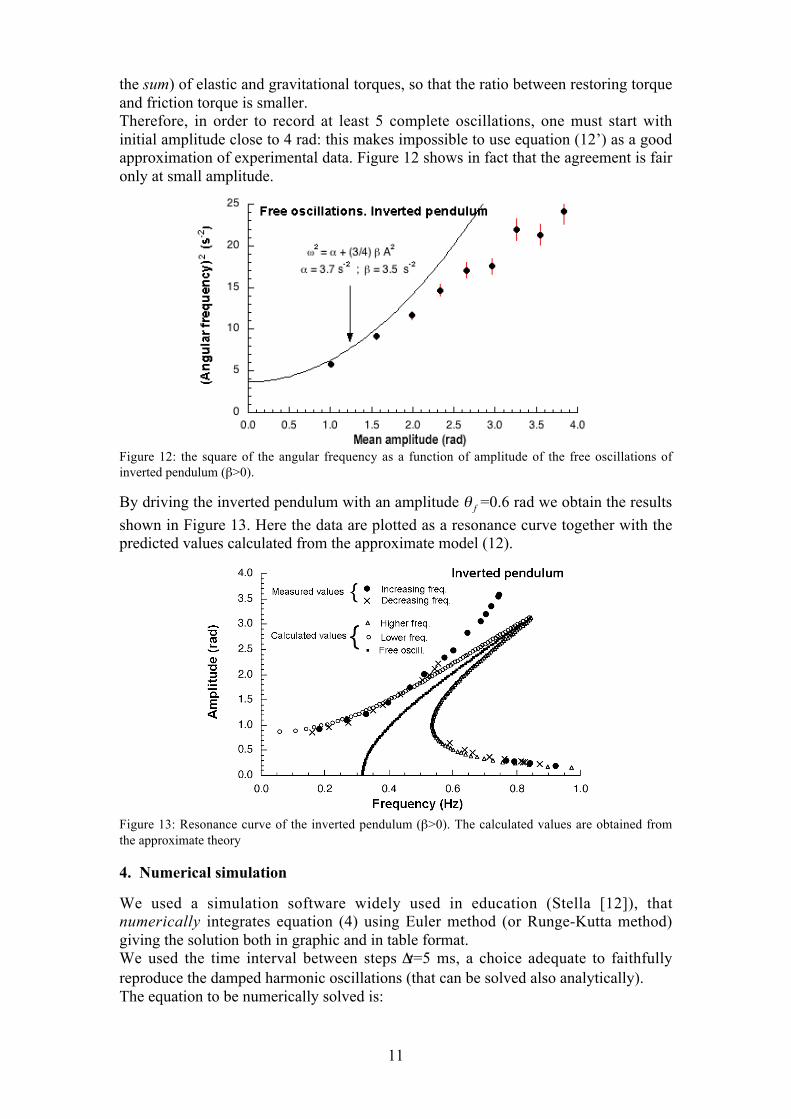
the sum) of elastic and gravitational torques, so that the ratio between restoring torqueand friction torque is smaller.Therefore, in order to record at least 5 complete oscillations, one must start withinitial amplitude close to 4 rad: this makes impossible to use equation (12’) as a goodapproximation of experimental data. Figure 12 shows in fact that the agreement is faironly at small amplitude.

Figure 12: the square of the angular frequency as a function of amplitude of the free oscillations ofinverted pendulum (β>0).

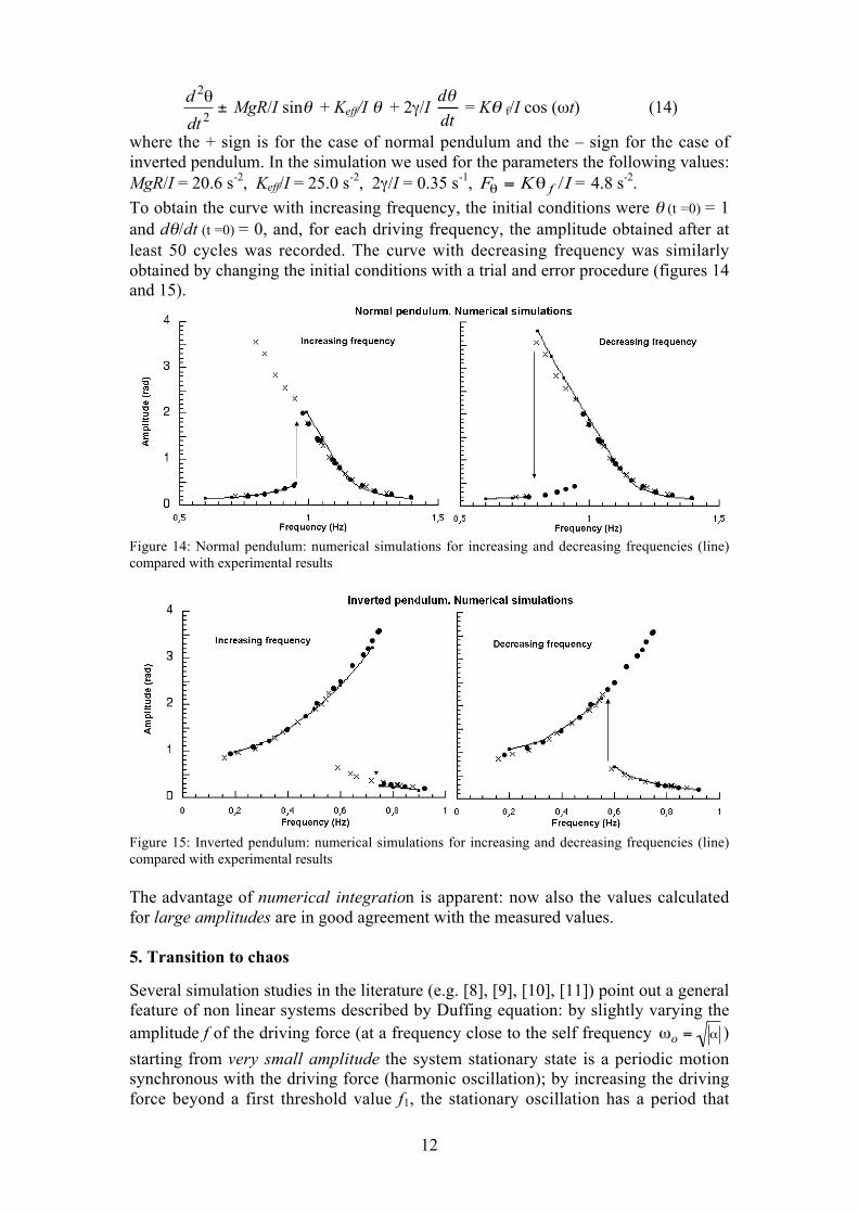
By driving the inverted pendulum with an amplitude θ f =0.6 rad we obtain the results

shown in Figure 13. Here the data are plotted as a resonance curve together with thepredicted values calculated from the approximate model (12).

Figure 13: Resonance curve of the inverted pendulum (β>0). The calculated values are obtained fromthe approximate theory

4. Numerical simulation

We used a simulation software widely used in education (Stella [12]), thatnumerically integrates equation (4) using Euler method (or Runge-Kutta method)giving the solution both in graphic and in table format.We used the time interval between steps Δt=5 ms, a choice adequate to faithfullyreproduce the damped harmonic oscillations (that can be solved also analytically).The equation to be numerically solved is:

12

€

d 2θ

dt 2± MgR/I sinθ + Keff/I θ + 2γ/I

dθdt

= Kθ f/I cos (ωt) (14)

where the + sign is for the case of normal pendulum and the – sign for the case ofinverted pendulum. In the simulation we used for the parameters the following values:MgR/I = 20.6 s-2, Keff/I = 25.0 s-2, 2γ/I = 0.35 s-1,

€

Fθ = Kθ f /I = 4.8 s-2.

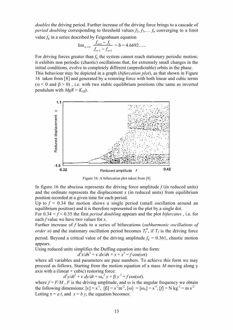
To obtain the curve with increasing frequency, the initial conditions were θ (t =0) = 1and dθ/dt (t =0) = 0, and, for each driving frequency, the amplitude obtained after atleast 50 cycles was recorded. The curve with decreasing frequency was similarlyobtained by changing the initial conditions with a trial and error procedure (figures 14and 15).

Figure 14: Normal pendulum: numerical simulations for increasing and decreasing frequencies (line)compared with experimental results

Figure 15: Inverted pendulum: numerical simulations for increasing and decreasing frequencies (line)compared with experimental results

The advantage of numerical integration is apparent: now also the values calculatedfor large amplitudes are in good agreement with the measured values.

5. Transition to chaos

Several simulation studies in the literature (e.g. [8], [9], [10], [11]) point out a generalfeature of non linear systems described by Duffing equation: by slightly varying theamplitude f of the driving force (at a frequency close to the self frequency

€

ωo = α )

starting from very small amplitude the system stationary state is a periodic motionsynchronous with the driving force (harmonic oscillation); by increasing the drivingforce beyond a first threshold value f1, the stationary oscillation has a period that

13

doubles the driving period. Further increase of the driving force brings to a cascade ofperiod doubling corresponding to threshold values f2, f3,… fn converging to a limit

value fc in a series described by Feigenbaum equation

limn→∞ fn+1 − fnfn+ 2 − fn+1

= δ = 4.6692…..

For driving forces greater than fc the system cannot reach stationary periodic motion;it exhibits non periodic (chaotic) oscillations that, for extremely small changes in theinitial conditions, evolve in completely different (unpredictable) orbits in the phase.This behaviour may be depicted in a graph (bifurcation plot), as that shown in Figure16 taken from [8] and generated by a restoring force with both linear and cubic terms(α < 0 and β > 0) , i.e. with two stable equilibrium positions (the same as invertedpendulum with MgR > Keff).

Figure 16: A bifurcation plot taken from [8]

In figure 16 the abscissa represents the driving force amplitude f (in reduced units)and the ordinate represents the displacement x (in reduced units) from equilibriumposition recorded at a given time for each period.Up to f = 0.34 the motion shows a single period (small oscillation around anequilibrium position) and it is therefore represented in the plot by a single dot.For 0.34 < f < 0.35 the first period doubling appears and the plot bifurcates , i.e. foreach f value we have two values for x.Further increase of f leads to a series of bifurcations (subharmonic oscillations oforder n) and the stationary oscillation period becomes Tf

n, if Tf is the driving force

period. Beyond a critical value of the driving amplitude fc = 0.361, chaotic motionappears.Using reduced units simplifies the Duffing equation into the form:

d2x/dτ2 + ε dx/dτ + x + x3 = f cos(ωτ)where all variables and parameters are pure numbers. To achieve this form we mayproceed as follows. Starting from the motion equation of a mass M moving along yaxis with a (linear + cubic) restoring force:

d2y/dt2 + ε dy/dt + ωo2 y + β y 3 = f cos(ωt).

where f = F/M , F is the driving amplitude, and ω is the angular frequency we obtainthe following dimensions: [ε] = s-1, [β] = s-2m-2, [ω] = [ωo] = s-1, [f] = N kg-1 = m s-2

Letting τ = a t, and x = b y, the equation becomes:

14

(a2/b) d2x/dτ2 + ε (a/b) dx/dτ + (ωo2/b) x + (β/b3) x3 = f cos (ωτ/a).

Multiplying by b/a2 we getd2x/dτ2 + ε/a dx/dτ + (ωo

2/a2) x + β/(a2b2) x3 = f b/a2 cos (ωτ/a).By choosing a = ωo

and b2 = β /a2 = β /ωo2

And using the reduced variables x, τ , ε’, ω’ and f ’:ε’ = ε / ωo, f ’ = f β1/2 / ωo

3

ω’ = ω / ωo (14)τ = ωo

t x = (β1/2 / ωo) y.the equation becomes

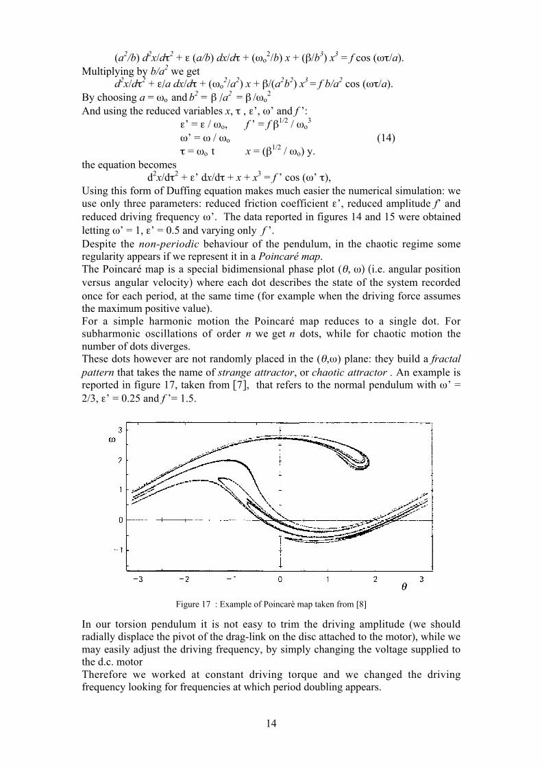
d2x/dτ2 + ε’ dx/dτ + x + x3 = f ’ cos (ω’ τ),Using this form of Duffing equation makes much easier the numerical simulation: weuse only three parameters: reduced friction coefficient ε’, reduced amplitude f’ andreduced driving frequency ω’. The data reported in figures 14 and 15 were obtainedletting ω’ = 1, ε’ = 0.5 and varying only f ’.Despite the non-periodic behaviour of the pendulum, in the chaotic regime someregularity appears if we represent it in a Poincaré map.The Poincaré map is a special bidimensional phase plot (θ, ω) ( i.e. angular positionversus angular velocity) where each dot describes the state of the system recordedonce for each period, at the same time (for example when the driving force assumesthe maximum positive value).For a simple harmonic motion the Poincaré map reduces to a single dot. Forsubharmonic oscillations of order n we get n dots, while for chaotic motion thenumber of dots diverges.These dots however are not randomly placed in the (θ,ω) plane: they build a fractalpattern that takes the name of strange attractor, or chaotic attractor . An example isreported in figure 17, taken from [7], that refers to the normal pendulum with ω’ =2/3, ε’ = 0.25 and f ’= 1.5.

Figure 17 : Example of Poincarè map taken from [8]

In our torsion pendulum it is not easy to trim the driving amplitude (we shouldradially displace the pivot of the drag-link on the disc attached to the motor), while wemay easily adjust the driving frequency, by simply changing the voltage supplied tothe d.c. motorTherefore we worked at constant driving torque and we changed the drivingfrequency looking for frequencies at which period doubling appears.

15

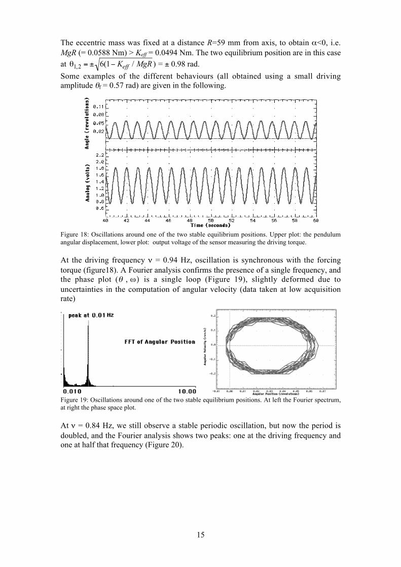
The eccentric mass was fixed at a distance R=59 mm from axis, to obtain α<0, i.e.MgR (= 0.0588 Nm) > Keff = 0.0494 Nm. The two equilibrium position are in this caseat

€

θ1,2 = ± 6(1− Keff / MgR ) = ± 0.98 rad.

Some examples of the different behaviours (all obtained using a small drivingamplitude θf = 0.57 rad) are given in the following.

Figure 18: Oscillations around one of the two stable equilibrium positions. Upper plot: the pendulumangular displacement, lower plot: output voltage of the sensor measuring the driving torque.

At the driving frequency ν = 0.94 Hz, oscillation is synchronous with the forcingtorque (figure18). A Fourier analysis confirms the presence of a single frequency, andthe phase plot (θ , ω) is a single loop (Figure 19), slightly deformed due touncertainties in the computation of angular velocity (data taken at low acquisitionrate)

Figure 19: Oscillations around one of the two stable equilibrium positions. At left the Fourier spectrum,at right the phase space plot.

At ν = 0.84 Hz, we still observe a stable periodic oscillation, but now the period isdoubled, and the Fourier analysis shows two peaks: one at the driving frequency andone at half that frequency (Figure 20).

16

Figure 20: Period doubling. At left the time evolution, at right the Fourier spectrum: two peaks at 0.84Hz and 0.415 Hz

The phase space plot shows two intersecting loops and the numerical simulation withStella does well reproduce the experimental pattern (Figure 21),

Figure 21: Period doubling in the phase space plot. At left the experimental data , at right the numericalsimulation.

At ν = 0.76 Hz, we observe oscillations with a period that is four times the drivingperiod ( Figure 22)

Figure 22: Second period doubling. At left the time evolution, at right the Fourier spectrum: three peaksat 0.186, 0.391 and 0.771 Hz

The Fourier spectrum shows indeed peaks at 1/2 and 1/4 of the driving frequency, andthe Stella simulation gives a plot in phase space similar to the experimental one(Figure 23)

17

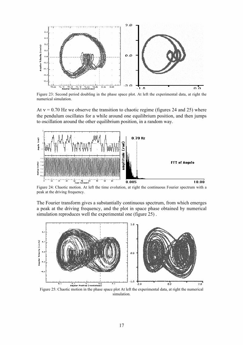
Figure 23: Second period doubling in the phase space plot. At left the experimental data, at right thenumerical simulation.

At ν = 0.70 Hz we observe the transition to chaotic regime (figures 24 and 25) wherethe pendulum oscillates for a while around one equilibrium position, and then jumpsto oscillation around the other equilibrium position, in a random way.

Figure 24: Chaotic motion. At left the time evolution, at right the continuous Fourier spectrum with apeak at the driving frequency.

The Fourier transform gives a substantially continuous spectrum, from which emergesa peak at the driving frequency, and the plot in space phase obtained by numericalsimulation reproduces well the experimental one (figure 25) .

Figure 25: Chaotic motion in the phase space plot At left the experimental data, at right the numericalsimulation.

18

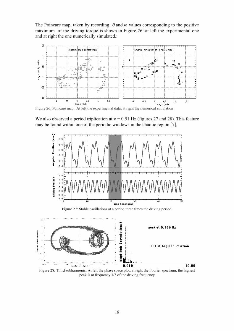
The Poincaré map, taken by recording θ and ω values corresponding to the positivemaximum of the driving torque is shown in Figure 26: at left the experimental oneand at right the one numerically simulated.:

Figure 26: Poincaré map . At left the experimental data, at right the numerical simulation

We also observed a period triplication at ν = 0.51 Hz (figures 27 and 28). This featuremay be found within one of the periodic windows in the chaotic region [7],

Figure 27: Stable oscillations at a period three times the driving period.

Figure 28: Third subharmonic. At left the phase space plot, at right the Fourier spectrum: the highestpeak is at frequency 1/3 of the driving frequency

19

6. “Historical” remarks, acknowledgements and a bibliographic list

The idea of this didactical apparatus was born during a discussion of one of theauthors (G.T.) with prof. Arturo Loria after the 30th International Physics Olympiadheld in Padua in 1999, about the problem on inverted torsion pendulum assigned tothe students as part of the experimental competition. The very simple device given tothe students was cleverly designed by Edoardo Miletti [13] in order to allow eitherhorizontal or vertical rotation axis, and the torque of the eccentric mass could beadjusted by screwing or unscrewing the threaded pendulum rod, thus allowing to varythe system behaviour and showing bifurcation.Prof. Loria (who was aware of the various computer-assisted experiments previouslydesigned by the authors for didactic laboratory) suggested us to setup an apparatusthat could make possible both real time data acquisition of the system evolution andcontrolled forced oscillations, in order to exploit the full range of educational use ofthis interesting device.Our first step was to prepare a prototype on which Samo Lasic’s thesis was based,demonstrating essentially all the features described in the present paper. Thenumerical simulations, as well as a more complete analysis of the system, wereperformed within the thesis later assigned to Paola Bedendo.The result is an experiment that, using simple and cheap tools, allows to fullyinvestigate both linear and non-linear oscillators with a complete control of all theinteresting parameters.Both approximate-analytical and exact-numerical solutions of the Duffing oscillatormay be tested in comparison with experimental measurement, leading to a deeperunderstanding of complex phenomena.In order to make easier to the reader a comparison of our apparatus with similarsystems described in the literature, we add hereafter a list of references on this topic,in chronological order.

T. W. Arnold, W. Case, Nonlinear effects in a simple mechanical system, Am. J.Phys. 50 (1982)

K. Luchner, Chaotic motion: Mechanical systems in experiment and simulation, Bildder Wissenschaft 4 (1983)

H. J. Janssen, R. Serneels, L. Beerden, E. L. M. Flerackers, Experimentaldemonstration of the resonance effect of an anharmonic oscillator, Am. J. Phys. 51(1983)

K. Briggs, Simple experiments in chaotic dynamics, Am. J. Phys. 55 (1987)B. Duchesne, C. W. Fischer, C. G. Gray, K. R. Jeffrey, Chaos in the motion of an

inverted pendulum: An undergraduate laboratory experiment, Am. J. Phys. 59(1991)

N. Alessi, C. W. Fischer, C. G. Gray, Measurement of amplitude jumps andhysteresis in a driven inverted pendulum, Am. J. Phys. 60 (1992)

R. Cuerno, A. F. Ranjada, J. J. Ruiz-Lorenzo, Deterministic chaos in the elasticpendulum: A simple laboratory for nonlinear dynamics, Am. J. Phys. 60 (1992)

K. Weltner, A. S. C. Esperidiao, R. F. S. Andrade, G. P. Guedes, Demonstratingdifferent forms of the bent tuning curve with a mechanical oscillator, Am. J. Phys.62 (1994)

R. D. Peters, Chaotic pendulum based on torsion and gravity in opposition, Am. J.Phys., 63 (1995)

A. Siahmakoun, V. A. French, J. Patterson, Nonlinear dynamics of a sinusoidallydriven pendulum in a repulsive magnetic field, Am. J. Phys. 65 (1997)

20

A. Prosperetti, Subharmonics and ultraharmonics in the forced oscillations of weaklynonlinear systems, Am. J. Phys. 44 (1997)

B. K. Jones, G. Trefan, The Duffing oscillator: A precise electronic analog chaosdemonstrator for the undergraduate laboratory, Am. J. Phys., 69 (2001)

References[1] G. Duffing Erzwungene Schwingungen bei veränderlicher Eigenfrequenz,

F.Wieweg u. Sohn, Braunschweig (1918)[2] J.J. Stoker: Nonlinear vibrations in Mechanical and Electrical Systems,

Interscience Publishers (1950)[3] S. Lasic: Didactical treatment of torsion pendulum with the transition to chaos ,

Thesis, University of Ljubljana, Faculty for Mathematics and Physics, 2001[4] S. Lasic , G. Planinsic, G.Torzo : Torsion pendulum: a mechanical nonlinear

oscillator, Proceedings GIREP 2001, Udine (2001)[5] P. Bedendo: Oscillatori lineari e non-lineari e fenomeni caotici, Tesi di laurea ,

Padova, 2002[6] Home-made sensor equivalent to Rotary Sensors produced by MAD

(http://www.edumad.com), PASCO (http://www.pasco.com), Vernier Software(http://www.vernier.com) and LABTREK (http://www.labtrek.net)

[7] We used the ULI interface from Vernier (http://www.vernier.com), with softwareRotaryMotion for Macintosh. Identical results may be obtained with similarinterfaces (e.g. Vernier-LabPro, Pasco-CI500)

[8] G. L. Baker and J. P. Gollub: Chaotic Dynamics, an introduction, CambridgeUniversity Press, 1990

[9] M. Lakshmanan e K. Murali: Chaos in Nonlinear Oscillators World Scientific1996, Cap 4

[10] M. Lakshmanan e K. Murali: Physics News 24, 3 (1993)[11] C. L. Olson, M. G. Olsson, Dynamical symmetry breaking and chaos in

Duffing’s equation, Am. J. Phys. 59 (1991)[12] Stella Research, vers. 5.1, software distributed by High Performance Systems

Inc., http://www.hps-inc.com[13] E. Milotti: Non linear behaviour in a torsion pendulum, Eur. J. Phys. 22 (2001)