The Time–Money Trade-Off for Entrepreneurs: When to Hire

University of Pennsylvania University of Pennsylvania

ScholarlyCommons ScholarlyCommons

Finance Papers Wharton Faculty Research

2016

The Time–Money Trade-Off for Entrepreneurs: When to Hire the The Time–Money Trade-Off for Entrepreneurs: When to Hire the

First Employee? First Employee?

Onesun Steve Yoo

Guillaume Roels

Charles J. Corbett

Follow this and additional works at: https://repository.upenn.edu/fnce_papers

Part of the Finance and Financial Management Commons

Recommended Citation Recommended Citation Yoo, O. S., Roels, G., & Corbett, C. J. (2016). The Time–Money Trade-Off for Entrepreneurs: When to Hire the First Employee?. Manufacturing & Service Operations Management, 18 (4), 559-569. http://dx.doi.org/10.1287/msom.2016.0587

This paper is posted at ScholarlyCommons. https://repository.upenn.edu/fnce_papers/138 For more information, please contact [email protected].

https://repository.upenn.edu/

https://repository.upenn.edu/fnce_papers

https://repository.upenn.edu/wharton_faculty

https://repository.upenn.edu/fnce_papers?utm_source=repository.upenn.edu%2Ffnce_papers%2F138&utm_medium=PDF&utm_campaign=PDFCoverPages

http://network.bepress.com/hgg/discipline/631?utm_source=repository.upenn.edu%2Ffnce_papers%2F138&utm_medium=PDF&utm_campaign=PDFCoverPages

http://dx.doi.org/10.1287/msom.2016.0587

http://dx.doi.org/10.1287/msom.2016.0587

https://repository.upenn.edu/fnce_papers/138

mailto:[email protected]

The Time–Money Trade-Off for Entrepreneurs: When to Hire the First Employee? The Time–Money Trade-Off for Entrepreneurs: When to Hire the First Employee?

Abstract Abstract For many early-stage entrepreneurs, hiring the first employee is a critical step in the firm’s growth. Doing so often requires significant time and monetary investments. To understand the trade-offs involved in deciding when to hire the first employee and how hiring differs in entrepreneurial settings from more established firm settings, we present a simple growth model that depends on two critical inputs for revenue generation: the entrepreneur’s time and money. We show that without hiring, the entrepreneur’s time eventually becomes more valuable than money in contributing to the firm’s growth. In that context, the value of the employee is driven by how much relief he provides to the entrepreneur. We characterize the optimal timing of hiring in terms of the firm’s cash position and how the firm is affected if it requires an upfront fixed investment in time and/or money. We find that the upfront investment in time needed for hiring cannot be converted to an equivalent upfront investment in money and that mistiming hiring can be very costly, especially when these upfront investments are high.

Keywords Keywords entrepreneurial operations, hiring, optimal stopping problem

Disciplines Disciplines Business | Finance and Financial Management

This journal article is available at ScholarlyCommons: https://repository.upenn.edu/fnce_papers/138

https://repository.upenn.edu/fnce_papers/138

Submitted tomanuscript (Please, provide the mansucript number!)

The Time-Money Trade-Off for Entrepreneurs:When to Hire the First Employee?

Onesun Steve YooDepartment of Management Science and Innovation, University College London,

London WC1E 6BT, United Kingdom, [email protected]

Guillaume RoelsUCLA Anderson School of Management, 110 Westwood Plaza, Los Angeles, CA 90095, USA,

[email protected]

Charles J. CorbettUCLA Anderson School of Management, 110 Westwood Plaza, Los Angeles, CA 90095, USA,

[email protected]

Entrepreneurs need to invest money and time to grow their firms. Both money and time are often scarce, but

the nature of these two resources is fundamentally different. Considering a small, fast-growing entrepreneurial

firm, we show that the firm’s key bottleneck resource shifts from money to time as the firm grows, and

we characterize hiring as an operational mechanism for trading money for time to accelerate growth. The

optimal time for entrepreneurs to hire their first employee occurs as soon as their available cash is sufficiently

large, in order to alleviate the time bottleneck. We show that the cash threshold determined from a one-step

look-ahead policy is optimal when growth is deterministic and performs well even when that is not the case.

We find that hiring costs delay hiring, whereas hiring times may either delay or expedite hiring, because of

the non-trivial tradeoff between the need to preserve the growth momentum and the need to hire before the

opportunity cost of time becomes too large. Hence, time and money should be managed as distinct resources

in growth-oriented firms.

Key words : Entrepreneurial Operations, Capacity Investment, Hiring, Bottleneck, Dynamic Programming,

Supermodularity, Heuristic.

“There are only three fundamental resources you will be working with to achieve your

entrepreneurial goals: time, people, and money. As an entrepreneur, you can usually trade one

for the others.” (Burgstone and Murphy 2012, Breakthrough Entrepreneurship, p. 156)

1. Introduction

For many entrepreneurs presented with a growth opportunity, realizing that growth is not without

challenges. The firm often lacks the necessary resources and faces a realistic possibility of imminent

failure (Hamermesh et al. 2005). Scaling the business and capitalizing on the growth opportunity

during this phase strongly depends on the entrepreneur’s ability to manage the firm’s limited

resources.

1

Author: The Time-Money Trade-Off for Entrepreneurs2 Article submitted to ; manuscript no. (Please, provide the mansucript number!)

Among the scarce resources, two particularly fundamental ones are money and time. A phase of

high growth puts severe pressure on the entrepreneur’s financial resources (Hambrick and Crozier

1985) and many entrepreneurs are unable to scale their business due to funding difficulties (Evans

and Jovanovic 1989). To fund their growth, many firms reinvest their earnings (Ebben and Johnson

2006) and often borrow the necessary funds (Berger and Udell 1998). At the same time, as the firm

expands, an increasing number of tasks require the entrepreneur’s attention, now putting pressure

on her time and processing capacity (Gifford 1992). Some activities cannot be easily delegated, so

entrepreneurs often find themselves becoming the bottleneck resource of their firms (Martin and

Papadimitriou 2009). When the entrepreneur’s time is the bottleneck, hiring can be viewed as a

way to alleviate that constraint so as to sustain the firm’s growth, as illustrated by the following

quote: “Typically, when a company is founded by a group of motivated and bright individuals, the

founding team is involved in most aspects of the company’s operations in the early days . . . as the

company grows, it must hire new employees, because the founding team is capacity constrained and

does not have the bandwidth to be involved in all aspects of the company operations” (Krishnan

2013, p. 3).

While time and money are both necessary resources for growth, they are inherently different. In

this paper we explore how entrepreneurs can trade time and money, and explore the consequences

of the inherent asymmetry between the two. First, money, unlike time, is fungible. Whereas money

can be accumulated (or borrowed) across periods, time is only available in a limited budget each

period (e.g., 30 days per month) and is perishable. Although activities can be shifted between

periods, leftover time cannot be stored nor can extra time be created. Second, the result of the

firm’s core activity is money, not time. The output of the firm in one period can be reinvested into

the firm in the form of money in the next period but not in the form of time. To better manage the

two resources, one must first understand the implications of these properties of time and money.

How does the severity of the time and money constraints evolve during the growth phase? To

address this question, we introduce a finite-horizon growth model for entrepreneurial firms in which

revenue in each period is a function of two complementary inputs: money and time. The constraint

on time represents the amount of time that exists each period (e.g., 30 days per month), and the

constraint on money represents the amount of money available in the firm (initial starting capital

and accumulated revenue). We examine the evolution of the shadow prices of time and money

and show that the bottleneck always shifts from money to time, meaning that time will eventually

become more valuable than money as the firm grows, an immediate consequence of the asymmetry

between the two. We introduce hiring as a mechanism to alleviate the time bottleneck (Goldratt

2004), trading off money (wages) for additional time (via delegation) to allow faster growth.

Author: The Time-Money Trade-Off for EntrepreneursArticle submitted to ; manuscript no. (Please, provide the mansucript number!) 3

When should entrepreneurs hire their first employee? Hiring too early or too late can inhibit

growth: “Too often, those who bring the business to the success stage are unsuccessful... either

because they try to grow too fast and run out of cash..., or are unable to delegate effectively enough

to make the company work” (Churchill and Lewis 1983, p. 9). In our context, hiring an employee

represents an agreement to trade off a fixed amount of money for a fixed amount of time each

period for the remainder of the horizon. Moreover, hiring (and training) often entails fixed costs of

money and time, referred to as hiring cost and hiring time, which temporarily slows down the firm’s

growth (Tansky and Heneman 2006, Aldrich and Fiol 1994, Collins and Clark 2003, Williamson

2000). Furthermore, hiring may increase the probability of bankruptcy. In such a setting, with

growth and uncertainty, there is limited guidance on when an entrepreneur should hire.

We define the timing of hiring in terms of a cash threshold defined by the one-stage-look-ahead

(OSLA) rule. We show that this policy is optimal when growth is deterministic and numerically

performs well when that is not the case (Babich and Sobel 2004). The high performance of the

OSLA policy is robust to the problem parameters in our growth setting.

Focusing on the OSLA hiring policy, we examine how various factors influence the timing of

hiring. We find that hiring is delayed when hiring costs are higher. However, greater hiring time

can either expedite or delay hiring, because of two conflicting effects. On the one hand, increased

hiring time diverts more valuable time away from growth activities, which slows growth, pushing

for later hiring. On the other hand, it may be more desirable to incur a larger hiring time when

time is less valuable, pushing for earlier hiring. Hence, time and money should be considered as

distinct resources in growth-oriented firms. We replicate the analysis to investigate the optimal

timing of firing and show that the insights mirror those for hiring. We numerically examine hiring

with and without firing, and find that the option of firing does not materially influence the timing

of hiring.

This paper is organized as follows. We review related literature in §2. In §3, we introduce the

growth model and characterize the shift in bottleneck from money to time. In §4, we present the

hiring model, characterize the OSLA hiring and firing policies separately, study their sensitivity,

and demonstrate their optimality under certain conditions. We show numerically in §5 that the

OSLA policy performs well in general, and we conclude in §6. All proofs appear in the appendix.

2. Related Literature

We draw on three strands of literature: that on entrepreneurship and growth, the emerging litera-

ture on entrepreneurial operations, and that on capacity expansion.


2.1. Bottlenecks in Growth-Oriented Entrepreneurial Firms

Firms typically go through several distinct phases in their life cycles from being a start-up to an

established firm, each with its own specific objectives and constraints (Quinn and Cameron 1983).

Typically, entrepreneurial firms initially face considerable uncertainty, and their goal is to learn

and to innovate a viable product while acquiring necessary funding to survive (Jovanovic 1982).

However, once they have learned about their market, true costs, and relative efficiency, the firms’

primary concern becomes centered around growth (Quinn and Cameron 1983).

Maximizing growth during this phase strongly depends on the entrepreneur’s ability to manage

the firm’s limited resources. Some authors identify cash as being the main constraining factor for

growth (e.g., Hambrick and Crozier 1985, Evans and Jovanovic 1989, Ebben and Johnson 2006),

whereas others identify the entrepreneur herself as the main bottleneck (Cressy 1996, Martin and

Papadimitriou 2009), given that growth creates additional demands for the entrepreneur’s attention

and time (Gifford 1992). In line with the latter school of thought, how entrepreneurs allocate their

time has received recent interest from the entrepreneurship literature (Levesque and Schade 2005,

Mueller et al. 2012). In the same spirit, Yoo et al. (2011) examine how they should allocate their

time between process improvement and revenue growth.

In this paper, we unify the money-focused and time-focused viewpoints by demonstrating that

both time and money are bottlenecks, but at different stages of the firm’s growth. Considering

a similar trade-off, Levesque and MacCrimmon (1997) investigate how much time entrepreneurs

should allocate to the venture initiation when they have regular hourly wage jobs. Similar to our

model, time and money are assumed to be complementary. In their model, it is the wage job

opportunity, and not hiring, that substitutes time for money. In contrast, we focus here on venture

growth, and not initiation, and consider hiring as a one-time, irreversible decision to increase time;

accordingly, properly timing hiring is key to achieve successful growth.

2.2. Entrepreneurial Operations and Finance

Many entrepreneurial firms face high uncertainty and lack financial resources, resulting in a high

probability of failure. A growing body of operations management literature on entrepreneurial firms

addresses these key issues.

2.2.1. Reducing Bankruptcy Probability. Some studies examine how operational deci-

sions can minimize the likelihood of bankruptcy. When the firm’s objective is to maximize survival

probability, Archibald et al. (2002) show that inventory decisions should be more conservative and

Swinney et al. (2011) examine a start-up’s timing of capacity investments when competing against

established firms. Tanrisever et al. (2012) examine the decision to invest in process improvement

under the threat of bankruptcy. Unlike some of these works in which avoiding bankruptcy is the


objective, we consider bankruptcy as a terminating condition, and our objective is growth, similar

to maximizing the expected value of payoff in IPO (Babich and Sobel 2004).

2.2.2. Relaxing Financial Constraints. Many studies address the financing challenges

faced by startups and fast growing companies. Buzacott and Zhang (2004) examine how asset-based

financing can be used to manage their operations. Li et al. (2009) acknowledge the considerable

interaction between the operations policy and the financing decisions for cash-constrained small

growing firms and examine the impact of coordinating them. They find that the production and

borrowing policy that maximizes the long-term value of dividends while avoiding bankruptcy is

myopic. We obtain a similar result with the objective of maximizing the firm’s long-term cash

position. Sobel and Turcic (2007) examine how to use credit to better manage resources in nascent

firms and show that the benefit from coordinating finance and operations is greater for smaller

firms. Xu and Birge (2006) show that operational and financial decisions must be made jointly when

capital markets are imperfect, i.e., in the presence of taxes and bankruptcy costs, and Dada and

Hu (2008) and Kouvelis and Zhao (2011) further extend this by considering strategic interactions

between the bank and the firm, and for the latter, a supplier.

We contribute to the literature on financing operations in two ways. First, we consider a non-

fungible resource, namely time, as a potential bottleneck in addition to money. In contrast, most

of the literature on financing operations focuses on the interplay between two substitutable and

fungible resources (e.g., cash and inventory). Second, given that the time span of hiring decisions

is typically longer than that of inventory decisions (Holt et al. 1960) we adopt a more tactical

perspective on the operations of entrepreneurial firms.

2.3. Capacity Expansion and Production Planning

Hiring (and delegating tasks) in small firms increases the available time for the entrepreneur,

enhancing the firm’s capacity to grow. According to Dixit and Pindyck (1994), capacity decisions

share three important characteristics: (i) investments are partially or completely irreversible, (ii)

there exists uncertainty over future rewards, and (iii) there is leeway in the timing of investment.

Our decision of when to hire a permanent employee under uncertainty in future rewards shares

all three characteristics, so it relates to the extensive operations literature on capacity expansion

(Luss 1982, Van Mieghem 2003). This literature typically considers a large firm in which exogenous

demand is assumed to increase, either deterministically (Manne 1961) or stochastically (Luss 1982).

We contribute to this literature by presenting a different type of capacity expansion for growing

firms. First, we allow capacity expansion to cost both time and money, unlike traditional models

in which the expansion cost is purely monetary (Ye and Duenyas 2007). We show that hiring times


and hiring costs have different effects on the timing of hiring: in the small growing firm setting,

time and money must not be aggregated as is often implicitly done for established firms.

Second, we demonstrate a fundamental bottleneck shift between time (capacity) and money as

the firm grows. Most of the literature on capacity expansion focuses only on capacity as a potential

bottleneck, with a few exceptions that consider both capacity and money. Angelus and Porteus

(2002) characterize the optimal capacity expansion and production plan over a product lifecy-

cle with inventory carry-over. Although finished-good inventories and capacity can be likened to

money and time in our model, they are substitutes, whereas money and time are complementary,

fundamentally changing the nature of the trade-off. By contrast, Babich and Sobel (2004) focus

on the interplay between raw material inventories and manufacturing capacity, which are comple-

mentary. We adopt a similar model, but focus on the optimal timing of hiring, whereas they focus

on the optimal timing of an IPO. We complement their model by adopting a more tactical view

on entrepreneurial operations and by demonstrating how the bottleneck shifts from one resource

to another.

Our hiring decision also relates to the rich staffing literature, including the production smoothing

models. Holt et al. (1960) and Bitran et al. (1981) propose a mathematical programming model

to minimize the long-run costs of overtime/idle time and hiring costs under nonstationary deter-

ministic demand. Similarly, we consider here a nonstationary planning horizon in which growth

is expected. See Silver et al. (1998) for a review of aggregate production planning models. The

literature on the operations of staffing considers how many employees to hire taking hiring fixed

costs into account (Gans and Zhou 2002). We allow for hiring times as well as costs, but focus on

hiring a single employee, in line with the realities of small growing firms.

3. A Dynamic Model of Entrepreneurial Growth

Here we introduce a dynamic model of entrepreneurial growth relying on two key complementary

resources, time and money.

3.1. Model

Consider a risk-neutral entrepreneur who seeks to maximize her firm’s expected cash position after

N periods (e.g., a few years). In each period t (e.g., a month), she must decide how much of

her time (Tt) and how much money (Mt) to invest in the firm given her time available (Jt), the

firm’s current cash position (It), and the state of the economy (Zt), assumed for simplicity to be

unidimensional.

In any period, the operating profit R(Mt, Tt,Zt) depends on the money (Mt) and time (Tt)

invested and the state of the economy (Zt). We assume that R(Mt, Tt,Zt) is (weakly) increasing,

is concave in Mt and in Tt, and has increasing differences in (Mt, Tt). That is, more resources


invested in the firm lead to greater profit, with diminishing returns. Similarly, a higher state of the

economy leads to greater profits. Time and money are complementary, so the marginal return on

investment in one is increasing in the investment in the other. We also assume that both resources

are necessary for growth; specifically, R(M,0,Z) = R(0,0,Z) and R(0, T,Z) = R(0,0,Z) for all

M,T,Z. Finally, we assume that limM→∞ ∂R(M,T,Z)/∂M = limT→∞ ∂R(M,T,Z)/∂T = 0, i.e.,

the marginal returns on investments of one resource become negligible beyond some point if the

other resource remains finite. These assumptions are consistent with earlier work; e.g., Levesque

and MacCrimmon (1997) use R(M,T,Z) =MαT 1−α for some α, 0< α < 1, while manufacturing

models often consider R(M,T,Z) = minM,T,Z as discussed in Example 1 below; more generally,

economic models often set R(M,T,Z) = (aMρ + (1− a)T ρ)q/ρ (Dupuy and de Grip 2006).

Time is available only within a given budget Jt (e.g., 30 days per month), so Tt ≤ Jt. By contrast,

money can be borrowed or saved. Hence, time and money are fundamentally different resources:

time can be used to generate additional money (through R(Mt, Tt,Zt)), whereas money cannot be

used to generate additional time, unless the entrepreneur hires an employee.

If saved, money generates an interest r. Money can be borrowed at a cost B(Mt, It,Zt), which

we assume nonnegative, increasing in Mt and decreasing in It and Zt. The more cash is available to

the firm, the lower the borrowing cost. We assume that B(Mt, It,Zt) has decreasing differences in

(Mt, It), is jointly convex in (Mt, It), and is such that B(It, It,Zt) = 0. For instance, B(Mt, It,Zt) =

b(Zt)max0,Mt− It, in which b(Zt) is a borrowing rate dependent on the state of the economy.1

The entrepreneur’s cash position at the end of period t, It+1, is then equal to

It+1 = It(1 + r) + Π(Mt, Tt|It,Zt),

in which Π(Mt, Tt|It,Zt) is the incremental profit obtained from operations relative to the future

value of the current cash position, had it been invested at a rate r:

Π(M,T |I,Z)≡R(M,T,Z)− (1 + r)M −B(M,I,Z) + r[M − I]+.

We assume that the state of the economy in period t+ 1 is a stochastic function of the state of

the economy in period t:

Zt+1 = φt(Zt, ωt),

1 A state-dependent borrowing limit as in Buzacott and Zhang (2004), e.g., Mt ≤ κ(It,Zt), can easily be incorporatedin the borrowing cost by setting B(Mt, It,Zt) =∞ for all Mt >κ(It,Zt), as well as a cost of time C(T ) provided thatR(M,T,Z) is jointly concave in (M,T ). We ignore these features here to emphasize the greater fungibility of moneyrelative to time. Moreover, Berger and Udell (1998) note that “it does not make it quite so difficult for young firmsto obtain external finance, particularly debt from financial institutions, as is implied by the received wisdom aboutthe financial growth cycle” (pp. 624-625).


in which ωt is a random variable with countable feasible set Ωt, i.e., ωt ∈ Ωt, as is commonly

assumed (Babich and Sobel 2004, Sobel and Turcic 2007). When |Ωt|= 1 for all t, the state of the

economy evolves deterministically.

We assume that the firm goes bankrupt if its cash position falls below a certain threshold L.

Archibald et al. (2002) and Li et al. (2009) consider L equal to zero. In case of bankruptcy, the

firm must pay bankruptcy costs K ≥ 0, as in Swinney et al. (2011), Xu and Birge (2006), Li et al.

(2009), and Kouvelis and Zhao (2011). We assume that bankruptcy costs are independent of the

firm’s cash level, but this can easily be relaxed using a model similar to Li et al. (2009). If L=−∞,

the firm never goes bankrupt, whereas if K = 0, bankruptcy is costless. The firm is not allowed to

borrow when it goes bankrupt, i.e., B(Mt, It,Zt) =∞ for all It <L and all Mt > 0.

The goal of the entrepreneur is to maximize the firm’s expected cash position in period N ,

i.e., E[IN ] = (1 + r)NI0 +∑N−1

k=0 (1 + r)N−1−kEωk [Π(Mk, Tk|Ik,Zk(ωk))] , by appropriately choosing

the money and time investments (Mt, Tt) in each period t given the firm’s cash position (It) and

the state of the economy (Zt). We formulate the problem as a finite-horizon dynamic program.

Denoting δ≡ 1/(1 + r), let V 0t (It, Jt,Zt) be the entrepreneur’s expected cash position in period N ,

given the firm’s cash position (It), available time (Jt), and state of the economy (Zt) in period t:

V 0t (It, Jt,Zt) = maxMt,Tt≤Jt δEωt

[V 0t+1((1 + r)It + Π(Mt, Tt|It,Zt), Jt+1, φt(Zt, ωt)

]if It ≥L, t= 0, . . . ,N − 1

V 0N(IN , JN ,ZN) = IN if IN ≥LV 0t (It, Jt,Zt) = −K if It <L, t= 0, . . . ,N.

(1)

To avoid trivial cases, we assume that bankruptcy is never desirable, i.e., V 0t (It, Jt,Zt)>−K for

all It ≥L.

To illustrate the parallel between an entrepreneur’s time and manufacturing capacity, we show

how our model relates to that in Babich and Sobel (2004).

Example 1 (Babich and Sobel 2004). Consider a manufacturing firm with capacity Jt and

cash position It in period t. The firm must decide how much capacity to allocate for production

(Tt) and how much to invest in inventory of raw materials Mt to satisfy a demand Zt. If each unit

of product costs c in raw materials and can be sold at a price p, the firm’s revenue in any given

period is equal to R(Mt, Tt,Zt) = pminMt/c,Tt,Zt. Although the amount of capacity dedicated

to production is limited by the firm’s installed capacity, i.e., Tt ≤ Jt, the firm may borrow additional

cash at rate b(I, J,Z, η) assumed to be decreasing in the firm’s cash level (It), capacity (Jt),

demand (Zt), and time-dependent risk-free discount factor (ηt). Accordingly, the next-period cash

position equals It+1 =R(Mt, Tt,Zt)−Mt− b(It, Jt,Zt, ηt)[Mt− It]+. Demand evolves randomly as

Zt+1 = a(Zt) +ωt, with a′(.)≥ 0, which is general enough to model mean-reverting processes such

as AR(1). The evolution of ηt follows a similar process. If the firm’s cash position becomes negative,

it cannot repay its loans and goes bankrupt at no cost, i.e., L= 0 and K = 0.


Our growth model is thus highly consistent with the manufacturing-based model in Babich and

Sobel (2004), notwithstanding modest differences such as a 2-dimensional state-of-the-economy

variable, which could be incorporated easily. Our work generalizes the manufacturing-based models

by adopting a generic functional form for R(M,T,Z): manufacturing-based models typically treat

capacity and inventories as perfect complements, making the returns on capacity investments

(piecewise) constant, while we do not restrict the return on time to be constant.

3.2. Optimal Time and Money Investment Policy

We next characterize the time and money investments that maximize the firm’s expected cash

position in period N . As in Li et al. (2009) and Sobel and Turcic (2007), we find that the value

function is increasing in the cash position increment (It+1 − It), so it is optimal to myopically

maximize the current cash position.

Lemma 1 (Optimal Myopic Time and Money Investments). The money and time

investments that maximize the current period profit Π(M,T |It,Zt) also maximize expected final

cash position δEωt[V 0t+1((1 + r)It + Π(M,T |It,Zt), Jt+1, φt(Zt, ωt)

].

In general, the amount of cash invested in growth will depend on the amount of cash available.

For instance, suppose that B(M,I,Z) = b(Z)[M − I]+, with b(Z)> r. If the firm has limited cash

available, it needs to borrow at a cost b(Z) and will therefore invest a limited amount. If the firm

has more cash available, it will not need to borrow, though it may still reinvest all its available cash

in the business, referred to as bootstrapping (Ebben and Johnson 2006, Burgstone and Murphy

2012). Beyond a certain point, the firm will have so much cash that it will not need to reinvest it

all and will therefore earn savings at a rate r. The money invested in the business may therefore

depend on whether the firm borrows, bootstraps, or saves money.

Let

Π∗(It, Jt,Zt)≡ maxMt,Tt≤Jt

Π(Mt, Tt|It,Zt)

denote the current period optimal profit. Lemma A-2 in the appendix shows that Π∗(It, Jt,Zt) is

increasing, concave in It and Jt, and has increasing differences in (It, Jt). In other words, as the

firm grows, it will operate at higher levels of revenue, necessitating higher monetary investments.

Using Lemma 1, the value function (1) can be therefore be expressed in closed form:

V 0t (It, Jt,Zt) = δEωt

[V 0t+1((1 + r)It + Π∗(It, Jt,Zt), Jt+1, φt(Zt, ωt)

]if It ≥L, t= 0, . . . ,N − 1

V 0N(IN , JN ,ZN) = IN if IN ≥LV 0t (It, Jt,Zt) = −K if It <L, t= 0, . . . ,N.

(2)


3.3. Bottleneck Shift

We next show that both time and money do constrain the firm’s growth, but at different stages of

the growth cycle, thereby reconciling the different opinions reviewed in §2.1 on what is the main

bottleneck for small firms. We do this by characterizing the current-period shadow prices of money

and time, µt and τt, defined as the current-period expected marginal benefit of an increase in It

and Jt respectively. Because an extra dollar in period t gets carried over to t+ 1, unlike an extra

hour, we subtract the extra dollar in period t+ 1 to focus only on the current-period benefits of an

increase in time or money. Assuming differentiability, these marginal values can be expressed as:

µt =∂

∂ItV 0t (It, Jt,Zt)− δ

∂

∂It+1

EωtV 0t+1(It+1, Jt+1, φt(Zt, ωt))

and τt =

∂

∂JtV 0t (It, Jt,Zt). (3)

Our first key result characterizes the dynamics of these shadow prices µt and τt.

Proposition 1 (Bottleneck Shift). In any period t, there exist thresholds I(Zt, Jt) and

J(Zt, It) such that τt <µt if and only if It < I(Zt, Jt) and τt <µt if and only if Jt > J(Zt, It).

Proposition 1 establishes that the bottleneck shifts from money to time as available cash (It)

increases or available time (Jt) decreases. As the firm grows, cash becomes less of a constraint since

the profit generated in previous periods can be accumulated and used to fuel growth in subsequent

periods. By contrast, the entrepreneur’s available time remains constrained, irrespective of past

profits. Moreover, because time and money are complementary, the marginal value of time increases

with the amount of cash available, making time even more valuable as the firm grows. This result is

consistent with the notion that early financial investments matter in achieving high growth (Evans

and Jovanovic 1989) and that time later becomes the bottleneck (Gifford 1992).

Figure 1 displays the shadow prices of money (µ0) and time (τ0) in period t= 0 as a function of

the initial cash position I0. Money is the bottleneck (µ0 > τ0) when I0 is low and time is (τ0 >µ0)

when I0 is high, and the unique bottleneck shift from money to time occurs when the cash position

crosses the threshold I(Z0, J0) = 26.4. Although µ0 is monotonically decreasing, τ0 is not necessarily

monotone in cash position I0. Furthermore, the shadow prices can be decomposed into a product

of two terms (see proof of Proposition 1): (i) the value of additional current-period cash or time

on next period’s cash I1 and (ii) the value of additional next-period cash I1 on the discounted cash

in period N , δNIN , which is common to both shadow prices. Whereas the immediate effect of an

increase in time or cash is monotone, respectively increasing and decreasing in I0, the latter effect

may not be monotone due to bankruptcy risk.2 Such effect of bankruptcy may also contribute

2 For instance when cash is so low that the firm inevitably goes bankrupt, marginally increasing the available cashmay not help at all. After a certain point, marginally increasing the cash helps the firm reduce the bankruptcy risk;at that point, the returns to cash are increasing. Further increasing the cash available further reduces the chances ofbankruptcy, but with decreasing marginal returns.


Figure 1 Shadow prices when t= 0 as a function of the initial cash position I0.

0 20 40 60 80 100 120 140 160 180 2000

10

20

30

40

50

Cash Position (I0)

Shadow

Prices

0

0

Note. R(M,T,Z) = 1.1M0.9T 0.3 +Z, r= 0.1, B(M,I,Z) = 0.8[M − I]+ if M ≤ 2I and ∞ otherwise, J = 20, N = 12,

φt(Zt, ωt) =Zt +ωt, where ωt ∼N(0,20), L= 0, K = 100.

to the non-monotone behavior of τ0 in the region of low cash as observed in Figure 1. Despite

this non-monotone behavior of the shadow prices, Proposition 1 guarantees that there is only one

bottleneck shift as I0 increases, and that this shift is from money to time.

Figure 2 illustrates a sample path of the shadow prices of money and time. Due to the growth

uncertainty, one may observe multiple bottleneck shifts over time. Initially, the key bottleneck is

money (µt > τt). Although both shadow prices start falling, µt falls faster than τt, eventually making

time the bottleneck. But at the end of period 2, a shock in the economy (Zt) drains the available

cash and temporarily resurrects money as the bottleneck, which is then alleviated as the firm’s

cash position grows. Similar shifts could happen due to learning effects and process improvement

when the available time (Jt) is non-stationary, which would provide the entrepreneur with more

time as the firm grows. If available time were constant (Jt = J) and the state of the economy such

that growth was ensured in every period, the bottleneck would shift only once.

4. Hiring to Trade Off Money for Time

When the bottleneck shifts from money to time as the firm grows, it may be attractive to buy

more time by hiring an employee. In this section, we first present the model and then characterize

the optimal timing of hiring the first employee in terms of a one-step look-ahead policy (OSLA)

and then do the same for firing.

4.1. Model

In this section, we enhance the growth model presented in (1) by allowing the entrepreneur to hire

an employee, who brings y additional units of time and costs a wage w. To allow for a difference

in productivity between the entrepreneur and the new hire, we convert the employee’s time to the

time it would take the entrepreneur to do the same tasks, so after hiring, the total available time

increases to Jt + y. The available money decreases to It−w.


Figure 2 Sample path of shadow prices over time.

0 1 2 3 4 5 6 7 8 9 10 110

5

10

15

20

25

30

35

time (t)

Shadow

Prices

t

t

Note. Same parameter values as in Figure 1 with Zt11t=0 = 0,−6.7,−45,−15,−10.5,3.4,−3.2,−21.4,−10.3,9.7,29.8,36

and I0 = 10.

Especially for entrepreneurs, hiring can be costly and time-consuming (Tansky and Heneman

2006). It costs money to advertise the position or use a recruiting agency, and then to provide

equipment and training for the new employee. The entrepreneur must also spend time to screen

applications (e.g., search on LinkedIn), assess the candidates’ fit and values, and train them. We

assume the entrepreneur incurs a fixed hiring cost HM ≥ 0 and hiring time HT ≥ 0 in the period

she hires the employee. The available cash in the hiring period, say t, is It − w −HM and the

available time is Jt + y−HT . Firing an employee may also cost money and time, denoted FM and

FT . Assuming that firing takes place immediately, the available cash in the firing period, say t, is

It−FM and the available time is Jt−FT . Effectively, these hiring/firing costs/times act as hiring

frictions, consistent with the irreversible nature of capacity investments (Dixit and Pindyck 1994).

In reality, hiring presents additional challenges, related to fit with the firm’s culture or uncertainty

about the employee’s capabilities (Hess 2012). We do not consider such factors explicitly, as they

are tangential to the time-money trade-off explored here, and for lower-level positions (e.g., office

manager), which tend to be hired first (Hess 2012, p. 72), they tend to be less relevant. The greater

these challenges, the greater our HM and HT will be.

Let Et ∈ 0,1, where Et = 1 when an employee has been hired prior to t and Et = 0 otherwise.

Let Vt(Et, It,Zt) denote the firm’s expected cash value in period N when the number of employees

at the beginning of period t is Et, the available cash is It, and the state of the economy is Zt.

Incorporating hiring and firing in the growth model (1) leads to:

Vt(0, It,Zt) = maxEt∈0,1

maxMt,Tt≤Jt+(y−HT )Et

δEωt[Vt+1(Et, (1 + r)(It− (w+HM)Et)

+Π(Mt, Tt|It− (w+HM)Et,Zt), φt(Zt, ωt))]

if It ≥L, t= 0, . . . ,N − 1

Vt(1, It,Zt) = maxEt∈0,1

maxMt,Tt≤Jt+yEt−FT (1−Et)

δEωt[Vt+1(Et, (1 + r)(It−wEt−FM(1−Et)) (4)


+Π(Mt, Tt|It−wEt−FM(1−Et),Zt), φt(Zt, ωt))]

if It ≥L, t= 0, . . . ,N − 1

VN(EN , IN ,ZN) = IN if IN ≥L,

Vt(Et, It,Zt) = −K if It <L.

Similar to Lemma 1, the optimal time and money investment policy turns out to be myopic.

To reflect the different hiring and firing frictions, we denote with f(It, Jt,Zt), gH(It, Jt,Zt),

gF (It, Jt,Zt), and h(It, Jt,Zt) the transition functions of the available cash (It) when no employee

has been hired (Et = 0), when an employee has just been hired (Et−1 = 0, Et = 1), just been fired

(Et−1 = 1, Et = 0), or hired in a previous period (Et−1 = 1), respectively defined as follows:

f(It, Jt,Zt) ≡ (1 + r)It + Π∗(It, Jt,Zt),

gH(It, Jt,Zt) ≡ (1 + r)(It−w−HM) + Π∗(It−w−HM , Jt + y−HT ,Zt),

gF (It, Jt,Zt) ≡ (1 + r)(It−FM) + Π∗(It−FM , Jt−FT ,Zt), and

h(It, Jt,Zt) ≡ (1 + r)(It−w) + Π∗(It−w,Jt + y,Zt).

Using these notations, the dynamic programming formulation (4) simplifies to:

Vt(0, It,Zt) = δmaxEωt [Vt+1(0, f(It, Jt,Zt), φt(Zt, ωt))] ,Eωt [Vt+1(1, gH(It, Jt,Zt), φt(Zt, ωt))] if It ≥L, t= 0, . . . ,N − 1

Vt(1, It,Zt) = δmaxEωt [Vt+1(1, h(It, Jt,Zt), φt(Zt, ωt))] ,Eωt [Vt+1(0, gF (It, Jt,Zt), φt(Zt, ωt))] if It ≥L, t= 0, . . . ,N − 1

VN(EN , IN ,ZN) = IN if IN ≥L,Vt(Et, It,Zt) = −K if It <L.

(5)

In the next two sections, we characterize the optimal timing of hiring and firing of an employee.

Our analytical treatment of hiring and firing is separate, but our numerical experiments in §5

consider both simultaneously.

4.2. Optimal Timing of Hiring

We first characterize the optimal timing of hiring. We focus primarily on a one-step look-ahead

(OSLA) policy. We first characterize its structure, then study its sensitivity to the problem param-

eters, and finally show that it is optimal in case of deterministic growth. We show numerically in

§5 that the OSLA policy performs very well even in case of non-monotone, stochastic growth. The

practical implication of this result is that entrepreneurs do not need complete foresight, but could

instead base their hiring decisions on their forecasts of the immediate future.

4.2.1. One-Step Look-Ahead Policy. If the current period is t, the OSLA policy aims at

maximizing the cash position at the end of the following period, i.e., It+2, ignoring everything that

may occur from period t+2 onwards. Accordingly, the OSLA policy recommends to hire in period

t if and only if that generates more cash by the end of period t+ 1 than hiring in period t+ 1. In


principle, the entrepreneur could also decide not to hire before t+ 2. The OSLA policy excludes

that option as it would lead to conservative hiring given that the benefits are reaped after the

OSLA horizon. (All our analytical results do hold if the OSLA policy allows for that option.)

We first need an assumption on the hiring costs and times: the higher the cash position at the

beginning of a period, the more attractive it becomes to hire to maximize the next-period starting

cash position It+1. For example, this always holds when the hiring time is no greater than the

resulting time gain, i.e., when HT ≤ y, as shown in Lemma A-4 in the appendix.

Assumption 1. (HM ,HT ) are such that gH(I, J,Z)− f(I, J,Z) is increasing in I.

This assumption allows one to characterize the timing of hiring in terms of the firm’s cash

position. The next lemma shows that the OSLA hiring policy in each period t can be characterized

in terms of a single cash threshold.

Lemma 2 (OSLA Hiring Policy). Define

IOSLAH,t = minI| Eωt [h(gH(I, Jt,Zt), Jt+1, φt(Zt, ωt))]≥Eωt [gH(f(I, Jt,Zt), Jt+1, φt(Zt, ωt))],and gH(I, Jt,Zt)≥L.

The OSLA policy recommends to hire in period t if and only if It > IOSLAH,t .

An increase in IOSLAH,t corresponds to a delay in the timing of hiring as the firm must accumulate

a higher cash level. Hiring is attractive only when the firm’s cash position is large enough. As one

CEO of a small firm put it, “we did not hire unless we had cash flow in house to pay their salary

and benefits for three to four months” (Hess 2012, p. 82).

4.2.2. Sensitivity of OSLA Hiring Policy. In this section, we characterize the sensitivity of

the OSLA hiring cash threshold to available time (Jt), state of the economy (Zt), and hiring times

and costs (HT and HM). Due to the complementarity of time and money and their substitutability

through hiring, the sensitivity analysis is in general intricate. We first consider the effect of time

available on the timing of hiring. The effect of Jt on the timing of hiring is in general ambiguous.

On the one hand, more time available today increases the return on monetary investments in the

current period, which favors not incurring the hiring cost and wage in the current period. On the

other hand, more time available today creates more cash in the next period, which increases the

return on time investments in the next period, and therefore favors not incurring the hiring time

then. When hiring is frictionless (i.e., HT =HM = 0), only the first effect is present, provided that

bankruptcy is not a threat (e.g., L=−∞), pushing towards delaying hiring. On the other hand,

the effect of Jt+1 on the timing of hiring is unequivocal: if the entrepreneur has more time available

in period t+ 1, she is less inclined to hire in period t.


Proposition 2 (Sensitivity to Time Available). Suppose that Assumption 1 holds. Then

IOSLAH,t is increasing in Jt+1. If HT =HM = 0 and L=−∞, IOSLAH,t is also increasing in Jt.

We next characterize the sensitivity of the hiring timing with respect to the state of the economy,

which is again non-monotone. If the entrepreneur hires in period t, she will have more time but

possibly less cash available in period t+ 1 than if she hired in period t+ 1. Depending on whether

the state of the economy has a greater effect on the returns on cash or time, a higher state may thus

expedite or delay hiring. In order to obtain a finer characterization, we assume that the current

state of the economy does not affect the current period’s time and money investment decisions.

Similar additive representations of uncertainty have been adopted by Li (1988), Radner and Shepp

(1996), and Caldentey and Haugh (2006). Berger and Udell (1998) note that loan interest rates

for small firms are “sticky,” i.e., are typically not adjusted when the interest rates change; for

instance, Evans and Jovanovic (1989) use B(M,I,Z) = b[M − I] and Kouvelis and Zhao (2011)

use B(M,I,Z) = b(M)[M −I]+, both independent of Z. Effectively, this assumption formalizes the

notion that only money (Mt) and time (Tt) can be the bottlenecks of the firm in the short term.

Assumption 2. R(M,T,Z)−B(M,I,Z) is separable in (M,T, I) and Z.

Under this assumption, we find that the higher the current state of the economy, the more likely

one should hire in the current period: with a higher state, more cash is generated today, so the

marginal returns on time in period t+ 1 will be higher, favoring hiring in the current period.3

Proposition 3 (Sensitivity to State of the Economy). Suppose Assumptions 1 and 2

hold. Then IOSLAH,t is decreasing in Zt and is independent of Zt+1.

The sensitivity of the timing of hiring with respect to the hiring cost and time again displays non-

monotone effects. The second part of the next proposition characterizes a special case in which such

a non-monotone effect arises. This case requires two conditions, which are satisfied, in particular,

when R(M,T,Z) =MαT β +Z for some α,β > 0, α+β < 1 and when B(M,I,Z) = b[M − I]+.

Proposition 4 (Sensitivity to Hiring Time and Hiring Cost). Suppose Assumption 1

holds. Then:

(i) IOSLAH,t is increasing in HM ;

(ii) If Assumption 2 holds and ∂2Π∗(I,J,Z)

∂J2 /∂Π∗(I,J,Z)

∂Jis increasing in I, then IOSLAH,t is unimodal,

decreasing-increasing in HT .

3 The result regarding the monotone impact of Zt on IOSLAH,t can be strengthened if, instead of Assumption 2,R(M,T,Z)−B(M,I,Z) were assumed to be supermodular in (M,T, I,−Z) and HT ≥ y. In that case, one would bemore willing to incur the resource drain associated with the hiring cost and hiring time when the state of the economyis high, further expediting hiring in period t.


Figure 3 Sensitivity of OSLA hiring cash threshold to hiring time.

15

20

25

30

35

0 5 10 15 20 25 30 35 40

IHOSLA

HT

Z=0 Z=10 Z=20 Z=30

Note. R(M,T,Z) = 0.4M0.7T 0.7 + Z, where Zt+1 = Zt + ωt, in which ωt is equal to 5, -5, or 0 respectively with

probability 0.375, 0.375, 0.25. Moreover, B(M,I,Z) = (0.2/12)[M−I]+ if M < 2I, and∞ otherwise; r= 0.025/12,J =

30, I0 = 20.

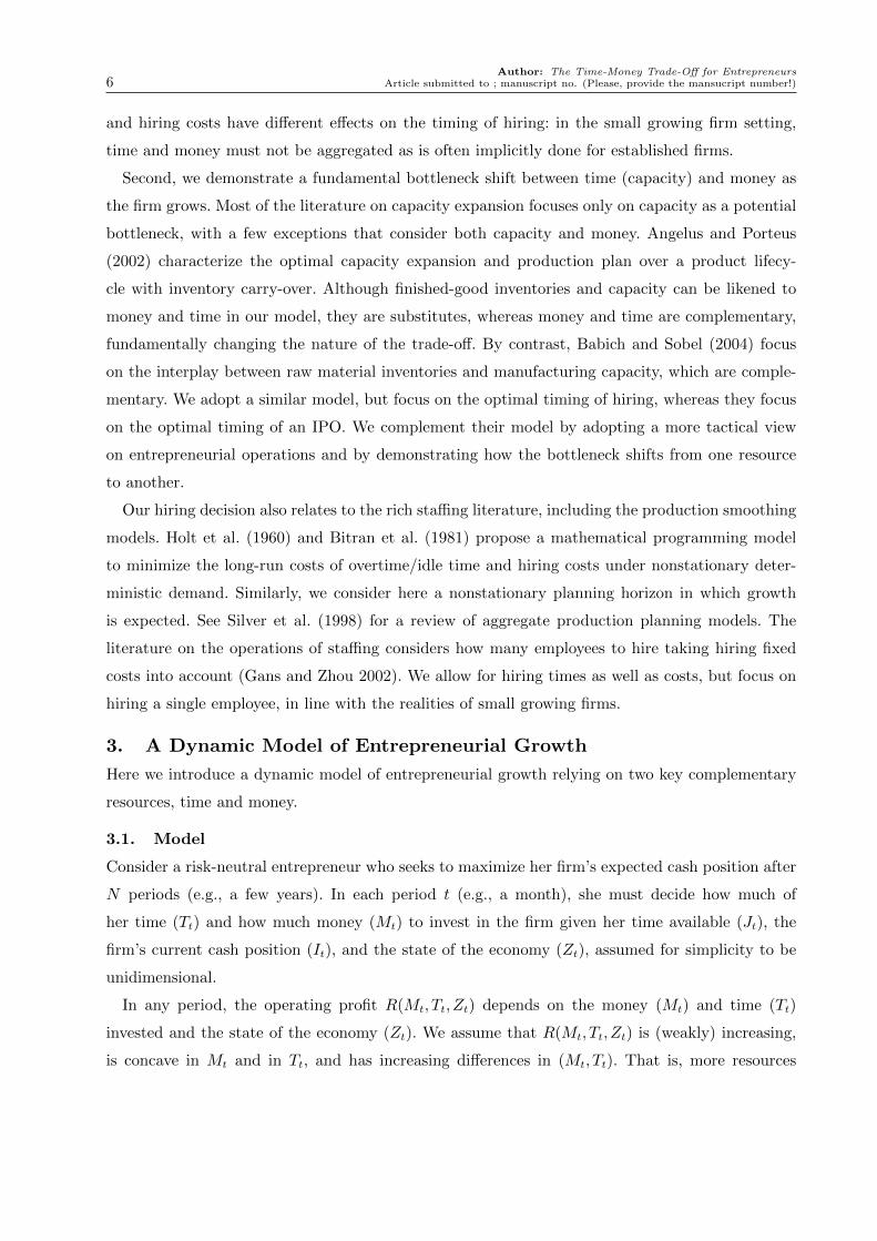
An increase in either the hiring cost (HM) or time (HT ) lowers the revenue in the hiring period

and therefore slows down future growth. If HM increases, delaying hiring is optimal as it postpones

the resource drain to a period where money is less valuable, as shown in Proposition 4(i). By

contrast, the effect of an increase in HT need not be monotone, as shown in Proposition 4(ii). Two

opposing effects are at play. An increase in HT favors delaying hiring in order to postpone incurring

the increased (time) cost of hiring. Conversely, the opportunity cost of time increases over time, so

the entrepreneur would prefer to hire earlier in order to incur the increased hiring time HT earlier

when time is cheaper. This effect is illustrated in Figure 3. The OSLA hiring cash threshold IOSLAH,t

can be increasing in HT (when Z = 0), decreasing in HT (when Z = 30), or decreasing-increasing

in HT (when Z = 10 and Z = 20).

This difference in the effect of hiring cost and time highlights the importance of differentiating

between money and time in early-stage growth-oriented entrepreneurial firms. In classical staffing

models, fixed setup times are often implicitly converted to fixed setup costs. For example, Gans

and Zhou (2002, p. 994) suggest that the fixed hiring cost “typically includes advertising for,

interviewing, and testing of job applicants when appropriate. It may also include one-time training

costs that are independent of wages.” This is appropriate in larger firms, as studied by Gans and

Zhou (2002) and others, but not in our context: if the hiring time were treated as hiring cost, then

one would always delay hiring in response to an increase in hiring time, potentially conflicting with

our prescription.

4.2.3. Optimality of OSLA Hiring Policy. We next show that the OSLA hiring policy,

despite its simplicity, is optimal when the firm grows deterministically, as in staffing planning


models (going back to Holt et al. 1960). In §5, we show numerically that it performs very well even

when growth is not guaranteed.

The first half of Proposition 5 below shows that in a deterministic setting it is never optimal

to hire if the firm’s cash position falls below IOSLAH,t , establishing necessity of the OSLA hiring

threshold condition. The second half shows sufficiency when three assumptions hold: increasing

state of economy, which is common in the entrepreneurship literature (Babich and Sobel 2004) and

the capacity expansion literature (e.g., Luss 1982, Angelus and Porteus 2002); profitability (i.e.,

f(I, J,Zt)≥ I); and constant available time (Jt+k = Jt for all k).

Proposition 5 (Optimality of OSLA Hiring Policy). Suppose that Assumptions 1 and 2

hold true and that |Ωt+k|= 1 for all k≥ 0.

If it is optimal to hire in period t, then It > IOSLAH,t .

Suppose also that (i) Zt+k ≤Zt+k+1 for all k ≥ 0, (ii) f(I, J,Zt)≥ I, and (iii) Jt+k = Jt+k+1 for

all k≥ 0. Then it is optimal to hire in period t if and only if It > IOSLAH,t .

The rationale behind this result is as follows: By Propositions 2 and 3, under growing states

of the economy (Zt) and with constant time available for the entrepreneur (Jt), the OSLA hiring

thresholds are decreasing over time. On the other hand under the specified growth conditions, the

firm’s cash position is increasing over time. As a result, the firm’s cash position will cross the hiring

threshold only once; accordingly, if the OSLA policy prescribes to hire in period t, it will also do

so in all subsequent periods. Effectively, the hiring set is absorbing (Bertsekas 2000).

4.3. Optimal Timing of Firing

We next consider the timing of firing, ignoring the possibility of re-hiring the employee later.

Despite treating hiring and firing separately, we show in §5 that our OSLA hiring and firing policy

performs well in general. By and large, the results mirror those obtained before, thus deepening

the connection between hiring/firing and capacity expansion/contraction. We first characterize the

OSLA firing policy, then study its sensitivity to the model parameters, and finally establish that

it is optimal under certain conditions.

Under the OSLA firing policy, the employee is fired in period t if this increases It+2 more than

firing him in period t+ 1. We assume, in the same spirit as Assumption 1, that firing does not

take any time (FT = 0) and that the firing cost is not too large (for instance, FM ≤w, as shown in

Lemma A-9). These assumptions are sufficient, and not necessary, for the following results to hold.

Based on our interaction with entrepreneurs, firing often does not entail significant time investment

and the only cost is often a severance package, usually no more than one month of salary. Moreover

in §5, we numerically observe that, despite these limited frictions, firing typically only occurs when

the firm is on the verge of going bankrupt and offers only marginal relief.


Assumption 3. FT = 0 and FM is such that gF (I, J,Z)−h(I, J,Z) is decreasing in I.

Under this assumption, the optimal policy can be characterized by two cash thresholds: the

entrepreneur should fire the employee if her cash position is sufficiently low that keeping him one

more period would not be economical, but not so low that the firing cost will cause bankruptcy.

Lemma 3 (OSLA Firing Policy). Suppose that Assumption 3 holds. Define

IOSLA

F,t = maxI| gF (I, Jt,Zt)≥ h(I, Jt,Zt)−FM and IOSLAF,t = minI|gH(I, Jt,Zt)≥L.

The OSLA policy recommends to fire in period t if and only if IOSLAF,t ≤ It ≤ IOSLA

F,t .

The next result mirrors Proposition 5 by demonstrating the optimality of the OSLA firing policy

when the future is deterministic, as often assumed in staffing models (Holt et al. 1960). As before, we

first establish necessity of the OSLA firing cash thresholds, and then, under additional assumptions,

show that they are also sufficient. Contrary to hiring, the optimality of the OSLA firing policy

is established in case of decline, and not growth. (For sensitivity results, see Proposition A-1 in

Appendix.)

Proposition 6 (Optimality of OSLA Firing Policy). Suppose that Assumption 3 holds

and that |Ωt+k|= 1 for all k≥ 0.

If it is optimal to fire in period t, then IOSLAF,t ≤ It ≤ IOSLA

F,t .

Suppose also that (i) either Jt+k = Jt+k+1 for all k≥ 0 or Jt+k ≤ Jt+k+1 for all k≥ 0 and FM ≥w,

(ii) Assumption 2 holds, and (iii) h(I, Jt+k,Zt+k) ≤ I for all k ≥ 0. Then it is optimal to fire in

period t if and only if IOSLAF,t ≤ It ≤ IOSLA

F,t .

If IOSLAH,t ≥ IOSLAF,t , the OSLA hiring-firing policy is similar to the classical “Invest-Stay Put-

Disinvest” policy of capacity expansion (Van Mieghem 2003), under which it is optimal to hire at

high cash levels, keep that employee (stay put) at intermediate levels, and fire that employee at

lower (but not too low) cash levels. (When the cash level is very low, i.e., below IOSLAF,t , it may

be optimal not to fire the employee if incurring the firing cost would precipitate the firm into

bankruptcy.) This result helps further draw the parallel between hiring and capacity expansion.

5. Numerical Analysis

In this section, we show numerically that the OSLA policy is near-optimal and demonstrate its

robustness. We first describe the parameter values used in our experiments, then compare the

OSLA policy with the optimal policy, and finally discuss its robustness.


5.1. Setup and Illustrative Examples

As a base case, we consider an entrepreneur who seeks to maximize the firm’s cash position after

N = 12 months, starting with I0 = $20,000 and working J = 30 days per month. Money can be

borrowed at an annual rate b= 20% with a borrowing limit of κ= 100% of current cash level, similar

to Buzacott and Zhang (2004), so B(M,I,Z) = b[M − I]+ if M ≤ (1 + κ)I and B(M,I,Z) =∞

otherwise. Excess money can be invested at an annual rate of r = 2.5%, and δ = 1/(1 + r). The

entrepreneur is bankrupt when her cash position falls below L= 0, which triggers bankruptcy costs

of K = $100,000, which could roughly represent one year of lost salary while looking for a new job.

We consider a Cobb-Douglas revenue function, similar to Levesque and MacCrimmon (1997),

and additive shocks, so R(M,T,Z) = kMαT β +Z with α< 1. Similar to Babich and Sobel (2004),

we assume that the state of the economy follows a martingale, i.e., Zt+1 = φ(Zt, ωt) = Zt + ωt, in

which ωt is equal to $5,000, −$5,000, or $0 respectively with probability p, q, and 1−p− q. In our

base case, we set Z0 = $0.4 The entrepreneur’s range of uncertainty about the economy increases

with her time horizon, but she may lose or gain up to 25% of her initial endowment (I0) even in

the first period. In our base case, we set p= 0.375 and q = 0.375. We also consider an optimistic

scenario, i.e., p= 0.5 and q= 0.25, and a pessimistic one, i.e., p= 0.25 and q= 0.5.

We assume that, if the entrepreneur were to invest all her initial endowment of time and money,

she would face, in expectation, a return of 5% in the first month, i.e., R(I0, J,Z0)/[(1+r)I0] = 1.05,

which roughly translates into a 180% annual growth rate, not atypical for growing entrepreneurs.

We accordingly set k = 1.05(1 + r)(20)1−αJ−β. In line with Proposition 1, we assume that money

is initially the bottleneck: the money the entrepreneur would like to invest in the business (the

solution to the first-order condition ∂R(M,J,Z)/∂M − (1 + r) = 0) is greater than her initial cash

endowment (I0 = $20,000). Mathematically, we require that (αJβk/(1 + r))1

1−α ≥ $20,000, i.e.,

α≥ 1/1.05≈ 0.95. In our base case, we assume α= 0.99 to ensure that cash will be the bottleneck

for at least a few periods. We consider three values for the elasticity of time: β = 0.7, β = 0.3, and

β = 3. Figure 4 depicts a few representative sample paths of the cash position under this base case,

when β = 0.7, assuming no hiring. The expected initial 5%-growth rate does not always materialize

and certainly does not guarantee the firm’s future growth.

Now assume the entrepreneur can hire an employee, costing w = $6,000 per month and giving

the entrepreneur an extra y = 15 days of time per month to grow the business. Since recruiting

agencies typically collect one or two months of salary, we set HM = $12,000. We assume hiring

takes considerable time, and set HT = 30 days (resulting in available time of 15 days during the

hiring period). By contrast, firing takes no time and costs one month’s severance, so FT = 0 and

4 With different starting points Z0, we set φ(Zt, ωt) = min(N + 1)5,000,max−(N + 1)5,000,Zt + ωt and set anupper bound of $1,000,000 on It to limit the state space while solving the dynamic program.


Figure 4 Sample paths of cash and state of the economy with no hiring.

$k

$50k

$100k

$150k

$200k

$250k

1 2 3 4 5 6 7 8 9 10 11 12

time period

I(t)

Z(t)

‐$15k

‐$10k

‐$5k

$k

$5k

$10k

$15k

$20k

$25k

$30k

$35k

1 2 3 4 5 6 7 8 9 10 11 12

time period

I(t)

Z(t)

‐$80k

‐$60k

‐$40k

‐$20k

$k

$20k

$40k

1 2 3 4 5 6 7 8 9 10 11 12

time period

I(t)

Z(t)

‐$20k

$k

$20k

$40k

$60k

$80k

$100k

1 2 3 4 5 6 7 8 9 10 11 12

time period

I(t)

Z(t)

Figure 5 Distribution of final discounted cash (δNIN) without hiring and hiring via OSLA policy.

FM = $6,000. Note that, even though the derivation of the OSLA policy considers hiring and firing

separately, we consider them jointly here; in particular, the optimal policy to which we benchmark

the OSLA policy could potentially recommend several cycles of hiring and firing.

Is hiring valuable in our setting? Figure 5 plots the histogram of the discounted final cash (δNIN)

without hiring and with the OSLA hiring policy for p= 0.375 and q= 0.375 averaged over 10,000

scenarios. The OSLA policy first-order stochastically dominates the no-hiring policy. Hiring via

the OSLA policy has limited influence on the bankruptcy probability (35.3% vs. 35.4% for no-


Figure 6 Distribution of OSLA hiring times for different levels of economic drifts.

0

0.1

0.2

0.3

0.4

0.5

0.6

0.7

0.8

0 1 2 3 4 5 6 7 8 9 10 11 never

growth (p=0.5, q=0.25)stable (p=0.375, q=0.375)decline (p=0.25, q=0.5)

hiring), but significantly improves the firms chance of higher growth. Without hiring the firm does

not exceed δNIN = 350, but with OSLA-hiring there is a 28% probability of the firm reaching

δNIN = 1000 or higher.

Figure 6 depicts a histogram of the OSLA hiring times in our base case (β = 0.7) under growing,

stable, and declining state of the economy, averaged over 10,000 scenarios. Conditional on hiring

taking place, the median hiring time is period 4 in all three cases, and the mean hiring time is

between 4.5 and 4.7. The probability of hiring is larger if the state of the economy (Zt) has a

positive rather than negative drift, consistent with Proposition 3.

5.2. Performance of OSLA Policy

Tables 1-3 display, for β = 0.7, β = 0.3, and β = 3, the expected cash position in period N (in

$1,000’s), evaluated in period 0, using the optimal hiring policy (V OPT0 ) and using the OSLA

hiring policy (V OSLA0 ) for various starting cash positions and states of the economy. The optimality

gap is defined as ∆ = (V OPT0 − V OSLA

0 )/|V OPT0 |. Overall, the tables show that the OSLA policy

performs very well, typically within a few percent from the optimal policy. In particular, in all

reported instances, the optimality loss is never larger than $3,000. The OSLA policy performs well

because in our setting, (i) time and money investments are expected to generate growth and (ii)

cash accumulation accelerates growth due to the bootstrapping nature. In other settings (e.g., with

limited growth opportunities, negative profitability, or no ability to bootstrap), the OSLA policy

may not work well, but these settings would fundamentally differ from our growth context. Apart

from the obvious computational benefits, the good performance of the OSLA policy implies that

entrepreneurs facing growth opportunities may limit their horizon to one period and still do quite

well.

How sensitive is hiring to the prospect of being able to fire? In our growth setting, it turns out

that firing has very little impact on the performance of both the optimal and the OSLA policy.


p= 0.5, q= 0.25 p= 0.375, q= 0.375 p= 0.25, q= 0.5I0 Z0 V OPT

0 V OSLA0 ∆ V OPT

0 V OSLA0 ∆ V OPT

0 V OSLA0 ∆

20 0 607 606 0.1% 346 345 0.2% 114 114 0.4%20 -10 -18 -19 2.9% -75 -75 0.3% -95 -95 0.1%20 10 977 977 0.0% 974 974 0.0% 962 962 0.0%10 0 472 472 0.2% 215 215 0.4% 26 25 2.2%10 -10 -100 -100 0.0% -100 -100 0.0% -100 -100 0.0%10 10 945 945 0.0% 867 866 0.0% 715 715 0.0%30 0 755 754 0.1% 546 545 0.1% 312 312 0.1%30 -10 55 54 1.7% -48 -48 0.9% -89 -89 0.1%30 10 977 977 0.0% 977 977 0.0% 977 977 0.0%

Table 1 Performance of OSLA hiring policy when β = 0.7

p= 0.5, q= 0.25 p= 0.375, q= 0.375 p= 0.25, q= 0.5I0 Z0 V OPT

0 V OSLA0 ∆ V OPT

0 V OSLA0 ∆ V OPT

0 V OSLA0 ∆

20 0 208 206 0.8% 70 68 2.6% -31 -32 4.6%20 -10 -53 -54 2.3% -84 -84 0.6% -96 -96 0.1%20 10 687 687 0.0% 497 496 0.1% 295 293 0.6%10 0 151 149 1.3% 31 29 5.5% -50 -51 2.0%10 -10 -100 -100 0.0% -100 -100 0.0% -100 -100 0.0%10 10 589 589 0.0% 395 394 0.2% 206 204 1.0%30 0 276 274 0.5% 117 115 1.5% -4 -6 38.4%30 -10 -21 -23 8.9% -71 -72 1.1% -93 -93 0.2%30 10 787 787 0.0% 618 618 0.0% 419 419 0.0%

Table 2 Performance of OSLA hiring policy when β = 0.3

p= 0.5, q= 0.25 p= 0.375, q= 0.375 p= 0.25, q= 0.5I0 Z0 V OPT

0 V OSLA0 ∆ V OPT

0 V OSLA0 ∆ V OPT

0 V OSLA0 ∆

20 0 805 803 0.2% 592 591 0.3% 345 344 0.2%20 -10 104 104 0.5% -29 -29 0.9% -85 -85 0.1%20 10 977 977 0.0% 977 977 0.0% 977 977 0.0%10 0 694 692 0.3% 417 415 0.5% 152 151 0.7%10 -10 -100 -100 0.0% -100 -100 0.0% -100 -100 0.0%10 10 977 977 0.0% 977 977 0.0% 977 977 0.0%30 0 977 977 0.0% 977 977 0.0% 977 977 0.0%30 -10 237 236 0.4% 35 34 1.6% -64 -64 0.2%30 10 977 977 0.0% 977 977 0.0% 977 977 0.0%

Table 3 Performance of OSLA hiring policy when β = 3

Table 4 reports the discounted final cash δNIN of the optimal policy and the OSLA policy both

when firing is frictionless (FM = FT = 0) and when firing is not allowed, in our base case of hiring

frictions (HM = $12,000 and HT = 30 days) as well as when hiring is frictionless (HM =HT = 0),

when β = 0.7, p = q = 0.375. As shown in the table, not allowing firing only leads to a marginal

decline in performance. On the other hand, hiring frictions significantly affect performance.

Firing has little impact on performance here primarily because of our growth assumptions. In

that setting, hiring accelerates growth; as a result, it is unlikely that, if the firm has hired an


HM = $12,000, HT = 30 days HM = $0, HT = 0 daysFrictionless Firing No Firing Frictionless Firing No Firing

I0 Z0 V OPT0 V OSLA

0 ∆ V OPT0 V OSLA

0 ∆ V OPT0 V OSLA

0 ∆ V OPT0 V OSLA

0 ∆20 0 346 346 0.2% 346 345 0.2% 977 977 0.0% 977 977 0.0%20 -10 -75 -75 0.3% -75 -75 0.3% 118 118 0.0% 108 108 0.0%20 10 974 974 0.0% 974 974 0.0% 977 977 0.0% 977 977 0.0%10 0 216 215 0.4% 215 215 0.4% 475 475 0.0% 474 474 0.1%10 -10 -100 -100 0.0% -100 -100 0.0% -100 -100 0.0% -100 -100 0.0%10 10 867 866 0.0% 867 866 0.0% 977 977 0.0% 977 977 0.0%30 0 546 545 0.1% 546 545 0.1% 977 977 0.0% 977 977 0.0%30 -10 -48 -48 0.9% -48 -48 0.9% 977 977 0.0% 977 977 0.0%30 10 977 977 0.0% 977 977 0.0% 977 977 0.0% 977 977 0.0%

Table 4 Performance of OSLA hiring policy with and without hiring frictions when β = 0.7, p= q= 0.375

employee, it would need to fire her at some point. Moreover, the state of the economy must be low

if the firm needs to fire her employee. Given that successive states of the economy are positively

correlated here, this implies that future states of the economy may also be low, and therefore

that firing rarely helps avert going bankrupt. Given the low impact of firing on performance, we

therefore conclude that treating them separately, as we did in our derivation of the OSLA policy

in §4, can be done with no great loss of optimality when considering a growth-oriented firm, unlike

established firms (Bentolila and Bertola 1990).

The sensitivity of both the OSLA and the optimal policies with respect to bankruptcy costs

K is shown in Tables 5 and 6. Specifically, we consider K = $10,000,000 and K = $0 (the base

case takes K = $100,000). We observe a marginal deterioration in the OSLA performance when

the bankruptcy cost is large and when the chance that the firm will not go bankrupt is moderate.

(Even when the relative optimality loss may appear large, as when I0 = $30,000, Z0 = $0, p= 0.5,

and q = 0.25 in Table 5, the absolute loss remains small, especially compared to the $10,000,000-

bankruptcy cost.) If it is clear that the firm will go bankrupt, then OSLA performs as poorly as

the optimal policy; and if it is clear that the firm will not go bankrupt, then the bankruptcy cost

has minimal influence.

5.3. Robustness

How robust are the OSLA thresholds to the model parameters? Table 7 displays the OSLA hiring

and firing thresholds for different values of the money and time elasticities α and β and different

values of Zt.5 Consistent with Proposition 3, the hiring thresholds are increasing in Zt. (The

firing upper thresholds are independent of Zt, consistent with Proposition A-1 in the Appendix.)

Moreover, the dependence of the hiring cash threshold on Zt appears almost linear, so IOSLAH,t should

5 Because the OSLA hiring policy does not consider firing and vice versa, the OSLA hiring cash threshold need notbe larger than the OSLA firing threshold, as when Zt is large. This does not mean that the entrepreneur should hireto fire: Zt is so large that the cash position after hiring will likely be above the firing threshold.


p= 0.5, q= 0.25 p= 0.375, q= 0.375 p= 0.25, q= 0.5I0 Z0 V OPT

0 V OSLA0 ∆ V OPT

0 V OSLA0 ∆ V OPT

0 V OSLA0 ∆

20 0 -711 -727 2.3% -3,204 -3,237 1.0% -6,302 -6,335 0.5%20 -10 -7,583 -7,585 0.0% -9,034 -9,037 0.0% -9,736 -9,737 0.0%20 10 977 977 0.0% 974 974 0.0% 962 962 0.0%10 0 -1,561 -1,571 0.6% -4300 -4,323 0.5% -7,232 -7,259 0.4%10 -10 -9,961 -9,961 0.0% -9,961 -9,961 0.0% -9,961 -9,961 0.0%10 10 885 880 0.5% 464 448 3.4% -727 -749 3.1%30 0 -76 -113 49.7% -1,998 -2,049 2.6% -4,754 -4,788 0.7%30 -10 -5,980 -5,987 0.1% -8,258 -8,266 0.1% -9,499 -9,504 0.0%30 10 977 977 0.0% 977 977 0.0% 977 977 0.0%

Table 5 Performance of OSLA hiring policy when β = 0.7 and K = $10,000,000

p= 0.5, q= 0.25 p= 0.375, q= 0.375 p= 0.25, q= 0.5I0 Z0 V OPT

0 V OSLA0 ∆ V OPT

0 V OSLA0 ∆ V OPT

0 V OSLA0 ∆

20 0 621 620 0.1% 382 382 0.1% 179 179 0.1%20 -10 58 58 0.9% 15 15 1.5% 2 2 2.2%20 10 977 977 0.0% 974 974 0.0% 962 962 0.0%10 0 493 492 0.1% 261 260 0.3% 99 99 0.3%10 -10 0 0 0.0% 0 0 0.0% 0 0 0.0%10 10 946 946 0.0% 871 871 0.0% 729 729 0.0%30 0 764 763 0.0% 572 571 0.1% 364 364 0.0%30 -10 116 115 0.8% 35 35 1.1% 6 6 1.4%30 10 977 977 0.0% 977 977 0.0% 977 977 0.0%

Table 6 Performance of OSLA hiring policy when β = 0.7 and K = $0

α βZt

-60 -50 -40 -30 -20 -10 0 10 20 30 40 50 60

IOSLAH,t

0.99 0.7 94 84 74 64 53 43 33 22 12 1 1 1 10.99 0.3 108 98 88 77 66 56 45 34 23 11 1 1 10.99 3 86 76 66 56 46 35 25 15 6 1 1 1 10.8 0.7 90 80 70 60 50 40 30 20 12 1 1 1 1

IOSLA

F,t

0.99 0.7 12 12 12 12 12 12 12 12 12 12 12 12 120.99 0.3 23 23 23 23 23 23 23 23 23 23 23 23 230.99 3 6 6 6 6 6 6 6 6 6 6 6 6 60.8 0.7 12 12 12 12 12 12 12 12 12 12 12 12 12

Table 7 OSLA hiring and firing cash thresholds when p= q= 0.375

not be too sensitive to the variance of Zt if its mean is properly estimated. Furthermore, IOSLAH,t

appears relatively robust to misspecifications of α and β, at least up to a limit: when the time

elasticity falls below a certain level (e.g., when β ≤ 0.5 if α= 0.8), the hiring threshold jumps to

infinity, so it becomes optimal to never hire.

The high performance of the OSLA policy raises the question: How important is the timing of

hiring? What are the consequences of hiring too early or too late? To address this question, we

conduct the following experiment. For all t, we evaluate the expected revenue δNIN , averaged over

10,000 simulation runs, with an OSLA policy when the hiring cash thresholds are perturbed, i.e.,


Figure 7 Relative losses in optimality when the hiring cash thresholds are perturbed.

‐20%

0%

20%

40%

60%

80%

100%

120%

140%

160%

180%

‐10 ‐9 ‐8 ‐7 ‐6 ‐5 ‐4 ‐3 ‐2 ‐1 0 1 2 3 4 5 6 7 8 9 10

Perturbation

p=0.5 q=0.25

p=0.375 q=0.375

p=0.25 q=0.5

‐20%

0%

20%

40%

60%

80%

100%

120%

140%

‐10 ‐9 ‐8 ‐7 ‐6 ‐5 ‐4 ‐3 ‐2 ‐1 0 1 2 3 4 5 6 7 8 9 10

Perturbation

p=0.5 q=0.25

p=0.375 q=0.375

p=0.25 q=0.5

Note. (HM ,HT ) = ($12,000,30 days) (left) and (HM ,HT ) = ($6,000,15 days) (right).

by using IOSLAH,t + π, for all t, π =−10, · · · ,+10. Figure 7 depicts the relative loss of revenue from

using cash thresholds IOSLAH,t +π instead of IOSLAH,t , when p= 0.5 and q= 0.25 (solid), p= 0.375 and

q = 0.375 (dashed), and p= 0.25 and q = 0.5 (dotted) for high hiring cost and time (left) and low

hiring cost and time (right).

Overall, the figure shows that the hiring cash thresholds are relatively robust when the cash

thresholds are overestimated. By contrast, underestimating the hiring cash thresholds can lead

to a significant loss of revenue. The risks involved in hiring are highly asymmetric: while hiring

too late (high IOSLAH,t ) hurts performance only moderately, hiring too early (low IOSLAH,t ) can have

severe consequences, potentially precipitating the entrepreneur into bankruptcy. The asymmetry

in the optimality loss curve is consistent with our result that in a deterministic environment the

OSLA hiring cash threshold is a lower bound on the optimal hiring threshold (Proposition 5(i)).

Overall, Figure 7 indicates that the optimal threshold is relatively insensitive to perturbations, so

reasonable approximations such as the OSLA cash threshold should perform well.

6. Conclusions

In this paper, we study how growth in small entrepreneurial firms is affected by two key constraints:

money and time. The two resources are asymmetric in that (i) money, unlike time, is fungible, and

(ii) the primary output of the firm is money, not time. We introduce a model of growth, which

depends on complementary inputs of money and time, explore the consequences of this asymmetry,

and how entrepreneurs can trade time and money.

First, we establish that as the firm grows, there is a fundamental shift in the bottleneck from

money to time. Hiring is then a natural mechanism to trade off less valuable money for more

valuable time, thereby increasing capacity to accelerate growth.

Second, we characterize the timing of hiring in terms of a cash level threshold via a one-stage-

look-ahead (OSLA) policy. We numerically demonstrate that this OSLA policy performs well and

show that it is optimal under deterministic growth. The high performance of the OSLA policy is


driven by the growth conditions and bootstrapping strategy inherent in our context. This suggests

that the hiring of subsequent employees may also be timed in an OSLA fashion, similar to the

timing of the first employee, provided that these growth conditions continue to hold.

Unlike established firm settings of capacity expansion or staffing, for growth-oriented firms, the

entrepreneur’s time is critical for growth and thus cannot implicitly be converted into money. In

particular, we show that unlike hiring costs, which always delay the timing of hiring, greater hiring

times may delay or expedite the timing of hiring. This is due to two opposing effects: an increase

in hiring time yields slower growth pushing for hiring later, but the entrepreneur wants to incur

the higher hiring time when her time is less valuable, pushing for hiring earlier.

To sustain growth, entrepreneurs must effectively marshal their key resources, such as time and

money. Managing operations in these growth settings requires properly identifying the bottleneck

resource at specific points in time and putting in place strategies to alleviate them.

References

Aldrich, H.E., C.M. Fiol. 1994. Fools rush in? The institutional context of industry creation. Academy of

Management Review. 19(4), 645–670.

Angelus, A., E.L. Porteus. 2002. Simultaneous capacity and production management of short-life-cycle,

produce-to-stock goods under stochastic demand. Management Science. 48(3), 399-413.

Archibald, T.W., L.C. Thomas, J.M. Betts, R.B. Johnston. 2002. Should start-up companies be cautious?

Inventory policies which maximize survival probabilities. Management Science, 48(9) 1161-1174.

Babich, V., M.J. Sobel. 2004. Pre-IPO operational and financial decisions. Management Science 50(7), 935-

948.

Bentolila, S., G. Bertola. 1990. Firing costs and labour demand: How bad is Eurosclerosis? The Review of

Economic Studies, 57(3), 381–402.

Berger, A. N., G. F. Udell. 1998. The economics of small business finance: The role of private equity and

debt markets in the financial growth cycle. Journal of Banking and Finance, 22(6-8), 613–673.

Bertsekas, D.P. 2000. Dynamic Programming and Optimal Control, Volume 1. Athena Scientific, Belmont,

MA. Second Edition.

Bitran, G.R., E.A. Haas, A.C. Hax. 1981. Hierarchical production planning: A single stage system. Operations

Research, 29(4), 717–743.

Boyd, S., L. Vandenberghe. 2004. Convex Optimization. Cambridge University Press, Cambridge, UK.

Burgstone, J. and Murphy Jr, B. 2012. Breakthrough Entrepreneurship. Farallon Publishing. San Francisco,

CA.

Buzacott, J.A., R.Q. Zhang. 2004. Inventory management with asset-based financing. Management Science,

50(9), 1274–1292.


Caldentey, R., M. Haugh. 2006. Optimal control and hedging of operations in the presence of financial

markets. Mathematics of Operations Research. 31(2), 285–304.

Churchill, N.C., V.L. Lewis. 1983. The five stages of small business growth. Harvard Business Review, May–

June, 1983.

Collins, C.J., K.D. Clark. 2003. Strategic human resource practices, top management team social networks,

and firm performance: The role of human resource practices in creating organizational competitive

advantage. Academy of Management Journal, 46(6), 740–751.

Cressy, R. 1996. Are business startups debt-rationed?. The Economic Journal, 106(438), 1253–1270.

Dada, M., Q. Hu. 2008. Financing newsvendor inventory. Operations Research Letters, 36(5), 569–573.

Dixit, A.K., R.S. Pindyck. 1994. Investment Under Uncertainty. Princeton University Press, Princeton, NJ.

Dupuy, A., A. de Grip. 2006. Elasticity of substitution and productivity, capital and skill intensity differences

across firms. Economic Letters 90(3), 340–347.

Ebben, J., A. Johnson. 2006. Bootstrapping in small firms: An empirical analysis of change over time. Journal

of Business Venturing, 21(6), 851–865.

Evans, D.S., B. Jovanovic. 1989. An estimated model of entrepreneurial choice under liquidity constraints.

Journal of Political Economy, 97(4), 808–827.

Gans, N., Y.P. Zhou. 2002. Managing learning and turnover in employee staffing. Operations Research, 50(6),

991–1006.

Garmaise, M. J.. 2008. Production in entrepreneurial firms: The effects of financial constraints on labor and

capital. The Review of Financial Studies, 21(2), 543–577.

Gifford, S. 1992. Allocation of entrepreneurial attention. Journal of Economic Behavior and Organization,

19(3), 256–284.

Goldratt, E. M.. 2004. The Goal: A Process of Ongoing Improvement. North River Press.

Hambrick, D.C., L.M. Crozier. 1985. Stumblers and stars in the management of rapid growth. Journal of

Business Venturing, 1(1), 31–45.

Hamermesh, R.G., J.L. Heskett, M.J. Roberts. 2005. A note on managing the growing venture. Harvard

Business School Case, 9-805-092.

Hess, E.D. 2012. Grow to Greatness. Stanford University Press. Stanford, CA.

Holt, C.C., F. Modigliani, J.F. Muth, H.A. Simon. 1960. Planning Production, Inventories, and Workforce.

Prentice-Hall, Englewood Cliffs, NJ.

Hu, Q., M. Sobel. 2005. Capital structure and inventory management. Case Western University Working

Paper.

Jovanovic, B. 1982. Selection and the evolution of industry. Econometrica, 50(3), 649–670.


Kouvelis, P., W. Zhao. 2011. The newsvendor problem and price-only contract when bankruptcy costs exist.

Production and Operations Management, 26(6), 921–936.

Krishnan, V. 2013. Operations management opportunities in technology commercialization and entrepreneur-

ship. Production and Operations Management, Forthcoming.

Levesque, M., C. Schade. 2005. Intuitive optimizing: Experimental findings on time allocation decisions with

newly formed ventures. Journal of Business Venturing, 20(3), 313–342.

Levesque, M., K. MacCrimmon. 1997. On the interaction of time and money invested in new ventures.

Entrepreneurship Theory and Practice, 22(2), 89–110.

Li, L. 1988. A stochastic theory of the firm. Mathematics of Operations Research, 13(3), 447–466.

Li, L, M. Shubik, M. Sobel. 2009. Control of dividends, capital subscriptions, and physical inventories. Case

Western Reserve University Working Paper.

Luss, H. 1982. Operations research and capacity expansion problems: A survey. Operations Research, 30(5),

907–947.

Manne, A. 1961. Capacity expansion and probabilistic growth. Econometrica, 29(4), 632–649.

Martin, B., T. Papadimitriou. 2009. Are You the Bottleneck in Your Organization? Retrieved December 8,

2009, from http://blogs.hbr.org/cs/2009/12/

Mueler, S., Volery, T., and von Siemens, B. 2012. What do entrepreneurs actusally do? An observational

study of entrepreneurs’ everyday behavior in the start-up and growth stages. Entrepreneurship Theory

and Practice, 36(5), 995–1017.

Phillips, B.D., B.A. Kirchhoff. 1989. Formation, growth and survival. Small firm dynamics in the US economy.

Small Business Economics, 1(1), 65–74.

Quinn, R.E., K. Cameron. 1983. Organizational life cycles and shifting criteria of effectiveness: Some pre-

liminary evidence. Management Science, 29(1), 33–51.

Radner, R., L. Shepp. 1996. Risk vs. profit potential: A model for corporate strategy. Journal of Economic

Dynamics and Control, 20(8), 1373–1393.

Shepp, L., A. Shiryaev. 1996. Hiring and firing optimally in a large corporation. Journal of Economic Dynam-

ics and Control, 20(9-10), 1523–1539.

Silver, E.A., D.F. Pyke, R. Peterson. 1998. Inventory Management and Production Planning and Scheduling.

John Wiley & Sons, New York, NY.

Sobel, M., D. Turcic. 2007. Coordination of inventory, capital and dividends in nascent firms. Case Western

Reserve University Working Paper.

Swinney, R., G. Cachon, S. Netessine. 2011. Capacity investment timing by start-ups and established firms

in new markets. Management Science, 57(4), 763–777.


Tanrisever, F., S. Erzurumulu, N. Joglekar. 2012. Production, process improvement and the survival of debt

fincanced startup firms. Production and Operations Management, Forthcoming.

Tansky, J.W., R.L. Heneman. 2006. Human Resource Strategies for the High Growth Entrepreneurial Firm.

Information Age Publishing, Inc., Greenwich, CT.

Topkis, D.M. 1998. Supermodularity and Complementarity. Princeton University Press, New Jersey.

Van Mieghem, J.A. 2003. Capacity management, investment, and hedging: Review and recent developments.

Manufacturing & Service Operations Management, 5(4), 269–302.

Williamson, I.O. 2000. Employer legitimacy and recruitment success in small business. Entrepreneurship:

Theory and Practice, 25: 27–42.

Xu, X., J. Birge. 2006. Equity valuation, production, and financial planning: A stochastic programming

approach. Naval Resarch Logistics, 53(7), 641–655.

Ye, Q., I. Duenyas. 2007. Optimal capacity investment decisions with two-sided fixed capacity adjustment

costs. Operations Research, 55(2): 272-284.

Yoo, O.S., C.J. Corbett, G. Roels. 2011. Dynamic Process Improvement for Growth: Optimal Time Allocation

Policy for Entrepreneurs. Working Paper.

Appendix

Lemma A-1. V 0t (It, Jt,Zt) is increasing in It.

Proof. The proof is by induction on t. By (1), when t=N , V 0N(IN , JN ,ZN) = IN if IN >L and it is equal

to −K otherwise. Fix t and suppose that V 0t+1(It+1, Jt+1,Zt+1) is increasing in It+1. Let I+ > I−. Suppose

that I− ≥L. Then, using (1),

V 0t (I+, Jt,Zt) = max

Mt,Tt≤JtδEωt

[V 0t+1((1 + r)I+ + Π(Mt, Tt|I+,Zt), Jt+1, φt(Zt, ωt)

]≥ max

Mt,Tt≤JtδEωt

[V 0t+1((1 + r)I−+ Π(Mt, Tt|I−,Zt), Jt+1, φt(Zt, ωt)

]= V 0

t (I−, Jt,Zt),

in which the inequality follows by induction hypothesis and because Π(Mt, Tt|I,Zt) is increasing in I since

B(M,I,Z) is decreasing in I. If I− < L, then V 0t (I−, Jt,Zt) = −K ≤ V 0

t (I+, Jt,Zt) by assumption on K,

with equality only if I+ <L.

Proof of Lemma 1. By Lemma A-1, maximizing δEωt

[V 0t+1((1 + r)It + Π(Mt, Tt|It,Zt), Jt+1, φt(Zt, ωt)

]with respect to (Mt, Tt) is equivalent to maximizing Π(Mt, Tt|It,Zt).

Lemma A-2. (i) Π∗(I, J,Z) has increasing differences in (I, J); (ii) Π∗(I, J,Z) is concave increasing in

(I, J).

Proof. (i) The function Π(M,T |I,Z) is supermodular in (M,T, I) since the sum of supermodular func-

tions is supermodular (Lemma 2.6.1 in Topkis 1998) and since (i) R(M,T,Z) is supermodular in (M,T ), (ii)

B(M,I,Z) is submodular in (M,I), (iii) [M − I]+ is submodular in (M,−I) since it is a convex increasing


transformation of an isotone valuation in (M,I) by Lemma 2.6.4 in Topkis (1998). Because Π(M,T |I,Z) is

supermodular in (M,T, I), and because the feasible set of T is increasing in J respectively, the result follows

from Theorem 2.7.6 in Topkis (1998).

(ii) When maximized over T ≤ J , Π(M,T |I,Z) = Π(M,J |I,Z) since Π(M,T |I,Z) is increasing in J . The

function Π(M,J |I,Z) is concave in (M,J, I) since B(M,I,Z) is convex in (M,I) and R(M,J,Z) is concave

in (M,J). Because concavity is preserved under maximization over convex sets (Boyd and Vandenberghe

2004), Π∗(I, J,Z) is concave in (I, J).

Proof of Proposition 1. To simplify notations, we assume that Π∗(I, J,Z) is differentiable in (I, J). Apply-

ing the chain rule to (1) and using Lemma 1, we obtain:

τt =∂

∂JV 0t (It, Jt,Zt)

= δ∂

∂IEωt

[V 0t+1((1 + r)It + Π∗(It, Jt,Zt), Jt+1, φt(Zt, ωt))

] ∂∂J

Π∗(It, Jt,Zt), and

µt =∂

∂IV 0t (It, Jt,Zt)− δ

∂

∂IEωt

[V 0t+1(It+1, Jt+1, φt(Zt, ωt))

]= δ

∂

∂IEωt

[V 0t+1((1 + r)It + Π∗(It, Jt,Zt), Jt+1, φt(Zt, ωt))

] ∂∂I

Π∗(It, Jt,Zt).

Hence µt > τt if and only if ∂Π∗(It, Jt,Zt)/∂It − ∂Π∗(It, Jt,Zt)/∂Jt > 0. Because Π∗(I, J,Z) is concave in

(I, J) and has increasing differences in (I, J) by Lemma A-2, the left-hand side is decreasing in It and increas-

ing in Jt. When It <L, Mt = 0 for otherwise B(Mt, It,Zt) =∞ by assumption, and therefore Π∗(It, Jt,Zt) =

R(0, Jt,Zt) =R(0,0,Zt). Hence, ∂Π∗(It, Jt,Zt)/∂It = 0 for all It <L, and the left-hand side is nonnegative

by Lemma A-2(ii). On the other hand, when It→∞, Π∗(It, Jt,Zt) = maxMt,Tt≤Jt R(Mt, Tt,Zt)− (1 + r)Mt

since limI→∞B(M,I,Z)≤B(M,M,Z) = 0. Hence, limIt→∞ ∂Π∗(It, Jt,Zt)/∂It = 0, and the left-hand side is

nonpositive by Lemma A-2(ii). Hence, there exists a cash threshold I such that τt <µt if and only if It < I.

When Jt = 0, ∂Π∗(It, Jt,Zt)/∂It = 0 since Π∗(It,0,Zt) = maxMtR(M,0,Zt)− (1 + r)M − B(M,I,Zt) +

(1 + r)[M − I]+ ≤R(0,0,Zt); in that case, the left-hand side is nonpositive by Lemma A-2(ii). On the other

hand, when Jt→∞, ∂Π∗(It, Jt,Zt)/∂Jt = 0, and the left-hand side is nonnegative by Lemma A-2(ii). Hence,

there exists a time threshold J such that τt <µt if and only if Jt > J .

Lemma A-3. Vt(Et, It,Zt) is increasing in It.

Proof. The proof is similar to the proof of Lemma A-1.

Lemma A-4. For any y≥HT , gH(I, J,Z)− f(I, J,Z) is increasing in I and decreasing in J .

Proof. Define y ≡ y−HT ≥ 0 and w≡w+HM ≥ 0. Fix ε > 0. By Lemma A-2, Π∗(I, J,Z) is concave in

I and has increasing differences in (I, J). Accordingly,

Π∗(I + ε−w,J + y,Z)−Π∗(I −w,J + y,Z) ≥ Π∗(I + ε, J + y,Z)−Π∗(I, J + y,Z)

≥ Π∗(I + ε, J,Z)−Π∗(I, J,Z).

Hence, Π∗(I, J,Z)−Π∗(I −w,J + y,Z)≥Π∗(I + ε, J,Z)−Π∗(I + ε−w,J + y,Z), i.e., Π∗(I, J,Z)−Π∗(I −w,J + y,Z) is decreasing in I. Using the fact that Π∗(I, J,Z) is concave in I and has increasing differences

in (I, J) by Lemma A-2, the proof that Π∗(I, J,Z)−Π∗(I −w,J + y,Z) is increasing in J follows a similar

argument.


Lemma A-5. If f(I, Jt,Zt) ≤ gH(I, Jt,Zt) + HM , then gH(f(It, Jt,Zt), Jt+1,Zt+1) ≤

h(gH(It, Jt,Zt), Jt+1,Zt+1).

Proof. We have:

gH(f(It, Jt,Zt), Jt+1,Zt+1)−h(gH(It, Jt,Zt), Jt+1,Zt+1) (A-1)

= (1 + r)(f(It, Jt,Zt)−w−HM)− (1 + r)(gH(It, Jt,Zt)−w)

+Π∗ (f(It, Jt,Zt)−w−HM , Jt+1 + y−HT ,Zt+1)−Π∗ (gH(It, Jt,Zt)−w,Jt+1 + y,Zt+1)

≤ Π∗ (gH(It, Jt,Zt)−w,Jt+1 + y−HT ,Zt+1)−Π∗ (gH(It, Jt,Zt)−w,Jt+1 + y,Zt+1)≤ 0, (A-2)

in which the first inequality follows because Π∗(I, J,Z) is increasing in I by Lemma A-2 and since

f(It, Jt,Zt)≤ gH(It, Jt,Zt) +HM , and the second inequality follows because Π∗(I, J,Z) is increasing in J by

Lemma A-2.

Lemma A-6. Under Assumption 1, when f(It, Jt,Zt)≥ gH(It, Jt,Zt) +HM , gH(f(It, Jt,Zt), Jt+1,Zt+1)−

h(gH(It, Jt,Zt), Jt+1,Zt+1) is decreasing in It.

Proof. We use equation (A-1). By Assumption 1, f(I, J, z)− gH(I, J,Z) is decreasing in I. Fix ε > 0. By

Lemma A-2, Π∗(I, J,Z) has increasing differences in (I, J) and is concave increasing in I. Hence,

Π∗ (gH(It + ε, Jt,Zt)−w,Jt+1 + y,Zt+1)−Π∗ (gH(It, Jt,Zt)−w,Jt+1 + y,Zt+1)

≥ Π∗ (gH(It + ε, Jt,Zt)−w,Jt+1 + y−HT ,Zt+1)−Π∗ (gH(It, Jt,Zt)−w,Jt+1 + y−HT ,Zt+1)

≥ Π∗ (f(It + ε, Jt,Zt) + gH(It, Jt,Zt)− f(It, Jt,Zt)−w,Jt+1 + y−HT ,Zt+1)

−Π∗ (gH(It, Jt,Zt)−w,Jt+1 + y−HT ,Zt+1)

≥ Π∗ (f(It + ε, Jt,Zt)−w−HM , Jt+1 + y−HT ,Zt+1)−Π∗ (f(It, Jt,Zt)−w−HM , Jt+1 + y−HT ,Zt+1) ,

in which the first inequality follows because g(I, J,Z) is increasing in I and because Π∗(I, J,Z) is increasing in

I and has increasing differences in (I, J); the second is because Π∗(I, J,Z) is increasing in I and gH(It, Jt,Zt)−

f(It, Jt,Zt) is increasing in It by Assumption 1; and the last inequality follows because Π∗(I, J,Z) is con-

cave in I and f(It, Jt,Zt) ≥ gH(It, Jt,Zt) + HM . Hence, Π∗ (f(It, Jt,Zt)−w−HM , Jt+1 + y−HT ,Zt+1) −

Π∗ (gH(It, Jt,Zt)−w,Jt+1 + y,Zt+1) is decreasing in It.

Proof of Lemma 2. Suppose that It > IOSLAH,t . Because Π∗(I, J,Z) is increasing in I by Lemma A-

2, gH(It, Jt,Zt) ≥ L. By Assumption 1, there exists a threshold I such that gH(I, Jt,Zt) + HM >

f(I, Jt,Zt) if and only I > I. We consider two cases. First, suppose that It ≥ I. Then, by Lemma A-5,

gH(f(It, Jt,Zt), Jt+1,Zt+1)≤ h(gH(It, Jt,Zt), Jt+1,Zt+1) for all Zt+1. Second, suppose that It ≤ I, and there-

fore, that IOSLAH,t < I. Then, by Lemma A-6,

Eωt[gH(f(It, Jt,Zt), Jt+1, φt(Zt, ωt))−h(gH(It, Jt,Zt), Jt+1, φt(Zt, ωt))]

≤ Eωt[gH(f(IOSLAH,t , Jt,Zt), Jt+1, φt(Zt, ωt))−h(gH(IOSLAH,t , Jt,Zt), Jt+1, φt(Zt, ωt))]≤ 0.

Hence, hiring in period t maximizes It+2. The proof for the case in which It < IOSLAH,t is similar.


Proof of Proposition 2. The proof applies the implicit function theorem to the equations defining IOSLAH,t .

Suppose that gH(IOSLAH,t , Jt,Zt) =L. Then, IOSLAH,t is independent of Jt+1.

Suppose next that G(IOSLAH,t , Jt+1) ≡ Eωt[gH(f(IOSLAH,t , Jt,Zt), Jt+1, φt(Zt, ωt)) −

h(gH(IOSLAH,t , Jt,Zt), Jt+1, φt(Zt, ωt))] = 0. By Lemma A-5, we must have that gH(IOSLAH,t , Jt,Zt) + HM ≤f(IOSLAH,t , Jt,Zt). Hence by Lemma A-6, G(IOSLAH,t , Jt+1) is decreasing in It. For each ωt ∈ Ωt, when

gH(I, Jt,Zt) +HM ≤ f(I, Jt,Zt), we have

∂gH(f(I, Jt,Zt), Jt+1, φt(Zt, ωt))

∂J− ∂h(gH(I, Jt,Zt), Jt+1, φt(Zt, ωt))

∂J

=∂Π∗(f(I, Jt,Zt)−HM −w,Jt+1 + y−HT , φt(Zt, ωt))

∂J− ∂Π∗(gH(I, Jt,Zt)−w,Jt+1 + y,φt(Zt, ωt))

∂J

≥ ∂Π∗(gH(I, Jt,Zt)−w,Jt+1 + y−HT , φt(Zt, ωt))


∂J

≥ ∂Π∗(gH(I, Jt,Zt)−w,Jt+1 + y,φt(Zt, ωt))


∂J≥ 0,

in which the first inequality follows because Π∗(I, J,Z) has increasing differences in (I, J) by Lemma A-2 and

because f(It, Jt,Zt)≥ gH(It, Jt,Zt) +HM ; and the second inequality follows because Π∗(I, J,Z) is concave

in J by Lemma A-2. Hence, G(IOSLAH,t , Jt+1) is increasing in Jt+1.

Suppose now that HT = HM = 0 and L = −∞. Suppose that Eωt[gH(f(IOSLAH,t , Jt,Zt), Jt+1, φt(Zt, ωt))−

h(gH(IOSLAH,t , Jt,Zt), Jt+1, φt(Zt, ωt))] = 0, i.e., G(IOSLAH,t , Jt) ≡ f(IOSLAH,t , Jt,Zt) − h(IOSLAH,t , Jt,Zt) = 0 since

gH(.) = h(.). Since Π(I, J,Z) is concave in I and has increasing differences in (I, J), G(IOSLAH,t , Jt) is decreasing

in I and increasing in Jt, i.e., IOSLAH,t is increasing in Jt.


Suppose that IOSLAH,t solves gH(I, Jt,Zt) =L. Because the left-hand side is increasing in I by Lemma A-2 and

increasing in Z, we obtain that dIOSLAt /dZt ≤ 0.

Suppose next that G(IOSLAH,t , Jt+1) ≡ Eωt[gH(f(IOSLAH,t , Jt,Zt), Jt+1, φt(Zt, ωt)) −

h(gH(IOSLAH,t , Jt,Zt), Jt+1, φt(Zt, ωt))] = 0. By Lemma A-5, we must have that gH(IOSLAH,t , Jt,Zt) + HM ≤f(IOSLAH,t , Jt,Zt). Hence by Lemma A-6, G(IOSLAH,t , Jt+1) is decreasing in It. For each ωt ∈ Ωt, when

gH(I, Jt,Zt) +HM ≤ f(I, Jt,Zt), we have

∂gH(f(I, Jt,Zt), Jt+1, φt(Zt, ωt))

∂I

∂f(I, Jt,Zt)

∂Z− ∂h(gH(I, Jt,Zt), Jt+1, φt(Zt, ωt))

∂I

∂gH(I, Jt,Zt)

∂Z

+∂φt(Zt, ωt)

∂Z

(∂gH(f(I, Jt,Zt), Jt+1, φt(Zt, ωt))

∂Z− ∂h(gH(I, Jt,Zt), Jt+1, φt(Zt, ωt))

∂Z

)=∂gH(I, Jt,Zt)

∂Z

(∂Π∗(f(I, Jt,Zt)−w−HM , Jt+1 + y−HT , φt(Zt, ωt))

∂I− ∂Π∗(gH(I, Jt,Zt)−w,Jt+1 + y,φt(Zt, ωt))

∂I

)≤ ∂gH(I, Jt,Zt)

∂Z

(∂Π∗(f(I, Jt,Zt)−w−HM , Jt+1 + y,φt(Zt, ωt))


∂I

)≤ ∂gH(I, Jt,Zt)

∂Z

(∂Π∗(gH(I, Jt,Zt)−w,Jt+1 + y,φt(Zt, ωt))


∂I

)= 0,

in which the first equality is because of Assumption 2; the first inequality follows because Π∗(I, J,Z) has

increasing differences in (I, J) by Lemma A-2 and gH(I, Jt,Zt) is increasing in Zt; and the second inequality

follows because Π∗(I, J,Z) is concave in I by Lemma A-2 and because f(It, Jt,Zt) ≥ gH(It, Jt,Zt) +HM .

Therefore, G(IOSLAH,t ,Zt) is decreasing in Zt.

Summarizing, we obtain that IOSLAH,t is decreasing in Zt.



Suppose that IOSLAH,t solves gH(I, Jt,Zt) =L. Because the left-hand side is increasing in I and decreasing in

HT and HM by Lemma A-2, we obtain that dIOSLAH,t /dHM ≥ 0 and dIOSLAH,t /dHT ≥ 0 in that case.

Next, suppose that G(IOSLAH,t , Jt+1) ≡ Eωt[gH(f(IOSLAH,t , Jt,Zt), Jt+1, φt(Zt, ωt)) −

h(gH(IOSLAH,t , Jt,Zt), Jt+1, φt(Zt, ωt))] = 0. By Lemma A-5, we must have that gH(IOSLAH,t , Jt,Zt) + HM ≤f(IOSLAH,t , Jt,Zt). Hence by Lemma A-6, G(IOSLAH,t , Jt+1) is decreasing in It.

(i) For each ωt ∈Ωt, when gH(I, Jt,Zt) +HM ≤ f(I, Jt,Zt), we have

∂gH(f(I, Jt,Zt), Jt+1, φt(Zt, ωt))−h(gH(I, Jt,Zt), Jt+1, φt(Zt, ωt))

∂HM

= r(1 + r) + (1 + r)∂Π∗(It−HM −w,J −HT + y,Zt)

∂I− ∂Π∗(f(It,Zt)−HM −w,J −HT + y,Zt+1)

∂I

+∂Π∗(gH(It,Zt)−w,J + y,Zt+1)

∂I

(1 + r+

∂Π∗(It−HM −w,J −HT + y,Zt)

∂I

)≥ r(1 + r) + (1 + r)


∂I

+∂Π∗(gH(It,Zt)−w,J + y,Zt+1)

∂I

(r+


∂I

)≥ 0.

in which the first inequality follows because Π∗(I, J,Z) has increasing differences in (I, J) and concave in

I by Lemma A-2, and because f(It, Jt,Zt) ≥ gt(It, JtZt) +HM when It = IOSLAH,t . Hence, G(IOSLAH,t ,HM) is

increasing in HM . Therefore, dIOSLAH,t /dHM ≥ 0

(ii) Consider the derivative of the function with respect to HT :

∂gH(f(I, Jt,Zt), Jt+1, φt(Zt, ωt))−h(gH(I, Jt,Zt), Jt+1, φt(Zt, ωt))

∂HT

=

(1 + r+

∂Π∗(gH(I, Jt,Zt)−w,J + y,Zt+1)

∂I

)∂Π∗(I −HM −w,J −HT + y,Zt)

∂J

−∂Π∗(f(I, Jt,Zt)−HM −w,J −HT + y,Zt+1)

∂J≡G(HT ).

If f(IOSLAH,t , Jt,Zt) ≤ IOSLAH,t , then G(HT ) ≥ 0 at IOSLAH,t given that Π∗(I, J,Z) has increasing differences in

(I, J) and is increasing in (I, J) by Lemma A-2, and that ∂Π∗(I, J,Z)/∂J is independent of Z by assumption.

Next suppose that f(IOSLAH,t , Jt,Zt)> IOSLAH,t . When G(HT ) = 0,

G′(HT ) = −(

1 + r+∂Π∗(gH(I, Jt,Zt)−w,J + y,Zt+1)

∂I

)∂2Π∗(I −HM −w,J −HT + y,Zt)

∂J2

+∂2Π∗(f(I, Jt,Zt)−HM −w,J −HT + y,Zt+1)

∂J2

−∂2Π∗(gH(I,Zt)−w,J + y,Zt+1)

∂I2

(∂Π∗(I −w−HM , J −HT + y,Zt)

∂J

)2

= −

(∂Π∗(f(I,Jt,Zt)−HM−w,J−HT +y,Zt+1)

∂J

∂Π∗(I−HM−w,J−HT +y,Zt)

∂J

)∂2Π∗(I −HM −w,J −HT + y,Zt)

∂J2

+∂2Π∗(f(I, Jt,Zt)−HM −w,J −HT + y,Zt+1)

∂J2

−∂2Π∗(gH(I, Jt,Zt)−w,J + y,Zt+1)

∂I2

(∂Π∗(I −w−HM , J −HT + y,Zt)

∂J

)2

≥ 0,

in which the inequality follows because ∂2Π∗(I,J,Z)

∂J2 / ∂Π∗(I,J,Z)

∂Jis increasing in I by assumption and is inde-

pendent of Z by Assumption 2, because f(I, Jt,Zt)≥ I by assumption, and because Π∗(I, J,Z) is concave in


I by Lemma A-2. Hence, G(HT ) crosses zero at most once, and if it does, it crosses it from below. Applying

the implicit function theorem to gH(f(IOSLAt , Jt,Zt), Jt+1,Zt+1)−h(gH(IOSLAt , Jt,Zt), Jt+1,Zt+1) thus shows

that there exists a χ such that dIOSLAt /dHT ≥ 0 if and only if HT ≥ χ.

Lemma A-7. Under Assumptions 1 and 2 and when |Ωt+k| = 1 for all k ≥ 0, if it is optimal to hire in

period t, then It ≥ IOSLAH,t .

Proof. Suppose that It < IOSLAH,t . Following the same logic as in Lemma 2, we must then have either that

gH(It, Jt,Zt) < L, or that Eωt[gH(f(It, Jt,Zt), Jt+1, φt(Zt, ωt))] > Eωt

[h(gH(It, Jt,Zt), Jt+1, φt(Zt, ωt))]. Sup-

pose the latter. By Assumption 2, we thus have that gH(f(It, Jt,Zt), Jt+1,Zt+1)>h(gH(It, Jt,Zt), Jt+1,Zt+1).

Then by (4) and Lemma A-3,

Vt+1(0, f(It, Jt,Zt), Jt+1,Zt+1) ≥ δVt+2(1, gH(f(It, Jt,Zt), Jt+1,Zt+1),Zt+2)

> δVt+2(1, h(gH(It, Jt,Zt), Jt+1,Zt+1),Zt+2) = Vt+1(1, gH(It, Jt,Zt), Jt+1,Zt+1),

in which the first inequality follows because hiring is feasible in period t+ 1, and the second follows because

Vt+2(1, It+2,Zt+2) is increasing in It+2 by Lemma A-3. Hence, it is optimal to not hire in period t.

Lemma A-8. Suppose that |Ωt|= 1 for all t. If It ≥ IH,t, in which

IH,t ≡ minI| I ≥ IOSLAH,t , f(I, Jt,Zt)≥ IOSLAH,t+1 , . . . , f(f(· · ·f(f(I, Jt,Zt), Jt+1,Zt+1) · · · ), JN−3,ZN−3)≥ IOSLAH,N−2,

then it is more profitable to hire in period t than in any other period.

Proof. To simplify notation, define ft(I)≡ f(I, Jt,Zt), gt(I)≡ gH(I, Jt,Zt), and h(I)≡ ht(I, Jt,Zt). Fix

t. Suppose that It ≥ IH,t. The proof proceeds by induction, rolling the horizon N forward, by showing that

it is optimal to hire in period t when the horizon is equal to t+ k, k = 2, . . . ,N − t. Fix t and suppose that

N = t+ 2. Because It ≥ IH,t ≥ IOSLAH,t , it is optimal to hire in t when N = t+ 2, i.e., ht+1(gt(I))> gt+1(ft(I)).

Suppose next that it is optimal to hire in period t to maximize IN−1. Hence, we must have that

hN−2(hN−3(· · ·ht+1(gt(It)) · · · )) ≥ maxhN−2(hN−3(· · ·gt+1(ft(It)), · · · )), hN−2(hN−3(· · ·ft+1(ft(It)) · · · )), · · · ,

hN−2(gN−3(· · ·ft+1(ft(It)) · · · )), gN−2(fN−3(· · ·ft+1(ft(It)))).

Because the function hN−1(I) is increasing by Lemma A-2, we obtain, by applying the function hN−1(.)

to the induction hypothesis,

hN−1(hN−2(hN−3(· · ·ht+1(gt(It)) · · · )))≥maxhN−1(hN−2(hN−3(· · ·gt+1(ft(It)), · · · ))),

hN−1(hN−2(hN−3(· · ·ft+1(ft(It)) · · · ))), · · · , hN−1(gN−2(fN−3(· · ·ft+1(ft(It)) · · · ))).

Moreover, we obtain that

hN−1(hN−2(hN−3(· · ·ht+1(gt(It)) · · · )))≥ hN−1(hN−2(hN−3(· · ·ht+2(gt+1(ft(It))) · · · )))

≥ hN−1(hN−2(hN−3(· · ·gt+2(ft+1(ft(It))) · · · )))≥ · · · ≥ hN−1(gN−2(fN−3(· · ·ft+1(ft(It)) · · · )))

≥ gN−1(fN−2(fN−3(· · ·ft+1(ft(It)) · · · ))).

since It ≥ IOSLAH,t , ft(It)≥ IOSLAH,t+1 , · · · , fN−3(· · ·ft+1(ft(It)) · · · )≥ IOSLAH,N−2. Hence, it is more profitable to hire

in period t when the horizon is equal to N .


Proof of Proposition 5. The necessary condition is obtained from Lemma A-7. The sufficient condition

is obtained from Lemma A-8 by showing that IH,t = IOSLAH,t . Under Assumption 2 and when Jt = J , IOSLAH,t is

decreasing in Zt as shown in Proposition 3, but is otherwise time-independent. Because Zt+1 ≥Zt, we have

that IOSLAH,t ≥ IOSLAH,t+1 . If moreover f(I, J,Z)≥ I, it is therefore sufficient to have I ≥ IOSLAH,t for the conditions

f(I, Jt,Zt)≥ IOSLAH,t+1 , . . . , f(f(· · ·f(f(I, Jt,Zt), Jt+1,Zt+1) · · · ), JN−3,ZN−3)≥ IOSLAH,N−2 to be satisfied.

Lemma A-9. For any w≥ FM , gF (I, J,Z)−h(I, J,Z) is decreasing in I.

Proof. The proof is similar to the proof of Lemma A-4.

Lemma A-10. Suppose that FT = 0. Then gF (I, Jt,Zt) ≤ h(I, Jt,Zt) − FM if and only if

f(gF (It, Jt,Zt), Jt+1,Zt+1)≤ gF (h(It, Jt,Zt), Jt+1,Zt+1).

Proof. The proof immediately follows from the fact that f(I −FM , Jt+1,Zt+1) = gF (I, Jt+1,Zt+1).

Proof of Lemma 3. Suppose that It > IOSLAF,t . Then, gF (It, Jt,Zt) ≥ L since Π∗(I, J,Z) is increas-

ing in I by Lemma A-2. Suppose that It < IOSLA

F,t . Under Assumption 3, gF (It, Jt,Zt) − h(It, Jt,Zt) ≥

gF (IOSLA

F,t , Jt,Zt) − h(IOSLA

F,t , Jt,Zt). By definition, gF (IOSLA

F,t , Jt,Zt) ≥ h(IOSLA

F,t , Jt,Zt) − FM , for other-

wise we would have had f(gF (IOSLA

F,t , Jt,Zt), Jt+1,Zt+1)< gF (h(IOSLA

F,t , Jt,Zt), Jt+1,Zt+1) by Lemma A-10.

Hence, gF (I, Jt,Zt) ≥ h(I, Jt,Zt) − FM for all I ∈ [It, IOSLA

F,t ]. By Lemma A-10, we must thus have that

Eωt[f(gF (It, Jt,Zt), Jt+1, φt(Zt, ωt))− gF (h(It, Jt,Zt), Jt+1, φt(Zt, ωt))]≥ 0.

Lemma A-11. Under Assumption 3 and when |Ωt+k|= 1 for all k≥ 0, if it is optimal to fire in period t,

then IOSLAF,t ≤ It ≤ IOSLA

F,t .

Proof. Suppose that It < IOSLAF,t . Because Π∗(I, J,Z) is increasing in I, gF (It, Jt,Zt)< L, i.e., the firm

goes bankrupt if it fires. Suppose next that It > IOSLA

F,t . Following the same logic as in Lemma 3, we must

then have that h(It, Jt,Zt)−FM > gF (It, Jt,Zt). Then by (4) and Lemma A-3,

Vt+1(1, h(It, Jt,Zt), Jt+1,Zt+1) ≥ δVt+2(0, gF (h(It, Jt,Zt), Jt+1,Zt+1),Zt+2)

> δVt+2(0, f(gF (It, Jt,Zt), Jt+1,Zt+1),Zt+2) = Vt+1(0, gF (It, Jt,Zt), Jt+1,Zt+1),

in which the first inequality follows because firing is feasible in period t+ 1, and the second follows because

Vt+2(1, It+2,Zt+2) is increasing in It+2 by Lemma A-3. Hence, it is optimal to not fire in period t.

Proof of Proposition 6. The necessary condition is obtained from Lemma A-11. Similar to Lemma A-8,

one can show that it is more profitable to fire that employee in period t rather than in any other future period

if IOSLAF,t < It < IOSLA

F,t , h(It, Jt,Zt)< IOSLA

F,t+1 , · · · , h(h(· · ·h(h(I, Jt,Zt), Jt+1,Zt+1) · · · ), JN−3,ZN−3)≤ IOSLAF,N−2.

If h(I, Jt+k,Zt+k)≤ I and if IOSLA

F,t+k+1 ≥ IOSLA

F,t+k for all k ≥ 0, it is then sufficient that IOSLAF,t < It < IOSLA

F,t for

those conditions to be satisfied. By Proposition A-1, IOSLA

F,t+k+1 ≥ IOSLA

F,t+k is satisfied when either Jt+k = Jt or

Jt+k ≥ Jt and FM ≥w.

Proposition A-1 (Sensitivity of OSLA Firing Policy). Suppose that Assumption 3 holds. Then,

IOSLAF,t is decreasing in Jt and Zt, and increasing in FM . On the other hand, IOSLA

F,t is decreasing in FM and,

if FM ≤w, is increasing in Jt, and when Assumption 2 holds, is independent of Zt.


Proof of Proposition A-1. The proof applies the implicit function theorem to the following equations:

gF (IOSLAF,t , Jt,Zt) =L and gF (IOSLA

F,t , Jt,Zt)−h(IOSLA

F,t , Jt,Zt) +FM = 0. Consider first gF (IOSLAF,t , Jt,Zt) =L.

The left-hand side is increasing in It by Lemma A-2, and therefore decreasing in FM , and also increasing

in Jt and Zt. Consider next gF (IOSLA

F,t , Jt,Zt)− h(IOSLA

F,t , Jt,Zt) + FM = 0. By Assumption 3, the left-hand

side is decreasing in It. The left-hand side is decreasing in FM and, under Assumption 2, independent of Zt.

When FM ≤w, the left-hand side is increasing in Jt by Lemma A-2.

Documents

The Time–Money Trade-Off for Entrepreneurs: When to Hire