Embed Size (px)
Citation preview

Louisiana State UniversityLSU Digital Commons
LSU Historical Dissertations and Theses Graduate School
1990
The Time Series Behavior of Intradaily Stock Prices.John Joseph HatemLouisiana State University and Agricultural & Mechanical College
Follow this and additional works at: https://digitalcommons.lsu.edu/gradschool_disstheses
This Dissertation is brought to you for free and open access by the Graduate School at LSU Digital Commons. It has been accepted for inclusion inLSU Historical Dissertations and Theses by an authorized administrator of LSU Digital Commons. For more information, please [email protected].
Recommended CitationHatem, John Joseph, "The Time Series Behavior of Intradaily Stock Prices." (1990). LSU Historical Dissertations and Theses. 4990.https://digitalcommons.lsu.edu/gradschool_disstheses/4990

INFORMATION TO USERS
The most advanced technology has been used to photograph and reproduce this manuscript from the microfilm master. UM1 films the text directly from the original or copy submitted. Thus, some thesis and dissertation copies are in typewriter face, while others may be from any type of computer printer.
The quality of this reproduction is dependent upon the quality of the copy submitted. Broken or indistinct print, colored or poor quality illustrations and photographs, print bleedthrough, substandard margins, and improper alignment can adversely affect reproduction.
In the unlikely event that the author did not send UMI a complete manuscript and there are missing pages, these will be noted. Also, if unauthorized copyright material had to be removed, a note will indicate the deletion.
Oversize materials (e.g., maps, drawings, charts) are reproduced by sectioning the original, beginning at the upper left-hand corner and continuing from left to right in equal sections with small overlaps. Each original is also photographed in one exposure and is included in reduced form at the back of the book.
Photographs included in the original manuscript have been reproduced xerographically in this copy. Higher quality 6" x 9" black and white photographic prints are available for any photographs or illustrations appearing in this copy for an additional charge. Contact UMI directly to order.
University Microfilms International A Bell & Howell Information C om pany
3 0 0 North Z e e b R oad, Ann Arbor, Ml 48106-1346 USA 313/761-4700 800 /521-0600

Order N um ber 9112287
The tim e series behavior o f intradaily stock prices
Hatem, John Joseph, Ph.D.The Louisiana State University and Agricultural and Mechanical Col., 1990
U M I300 N, Zeeb Rd.Ann Aibor, MI 48106

THE TIME-SERIES BEHAVIOR OF INTRADAILY STOCK PRICES
A Dissertation
Submitted to the Graduate Faculty of the Louisiana State University and
Agricultural and Mechanical College in partial fulfillment of the
requirements for the degree of Doctor of Philosophy
in theInterdepartmental Program in Business Administration
byJohn J. Hatem
B.B.S., Yale University, 1980 August 1990

ACKNOWLEDGEMENTS
I am deeply grateful to a number of people for their support and
helpful comments in the completion of this dissertation. I would like to
thank W. Douglas McMillin, Myron B, Slovin, Stephen W. Looney, and Gary
C. Sanger not only for their time and effort as members of my committee,
but also for their patience and excellence as teachers over the course
of my graduate studies. I also extend my appreciation to Michael H.
Peters, for his presence on my committee. I am especially grateful to
Chowdhury Mustafa whose insightful discussions and assistance were
instrumental in the completion of this work. Lastly, I would like to
especially thank G. Geoffrey Booth, my dissertation chairman and major
professor, without whose time, patience, and friendship this document
would not have been completed. It is with a sincere heart that I offer
my eternal gratitude. And finally, I give praise to our Almighty God
through whom all wisdom flows. May His blessing be upon all those who
read these words.
ii

TABLE OF CONTENTS
Chapter PageTitle Page ..................................................... i
Acknowledgements ..............................................ii
Table of Contents ..................................... .. iii
List of Tables.... ...............................................v
List of Figures... ............................................viii
Abstract ........................................ ix
1. Introduction....... .............................................. 1
2. Literature Review .....,.........................................6A. Daily, Weekly, and Monthly Intervals
Statistical Properties and Models of Price Change ....7B. Intra-daily and Transaction Intervals
1. Statistical Properties and Models of Price Change ...132. Transaction Costs and the Return Generating Process . .23
3. Preliminary Distributional and Descriptive Analysis.............. 33A. Data Description ........................................ 34B. Descriptive and Test Statistics ..................... 36C. Discussion and Results
1. Ten minute data ................................. 402. Thirty minute data ...... 43
4. Model Estimation ..............................................54A. Econometric Theory 55B. Model Specification ..................................59C. Estimation Results
1. Ten minute data .... 642. Thirty minute data ................................. 70
5. Arch Effects and Information Arrival 99A. Theory and Models ...................................... 100B. Analysis and Estimation Results .................... 103
6. Variance Ratio Tests and ARCH Effects ...................... 130A. Statistical Theory 131B. Data and Simulation Description .................... 134C. Simulation Results and Discussion ................136
iii

7. Summary and Discussion of Future Research ....................147References ................................................... 150
Vita ..........................................................158
iv

LIST OF TABLES
Table Page
3-1 List of Companies ...... .AS
3-2 Ten minute data - Descriptive Statistics ..................... A6
3-3 Ten minute data - Tests for Normality andWhite Noise Processes ......................... 47
3-4 Ten minute data - Tests for Unconditional Mean andVariance Effects ..............................................48
3-5 Ten minute data -Tests for Nonlinear Dependence 49
3-6 Thirty minute data - Descriptive Statistics ............... 50
3-7 Thirty minute data - Tests for Normality andWhite Noise Processes ........................................51
3-8 Thirty minute data - Tests for Unconditional Kean andVariance Effects .............................................. 52
3-9 Thirty minute data -Tests for Nonlinear Dependence 53
4-1 Ten minute data - Normal DistributionLog-Likelihood Values ........................................79
4-2 Ten minute data - Normal Distribution %2 Values ............... 80
4-3 Ten minute data - Student-T DistributionLog-Likelihood Values ........................................81
4-4 Ten minute data -Student-T Distribution %2 Values ........................... 82
4-5 Ten minute data - Power-exponential DistributionLog-Likelihood Values ........................................83
4-6 Ten minute data -Power-exponential Distribution %2 Values .....................84
4-7 Ten minute data • Comparison of Best Models fromEach Conditional Distribution ................................. 85
4-8 Ten minute data - Estimation Results 86
v

Table Page
4-9 Ten minute data -Distributional Tests on Residuals .......... 87
4-10 Ten minute data - Tests for Nonlinear Dependence on Residuals. . .88
4-11 Thirty minute data - Normal DistributionLog-Likelihood Values ........................................89
4-12 Thirty minute data -Normal Distribution x2 Values 90
4-13 Thirty minute data - Student-T DistributionLog-Likelihood Values ........................................91
4-14 Thirty minute data -Student-T Distribution %2 Values ........................... 92
4-15 Thirty minute data - Power-exponential DistributionLog-Likelihood Values ....................................... 93
4-16 Thirty minute data - Power-exponential Distribution x2 Values.. .94
4-17 Thirty minute data - Comparison of Best Models fromEach Conditional Distribution ................................. 95
4-18 Thirty minute data - Estimation Results .................... 96
4-19 Thirty minute data -Distributional Tests on Residuals ........................... 97
4-20 Thirty minute data - Tests for Nonlinear Dependence onResiduals .................................................... 98
5-1 Log-Likelihoods and Degrees of Freedom ................... 123
5-2 Estimation Results - Volume Effects ...... 124
5-3 Estimation Results - Transaction Effects ................... 125
5-4 Distributional Tests on Volume Residuals ................... 126
5-5 Distributional Test on Transaction Residuals ............. 127
5-6 Tests for Nonlinear Dependence onVolume Residuals 128
5-7 Tests for Nonlinear Dependence onTransaction Residuals 129
vi

Table Page
6-5 Descriptive Statistics and Tests forNonlinear Dependence on Portfolios and Indices ............. 144
6-6 GARCH Estimates and Variance Ratio Statistics ofPortfolios and Indices ............... 145
6-7 Variance Ratio Statistics for Individual Stocks ..............146
vii

LIST OF FIGURES
Figure Page
4-1 Plot of Normal, Power-exponential, andStudent-T Distributions ............... 78
5-1 American Express -Conditional Variance and Volume .......................... 108
5-2 Atlantic Richfield -Conditional Variance and Volume .......................... 109
5-3 American Telephone and Telegraph -Conditional Variance and Volume .......................... 110
5-4 Baxter Travenol -Conditional Variance and Volume .......................... Ill
5-5 Boeing - Conditional Variance and Volume ................... 112
5-6 Chevron - Conditional Variance and Volume ................... 113
5-7 Digital - Conditional Variance and Volume ................ ...1145-8 Dow Chemical - Conditional Variance and Volume .............1155-9 General Electric -
Conditional Variance and Volume .......................... 116
5-10 General Motors -Conditional Variance and Volume .......................... 117
5-11 International Telephone and Telegraph -Conditional Variance and Volume .......................... 118
5-12 Mobil - Conditional Variance and Volume ................... 119
5-13 Pacific Gas and Electric -Conditional Variance and Volume .......................... 120
5-14 Phillips Petroleum - Conditional Variance and Volume ...... 121
5-15 RJR Nabisco - Conditional Variance and Volume .............122
viii

ABSTRACT
This dissertation investigates the time-series properties of intradaily stock prices. It provides a model of the return generating process that is capable of incorporating not only such Institutional
constraints as the specialist's bid-ask spread, but also the presence of
dependence in the conditional variance. It extends the literature by
introducing a conditional error distribution, the power-exponential,
that adequately accounts for not only leptokurtosis but also peakedness
in the empirical distribution. Evidence is presented that suggests intradaily returns are best modelled as a mixture of distributions.
Furthermore, it documents the inability of information proxies, such as
volume or the number of trades, to account for the presence of
autoregressive conditional heteroscedasticity in the data. And lastly,
it examines the robustness of variance ratio statistics to test the null
hypothesis of a random walk in the presence of higher order dependence.
ix

INTRODUCTION
The statistical properties of speculative price changes remain a central focus of financial research. This stems from the historical
development of the major theories for investment decisions and capital
asset pricing. These include the mean-variance analysis and portfolio
theory of Markowitz (1959), the Capital Asset Pricing Model of Sharpe (196A) , Litner (1965), and Mossin (1966), the Arbitrage Pricing Model of
Ross (1976), and the Option Pricing Model of Black and Scholes (1973).The assumptions about the distributional properties of the price
series are essential to any of the above theories. The two most
prevalent models are the martingale and the random walk. The martingale
is the less restrictive of the two, requiring only that the conditional expectation of next period's price (based on the current information
set) is this period's price. The random walk model, on the other hand,
requires that the probability distribution of price changes is
independent of current and past prices. The greater use of the random
walk model by previous authors created considerable problems for the
efficient markets literature. These problems have only recently been
enunciated by LeRoy (1989). They arose, in part, from the recognition of
the role of higher moments, particularly the second, in portfolio
theory. The price series was conceptualized as the outcome of repeated
drawings from some particular probability distribution. Eventually, this led to the empirical assumption of independent and identically distributed random variables.
1

A growing body of literature, as evidenced by the work of Akglray
(1989), Bollerslev (1987), and Hsleh (1989a), has begun to question the degree of independence found in the observed series of speculative price changes. Traditionally the focus has been on the independence of the first moment, or mean, of the distribution. Emphasis is now shifting to
the findings of dependence in the second moment, or variance. This leads
back to the question of whether the martingale provides a better
description of the data than the random walk, since the latter requires
the assumption of independence. Akgiray (1989) and Bollerslev (1987),
among others, have suggested that the independence assumption may be
erroneous. Their focus has primarily been on the changing variance, a
point well documented by previous authors,1 and the ability to model the return generating process as a nonlinear stationary time series. Their
insight comes from investigating the role of the conditional variance in
modelling the distributional properties of the return series. However, they use daily and longer intervals with the returns being based on the
end of day price.
Amihud and Mendelson (1987) and Harris (1989), however, argue that
the beginning and end of day trading mechanism is very different from
that of the rest of the day. Hence, the end of day price may not be a
true representation of the trading process. Their evidence suggests that
1 In fact, the more recent work deals with conditional variances while earlier work by Press (1967) and Clark (1973) dealt with the nonstationarity of the unconditional variance. A related issue is the relationship between the unconditional variances for different time intervals dealt with by Young (1971) , Schwartz and Whitcomb (1977), and Perry (1982). Lo and MacKinlay (1988, 1989) generalize this latter concept to include the heteroskedasticity in the conditional variances, thereby tying together the two lines of inquiry.

those two periods of the day are more volatile than other times of the day. On a similar note, French and Roll (1986) find a higher volatility
in asset prices during exchange hours as compared to non-exchange hours.
They offer both mispricing (noise) and the incorporation of private
information as possible explanations. Grossman (1976, 1978) and Grossman
and Stiglitz (1976, 1980) provide a rational expectations framework for the incorporation of private information in the price. They focus on the
cost of being informed versus remaining uninformed. For competitive
equilibrium to exist, the information possessed by the informed trader
must be transmitted through the price with noise. Hence the possibility
exists that increased volatility arises from trading based on the
inferences derived from particular transactions. In fact, French and Roll suggest that trading itself may induce volatility,
Mandelbrot (1971) first raised this question while setting forth
the conditions under which price could not be arbitraged efficiently. He
argues that arbitraging activities may increase the variance of the
return series as traders attempt to eliminate the observed dependencies
in the mean. Given finite horizon anticipation, he notes that 'the only
way in which arbitraging can decrease the correlation of Pf(t+1) -P£(t)
is by making its high frequency effects strong',2 where Pt(t) is the
price of the stock at time t. Therefore, the volatility observed in the
returns of speculative assets may occur in part because of trading
2 Mandelbrot (1971), p. 235.

itself. In fact, the volatility could increase with the improved anticipation of the market participants.3
In this dissertation, we investigate the time series properties of intraday returns based on ten and thirty minute time intervals. Our
primary focus is on the best model capable of incorporating not only
correlation in the mean or first order dependence, but also higher order dependence, especially second order or dependence in the variance.
Dependence in the mean of intraday returns has generally been attributed
to the specialist bid-ask spread and other market microstructure
elements [e.g., Ho and Stoll (1983) and Hasbrouck and Ho (1987)].
Theoretical and empirical work has recently focussed on the
autocorrelation as a way to distinguish between different components of the spread [e.g., Roll (1984) and Stoll (1989)]. However, no empirical
work has been done concerning higher order dependencies and there is no
theory presently available for addressing such dependency. Nevertheless,
capital asset pricing models have always incorporated the variance in
the pricing equation, so there is a natural interest In establishing the
effect that higher order dependency has on the return generating process. *
3 Mandelbrot also discusses some of the Implications for low frequency effects, which he had previously labeled the Joseph effect. This has relevance for the findings of Foterba and Summers (1988) on the mean reversion in stock prices and earlier works by Shiller (1981) and others questioning the high volatility of stock prices in relation to movements in the dividend and interest rate series. Mandelbrot's work also anticipates that of French, Schwert, and Stambaugh (1987) who document the positive relationship between expected risk premiums and volatility. None of these questions will be addressed here.
4 Hsieh (1989a) notes that intertemporal asset pricing models have Euler equations involving conditional expectations of marginal utilites across both assets and time periods. Hence, conditional variances and covariances could show up in the demand equations.

In Chapter 2, we review the relevant literature on both the distributional as well as microstruetural properties of the data. The
literature is roughly divided on the basis of the estimation interval
used, thereby contrasting the results of the intradaily work with the
daily and higher intervals. In Chapter 3, we describe the data and
provide the preliminary analysis of the ten and thirty minute return
series. Evidence for the existence of higher order dependence in the two return series is presented and discussed. In Chapter 4, we examine those models that best fit the data based on the likelihood ratio and goodness
of fit results. In Chapter 5, we consider the best models and test
whether the use of volume5 or the number of transactions can explain the
observed presence of autoregressive conditional heteroskedastic or ARCH
effects. We then turn to a discussion of the various forms of the variance ratio test in Chapter 6. We provide Monte Carlo results for the
unconditional variance ratio test based on data generated from an ARCH
process. We also examine the relevance of the variance ratio test to the
ten and thirty minute return series from our sample of stocks. We then
conclude the dissertation in Chapter 7 with a discussion of the
implications of our results and areas of future research.
5 Lamoureux and Lastrapes (1990) provide evidence that the GARCH effects observed in daily data can be explained by using volume as a proxy for the information arrival rate.
CHAPTER 2LITERATURE REVIEW
The literature on speculative price changes can be classified into two divisions based on the time interval used in the analysis. The first
area contains the work using daily or longer periods and is generally
concerned with the statistical properties and models of speculative
price changes. The other is the sub-daily investigations with an
emphasis on the effects of transaction costs in explaining the return
generating process. 6 The first division has the longer history beginning with the work of Bachelier (1900), The major theories of asset
pricing have their foundations here, especially with respect to static
equilibrium results and the frictionless trading assumptions. The second
division has its roots in the work on market microstructure, beginning
with Demsetz's (1968) discussion of the specialist as a supplier of
immediacy and perhaps going back as far as Tobin's (1958) analysis of
liquidity preference or even Keynes's (1936) attack on the classical
theory of macroeconomic equilibrium.7
Both areas begin to overlap as the estimation interval approaches
one day. Nevertheless, far less work has been devoted to understanding
the properties of transaction data, in part because of the lack of a
6 Transaction costs include information collection as well as such institutional arrangements as the bid-ask spread, the 1/8 rule, and limit orders.
7 Two issues of note here are the classical theory's reliance on market participants having perfect information and Keynes' explicit recognition of transaction costs in his theory of money demand.
6

theoretical model (particularly an equilibrium one) capable of incorporating transaction costs into the dynamics of the trading
process. The following review first discusses the works based on daily
or longer intervals and then moves to the sub-daily and market microstructure literature.
A. DAILY, WEEKLY, AND MONTHLY INTERVALS
Statistical Properties and Models of Price Changes
Beginning with the work of Bachelier (1900) and continuing with
the papers of Mandelbrot (1963), Fama (1963, 1965a), Mandelbrot and Taylor (1967), Press (1967), and Clark (1973) a number of alternative
theories exist for the statistical distribution of speculative price.
Bachelier posits that successive price changes can be modeled as
arithmetic Brownian Motion, which is the continuous time version of a
normally distributed sequence of random variables. However, because of
the economic restriction that stock prices cannot be less than zero this
requires modification. Samuelson (1973) proposes geometric Brownian
motion, or in discrete time, normally distributed log price relatives.
The underlying assumption here is that the same probability distribution
applies to every dollar's worth of a stock's value no matter what the price. Furthermore, this leads to the independence of the price ratios
for any nonoverlapping interval, hence today's price change is independent of current and past prices.
To reiterate, the two basic assumptions of the random walk are:
(1) that price changes are independent random variables and (2) that

they have the same distribution (i.e., identically distributed). The
second assumption is where the early work of speculative price changes concentrates, beginning with Mandelbrot (1963). He argues that the empirical evidence on price changes provides enough departure from
normality as to warrant the use of another, more general family of
distributions called the Stable Paretian. It should be noted that one of
the major concerns of the time was the notion of stability under
addition, or the property that random variables will retain the same
probability distribution after summing the observations. For distributions with finite variances, the normal, or Gaussian, is the
only one for which this holds. The Stable Paretian family contains
infinite variance members that also retain this property.
Fama (1963) further develops the work of Mandelbrot. Empirically,
their rejection of the normal or Gaussian distribution is based on the
observed thick-tails or leptokurtosis found in stock returns or log
price relatives. The characteristic function of the Stable Paretian has
four parameters, a, p, A, and y which allows for a more general
specification of the underlying distribution. The scale parameter is y,
6 is the location parameter, which corresponds to the mean when the
characteristic exponent, or c, is greater than one, and p is a measure
of skewness. Vhen a equals two, the normal or Gaussian distribution is
attained. However, Mandelbrot argues that the more relevant range for a
is between one and two, thereby maintaining the existence of an
empirical mean but not the variance. Fama (1965a) finds that for a
sample of 30 stocks from the Dow-Jones Industrial Average the
characteristic exponent of the daily return series is on average less

than two. Also of note Is his finding concerning the general shape of
the empirical distributions. He states that, in comparison to the
normal, there is an 'excess of observations within one-half standard
deviation of the mean. On the average there is 8.4 per cent too much relative frequency in this interval. The curves of the empirical density
functions are above the curve for the normal distribution.'8 Lastly, he
rejects two other explanations for the thick-tails. The first is a
mixture of several different normal distributions with the same mean and
different variances and the second is the possibility of non- stationarity of the parameter estimates.
The main criticism of the Stable Paretian hypothesis is that,
given a characteristic exponent of less than two, the variance is either undefined or infinite. Hence, the standard mean-variance portfolio
theory has to be redefined if such a distribution is assumed.9 Other authors chose to investigate further the other explanations for the
thick-tails. Press (1967) pursues the mixture of normal distributions
using a Poisson process as the mixing variable. Using a procedure
defined as cumulant matching that is very similar to the present day
method of moments estimation procedure, he analyzes ten stocks from the
Dow Jone Industrial Average using monthly data. He finds that the estimated cumulative density function fits the empirical cumulative
density function in most cases. Clark (1973) chooses to use a
8 Fama (1965a), p. 49.
9 Fama (1965b) presents portfolio results when the distribution of the assets is described by the Stable Paretian hypothesis. However, Frankfurter and Lamoureux (1987) show that the normality assumption out performs the Stable Paretian even when the monthly data is generated from a stable distribution.

10subordinated stochastic process first proposed by Mandelbrot and Taylor (1967) on cotton futures. He argues that the price series evolves at
different rates for the same interval of time. He uses a lognormal- normal process to describe the distribution of the price changes. The
lognormal process is the directing process or the variable to which the normal price changes are subordinated. Comparison of the results with
the Stable Paretian indicates acceptance of the finite-variance
subordinated stochastic model.Blattberg and Gonedes (1974) suggest that the Student-t
distribution may provide a better fit to daily data than the symmetric
Stable Paretian model. One reason for their argument is that as t-
distributed data are aggregated they will converge to a normal
distribution by virtue of the Central Limit Theorem. On the other hand, under the Stable Paretian hypothesis, aggregated data will retain the
same characteristic exponent as the original observations. Hence, the aggregation property of the Student-t agrees with the findings that
monthly data are approximately normal. However, given the evidence of
Fama on the peakedness of daily data, there is some doubt as to whether
daily data can be considered t-distributed. Nevertheless, the authors
find, based on log-likelihood ratios, that the Student-t distribution
provides a better fit than the stable model.
Kon (1984) concentrates on the stationarity assumption of previous
authors to investigate the relevance of a discrete mixture of normals
model for daily data. He finds that for a sample of 30 Oow Jones stocks
the discrete mixture assumption is more descriptive of the data than a
Student-t. Akgiray and Booth (1987) use weekly and monthly data to

11contrast the finite mixtures with a mixed jump diffusion process. They present evidence that the mixed diffusion jump process is a better description of the data. In related work, Bookstaber and McDonald (1987)
introduce the generalized beta of the second kind or GB2 distribution.
They note that this model is more flexible since it contains the log
normal and log-t as limiting cases. Using dally data and a bootstrapped
sample, they argue that it provides a better fit to the data than the log-normal.
In general, the consensus is that monthly data are approximately
normal and that weekly and daily data exhibit such departures from
normality as to require other models.10 The common thread in the above
work is the reliance on independent increments and to a lesser degree
unconditional distributions. Also of note is the attempt to address the
leptokurtosis of the return series either by explicitly choosing distributions that contain thick-tailed members, e.g. the Stable-
Faretian and Student-t, or by postulating a mixture of distributions or
processes that can produce the thick-tails, e.g. the mixture of normals and mixed diffusion-jump.
Later work has begun to focus on the assumption of independence.
Dependence in the mean, or first order, has always generally been ruled
out for daily or longer intervals. However, dependencies with respect to
10 Greene and Fielitz (1977) posit the existence of long term dependence in stock prices by applying the rescaled range or R/S methodology made popular by Mandelbrot (1972). However, Aydogan and Booth (1988) provide counter evidence that the technique is not sensitive enough to measure the relatively small level of dependence that may exist. Note however the earlier reference to mean reversion found in footnote 3.

12the higher moments, especially the variance, have recently come to the
fore. Rather than addressing the non-stationarity of the unconditional variances In the manner of Press (1967) or Clark (1973), these works rely on an autoregressive conditional heteroskedastic (ARCH) model first proposed by Engle (1982).
For instance, Bollerslev (1987) uses a generalized ARCH
methodology with conditionally Student-t distributed errors to model
monthly stock price indices. His motivation is twofold. The first reason
is to address the remark of Mandelbrot (1963) concerning the persistence of large and small price changes. Given such tendencies in speculative
price changes, the existence of higher order dependence is implied.
Secondly, the use of the Student-t distribution for the conditional
errors allows for a distinction between the conditional leptokurtosis and the conditional heteroskedasticity, either of which could explain
the observed unconditional leptokurtosis. Somewhat of interest is his
finding that the Student-t conditional distribution can be accepted as
an accurate description of the monthly S&P 500 stock price index. This
contrasts with Akgiray (1989) who applies the same analysis, except with normally distributed conditional errors, to equally-weighted and value-
weighted daily stock price indices. If anything, given the work of
earlier researchers, one would expect that a priori the results of the
two studies would be reversed since monthly data exhibit an
unconditional distribution much closer to the normal. In any case, both studies support the premise that stock returns exhibit statistical
dependencies that may result from nonlinear stochastic processes
generating security prices. International evidence for higher order

13dependence Is provided by Akgiray, Booth and Loistl (1989) using a German dally price Index for common stocks and Booth, et. al. (1990)
using a Finnish dally price index for common stocks.Directly related to this issue is the work of Lamoureux and
Lastrapes (1989). They find that the presence of ARCH in daily data
could arise from a mixture of distributions, with the mixing variable
being the information arrival rate. They use daily volume as a proxy for
this information arrival and find that the ARCH effects disappear in
their sample. Their work is an interesting integration of the price-
volume relation [See Karpoff (1987)] and the hypothesis presented by
Clark (1973) that the price series evolves at different rates for the same interval of time. An extant question is the degree to which this explanation holds using sub-daily data.
B. INTRA-DAILY AND TRANSACTION INTERVALS
1. Statistical Properties and Models of Price Changes
While researchers have generally found little evidence of
autocorrelation in the mean for daily data, a large part of the
intradaily literature simply documents the correlation of returns and
the patterns of dependency. For instance, Osborne (1962) partly uses
transaction data while looking at the relation between price changes and
volume. He finds that individual transactions are for approximately 1.5
round lots, but has little else to say about them. Most of his paper is devoted to the distributional structure of daily volume, which he finds
to be roughly lognormally distributed. However, in later work with

Niederhoffer (1966), he presents the first systematic study of transaction data. These authors provide frequency tables of successive price changes for a sample of six Dow Jones Industrial Average stocks
for the twenty-two trading days of October 1964. They note a number of
interesting observations, such as the 'stickiness of even-eighths' and
the tendency towards reversal or what later authors document as negative
serial correlation. They conclude that this is a result of the
specialist system of market making and in particular arises from the
fluctuation of transaction prices between the bid and ask prices. They
also note how, 'in the short run, the limit orders on the book will act
as a barrier to continued price movement in either direction.'11
Morever, they provide a number of runs test to verify the existence of other 'regularities'.
Simmons (1971) analyzes transaction data in order to review the role of the random walk model. He notes that such a model requires that
successive transactions be statistically independent. After reviewing
the work of Niederhoffer and Osborne (1966), he raises the question of
whether their results stem from the superimposition of an arbitrary
local mechanism upon a return generating process that otherwise appears
to be a random walk. He argues that after taking into account the
correlation due to the bid-ask spread, the shifts in price that result
from market's overall evaluation are serially independent.
Using transaction price and volume data over a twenty day period
for 71 NYSE common stocks in early 1968, he details the dependencies
using an autoregressive model up to lag five. Assuming that the
11 Niederhoffer and Osborne (1966), p. 905

15disturbance process Is stationary, he applies an ordinary least squares (OLS) estimation which is asymptotically valid. Unfortunately, he does not discuss how he aggregated the stocks or whether he simply applied
the model to successive stocks. In any case, he finds evidence
consistent with an second order autoregressive model.He then proceeds to analyze the results after eliminating zero
price changes which are hypothesized to result from limit orders.
However, his results show little improvement. He then turns to a number
of runs tests to document the persistence of zero ticks and also large
price changes, the latter being attributed to the lack of limit orders
either above or below a certain price. He concludes the paper with a short note on volume, finding little correlation between successive transaction volume and also with price changes.
Garbade and Lieber (1977) postulate the same model but concentrate
on the time interval between trades, arguing that as the interval
increases transaction prices will converge to a random walk. They assume
that transactions are independent with respect to the time of execution
and whether initiated by a buyer or seller. They find that if they
restrict the time interval between transactions to five or ten minutes
their model cannot be rejected, but over shorter intervals transactions tend to cluster in time.
The data they use consist of transactions on two stocks for
September 1975, IBM and Potlatch. By assuming the time between
transactions tk is independent which implies that tk is exponentially
distributed, they note that the cumulative probability function for tk
is F(tk) - l-exp(-ptk), with p as the mean order arrival rate. Hence the

16number of transactions in an Interval of length x will be Folsson distributed with parameter |it . They develop a model where the observed price is the sum of the equilibrium or true price and a random term. By
assuming the true price follows a Gaussian random walk, they derive
expressions for the conditional distributions of a price reversal model.
The method of maximum likelihood is used to estimate the ratio of the variances of the equilibrium and transient price terms. However, they
are unable to directly test the distribution of elapsed time since they
have transactions which are recorded to the nearest minute only. Using
an approximation they find evidence that sequential transactions are not
independent. In the case of a heavily traded stock such as IBM their work suggests that 70% of the transactions are independent, while for an
infrequently traded stock such as Potlatch only 63% are independent. They argue that the dependence could be a result of the breaking up of block trades.
Epps (1976) proposes an ARMA process as a way to account for the
dependence in the return series. His concern is with the correlation of
the returns with the transaction volume. Using data from both bonds and
stocks, he finds that an ARMA(1,1) model fits fairly well. However, he
does note that his results suggest that the bond market has larger
conditional variances than the stock market. He argues that this is a
result of the relatively thin trading in the bond market and the presence of the specialist in the stock market.
Oldfield, Rogalski, and Jarrow (1977) develop an autoregressive
jump process as an empirical description of transaction data. They start
with a model composed of a geometric Brownian motion, calendar time,

17diffusion process and a gamma distributed, autocorrelated jump process. The gamma distribution is a more general form which encompasses both the exponential and the Poisson density functions. The conditional variance of the model contains separate components for the diffusion and Jump processes, if it is assumed that N, the number of jumps in an interval
of length s, is constant. By assuming a gamma distribution for the jump
process, the unconditional density can be derived for the case where N
is variable. They note that the unconditional mean and variance are then
a function of s and not N.
Using transaction data recorded to the nearest minute (the same constraint as Garbade and Lieber), they look at the empirical results
for a group of twenty NYSE stocks over the 22 trading days of September 1976. Noting the usual references to the effects of the bid-ask spread
and large block transactions, they report summary statistics for the
first four moments and autocorrelations up to lag four of returns and
the time intervals between transactions. They then proceed to test a
number of hypotheses concerning the distributional validity of their model.
The first is whether the process contains a diffusion component.
While holding N equal to one, s is increased from one to five minutes.
If the process does not contain a diffusion component then the mean and
variance will remain unchanged. Their evidence suggests that the
variance is constant and not a function of s, the time interval. They
note that this raises questions as to the validity of the geometric
Brownian motion process and hence the subordinated model for the sample
data. Next, the authors test the autoregressive jump process assumption.

18By Increasing N, the mean and variance of the autoregressive process should Increase. Therefore, by comparing the observed means and variances with the theoretical moments, using F-statistics and
Bartlett's test respectively, evidence is found in favor of the autoregressive jump process.
The third hypothesis concerns the use of the gamma distribution as
the proper density function for the time between transactions. This requires that the intervals between transactions are independent, which
they validate by looking at the skewness adjusted serial correlation
coefficients. Maximum likelihood estimates of the parameters are obtained for sums of transactions, in part because of the use of a
continuous distribution to fit discrete data and also because of the limitations of the data being recorded to the nearest minute. A number
of goodness of fit tests are then applied to the theoretical and
empirical distributions (including the Kolmogorov-Smirnov, Cram6r-Von Mises, and the Anderson-Darling statistics) comparing the gamma and
exponential. They find results consistent with the gamma in contrast to
Garbade and Lieber's finding of an exponential. Lastly, they test
whether the conditional density of returns given N jumps is normal.
Their findings are somewhat inconclusive in this respect.
Hasbrouck and Ho (1987) estimate the autocorrelation structure of
transaction returns and then present a model of the return generating
process that incorporates these dependencies. In particular, they find
evidence of positive autocorrelation in transaction returns, in the
returns computed from quote midpoints, and in the arrival of buy and
sell orders. Vith the addition of limit orders and a first order

19autoregressive model of the price adjustment process, they represent the return generating process as a second order autoregressive, moving average process, i.e. an ARMA(2,2). These results are for an aggregated
sample of stocks.
Epps (1979) raises the question of dependence and non-stationarity
in short run price movements. He finds evidence for this in the
autocorrelation and cross-correlation results of auto industry stocks. He suggests that instability exhibited by the correlations over
different time intervals results from either the dependency or the
nonstationarity. He finds that the variance for different hours of the
day differ, suggesting nonstationarity. He also shows that correlations
exist between the lag price changes in one stock and those of another,
raising the possibility of information lags from one stock to another.
He argues that this may result from a differential number of limit
orders between stocks which limit the speed of adjustment to new
information.
Harris (1986) studies the weekly and intradaily patterns in stock
returns using transaction data. In particular, he looks at intraday
returns over 15 minute intervals in order to better characterize the day
of the week effect. His data set consists of transaction data recorded
to the nearest minute (Fitch tape format) for all NYSE stocks traded
between December 1, 1981 and January 31, 1983. Data for days following
trading holidays are excluded. First, he documents the consistency of close-to-close returns for an equally-weighted portfolio of stocks in
this sample with that of previous authors. He then notes the discrepancy
between his results for the close-to-open and the open-to-close returns

20and those of Rogalski (1984). This is attributed to the cross-sectional differences in the day of the week effect. He notes that these differences in trading and non-trading intervals are based on size.
Next, he investigates the weekday differences in intraday price
patterns, finding a difference in the mean return for the first 45
minutes of trading on Mondays and other days of the week. These
differences occur not only through time but also cross-sectionally. He notes that mean returns are larger in absolute value for the beginning and end of the day than in the middle, an observation consistent with
the work of Wood, Mclnish, and Ord (1985). In the appendix he describes the accrual method used to compute the 15 minute portfolio returns. This
method is said to be less sensitive to non-synchronous trading problems. Two interesting points in this regard are the use of the beginning of
the day price in the denominator and the fact that this method introduces autocorrelation into the series.
Transaction data have also been used to support the mixtures of
distribution hypothesis for daily data. Harris (1987) discusses a number
of issues with regard to daily volume and price changes and then
introduces additional predictions about the mixture model by assuming
that transactions occur at a uniform rate in event time and that the
number of transactions is proportional to the number of information
events. His argument is that if the same properties do not exist when
the measurements are taken over transaction intervals, then the results
support the mixtures of distribution theory. Two of his more interesting
predictions are that the autocorrelation in the transaction time series
will be stronger than that found in daily series and normality will be

21attained when the distribution of price change is divided by the square root of the daily number of trades. An implication of the assumption of a uniform rate for transactions in event time is that the number of
information arrivals within different transaction intervals of fixed
length is constant. This leads to hypotheses about price changes and
volume approaching normality as the interval increases, as long as those
same variables are uncorrelated with each other and there exists no
autocorrelation.
The data set consists of 50 NYSE stocks traded between December 1,
1981 and January 31, 1983. He presents a number of statistical results using the cross-security medians of the data. Generally these results
support the hypotheses that he has set forth. He finds that the skewness and kurtosis of daily data are not entirely due to those properties
being found in transaction data. In his conclusion, he notes two
possible explanations, one being that the process that generates transactions is closely related to the rate of information arrival, and
the other, which he attributes to Roll and French (1986), being that
trading is self-generating.
Harris (1989) looks at the price anomaly of the last transaction
of the day. He finds that the price tends to rise at the end of the day
and is most obvious on the last transaction. He suggests that a possible
explanation is the change in the frequency of bid and ask prices.
However, he has no reason as to why the last trade of the day might consistently be an ask price, which also indicates that it was initiated
by a buyer. Amihud and Mendelson (1987) present related work on the
differences between open-to-open returns and close-to-close returns.

22They posit that the opening transactions are a result of a call market while the closing prices result from the behavior of the specialist or market maker. They use transaction data from 30 New York Stock Exchange stocks. They find that the open-to-open returns exhibit a greater
variance, thicker tails, and greater peakedness than the close-to-close
returns. They also document different serial correlation patterns in the two series.
Wood, Mclnish, and Ord (1985) investigate the characteristics of
trade size, trading frequency, price changes, and trading interval for a large sample of NYSE firms over the periods of September 1971 through
February 1972 and the entire 12 months of 1982. They use an equally weighted market index based on minute by minute transaction data. Some
discussion is given of alternative measures for a market index which
would take into account the fact that all firms do not trade each minute
of the sample. However, because of the introduction of autocorrelation
they use the simpler method. This index is then aggregated across days
by each particular minute to obtain an idea of the trading pattern
during the day.
Their findings suggest that the mean and variance of returns at
the beginning and end of the day are higher than those during the rest
of the day, even after overnight returns are excluded. If these periods
are dropped from the sample they find the index is much closer to a
normal distribution in terms of its skewness and kurtosis. Hence, they
posit that a mixture of distributions is observed when one uses daily or
longer intervals with the mixtures corresponding to an overnight,
opening, intraday, and end-of-day distribution. The autocorrelation

23results for dally (including overnight returns) and thirty minute intervals are interpreted as resulting from differences in the intraday
versus overnight return distribution and infrequent trading.A number of trading statistics are presented on the number of
trades, price, size of trades, Interval between trades, and the absolute
value of price changes, with the categories subdivided by market equity,
trading frequency, price changes, and intraday versus overnight trades.
Correlation exists between the number of zero price changes and the
frequency of trading, the absolute value of price changes and the trading size, and the trading interval and the absolute value of the price changes. 12
2. Transaction Costs and the Return Generating Process
The evidence presented in the previous section suggests that there
are a number of dependencies in intra-daily price changes. The exact
nature of these relations is not yet clear in terms of the different
time intervals used. Many of these effects may have their origin in the
institutional structure of the market. For instance, the bid-ask spread,
limit orders, and the 1/8 rule all affect the statistical properties of
12 In a subsequent discussion, Tauchen (1985) suggests using robust measures of location and dispersion, such as the median and interquartile range. He notes that traditional diffusion models may not be correct here but still remain applicable over larger time scales, somewhat analogous to the breakdown of celestial mechanics when applied on an atomic scale. Lastly, he points out that the correlation between large price changes and the time between trades cast doubt on the mixtures of distributions models, which assume that the mixing process is independent of the price-change distribution.

24transaction data. These in turn underly theories that attempt to model dealers inventory, ordering, and information costs, the effects of block
trades, and the speed of price adjustment to unexpected Information.
Of interest here is the differential costs that exist for various
traders and the role this plays with respect to the volume and frequency
of transactions. The asset pricing models, such as the Capital Asset Pricing Model (CAPM) and Arbitrage Pricing Model (APT) , have made use of
the notion of competitive equilibrium but this has generally taken place
in a world without transaction costs. For Instance, the CAPM predicts
that the unsystematic risk of a stock will not be priced due to the
ability to diversify away this component with an appropriately selected
portfolio of stocks. The APT is based on the notion that arbitrage will
eliminate any profitable trading opportunities and maintain the same equilibrium risk-adjusted expected return for all traded assets. The
frame of reference here is on the average investor and the opportunities
presented to them given their information and transaction cost
constraints. The lower transaction costs of floor traders, specialists,
and large institutions suggest not only a higher propensity to trade,
but also trading on information that may reflect only the firm specific
risk of a particular company. Otherwise, the no arbitrage equilibrium could not attain.
Indeed the role of the specialist can be viewed as one of
attempting to bring the intertemporal demand and supply of a particular
asset into equilibrium. Given that he stands ready to transact at the
quoted bid and ask prices, he must continually adjust these quotes to
the random number and size of the orders that arrive at the market.

25Hence, intradaily data should be marked by a variance which reflects the basic uncertainty of the firm*specific information that traders possess
and the specialist's attempts at ascertaining the appropriate prices for
equating the intertemporal supply and demand.
Black (1986) has labeled this process 'noise'. Such a concept
leads to such possibilities as the over reaction hypothesis since
instantaneous adjustment of prices to new information is only a
Walrasian construct and also unsuitable to the fragmented manner in which orders (in terms of volume) arrive in the market. Hence, the study
of transaction data should allow for a better understanding of the process of price change in speculative markets.
Recent work by Easley and O'Hara (1987) challenges the random walk
model of stock returns as an accurate depiction of transaction data.
They argue that the price process follows a martingale relative to the
market maker's information set. Also, since the sequence of past trades
is important in determining whether the present transaction represents
an information event, the distribution of pt+1 conditional on pt is not
independent of the past price series, where pfc is the price of the stock at time t.
Other authors have attempted to interpret the data in terms of
information arrival or the impact of information events. French and Roll
(1986) investigate the volatility of returns during trading and nontrading hours. They note for instance that the variance of returns from
open to close is six times larger than the variance from close to open
over a weekend. Their explanations include: more public information
arrives during normal business hours, volatility is increased by trading

26which represents private information, and lastly the trading process produces noise. By comparing daily return variances with those over longer intervals, the authors suggest that 4-12X of the daily return variance is a result of mispricing or noise. They also note that this
does not explain the large difference between trading and non-trading variances which they attribute to differences in the incorporation and
arrival of information.
Thfc data consist of daily returns for all NYSE and AMEX stocks over the period 1963 to 1982. The data are divided into ten two year subperiods and ratios of the multiple day to single day variances are
calculated. A further test is performed on the relation of firm size to
the variance differential but the results do not support the hypothesis.
By making a number of simplifying assumptions concerning the independence and distribution of returns, French and Roll argue that the
following relationship holds:
66og + 6o? - 1.107(18ojj + 6o?)
where eg is the non-trading variance per hour and a\ is the trading
variance per hour. Thus, the trading variance per hour is postulated to
be 71.8 times the non-trading variance per hour.
They discuss the difference between private and public information
by stating that public information is known at the same time it affects
stock prices. Private information, on the other hand, becomes known only
through trading. The variance ratios then reflect the production of most
private information during normal business hours or informed trading by
investors for more than one day. The other explanation is that trading
produces noise. Hence each day's return represents an information

27component and an error component, which may be independent or positively correlated. Since daily returns are used, this explanation assumes that some of the noise is not corrected during one day. If it is corrected, then intra-day variances would increase but not daily variances.
These hypotheses are then tested using the time around exchange
holidays as the testing period. If the trading noise hypothesis is
correct then the variance should fall while the exchange is closed and
it should not be recovered in the subsequent days as opposed to if
trading on private information was producing the higher variance. The
evidence from this test supports both the noise and private information
hypotheses. To further distinguish the two explanations autocorrelation
are computed for the daily data. Trading noise will produce negative
autocorrelation, but the authors note that so will the bid-ask spread
and day of the week effects. Hence, they argue that negative correlation
beyond lag one is consistent with the trading noise hypothesis. Their
evidence is consistent with this explanation.
As a further test of the importance of the trading noise
hypothesis daily variances are compared with those for longer holding
periods, up to six months.13 The view here is that the importance of
mispricing and bid-ask spread errors will decrease as the holding period
increases. They find that these errors cause a significant fraction of
the daily variance. By assuming that daily returns are made up of a
rational information component, a mispricing component, and a bid-ask spread error, a lower bound for the variance is computed. In the
13 This relationship has been discussed previously in footnote 1.

28appendix, further results are deduced on the correlation between information and mispricing.
Patell and Wolfson (1984) look at the speed of adjustment of stock prices to dividend and earnings announcements. They look at three
statistics in particular, the mean, variance, and serial correlation of
consecutive price changes. Here the authors use aggregate cross-
sectional statistics. After reviewing the distinct properties of
transaction data, in particular negative serial correlation, they note
the apparent anomalies that have been documented with respect to
earnings announcements and how their work is not necessarily comparable to the previous studies.
Their sample consists of 571 earnings and dividends releases for
96 firms during 1976 and 1977. The firms are predominantly from the NYSE and the stock price data are from the CBOE/Berkeley Options Transactions
Data Base, which records the stock price to the nearest second every
time an option trade is executed or quotes are revised. They use the
Value Line Investment Survey forecasts as their estimate of the expected earnings.
To test for changes in the mean intraday returns a Wilcoxon single
sample test and a Mann-Whitney test are used. The former compares the
announcement day return to a norm of zero while the latter tests whether
the announcement day results are stochastically larger than the control
sample. Using a simple trading rule based on whether the actual earnings
announcement exceeds or falls short of the expected earnings
announcement, they document significantly different returns for the

29period thirty minutes after the actual announcement. Roughly the same
results are found for the dividend declarations.
In order to test for the effects on the variance, the authors compile a multinomial frequency distribution for one-hour and overnight
price changes for each firm. An extreme price change is then defined as
one that falls in either of the 5% tails. Because of the differences in
absolute value of the beginning and end of day changes with the midday
results separate critical values are used for each hour for each firm. A normal approximation to the binomial is then used to arrive at the
appropriate Z-statistic. The evidence suggests a disproportionate number
of extreme changes occur during the hour of the earning announcement but not the dividend announcement.
Serial correlation tests are performed on the pooled data for
consecutive stock price changes up to lag 10 and also over intervals of
one, two, three hours, and one day. The evidence is consistent with
previous evidence of negative serial correlation and also the evolution
from an autoregressive process to a random walk as the time interval
increases. Here, the authors wish to determine the extent to which
announcements interrupt the reversal pattern. They use Chi-square tests
of two-by-two contingency tables to determine the point at which the
process is affected by the announcement and the elapsed time until it
returns to its normal pattern. They find significant differences in the relative frequency of continuations after the earnings announcement but
not much of an effect in the dividend sample. Similar results are found
when the relative frequencies are measured in terms of calendar time
intervals rather than actual transactions.

30In concluding they note that their tests are basically non-
parametric and hence do not require any assumptions about the distributional forms or particular asset pricing models. They also point
out that their sample consists of large, actively traded firms and hence
should have shorter adjustment periods to new information than smaller,
less actively traded ones. Finally, the authors discuss the possible
implications for trading strategies based on the observed differences in
the adjustment periods for the mean returns (an interval of five to ten
minutes) as opposed to the adjustment periods for the variance and serial correlation (intervals of several hours).
Barclay and Litzenberger (1988) study the intraday effects of new equity issue announcements. Their results suggest that new information
is received by investors at different rates. This lends support to the possibility of differential information costs among traders and also
lags in the adjustment of price to new information. 14
Several papers have attempted to explicitly model the return
generating process while taking account .of the various transaction costs
that exist in actual trading. Cohen, et. al. (1978a) try to develop an
economic model of the return generating process. The change in price is
linked to shifts in a negatively sloped demand curve through two
processes - idiosyncratic tenders and aggregate demand shifts. They predict that stocks with less trading volume will be more volatile than
high volume stocks due to the relationship between the variance and the
14 Copeland (1976) derives a sequential information arrival model where each trader receives news at different times and hence trading occurs in sequence as each individual adjusts his demand curves.

31value of the stock. In a subsequent paper (1978b) they relax a number of assumptions in order to assess the effects of a limit order book on the
return generating process. Using a simulation study, they find that
transaction returns will exhibit greater negative serial correlation the
longer the limit orders stay on the book due to the tendency for
randomly arriving transactions to bounce between the bid-ask spread.
Perhaps the most ambitious attempts at incorporating actual price
behavior into a theoretical framework are two papers by Goldman and Beja (1979) and Beja and Goldman (1980). In the first paper, the authors
model the price change in terms of the instantaneous rate of price
adjustment between the observed price and the true equilibrium one. They
detail several interrelationships between these two variables based on
the speed of the market's response and the length of the time interval
while also discusssing the implications of these effects on the time-
variance relationship. They posit that return fluctuations will be dominated by the noise in the market over the short run and the asset's
underlying value in the long run. In the second paper, they examine the
distinction between the state of the environment and the state of the
market. The former is loosely associated with fundamental values while
the latter incorporates the role of speculation in the market process.
Their basic idea is that prices reflect disequilibrium values over short
intervals and traders will attempt to estimate the trend, thereby causing prices to either deviate more from equilibrium or converge to
it, depending on the degree of trading due to fundamental demand.
This is in perfect agreement'with the work of Mandelbrot (1971).
He shows that with finite horizon anticipations the attempts at

32arbitrage will In fact cause the price series to exhibit higher volatility. As the anticipation of the price trend increases so will the
variance. Given the above discussion of the differential costs of
various traders, this concept appears especially suited to the trading of large stocks on the NYSE.
In summary, the various institutional structures in the trading
process make theoretical modelling quite complex and as a result tend to
cloud any inferences which may be derived from their application.
Present empirical evidence raises a number of questions concerning the
nature and structure of intradaily returns, with the possibility of higher order dependency being one of them.

CHAPTER 3PRELIMINARY DISTRIBUTIONAL AND DESCRIPTIVE ANALYSIS
In this chapter we investigate the distributional properties of intraday returns based on ten and thirty minute time intervals. Our
primary objective is to examine the data and describe the distributional
properties of the two series in terms of the first four moments. We test
whether the series can be described by (1) a normal distribution or (2)
a white noise process.13 Furthermore, we compare the effect of aggregation on the estimation of the moments, particularly the kurtosis.
We also test for differences in the unconditional means and variances between the period marked by the opening and closing of the market and
the rest of the day. Lastly we provide evidence for the existence of not
only correlation in the mean or first order dependence, but also higher order dependence, especially second order, or dependence in the variance.
In the first section we set forth the type of data, the period
covered, the sample we use, and the manner and rationale for creating
the dummy variables. In the second section, we discuss the statistics we
use in the empirical analysis and the corresponding hypotheses. We
13 A white noise process is defined as one whose autocovariances are zero at all lags and it can be classified as second-order stationary, i.e. its mean and covariance functions do not depend on time. However, such a definition does not imply independence. A 'strict' white noise process is one where the values of the original series are statistically independent over time. If such is the case, then the squared and absolute return series are also strict white noise.
33

present our results with a discussion of the tables and conclusions in the last section.
A. DATA DESCRIPTION
The data we use for this study consist of transaction by transaction price, volume, bid-ask quotes, and time stamps provided by
the Institute for the Study of Security Markets from August 31, 1987 to October 1, 1987. The period used is restricted by the availability of
data and the presence of the October stock market crash in 1987. A
random sample of thirty stocks is chosen from the 100 most actively
traded stocks on the NYSE for 1987. This is then reduced to fifteen stocks on the basis of whether actual transactions exist for the creation of ten and thirty minute return series (Five minute intervals
are attempted but only two stocks from the sample contained enough
observations based on the above criterion). Table 3-1 contains a list of
the stocks used in our analysis. The last transaction in each ten minute
interval is used to calculate the return series.
We calculate the return series as first log price differences,
which we denote as rt. We use the log price relatives because they
eliminate any effects that the price level may have on simple price
changes and they are close to the actual percentage price change when
the changes are within ± 15%. We make a distinction between the
overnight return and the intraday returns in the creation of the time
series. The overnight return is kept the same no matter if the series
contains ten minute or thirty minute intervals. This is done to maintain
34

35the different aspect of that return from the others in the series. Hence, the ten minute Interval dataset contains 919 observations with 22 overnight returns and 897 intradaily ones, while the thirty minute
dataset contains the same 22 overnight returns and 299 intradaily ones for a total of 321.
Since previous studies show that intraday returns are affected by
the specialist bid-ask spread and that the overnight return is distinct
from the rest of the day [ e.g., Vood, Hclnish, and Ord (1985) and Harris (1989)], we create two binary dummy variable series to account
for this behavior. The ask dummy variable indicates whether or not the
return is calculated from a transaction at the bid followed by a
transaction at the ask. The end of day dummy variable indicates whether the return occurrs overnight, in the last period of the day, or in the first period of the day.
In creating the ask dummy variable series we use the following
procedure detailed in Hasbrouck (1988). First, all those transactions
that can be classified as a bid or ask price based on the midpoint of
the prevailing quotes are identified, those above the midpoint being an
ask and those below being a bid. We then turn to known contemporaneous
transactions to identify any unknown ones which occur at the same time.
Next we use the subsequent transaction to determine the classification.
Hence, if the quote is a bid and an ask of 15 and 15 1/4 and a midpoint
transaction ocurrs at 15 1/8 with a later transaction at 15 1/4, then
the 15 1/8 is considered a sale that occurrs at the bid.
The last classification method is based on a subsequent quote
revision. Here, if a midpoint transaction is immediately followed by a

36quote revision then the revision is used to infer the type of order. For
instance, given the previous example, if the midpoint transaction is
followed by a quote revision of 15 1/8, 15 3/8, then the transaction is considered a sell or occurring at the bid. Hasbrouck uses these methods
to classify approximately 98% of his sample. We are able to classify only 92% of our sample, and this led to the following procedure. Those returns that occur as a result of a trade at the bid followed by a trade
at the ask are given a value of one; all others are given values of
zero. Hence, the ask dummy represents those returns that possibly
contain a positive component due to the bid-ask spread.
B. DESCRIPTIVE AND TEST STATISTICS
tfe use a number of statistics in the preliminary investigation to
provide a description of the ten and thirty minute returns series. These
include the mean and median as measures of location, the standard
deviation and interquartile range as measures of dispersion, and the
skewness and kurtosis as measures of the shape of the distribution. Two
procedures are used to test the null hypothesis of a normal distribution
in the original return series. The first is based on the Kolomogorov D-
statistic, which is defined in terms of the maximum absolute difference
between the empirical distribution function and the theoretical
distribution function. It is given by:
Dn - supl S„(x) - F0(x)l ,
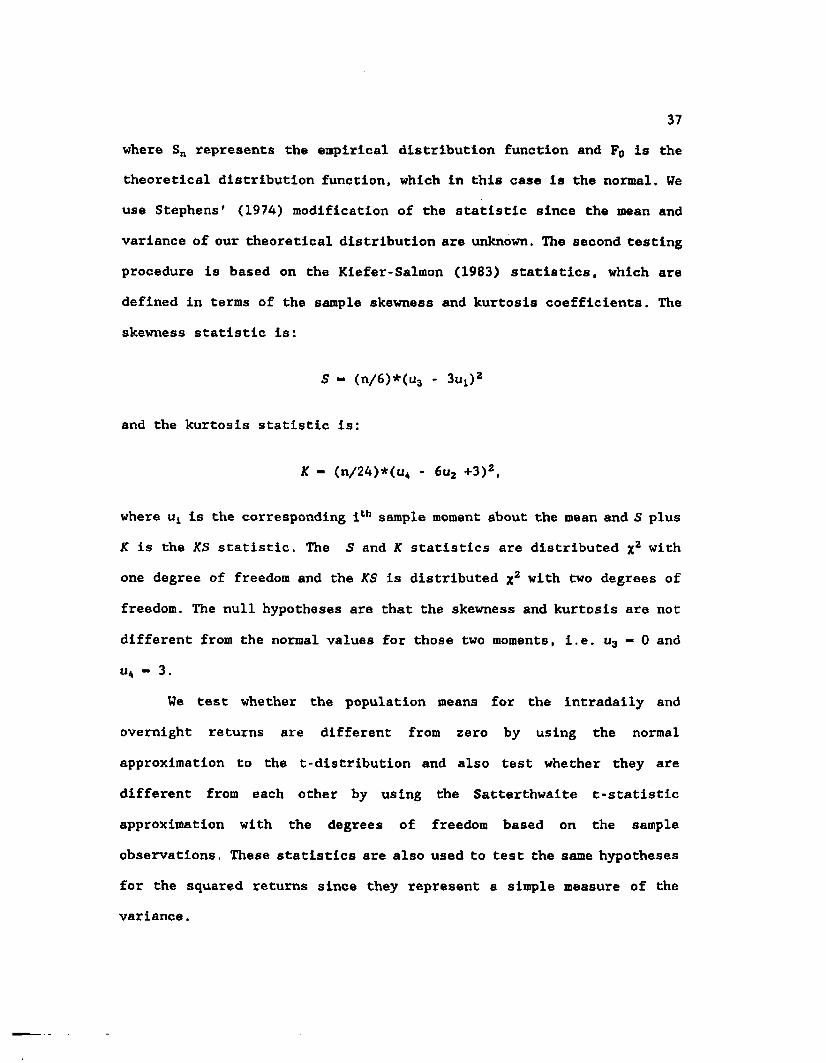
37where Sn represents the empirical distribution function and F0 is the theoretical distribution function, which in this case is the normal. We
use Stephens' (1974) modification of the statistic since the mean and
variance of our theoretical distribution are unknown. The second testing
procedure is based on the Kiefer-Salmon (1983) statistics, which are defined in terms of the sample skewness and kurtosis coefficients. The skewness statistic is:
S - (n/6)*(u3 - 3ut)2
and the kurtosis statistic is:
K - (n/24)*(u* - 6u2 +3)2,
where Ui is the corresponding 1th sample moment about the mean and S plus
K is the KS statistic. The S and K statistics are distributed %2 with
one degree of freedom and the KS is distributed x2 with two degrees of
freedom. The null hypotheses are that the skewness and kurtosis are not
different from the normal values for those two moments, i.e. u3 - 0 and
u* - 3.
We test whether the population means for the intradaily and
overnight returns are different from zero by using the normal
approximation to the t-distribution and also test whether they are
different from each other by using the Satterthwaite t-statistic
approximation with the degrees of freedom based on the sample
observations. These statistics are also used to test the same hypotheses
for the squared returns since they represent a simple measure of the variance.

38The next set of statistics deal with the null hypothesis of strict
white noise for the original return series and the presence of dependency in the squared and absolute return series. This set includes
Fisher's kappa and Bartlett's Kolmogorov-Smirnov statistics, which both test the null of strict white noise for the original returns in the time
domain. The Box-Pierce portmanteau test with modifications by Ljung and
Box (1978) is used to test for the above hypothesis in the frequency
domain16 and also to determine the presence of any nonlinear dependency
when applied to the squared and absolute return series.17 The general form of the Ljung-Box portmanteau Q statistic is:
Q - n(n+2) £ r ^ D A n - i ) ,
where n is the number of observations, r(i) is the autocorrelation
coefficient with a lag of i, and M is the maximum number of lags. The
statistic is distributed as a xz(M-p-q) where p is the order of the
autoregressive component and q is the order of the moving average. The
null hypothesis is that the series is a white noise process.
16 Fuller (1976) has a description of the two time domain tests on pages 282-287. Both are based on an analysis of the periodogram which Is generally used to search for cycles in the data. Fisher's kappa uses the largest periodogram, while Bartlett's is based on the normalized cumulative periodogram. The null hypothesis for Fisher's kappa is:Xt - u + et (white noise) versus Xt - u + Acosot + Bslnot + et, where o is unknown.
17 A discussion of the application of this statistic to the squared residuals can be found in McLeod and Li (1983). Another statistic used to test for nonlinear dependence is the TR2 statistic, a variant of the Lagrange multiplier test under asymptotic normality.

39The final statistic used is a Pearson %z goodness of fit test. This
is defined as:
kQk-i “ 2 ( y t - n P i o ) V n P l0»i-i
where k is the number of mutually exclusive cells into which the data
are subdivided, Pio is the theoretical probability of an observation
occurring in that cell, n is the number of observations, and yt is the standardized returns,18
Kendall and Stuart (1977, p. 463) argue that the best way to determine the class boundaries is to use an equal probabilities method
where Pio is equal to 1/k. In order to determine the number of classes they provide the following formula:
k - bl 2w(n-l)/(l, + G_1[P0]) )2/s
where b is between 2 and 4, n is the sample size, a is the size of the
test, la is the upper a-percentage point of the standard normal
distribution, P0 is the approximate power function for the maximization,
and G'1 is the inverse of the standard normal distribution function. The
statistic Ok-! is distributed as x2(k-l-m), where m is the number of
estimated parameters. He use this x2 test to determine the model that
best fits the empirically determined conditional distribution, which is
based on the estimated degrees of freedom.
18 The yt may also represent the standardized residuals when the procedure is used to test the fit of each model.

40C. DISCUSSION AND RESULTS
1. Ten minute data
We begin our analysis by examining the descriptive statistics for the ten minute data. From Table 3-2, we first notice the wide range of
values for the mean returns. For instance, DOW has a mean return of .00009641 which translates into an 8.09X monthly return and an 96.3X
yearly return. On the other hand, GM experienced a ten minute average
return of -.00007355 which becomes a -6.17X monthly return and a -73.5% yearly return. Seven of the stocks have a negative average return, while
eight are positive. The standard deviations of the returns range from a
high of 0.5339 for PAC to a low of 0.2245 for ATL.The median return for all the stocks Is zero, while the values for
the interquartile range indicate a large dispersion for some of the stocks, such as PAC, and almost none in the case of BAX. In terms of skewness, six of the stocks have a negative value indicating the
distribution is skewed to the left with the highest being GM and nine
have a positive value indicating a longer tail to the right with the
highest in this case being RJR. All the stocks exhibit leptokurtosis or
thick-tails which is consistent with previous work on stock prices, whether daily or intradaily.
In terms of the tests for normality, we turn to Table 3-3. All of the samples reject normality using the Kolomogorov D-statistic, which is
not suprising given the nature of the test as a goodness-of-fit test
based on the empirical distribution function. We further examine this
issue by looking at the Kiefer-Salmon statistics for skewness and

41kurtosis. In terms of skewness, the high value of the S statistic for ten of the stocks leads to the rejection of the null hypothesis of a
zero third moment or a symmetric distribution. The K statistic for normal kurtosis rejects the null hypothesis in all but one case, which
is the same result as the combined KS statistic. Hence, any assumption
of a normal unconditional distribution can be thoroughly rejected for all of the stocks except PAC, where the evidence for rejection in not quite as strong. Since rejection of the normality hypothesis does not
indicate whether the returns are simply independent white noise
processes, we examine the values for Fisher's kappa (K) and Bartlett's
(B) statistic. Using Fisher's kappa statistic we would reject the null
hypothesis of white noise for only two of the stocks, while Bartlett's test rejects the null for eleven out of the fifteen stocks.
Our next table, Table 3-4, provides the results of several tests for an end of day effect in both the mean and variance. The first two
columns give the results for the test that the means for the intraday
and end of day returns are significantly different from zero. We cannot
reject the null hypothesis of a zero mean intraday return for any of the
stocks in our sample, but we can reject the null for the end of day
returns in eight of our fifteen companies. These companies also exhibit
a statistical difference between the means of the two periods, thereby
providing some evidence for a mixture of distributions model based on
different means. However, as can be seen from the table, there is very
strong evidence that the major difference between these two periods is
in the variance. The results of these tests Indicate rejection of the
null hypotheses in all cases. Hence, there is very strong evidence of a

42non-stationary unconditional variance in the return series for the entire sample and an indication that standard estimation techniques are not appropriate.
In Table 3-5, we examine the degree of autocorrelation in the mean
while also checking for non-linear dependence, or dependence in the
variance. To accomplish this, we use the Ljung-Box statistics on the original returns r, the squared returns r2, and the absolute returns I rl .
The results for the original return series are in agreement with
Bartlett's test, rejecting the null hypothesis of strict white noise in
eleven out of the fifteen stocks. Hence, at least in terms of the actual
return series, out of our sample of fifteen stocks, only DIG, DOW, PHI,
and RJR exhibit a re turn-generating process that cannot be distinguished from a white noise process or one with no first order dependency.
We next turn to an examination of the degree of higher order
dependency, in particular second-order. Since our previous tests
indicated that the intradaily mean is not statistically different from
zero, we use the sum of squared returns as an approximation for the
variance. The results for the squared returns indicate that only in the
case of DIG and PHI can we not reject the null hypothesis. This finding
agrees with the lag-1 autocorrelation results in both the return and
squared return series. In the case of the absolute returns, all of the
stocks show a significant level of dependence in both tests. Hence, our
results for the ten minute data indicate that a model capable of
incorporating both linear and non-linear dependence is required.

432. Thirty minute data
We now turn to an examination of the thirty minute results. Generally it has been found that as the interval length over which
returns are estimated is lengthened, the degree of autocorrelation and
departures from normality exhibited by the data are reduced, tfe find the
same effect for this group of stocks. For example, in looking at Table
3-6, we see that the degree of kurtosis for all but three stocks is
reduced as we move from ten minute to thirty minute intervals. The same
holds true when we look at the actual hypothesis tests for normality
found in Table 3-7. For instance, the number of stocks for which the
null hypothesis of zero skewness can be rejected drops from ten to six.
Also Fisher's kappa statistic leads to a rejection of the white noise
hypothesis in only one of the fifteen stocks and Bartlett's test rejects
the null in six of the samples. However, the other tests for normality,
the D-statistic and the K and KS statistics reject the null in all the
cases. Hence, even at thirty minute intervals, the leptokurtosis in the
return series is very evident. Also a quick check of the ratio of the
variances between the ten and thirty minute intervals indicate that the
thirty minute interval variances are only roughly twice as large as the
ten minute ones, thereby rejecting not only the normality assumption but
also that of a random walk.19
19 In order for the random walk hypothesis to be accepted the ratio must be around three. This concept will be further discussed in Chapter 6 .

44We next turn to Table 3-8 where we have the mean and variance
effects based on the end of day dummy. We see that aggregation of the data has reduced the significance of the mean in distinguishing between
the two periods. Only two of the stocks, DOW and RJR, exhibit any
difference between the periods. On the other hand, the variance effect
still exists in twelve of the fifteen stocks.
This leads to the tests for nonlinear dependence in Table 3-9. In
terms of the original return series, we see from the Ljung-Box (LB) test
that first order dependence is exhibited in only four of the stocks, but
second order dependence, based on the results of the squared and
absolute returns, remains strong in eleven of the stocks. The lag-1 autocorrelation results provide similar evidence with an indication that
one period mean lags remain significant in eight of the cases and twelve
of the stocks exhibit higher order dependence for at least lag-1.
In conclusion, the results of this chapter Indicate that intraday
returns exhibit not only first order dependence, as documented by
previous authors, but also second order dependence. We also find that
evidence exists to confirm both the finding of a non-stationary
unconditional variance and a mixture of distributions hypothesis.
However, because of the presence of higher order dependence, we conclude
that any model of the return generating process for intradaily returns
that assumes independence is inappropriate. We therefore examine in the
next chapter a method for dealing with this problem.

45TABLE 3-1
LIST OF COMPAMIES
AME American Express
ATL Atlantic Richfield
ATT American Telephone and TelegraphBAX Baxter TravenolBOE Boeing
CHE Chevron
DIG Digital EquipmentDOW Dow Chemical
GE General ElectricGM General MotorsITT International Telephone and Telegraph
MOB MobilFAC Pacific Gas & ElectricPHI Phillips PetroleumRJR RJR Nabisco

46TABLE 3-2
TEN MINUTE DATA DESCRIPTIVE STATISTICS
mean(0000)
std dev (00)
skew kurt med IQR(00)
AME .1841 .4280 .4273 2.937 0.00 0.677
ATL -.0144 .2245 .2488 3.681 0.00 0.273ATT .4801 . 3349 .0476 0.969 0.00 0.722BAX .8356 .4100 .4867 2.635 0.00 0.000BOE -.2386 .2784 -.1228 3.028 0.00 0.487CHE -.6467 .3059 .2026 1.086 0.00 0.460
DIG .2512 .2397 .5763 3.827 0.00 0.263
DOW .9641 .2792 .0782 2.606 0.00 0.255
GE -.0219 .3398 -.1861 5.000 0.00 0.408
GM -.7355 .2377 -.3655 7.231 0.00 0.288
ITT .1510 .2323 -.0399 3.767 0.00 0.398
MOB -.4289 .3392 -.1801 4.746 0.00 0.501
PAC -.4133 .5339 -.1027 0.245 0.00 1.231
PHI .4258 .2944 .9781 8.840 0.00 0.224
RJR .1402 .3634 1.1636 8.843 0.00 0.379

47TABLE 3-3
TEH MINUTE DATATESTS FOR NORMALITY AND WHITE NOISE PROCESSES
Dstat
Sstat
Kstat
KSstat
K B
AME .1905* 27.88* 325.20* 353.08* 6.033 .1270*
ATL .1907* 9.45* 511.46* 520.91* 6.217 .0738ATT .2424* 0.35 35.07* 35.42* 6.490 .1368*
BAX .2611* 36.17* 261.78* 297.95* 6.360 .1154*BOE .2017* 2.30 345.77* 348.08* 7.802 .1602*
CHE .1782* 6.26* 44.18* 50.44* 6.712 .1072*
DIG .1081* 50.71* 552.83* 603.54* 5.813 .0356
DOW .1275* 0.93 255.92* 256.85* 6.595 .0348
GE .1646* 5.29* 944.50* 949.79* 6.351 .0773*
GM .1732* 20.39* 1977.33* 1997.72* 5.087 .0896*
ITT .2110* 0.24 535.67* 535.91* 7.680 .0910*
MOB .2044* 4.95* 850.96* 855.91* 5.420 .0929*
PAC .2376* 1.61 2.15 3.76 11.025* .2478*
PHI .1257* 146.06* 2955.53* 3101.59* 6.938 .0595
RJR .1609* 206.71* 2957.92* 3164.63* 9.165* .0454
The critical values for the D-statistic at the 0.10, 0.05, and 0.01 significance level are .0270, .0295, and .0341 respectively. The X2(l) value for the S and K statistics at the 0.05 significance level is 3.84. The %z(2) value for the KS statistic is 5.99 at the 0.05 significance level. Fisher's kappa critical values are 8.302, 9.006, and 10.600, while Bartlett's test statistic has 0.05 and 0.01 critical values of .06418 and .07692 (An represents significance at the 51 level.)

48TABLE 3-4
TEN MINUTE DATATESTS FOR UNCONDITIONAL MEAN AND VARIANCE EFFECTS
MEAN EFFECT VARIANCE EFFECT
H0: Pi - 0 H0: Pi“P2 H„: Pi - 0 H0: Pi-p2
means of returns means of variances(0 0 0 ) (0 0 0 0 )
0 1 0 1
AME -.097 1.51 0.144 0.682(0.67) (2.89)* (8.76)* (11.02)* (14.50)* (121.12)*
ATL -.032 0.40 0.046 0.107(0.42} (1.63) (2.28) (11.22)* ( 7.30)* ( 15.93)*
ATT - . 0 0 0 0.67 0.098 0.299(0.00) (1.64) (2.49) (15,25)* (13.04)* ( 71.68)*
BAX -.006 1.25 0.148 0.419(0.05) (2.48)* (5.78)* (12.17)* ( 9.59)* ( 35.62)*
BOE -.046 0.27 0.065 0.238(0.49) (0.75) (0.78) (11.40)* (11.55)* ( 65.23)*
CHE -.079 0 . 1 2 0.089 0.141(0.76) (0.33) (0.27) (16.03)* ( 7.03)* ( 6.11)*
DIG -.045 0.94 0.049 0.161(0.56) (3.19)* (10.40)* (10.72)* ( 9.66)* ( 41.79)*
DOW 0.063 0.53 0.067 0.223(0.66) (1.54) (1.72) (11.91)* (11.17)* ( 57.28)*
GE - . 1 0 2 1.29 0.096 0.366(0.89) (3.10)* (10.41)* ( 9.40)* (10.03)* ( 50.87)*
GM -.109 0.39 0.050 0.142(1.35) (1.35) (2.78) ( 8.60)* ( 6.81)* ( 18.13)*
ITT -.062 1 . 0 2 0.42 0 . 2 0 1
(0.79) (3.58)* (13.42)* (10.12)* (13.33)* (102.64)*MOB -.113 0.87 0.092 0.416
(0.98) (2.08)* (5.14)* ( 9.35)* (11.82)* ( 78.63)*PAC -.044 Oo1 0.272 0.451
(0.24) (0.00) (0.00) (18.75)* ( 8.64)* ( 10.93)*PHI -.039 1 . 1 0 0.065 0.360
(0.39) (3.05)* (9.24)* ( 6.96)* (10.62)* ( 70.37)*RJR -.138 1.98 0.092 0.650
(1.12) (4.48)* (21.31)* ( 6.56)* (12.90)* (113.93)*
The corresponding t-statlstics for the null hypotheses are presented in parentheses. The 0 columns represent the intraday results and the 1 columns the end of day results. (An representssignificance at the 5% level.)

49TABLE 3-5
TEN MINUTE DATATESTS FOR NONLINEAR DEPENDENCE
LB(6 )r
LB(6 )r2
LB(6 )Irl
AUTOCORRELATION FOR r r2
LAG-1 1 rl
AME 35.71* 22.53* 49.14* -.1878* .1115* .1537*ATL 16.76* 82.32* 104.15* -.0696* .1866* .2175*ATT 51.95* 19.40* 21.76* -.1908* .1270* .1129*
BAX 28.06* 14.29* 30.45* -.1700* .0663* .1257*BOE 49.87* 50.85* 71.22* -.2241* .0817* .0814*
CHE 32.26* 63.51* 33.66* -.1478* .1560* .1050*DIG 8.18 7.28 50.60* -.0320 .0268 .0978*
DOW 5.02 89.06* 100.34* .0309 .2154* .2462*
GE 14.83* 172.15* 133.29* -.0906* .3598* .2764*
GM 17.51* 218.47* 199.81* -.1065* .3725* .2931*
ITT 20.07* 14.89* 20.82* -.1342* .1209* .1293*
MOB 20.82* 98.28* 106.28* -.1106* .1643* .2 1 0 0 *
PAC 146.08* 20.81* 16.87* -.3894* .0884* .0944*
PHI 10.89 9.56 82.99* -.0676* .0277* .1310*
RJR 10.24 27.68* 61.74* .0255 .1439* .1585*
The critical values for the Ljung-Box, LB(6 ), statistic at the 0.10, 0.05, and 0.01 significance level are 10.64, 12.59, and 16.81 respectively, (An '*' represents significance at the 5% level.)

50TABLE 3-6
THIRTY MINUTE DATA DESCRIPTIVE STATISTICS
mean(0 0 0 0 )
std dev (0 0 )
skew kurt med IQR(0 0 )
AME .5272 .6567 .2256 1.454 0 . 0 0 0.691
ATL -.0413 .3629 .0920 3.238 0 . 0 0 0.283
ATT 1.3746 .4982 .1944 1 . 2 2 0 0 . 0 0 0.741
BAX 2.3922 .6470 .2489 1.977 0 . 0 0 0.889BOE -.6831 .3885 -.3112 2.025 0 . 0 0 0.493CHE -1.8513 .4693 .3902 1.546 0 . 0 0 0.471DIG .7192 .4042 .1095 1.653 0 . 0 0 0.458
DOW 2.7602 .5028 -.0839 4.637 0 . 0 0 0.505GE -.0626 .5408 -.3308 2.740 0 . 0 0 0.419GM -2.1058 .3704 -1.0767 5.237 0 . 0 0 0.300ITT .4322 .3513 -.1288 2.143 0 . 0 0 0.403
MOB -.1228 .4913 .1268 1.296 0 . 0 0 0.515
PAC -1.1831 .5886 -.2705 0.667 0 . 0 0 1.242
PHI 1.2190 .4756 .5377 3.496 0 . 0 0 0.439
RJR .4015 .5670 .8209 3.767 0 . 0 0 0.737

51TABLE 3-7
THIRTY MINUTE DATATESTS FOR NORMALITY AND WHITE NOISE PROCESSES
Dstat
Sstat
Kstat
KSstat
K B
AME .1325* 2.70 26.69* 29.39* 4.334 .1732*
ATL .1348* 0.45 134.38* 134.83* 4.611 .1036ATT .1933* 2 . 0 0 18.69* 20.69* 5.342 .1159*BAX .1908* 3.28 49.73* 53.01* 4.053 .1190*B0E .1736* 5.13* 52.18* 57.32* 3.958 .1272*CHE .1152* 8.07* 30.19* 38.26* 6.322 .1455*DIG .0915* 0.63 34.62* 35.25* 9.240* .0928DOW .1 0 1 1 * 0.37 276.53* 276.90* 5.143 .0684
GE .1 1 2 0 * 5.80* 95.97* 101.77* 4.217 .0586GM .1349* 61.44* 353.06* 414.50* 4.304 .0684ITT .1496* 0 . 8 8 58.49* 59.37* 4.934 .0603
MOB .1348* 0,85 21.15* 2 2 .0 0 * 4.412 .0844
PAC .2245* 3.88 5.44* 9.32* 5.755 .1583*
PHI .1072* 15.32* 156.72* 172.04* 5.670 .0496
RJR .1227* 35.71* 182.12* 217.83* 4.371 .0748
The critical values for the D-statistic at the 0 .1 0 , 0.05, and0.01 significance level are .0456, .0498, and .0576 respecCively. The X2 (l) value for the 5 and K statistics at the 0.05 significance level is 3.84. The x2 (2) value for the KS statistic is 5.99 at the 0.05 significance level. Fisher's kappa critical values are 7.230, 7.895, and 9.439, while Bartlett's test statistic has 0,05 and 0.01 critical values of .10785 and .12927 (An '*' represents significance at the 5Z level.)

52TABLE 3-8
THIRTY MINUTE DATATESTS FOR UNCONDITIONAL MEAN AND VARIANCE EFFECTS
MEAN EFFECT VARIANCE EFFECT
H0: Pi - 0 H0: Pi-p2 H0: Pi - 0 H0: Pi-p2
means of returns means of variances(0 0 0 ) (0 0 0 0 )
0 1 0 1
AME -.138 0.79 0.326 0.833(0.33) (0.97) (1.0*) ( 6.7*)* ( 8.77)* ( 22.69)*
ATL .003 - . 0 0 0.115 0.193(0.01) (0.69) (0.00) ( 6.20)* ( 5.27)* ( 3.57)
ATT .089 0.32 0 . 2 2 2 0.346(0.28) (0.53) (0.12) ( 8.0*)* ( 6.38)* ( 4.17)*
BAX .107 0.75 0.334 0.743(0.26) (0.9*) (0.51) ( 6.52)* { 7.39)* ( 13.15)*
B0E -.058 - . 1 1 0.118 0.274(0.2*) (0.23) (0.01) ( 6.*0)* ( 7.56)* { 14.63)*
CHE -.053 -.69 0.203 0.285(0.18) (1.20) (0.98) ( 7.96)* ( 5.68)* ( 2.15)
DIG -.156 0.95 0.129 0.296(0.62) (1.92) (3.97)* ( 6.77)* ( 7.93)* ( 15.93)*
DOW 0.339 0.03 0.186 0.511(1.07) (0.05) (0.19) ( *.70)* ( 6.56)* ( 13.83)*
GE -.140 0.51 0.224 0.552(0.*1) (0.77) (0.76) ( 5.79)* ( 7.26)* ( 14.79)*
GM -.173 - .36 0.115 0.223(0.7*) (0.78) (0.13) ( 4.96)* ( 4.88)* ( *.*0)*
ITT -.011 0.25 0.092 0.244(0.05) (0.58) (0.30) ( 6.07)* ( 8.23)* ( 20.95)*
MOB -.203 0.19 0.190 0.437(0.66) (0.31) (0.33) ( 7.17)* ( 8.38)* ( 17.80)*
PAC -.051 -.38 0.322 0.435(0.1*) (0.52) (0.16) ( 9.13)* ( 6.27)* ( 2.08)
PHI -.062 0.83 0.172 0.432(0.21) (l.*2) (1.86) ( 5.30)* ( 6.77)* ( 13.18)*
RJR -.303 1.36 0.233 0.660(0.86) (1.97)* (*.59)* ( *.96)* ( 7.15)* ( 17.06)*
The corresponding t-statistics for Che null hypotheses are presented In parentheses. The 0 columns represent the intraday results and the 1 columns the end of day results. (An representssignificance at the 5X level.)

53
TESTS
TABLE 3-9 THIRTY MINUTE FOR NONLINEAR
DATADEPENDENCE
LB<6 )r
LB(6 )r2
LB(6 )Irl
AUTOCORRELATION FOR r r2
LAG-11 rl
AME 2 0 .1 2 * 19.13* 30.92* - .2063* .2123* .2762*ATL 10.04 28.69* 37.64* -.1326* .2062* .2351*ATT 8.52 14.34* 5.46 -.1310* .0679* .0687
BAX 10.39 10.13 19.85* -.1416* .1676* .2134*BOE 12.47 23.31* 24.83* -.1680* .2042* .2144*CHE 39.12* 34.59* 31.52* -.1910* .1802* .2650*
DIG 7.09 14.24* 16.90* -.0356 .1405* .1081*
DOW 4.55 13.33* 35.02* .0484 .1811* .2600*GE 6.34 23.83* 23.46* -.0545 .2087* .1253*
GM 7.05 20.55* 11.18 -.0667 .1 0 0 2 * .0933
ITT 3.67 5.91 5.89 -.0768 .0863 .0914
MOB 9.58 19.88* 22.92* -.0732 .1874* .1845*
PAC 17.08* 8 . 2 2 4.31 -.1935* .0343 -.0023
PHI 2.72 5.10 11.17 -.0298 .1078 .1513*
RJR 11.28* 1.80 4.92 -.0644* .0237 .0448
The critical values for the Ljung-Box, LB(6 )f statistic at the 0,10, 0.05, and 0.01 significance level are 10.64, 12.59, and 16.81 respectively. (An '*' represents significance at the 5% level.)

CHAPTER 4MODEL ESTIMATION
The finding of non-linear dependence in intradaily returns requires us to use a more general class of processes than standard
linear time-series models, such as the autoregressive moving average
(ARMA) processes of Box-Jenkins. It also rules out a number of processes used previously in the literature to model security returns, such as the
Stable-Paretian, Student-t, and mixture of normals.
Priestley (1980) offers a general state dependent approach for
handling non-linearities that includes the bilinear model of Granger and Anderson (1978) and the exponential autoregressive model of Haggan and
Osaki (1981). We choose to employ a variant of the bilinear processes known as the autoregressive conditional heteroskedasticity (ARCH) model, since its estimation techiques are well developed. Also, the ARCH model
has been proven suitable for modelling the time series properties of
returns for longer sampling intervals, such as a day or week.
In the first section of this chapter, we introduce the theory
behind both the ARCH model and the more general GARCH model. In the
second section, we discuss the specific formulations and rationale for
using the conditional distributions, which include the normal, Student-
t, and power-exponential. We also introduce the particular classes of
ARCH and GARCH and the criterion we use for selecting the model that
best fits the data. In the final section, we present our results and a
discussion of their implications for the return generating process of stock returns.
54

A. ECONOMETRIC THEORY55
Engle (1982) first Introduces the ARCH model as a means fordealing with a non-stationary variance and second order dependency. He specifically expresses the conditional variance as a function of past
values of the random variable. He points out that the conditional means
and variances may evolve jointly over time, thereby requiring
simultaneous estimation. His ARCH(q) model has the following form:
rtJ *t-i “ N(xtB,ht)
ht - *o + E ai«g-i i-l
et - rt - xtB,
where ¥t-i is the information set at time t-1 , xt is the vector of
independent variables, the a's and B's are vectors of unknown parameterswith a0 > 0 and a* i 0, and ht is the variance of the errors. The
conditional distribution of rfc, or rtl ¥fi» an(* et are assumed to be normal.
Engel makes a number of comments concerning the specification of
the conditional variance or ht. First, he notes that large observations,
in absolute value, will lead to a larger variance for next period's
distribution. Secondly, if the coefficient of the squared lag value is
positive, i.e. aA > 0 , then successive observations are dependent through
higher moments. Thirdly, the first order process will generate fatter
tails for the unconditonal distribution than the normal. And lastly, the temporal clustering of outliers may be used to predict their occurrence.
The first and third comments arise from the expressions for the
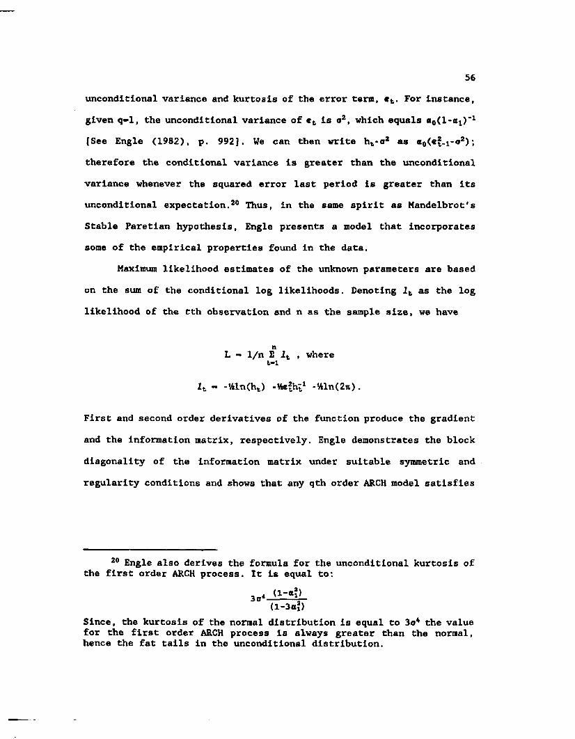
56unconditional variance and kurtosis of the error term, «t. For instance,
given q-1 , the unconditional variance of et is a2, which equals SoCl* * ] . ) " 1
[See Engle (1982), p. 992]. We can then write ht-o2 as «0 (e|.1 -o2);
therefore the conditional variance is greater than the unconditional
variance whenever the squared error last period is greater than its unconditional expectation. 2 0 Thus, in the same spirit as Mandelbrot's
Stable Paretian hypothesis, Engle presents a model that incorporates
some of the empirical properties found in the data.
Maximum likelihood estimates of the unknown parameters are based
on the sum of the conditional log likelihoods. Denoting lt as the log
likelihood of the tth observation and n as the sample size, we have
nL - 1/n £ It , wheret-i
lt - -%ln(ht) -lAefrt1 -ttln(2 *) .
First and second order derivatives of the function produce the gradient
and the information matrix, respectively. Engle demonstrates the block
diagonality of the information matrix under suitable symmetric and
regularity conditions and shows that any qth order ARCH model satisfies
2 0 Engle also derives the formula for the unconditional kurtosis of the first order ARCH process. It is equal to:
— ——It—(l-3aj)Since, the kurtosis of the normal distribution is equal to 3o* the value for the first order ARCH process is always greater than the normal, hence the fat tails in the unconditional distribution.

57the regularity conditions if a0 is greater than zero and the a^'s are greater than or equal to zero. 2 1
Ve use an iterative estimation procedure based on the algorithm of fierndt, Hall, Hall, and Hausman (1974) to obtain the maximum likelihood
estimates of the a's and B's. This algorithm provides a numerical
solution for the first derivatives of the likelihood function with the iterations for the s's and B's being carried out separately because of
the block diagonality of the information matrix. Each step produces
parameter estimates 0 i + 1 based on the preceding estimates according to
el+1 - e1 + xL ( s t o i t / a e j o i t / a e')]!-1 I ait/aot-i t-i
where the 3It/30 is evaluated at fl1, the parameter estimates for the ifch step, and the li is the step length. Three convergence criterion are
used. The first is based on the gradient around the inverse of the
Hessian matrix, which can be interpreted as the remainder of a Taylor
series expansion around the estimated maximum. The second is the change
in the calculated log likelihood function and the third is the change in
the gradient for each iteration. Weiss (1986) demonstrates the
consistency and aysmptotic normality of the maximum likelihood
estimates. Hence, standard t-statistics are used to test whether the
parameters are significantly different from zero.
2 1 Proofs of these theorems can be found in the appendix of Engle (1982).

58Bollerslev (1986) respeclfies the ARCH process in terras of a
generalized autoregressive conditional heteroskedasticity or GARCH
model. He points out that most applications of ARCH have used a linear lag structure, while GARCH will allow for a more flexible one. In the
same manner that the ARMA model is a generalization of the AR model for
the mean or first moment, so is the GARCH a generalization of ARCH for
the variance or second moment. Hence, just as the autocorrelation and
partial autocorrelation functions are useful in identifying and checking
the times series behavior of the ARMA process for the conditional mean,
the same procedure can be used on the squared process for checking and
identifying GARCH behavior In the conditional variance. Whereas the ARCH process specifies the conditional variance as a linear function of past
sample variances only, the GARCH(p.q) process includes lagged
conditional variances as well. Hence, this allows for the possibility of
an adaptive learning mechanism based on the past conditional variances.
Bollerslev1s generalized autoregressive conditional
heteroskedasticity (GARCH) model has a conditional variance equation of:
i , p hfc - «„ + E ajef-i +E Pih^,i-l 1 - 1
where pzO, q>0, a0>0, a^O, and PizO. He notes that for 'p-0 the process
reduces to the ARCH(q) process, and for p—q—0 et is simply white q p
noise. ' 2 2 When Ea* + Ep. < 1 the process is considered stationary and l-i 1 - 1
the unconditional variance of the et's is defined as ^/(l-Es^Ep^ [See
Bollerslev (1986)]. Maximum likelihood estimates of the regression
2 2 Bollerslev (1986), p.309.

59parameters for both the mean and variance equations are obtained using the same iterative procedure outlined above for the ARCH model.
Bollerslev's (1987) second contribution concerned the
specification of the conditional density. By allowing for t-distributed
conditional errors, he points out that this 'permits a distinction
between conditional heteroskedasticity and a conditional leptokurtic
distribution, either of which could account for the observed
unconditional kurtosis in the data. ' 2 3 This distinction plays an
important role in the model's ability to fit the observed data, a point
we will discuss further in the following section.
B. HODEL SPECIFICATION
Since part of our work concerns the differences that existence in
the returns based on ten and thirty minute sampling intervals, we employ four basic estimation models with three different conditional
distributions. Our first model assumes that there is no nonlinear
dependence while still retaining the linear dependency through the use
of a moving average process of order one, denoted MA(1). This is
consistent with the findings in Chapter 3, where some of the thirty minute returns exhibited little evidence of higher order dependency. The
three remaining models all take account of the nonlinear dependence and
are denoted as an ARCH(l), ARCH(2), and a GARCH(l.l) process respectively.
2 3 Bollerslev (1987), p.542.
In the same manner, we include three conditional distributions to account for the moment structure of the ten and thirty minute return series. These are the normal, Student-t, and power-exponential distributions. Uithin each model, we first estimate the parameters based
on the assumption of conditional normality. This is the original specification of the ARCH process developed by Engle. The formula for
the normal conditional density is:
N(et,ht) - (2*htr-5 exp[ -.5(e?)/ht].
The second specification of the conditional density is the
Student-t with reference to Bollerslev (1987). The conditional density is defined as:
T(et,htIdf) - rikl-rfdf/2]-1- [(df-2 )htp 3- [l+e?/(ht<df-2 ))]-k,
where F[ - ] is the gamma function, df are the degrees of freedom with the
restriction that they be greater than two, and k-(df+l)/2. Note that as
l/df-0 the t-distribution approaches the normal, Connolly (1989)
suggests that for df>30 and «lt Pi>0, time-varying heteroskedasticity
explains the leptokurtosis, while if df<1 0 , then both non-normality and
time-varying heteroskedasticity are possible explanations. However, this
observation seems to be more a rule of thumb rather than based on any statistical theory, since traditionally the Student-t is assumed to
approach normality at approximately 30 degrees of freedom.

61The third distributional assumption we use results from Nelson's
(1989) extension of the GARCH model with a conditional density based on
the Generalized Error Distribution (GED) or the power-exponential (PE) distribution as defined by Box and Tiao (1973). Its distributional form is:
PE(et ,ht ,df) - .5df-[r(3/df)]-5- ( r a / d f ) ] - 1-3-^ -
e x p { - [ I W d f ) / r ( l / d f ) ] " ' 2-l et/htl « ) ,
where df are the degrees of freedom. If df-2 we have the normal distribution, while df-1 gives us the double exponential. Box and Tiao
(1973) note that (2/df)-l gives a measure of kurtosis.
Figure 4-1 provides a graphical representation of the differences
between these three distributions. There are several important points to note. The first is that where as the Student-t approaches the normal
from below, the power-exponential approaches it from above. Hence, in
reference to Fama's (1965a) discussion on the peakedness of his daily
data [see footnote 8 ], the power-exponential would seem a priori to
provide a better fit to daily data than the Student-t. By reversing our
inferences about aggregated daily returns approaching normality, we can
argue that intradaily returns should exhibit even greater peakedness
while still retaining the leptokurtosis. The second point is that the
power-exponential has a large part of its density at the mid-point of
the distribution. This is generally consistent with a large number of
returns at zero. In fact a comparison of the distributions in Figure 4-1
Indicates that the power-exponential with one degree of freedom has

62roughly 12.4% of Its distribution ± 0.05 standard deviations from the mean as compared to 7.4% for the normal, and 7.1% for the Student-t with 5 degrees of freedom. The last point concerns the distribution of the
tail regions. The Student-t distributions exhibit fatter tails than the
normal at approximately 1.7 standard deviations from the mean while the
power-exponential distributions cross over at about 2.3 standard deviations. Hence, both the Student-t and power-exponential
distributions are considered leptokurtotic with the extent depending on
their respective degrees of freedom. For the Student-t and the power-
exponential distributions the appropriate degrees of freedom are
estimated in the maximum likelihood algorithm.
In terms of the actual models we estimate, we retain the two dummy
variables discussed in Chapter 3 in both the mean and variance equation. As mentioned, one represents the component of the return (or conditional
variance) which results from the bid-ask spread and the other is an end
of day dummy. The mean equation also contains a moving average term to
account for the autocorrelation found in the mean. Our general mean
equation is denoted by:
rt - a0 + ajEOD + aaAD + aa®^ + et,
where the rt are the ten or thirty minute returns, a0 is the mean
intercept, GOD is the end of day dummy, AD is the ask dummy,
represents the moving average process, and <t are the residuals. The
conditional distributions of the residuals include the normal, Student-

63t, and power-exponential. This equation represents our basic model that we denote as MA in the ensuing tables.
The variance equation has three functional forms depending on the degree of the ARCH process. The first is the ARCH of order one denoted as AR(1):
ht “ #o + ■*" 02®“OD + P3AD
The second if the ARCH of order two denoted as AR(2) with the following specification:
ht - o0 + aje?., + «2®t- 2 + P2 eod + P3AD
And the last is the GARCH(1,1) denoted as G(l,l):
ht - a0 + + Pi t-i + P2EOD + P3AD
Since the actual estimation requires the testing of a number of
alternative models, likelihood ratio tests are used to determine which
nested model fits the data better. The simple MA process is nested
within the conditionally normal family, which is in turn nested within
either the Student-t or power-exponential distributions. As noted by
Akgiray (1989), the test statistic is defined as:
LR - -2lL(6n) - L{6.)),

64where 0 n and 6 a are the parameter estimates under the null and alternative hypothesis respectively and the L(*) are the corresponding maximum log-likelihood values. The statistic is asymptotically %2
distributed with the degrees of freedom equal to the difference between
the number of parameters under the alternative and null hypotheses [See Akgiray (1989), p. 6 8 ], Since the Student-t and power-exponential
distributions are estimated separately a different test is required to
determine the best model among them. 2 4 We choose the Pearson x2 goodness of fit test discussed in Chapter 3 since it provides a statistical
comparison of the theoretical distribution based on the estimated
parameters and the empirical distribution of the standardized residuals,
«t/ht or rt. We also examine the standardized residuals to determine how
well the final models have eliminated the first and second order dependencies found in the original data.
C. ESTIMATION RESULTS
1. Ten minute data
We begin our discussion with the ten minute data. Table 4-1
provides the log-likelihood values for the four models with the normally
distributed conditional errors. The underlined values indicate those
models with the highest log-likelihood based on the likelihood ratio
test. As can be seen in the table, the simple MA model never does better
2 4 McDonald and Newey (1988) show that the power-exponential and the Student-t are included in a more general family of distributions known as the generalized t or GT. This possibility will be pursued in future work.

65than Che ARCH models Indicating that higher order dependence is present in all the stocks. Table 4-2 has the corresponding x2 values. They
indicate that the normal distribution provides a poor fit for all the ten minute return series since in all cases the null hypothesis is
rejected at the .05 significance level.
We next turn to the Student- 1 distribution and the log-likelihood
and x2 values found in Tables 4-3 and 4-4 respectively. Again the
evidence suggests that higher order dependency can be found in the data since the MA model is superseded by the other three. The Student- 1
models also provide a better fit to the data than the normal in 43 of
the 60 cases, however we still find that the null hypothesis of a good
fit is rejected in all cases. Hence, even though the fat-tailed Student-
t distribution does better than the normal it still is unable to provide a very good fit to the data.
We then look at the results for the power-exponential. We again
find that the simple MA model is out performed by the other three. We
also find that the power-exponential begins to address the empirical
data a little better. However in only one case, DIG, are we unable to
reject the null hypothesis at the .05 level. We will address this issue
in more detail later after we have determined the best model out of the ones we have tested.
In order to determine the best model out of the twelve possible
cases, we first use the likelihood ratio test to determine the best
models for each conditional distribution. These results are found in
Table 4-7. The results are dominated by the GARCH(1,1) and ARCH(2)
model. Since the normal results are nested within both the Student-t and

66power-exponential we are able to directly compare the log-likelihoods to determine if the normal is better than the other two. The evidence
suggests that only PAC returns exhibit a conditionally normal distribution. This result confirms the normality tests of Table 3-3
since this is the only stock where the Kiefer-Salmon tests for normality
could not reject the null hypotheses. Because the estimation algorithm
does not use a procedure that allows joint estimation of the Student-t and power-exponential distributions, we turn to the x2 results to
determine the best model. Based on these results we find that in the
case of AME, ATT, BOE, ITT, and MOB the Student-t distribution out performs the power-exponential. In the other nine cases the power-
exponential is the better model.
Hence, up to this point, we have found that ten minute return data
exhibit non-linear dependency and in general conditional leptokurtosis.
The evidence also indicates that our assumption about the peakedness of
the data is confirmed in nine out of the fifteen stocks sampled.
However, we do not find strong evidence in support of a single
conditional distribution that is able to model the ten minute return
series. We next examine the estimation results for our fifteen stocks
based on the best models in Table 4-7.
Table 4-8 contains the parameter estimates for the mean and
variance equations. We first examine the mean equation. The two results that immediately stand out are the significant coefficients for the ask
dummy, a2, and the moving average dummy, a3. In all cases, these
parameters are significantly different from zero further documenting the
effect of the bid-ask spread on the observed returns for short time

67intervals. In fact, the sign of the coefficients are all in agreement with previous work, with the negative moving average coefficient lending credence to Roll's (1984) hypothesized result concerning the bid-ask
spread creating negative serial correlation in the observed returns. The results for the end of day dummy, alP are less definitive with nine of
the stocks showing no effect on the mean return and six showing an effect. These results are in general agreement with those of Table 3-4
where we looked at the effects of the end of day dummy on the
unconditional mean and variance. The indication is that there is an end
of day effect in the mean but it is not universal to all stocks. He next
examine the results for the variance equation.The first points of interest are the parameters for nonlinear
dependence given by alt a2, anc* Pi- All of these coefficients are
significantly different from zero except ax for ITT. In every case the
sums are always less than one, indicating a stationary process. In
general, the Student-t and normal models have lower measures of
persistence in the variance than the power-exponential results. However,
there seems to be no definitive pattern in the behavior. The results
indicate that ARCH effects do exist in the returns of ten minute intervals.
Further information is obtained by looking at the end of day, p3,
and ask, £*, parameters. Of particular interest is the fact that the end
of day parameters are all significantly different from zero. This is in
agreement with the results of Table 3-4 on the unconditional variances.
Hence, this evidence collaborates previous work by Harris (1989) and
Hood et. al. (1985) on the differences between end of day and intradaily

68returns. It also extends the literature by finding that the end of day effect is more likely to be found in the variance than in the mean. The ask dummy is less conclusive with six of the stocks showing
insignificant results. Hence, the bid-ask effect seems to be
predominately in the mean with some stocks exhibiting dependency in the conditional variance. The last column is Table 4-8 provides the
estimated degrees of freedom for the conditional distributions. The
power-exponential results indicate a high degree of peakedness, while
three of the other six stocks are very close to a conditionally normal distribution.
In our last two tables we check the distributional and time series
properties of the standardized residuals in order to determine (1 ) where
the models fail to fit the empirical conditional distributions and (2 ) whether the models eliminate the first and second order dependence in
the data. From Table 4-9 we see that the skewness in the data is not
significantly different from zero in ten out of the fifteen stocks based
on the S statistics. However, it may explain some of the high %z values
in those stocks where there is evidence of skewness, such as ITT and
RJR. Three of these stocks also exhibit a higher measure of skewness in the residuals than in the original data. 2 5 On the other hand, our
measures of kurtosis are all in agreement with the estimated models
since PAC is the only one with no evidence of leptokurtosis.
2 5 Hsieh (1989b) argues that the skewness and kurtosis of the standardized residuals should be smaller than those of the raw data if the coefficients of the mean equation are very small. A large increase in the absolute size of those two moments is then seen as evidence against the model.

In the last two columns of Table 4-9, we attempt to ascertain where the models fail to fit the empirical distributions. Since the
total x2 measure is a sum of k independent x2s each of degree one, we sum
the corresponding estimates of the x2 f°r the tail and mid-point regions
of the distributions, respectively. In eleven out of the fifteen
samples, we cannot reject the null hypothesis of an adequate fit in the
tail regions and in eight out of the fifteen we cannot reject the null in terms of adequate fit over the mid-region of the distribution. In
fact in seven out of the fifteen stocks, both the tail and mid-point
regions are in agreement with their respective null hypotheses. Hence,
the models for the ten minute intervals are doing a better job of
fitting both the leptokurtosis and the peakedness of the data then we
originally thought. This raises the possibility that a mixture of
distributions with non-linear dependence may in fact be the true underlying process generating the returns.
In Table 4-10, we find that the estimated models do a fairly good
job of eliminating the higher order dependence in the data. In nine of
the stocks no evidence remains for either first order or second order
dependence based on both the Ljung-Box test and lag- 1 autocorrelation
statistics. In two of the remaining six the only evidence for dependency
is in the absolute residuals and in two of the others there is
dependence only in the mean. Interestingly, this first order dependence arises in two out of the three stocks where no such dependence existed
in the original data. Hence, the use of a general moving average process
of order one for all of the stocks may be inappropriate.

70In conclusion, we find that the power-exponential conditional
distribution with a GARCH(l.l) process is the model that best fits the
ten minute return series for the majority of the stocks in our sample.
However, the evidence suggests that a more appropriate specification of
the process is a mixture of distributions based on a model capable of
incorporating nonlinear as well as linear dependence. We shall attempt
to address this issue in future research. We now turn to an examination of the thirty minute results.
2. Thirty minute data
Table 4-11 provides the log-likelihood values for the four models with normally distributed conditional errors. As opposed to the ten
minute results, the simple MA model does better than any of the ARCH
models for three of the stocks indicating that higher order dependence
may have been eliminated through the aggregation of the data. An
examination of Table 4-12 shows that the %2 values are generally lower
for the thirty minute returns than for the corresponding ten minute ones
but are not significant in only three of the possible cases.
The Student-t results in Tables 4-13 and 4-14 indicate that a
simple MA model fits several of the stocks better than any of the ARCH
models. The x2 tests indicate that the null hypothesis of a good fit is
rejected in every case for the Student-t models. However, the fit seems
to be better overall for the thirty minute data than the ten minute
data. The results for the power-exponential distribution are reported in
Tables 4-15 and 4-16. An additional stock, ATT, is added to the list of

71stocks where the simple MA model fits better than the ARCH models. Hence, there are very strong Indications that unconditionalleptokurtosis is a result of the conditional leptokurtosis and not of any heteroskedasticity in the data. We will examine this issue in more detail later. The %2 results in Table 4-16 indicate that the power-
exponential still holds the highest possibility for fitting the data
since nine of the cases cannot reject the null hypothesis concerning the
goodness of fit.
We next determine the best models for the data based on the
likelihood ratio test and the x2 goodness of fit results. Table 4-17
indicates that three of the fifteen thirty minute returns are best modelled as conditionally normal distributions. These are the returns
for AME, CHE, and PAC. If we look back at Table 3-7 we see that all
exhibited excess kurtosis, but only CHE rejected the null hypothesis of
no skewness. The evidence in Table 3-9 shows that nonlinear dependence
existed in the AME and CHE series but not in the PAC returns. This is in agreement with the estimated models since the first two are a GARCH(l.l)
and an ARCH(2) respectively, while the third is a simple MA.
Interestingly both AME and CHE had the lowest estimated degrees of
freedom for their respective models in the ten minute results while PAC
already exhibited normality. Therefore there is agreement between the
two time series in terms of the gradual move to normality as the returns
are aggregated. Also of note is that AME remained a GARCH(l.l), CHE
became an ARCH(2), and PAC a simple MA as we aggregated the results. So
there is a movement toward normality not only in the shape of the
distribution but also in the loss of nonlinear dependence.

72The Student-t distribution yields the best model for three stocks,
ATT, BAX, and ITT. The ten minute results for ATT indicated a GARCH(l.l), with the thirty minute results indicating an ARCH(2). It retained the general distributional shape while exhibiting less second order dependence. The BAX returns, on the other hand, flatten out from
a power-exponential to a Student-t while still keeping the estimated
GARCH(1,1) albeit lower in magnitude. Lastly, the ITT results indicate
the same general shape for both the ten and thirty minute intervals,
while losing their nonlinear dependence all together in the thirty
minute returns. Hence, the pattern developing is that each stock has its
own empirical characteristics with the aggregation leading to a
reduction in the nonlinear dependence and/or a shift toward conditional normality.
Nevertheless, as was found for the ten minute results, the power- exponential continues to provide the best fit, in this case for nine of the fifteen stocks. However, the results for two stocks, BOE and MOB,
are contrary to our previous observation. BOE goes from an ARCH(2) to an
ARCH(l) but actually becomes more peaked as it is aggregated. One
possible explanation for this behavior is that the high first order
negative autocorrelation in the mean for the ten minute data was
cancelling out in the larger returns and creating more returns close to
zero as they were aggregated. There seems to be no way to predict this
peculiar behavior and for now we simply document it as an idiosyncrasy
of that particular stock. In the case of MOB, not only do the returns
become more peaked but they also have a greater degree of nonlinear
dependence. However, the significance of that nonlinear dependence is

73called Into question by the fact that Its parameter estimate is not significantly different from zero. We discuss this further in the next
section. The remaining stocks all exhibit the same general behavior
mentioned previously. For instance ATL, GE, and CHE go from a GARCH(l.l)
to an ARCH(2) with the last stock becoming normal as noted above. Three
stocks, DIG, DOW, and RJR remained power'exponential GARCH(1,1) for both
return series, while GM and PHI went from a power-exponential GARCH(1,1) process to a power-exponential MA process.
We next examine the estimated parameters in Table 4-18 alluded to
briefly in the prior discussion of the MOB results. The first point of
interest is the lack of explanatory power for our two dummy variables in
the mean equation. In only two cases, DIG and GE, is coefficient for the
end of day dummy significantly different from zero at the .05 significance level and in none of the stocks is the ask dummy
coefficient significant. This last point is especially striking since
the coefficient for the same dummy was significantly different from zero
in every one of the stocks in the sample over the ten minute return
interval. Hence, we can infer that the direct effect of the specialist's
bid-ask spread on the return series is mitigated by the time thirty
minutes have passed. We emphasize the above as a direct effect since for
nine of the stocks there is still a significant moving average component to the mean; hence, there may still exist some indirect influence from
the bid-ask spread on the return generating out to thirty minutes.
Turning to the variance equation, we see that the end of day dummy
still remains strong out to thirty minutes in nine of the fifteen
stocks. The ask effect is totally removed in every stock but BAX. Hence,

74there is little evidence for the specialist's bid-ask spread significantly affecting the return generating process after thirty minutes have passed. Ve next examine the parameters measuring the
nonlinear dependence, specifically alt a2, and pt. We find there is
evidence of second order dependence but it is not always significant at
the .05 significance level. Several of the stocks show a significant p-2
(o2) or a q-1 (Pi) but an insignificant a2. Yet, as we already demonstrated with the use of the simple HA process, when these variables
are removed, the model does worse, as measured by the likelihood ratio
statistic. The only stocks where there is definitive evidence of ARCH or
GARCH effects in the return series are AME, ATL, and CHE. This result
suggests that the nonlinear dependence found in the returns using the
Ljung-Box or autocorrelation results of Chapter 3 may be of a different
form than that modelled here. For instance, Nelson (1989) suggests an exponential ARCH model as an alternative to the standard specification
of the conditional variance equation. That possibility will be pursued
in later work. The last column in Table 4-18 indicates that several of the stocks still have a peaked midpoint based on the estimated degrees
of freedom for the power-exponential distributions. Overall, our
results indicate that the ARCH or GARCH effects present in the ten
minute time series has been reduced by aggregating to thirty minute intervals.
We examine the fit of the models and whether the first and second
order dependencies are eliminated from the return series in the last two
tables. Table 4-19 provides the skewness and kurtosis of the
standardized residuals along with the Kiefer-Salmon S statistic in the

75first three columns. Only three stocks have a measure of skewness significantly different from zero. In terms of the kurtosis, four of the stocks have a higher value for their residuals than for the original data. This is perceived as evidence against the model. For three of the
stocks, the hypothesized distribution is not rejected using the total x2
goodness of fit value. They are DIG, PHI, and RJR. Hence, at least In
terms of this test, the thirty minute data do better than the ten
minute, where only the model for DIG could not be rejected. Looking at the fit of the tails and midpoint we find that all but one model, ITT,
do well in fitting the tails of the distribution, but only four stocks replicate that result with the midpoint. However, that failure does not
seem to be the main reason for the lack of fit since most of the
rejection continues to come from the other parts of the distribution.
This agrees with our results from the ten minute data.
Given the previous discussion, it might be perceived that the thirty minute models are not capable of accurately portraying our
particular sample of stocks. However, when we look at the the tests for
nonlinear dependence we find that only in the case of GM were we unable
to eliminate the higher order dependence and the first order dependence
remains only in the case of CHE. Hence, the estimated models are capable
of dealing with the time series properties of the data, but do not
accurately portray the true distribution.
To summarize, we have found in this chapter that ten minute data
show significant bid-ask effects in the mean with less influence being found in the variance. The end of day effect is much more pronounced in
the variance than in the mean indicating a degree of volatility not

76necessarily associated with the actual returns. This lends support to the French and Roll (1986) hypothesis that the trading process produces
noise. The same data exhibit nonlinear dependency and both conditional
and unconditional leptokurtosis, as well as peakedness in the
distributions. On the other hand, the thirty minute data show a
noticeable lack of bld-ask effects, except to the extent that the moving average term in the mean can be considered as such. The end of day
effect continued to influence the variance of the returns much more than
the mean. The noticeable difference in the two time intervals was the
extent to which the shape of the distributions became more normal and
the nonlinear dependence decreased as we aggregated the data.These results raise several interesting questions. The first
concerns the extent to which the end of day return can be perceived as
simply the summation of all the intradaily returns. Given that there is some evidence of ARCH effects in daily stock returns, for example
Lamoureux and Lastrapes (1990), and the degree to which the intradaily
returns lose the nonlinear dependence, we hypothesize that the GARCH
effects in the intradaily returns may result from a different process
than that found in the daily returns. For instance, Lamoureux and
Lastrapes found that by using volume as a proxy for the arrival of
information, they were able to eliminate the significance of the ARCH
parameters. The second question relates to the distributional
assumptions and the evidence that a more appropriate model may in fact
be a mixture of distributions. Ve can see from our results that the end
and beginning of the day are different from the rest of the day. Harris
(1989, 1987), Amihud and Mendelson (1987), and Wood, McXnish, and Ord

(1985) have all documented this. However, it seems that the difference Is much more pronounced In the variance than In the mean. Hence, the use
of the conditional variances becomes a natural method by which to detect
these differences and further investigate the behavior of returns as
they are sampled from different parts of the day. For instance, does the end of day return series exhibit the same behavior as say a noon day
return series? tfhat are the implications for the literature on excess
volatility in stock prices if we find that the end/beginning of the day
process is much more volatile than that of the rest of the day and seems
to be a function of investors reactions to the closing of the market? As
we can see, such questions quickly lead to discussions of market
structure and the most appropriate way to achieve an efficient allocation of resources. Hence, we seem to have returned, albeit
tangentially, to the question of what influence the trading process has on the process that generates returns.

78
PDF0.6
0 . 7
0.6
0 . 5
0 . 4
0.3
0.2
0 . 1
0.0
FIGURE 4-1PLOT OF THE NORMAL, POWER-EXPONENTIAL, AND STUDENT-T DISTRIBUTIONS
P-POWER(l.O), R-P0VERC1.33), N-NORMAL, S-T(IO), T*T<5)
tail REGION
420 3-2-4 - 3
STD DEV

79TABLE 4-1
TEN MINUTE DATA NORMAL DISTRIBUTION
LOG-LIKELIHOOD VALUES
N-MA N-ARCH(l) N-ARCH(2) N-GARCH(l.l)
AME 3769.78 3772.72 3774.57 37mjiaATL 4288,18 4322.05 4344.75 4370.91ATT 3957.09 3966.54 3967.23 3962.30BAX 3790.54 3805.65 1814^12 3807.99BOE 4160.11 4162.74 4176.24 4157.17
CHE 4007.21 4023.69 4024.52 4031.39
DIG 4259.00 4263.85 4261.41 4273.06DOW 4106.78 4132.91 4138.50 4124.07GE 3948.47 4002.45 4007.27 4010.10GM 4249.28 4312.11 4337.91 4338.82ITT 4332.72 4333.44 4336.45 4330.33MOB 3962.34 3987.09 3988.00 3979.55PAC 3610.87 3616.46 3620.41 3599.09
PHI 4105.73 4120.10 4123.91 4.125,06RJR 3945.38 3961.01 3699.20 ?9Z9,li
The underlined figures denote the highest value based on theLikelihood Ratio test.

80TABLE 4-2
TEN MINUTE DATA NORMAL DISTRIBUTION
X2 VALUES
N-MA N-ARCH(l) N-ARCH(2) N-GARCH(l.l)
AME 240,88 237.55 215.60 158.76
ATL 700.08 623.95 279.80 149.93
ATT 681.07 799.85 806.94 511.68
BAX 506.28 530.64 538.21 203.05BOE 185.63 164.70 197.31 85.91CHE 199.24 197.26 196.10 125.23
DIG 392.56 270.31 167.59 87.16
DOW 181.49 198.08 189.20 177.87
GE 755.85 626,55 640.11 181.53GM 823.35 253.08 666.69 549.74
ITT 385.47 438,44 460.06 391.55
MOB 653.81 253.42 258.49 406.26
PAC 207.73 184.91 172.85 309.67
PHI 242.81 181.63 285.74 132.71
RJR 406.36 363.95 608.46 520.46
The x2 (20) value at the ,05 significance level is 31.41. A indicates that the null hypothesis cannot be rejected.
81TABLE 4-3
TEN MINUTE DATA STUDENT-T DISTRIBUTION LOG-LIKELIHOOD VALUES
T-MA T-ARCH(l) T-ARCH(2) T-GARCH(1,1)
AME 3776.87 3780.47 3781.06 3783.67ATL 4309.89 4282.27 4377.71 4407.65ATT 3961.79 3970.25 3970.92 3973.51BAX 3797.54 3817.86 3824.57 3820.16
BOE 4167.63 4170.73 4181.05 4175.65
CHE 4024.44 4031.85 4032.90 4040.65
DIG 4284.14 4291.39 4292.81 4298.49
DOW 4143.91 4162.77 4*67,32 4153.42GE 4003,90 4020.61 4021.20 4024.18
GM 4298.86 4345.88 4359.22 4359.98
ITT 4339.97 4342.52 4343.73 4345.97
MOB 3992.77 4013.34 4014.34 4007.24
PAC 3610.41 3614.50 .3612.112 3600.55
PHI 4152.32 4162.04 4165.19 4167.19
RJR 3983.16 3996.02 3999.93 3997.35
The underlined figures denote the highest value based on theLikelihood Ratio test.

82TABLE 4-4
TEN MINUTE DATA STUDENT-T DISTRIBUTION
X2 VALUES
T-MA T-ARCH(l) T-ARCH(2) T-GARCH(l.l)
AME 204.88 204.26 216.56 184.86ATL 264.95 259.06 426.14 296.31ATT 581.54 620.62 650.92 384.21
BAX 461.46 498.07 540.05 154.94
BOE 192.29 145,69 144.87 109.31
CHE 122.58 143.56 113.46 105.49DIG 86.35 117.56 123.78 91.99DOW 123.88 161.08 148.78 113.12GE 337.90 350.54 349.62 143.76GM 381.27 356.91 229.35 192.44
ITT 462.99 467.05 591.24 418.81
MOB 428.55 305.23 295.97 403.03
PAC 191.47 189.93 203.42 244.45
PHI 196.30 171.11 204.60 114.32RJR 442.88 422.836 547.62 230.89
The %2{19) value at the .05 significance level is 30.14. A indicates that the null hypothesis cannot be rejected.

83TABLE 4-5
TEN MINUTE DATA POWER-EXPONENTIAL DISTRIBUTION
LOG-LIKELIHOOD VALUES
P-MA P-ARCH(l) P-ARCH(2) P-GARCH(1,1)
AME 3778.82 3780.68 3780.76 3784.31ATL 4374.22 4330.02 4377.76 441 5,27.ATT 3969.16 3983.30 3989.66 2253,9.9BAX 3823.16 3818.08 3824.52 3829.00BOE 4172.60 4174.77 4180.69 4173.22CHE 4023.03 4034.26 4034.97 4040.41
DIG 4284.80 4289.54 4294.57 4297.95DOW 4146.36 4146.05 4152.68 4159., 3SGE 4002.22 4026.68 4028.28 4030.29GM 4310.31 4329.86 4339.75 4342,52ITT 4339.67 4351.02 4356.17 4354.61MOB 4015.55 4015.71 4017.62 4022.59PAC 3607.37 3613.22 3611J X 3598.51
PHI 4143.59 4154.79 4157.41 4182.12RJR 3988.03 3978.01 3993.28 1259,2.9.
The underlined figures denote the highest value based on theLikelihood Ratio test.

84TABLE 4-6
TEN MINUTE DATA POWER-EXPONENTIAL DISTRIBUTION
X2 VALUES
P-MA P-ARCH(l) P-ARCH(2) P-GARCH(l.l)
AME 202.28 175.50 246.52 213.04ATL 347.79 190.07 164.94 132.23
ATT 548.06 747.84 660.81 453.25
BAX 835.21 535.27 524.75 212.56
BOE 225.87 179.80 177.48 99.99CHE 114.33 231.52 172.32 79.64
DIG 78.97 117.85 45.92 26.52#
DOW 381.32 41.28 52.24 40.13
GE 432.80 314.45 459.77 74.24
GM 331.87 369.50 392.99 135.02ITT 368.15 551.67 502.46 367.52MOB 1105.49 429.52 477.62 479.02
PAC 223.60 192.15 162.28 315.32
PHI 130.01 141.54 113.94 46.78
RJR 1207.43 364.196 494.17 205.75
The x2(19) value at the .05 significance level is 30.14. A indicates that the null hypothesis cannot be rejected.

85TABLE 4-7
TEN MINUTE DATA COMPARISON OF BEST MODELS FROM EACH
CONDITIONAL DISTRIBUTION
NORMAL STUDENT-T POWER-EXP
AME 3780.02o 3784.31G
ATL 4370.91G 4407.65G
ATT 3966.54a1 3993.980BAX 3814.12a1 3824.57*! 3829.00*
BOE 4176.24*2 41£I.J2£A2 4180.69*2CHE 4031.39g 4040.65g 4040.41*
DIG 4273.06g 4298.49g 42S7,250DOW 4138.50*2 4167.33*2 41?0,3QgGE 4010.10G 4024.18G 4P10,29gGM 4338.82G 4359.98G 4342.S2gITT 4336.45A2 4.341,.9 7g 4356.17*2MOB 3987.09*! 4013, 4022.590
PAC 362.0,41*2 3617.17*2 3619.72*2PHI 4125.06G 4167.190 4X62,12»RJR 3979.15G 3999.93*2 3999 ,2?g
The underlined figures denote the best conditional distribution based on the Likelihood Ratio or goodness of fit test. The subscripts denote the corresponding variance specification.

86
AMEt
ATLp
ATTt
BAXp
BOE,
CHEP
DIGp
DOWp
GEP
GHf
ITTt
HOB,
PAC„
PHIp
RJRp
TABLE 4-8TEN MINUTE DATA
ESTIMATION RESULTS
Mean equation Variance equation«1 •» «. «i «1 Pi P. Pj v&t
00 00 00
-.056 .172 .079(-3.79) (2.3*) (3.36)
-.026 .075 .036(-*.21) (3.02) (*.22)
-.0*1 .059 .073(-3.04) (1.29) (*.01)
-.061 .16* .116(-5.02) (2.7*) (6.52)
-.0*0 .023 .059(-*.67) (0.67) (*.92)
-.036 .008 .062(-3.50) (0.20) (*.23)
-.046 .16* .06*(-6.11) (4.86) (5.67)
-.01* .135 .056(-1.81) (3.81) (4.76)
-.016 .176 .036(-1.97) (3.60) (2.50)
-.016 .036 .073(-2.60) (1.31) (7.99)
-.026 .061 .0*4(-3.73) (1.62) (3.66)
-.036 .057 .046(-3.61) (1.10) (3.23)
-.069 .028 .106(-5.25) (0.60) (5.28)
-.013 .071 .051(-1.50) (1.51) (4.10)
-.027 .126 .056(-2.76) (1.91) (3.64)
00000
-.191 .276(-5.17) (3.03)
-.117 .015(-4,17) (0.36)
-.197 .078(-5.13) (1.22)
-.203 .062(-6.05) (1.22)
-.292 .307(-6.73) (8.08)
-.258 .077(-6.81) (1.33)
-.165 .000(-4.64) (0.00)
-.118 .017(-3.91) (0.33)
-.179 ,06B(-4.97) (1.26)
-.111 .030(-3.64) (0.82)
-.189 .151(-5.86) (2.76)
-.196 .372(-6.07) (7.57)
-.500 1.13(-16.3) (6.46)
-.103 .077(-3.37) (1.67)
-.099 .1*7(-3.18) (2.48)
.073 -- .615(2.59) (9.59)
.111 -- .791(3.86) (18.87)
.099 — .700(3.04) (11.42)
.09* — .735(3.27) (16.13)
.115 .15*(2.59) ( *.67)
.227 — .675(4.41) (11.49)
.175 — .721(3.58) (16.21)
.160 — .716(3.61) (13.91)
.203 — .635(5.04) (11.55)
.204 — .664(3.57) ( 9.71)
.037 — .398(0.93) ( 3.54)
.303(4.46)
.085 .110(2.19) ( 2.96)
.107 -- .659(3.04) (10.78)
.116 — .545(2.69) ( 9.57)
0000 00000
.235 .161 .03(4.75) (2.03) ( 6.15)
.030 .029 .99(2.30) (0.57) (15.24)
.075 .159 .05(3.26) (2.44) (21.59)
.136 .212 .71(4.10) (2.97) (23.55)
.140 .138 .03(4.83) (2.35) ( 3.07)
.051 .038 .69(2.38) (0.62) (13.71)
.060 .089 .74(2.90) (1.77) (82.50)
.049 .113 .63(2.19) (1.96) (130.9)
.091 .140 .72(2.66) (2.16) (14.12)
.041 .083 .98(2.14) (1.86) (23.12)
.105 .130 .14(3.26) (2.70) (18.71)
.222 .400 .15(3.15) (4.46) (24.10)
.161 .631(2.63) (4.23)
.102 .009 .66(3.89) (1.67) (16.50)
.245 .191 .82(4.07) (2.51) (15.49)
The t-statistics are in parentheses.

87TABLE 4-9
TEN MINUTE DATADISTRIBUTIONAL TESTS ON RESIDUALS
skew kurt Sstat
X2Total
X2Tailregion
X2Midpointregion
AME -.039 0.569 0.23 184.86 2.03# 43.85ATL .025 2.521 0.09 132.23 0.30# 5.60#ATT -.031 0.539 0.15 384.21 12.29 57.25
BAX . 0 1 0 0.704 0 . 0 1 212.56 2 .2 0 # 8.32
BOE -.013 0.832 0.03 144.87 2.73# 4.01#CHE .024 0.774 0.17 79.64 4.42# 0.75#DIG . 0 0 2 1.577 0 . 0 0 26.52# 2 .2 0 # 0 .1 0 #
DOW - . 0 1 2 1.544 0 . 0 2 40.13 0.15# 1.06#
GE - . 0 1 0 0.980 1.65 74.24 3.92# 23.75
GM .017 2.834 4.61* 135.02 9.42 2.30#
ITT -.191 0.877 5.55* 418.81 13.74 48.77
MOB -.214 2 . 2 2 1 6.95* 305.23 18.45 67.32
PAC -.223 0 . 0 0 0 7.50* 172.85 0.77# 11.09
PHI .031 2.315 0.14 46.78 4.04# 5.82#
RJR .180 1.642 4.92* 205.75 0.72# 5.41#
The x2( l ) value for the S statistic at the 0.05 significance level is 3.84. An '*' represents significance at the .05 level. A '#' indicates that the null hypothesis cannot be rejected using the x2 goodness of fit tests.

88TABLE 4-10
TEN MINUTE DATATESTS FOR NONLINEAR DEPENDENCE ON RESIDUALS
LB(6 )r
LB(6 )r2
LB(6 )Irl
AUTOCORRELATION r r2
FOR LAG-1trl
AME 4.86 20.16* 15.16* -.024 .003 .016ATL 5.43 7.85 10.40 .007 .073 .087ATT 6.72 2.18 5.25 -.018 . 0 1 0 .019BAX 7.17 2.91 4.39 -.035 .003 .027BOE 2 . 2 1 10.44 14.11* .003 -.036 -.030CHE 6.80 7.33 7.34 .060 -.019 -.042
DIG 33.38* 4.32 4.03 .109* -.007 . 0 1 1
DOW 16.88* 5.73 6.42 .079* .058 .069GE 10.89 3.86 7.12 .057 .047 .042
GM 3.84 3.97 7.96 .013 .006 - .019
ITT 4.49 5.13 3.94 .009 - . 0 0 2 - . 0 0 1
MOB 8.74 46.92* 28.11* .063 -.046 -.038
PAC 3.16 12.83 14.58* -.014 -.007 -.007
PHI 8.07 2.58 5.35 .032 .031 .038
RJR 4.79 3.17 7.53 .050 - .008 - . 0 1 0
The critical values for the Ljung-Box, LB(6 ), statistic at the 0.10, 0.05, and 0.01 significance level are 10.64, 12.59, and 16.81 respectively. An '*' represents significance at the .05 level.

89TABLE 4-11
THIRTY MINUTE DATA NORMAL DISTRIBUTION
LOG-LIKELIHOOD VALUES
N-MA N-ARCH(l) N-ARCH(2) N-GARCH(l.l)
AME 1182.21 1187.71 1188.64 1189.66
ATL 1349.03 1355.80 1353 J 3 1359.48ATT 1244.68 1243.89 12-5.0,70 1244.07
BAX 1173.13 1176.29 1176.32 H42., »xBOE 1330.38 1334^69 1334.70 1329.53
CHE 1265.19 1280.33 1285.14 1285.61DIG 1317.78 1318.67 1318.74 1320.68
DOW 1252.38 126,9.21 1260.46 1260.20
GE 1228.42 1231.61 1237.30 1234.81
GM 1345.25 1345.66 1345.66 1341.55
ITT 1367.15 1367.46 1367.48 1366.37
MOB 1256.83 1263.50 1264.28 1264.95
PAC 1198.89 1198.89 1199.36 1197.47
PHI 1264.37 1269.13 1268.48 1264.18
RJR 1216.84 1217.78 1222.07 1 2 2 2 . 0 2
The underlined figures denote the highest value based on theLikelihood Ratio test.

90TABLE 4-12
THIRTY MINUTE DATA NORMAL DISTRIBUTION
X* VALUES
N-MA N-ARCH(l) N-ARCH(2) N-GARCH(1,1)
AME 18.10# 43.28 2 0 .1 1 # 27.23ATL 70.87 70.47 48.00 107.78ATT 144.60 212.41 1 2 0 . 1 2 187.23BAX 66.25 76.49 75.98 63.54
BOE 123.43 147.31 68.56 6 6 . 8 6
CHE 29.74 30.84 41.38 47.50
DIG 42.98 38.17 34.75 19.31DOW 67.46 29.44 21.71# 26.43
GE 43.38 62.14 27.93 50.50
GM 105.17 92.13 84.51 178.91
ITT 151.92 141.59 146.30 155.13
MOB 141.39 151.82 186.03 218.93
PAC 6 8 . 8 6 61.54 49.60 51.91PHI 55.22 59.63 68.76 66.15
RJR 49.30 77.19 23.92 55.72
The xz(14) value at the .05 significance level is 23.68. A '#'indicates that the null hypothesis cannot be rejected.

91TABLE 4-13
THIRTY MINUTE DATA STUDENT-T DISTRIBUTION LOG-LIKELIHOOD VALUES
T-MA T-ARCH(l) T-ARCH(2) T-GARCH(l.l)
AME 1179.22 1182.59 1183.11 m i . 5 2ATL 1371.20 1376.17 1380.16 1377.33ATT 1248.74 1250.72 1255., 52 1251.60BAX 1182.85 1186.77 1186.97 n s o eBOE 1339.27 1341.39 1343.51 1342.14
CHE 1272.17 1283.05 1284.86 1286.46
DIG 1315.86 1320.91 1323.26 1328.00DOW 1271.50 1278.11 1279.74 1279.04
GE 1241.22 1242.28 1240.41 1245.89GM 1361*39 1362.30 1361.90 1366.04
ITT 1371.63 1372.54 1372.63 1371.29
MOB 1263.33 1559.03 1260.88 126.7,0$PAC U98.*M 1196.14 1198.98 1197.89
PHI 1285.57 1280,58 1285.06 1288.13
RJR 1228.81 1228.96 1232.27 1235.74
The underlined figures denote the highest value based on the Likelihood Ratio test.

92TABLE 4-14
THIRTY MINUTE DATA STUDENT-T DISTRIBUTION
X2 VALUES
T-MA T-ARCH(l) T-ARCH(2) T-GARCH(l.l)
AME 34.05 37.76 37.56 22.62ATL 78.29 130.05 78.19 105,68
ATT 158.04 220.43 174.99 185.53
BAX 86.62 121.93 104.17 64.75
BOE 141.89 140.99 142.19 105.27CHE 33.15 57.33 67.16 40.47DIG 77.09 68.56 60.64 33.95DOW 71.47 59.93 62.14 69.16
GE 54.72 69.86 162.05 68.26GM 115.71 125.04 124.44 129.95
ITT 166.17 146.10 143.19 182.92
HOB 90.23 183.72 140.89 68.36
PAC 71.67 153.83 49.80 64.35
PHI 57.43 89.73 79.09 69.86RJR 79.80 67.86 39.27 48.10
The %2(13) value at the .05 significance level is 22.36. Aindicates that the null hypothesis cannot be rejected.

93TABLE 4-15
THIRTY MINUTE DATA POWER-EXPONENTIAL DISTRIBUTION
LOG-LIKELIHOOD VALUES
P-MA P-ARCH(l) F-ARCH(2) P-GARCH(1,1)
AME 1183.94 i m j . 2 1187.54 1189.91ATL 1363.43 1368.26 1375,J>1 1373.68ATT 1254.87 1256.24 1257.43 1255.70BAX 1184.70 1188.29 1190.66 1200.36
BOE 1341.27 1345,34 1344.96 1345.19
CHE 1267.03 1282.27 1285.78 1286.36
DIG 1324,15 1325.86 1325.35 1327,81DOW 1261.26 1273.99 1276.46 i m j sGE 1238.25 1237.43 1246.35 1244.62GM 1360.87 1360.92 1361,24 1360.31ITT 1373.08 1373.55 1374.24 1372.97
MOB 1264.25 1268.23 1269.69 1269.74
PAC U99,* 5 1199.43 1200.04 1201.40
PHI 1257.44 1287.31 1287.96 1288.14
RJR 1228.08 1228.54 1231.30 x m j s o
The underlined figures denote the highest value based on theLikelihood Ratio test.

94TABLE 4-16
THIRTY MINUTE DATA POWER-EXPONENTIAL DISTRIBUTION
X2 VALUES
P-MA P-ARCH(l) P-ARCH(2) P-GARCH(l.l)
AME 12.59# 45.99 25.93 27.03
ATL 56.52 60.84 49.60 56.52
ATT 178,20 206.19 199.67 233.58
BAX 80.99 196.26 231.57 399.01
BOE 6 8 . 8 6 78.19 51.71 80.60
CHE 2 1 .1 1 # 31.44 44.89 38.27DIG 18.60# 25.63 32.95 17.90#DOW 19.51# 39.57 41.68 44.59GE 40.87 61.24 46.29 118.42GM 79.29 56.32 53.11 102.87ITT 316.64 284.54 308.31 237.79
MOB 104.57 77.89 63.64 49.10
PAC 114.70 111.50 100.36 221.54
PHI 13.89# 20.81# 34.35 18.20#
RJR 34.15 38.68 14.59# 19.91#
The x2(13) value at the .05 significance level is 22.36. A '#'indicates that the null hypothesis cannot be rejected.

95TABLE 4-17
THIRTY MINUTE DATA COMPARISON OF BEST MODELS FROM EACH
CONDITIONAL DISTRIBUTION
NORMAL STUDENT-T POWER-EXP
AME 118*.,6iG 1189.53g 1188.12*1
ATL 1363.33*2 1380.16*2 1375.01*,ATT 1250.70*2 12U.,22a3 1254.87h*BAX 1182.81g 118.8,26c 1200.36g
BOE 1334.69a1 1343.51*2CHE 1.2 $ 5 J 4*2 1286.460 1286.36cDIG 1320.68c 1328.00G i m MoDOW 1260.31m 1278.11*1 IZJZ.HaGE 1237.30*2 1245.890 1 2 *6 ,. ? 5 * 2
GM 1345.25„* 1365.39„* 1360.87^ITT 1367.15„* 1371, U ma 1373. 08„a
MOB 1263.50*! 1267.06g 12,69,.74g
PAC U94.89H* 1198.88„* 1199.45„*
PHI 1269.13*1 1285.57h*
RJR 1222.07*2 1233.74g 123_l.,20c
The underlined figures denote the best conditional distribution based on the Likelihood Ratio or xz goodness of fit test. The subscripts denote the corresponding variance specification.

96
AMEn
ATLp
ATTt
BAXt
fiOEp
CHE„
DIGp
DOWp
GEp
GHp
ITTt
MOBg
PAC„
PHIp
RJRp
TABLE 4-18THIRTY MINUTE DATAESTIMATION RESULTS
Mean equation Variance equation►, l/d£
00 00 00 0000 0000 00000
-.019 .121 .015 -.259 .143 .305(-0.39) (1.23) (0.25) (-3.SO) (2.30) (2.93)
.196 .404 .000( 1.23) (3.24) (0.00)
.025 .004 -.033 -.151( 0.68) (0.10) (-.83) (-2.44)
.056 .207 .197(3.75) (2.47) (2.79)
.055 .050 .65(1.54) (0.30) (27.01)
-.014 .081 .009 -.139(-0.27) (1.21) (0.16) (-2.52)
.167 .026 .131(3.30) (0.32) (1.71)
.194 .000 .15(1.92) (0.00) (10.35)
-.071 .030 .107 -.139 .010 .063(-1.61) (0.36) (1.87) (-2.55) (0.39) (1.03)
.529 .255 1.21 .14( 4.40) (2.42) (3.25) ( 2.35)
.022 .020 -.034 -.136( 0.60) (0.36) (-.81) (-2.06)
.104 .201(4.90) (1.74)
.096 .000 .70(2.08) (0.00) (79.51)
-.027 -.014 -.023 -.165(-0.63) (-.27) (-.48) (-2.33)
.083 .448 .093(2.86) (5.53) (1.87)
.077 .101(1.74) (0.33)
-.035 .153 .010 .019 .027 .081(-0.77) (2.45) (0.19) ( 0.31) (1.03) (1.30)
.632 .105 .000 .73( 4.61) (2.61) (0.00) ( 9.28)
.042 -.059 -.038 -.034( 0.97) (-.78) (-.77) (-0.56)
.098 .316(1.63) (1.91)
.209 .238 .000 .88( 0.85) (1.94) (0.00) (13.79)
-.008 .190 -.019 -.110(-0.19) (2.49) (-.40) (-2.03)
,137 .096 .337(3.08) (1.24) (2.14)
.312 .000 .78(1.86) (0.00) ( 9.45)
-.009 -.012 .000 -.069(-0.33) (-.21) (0.02) (-1.38)
.073(3.20)
.134 .341 .68(2.60) (1.84) (44.53)
-.033 .042 .037 -.074 .079(-1.00) (0.70) (1.00) (-1.45) (3.56)
.154 .102 .09(3.15) (0.41) ( 1.82)
.061 .020 -.086 -.104 .051 .174( 1.10) (0.29) (-1.4) (-1.65) (1.13) (1.83)
.407 .161 .132 .76( 2.29) (2.19) (0.37) (33.53)
-.027 -.038 .024 -.265 .233(-0.50) (-.50) (0.39) (-4.84) (4.79)
.128 .842(1.87) (1.52)
-.036 .014 .042 -.076 .192(-0.79) (0.22) (0.84) (-1.63) (3.85)
.242 .000 .94(2.23) (0.00) (11.92)
-.059 .106 .037 -.095(-1.24) (1.38) (0.70) (-1.96)
.079 .004(1.28) (0.07)
.361 .275 .000 .77( 2.99) (2.70) (0.00) (96.04)
The t-statlstics are in parentheses.

97TABLE 4-19
THIRTY MINUTE DATADISTRIBUTIONAL TESTS ON RESIDUALS
skew kurt Sstat
X2Total
X2Tallregion
X2Midpointregion
AME .081 0.188 0.35 27.33 0.87# 3.26#
ATL .176 2.251 1.63 49.60 1.47# 14.60
ATT .224 1.558 2.64 174.99 4.83# 74.37
BAX .090 1.118 0.43 64.75 3.64# 30.97
BOE -.089 1.585 0.42 78.19 2 .2 0 # 23.66
CHE .125 0.382 0.83 41.38 1.69# 7.73
DIG - . 2 1 1 1.916 2.34 17.90# 0.43# 0.83#
DOW .335 5.583 5.91* 44.59 2.41# 5.51#
GE - .287 2 . 0 1 2 4.34* 46.29 0.48# 9.07
GM -1.118 5.709 65.91* 79.29 0 .1 1 # 35.91
ITT - . 1 0 1 1.288 0.53 166.17 8.41 47.27
MOB .113 0.641 0 . 6 8 49.10 0.27 # 24.41
PAC -.262 0.246 3.63 6 8 . 8 6 4.44# 22.44
PHI .078 2.325 0.32 13.89# 2 .0 0 # 2.67#RJR .464 2.289 11.33 19.91# 0.78# 7.28
'Hie xz( l ) value for Che S statistic at the 0.05 significance level is 3.84. An **' denotes significance at the ,05 level. A '#' indicates that the null hypothesis cannot be rejected using the x2 goodness of fit tests.

98TABLE 4-20
THIRTY MINUTE DATATESTS FOR NONLINEAR DEPENDENCE ON RESIDUALS
LB(6 )r
LB(6 )r2
LB<6 )Irl
AUTOCORRELATION r r2
FOR LAG-1Irl
AME 4.46 1.39 2.90 -.007 .037 .016ATL 7.97 4.87 5.52 .071 -.033 .007ATT 4.23 1.69 3.77 .006 -.028 . 0 2 0
BAX 3.57 3.04 7.62 -.004 .018 .049
BOE 4.83 6 . 2 0 8.16 -.006 -.045 -.017
CHE 13.48* 4.86 10.82 .003 .017 - . 0 1 2
DIG 9.17 4.10 3.85 .054 .076 . 0 2 1
DOW 8 . 2 0 0.60 5.15 .084 .006 . 0 1 1
GE 7.77 4.68 4.50 .058 .095 -.013
GM 6.77 23.23* 9.52 .023 .038 .033ITT 2.28 2.50 3.83 . 0 1 1 .052 .043
MOB 7.17 5.97 7.26 .053 .019 -.003PAC 9.33 5.27 5.14 ,025 .005 .060
PHI 3.72 3.23 3.51 .048 .005 .038
RJR 11.24 7.46 9.91 .005 -.071 -.088
The critical values for the Ljung-Box, LB(6 ), statistic at the 0.10, 0.05, and 0.01 significance level are 10.64, 12.59, and 16.81 respectively. An represents significance at the .05 level.
CHAPTER 5ARCH EFFECTS AND INFORMATION ARRIVAL
As we noted in Chapter 4, the presence of nonlinear dependence in
ten minute return intervals raises the question as to the causes of this
dependence. Lamoureux and Lastrapes (1990) posit that the flow of
information to the market may dictate the time series behavior observed
over fixed intervals of calendar time. Since information is not easily
measured, they use contemporaneous daily volume as a proxy for the amount of information that arrives to the market.
In this chapter, we examine the role of information proxies in
explaining the ARCH effects observed in the ten minute return series. Since our concern is with a proxy for information, there are several
possible variables that we can use in our analysis. One of these,
changes in the specialist bid-ask spread, has already been incorporated
in our work from Chapter 4. Our results show that for some stocks the
specialist bid-ask spread is a statistically significant component of
the estimated conditional variance. We should point out that this effect
is restricted to the intercept term and not the lagged variance or
squared error terms. Two other variables of interest are volume and the
number of transactions over a given period. Volume remains of interest
over ten minute intervals since it may indirectly affect the setting of
the bid-ask spread and the specialist's inventory. The number of transactions, on the other hand, provide a simpler measure of
information arrival while eliminating some of the indirect effects
associated with the use of volume. We examine the GARCH estimates for
99

100our ten minute time Intervals when these two variables have been incorporated in the variance equation.
In the first section of this chapter, we introduce the relevant notation along with a short review of the theory on information arrival.
We also discuss the difference between the specification we use for the variance equation and that used by Lamoureux and Lastrapes (1990). In
the final section, we present our results and a discussion of their implications for the GARCH effects found in the ten minute interval data.
A. THEORY AND MODELS
Mandelbrot and Taylor (1967) are the first authors to postulate that the flow of transactions may account for the distributional
properties of returns measured over fixed time intervals. They develop
a subordinated stochastic process with cumulative volume or number of
transactions as the directing process. The variable of interest or stock
price, pt, is then measured over a time scale based on the volume of transactions rather than calendar time. As a result, the observed
returns or rb, when measured over calendar time, are subordinated to the
Pt with the cumulative volume or number of transactions being the directing process.
Lamoureux and Lastrapes (1990) apply this concept to the ARCH
process with the information flow acting as the directing process. Using
their notation, the et are represented as the sum of a random number of

101intraday equilibrium price increments We can express the above asfollows:
"tet “ E #it>i-i
where nt represents the amount of information that arrives to the market
over a particular calendar time interval. By assuming that the 6X are
independent and identically distributed then the et, conditional on the nt, are normally distributed, given that the nt are sufficiently large. This asymptotic normality of the conditional distribution is based on
the Central Limit Theorem. Finally, by assuming serial correlation in
the daily number of information arrivals, the authors provide a precise
measure of the variance of et conditional on nt that captures the
nonlinear dependence found in the ARCH process. Hence their conditional variance equation can be written as:
ht — #o + + Piht-! + P*Vtl
where the Vt represents the volume of trading for a given day. Several
points need to be further clarified. The first concerns the application
of this model to intradaily returns. Given the above assumption
concerning the 8 * the use of other conditional distributions is valid as
long as they converge to the normal asymptotically. The second point is
that this representation is based on the relationship between ARCH
effects and a proxy for information and not the actual information
process itself. And our last point is related to the use of

102contemporaneous volume in the variance equation. This specification creates a simultaneity bias in the estimation procedure since the conditional variance is based on past values of the variables of interest by definition.
Lamoureux and Lastrapes circumvent this problem by assuming that
volume is weakly exogenous as defined by Engle, Hendry, and Richard
(1983), i.e., there is no loss of information from estimating the
parameters of the model conditional on the contemporaneous volume.
However, whether this is actually the case is unclear since exogeneity refers to the effect of the variables in the second or variance equation
on the estimation of the parameters in the first or mean equation. 2 6 In
order to avoid this ambiguity, we elect to use lagged variables for the
volume and number of transactions. This specification retains the
forecasting components of the model while also allowing a test of the
information hypothesis. Hence our G(l,l) model will have the following
form for the volume analysis:
ht - « 0 + ■*" Pi t-i + P2 EOD + P3AD +
where Vt_! represents lagged volume. The transaction equation has the
same form except that is replaced by Tt.j. Note that the appropriate
specification for the ARCH(l) or ARCH(2) processes can be substituted in
the above equation when required. We use those processes with the
2 6 A more detail explanation of exogeneity can be found in Engle, Hendry, and Richard (1983). The particular simultaneous equations system must have a number of specific properties for the concept to hold. Of particular note is that block diagonality of the information matrix is not sufficient for weak exogeneity.

103underlined log-likelihoods In Table 4-7 as our base models. Estimation
is carried out by the same maximum likelihood procedure discussed previously.
B.ANALYSIS AND ESTIMATION RESULTS
Before we begin the estimation of the two models, we look at graphical illustrations of the estimated conditional variances from the
results of Chapter 4 and the associated trading volume. Figures 5-1
through 5-15 contain the intradaily conditional variances and the intradaily volume for each individual stock when they are grouped
according to the time of day. For instance, the top graph in Figure 5-1 represents the means of the conditional variances for each ten minute
interval of the day as estimated from the associated model in Chapter 4.
The corresponding results for the volume are given in the bottom graph.
The first point worth mentioning is the discernible U-shaped
pattern that arises in the graphs of the conditional variances. This
result is very similar to the pattern of standard deviations found in
Wood, Mclnish, and Ord (1985). A closer inspection of the results
indicate that for some stocks the high conditional variance at the beginning of the day decreases gradually until reaching a minimum at
around midday, while for other stocks, such as BOE and ITT the minimum
is achieved within the first hour of trading. The high to low ratio for
the variances ranges from 7 to 2.5 indicating a definite difference in
the trading process across the day. Of particular note is the rapid rise
in the conditional variance across all stocks in the last half-hour of

104trading. These results support the contention of our earlier work concerning a mixture of distributions for the intradaily returns.
Perhaps one of the most interesting findings is the approximate agreement between the best conditional distribution and the patterns
found in the graphs. For instance, a rapid drop in the conditional
variances is generally associated with the Student-t distribution since the fatter tails are probably a result of the relatively infrequent, yet
high variances. On the other hand, those stocks with a power-exponential distribution have a graph with a very gradual decline in the conditional
variances. However, these findings are purely observational and further
study of the actual relation is left for a later date.
Turning to the graphs of the intraday volume, we find a similar
pattern in the beginning of the day results but a noticeable lack of activity at the end of day. Hence, it would seem that the volume- variance relationship is most prevalent at the beginning of the day with
an increase in volatility being associated with higher volume. However, the same result does not hold at the end of day. One possible
explanation for this result is that the number of limit orders is much
higher at the beginning of the day, thereby requiring an associated
increase in volume in order to move the price of the stock. On the other
hand, the end of day limit orders may be relatively sparse allowing the
price of the stock to move quite rapidly with very little volume. This
remains simply conjecture since a more in depth analysis of the
specialist's activities during these periods is required before any concrete answers can be given.

105In terms of the question at hand, the affect of Information on the
observed ARCH estimates, there would seem to be some support for the
Idea of a volume proxy, at least at the beginning of the day. However, we must look at our estimation results before we draw any conclusions. 2 7
Table 5-1 provides the log-likelihood values and associated
degrees of freedom for the estimated volume and transaction results. The
underlined values indicate that those are the only models where the
estimated log-likelihoods are higher than the models in Chapter 4 using
the Likelihood ratio test. Hence, from that standpoint the inclusion of
the lagged volume or transaction variable has added no explanatory power to the model. Nevertheless, we still wish to see what affect these
variables have on our ARCH estimates since the results of the Lamoureux
and Lastrapes work are so conclusively in favor of the information
hypothesis.
With this in mind, we turn to Tables 5-2 and 5-3 which have the
volume and transaction results respectively. A quick inspection of the
last column in Table 5-2 indicates that in no instance does the lagged
volume have a statistically significant parameter estimate for
However, a comparison of the p,q estimates with those for the original
models in Table 4-8 indicates that inclusion of the lagged volume does
in fact lower the values for the Oj's, #2 >s> flnd Pi's. In seven of the fifteen stocks the values for those parameters are reduced to the point
that they are not significantly different from zero. Hence, there does
2 7 Some of the volume results have noticeable spikes in the middle of the day. These spikes are associated with large block trades during one particular day, especially in the case of Pacific Gas & Electric.

106seem to be some relationship between lagged volume and the ARCH process, but the results would Indicate that the Information hypothesis based on a volume proxy does not hold in the case of ten minute returns.
Table 5-3 contains the results for the transaction variable. An
examination of the last column Indicates that four of the fifteen stocks
have a possible lagged transaction effect. We see that the inclusion of
this variable does again change the ARCH estimates, in particular the estimate for a!. Seven of the stocks show parameter estimates that are
not significantly different from zero. However, the parameter (J* for DOW
and GM, the only two stocks with a higher log-likelihood ratio than for
the original models, is not significantly different from zero. Hence,
the inclusion of the transaction variable, while improving the overall explanatory power of the model for these two stocks, does not explain
the GARCH effects. Our conclusion is that the information hypothesis is
not supported for either the volume or transaction data at the ten minute return interval. 2 8
In our last four tables, we provide results on the overall fit of
the preceding models. The Indication is that the information proxies
affect the time series results of the estimation procedure much more
severely than the distributional properties. Many of the models are
unable to eliminate the high order dependence in the data, a probable
result of the lower estimates. The evidence suggests that
multicollinearity is being induced by the inclusion of the 'information'
variables. Hence, our use of the volume and transaction proxies is
2 8 We also perform the estimation with contemporaneous volume and transactions but no significant difference is found in the results.

107creating econometric problems that cloud any inferences we can make concerning the role of Information in creating the ARCH effects.
In conclusion, the results of this chapter indicate that when an
information proxy is specified on the basis of lagged volume or transaction data the overall fit of the model is reduced along with a perceptible drop in the explanatory power. One possible explanation is
that the time interval used is too short to reflect trading based on new
information. This would then weaken the relationship between information
arrival and proxies such as volume or the number of transactions. 2 9 In
any case, the hypothesis that the ARCH effects result from the flow of
information to the market is not discredited. Ve simply have shown that the amount of volume and the number of transactions are not appropriate
proxies. Hence, our results along with our preceding discussion of the simultaneity bias inherent in the use of contemporaneous variables
indicate that a much more extensive examination of the econometric as
well as financial issues inherent in the information hypothesis are in
order.
2 9 Heiner's (1983) 'competence-difficulty' gap or C-D hypothesis provides some rational for the difficulty of market participants to rapidly assimilate new information.

FIGURE 5-1AMERICAN EXPRESS
CONDITIONAL VARIANCE AND VOLUME
CONDITIONAL VARIANCE
t . M N f
■ It >Ak«
VOLUME
•••
AW — TIN MII|UVft iMTIIVAbl4>

109FIGURE 5-2
ATLANTIC RICHFIELDCONDITIONAL VARIANCE AND VOLUME
CONDITIONAL VARIANCE
t.MMU
• .••■Ml
•.•••••*
v o l u m e :
*•

110FIGURE 5-3
AMERICAN TELEPHONE AND TELEGRAPHCONDITIONAL VARIANCE AND VOLUME
CONDITIONAL VARIANCE
• NATT— TEB HINUII INTERVAL*
VOLUME
«»

IllFIGURE 5-4
BAXTER TRAVENOL CONDITIONAL VARIANCE AND VOLUME
CONDITIONAL VARIANCE
•«•4
99aM•4MUma
*•a*
• A S — T E N m a i f V C IM TK H U A LS
VOLUME
*»• •
99• A I — T I N I I B U T C I N f C I V A L B

112FIGURE 5-5
BOEINGCONDITIONAL VARIANCE AND VOLUME
CONDITIONAL VARIANCE
M
M
*•«i
VOLUME
«■

FIGURE 5-6 CHEVRON
CONDITIONAL VARIANCE AND VOLUME
CONDITIONAL VARIANCE
t .N M tl
t . n m t v
I.NM1C
VOLUME
Ml

114FIGURE 5-7 DIGITAL
CONDITIONAL VARIANCE AND VOLUME
CONDITIONAL VARIANCE
■ iM*«»1*
H f
tt■ It— TIB tlNUtl INTltVALI
■ •
VOLUME
••■ i«— tc* Minute itTcamt

115FIGURE 5-8
DOW CHEMICAL CONDITIONAL VARIANCE AND VOLUME
CONDITIONAL VARIANCE
• .8 NMV
•'••••a*1 .8 8 8 8I88.M8818i .M H II
• iM8M4•• •▼KM MIMUTC IMTCMVAkM
v o l u m e :
M«

116FIGURE 5-9
GENERAL ELECTRICCONDITIONAL VARIANCE AND VOLUME
CONDITIONAL VARIANCE
M4
•C— TIN MI MUTE |»TK«9ALt
VOLUME
•l— T«N M4NUTK IHTIIVALI99

117FIGURE 5-10
GENERAL MOTORS CONDITIONAL VARIANCE AND VOLUME
CONDITIONAL VARIANCE
•<••••«•a.MHia•.■••■IV
•.••■•la•.••••!••.♦•••••• .•••Ml
• .MtMl
VOLUME
*•••— TIM VtNUlI INtltVAll

118FIGURE 5-11
INTERNATIONAL TELEPHONE AND TELEGRAPH CONDITIONAL VARIANCE AND VOLUME
C O N D ITIO N A L V-AJFtl A N C S
• .•••Ml • T•.••••■•* l•.«•••'•< 1 ••.••••*•< I /•.••••*?< 1 j•.•••■li■ I /•.••••1«- I /■*■••■14• 1 T•.••••1J‘ I 1
\ 1•.••••11< • J\ I
•■••••••< \ I•.••••••• \ /•. •••••* • A I•-••••••< \ J
\ /•.•••#«4<«.••••••'
• i« •• «■
VOLUM E
■■
119FIGURE 5-12
MOBILCONDITIONAL VARIANCE AND VOLUME
CONDITIONAL V-AJRIAISTGE
• .•MNf
•.•••••ftIMI
• .MMIt• ' • • • • ! •
■ •U N — TIN M I HUTS iMIIRVAbl
VOLUME
ft*M M — TIN NIIUtK IBTKIVAkl

120FIGURE 5-13
PACIFIC GAS AND ELECTRICCONDITIONAL VARIANCE AND VOLUME
CONDITIONAL VARIANCE
• .•H U *• .•HUI• .•••Ml• .•••MS
•.••••«••*•«••*•
v o l u m e :
121FIGURE 5-14
PHILLIPS PETROLEUM CONDITIONAL VARIANCE AND VOLUME
CONDITIONAL VARIANCE
• .•••M l
• .•M il*
• .••M l*
• .•••MB«• * •
BMI— MlBUTC tMTIBVAk*
VOLUME
■■PHI—TIN NINNTC (NmVAkl
«■

122FIGURE 5-15 RJR NABISCO
CONDITIONAL VARIANCE AND VOLUME
CONDITIONAL VARIANCE
I# •
• * M M 1 *
H « — 4 1 1 Ml MUTE IMTtaVALI
VOLUME
m
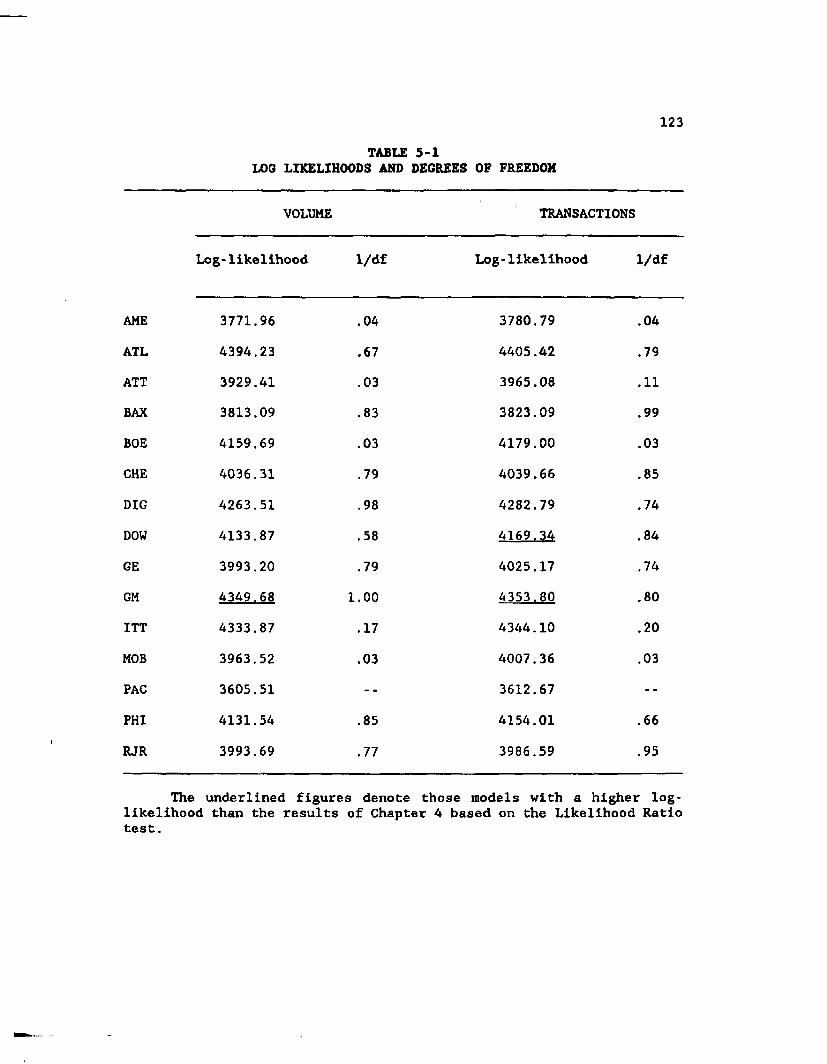
123TABLE 5-1
LOG LIKELIHOODS AND DEGREES OF FREEDOM
VOLUME TRANSACTIONS
Log-likelihood 1/df Log-likelihood 1/df
AME 3771.96 .04 3780.79 .04
ATL 4394.23 .67 4405.42 .79ATT 3929.41 .03 3965.08 . 1 1
BAX 3813.09 .83 3823.09 .99
BOE 4159.69 .03 4179.00 .03CHE 4036.31 .79 4039.66 .85
DIG 4263.51 .98 4282.79 .74DOW 4133.87 .58 4169.34 .84
GE 3993.20 .79 4025.17 .74GM 4349.68 1 . 0 0 4353.80 .80
ITT 4333.87 .17 4344.10 . 2 0
MOB 3963.52 .03 4007.36 .03
PAC 3605.51 -- 3612.67 --
PHI 4131.54 .85 4154.01 . 6 6
RJR 3993.69 .77 3986.59 .95
The underlined figures denote those models with a higher log-likelihood than the results of Chapter A based on the Likelihood Ratiotest.

124
AMEt
ATLP
ATTt
BAXp
BOEt
CHEP
DIGp
DOWp
GEp
GMP
1TTt
m o b t
PAC„
PHIp
RJRp
TABLE 5-2 ESTIMATION RESULTS - VOLUME EFFECTS
Mean equation Variance equation*1 *i Pi P* Pj P«
00 00 00
-.083 .231 .091(-6.09) (2.99) (3.97)-.016 .072 .061(-1.72) (2.06) (3.08)-.061 .033 .060(-3.17) (1.85) (5.02)-.085 .233 .151(-6.39) (3.88) (7.77)-.050 -.011 .068(-6.52) (-.39) (6.66)-.036 .015 .062(-3.26) (0.60) (6.06)-.056 .260 .067(-7.22) (12.6) (6.62)-.012 .135 ,062(-1.29) (6.01) (2.31)-.023 .196 ,067(-1.95) (6.77) (2.79)-.007 .067 .057(-1.27) (1.68) (5.65)-.026 .091 .062(-3.10) (3.61) (3.56)-.056 .060 .081(-6.23) (1.79) (6.35)-.066 .090 .080(-3.88) (1.80) (3.62)-.017 .093 .063(-1.71) (1.65) (2.92)-.023 .166 .039(-2.25) (2.65) (2.16)
0 0 0 0 0
-.208 .789(-6.65) (5.53)-.092 .039(-2.28) (0.90)-.256 .177(-8.31) (2.33)-.226 .136(-7.16) (1.37)-.270 .665(-7.17) (8.23)-.263 .326(-6.79) (2.03)-.130 .069(-6.12) (0.69)-.085 .263(-1.97) (3.29)-.190 .606(-6.31) (1.65)-.091 .056(-2.97) (1.02)-.236 .221(-7.21) (2.22)-.205 .182(-7.13) (6.78)-.567 1.56(-21.6) (3.16)-.060 .352(-1.62) (3.69)-.077 .176(-2.32) (2.67)
.000 — .179(0.02) ( 2.16)
.138 — .666(6.18) (10.62)
.019 -- .207(0.77) { 3.87)
.056 — .768(1.52) (11.56)
.151 .006(2.39) ( 0.36)
.206 — .662(3.05) ( 3.20)
.298 — .699(3.29) ( 9.26}
.229 — .222(3.98) ( 2.56)
.060 — .691(3.02) ( 2.36)
.167 — .656(2.95) ( 7.39)
.058 — .276(1.37) ( 1.66)
.076(3.28)
.060 .220 (1.66) ( 1.12).000 -- .189(0.01) ( 1.56).097 .660(2.16) ( 7.37)
0000 ooooo ooooo.368 .668 .000(3.76) (6.33) (0.00).023 .106 .000(2.06) (2.50) (0.00).017 .026 .001(1.58) (0.38) (0.62).179 .206 .000(3.08) (1.86) (0.00).052 .131 .000(3.70) (1.95) (0.00).058 .000 .000(1.75) (0.00) (0.00).000 .006 .000(0.02) (0.09) (0.00).036 .325 .000(2.01) (6.69) (0.00).001 .077 .000(0.09) (0.81) (0.00).036 .119 .000(1.88) (2.00) (0.00)
.021 .171 .000(1.79) (2.70) (0.00)
.030 .226 .002(3.18) (5.62) (0.73)
.176 .021 .000(2.70) (0.10) (0,00)
.262 .381 .000(3.02) (3.61) (0.00)
.187 .655 .000(6.26) (6.18) (0.00)The t-statistics are In parentheses.

125
AHG,
ATLp
ATTt
BAXp
BOEt
CHEp
DIGp
DOWp
GEp
GMp
ITTt
MOBt
PACh
FHIp
RJRp
TABLE 5-3ESTIMATION RESULTS - TRANSACTION EFFECTS
Mean equation Variance equation•* *1 *i *i *l 8 l 8i P4
00 00 00 OOOOO 0000 OOOOO OOOOO-.092 .169 .116 -.156 .336 .020 -- .366 .211 .003 .067(-5.69) (3.00) (5.37) (-6.69) (2.17) (0.77) ( 3.66) (6.17) (0.03) (2.03)-.023 .070 .036 -.126 .052 .065 — .719 .019 .036 .000(-2.77) (2.59) (2.97) (-3.99) (0.91) (3.28) (11.66) (2.21) (0.66) (0.00)-.060 .023 .102 -.160 .093 .017 — .367 ,086 .063 .029(-3.99) (0.56) (5.66) (-5.02) (0.56) (0.69) ( 2.25) (2.71) (0.67) (2.00)-.071 .160 .130 -.200 .665 .031 — .655 .196 .611 .000(-6.57) (3.15) (7.66) (-7.66) (1.57) (0,67) ( 2.83) (2.02) (2.56) (0.00)-.050 -.030 .069 -.261 .335 .025 .029 — .132 .121 .028(-6.56) (-.77) (6.65) (-8.36) (6.01) (0.62) ( 1.16) (5.60) (1.79) (1.20)-.036 .012 .060 -.256 .050 .163 — .568 .065 .002 .038(-3.62) (0.37) (6.66) (-7.91) (0.62) (2.63) ( 5.26) (1.76) (0.02) (1.29)-.056 .236 .069 -.11* .007 .063 — .839 .0*9 .052 .000(-7.97) (7.65) (7.21) (-6.60) (0.09) (1.97) (13.18) (3.06) (0.92) (0.00)-.013 .112 .053 -.080 .029 .165 — .619 .060 .159 .019(-1.36) (2.60) (3.77) (-2.25) (0.61) (2.66) ( 6.20) (2.12) (2.69) (1.09)-.030 .166 .069 -.166 .136 .229 — .237 .122 .256 .016(-3.26) (3.50) (6.56) (-5.19) (1.36) (3.61) ( 2.66) (2.62) (2.83) (0.83)-.010 .0*2 .058 -.086 .058 .167 — .678 .025 .032 .000(-1.36) (1.67) (5.39) (-2.52) (1.06) (3.71) ( 9.28) (1.98) (0.75) (0.00)-.025 .075 .030 -.181 .051 ,000 — .616 .063 .082 .026(-3.25) (2.25) (2.78) (-6.19) (0.81) (0.01) ( 3.12) (3.01) (1.66) (1.60)-.059 .063 .076 -.169 .316 .203 — — .308 .288 .028(-6.76) (0.63) (6.35) (-6.69) (3.50) (3.50) (6.32) (3.69) (1.25)-.072 .027 .100 -.631 .953 .1*7 .276 — - .18* .63* .000(-6.37) (0.65) (6.35) (-12.6) (2.16) (2.63) ( 1.75) (2.65) (2.27) (0.00)-.01* .107 .061 -.050 .021 .000 — .619 .221 .085 .027(-1.30) (1.31) (2.70) (-1.53) (0.39) (0.01) ( 5.10) (6.16) (1.62) (1.95)-.026 .166 .069 -.056 .086 .003 — .296 .387 .017 .053(-2.55) (2.16) (3.67) (-2.17) (0.83) (0.15) ( 2.61) (3.09) (0.19) (2.20)The t-statistics are in parentheses.

126TABLE 5-4
DISTRIBUTIONAL TESTS ON VOLUME RESIDUALS
skew kurt Sstat
X2Total
X2Tailregion
X2Midpointregion
AME -.043 0.771 0.28 160.79 2 .6 8 # 20.15
ATL - .032 2.586 0.15 281.89 3.50# 43.85
ATT -.190 0.620 5.49* 240.54 3.48# 1.18#BAX -.004 0.693 0 . 0 0 228.14 5.91# 6.48
BOE -.149 1.831 3.38 208.41 1.72# 2.79#
CHE .070 0.839 0.75 104.53 5.71# 0.65#
DIG - .018 2 . 2 0 2 0.05 43.89 2.69# 5.14#
DOW -.029 1 . 6 8 6 0.13 268.62 0.06# 22.83
GE -.290 2.275 12.74* 111.53 2.76# 17.51
GM .038 1.982 0 . 2 1 240.68 15.90 27.31
ITT - .275 1.799 11.43* 332.01 22.64 42.16
MOB -.283 2.444 1 2 .1 1 * 90.40 7.64 17.11
PAC -.262 0.067 10.42* 132.81 3.8 8 # 11.72
PHI - .359 2.922 19.49* 439.19 6.59 41.29
RJR . 1 2 2 2.161 2.25 228.43 0.62# 42.74
The x2( l ) value for the S statistic at the 0.05 significance level is 3.84. An '*' represents significance at the .05 level. A '#' indicates that the null hypothesis cannot be rejected using the goodness of fit tests.

127TABLE 5-5
DISTRIBUTIONAL TESTS ON TRANSACTION RESIDUALS
skew kurt Sstat
X2Total
X2Tailregion
X2Midpointregion
AME - . 1 0 2 0.641 1.59 104.39 0.59# 12.53
ATL .049 2.555 0.37 237.11 0 .2 0 # 33.03ATT -.097 0.247 1.44 351.17 17.34 57.36
BAX .026 0.894 0 . 1 0 485.97 8.26 3.57#BOE -.065 0.730 0.63 143.37 9.41 4.90#CHE .031 0.658 0.14 84.03 4.46# 3.45#
DIG -.049 1.799 0.37 24.59* 0.53# 10.33
DOW -.059 1.438 0.53 98.99 0.50# 5.11#GE -.063 1.005 0.60 132.13 3.22# 14.26GM -.083 1.670 1.04 175.07 7.49 42.74
ITT - .226 0.871 7.76* 439.41 32.80 31.38
HOB - . 2 1 2 1.706 6.83* 283.33 3.75# 39.99
PAC - .235 -0.017 8.35* 203.10 2 .0 1 # 8.26
PHI - .149 2.088 3.38 87.02 3.66# 24.27
RJR .044 1.759 0.29 218.88 0.06# 1.38#
The x2 (l) value for the S statistic at the 0.05 significance level is 3.84. An '*' represents significance at the .05 level. A '#' indicates that the null hypothesis cannot be rejected using the x2 goodness of fit tests.

128
TESTSTABLE 5-6
FOR NONLINEAR DEPENDENCE ON VOLUME RESIDUALS
LB(6 )r
LB(6 )r2
LB(6 )1 rl
AUTOCORRELATION FOR LAG-1 r r2 1 rf
AME 7.04 39.95* 35.69* . 0 2 0 .043 .058
ATL 7.36 7.43 11.24 .003 .057 .075
ATT 10.69 4.88 8.40 -.033 . 0 0 1 .038
BAX 10.61 6.03 5.19 - . 0 1 0 .054 .058
BOE 0.80 38.49* 34.44* - . 0 1 0 - .037 -.042
CHE 6.27 7.56 7.56 .057 -.008 -.024
DIG 19.94* 3.88 3.34 .076* .009 .018
DOW 11.15 4.31 10.16 .067 - . 0 1 1 . 0 2 1
GE 15.65* 6 6 .1 2 * 62.73* .087* .206* .174*
GM 3.99 16.43* 17.34* -.004 .066* .037
ITT 8.49 1.23 3.65 .070 .016 .030
MOB 6.15 32.75* 19.84* .033 .016 .033
PAC 6.63 24.45* 27.73* .032 .089* .079*
PHI 6.29 34.16* 41.86* -.016 .098* .1 2 0 *
RJR 4.43 7.43 12.31 .048 -.013 -.005
The critical values for the Ljung-Box, LB(6 ), statistic at the 0.10, 0.05, and 0,01 significance level are 10.64, 12.59, and 16.81 respectively. An '*' represents significance at the .05 level.
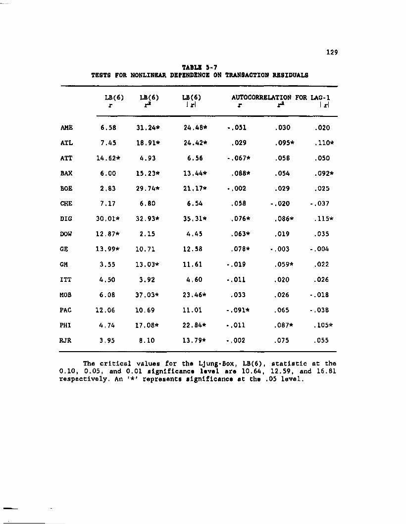
TESTS FOR NONLINEARTABLE 3-7
DEFENDENOE ON TRANSACTION RESIDUALS
129
LB(6)r
LB(6)r2
LB(6)Irl
AUTOCORRELATION FOR r r*
LAG-11 rl
AME 6.58 31.24* 24,48* -.051 .030 .020ATL 7.45 18.91* 24.42* .029 .095* .110*
ATT 14.62* 4.93 6.56 -.067* .058 .050
BAX 6.00 15.23* 13.44* .088* .054 .092*BOE 2.83 29.74* 21.17* -.002 .029 .025CHE 7.17 6.80 6.54 .058 -.020 - .037
DIG 30.01* 32.93* 35.31* .076* .086* .115*DOW 12.87* 2.15 4.45 .063* .019 .035
GE 13.99* 10.71 12.58 .078* - .003 - .004GM 3.55 13.03* 11.61 -.019 .059* .022
ITT 4.50 3.92 4.60 -.011 .020 .026
MOB 6.08 37.03* 23.46* .033 .026 -.018
FAC 12.06 10.69 11.01 -.091* .065 -.038
PHI 4.74 17.08* 22.84* -.011 .087* .105*
RJR 3.95 8.10 13.79* -.002 .075 .055
The critical values for the LJung-Box, LB(6), statistic at the 0.10, 0.05, and 0.01 significance level are 10.64, 12.59, and 16.81 respectively. An '*' represents significance at the .05 level.

CHAPTER 6VARIANCE RATIO TESTS AND ARCH EFFECTS
In a recent work, Lo and MacKinlay (1989) suggest that a variant
of the variance-ratio statistic can be used to test for the presence of
nonlinear dependence. In their paper, they specifically point out its relevance for ARCH processes. They argue that the standard variance
ratio test can be adjusted by a weighted combination of the variances of
the autocorrelations, thereby taking account of the presence of second order dependence. They conclude their work by providing a number of
simulations that favorably compare the power of this adjusted variance
ratio test to that of the Box-Pierce Q statistic and the Dickey-Fuller t tests.
In this chapter we wish to further examine the properties of this unconditional, variance-ratio statistic when the underlying return
generating process contains a specific type of second order dependence. In particular, we generate random series from a GARCH(1,1) process with
different degrees of persistence and then apply the standard and
variance, adjusted statistic to each model. In this way, we can directly
verify Lo and MacKinlay's proposition with a finite sample taken from a
population with known moments.
In the first section of this chapter, we discuss the theory behind
the standard variance ratio test and the variant developed by Lo and
MacKinlay (1989). We critique their hypothesis concerning the ability of
the adjusted test to account for ARCH type dependence. The second
section provides a description of our simulation and the Monte Carlo
130

study, along with a description of the actual return series used in the subsequent analysis. In the last section, we present our results and a discussion of their implications for our intradaily findings.
A. STATISTICAL THEORY
The concept of using the ratio of the unconditional variances from different sampling intervals to test the null hypothesis of a random
walk is not new. This time-variance relationship enjoys a long history
with particular reference to the works of Working (1949), Osborne
(1959), and the previously noted contributions of Young (1971), Schwartz
and Whitcomb (1977), and Perry (1982) [see footnote 1]. Its application to the detection of second-order dependence, in particular ARCH effects,
is the reason for the resurgence of interest in the topic.
Given a times series of log prices, liPt)t-o» sampled at some interval denoted by the unit subscript, 'i', we can express the random
walk hypothesis as xpt - iPt-i + i«t» where the !et- N(0,of). Hence the change in the series, {AjPtJJ-i, Is white noise with a variance of of (We
have referred to this series throughout this paper as rt). If we now
sample the data by using every other observation from the original
series, we obtain a series of first-differences denoted as {A2pT]?-i. In
this case, every element of (A2pt) is the sum of two adjacent elements
of (AiPt) or A2pi - AjPi + Aip2, A2p2 - Aip3 + AiP*. etc.. Diebold (1988) refers to this series as '2-aggregated' with higher order aggregates
denoted as q-aggregated for q > 2.
131

132The unconditional variances of (Ajp.), (A2p.), and (Akp.) are of,
of, and of, respectively. Under the null hypothesis of a random walk the following relationship holds:
o| - qof, q - 1,...,n/kor
2of/of - 3of/o| - ... - (n/k)of/ofA - 1.
In order to improve the power of this test, the q differences can be
based on overlapping intervals. This provides n-q+1 terms in the calculation of the aggregated series rather than only n/q terms as
defined above. We call these overlapping-interval variance ratios after
subtracting one, Mr(q), with q denoting the degree of aggregation. If the
two series forming the ratio were independent the statistics would have
central F-distributions. Since the aggregated series are not independent
of the original series, the relationship holds only at the limit and the
asymptotic distribution of (nw)Mc(q) is N(0,2[2q-1][q-l]/3q).
Diebold (1988) provides fractiles of Mr(q) for some finite sample
sizes and aggregation values. Lo and MacKinlay (1988) use unbiased
estimates of the variances in the ratio.30 They also provide a variant
30 The unbiased estimate of the unconditional variance of the first differences of the original series is:
where p is the mean of the first differences. The unbiased estimate for the aggregated series is:
(Pt-Pt-ff-w)3.

133of the statistic that purportedly adjusts for the effects of heteroskedastlcity. This variant is based on the approximation of the variance ratio statistic by a linear combination of autocorrelations. Or in notational form:
where r(.) is the autocorrelation coefficient of lag (.) and op(n"1/2)
refers to terms which are of order smaller than n'1/2 in probability.
Hence the statistic can be adjusted by the asymptotic variances of the
autocorrelations, denoted Mj). This leads to a N[0,V(q)] limiting
distribution for ME(q).31 We can then standardize the statistic to yield
Z*(q), which is equal to Mr(q)/Vtt and is distributed as N(0,1) asymptotically. Lo and MacKinlay (1989) note that the 8(j)'s are
numerically equivalent to White's (1980) heteroskedasticity-consistent covariance estimator.
where m - q(n-q+l)(1-q/n).
31 The variance V(q) is denoted by:
The 8(j) refers to the asymptotic variance of the autocorrelations of the return series and the p is the mean of same series.
Mr(q) “ 3( -x) r(l) +— r(2) + . . .+-|r(q-l)+op(n‘l/a)
where13
t £ (p.-p^-p) 2 ) 2t-i

134However, all of Che above reaulCa are baeed on Che unconditional
variances. In face the acCual simulation results reported by Lo and
MacKinlay <1989) are based on series that oontaln heterosoadaaticity but
not in the conditional variances. They point out that a
reparametrization of the variance they use would correspond to Engle's
(1982) ARCH process, but they do not explloitly examine this
possibility. In this chapter, we provide results chat do in faat account for ARCH behavior in the return series.
B. DATA AND SIMULATION DESCRIPTION
In order to carry out the Monte Carlo simulation, we create a return series, rb, with the following form:
rt - p + eb
ht - a„ + + Pihfi,
where p is the mean return and the conditional distribution of the tb Is
N(0,1). To create this series we first generate a series of normally
distributed pseudo-random variables, eb, with a zero mean and unit
variance. We then use these eb's to create a return series of the form:
- P + hi1/2ex, ra - p + h21/aea rb - p + ht1/aet,
where the starting values for h0 and eo are zero and the value of hx is equal to tc0. The remaining conditional variances are defined as:

135h2 - «„ + o^f + Pihi, h3 - a0 + «i« 2 + P2h2, •..
and so forth, where the et's equal ht1/2et. Hence, we create a return
series that Incorporates GARCH effects in the Innovations. We look at different degrees of persistence by varying the values of and px from
zero to one in the case of and from zero to nine in the case of Pi- 3 2
Note that the combination of .1 and .9 creates an I-GARCH series or a series with an infinite unconditional variance.
Because Lo and MacKinlay (1988) provide results of their test for
both an equally-weighted and value-weighted index of weekly returns, we
attempt to replicate the same series and re-evaluate their results in
the presence of GARCH. The weekly returns are calculated from the Center
for Research on Security Prices daily return file. They consist of the
Wednesday close to close price from May 2, 1974 to December 26, 1985. We
further include ten equally-weighted sized based portfolios over the
same period in the analysis. These portfolios consist of the same stocks
as the indices except they are divided into deciles based on their
capitalization value at the end of each preceding year. Hence, we have
12 returns series of 608 weeks with aggregation values, q, of 2, 4, 8 , and 16. As a final comparison, we include the estimates of the ten and
thirty minute return series for our 15 companies.
3 2 The actual Monte Carlo simulation consists of 5,000 replications for each of the values of and p^

C. SIMULATION RESULTS AND DISCUSSION136
Tables 6-1 through 6-4 provide the IX, 5%, and 10X critical values
for the 2, 4, 8 , and 16-aggregated data respectively. The first two
columns in each table give the corresponding GARCH values for and Px.
The upper portion of each table provides the critical values for the
standard variance ratio test with no adjustment for heteroskedastlclty. These ratios, after adding one, have (approximately) a central F-
distribution under the assumption that the ratio is composed of
independent variables. The lower portion contains the values for the
adjusted statistic, which have a standard normal distribution. Both
statistics are used to test the null hypothesis that the variance ratio
is equal to zero since the Mc(q) statistic has a one subtracted from it.
The first row of each table corresponds to data that is distributed N(0,1) since the GARCH parameters are set to zero in the simulation.
We first look at the results for the standard statistic for each
of the aggregation values. As the persistence in the conditional
variance is increased, the results for the standard statistic approach
zero with the right tail decreasing faster than the left. As the
aggregation value increases the values for the tails move farther from
zero indicating that the statistic is sensitive to the level of
aggregation or sample size. This is consistent with the properties of the F-distribution with different degrees of freedom.
The adjusted variance ratio statistic, in the bottom half, is
easier to interpret since it should correspond to the normal
distribution aymptotically. Hence, the critical values for the IX, 5X,

137and 10% levels should be around 2.576, 1.96, and 1.645 respectively. As can be seen from the results, the empirical distribution for our sample size Initially exhibits negative skewness in the 2 -aggregated data with
the right tail being consistently smaller than the theoretical values
and the left larger. However, this pattern is reversed in the higher
aggregations. There seems to be no general pattern in this behavior as
we vary the level of persistence using the Px parameter. Interestingly, the adjusted statistic does not seem to take account of the GARCH effects. This can be seen by the fact that the results show little
variation with or without the presence of GARCH and across any
persistence level. However, we wish to examine the behavior of this
statistic when actual data are used.
Table 6-5 provides some preliminary statistics for the ten equally
weighted portfolios and the two indices. The portfolios with the smaller size companies exhibit greater mean returns than the portfolios with the larger companies. They also have greater degrees of autocorrelation,
with the relevant coefficients moving from two to zero as we go from
portfolio one to portfolio ten. Particularly noteworthy is the presence
of second order dependence in portfolio ten and the value weighted
index, since neither exhibit first order dependence.
In table 6 -6 , we present the variance equation results of estimating a GARCH(1,1) model with a normal conditional distribution on
each of the original return series. We also provide the corresponding
variance ratio test for each aggregation level. The GARCH results
indicate a high degree of persistence with all the models exhibiting a
stationary variance process since the sum of #! and p! is less than one.

138No pattern of persistence is exhibited, although there is a gradual drop in the estimate as we move down the table. We next look at the variance ratio results.
All the ratios except two are positive, confirming the results of
the autocorrelation coefficients in table 6-5. Since a number of the return series exhibit a! estimates of around one and estimates of
about eight, we use our previous simulation results for these values to
determine the 5% significance levels. We are particularly interested in
the ratios for portfolio ten and the value-weighted index, since they
exhibit only second order dependence. We find that for the equally-
weighted index and the first nine portfolios the null hypothesis of a
random walk is rejected. This finding is expected since all these series exhibit significant autocorrelation.
However, the results for portfolio ten and the value-weighted index indicate that the ability of the adjusted variance ratio test to
detect ARCH dependence is questionable. For every aggregation level of
portfolio ten and the value-weighted index, the adjusted statistic is
unable to reject the random walk hypothesis. Yet, both series exhibit
evidence of strong GARCH effects. Thus, we must question the proposed
robustness of the test in detecting nonlinear dependence.
In the final table, table 6-7, we present the result of applying
the variance ratio tests to our intradaily data. We provide these
figures simply for comparative purposes since we do not have either the
appropriate aggregation value in our tables or the corrected ARCH
estimates. However, the results again suggest that the adjusted
statistic is not accounting for the presence of ARCH effects. Our

139reasoning Is again based on the fact that if a series exhibits only second order dependence, the variance ratio test does not seem reject
the null hypothesis. This seems to be the case for the DIG and DOU series when we compare the results of table 6-7 with those of table 3-5.
Ve note in passing that the positive lag-1 autocorrelation coefficient for RJR is dominated by a large lag- 2 negative coefficient, thereby
leading to a negative value for the variance ratio in table 6 -7 .
We conclude this chapter on a negative note. Our results indicate
that Lo and MacKinlay's proposition concerning the robustness of the adjusted variance ratio test to ARCH effects is questionable. The
failure of our Monte Carlo simulation to find any discernible difference
in the value of the test with or without GARCH effects is our first piece of contrary evidence. Our contention is confirmed when we find
that the test is unable to detect the presence of nonlinear dependence
in both the value-weighted index and the last decile equally-weighted
portfolio over the time period examined. Further support for our view is
provided by the results of the ten minute return data. Hence, we are led
to conclude that their contention is incorrect and simply adjusting the
statistic by the unconditional variances of the autocorrelation
coefficients does not improve its capacity to detect ARCH effects.

140TABLE 6-1
SIMULATION RESULTS2-AGGREGATED DATA
GARCH Standard Variance Ratio
«i PiIX level 5% level
LT RT LT RT10X level
LT RT
0 0 -0.147 0.148 -0.117 0 . 1 1 2 -0.099 0.0941 0 -0.270 0.256 -0 . 2 0 0 0.197 -0.169 0.1611 1 -0.251 0.234 -0.195 0.184 -0.166 0.1541 2 -0.248 0.242 -0.195 0.184 -0.165 0.1541 3 -0.243 0.232 -0.191 0.177 -0.162 0.1511 4 -0.238 0.224 -0.179 0.171 -0.152 0.1431 5 -0 . 2 2 2 0.217 -0.176 0.166 -0.148 0.1401 6 -0 -; 218 0.213 -0.169 0.164 -0.145 0.1371 7 -0.191 0.187 -0.154 0.152 -0.132 0.1251 8 - -ori'87 ■* Tf. 181 -0.147 0.141 -0 . 1 2 2 0.1171 9 -0.173 0.162 -0.134 0.125 -0 . 1 1 2 0.106
GARCH Adjusted Variance Ratio
“ l PiIX level 5X level
LT RT LT RT10X level
LT RT
0 0 -2.605 2.469 -2.018 1.922 -1.717 1.6220 -2.599 2.479 -2.038 1.899 -1.774 1.6081 -2.598 2.433 -2.072 1.934 -1.778 1.6382 -2.587 2.437 -2.030 1.910 -1.761 1.5793 -2.567 2.466 -2.071 1.977 -1.808 1.6334 -2.601 2.469 -2.061 1.949 -1.789 1.6225 -2.604 2.499 -2.047 1.908 -1.724 1.5806 -2.640 2.522 -2.096 1.936 -1.783 1.6317 -2.594 2.460 -2.043 1.931 -1.736 1.6288 -2.671 2.494 -1.995 1.873 -1.714 1.6079 -2.643 2.457 -2.063 1.927 -1.753 1.640

Pi
0
0
1
23456789
3H
P i
0
01
23456789
141TABLE 6-2
SIMULATION RESULTS4-AGGREGATED DATA
Standard Variance RatioIX
LTlevel
RT5X
LTlevel
RT1 0 %
LTlevel
RT
-0.246 0.271 -0.195 0 . 2 0 0 -0.167 0.168-0.332 0.387 -0.266 0.278 -0.232 0.227-0.337 0.371 -0.261 0.284 -0.223 0.231-0.336 0.385 -0.267 0.285 -0.231 0.235-0.324 0.396 -0.269 0.298 -0.228 0.237-0.317 0.392 -0.259 0.286 -0.223 0.232-0.323 0.378 -0.255 0.283 -0.223 0.226-0.320 0.388 -0.256 0.282 -0 . 2 2 0 0.228-0.301 0.350 -0.240 0.261 -0.206 0 . 2 1 2
-0.293 0.330 -0.227 0.251 -0.195 0.208-0.270 0.296 -0.213 0.219 -0.181 0.182
Adjusted Variance Ratio
IXLT
levelRT
5XLT
levelRT
10XLT
levelRT
-2.416 2.722 -1.953 2.034 -1.689 1.729-2.473 2.786 -1.944 2.028 -1.663 1.669-2.449 2.643 -1.914 2.029 -1.641 1.682-2.385 2.754 -1.890 2.035 -1.660 1.692-2.409 2.839 -1.900 2.126 -1.645 1.715-2.448 2.752 -1.932 2.068 -1.655 1.747-2.368 2.642 -1 . 8 8 6 2.009 -1.664 1.687-2.427 2.819 -1.920 2.116 -1.661 1.726-2.433 2 . 6 8 8 -1.937 2 . 0 2 0 -1.654 1.677-2.403 2.801 -1.910 2.048 -1.634 1.739-2,491 2.805 -1.951 2.070 -1 . 6 6 8 1.693
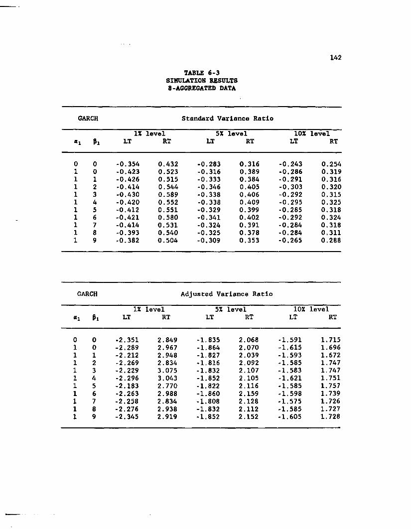
Pi
001
23456789
;h
P i
0
01
23456
789
TABLE 6-3SIMULATION RESULTS8-AGGREGATED DATA
Standard Variance RatioIX level 5X level 10X
LT RT LT RT LT
-0.354-0.423-0.426-0.414-0.430-0.420-0.412-0.421-0.414-0.393-0.382
0.4320.5230.5150.5440.5890.5520.5510.5800.5310.5400.504
-0.283-0.316-0.333-0.346-0.338-0.338-0.329-0.341-0.324-0.325-0.309
0.3160.3890.3840.4050.4060.4090.3990.4020.3910.3780.353
-0.243-0.286-0.291-0.303-0.292-0.295-0.285-0.292-0.284-0.284-0.265
Adjusted Variance Ratio
IX level 5X level 10XLT RT LT RT LT
-2.351-2.289- 2.212-2.269-2.229-2.296-2.183-2.263-2.258-2.276-2.345
2.8492.9672.9482.834 3.075 3.043 2.770 2.9882.834 2.938 2.919
-1.835-1.864-1.827-1.816-1.832-1.852-1.822-1.860-1.808-1.832-1.852
2.0682.0702.0392.0922.1072.1052.1162.1592.1282.1122.152
-1.591-1.615-1.593-1.585-1.583-1.621-1.585-1.598-1.575-1.585-1.605

Pi
0
0
1
23456789
:h
Pi
0
0
1
23456
789
TABLE 6-4SIMULATION RESULTS16-AGGREGATED DATA
Standard Variance Ratio13£ level 51 level 10X
LT RT LT RT LT
-0.499 0.628 -0.397 0.486 -0.343-0.513 0.746 -0.418 0.540 -0.374-0.543 0.778 -0.429 0.557 -0.374-0.538 0.805 -0.443 0.541 -0.382-0.531 0.817 -0.427 0.566 -0.375-0.531 0.762 -0.429 0.562 -0.380-0.532 0.774 -0.431 0.548 -0.378-0.530 0.800 -0.437 0.552 -0.388-0.528 0.763 -0.439 0.539 -0.374-0.545 0.779 -0.438 0.564 -0.376-0.521 0.739 -0.434 0.538 -0.382
Adjusted Variance Ratio
1* level 5% level 10%LT RT LT RT LT
-2.250 3.052 -1.811 2.167 -1.544-2.138 3.130 -1.793 2.219 -1.566-2.170 3.210 -1.772 2.168 -1.565-2.218 3.115 -1.796 2.196 -1.531-2.216 3.176 -1.770 2.180 -1.539-2.162 3.268 -1.768 2.247 -1.557-2.157 2.955 -1.776 2.193 -1.542-2.185 3.154 -1.792 2.225 -1.562-2.187 3.028 -1.730 2.223 -1.543-2.207 3.108 -1.753 2.247 -1.518-2.242 3.053 -1.774 2.194 -1.548

144TABLE 6-5
DESCRIPTIVE STATISTICS AMD TESTS FOR NONLINEAR DEPENDENCE ON PORTOLIOS AND INDICES
mean std dev LB(6 )r
LB(6 )
r2
LB(6 )
1 rlAUTOCORRELATION
LAG-1 LAG-2 r r
PI .00879 .0279 227.77* 49.80* 203.13* .468* .285*P2 .00616 .0253 154.26* 48.43* 115.05* .397* .229*P3 ,00552 .0242 111.08* 75.59* 102.25* .331* .190*P4 .00491 .0238 86.49* 63.11* 90.31* .304* .161*
P5 .00440 .0241 68.52* 76.66* 87.47* .280* .143*
P6 .00428 .0240 54.55* 62.23* 63.86* .248* .1 2 0 *
P7 .00403 .0227 43.97* 49,93* 61.60* .223* .109*P8 .00362 . 0 2 2 1 30.33* 43.81* 50.65* .183* .075P9 .00338 . 0 2 2 2 21.91* 56.09* 65.73* .142* .053
P10 .00261 . 0 2 2 2 7.19 57.46* 67.05* .041 .006
EW .00414 .0224 74.41* 67.73* 80.60* .281* .146*
VW .00177 .0214 5.96 67.79* 74.23* .045 . 0 1 2
The critical values for the Ljung-Box, LB(6 ), statistic at the 0.10, 0.05, and 0.01 significance level are 10.64, 12.59, and 16.81 respectively. An '*' represents significance at the .05 level. The portfolio containing the companies with the smallest capitalizaton is PI.

145TABLE 6 - 6
GARCH ESTIMATES AND VARIANCE RATIO STATISTICS OF FORTOLIOS AND INDICES
GARCH STANDARD VARIANCE RATIOVARIANCE EQUATION (ADJUSTED VARIANCE RATIO)
a o pj 2 4 8 16
PI .1470(6.04)
.5393(11.3)
.3152(6.39)
0.440(5.845)
1.082(7.413)
1.792(7.340)
2.883(5.387)
P2 .1517(5.16)
.4161(9.78)
.3608(4.92)
0.407(6.233)
0.905(7.755)
1.419(7.318)
2.197(5.043)
F3 .0476(2.56)
.1782(4.49)
.7373(1 1 .1 )
0.373(5.523)
0.800(6.917)
1.265(6.483)
1.890(4.468)
P4 .0376(2.75)
.1339(3.21)
.7944(14.7)
0.351(5.428)
0.701(6.647)
1.058(5.894)
1.629(3.830)
P5 .0498(2.32)
.1319(3.31)
.7732(1 1 .2 )
0.337(5.154)
0.684(6.123)
0.942(5.301)
1.373(3.255)
P6 .0398(2.72)
.1167(3.37)
,8071(15.7)
0.314(4.774)
0.624(5.711)
0.800(4.828)
1.059(2.755)
P7 .0441(2.29)
.1242(3.41)
.7835(12.5)
0.294(4.359)
0.595(5.209)
0.694(4.312)
0.880(2.414)
P8 .0426(2.49)
.1253(3.44)
.7825(13.0)
0.267(3.645)
0.523(4.370)
0.582(3.669)
0.777(2.093)
P9 .0149(1 .6 6 )
.0841(3.33)
.8819(23.1)
0.239(2.766)
0.482(3.361)
0.431(2.702)
0.466(1.260)
P10 .0188(1.85)
.0995(4.00)
.8588(22.5)
0.145(0.726)
0.271(1 .0 1 2 )
0.107(0.804)
0.028(-.038)
EW .0119(1.87)
.0878(3.89)
.8867(29.7)
0 . 2 2 0
(5.248)0.733(6.378)
0.917(5.709)
1.334(3.755)
VW .0158(1 .8 8 )
.1057(3.92)
.8585(23.7)
-0.050(0.963)
0.079(1.366)
0.127(1.203)
0.160(0.445)
The figures In parentheses under the GARCH estimates are the corresponding t-statistics. Those in parentheses under the variance ratios are the adjusted variance ratio statistic. The numbers refer to the appropriate aggregation value, i.e. 2 is for 2 -aggregated.

146TABLE 6-7
VARIANCE RATIO STATISTICS FOR INDIVIDUAL STOCKS
STANDARD ADJUSTEDVARIANCE VARIANCERATIO RATIO
AME -0.2348 -4.0760ATL -0.0914 -2.1315ATT -0.2515 -4.8101BAX -0.1930 -3.9956BOE -0.3655 -5.3435CHE -0.1880 -3.1815
DIG -0.0162 -0.1171DOW 0.1540 0.4197GE -0.1481 -1.0930CM -0.1656 -0.5889
ITT -0.2495 -4.1191
MOB -0.2998 -2.3603
PAC •0.6064 -9.3766
PHI -0.1623 -1.4266RJR -0.2080 -1.5101
The ratios In this table are 3-aggregated since they represent the ten and thirty minute return series.

CHAPTER 7SUMMARY AND DICUSSION OF FUTURE RESEARCH
In this dissertation, we examine (1) the time series behavior of intradaily stock prices with special emphasis on the presence of
nonlinear dependence, (2 ) the effects of aggregation in attenuating the
observed dependence in the conditional variance, (3) the role of volume
and the number of transactions as possible proxies for the rate of
information arrival to the market, and (4) the ability of the unconditional variance ratio test to detect the presence of ARCH effects.
We begin the dissertation with a discussion of the differences between the martingale model of asset prices and the random walk model.
Since the former is less restrictive is allows for certain types of dependence to exist while still maintaining those probabilistic
assumptions associated with an asset market in competitive equilibrium.
We also touch on the role that asymmetric information among market
participants plays in the realization of the actual price of each asset.
In Chapter 2, we review the literature on the distributional and
market micostructure properties of both intradaily and longer intervals.
Our discussion is generally restricted to those works that attempt to
ascertain the best model capable of accounting for the observed
empirical characteristics of the data. With Chapter 3, we begin our
actual analysis with a number of descriptive statistics, tests of
normality and white noise processes, and evidence on both the linear and nonlinear dependence found in the data.
147

148In Chapter 4, we provide the actual estimation results of applying
the generalized autoregressive condltonal heteroskedasticity model to
the the ten and thirty minute return data. Based on these results and those from Chapter 3, we posit that a mixture of distributions may In
fact describe the return generating process. The difference between this
and previous models is that such a mixture must account for the observed nonlinear dependence, as well as the distributional characteristics. Our
results suggest that the power-exponential provides a better fit to the data than either the normal or Student-t.
Chapter 5 looks at two proxies for the arrival of information to the market, volume and the number of transactions. Our intent is to
determine if the observed GARCH effects can be explained by the
information hypothesis discussed by previous authors. We find that our
sample does not exhibit any such affects and in fact application of the
proposed model raises a number of econometric problems with that
particular type of anaylsis. With Chapter 6 , we close out the result
section of the dissertation. Here we look at tfhe- robustness of the
unconditional, variance ratio test in detecting ARCH effects. We provide
evidence using both Monte Carlo simulation and actual index return data
that strongly rejects the hypothesis. 3 3
Finally, in closing, we note a number of ideas that deserve
further investigation. The first concerns the difference detected
between the beginning/end of day price process and the rest of the day.
The presence of the variance effect raises a number of interesting
3 3 We should point out that our results specifically address the null hypothesis of a random walk. If the null hypothesis is instead a martingale then Lo and MacKinlay's argument is still valid.

149questions on how the market reacts to the closing of the market. Also of interest is how aggregation of the intradaily data to daily data over a longer time span would affect the observed dependence. If daily returns,
as represented by the end of day price, are considered different from
intradaily returns then the GARCH effects may still exist at that
interval even though they do not exist in the thirty minute returns. The
second concerns the actual estimation technique we use in our analysis. Since the Student*t and power-exponential distributions are encompassed within a more general family, a natural extension is to develop the
estimation technique to accomplish this. This would allow a more direct
comparison of the two distributions based on the likelihood ratio test.
A further step would be to incorporate this extension within a mixture
of distributions framework thereby achieving a quite general
specification. Another possibility is the development of a variance ratio test that can not only account for the presence of ARCH effects
but also provide some indication of the relationship among the
conditional variances as the data are aggregated. Finally, the presence
of ARCH in return data must still be explained in terms of the way the
market prices risk. If the ARCH effects are being priced then we should
find a corresponding effect on the mean or first moment. This leads to
such models as the ARCH in mean and also to an examination of whether
the risk can be considered systematic or individual to each company. If the latter holds then traditional models such as the CAFM should still be robust to the presence of ARCH.

REFERENCESAmihud, Yakov and Haim Mendelson, Trading Mechanism and Stock Returns:
An Empirical Investigation, Journal of Finance 42 (July 1987), 533-553.
Akgiray, Vedat, Conditional Heteroscedasticity in Time Series of Stock Returns: Evidence and Forecasts, Journal of Business, 62 (January 1989), 55-80.
Akgiray, Vedat and G. Geoffrey Booth, The Stable-Law Model of Stock Returns, Journal of Business & Economic Statistics, 6 (January1988), 51-57.
Akgiray, Vedat and G. Geoffrey Booth, Compound Distribution Models of Stock Returns: An Empirical Comparison, Journal of Financial Research 10 (Fall 1987), 269-280.
Akgiray, Vedat and G. Geoffrey Booth, Stock Price Processes with Discontinuous Time Paths: An Empirical Examination, Financial Review 21 (May 1986), 163-184.
Akgiray, Vedat, G. Geoffrey Booth and Otto Loistl, German Stock Market's Resiliency to World-Wide Panics, Zeitschrift fflr Betriebswirtschaft 59 (September 1989), 968-978.
Aydogan, Kursat and G. Geoffrey Booth, Are There Long Cycles in Common Stock Returns?, Southern Economic Journal 55 (July 1988), 141-149.
Bachelier, Louis, Theorie de la Speculation, Annales de l'Ecole Normale Superiere 17 (March 1900), reprinted in The Random Character of Stock Market Prices, ed. Paul H. Cootner, Cambridge, Mass: M.I.T. Press, (1964), 17-78.
Barclay, Michael J. and Robert H. Litzenberger, Announcement Effects of New Equity Issues and the Use of Intraday Price Data, Journal of Financial Economics 21 (May 1988), 71-99.
Beja, Avraham and M. Barry Goldman, On the Dynamic Behavior of Prices in Disequilibrium, Journal of Finance 35 (May 1980), 235-248.
Berndt, E.K., B.H. Hall, R.E. Hall and J.A. Hausman, Estimation Inference in Nonlinear Structural Models, Annals of Economic and Social Measurement 3 (October 1974), 653-665.
Black, Fischer, Noise, Journal of Finance 41 (July 1986), 529-543.
Black, Fischer and Myron Scholes, The Pricing of Options and Corporate Liabilities, Journal of Political Economy 81 (May-June 1973), 637- 659.
150

151Blattberg, Robert C. and Nicholas J. Gonedes, A Comparison of the Stable
and Student Distributions as Statistical Models for Stock Prices, Journal of Business 47 (April 1974), 244-280.
Bollerslev, Tim, A Conditionally Heteroskedastic Time Series Model for Speculative Prices and Rates of Return, Review of Economics and Statistics 69 (August 1987), 542-547.
Bollerslev, Tim, Generalized Autoregressive Conditional Heteroskedasticity, Journal of Econometrics 31 (April 1986), 307 - 327.
Bookstaber, Richard M. and James B. McDonald, A General Distribution for Describing Price Returns, Journal of Business 60 (July 1987), 401- 424.
Booth, G. Geoffrey, John Hatem, Xlkka Virtanen and Paavo Yli-Olli, Stochastic Modeling of Security Returns: Evidence from theHelsinki Exchange, LSU Working Paper (April 1990).
Box, George E. P. and G. M. Jenkins, Time-Series Analysis: Forecasting and Control, San Francisco: Holden-Day, 1976.
Box, George E. P. and George C. Tiao, Bayesian Inferences in Statistical Analysis, Reading: Addison-Wesley Publishing, 1973.
Clark, Peter K. , A Subordinated Stochastic Process Model with Finite Variance for Speculative Prices, Econometrics 41 (January 1973), 135-155.
Cohen, Kalman J., Steven F. Maier, Robert A. Schwartz, and David R. Whitcomb, The Returns Generation Process, Returns Variance, and the Effect of Thinness in Securities Markets, Journal of Finance 33 (March 1978a), 149-167.
Cohen, Kalman J., Steven F. Maier, Robert A. Schwartz, and David R. Whitcomb, Limit Orders, Market Structure, and the Returns Generation Process, Journal of Finance 33 (June 1978b), 723-736.
Connolly, Robert A. , An Examination of the Robustness of the Weekend Effect, Journal of Financial and Quantitatve Analysis 24 (June 1989), 133-169.
Copeland, Thomas E., A Model of Asset Trading under the Assumption of Sequential Information Arrival, Journal of Finance 31 (September 1976), 1149-1168.
Demsetz, Harold, The Cost of Transacting, Quarterly Journal of Economics 87 (February 1968), 33-53.

152Dlebold, Francis X., Testing for Bubbles, Reflecting Barriers and Other
Anomalies, Journal of Economic Dynamics and Control 12 (March1988), 63-70.
Easley, David and Maureen O'Hara, Volume and Market Efficiency, Working Paper (November 1985).
Easley, David and Maureen O'Hara, Price, Trade Size, and Information in Securities Markets, Journal of Financial Economics 19 (September 1987), 69-90.
Engle, Robert F., Autoregressive Conditional Heteroskedasticity with Estimates of the Variance in United Kingdom Inflation, Econometrics 50 (July 1982), 987-1007.
Engle, Robert F., David F. Hendry, and Jean-Francois Richard, Exogeneity, Econometrics 51 (March 1983), 277-304.
Epps, Thomas W. , Comovements in Stock Prices in the Very Short Run,Journal of the American Statistical Association 74 (June 1979),291-298.
Epps, Thomas W., The Stochastic Dependence of Security Price Changes and Transaction Volumes in a Model with Temporally Dependent Price Changes, Journal of American Statistical Association 71 (December 1976), 830-834.
Fama, Eugene F., Mandelbrot and the Stable Paretian Hypothesis, Journal of Business 36 (October 1963), 420-429.
Fama, Eugene F. , The Behavior of Stock Market Prices, Journal of Business 38 (January 1965a), 34-105.
Fama, Eugene F. , Risk, Return, and Equilibrium in a Stable ParetianMarket, Management Science 11 (January 1965), 404-419.
Fielitz, Bruce D., Further Results on Asymmetric Stable Distributions of Stock Price Changes, Journal of Financial and Quantitative Analysis 11 (March 1976), 39-55.
Frankfurter, George M. and Christopher G. Lamoureux, The Relevance of the Distributional Form of Common Stock Returns to the Construction of Optimal Portfolios, Journal of Financial and Quantitative Analysis 22 (December 1987), 505-511.
French, Kenneth and Richard Roll, Stock Return Variances: The Arrival of Information and the Reaction of Traders, Journal of Financial Economics 17 (September 1986), 5-26.
French, Kenneth R., G. William Schwert, and Robert F. Stambaugh, Expected Stock Returns and Volatility, Journal of Financial Economics 19 (September 1987), 3-29.

153Puller, W., Introduction to Statistical Time Series, New York: John
Wiley & Sons, Inc., 1976.
Garbade, Kenneth and Zvi Lieber, On the Independence of Transactions on the New York Stock Exchange, Journal of Banking and Finance 1 (October 1977), 151-172.
Goldman, H. Barry and Avraham Beja, Market Prices vs. Equilibrium Prices: Returns' Variance, Serial Correlation, and the Role of the Specialist, Journal of Finance 34 (June 1979), 595-607.
Granger, Clive William John and Allan Paul Anderson, An Introduction to Bilinear Time Series Models, GOttingen: Vanderihoeck & Ruprecht, 1978.
Greene, Myron T. and Bruce D. Fielitz, Long Term Dependence in Common Stock Returns, Journal of Financial Economics 4 (May 1977), 339- 349.
Grossman, Sanford, Further Results on the Informational Efficiency of Competitive Stock Markets, Journal of Economic Theory 18 (June 1978), 81-101
Grossman, Sanford, On the Efficiency of Competitive Stock Markets where Trades have Diverse Information, Journal of Finance 31 (May 1976), 573-585.
Grossman, Sanford J. and Joseph E. Stiglitz, Information and Competitive Price Systems, American Economic Review 6 6 (May 1976), 246-253.
Grossman, Sanford J. and Joseph E. Stiglitz, On the Impossibility of Informationally Efficient Markets, American Economic Review 70 (June 1980), 393-408.
Haggan, V. and T. Ozaki, Modelling Nonlinear Random Vibrations using an Amplitude-dependent Autoregressive Time Series Model, Biometrika 6 8 (April 1981), 189-196.
Harris, Lawrence, A Day-End Transaction Price Anomaly, Journal of Financial and Quantitative Analysis 24 (March 1989), 29-45.
Harris, Lawrence, Transaction Data Tests of the Mixture of Distributions Hypothesis, Journal of Financial and Quantitative Analysis 22 (June 1987), 127-141.
Harris, Lawrence, A Transaction Data Study of Weekly and Intradaily Patterns in Stock Returns, Journal of Financial Economics 16 (May1986), 99-117.
Hasbrouck, Joel, Trades, Quotes, Inventories, and Information, Journal of Financial Economics 22 (December 1988), 229-252.

154Hasbrouck, Joel and Thomas S. Y. Ho, Order Arrival, Quote Behavior, and
the Return-Generating Process, Journal of Finance 42 (September1987), 1035-1048,
Heiner, Ronald A., The Origin of Predictable Behavior, American Economic Review 73 (September 1983), 560-595.
Ho, Thomas S. Y. and Hans R. Stoll, The Dynamics of Dealer Markets Under Competition, Journal of Finance 38 (September 1983), 1053-1074.
Hsieh, David A. , Testing for Nonlinear Dependence in Daily Foreign Exchange Rates, Journal of Business 62 (July 1989), 339-368.
Hsieh, David A., Modeling Heteroscedasticlty in Daily Foreign-Exchange Rates, Journal of Business & Economic Statistics 7 (July 1989), 307-317.
Karpoff, Jonathan M. , The Relation between Price Changes and Trading ' Volume: A Survey, Journal of Financial and Quantitative Analysis 22 (March 1987), 109-126.
Kendall, Sir Maurice and Alan Stuart, The Advanced Theory of Statistics (Vol 2), New York: Macmillan Publishing Co, Inc., 1977.
Keynes, John Maynard, The General Theory of Employment, Interest, and Money, New York: Harcourt Brace, 1936,
Kiefer, Nicholas M. and Mark Salmon, Testing Normality in Econometric Models, Economics Letters 11 (no.1-2 1983), 123-127.
Kon, Stanley J., Models of Stock Returns- A Comparison, Journal of Finance 39 (March 1984), 147-165.
Lamoureux, Christopher G. and Uilliam D. Lastrapes, Heteroskedasticity in Stock Return Data: Volume versus GARCH Effects, Journal of Finance 45 (March 1990), 221-229.
Leroy, Stephen F., Efficient Capital Markets and Martingales, Journal of Economic Literature 27 (December 1989), 1583-1621.
Leroy, Stephen F., Expectations Models of Asset Prices: A Survey ofTheory, Journal of Finance 37 (March 1982), 185-217.
Lintner, John, The Valuation of Risk Assets and the Selection of Risky Investments in Stock Portfolios and Capital Budgets, Review of Economics and Statistics 47 (February 1965), 13-37.
Ljung, G. M. and G. E. P. Box, On a Measure of Lack of Fit in TimeSeries Models, Biometrika 65 (August 1978), 297-303).

155Lo, Andrew W. and A. Craig MacKinlay, The Size and Power of the Variance
Ratio Test in Finite Samples, Journal of Econometrics 40 (February1989), 203-238.
Lo, Andrew W. and A. Craig MacKinlay, Stock Market Prices do not Follow Random Walks: Evidence from a Simple Specification Test, Review of Financial Studies 1 (no.l 1988), 41-66.
Mandelbrot, Benoit B., Statistical Methodology for Nonperiodic Cycles: From the Covariance to R/S Analysis, Annals of Economic and Social Measurement 1 (July 1972), 259-290.
Mandelbrot, Benoit, When Can Price be Arbitraged Efficiently? A Limit to the Validity of the Random Walk and Martingale Models, Review of Economics and Statistics 53 (August 1971), 225-236.
Mandelbrot, Benoit, The Variation of Certain Speculative Prices, Journal of Business 36 (October 1963), 394-419.
Mandelbrot, Benoit and Howard M. Taylor, On the Distribution of Stock Price Differences, Operations Research 15 (November-December 1967), 1057-1062.
Markowitz, Harry, Portfolio Selection: Efficient Diversification ofInvestments, New York: John Wiley & Sons, Inc., 1959.
McDonald, James B. and Whitney K. Newey, A Generalized Stochastic Specification in Econometric Models, Working Paper, Brigham Young University (July 1985).
McLeod, A.I. and W. K. Li, Diagnostic Checking ARMA Time Series Using Squared-Residual Autocorrelation, Journal of Time Series Analysis 4 (no.4 1983), 269-273.
Mossin, Jan, Equilibrium in a Capital Asset Market, Econometrics 34 (October 1966), 768-783.
Nelson, Daniel B., Conditional Heteroskedasticity in Asset Returns: A New Approach, Working Paper, University of Chicago (February1989).
Niederhoffer, Victor and M. F. M. Osborne, Market Making and Reversal on the Stock Exchange, Journal of the American Statistical Association 61 (December 1966), 897-916.
Oldfield, George S. Jr., Richard J. Rogalski, and Robert A. Jarrow, An Autoregressive Jump Process for Common Stock Returns, Journal of Financial Economics 5 (December 1977), 389-418.
Osborne, M. F. M., Periodic Structure in the Brownian Motion of Stock Prices, Operations Research 10 (May-June 1962), 345-379.

156Osborne, M. F. M. , Brownian Motion In the Stock Market, Operations
Research 7 (March-April 1959), 165-173.
Patell, James M. and Mark A. Wolfson, The Intraday Speed of Adjustment of Stock Prices to Earnings and Dividend Announcements, Journal of Financial Economics 13 (June 1984), 223-252.
Perry, Philip R., The Time-Variance Relationship of Security Returns: Tmplications for the Return-Generating Stochastic Process, Journal of Finance 37 (June 1982), 857-870.
Poterba, James M. and Lawrence H. Summers, Mean Reversion in Stock Prices - Evidence and Implications, Journal of Financial Economics 22 (October 1988), 27-59.
Press, S. J., A Compound Events Model for Security Prices, Journal of Business 40 (July 1967), 317-335.
Priestley, M. B, , State-Dependent Models: A General Approach to Nonlinear Time Series Analysis, Journal of Time Series Analysis 1 (1980), 47-71.
Rogalski, Richard, New Findings Regarding Day of the Week Returns over Trading and Non-Trading Periods, Journal of Finance 39 (December1984), 1603-1614.
Ross, Stephen A. , The Arbitrage Theory of Capital Asset Pricing, Journal of Economic Theory 13 (December 1976), 341-360.
Roll, Richard, A Simple Implicit Measure of the Effective Bid-Ask Spread in an Efficient Market, Journal of Finance 39 (September 1984), 1127-1139.
Samuelson, Paul A., Mathematics of Speculative Price, Society for Industrial and Applied Mathematics Review 15 (January 1973), 1-42.
Samuelson, Paul A., Proof that Properly Anticipated Prices Fluctuate Randomly, Industrial Management Review 6 (Spring 1965), 41-49.
Schwartz, Robert A. and David Whitcomb, The Time-Variance Relationship: Evidence on Autocorrelation in Common Stock Returns, Journal of Finance 32 (March 1977), 41-55.
Schwartz, Robert A. and David Whitcomb, Transaction Costs and Institutional Investor Trading Stategies, Monograph Series in Finance and Economics 2/3, New York: The Salomon Brothers Center for the Study of Financial Institutions, New York University, 1988.
Sharpe, William F., Capital Asset Prices: A Theory of Market Equilibrium under Conditions of Risk, Journal of Finance 19 (September 1964), 425-442.

157Shiller, Robert J., Do Stock Prices Move Too Much to be Justified by
Subsequent Changes in Dividends?, American Economic Review 71 (June 1981), 421-436,
Simmons, Donald M., Common-Stock Transaction Sequences and the Random- walk Model, Operations Research 19 (July-August 1971), 845-861.
Stephens, M. A. , EDF Statistics for Goodness of Fit and Some Comparisons, Journal of the American Statistical Association, 69 (September 1974), 730-737.
Stoll, Hans R., Inferring the Components of the Bid-Ask Spread: Theory and Empirical Tests, Journal of Finance 44 (March 1989), 115-134.
Tauchen, George, Discussion of 'An Investigation of Transactions Data for NYSE Stocks', Journal of Finance 40 (July 1985), 739-741.
Tobin, James, Liquidity Preference as Behavior Towards Risk, Review of Economic Studies 26 (February 1958), 6 8 -8 6 .
Veiss, Andrew A., Asymptotic Theory for ARCH Models: Estimation and Testing, Econometric Theory 2 (April 1986), 107-131.
Wood, Robert A., Thomas H. Mclnish, and J. Keith Ord, An Investigation of Transactions Data for NYSE Stocks, Journal of Finance 40 (July1985), 723-739.
Working, H., The Investigation of Economic Expectations, American Economic Review 39 (May 1949), 150-166,
Young, William E., Random Walk of Stock Market Prices: A Test of the Variance-Time Function, Econometrica 39 (September 1971), 797-812.
VITA JOHN J. HATEM
AREAS OF INTEREST Teaching
Financial Markets and Institutions
ResearchIntertemporal Asset Pricing, Trading and Price Volatility, Market Microstructure, and International Markets.
EDUCATION
Louisiana State Univ. Finance 1985-90 Ph.DYale University Molecular Biophysics
& Biochemistry 1975-80 B.S.
DISSERTATION
Topic: "The Time-Series Behavior of Intradaily Stock Prices."
An investigation of intra-day price adjustment using GARCH processes to model the observed autocorrelation and variance patterns in the return series of individual stocks.
EXPERIENCEResearch
Louisiana State University
TeachingLSU Short Courses Louisiana State University
Research Assistant 1985-90
Credit Union Finance Fall 1988 Corporate Finance 1985-90Markets and Institutions
PUBLICATIONS
"Stochastic Modeling of Security Returns: Evidence from the Helsinki Stock Exchange", with G. G. Booth, I. Virtanen, and P. Yli-Olli, European Journal of Operational Research, Forthcoming.
"A Causal Analysis of Black and Official Exchange Rates: The Turkish Case," with V. Akgiray, K. Aydogan, and G. G. Booth, Weltwlrtschaftliches Archiv, Band 125, Heft 2, 1989, 337-345.
158

159PRESENTATIONS AT PROFESSIONAL MEETINGS
"Stochastic Modeling of Security Returns: Evidence from the Helsinki Stock Exchange", (with G. G. Booth, I. Vlrtanen, and P. Yli-Olli), to be presented at 1990 SFA Meeting, Savannah.
"The Efficacy of Spread Trading Using the Gold/Silver Ratio", (with G. G. Booth and C. Mustafa), presented at 1990 SWFA Meeting, Dallas.
WORKING PAPERS
"Conditional Dependence in Precious Metal Prices", (with V. Akgiray, G. G. Booth and C. Mustafa), LSU 1990.

DOCTORAL EXAMINATION AND DISSERTATION REPORT
Candidate: John J. Hatem
Major Field: Business Administration (Finance)
Title of Dissertation: The Time-Series Behavior of Intradaily Stock Prices
Approved:
<~rldhvxessor and Chairman
Dean of the Graduate School
EXAMINING COMMITTEE.
u wc Mr/nJL
— —
Date of Examination:
June 8, 1990