The Three Epochs of Oil1

Eyal Dvir (Boston College) and Kenneth S. Rogo¤ (Harvard)

April 13, 2009

1We thank Jim Anderson, Deepa Dhume, Gita Gopinath, Lutz Kilian, BrentNeiman, and the participants of the macro seminar at BC for helpful commentson earlier versions, as well as Susanto Basu and Fabio Ghironi for helpful con-versations. An earlier version of this paper (Dvir and Rogo¤ Feb. 2008) cir-culated under the title "Oil and Global Growth." Dvir: dvire@bc.edu, Rogo¤:krogo¤@harvard.edu.

Abstract

We test for changes in price behavior in the longest crude oil price series

available (1861-2008). We �nd strong evidence for changes in persistence

and in volatility of price across three well de�ned periods. We argue that

historically, the real price of oil has tended to be highly persistent and volatile

whenever rapid industrialization in a major world economy coincided with

uncertainty regarding access to supply. We present a modi�ed commodity

storage model that fully incorporates demand, and further can accommodate

both transitory and permanent shocks. We show that the role of storage

when demand is subject to persistent growth shocks is speculative, instead

of its classic mitigating role. This result helps to account for the increased

volatility of oil price we observe in these periods.

Keywords: Oil Price, Oil Shocks, Storage, Structural Change.

JEL classi�cation: E0, Q4, L7, N5.

1 Introduction

Much has been written on the oil shocks of the 1970�s as watershed events

that have transformed the energy market; that, together with the lack of

high frequency data from earlier periods, have led to an almost complete

concentration on the post oil shock period among economists1. However,

much can be learned about oil price behavior from the less recent past. The

crude oil price time series illustrated in Figure 1 goes back to 18612; even a

cursory look reveals stark di¤erences in the behavior of the series at di¤erent

periods. First, from 1861 until about 1878, there was a period of extremely

high volatility and generally high prices. Then came a much less volatile

period, approximately between 1878-1972, in which prices were also generally

lower. Finally, from about 1972 onwards, we see a second period of high

volatility accompanied again by higher prices.

Our �rst task in this paper is to document these di¤erences and formally

test for changes in behavior. We run two such tests, for changes in persistence

and for changes in volatility. We �nd striking empirical similarities between

the periods 1861-1878 and 1972-2008, in that oil prices were both signi�cantly

more persistent and signi�cantly more volatile in these periods, both relative

to the long period that separates them, i.e. 1878-1972. We also estimate

that a further break in oil price volatility, but not in persistence, occurred

around 1934, so that the oil price in the period 1878-1934, while much less

volatile than in 1861-1878, was still signi�cantly higher than in the period

1934-19723.1Pindyck (1999) is a notable exception.2The series is taken from British Petroleum�s "Statistical Review of World Energy",

revised annually and available at www.bp.com/statisticalreview. Prices are in 2007 $USper barrel. The series is comprised of three consecutive price series: US average price in1861-1944, Arabian Light in 1945-1983, and Brent dated in 1984-2007. The 2008 datapointwas added to the BP series using oil prices from the U.S. Energy Information Agency andU.S. GDP de�ator data from the BEA.

3All of our tests reject the null of no break with a very high level of con�dence. However,the con�dence intervals around the exact break dates are large enough to suggest cautionin over emphasis on individual historical events. Our emphasis will therefore be on the

1

What can explain the concurrence of price persistence and price volatility?

We o¤er an informal, historical narrative, as well as a formal model. Our

approach in this paper is to look for a unifying framework which is �exible

enough to allow for the very di¤erent price behavior across periods that we

observe. We �nd striking historical similarities between the two end-periods

mentioned, 1861-1878 and 1972-2008, in terms of supply and demand factors

a¤ecting the market for oil. On the demand side, as we explain in greater

detail in Section 3, both periods were years of intense industrialization in

what was then becoming a major engine of the global economy: the U.S. in

1861-1878, and East Asia in 1972-2008. We see these as periods in which the

demand side was characterized by persistent growth shocks. On the supply

side, meanwhile, both periods featured uncertainty regarding the continued

access of consumer markets to oil. This was due to the monopoly of railroads

on transportation in the former period, and to the monopoly of OPEC on

easily exploitable reserves in the latter period (see Section 3 for details).

Despite the remarkable di¤erence in the scale of the oil industry between

the two periods, both monopolies had a similar e¤ect: in periods of rising

demand, they were able to restrict access to additional oil supplies, thereby

causing prices to rise.

We argue in this paper that this con�uence of supply and demand fac-

tors can explain why we observe large changes in oil price persistence over

the years: persistent growth shocks to demand, if occurring in periods in

which key players in the market had the ability to restrict access to sup-

plies, were translated to very persistent price behavior. In other words, the

monopolistic industry structure in these periods coincided with uncertainty

regarding demand trends to produce uncertainty regarding price trends. We

show in Section 3 that the change-points between periods that we identify in

our formal testing correspond to dramatic shifts in the structure of the oil

broad characteristics of the periods in question, rather than on the exact date of changefrom one period to the next.

2

industry. During periods when there were no e¤ective restrictions on access

to supplies, i.e. the industry structure was no longer monopolistic, even large

and persistent shocks did not cause more persistent price behavior. Rather,

the shocks were accommodated through a relatively quick supply response4.

Historically, this was by far the more prevalent pattern: for the most part

the history of oil has been characterized by relatively easy access to needed

oil. Consequently the market trend was quite stable from 1879 to 1971.

The historical narrative suggests reasons why certain periods would ex-

hibit substantially more oil price persistence than others, but cannot by itself

explain the observed concurrence of high persistence with high volatility. A

theoretical framework for oil should be able to accommodate both phases

of the market, and to explain both the observed persistence and volatility

behavior of oil prices. Our third contribution in this paper is to present a

model which does just that: it is an extension of the canonical commodity

storage model à la Deaton and Laroque (1992, 1996), in which we introduce

growth dynamics to their well-known framework. This results in a model that

can accommodate both I(0) and I(1) stochastic processes, so that periods of

stable and stochastic trends can both be considered. The model can explain

our main empirical �ndings: it predicts that in the presence of uncertainty

regarding the trend, rational storage behavior will act to enhance volatility.

In the standard commodity storage framework, where uncertainty is in re-

gard to deviations from trend, but the trend itself is viewed as stable, storage

acts to reduce volatility. This feature of the storage model is in itself novel,

as well as useful in terms of explaining the observed patterns in the data.

We present simulations in which this behavior can increase price volatility

following growth shocks signi�cantly.

4Examples abound: the shocks to demand imposed by the needs of the two worldwars, or by the postwar reconstruction of Europe, were large, persistent, and open-ended.However none of these major unheavals a¤ected the price of oil much. When agents triedto restrict access to supplies their e¤orts were futile, as U.S. producers learned in 1918,when the Federal government threatened to draft their workers if they did not comply(Yergin [1991], page 179).

3

The large literature on commodity price behavior falls broadly into two

major strands, depending on whether the commodity in question is perceived

to be renewable. On the one hand, models of storage have been used mostly

to study renewable commodities such as corn and wheat; see Wright (2001)

for a survey of theory and evidence5. The study of non-renewable com-

modities, a de�nition which includes oil, has followed an altogether di¤erent

path, strongly in�uenced by the seminal contribution of Hotelling (1931).

Krautkraemer (1998) surveys the theory and evidence. In the current paper

we choose storage as the more useful of the two strands. In this we are mo-

tivated primarily by the empirical evidence, which shows quite clearly that

�nite availability of oil - a separate issue from that of free access to currently

available supplies - is not of �rst order signi�cance in explaining oil price

behavior. In particular, proven world oil reserves have been increasing in

recent decades, in spite of ever increasing production6. As a result, it may

well be that technological advances in oil exploration and utilization will be

enough to satisfy demand in the foreseeable future. That is the assumption

that we make in this paper.

Our work is also related to the ongoing debate on oil and the macro-

economy (see the two recent surveys by Hamilton [2008] and Kilian [2008a]).

This literature is more interested in identifying the source of shocks to oil

prices than in specifying their type; it also deals exclusively with the post-

1973 period. We argue in this paper that a long-term view is essential to

this debate: shocks to the oil market have had remarkably di¤erent e¤ects

on the real price of oil across historical periods, not because of their origin

on the supply or the demand side, but rather because of the ability (or lack

thereof) of key players in the market to restrict access to supplies. This liter-

5A notable exception is the paper by Routledge et al. (2000), who �nd that oil pricesexhibit the strong mean reversion associated with storage models, as well as a permanentfactor. However these authors focus only on the very recent past (1992-96), and do noto¤er a theoretical justi�cation for the permanent factor.

6See BP Statistical Review (2008) for proven reserves and production data from 1980.

4

ature�s focus on recent decades can therefore be misleading: in periods when

the ability to restrict access to supplies was lacking, the oil market showed

remarkable �exibility and relative price stability, even in the face of massive

disturbances.

The paper proceeds as follows: section 2 presents our empirical �ndings

on oil price behavior over time. Section 3 puts these �ndings in the context of

the history of supply and demand for oil. Section 4 introduces the model, and

Section 5 examines the model behavior under both transitory and permanent

shocks. Section 6 concludes.

2 Behavior of the Real Oil Price: Then and

Now

Table 1 presents some simple indicators pertaining to the three periods delin-

eated in the introduction. We see that the di¤erences in mean price between

the years 1861-1877 and the years 1878-1972, at 50.9 and 17.2 respectively

(both measured in 2007 U.S. dollars), are large and statistically signi�cant

at the 1% level. Mean price between the years 1973-2008 was 44.3 (in 2007

U.S. dollars), which is signi�cantly di¤erent from the 1878-1972 mean, but at

the same time statistically indistinguishable from the 1861-1877 mean. The

same pattern holds for di¤erences in the unconditional standard deviation of

annual prices across these periods: at $25.3, the standard deviation of price

in the period 1861-1877 was signi�cantly higher than that of the period 1878-

1972 ($5.1), but statistically similar to the standard deviation of price in the

years 1973-2008 ($22.3). Examining rates of change, we see again a similar

pattern: both the mean and the unconditional standard deviation of ab-

solute price changes in the years 1861-1877 (39% and 27.5% respectively) are

signi�cantly higher than the corresponding measures in the years 1878-1972

(14.2% and 13.7% respectively), whereas the latter are signi�cantly lower

compared with the mean and standard deviation of absolute price changes

5

in the years 1973-2008 (21.5% and 22.7% respectively). Note however that

when comparing the years 1861-1877 and 1973-2008, the mean absolute price

change is signi�cantly higher in the former, while the unconditional standard

deviation of absolute price change (a common measure of volatility) is quite

similar in the two periods. In sum, Table 1 shows that there is much in com-

mon in terms of the behavior of real oil prices between the periods 1861-1877

and 1973-2008, while both periods are signi�cantly di¤erent in most respects

from the intervening period 1878-1972.

Studies of the time series properties of real oil prices have taken one of

the following approaches: ignoring these di¤erences and analyzing the series

as a whole, or else treating the series as composed of separate series "pasted

together" (in the words of Hamilton (2008)), and proceeding to analyze them

in isolation. In one important category, that of determining whether or not

oil prices exhibit a unit root, these di¤erent approaches have led to opposite

conclusions. Pindyck (1999), an example of the former approach, ignores the

aforementioned di¤erences, and judges the entire series to be mean-reverting

to a moving quadratic trend. At the opposite end, Hamilton (2008) notes the

abrupt change in the series, and proceeds to analyze the third period only

(with quarterly data). He accordingly determines that the real price of oil

follows a random walk with no drift7.

In what follows we will treat both the assumption of a pure I(0) process

and the assumption of a pure I(1) process as our null hypotheses, and test

whether the series exhibits a shift from I(0) to I(1) (or vice versa) against both

of these assumptions. In other words, instead of trying to decide whether the

series as a whole or in part exhibits a unit root, we aim to determine whether

it shows clear transitions from a stochastic trend to a deterministic one, and

vice versa. In order to do that, we employ a relatively recent test proposed

by Harvey, Leybourne, and Taylor (2006, HLT henceforth). This test is a

7Studies of higher frequency data from the 1990s (daily, weekly) do �nd a mean-reverting factor as well as a permanent factor. See for example Routledge et al. (2000),Schwartz and Smith (2000).

6

modi�ed version of a test for change in persistence proposed earlier by Kim

(2000), which itself builds on the unit root testing method of Kwiatkowski et

al. (1992). What makes the HLT test of change in persistence appealing is

that it maintains its properties of consistency and appropriate size both under

the I(0) null and under the I(1) null. This allows us to test for structural

change without taking an a-priori stand regarding the null hypothesis.

Appendix A provides an introduction to the testing method and its ra-

tionale. Table 2 presents the results of the HLT change of persistence test,

using the real oil price series. Since the test is designed to �nd a single

change-point, whereas the series exhibits two obvious break candidates, we

conducted the test separately for periods 1 and 2, and for periods 2 and

3. The exact end points shown in the table (1881 and 1965) were chosen

arbitrarily; the qualitative results are robust to small changes in these end

points8. Testing for change in persistence in the years 1861-1965, then, we

�nd very strong evidence for a signi�cant change in from a high-persistence,

local to I(1) process, to a low-persistence I(0) process, where the point of

change is estimated to be in 1877. This is shown by the very high values of

the relevant test statistics, MSR, MER, and MXR, which are all signi�cant

at the 1% level. In the period 1881-2008, we �nd strong evidence for a change

in persistence from a low-persistence I (0) process to a high-persistence, lo-

cal to I(1) process, with the point of change estimated at 1972. Again, all

three of the relevant test statistics, MS, ME, and MX, point to the same

conclusion, and all are signi�cant at the 1% level9. We use simulation re-

8As a ratio-based test, the HLT change in persistence test is designed to reject the nullif a point can be found after which the behavior of the series is statistically di¤erent thanits behavior before that point. When two such points exist, and moreover the behavior ofthe series before the �rst point is similar to behavior after the second point, this test willlose power.

9Note that for our test to reject either null, price persistence on one side of a tentativebreak should be statistically di¤erent from price persistence on the other side of the break,but need not meet any particular critical value. Because of this, Caner and Kilian�s (2001)criticism of KPSS tests, namely, that they may su¤er from size distortions and thereforeproduce spurious rejections, does not apply to our paper. Moreover, we get extremely

7

sults from Kim (2000) to calculate the 95% con�dence interval around our

change-points. As can be seen from Table 2, these are estimated somewhat

imprecisely, with con�dence intervals of 8 and 10 years for the �rst and sec-

ond change-points respectively10. However the rejection of both the null of a

pure I(0) process and the null of a pure I(1) process is quite clear, implying

that a more nuanced view of the series is in order, a view which takes into

account potential changes in persistence behavior.

Apart from the rate of persistence, another time series aspect of real oil

prices that has attracted much attention in the literature is their volatility.

As already mentioned, volatility (as measured by the standard deviation of

absolute rates of growth) was high before 1878, low from around that time

until the early 1970s, then high again until the end of our sample in 2008.

We therefore conducted a test for multiple breaks in oil price volatility, using

the methods of Bai and Perron (1998, 2003). The results are shown in Table

3, and illustrated in Figure 2. We de�ne volatility as the mean absolute

residual from a regression of oil price growth on its lagged value. The test

identi�es three potential breakpoints: 1878, 1934, and 1972. All three test

statistics against the null of no break are highly signi�cant, implying that

the series contains at least one breakpoint. However, in deciding how many

breakpoints there are, the various criteria explored by Bai and Perron do

not agree: their sequential procedure selects only one breakpoint, in 1878,

whereas the Bayesian Information Criterion selects all three11. A look at the

coe¢ cients denoting mean volatility in the di¤erent periods can explain this

discrepancy. We see that the coe¢ cients of Periods II (1879-1934) and IV

high values for our test statistics, by orders of magnitude bigger than the critical valuesgiven in the papers we rely on. Therefore the likelihood of a Caner-Kilian type spuriousrejection in our data is low.10Kim (2000) �nds in simulations that for change-points that occur at the 25th or the

75th percentile of a given series, his procedure for estimating the change-point locationhas a maximum standard deviation of 1.6893 for T=100. We accordingly use this value,scaled to our sample length, to calculate our 95% CIs.11The LWZ information criterion also chooses 1878 as the only break; however, this

criterion is known to perform badly when breaks are present (i.e. the alternative is true).

8

(1973-2008) are very similar, and both are quite di¤erent from the coe¢ cient

for Period III (1935-1972). As Bai and Perron recognize (2003, pp. 15-16),

in these cases the sequential procedure can be improved upon: the number

of breaks should be chosen according to the last signi�cant test statistic,

instead of the usual practice of choosing according to the �rst insigni�cant

test statistic. In the current case, as seen in Table 3, this improved sequential

procedure puts the number of breaks at three, similarly to the BIC. Oil price

volatility then has gone down by about half sometime in the last quarter

of the nineteenth century (with 1878 as our best estimate), then gone down

again by about two thirds around 1934. When it increased again, according

to our estimate in 1972, it regained its level of the early twentieth century,

but did not reach the heights set by oil prices before 1878. Note that 95%

con�dence intervals for the change-points are quite large; as in the change

in persistence test, our con�dence in the occurrence of breaks in the series�

behavior is far stronger than our con�dence in the exact dates of these breaks.

Nevertheless, these years will be useful as anchors in our historical narrative

in Section 3.

We can sum up our empirical �ndings as follows: real oil price from 1861-

1877 (or 1878) was highly persistent and volatile, from 1878-1934 was not

as persistent and less volatile, from 1934-1972 it was still not very persistent

and displayed even lower volatility. Finally, from 1972 on the real price of

oil returned to being highly persistent and volatile, though not as volatile as

in the pre-1878 period. Later on, in Section 4, we present a model of the

oil market that ties together these patterns of price behavior. But �rst we

need to put our model in historical context, which is the purpose of the next

section.

9

3 Industrialization andMarket Structure: Tran-

sition Points in Context

In Section 2 we identify three points of transition. In 1877-8 and again in

1972, oil price persistence and volatility both changed, while in 1934 we �nd

a change in volatility, but no change in persistence. Of these three points,

only 1934 can be linked to a major oil discovery, that of the East Texas Oil

Field a few years earlier. The other two points of transition, we will argue,

had to do with technological and geographic factors that enabled changes

in market structure. In 1878 began the construction of Tidewater, the �rst

long-distance pipeline, which eventually ended railroad monopoly over the

transportation of oil. In 1970 the East Texas Oil Field peaked, ending U.S.

control over excess exploitable reserves, and signalling the rise to prominence

of the OPEC cartel12.

These three points also show striking similarities and di¤erences from a

demand point of view as well. Of these three points, 1934 is special also in

that it occurs in the midst of a worldwide recession. Both 1877-8 and 1972

were years in which the global economy, and with it demand for oil, were

booming, driven by the large-scale industrialization of the United States and

of East Asia, respectively. Rapid industrialization is by de�nition a transi-

tional stage, and as such it features growth rates that are on the one hand

unsustainably high and on the other hand quite persistent, since the process

of industrialization often stretches over decades. In other words, periods

of rapid industrialization are characterized by persistent growth shocks to

income.

We will argue that the two observed periods in which oil prices were

12The oil industry was, of course, much bigger in the late 20th century compared to itssize a hundred years earlier; oil is also no longer used mainly for illumination as it didat �rst. It is notable however that prominent features of the industry remain relativelyunchanged: oil was internationally traded from the very beginning, demand for it beingglobal. Moreover, its e¢ ciency as a source of energy made it indispensable to consumersfrom the earliest stages, a feature of the industry that remains crucial to this day.

10

both highly persistent and highly volatile occurred because two conditions

were simultaneously met in each of these periods: access to supplies was

restricted and demand was unsustainably high. It is important to note that

U.S. industrialization was far from over when the �rst such period ended in

1878, and that post-war industrialization in East Asia was well underway by

1972, our estimate of the beginning of the second period of high persistence

and high volatility. These years were not turning points in oil demand,

rather they signi�ed major structural changes in the petroleum industry,

in which key players with the ability to restrict access to supplies either

emerged or declined in importance. When only one of the conditions was

met, as for example happened during both World Wars (when demand was

unsustainably high but supply was unrestricted), the market was signi�cantly

less persistent and less volatile. This necessary con�uence of demand and

supply factors has been relatively rare looking back all the way to 1860, but

of course has been the reality in the oil market in recent decades13.

It is worth emphasizing that we do not focus on the source of shocks

to the oil market, nor do we attempt to identify these shocks. In fact, the

model we present in Section 4 shows that growth shocks, whether to oil de-

mand or supply, can generate oil prices that are both persistent and volatile,

while AR(1) shocks, again regardless of origin, cannot. In this our paper

di¤ers from recent contributions which seek to achieve a better identi�ca-

tion of the source of shocks to oil prices in the post-1973 period (see Kilian

[2008b, 2008c]). Our main contribution is to show that to account for the

radically di¤erent behavior of oil prices across all periods, identifying the

source of shocks to the oil market may matter much less than understanding

the structure of the oil industry at the time. Studies focusing on the post-

13We stress supply restrictions rather than reserve depletion since there is no evidencethat "running out of oil" was ever a real danger. Oil security, the danger of not havingaccess to existing oil, was on the other hand very real. In this regard, "capacity constraints"must be viewed as mechanisms to restrict supply, since by their nature these constraints- derricks, strorage tanks - can be loosened in the medium run, whereas the amount ofextractable oil in any given �eld cannot be increased beyond a certain point.

11

1973 experience exclude this type of analysis by virtue of their intentionally

limited scope; empirical results pertaining to this period cannot be extended

to environments in which the oil industry�s structure is radically di¤erent.

In the �rst years of the U.S. oil industry, U.S. oil extraction was concen-

trated in a small region in northwestern Pennsylvania. Producers relied �rst

on water and horse-wagon transport to get the oil to consumers, but soon

it became clear that the only cost-e¤ective way was via rail. The railroad

companies were quick to lay down tracks to the area, so that by 1865 the

Oil Regions were well served by three di¤erent railroads. These �rms en-

joyed an oligopolistic position, as both production and re�ning were highly

competitive. That is exactly the situation that gave rise to Standard Oil:

Rockefeller envisioned a large re�ning concern that could bargain e¤ectively

with the railroads; Standard�s business advantage was well understood at the

time to consist of the special "rebates" that it was in a position to demand

from the railroads. For illustration purposes, in 1877, the year before Rock-

efeller�s succeeded in his plan, the "open fare" for rail transport of crude oil

from the Oil Regions to New York was $1.40 per barrel (Bentley [1979], page

28); this amounted to 58% of the average price of a barrel of crude oil in

that year according to our data. Williamson and Daum (1959, Chap. 17)

estimate the per barrel cost of carriage by rail at no more than $0.40 around

that time, giving us an idea of the margins involved.

In 1878 Standard Oil succeeded in acquiring not only the vast majority

of re�neries, but also all of the short-distance pipelines that connected the

oil wells to the rail tracks. This gave Standard Oil a very strong bargain-

ing position indeed, which Rockefeller proceeded to turn into large discounts

("rebates") from the railroads14. This was "the plan" all along (Yergin [1991],

Chap. 2), but it was upended quite quickly. In the same year, oil producers

who were trying to break the joint monopoly of transportation and re�ning

14Standard�s business advantage over independent re�ners as a result of its strong bar-gaining position is estimated by Bentley (1979) to have been $1.00 per barrel of re�nedoil.

12

started construction on the world�s �rst long-distance pipeline, the Tidewa-

ter. It was completed in May of 1879. In the face of this technological break-

through, Rockefeller changed his business plan and proceeded to construct

Standard�s own long-distance pipelines, choosing to destroy the railroads�

monopoly on transportation in order to strengthen Standard�s monopoly on

re�ning. This spelled the end of attempts to increase pro�tability by restrict-

ing access to oil. Having invested in his own infrastructure, and given the

very low transportation costs it a¤orded him15, Rockefeller�s strategy now

was to sell as much oil as possible: "the company needed markets to match

its huge capacity, which forced it to seek aggressively �the utmost market in

all lands,�as Rockefeller put it" (Yergin [1991], page 50). Indeed, by the early

1880�s, Standard Oil was already in bitter rivalry with exporters of Russian

oil over control of the markets in Europe and Asia.

These events occurred against a backdrop of ever rising demand, both

domestic and foreign. Oil was used for many purposes in the latter half of

the nineteenth century, of which the two most important were illumination

of homes and businesses and lubrication of machinery. The United States

was going through rapid industrialization at the time, eventually overtaking

Britain as the world�s leading center of manufacturing. During the period,

the share of world industrial output made in the U.S. rose spectacularly,

from 7.2% in 1860, to 14.7% in 1880, to 23.6% in 1900. In absolute numbers,

U.S. manufacturing production rose by a factor of three in the two decades

between 1860 and 1880, and by a factor of eight between 1860 and 190016.

U.S. population more than doubled from 1860-1900, rising from 31.8 million

to 76.4 million, while GDP per capita rose almost as fast, from $2,445 in 1860

to $4,091 in 1900 (constant 1990 dollars)17. As a result domestic consumption

15Williamson and Daum (1959, p. 458) estimate that per barrel transportation costsin Standard Oil�s own pipelines were between $0.12 - $0.20, less than half the rail cost ofcarriage.16Bairoch (1982) is the source for the U.S. absolute and relative industrial output num-

bers.17Figures for U.S. population and GDP per capita are from Maddison (2003).

13

of illuminating oil rose from 1.6 million barrels (mb) in 1873-75 to 12.7 mb

in 1899, while that of lubricating oil rose even more, from 0.2 mb in 1873-

75 to 2.4 mb in 1899 (Williamson and Daum [1959], pp. 489, 678). Even as

urban communities in the United States and Europe shifted to gas or electric

lighting, kerosene remained in high demand in other parts of the world. By

the turn of the twentieth century, there was increasing demand for gasoline,

from the burgeoning auto industry.

The transition point we identify in 1877-8 was therefore the starting point

of sweeping changes in market structure, brought about in an environment

of rapidly growing demand. Before 1878 the railroads were using their mo-

nopolistic position to limit the supply of crude to the markets in the interest

of rent extraction. After 1878 that power was slipping away from them at a

fast clip; by 1884 Rockefeller�s network of long-distance pipelines was essen-

tially complete, and the railroads were sidelined. Moreover, since Standard

Oil owned the vast majority of long-distance pipelines, and with demand

expected to continue unabated, there was no player in the market who had

both the interest and the capability of limiting supplies18. This state of a¤airs

continued until the early 1930�s (see below). With supplies limited, shocks

to demand would be fully incorporated into the price of oil. When supplies

were not limited, both demand and supply shocks would a¤ect the price.

With the trend of demand growth both before and after 1878 uncertain, we

would expect the price of oil to exhibit more persistence when demand shocks

were the main drivers, relative to when both demand and supply shocks were

driving prices.

With new �elds being discovered even as old �elds were being depleted,

supply growth was actually quite steady. The discovery of the East Texas

Oil Field changed that: from October 1930 to August 1931 oil production in

18The producers in the Oil Regions were relatively small-scale, and had repeatedly failedin their attemps to control production. There was one exception: in 1887-8, there wasa willingness to cooperate on the part of Standard Oil, and production reduction wasachieved for a short while.

14

East Texas rose from zero to over a million barrels per day (Yergin [1991],

Chap. 13). The East Texas Oil Field was by far the largest reservoir of oil

ever discovered, up to that point in time. Its discovery created an oil glut

of proportions heretofore unknown, causing a slump in price that threatened

the entire industry, and rationalizing Federal regulation. Starting in 1933,

the Roosevelt administration set quotas to the states, speci�cally designed

to curb production from East Texas. By 1937, the system had solidi�ed its

control over the non-cooperative producers: "a complete cooperation and co-

ordination... between the Federal Government and the Oil producing states

in this common e¤ort to conserve this natural resource," as the chairman

of the Texas Railroad Commission put it in a letter to Roosevelt (quoted

by Yergin [1991], pp. 258-9). The result was unprecedented control by the

U.S. government over supplies: since East Texas production was far below

its potential, and given the authority to raise and lower the quota as circum-

stances required, the U.S. government (both Federal and state, in particular

the Texas Railroad Commission) had the power to increase or decrease oil

supply almost at will. Over the decades since, while it still had that power,

the U.S. government would use it to stabilize the market on numerous occa-

sions. It increased production enormously during World War II, as well as

during supply crises involving the Middle East, in 1953 (Iran), 1956 (Suez),

and 1967 (Six-Day War). When the surge of oil was no longer needed, it had

the power to reduce production once more.

U.S. regulation thus acted as an automatic stabilizer: "setting production

to match market demand did establish a level of crude output that could be

marketed at a stable price" (Yergin [1991], page 259). This had the e¤ect of

reducing the standard deviation of supply and demand shocks, and accords

well with the observed reduction in volatility that we date to 1934, around

the time that this mechanism went into e¤ect. Quite the opposite from

the railroads�rent extraction strategy before 1878, U.S. government agencies

aimed to stabilize price by adjusting quantity as needed. The supply of oil,

15

far from limited, was in e¤ect quite �exible.

Our third transition point is 1972, where we �nd that oil price persistence

and volatility both increased. In 1970 U.S. oil production reached its peak.

In March 1971 the Texas Railroad Commission, for the �rst time since World

War II, allowed production at 100% capacity; the ability of U.S. government

agencies to increase production in times of need was gone (Yergin [1991],

pp. 567-8). Excess capacity existed now only in the Middle East, giving

the rulers of these countries the same kind of monopoly power enjoyed by

the railroads almost a century earlier: the ability to extract large rents from

consumers by limiting production19. The �rst to exercise that power was the

new ruler of Libya, Muammar al-Qadda�, who in August 1970 negotiated,

under threat of nationalization, an increase in prices and pro�ts. Other

leaders followed suit in demanding price increases, to be followed quickly by

outright nationalization of oil resources in some countries (Algeria, Libya).

In the Gulf, 1972 saw an agreement of "participation" of oil producers, i.e.

the transfer of some ownership rights of the oil resources located on their land

from the international oil companies to the governments. These developments

changed fundamentally the nature of the market: the oil producing countries

were now owners (whole or part) of their reserves, and therefore had the

direct ability to control the supply of oil to the market. In 1973, of course,

OPEC states took advantage of the October 1973 war between Israel and its

neighbors to restrict supplies dramatically.

As in the early years of the oil industry, these events were occurring

in a period of increasing demand. The demand for oil is driven, �rst and

foremost, by income. In recent decades, world GDP and global oil production

have moved in lockstep; the International Energy Agency estimates long-run

income elasticity of world oil demand at about 0.5, i.e. each percentage

point increase in world GDP is accompanied by a 0.5% increase in the global

19Smith (2008) surveys the debate on whether OPEC can be shown to have actedcollusively to withhold supplies from the market. His conclusion is that the answer is Yes.

16

demand for oil (IEA [2006,2007]). This may in fact be an underestimate:

Gately and Huntington (2002) �nd that income elasticity of oil demand in

OECD countries is 0.55, but for non-OECD countries the income elasticity

may be as high as 1. The IEA estimates that in 2001-2005, China�s higher-

than-average propensity to consume oil may have raised the global income

elasticity to 0.8 (IEA [2007]).

This time it was East Asia that was industrializing fast: �rst Japan, then

Taiwan and South Korea, and �nally China. Japan�s GDP per capita, for

example, more than tripled in two decades, rising from $3,986 in 1960 to

$13,428 in 1980. Japanese GDP by itself already equaled 37% of U.S. GDP

by 1980 (all comparisons in 1990 international dollars, Maddison [2003]).

China industrialized slightly later, but the pace of its industrialization in

the �nal decades of the twentieth century was as rapid as that of the U.S. a

century earlier, if not more: between 1980 and 2000, Chinese industrial pro-

duction rose by a factor of 9; between 1970 and 2000, it grew by a factor of

21. In relative terms, the Chinese share of world industrial output was only

0.7% 1970; it has increased to 6.3% in 200020. The IMF�s World Economic

Outlook (2008) projects that Asia�s share of global trade and manufacturing

will continue to soar in the coming decades, despite the short term disloca-

tions caused by the current �nancial crisis. Overall, the average growth rate

in Asia (excluding Japan) between 1973-2001 was 5.4%, compared with 2.1%

for Western Europe, 3.0% for the United States, and 2.7% for Japan during

the same years (Maddison [2003]). It seems clear that Asia, outside of Japan,

was still very much in the midst of an era of industrialization at the onset of

the present century, with no end in sight. This is similar to the situation of

the U.S. economy about a hundred years earlier.

We see therefore a repeat, on a much broader scale, of important features

from the market environment that prevailed before 1878: a combination of

20Statistics for China are from the World Bank�s World Development Indicators data-base.

17

supply limits and ever rising demand21. As in the earlier period, with supply

limited in this fashion, shocks to demand would be fully incorporated into

the price. Since these shocks are very persistent, in an era where the trend in

demand is uncertain, we would expect the price of oil to be more persistent,

relative to a period where these limits on supply are not binding. This

persistence in the price of oil can be reasonably expected to continue as long

as demand shocks are persistent, or until the ability of OPEC to e¤ectively

limit supplies no longer exists, either due to an independent source of oil, or

to an alternative source of energy.

4 An Extended Commodity Storage Model

Our model is an extension of the classic commodity storage framework.

Chambers and Bailey (1996) and Deaton and Laroque (1996) extend the

model to allow for autoregressive shocks. We extend it further to explicitly

incorporate demand, and to allow for growth shocks22.

4.1 Availability and Storage

Time is discrete, indexed by t. The market for oil consists of consumers,

producers, and risk neutral arbitrageurs. The latter have at their disposal a

costly storage technology which may be used to transfer any positive amount

of oil from period t� 1 to period t. Storage technology is limited by a non-negativity constraint, i.e. the amount stored at any period cannot drop below

21OECD growth was also high at various points during this time period, a fact that nodoubt has been important in the timing of the �rst and second oil shocks (see Barsky andKilian [2002, 2004]). However this fact cannot account for the very high price persistencethat we observe in this period.22Other papers which extend the storage model in various ways include among others

Alquist and Kilian (2008), Ng and Ruge-Murcia (2000), and Routlege et al. (2000). Thesepapers do not seek to explain the di¤erent behavior of oil prices across historical periodsas we do here, nor do they incorporate growth shocks explicitly into the framework.

18

zero. This implies that intertemporal arbitrage, although potentially prof-

itable, cannot always be achieved. In these cases, where the non-negativity

constraint is binding, the market is "stocked out".

De�ne oil availability, denoted At, as the amount of oil that can poten-

tially be consumed at time t. In other words, this is the amount of oil that

has already been extracted from the ground, either in period t or at some

point in the past, and has not been consumed before period t. It is given by

At = Xt�1 + Zt; (1)

where Xt�1 denotes the stock of oil transferred from period t � 1 to t, andZt denotes the amount of oil that is produced at time t. For simplicity,

we assume that no oil is lost due to storage23. Decisions concerning both

variables - how much to store, how much to produce - are assumed to have

been made before period t began. In period t agents must decide how to

divide At between current consumption Qt and future consumption, so that

demand - the sum of current consumption and the amount stored for the

future - must always equal current availability:

At = Qt +Xt: (2)

4.2 Demand for Oil

Let Yt denote a demand parameter, which can be thought of as some known

function of world GDP. Yt therefore represents the income e¤ect on the de-

mand for oil.

We can then write an inverse demand function for oil as follows:

Pt = P (Qt; Yt); (3)

23Alternatively, we could have speci�ed storage costs by a given loss percentage, as inDeaton and Laroque (1996).

19

which is decreasing in its �rst argument, and increasing in its second. This

inverse demand function constitutes a departure from the canonical model,

where demand for the commodity is a function of price only, e¤ectively as-

suming no income e¤ects. This departure is a natural one to make, however,

in the context of oil, where oil consumption and income are very highly cor-

related (see references in Section 3). Indeed, we posit an inverse demand

function in which only the ratio of consumption to income matters, so that

if both variables grow at the same rate, the price of oil will remain constant.

We assume therefore that the inverse demand function (3) is homogeneous

of degree zero:

Pt = P (Qt; Yt) = P (Qt

Yt; 1) = p(qt); (4)

where lowercase letters denote variables normalized by Yt. We think of the

normalized variables as "e¤ective" amounts, in the sense that a growing

income leads to higher energy needs, spreading any given amount of oil more

thinly. A rise in Yt would therefore, ceteris paribus, decrease the e¤ective

amount of oil available for consumption and cause a rise in current price24.

We will use a CES inverse demand function:

Pt = q� t = (at � xt)� ; (5)

where > 1 is the inverse elasticity of demand, and at, xt denote e¤ective

availability and storage in period t, respectively. It is natural to assume that

the e¤ective demand for oil is inelastic with respect to price. As equation (5)

makes clear, for a given supply of oil, price is a function of the competing

demands of current and future consumption. If the desire to consume more

in the future grows (driven by expectations of future conditions), more oil

24A disadvantage of using normalized quantities is the di¢ culty in directly calibratingthe model to actual observable quantities. This would be an important issue if we hadthe ability to perform such calibration. Unfortunately, quantity data for the oil industry -production, consumption, stocks - are not readily available for the full period (1861-2008).Our model is highly stylized as a result.

20

is stored rather than consumed today, resulting in a price rise today even

though supply has not changed.

We now turn to the speci�cation of Yt, the income e¤ect. We consider

two alternative assumptions regarding the particular stochastic process that

Yt will follow. First, we consider a simple AR(1) process, analogous to the

stochastic process that Deaton and Laroque (1996) consider for supply. In

particular, under this assumption we have

Yt+1

Y t+1

=

�Yt

Y t

��e"t+1 ; (6)

where "t+1 � N(0; �2") is an iid shock, and Y t is trend income, i.e. the level

of income that would prevail at time t in a world without income shocks.

Trend income may be constant, i.e. Y t = Y for all t, or increasing over time

at rate � > 0. The analysis of both cases will be quite similar. We think of

this case as more closely relevant to income shocks in developed economies,

where the economy exhibits business cycles around a stable trend.

Second, we will consider the case where income is subject to growth

shocks, and therefore has a stochastic trend. Speci�cally, we now assume

that

Yt+1 = e�t+1Yt; (7)

such that

�t+1 = (1� �)�+ ��t + �t+1; (8)

where � 2 (0; 1) is a persistence parameter and �t+1 � N(0; �2�) is an iid

shock. It is also possible here to express the stochastic process in terms of

the ratio between Yt and trend income Yt as in (6). Dividing both sides of

(7) by Y t+1 we get:Yt+1

Y t+1

= e�t+1��Yt

Y t

: (9)

We think of this case as more relevant to income shocks in some developing

countries, in particular quickly industrializing economies such as the U.S.

21

in the second half of the nineteenth century or China in the last decades

of the twentieth century. In these economies very high growth rates can

be extremely persistent. In principle the world price should be a¤ected by

developments in both types of economies, depending on the relative intensity

of oil use. Speci�cally, a positive income shock in an advanced economy

such as the twentieth century U.S., where the trend is stable, is expected

to disappear over time. In contrast, a positive income shock in an emerging

economy such as the late twentieth century China is perceived to have a

more lasting e¤ect, as China continues its long march towards becoming a

high income economy.

4.3 Supply of Oil

In the canonical commodity storage model, supply Zt varies according to

some stochastic process t around a predetermined mean eZt, and it is thisvariability in supply that creates an incentive for inter-temporal smoothing

by the large pool of risk neutral arbitrageurs. As the literature has long

recognized, demand and supply shocks in the canonical model are isomorphic:

one can think of a negative realization of t as representing an especially cold

winter (demand) or a breakdown in a major pipe (supply). For this reason,

since we model demand explicitly, it would be redundant to model supply

shocks separately. Our choice to model demand and not supply explicitly

has to do, of course, with the argument of Section 3.

However, supply in our model is not constant. Rather, it grows at the

trend income rate �. That is,

Zt+1 = eZY t: (10)

We include trend income Yt in equation (10) to capture the e¤ects of tech-

nological progress: next period�s supply depends on current technology. Our

assumption here is that overall technological progress, which drives global

22

GDP growth, applies to the oil extraction and exploration sectors as well.

Accordingly, while the total amount of oil existing in the earth�s crust is in-

deed �nite, technological progress is key to exploiting an increasing fraction

of it over time. Indeed, oil demand and oil production are tightly linked

in the data (IEA [2007]). Note importantly that our assumption is that oil

supply depends on the technology driving income growth, and not on income

growth itself. Therefore shocks to demand will drive a wedge between supply

and demand, causing a shift in equilibrium price. When these shocks are

lasting, as in the growth shocks case, the changes in equilibrium price will

also be lasting.

4.4 Storage of Oil

The de�ning characteristic of the canonical model is the availability of storage

technology. Private storage is essentially arbitrage: agents will buy oil and

store it if the expected future price, adjusted for �nance and storage costs,

is higher than the current price. As is common in the literature, we assume

free entry into the storage sector as well as risk neutrality, implying that the

actions of arbitrageurs will raise the current price until it is high enough to

render the strategy unpro�table in expectation. Conversely, if the expected

future price is low relative to the prevailing price, agents will reduce their

stocks, causing current price to drop. Note however that stocks cannot be

negative, limiting the e¢ cacy of inter-temporal smoothing in that case.

The amount being stored Xt and the price of oil Pt are determined to-

gether in equilibrium, given the realization of the exogenous parameter Yt.

When equilibrium at time t is fully optimal, i.e. when the storage non-

negativity constraint isn�t binding, the price of oil must obey the following

arbitrage condition:

Pt = �Et[Pt+1]� C; (11)

where � = 1= (1 + r) is the discount factor, and r > 0 is the exogenously

23

given interest rate. The parameter C > 0 denotes the per barrel cost of

storage25. Equilibrium price Pt must be such that there is no incentive to

increase or decrease Xt.

The inter-temporal price condition (11) does not hold in the case of a

stockout, i.e. the case where Xt = 0 because the storage non-negativity

constraint is binding. In this case arbitrageurs expect the future price of

oil to be su¢ ciently lower than the current price that they would sell any

amount of oil they had, except that they have nothing left to sell; every barrel

of extracted oil is being used for consumption. As a result, current price is

above its unconstrained level:

Pt > �Et[Pt+1]� C: (12)

4.5 The Rational Expectations Equilibrium

The canonical commodity storage model is a rational expectations model

with one state variable - availability of oil At - and one choice variables

- storage of oil Xt. A solution of the model - the rational expectations

equilibrium - consists of a storage rule, which speci�es the level of storage

for every possible value of the state variable. Determination of price and

consumption follows immediately from this rule26. In our extended version

of the model the rule retains its salient characteristics, well known from the

literature (see below). But in the extended version, similarly to the AR(1)

case considered by Chambers and Bailey (1996), storage is also the function

of one (or two) exogenous variables, depending on assumptions regarding the

25The cost of storing a barrel of oil have most likely decreased over time. We ignore thisfor simplicity, since accounting for a downward trend in storage cost cannot explain theobserved changes in price persistence or volatility.26Williams and Wright (1991) show that one can add an intended production rule to

the model, whereby suppliers decide one period in advance, depending on their priceexpectations, on their desired production. Our Appendix C shows how this extension canbe included in our model. However adding this second choice variable is computationallycumbersome and moreover does not add much to the insights of the model.

24

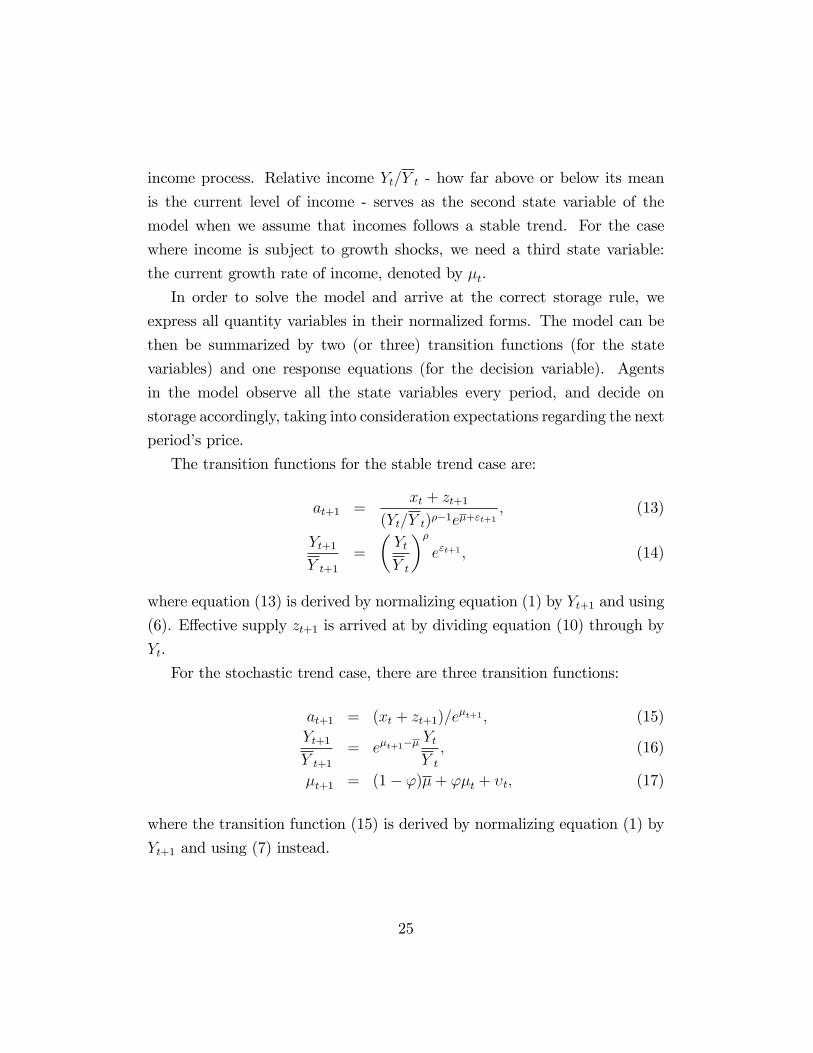
income process. Relative income Yt=Y t - how far above or below its mean

is the current level of income - serves as the second state variable of the

model when we assume that incomes follows a stable trend. For the case

where income is subject to growth shocks, we need a third state variable:

the current growth rate of income, denoted by �t.

In order to solve the model and arrive at the correct storage rule, we

express all quantity variables in their normalized forms. The model can be

then be summarized by two (or three) transition functions (for the state

variables) and one response equations (for the decision variable). Agents

in the model observe all the state variables every period, and decide on

storage accordingly, taking into consideration expectations regarding the next

period�s price.

The transition functions for the stable trend case are:

at+1 =xt + zt+1

(Yt=Y t)��1e�+"t+1; (13)

Yt+1

Y t+1

=

�Yt

Y t

��e"t+1 ; (14)

where equation (13) is derived by normalizing equation (1) by Yt+1 and using

(6). E¤ective supply zt+1 is arrived at by dividing equation (10) through by

Yt.

For the stochastic trend case, there are three transition functions:

at+1 = (xt + zt+1)=e�t+1 ; (15)

Yt+1

Y t+1

= e�t+1��Yt

Y t

; (16)

�t+1 = (1� ')�+ '�t + �t; (17)

where the transition function (15) is derived by normalizing equation (1) by

Yt+1 and using (7) instead.

25

The response equation for both cases is:

(at � xt)� = �Et[Pt+1]� C: (18)

Note importantly that equation (18), which determines optimal storage,

holds only when the state variables are such that the optimal storage is

non-negative. If the state variables dictate negative storage, this response

condition breaks down and we have simply Pt = a� t .

The existence and uniqueness (under certain general conditions) of the

rational expectations equilibrium, as well as its important properties, have

been proven in the literature. In particular, Chambers and Bailey (1996)

prove these properties for the case of auto-correlated supply shocks. How-

ever, commodity storage models generally cannot be solved analytically even

in their most simple form, due to the non-negativity constraint. We there-

fore follow the literature since Gustafson�s (1958) original contribution and

proceed to solve the model numerically. This can be done using a variety of

methods27. For computational reasons, we choose to use the spline colloca-

tion method (see Judd [1998], Miranda and Fackler [2002] for a discussion),

details of which are given in Appendix B.

The storage rules in our extended model are identical in form to the

ones that result from the canonical model. The di¤erence is that in the

extended model these rules hold for the normalized variables instead of the

original quantities. In other words, e¤ective storage has a relationship with

e¤ective availability in the extended model, under both sets of assumptions

regarding demand, that is qualitatively similar to the relationship between

actual storage and actual availability in the canonical model.

Figure 3 exhibits the optimal storage rule as well as the corresponding

equilibrium price, both as functions of e¤ective oil availability at (on the

27Williams and Wright (1991), Chap. 3, survey the numeric methods applied to com-modity storage models in the literature.

26

horizontal axis), with the other state variable(s) held constant28. The �gure

is qualitatively similar regardless of our assumption on income�s stochastic

process.

Figure 3 Here.

In the �gure, points on the curves that correspond to a particular level of

e¤ective availability represent the rational expectations equilibrium - e¤ective

storage and the resulting equilibrium price - that would prevail if e¤ective oil

availability were indeed at that level. As illustrated in the �gure, e¤ective

storage is zero when the e¤ective amount of oil available is low, then after a

kink at a it rises monotonically29. The marginal propensity to store is always

less than one; that is because a rise in storage must lower the expected future

price, as it raises future availability of oil. The kink in the storage rule occurs

when an additional barrel of stored oil will generate an expected pro�t of zero:

a� = �E[z� ]� C; (19)

where z, recall, is normalized production (which is a function of current and

trend income; see below).

Importantly, the kink at a is also seen in the equilibrium price function

p: when oil is relatively abundant, i.e. a > a, the price function is more

elastic. That is because once storage kicks in, a rise in oil availability causes

a less than proportionate rise in the amount available for consumption, since

28Certain assumptions need to be made regarding the model�s parameters in order tosolve the model numerically. Demand elasticity �1= is set at -0.2. The cost of storage Cis 0.02 per barrel. The discount factor � is set at 0.97. E¤ective supply capacity eZ is setat 1.3. The trend income growth rate � is set at 0.02, while the persistence parameter �is set at 0.5. Lastly, the income shock�s standard deviation � is set at 0.01.29See Deaton and Laroque (1992), Theorem 1. When availability is relatively low (oil is

temporarily scarce), agents will sell o¤ all existing inventories of oil while the equilibriumprice is high, expecting it to fall in the following period. Storage will be therefore zero,and indeed would have been negative had it been possible - agents would want to hold ashort position.

27

there is now competing demand from arbitrageurs who are keen to increase

their stocks. As a result, equilibrium price is less sensitive to changes in

availability when storage is positive relative to a stockout situation where

this competing demand is non-existent.

As shown by Chambers and Bailey (1996), the rational expectations equi-

librium is generally dependent not only on current availability, but also on

the current shock. Figure 4 therefore examines how the storage rule and

the equilibrium price change with current income, given by Yt=Y t, when in-

come is subject to shocks around a deterministic trend. This exercise is

very similar to Chambers and Bailey, with similar results: since shocks ex-

hibit positive auto-correlation, a higher than average income today leads to

a higher expected future income, implying that at any level of e¤ective avail-

ability, arbitrageurs will raise the optimal amount of storage in expectation

of higher prices next period. This, in turn, leads to a higher equilibrium price

today wherever storage is positive.

Figure 4 Here

When income is subject to growth shocks the model behaves in a very

similar way: when current income is high relative to its trend, or when the

current growth rate is relatively high, we would see the storage rule shifting

up and to the left, with the equilibrium price rising accordingly. Intuitively,

the logic is straightforward: when income is subject to growth shocks rather

than autocorrelated level shocks, it is still the case that a current income

that is high relative to trend predicts relatively high income in the future.

Therefore the storage rule and the equilibrium price should respond in a

similar way. When the current growth rate is relatively high, this implies a

higher-than-average growth rate in the future, given our assumption of au-

tocorrelation in growth rate, transition equation 17. That again leads agents

to expect higher income in the future, which works in the same direction. We

see then that the introduction of growth shocks does not change the char-

28

acteristics of equilibrium in the model. It will, however, change its dynamic

behavior, an issue to which we turn next.

5 Dynamic Behavior of Storage and Price in

the Extended Model

We can now examine the dynamic behavior of the model following shocks to

the income process. We �rst examine the dynamic behavior of our extended

model under the assumption that shocks to income are AR(1), and show

that our extended model behaves very similarly to the model analyzed and

estimated by Deaton and Laroque (1996). In particular, storage in these

conditions serves its classic purpose, to mitigate shocks: arbitrageurs transfer

stocks from times of plenty to times of want. Therefore storage cannot explain

price volatility. We then proceed to show that the model�s dynamic behavior

is quite di¤erent when we assume that demand is subject to growth shocks.

Storage will act to magnify shocks in the model, thereby increasing price

volatility30.

5.1 AR(1) Shocks to Income

Consider �rst a positive and persistent shock to income, when the stochastic

process is AR(1). The shock�s e¤ects on e¤ective availability, equilibrium

price, e¤ective production, and e¤ective storage are depicted in Figure 5.

The �gure exhibits the results of the following simulation: we let the system

run for 30 periods, where each period a new value of "t is drawn from the

appropriate distribution. We perform 100,000 repetitions of this simulation,

30Kilian (2008c) argues that oil price movements that cannot be explained by either sup-ply or industrial demand shocks should be thought of as shocks to precautionary demand.The endogenous storage response in our model is also separate from the direct e¤ects ofthe shock, however it responds to the expected mean price, rather than to its expectedvolatility as is the case with precautionary demand.

29

with the �gure showing mean values for each period. This produces the

baseline case. We then repeat this exercise with one change, namely that in

period 2 there occurs a three standard deviation positive shock to "t. The

mean results of 100,000 repetitions of this simulation are shown in dashed

lines.

The shock to income results in e¤ective availability dropping sharply,

leading therefore to an immediate rise in current equilibrium price, as a

�xed amount of oil must satisfy a larger thirst for it. These twin e¤ects on

e¤ective availability and price subside gradually over time, as the income

shock dissipates, and the system returns to its steady state. Oil production

is inelastic in our model, implying that e¤ective oil supply will drop with the

shock, only to recover slowly as the shock dissipates31.

The shock�s e¤ects on storage are more complex. Arbitrageurs are caught

between two contradictory forces following this type of shock: on the one

hand, the rise in current prices and drop in current e¤ective availability

dictate a drop in optimal e¤ective storage according to the storage rule (see

Figure 3). On the other hand, due to the shock�s persistence future income

is also expected to be higher than average, implying higher expected future

prices and therefore an increased incentive to store at any level of e¤ective

availability (see Figure 4). However, the former e¤ect must dominate the

latter in the case of an AR(1) income process, as future income is expected

to be less than current income, implying that future e¤ective availability is

expected to be higher than its current value, and accordingly that the future

price is expected to be lower than its current, post-shock level. As a result,

the e¤ect of a positive shock to income would be to reduce storage until the

system reverts back to its steady state.

31If production were elastic, as in Williams and Wright (1991), producers would respondto these developments by increasing their planned production in expectation of higherprices. As seen in the analytically solvable no-storage case (see Appendix), the elasticityof planned production with respect to current income is less than one, due to the positiveslope of producers�marginal cost curve. E¤ective production would respond therefore ina qualitatively similar way if production were not perfectly inelastic.

30

Figure 5 Here.

We see in the system�s response to a temporary and persistent demand

shock the underlying reason for the disappointment expressed by Deaton

and Laroque (1996) regarding the storage model�s inability to account for

the auto-correlation seen in commodity prices. When shocks are transitory,

i.e. when the system is stationary, storage acts as a countervailing force: in

Figure 5, when the equilibrium price is above its steady state level, storage

is smaller than its own steady state level, in a partial compensation for the

shock. This in itself does contribute to a higher equilibrium price in the

next period, as observed in the data. However, persistence of the shock only

serves to reduce the magnitude of this response, since the connection between

current and future conditions formed by the shock�s persistence substitutes in

part for the inter-temporal connection that is due to arbitrage. Therefore an

AR(1) shock does not deliver the added persistence that Deaton and Laroque

(1996) are looking for.

5.2 Growth Shocks to Income

Our extended model allows us, as we have seen, to incorporate growth shocks

into the storage framework. In this case, storage does not act as a counter-

vailing force anymore; indeed, immediately following the shock storage tends

to magnify the shock�s e¤ect on equilibrium price. Figure 6 demonstrates

the e¤ects of a positive and persistent shock to income growth, in this case a

three standard deviation positive shock to �t. As in the AR(1) case, a positive

demand shock lowers e¤ective availability and raises the equilibrium price.

However, in this case the shock brings about a transition to a new steady

state in which e¤ective availability is expected to be at a lower level perma-

nently, accompanied by a permanently higher price level, and a permanently

lower e¤ective production level. Importantly, due to positive auto-correlation

in the stochastic process, this transition is spread over several periods. This

31

provides a role for storage. As in the AR(1) case, arbitrageurs are subject to

contradictory forces: the current rise in price induces a corresponding drop

in storage, while the prospect of higher prices in the future induces a storage

increase. However, the crucial di¤erence between the two cases is that here,

due to the shock�s persistence, equilibrium price in the future is expected to

increase relative to the current, post-shock price. As a result, in the sto-

chastic trend case the storage-increasing e¤ect of future prices is stronger

than the storage-decreasing e¤ect of the current price. Storage in the tran-

sition period is therefore higher in expectation relative to the expected path

it would follow had the shock not occurred. In the stochastic trend case, the

shock�s persistence magni�es the storage response instead of diluting it as in

the stable trend case32. Note that if growth shocks were iid, there would be

almost no storage response: the price determined by the current period shock

would be expected to persist in the future, so there would be no incentive to

change the amount of optimal storage chosen before agents gained knowledge

of the shock.

Figure 6 Here.

It is revealing to compare our simulated response to the case where stor-

age is not allowed. This is done in Figure 7, where the post-shock expected

paths of the endogenous variables are compared with the paths these vari-

ables would take if storage were not possible. Due to the shock to income

growth, storage spikes sharply upwards, leading to a slightly higher equilib-

rium price relative to the no-storage case. E¤ective availability in the periods

of transition to the new steady state is high relative to the no-storage case,

since storage remains positive throughout the transition (in expectation of

higher prices in the future). Therefore we see a slower expected convergence

to steady state price relative to the no-storage case.32The same logic applies to the opposite case, where income growth su¤ers a negative

shock, but with a caveat. Storage response, in this case a decrease, is stronger the morepersistent the growth shock. However, since storage cannot be non-negative, this e¤ect isbounded in the negative growth shock case.

32

Figure 7 Here.

We see then that in the presence of growth shocks, a rise in current price

may be associated with an increase in optimal storage, rather than a decrease

as would always be the case in the canonical model. Storage in this case does

not "lean against the wind", as is its customary role; it actually magni�es

the shock somewhat, by increasing demand exactly when it is already high,

in preparation for even higher demand in the future. This behavior could

act to increase price volatility above and beyond what it would otherwise

be without storage. In fact , when we simulate the model with and without

storage, we �nd that price volatility following a growth shock is indeed higher

when storage is present. Figure 8 shows the results of these simulations. As

before, we let the model run for 30 periods, simulating the evolution of prices

and quantities after a positive growth shock to income. We then repeat the

process 100,000 times. Each time the model is run, we regress the growth rate

of price on its lag, and use the absolute value of the residuals as our measure

of volatility (the same measure that we used in testing for di¤erences in

volatility of real oil price data in Section 2). Figure 8 presents the mean

value of this measure, per period, for the case where storage is allowed, and

for the case where it is constrained at zero. We see that the initial positive

growth shock results in much higher price volatility - roughly double with

the parameters assumed here - when storage is allowed, and that the e¤ect

lasts for several periods until price volatility converges back to its long run

mean33.

Figure 8 Here.

In our extended commodity storage model with growth shocks, we have

arrived at a result that accords well with our empirical �ndings: periods

33Recall that our persistence parameter here is set at � = 0:5. Our qualitative resultsstand with higher or lower persistence.

33

in which persistent growth shocks are dominant should be periods in which

price exhibits extra volatility, relative to periods in which AR(1) shocks are

more prevalent. In quantitative terms, our simulations show that storage

alone can double, on average, the volatility of prices immediately after a

positive growth shock. This di¤erence is of a similar order of magnitude to

the di¤erences in price volatility that we observe in the data. This tells us

that the mechanism which we emphasize in this paper can go a long way

towards accounting for the di¤erences across periods in the complete time

series of real oil price.

6 Conclusion

We argue in this paper that a long-term view is essential to understanding

the dynamic behavior of oil prices. We show that shocks to the oil market

have had remarkably di¤erent e¤ects on the real price of oil across historical

periods, but not because of their origin on the supply or the demand side,

rather because of the ability (or lack thereof) of key players in the market to

restrict access to supplies. In other words, it is the con�uence of demand and

supply factors that determines the e¤ects of shocks to the oil market. With

e¤ective restrictions on access to excess supplies, growth shocks can generate

oil prices that are both highly persistent and, through an endogenous storage

response, highly volatile. On the other hand, without these restrictions, the

same growth shocks will be quickly accommodated, and will not lead to

increased persistence or volatility. In this regard, it is immaterial whether

the growth shocks originate on the demand or the supply side.

The literature�s focus on the extremely persistent and volatile post-1973

period can therefore be misleading: throughout most of the history of oil, the

ability to restrict access to supplies was actually sorely lacking, with the oil

market showing remarkable �exibility and relative price stability as a result.

This held true even in years when oil supply or demand were experiencing

34

great upheavals, such as during World War II and the postwar re-building of

Europe. The history of the oil industry shows that shifts in industry structure

can occur quite quickly; the structural breaks in price behavior associated

with these shifts are testimony to their importance.

A Testing for Change in Persistence

What follows is a brief introduction to the method of testing for change in

persistence we apply in the paper, and to the test statistics constructed when

using it. Consider a time series yt, where t = 1; :::; T . Assume the series can

be decomposed into the sum of a deterministic trend, a random walk, and a

stationary error:

yt = �t+ rt + "t; (20)

where rt is the random walk component:

rt = rt�1 + ut: (21)

Let the errors ut be iid with mean zero and variance �2u. Then one can test

the null hypothesis of I(0) by positing H0 : �2u = 0 against the alternative

H1 : �2u > 0. The test is constructed as follows: let et denote the residuals

from a regression of yt on an intercept and a trend. Then consider the

following test statistic:

K =1b�2"

TXt=1

S2t ; (22)

where b�2" is the estimated error variance, and St denotes the partial sum

process:

St =

tXi=1

ei; t = 1; :::; T: (23)

A value of this test statistic that is higher than an appropriate critical value

would imply a rejection of the I(0) null. Kim (2000), later modi�ed and

35

corrected by Kim et al. (2002) and Busetti and Taylor (2004), apply this

method to the question of change in the rate of persistence of a series. With

the same null hypothesis, consider the following two alternative hypotheses:

H01 :

(�2u = 0; t = 1; :::; �T

�2u > 0; t = �T + 1; :::; T; (24)

H10 :

(�2u > 0; t = 1; :::; �T

�2u = 0; t = �T + 1; :::; T: (25)

The point �T at which the change from I(0) to I(1) (under H01) or vice

versa (under H10) is assumed unknown, and is estimated during the testing

procedure. The test is carried out as follows. At each possible change-point

(say, at all points in the range [� lT; �uT ]), compute two sets of residuals: let

et denote the residuals from a regression of yt , t = 1; :::; �T on an intercept

and a trend, and let eet denote the residuals from a similar regression for the

observations t = �T + 1; :::; T . We can then de�ne the partial sum processes

accordingly:

eSt =tX

i=�T+1

eei; (26)

St =tXi=1

ei: (27)

Note that by construction the test allows for the possibility of a break in

both intercept and trend at the possible change-point. For all � 2 [� l; �u]de�ne the following statistic:

K[�T ] =[T (1� �)]�2

PTt=�T+1

eS2t[�T ]�2

P�Tt=1 S

2

t

: (28)

Had � been known with certainty, this statistic (evaluated at �) could be

36

used to test the null of a pure I(0) process against the alternative H01. A

high value of the statistic would imply a rejection of the I(0) null. Since in

general the true � is not known, Kim(2000) suggests using three functions

of the sequence of K[�T ] over the range � 2 [� l; �u]. The limits � l; �u arearbitrarily chosen, commonly 0:2 and 0:8, respectively. The three functions

are given by:

MS =1

�u � � l + 1

�uTXt=� lT

Kt;

ME = log

"1

�u � � l + 1

�uTXt=� lT

exp (Kt)0:5

#;

MX = maxt=� lT;:::;�uT

Kt:

Busetti and Taylor (2004) show that it is possible to use the reciprocal

of Kt to test the I(0) null against H10. We can de�ne the functions MSR;

MER, MXR in a similar manner, substituting K�1t for Kt everywhere. A

third set of test statistics can be used to test the null against any change in

persistence, whether from I(0) to I(1) or vice versa. These are de�ned as

follows:

MSM = maxfMS;MSRgMEM = maxfME;MERgMXM = maxfMX;MXRg

Further, HLT show that all nine statistics, in a modi�ed form, can also

be used to test an I(1) null against H01, H10, or both. The modi�cation they

propose is meant to counter spurious rejections of the null which may occur

if we ignore the possibility that the true model is indeed I(1), i.e. make sure

that the test statistics have the correct size under both I(0) and I(1). HLT

show that this can be achieved by multiplying the relevant test statistic by

37

exp(�bJ), where b is a constant, and J denotes the Wald statistic for testingthe joint hypothesis that in the following regression:

yt = 0 + 1t+ 2t2 + :::+ 9t

9;

the coe¢ cients of all higher order trends (i.e. 2; :::; 9, quadratic trend and

above, in the standard case) are zero. HLT also allow for the test to include

local to unit root behavior as well as true unit root behavior, so that H01can

be thought of as a signi�cant change in persistence from I(0) to a rate of

persistence that is very close to 1, but not necessarily exactly 1. The same

holds for H10.

A �nal step in the testing procedure, taken only if the tests indicate that a

change in persistence has indeed taken place, is to estimate the change-point

�T . Kim (2000) suggests the formula:

�(�) =[T (1� �)]�2

PTt=�T+1 ee2t

[�T ]�2P�T

t=1 e2t

;

where, in the case of rejecting the null in favor of H01, the estimated change-

point is:

� 01 = arg maxt=� l;:::;�u

�(�);

and in the case of rejecting the null in favor of H10, the estimated change-

point is:

� 10 = arg mint=� l;:::;�u

�(�):

B Production when Storage is Impossible

When inter-temporal storage is ruled out by assumption, we can analytically

express intended production as a function of current variables and the para-

meters of the model. This is no longer possible when storage is introduced.

This appendix shows the basis for intuitions given in the main paper.

38

The expected future price Et[Pt+1] under this assumption is given by

Et[Pt+1] = Et[at+1� ] = Et

"�Zt+1Yt+1

�� #: (29)

Given our assumptions regarding functional form, this can be written either

as

Et[Pt+1] =

eZt+1Yt

!� �Yt

Y t

� (��1)e �Et[e

("t+1� t+1)]; (30)

in the case of income following an AR(1) stationary process, or as

Et[Pt+1] =

eZt+1Yt

!� Et[e

(�t+1� t+1)] (31)

in the case of income exhibiting a stochastic trend. From the supply rela-

tionship (10), we have that optimal intended e¤ective production is

eZt+1Yt

=

�Yt

Y t

��1(Et[Pt+1])

�: (32)

Plugging this into the expected price expression for the stationary income

case (30) we get

eZt+1Yt

=

"�Yt

Y t

� �(��1)�1e �[��' t+ (�

2"+�

2!)=2]

#1=(1+ �); (33)

and using instead the expected price expression for the case where income is

subject to growth shocks, we get

eZt+1Yt

=

"�Yt

Y t

��1e �[(1��)�+��t�' t+ (�

2�+�

2!)=2]

#1=(1+ �): (34)

Note that the elasticity of optimal intended production with respect to

39

current income (equal to � �=(1+ �) in the stable trend case, or �=(1+ �)

in the stochastic trend case) is always less than one. This is the standard

result of general supply and demand analysis, due to our assumption that

marginal cost has a positive slope: producers optimize by increasing produc-

tion in the face of increased demand, but increase it at a lower rate. In other

words, e¤ective intended production eZt+1=Yt is always a decreasing functionof current relative income, the ratio of actual income to trend Yt=Y t. The full

numerical solution of the model, with storage allowed, this intuition applies

as well.

It is also worth noting how e¤ective intended production responds to

current shocks in the no-storage case. A positive shock to the supply level -

a high value of t - will lower e¤ective intended production. This is due to

positive auto-correlation, as a higher supply today raises expectations for a

higher supply, and lower prices, tomorrow. This naturally leads to a producer

response of decreasing intended production. The opposite occurs following

a positive shock to demand growth - a high value of �t - which will increase

e¤ective intended production. This is also due to positive auto-correlation,

here in growth rates: higher income growth today leads to expectations of

higher than average income growth in the future, implying higher prices in

the future and therefore an increased incentive to produce.

C Solving the Model

We solve the model numerically using spline collocation. The following sum-

marizes the logic of this method, using as an example the simplest case of

one state variable and one choice variable. More complicated versions of

the model are solved in exactly the same way, adding more conditions as

appropriate.

The collocation method approximates an unknown function (in this case,

the equilibrium price function) by a linear combination of known functions

40

of the state variable:

f(A) = P (A�X(A)) �NXn=1

bn�n(A): (35)

Approximating the price function leads to better results compared with ap-

proximating the storage rule directly, since the former function is relatively

smoother. It is always possible to express the equilibrium price function in

terms of the storage rule and vice versa, as shown above.

The collocation method chooses N points in the state variable�s support,

the collocation nodes, and stipulates that the equilibrium condition (11) must

hold exactly at these nodes. This reduces the problem�s dimensionality from

in�nity to N ; there are N nonlinear equations, one for each collocation node,

and correspondingly N coe¢ cients bn to be determined. We choose cubic

splines as the known basis functions �n(A).

The expectation operator is dealt with by a discretization of the known

distribution of the shock, i.e. by assigning probabilities wk to particular

points on the distribution�s support "k, where k = 1; :::; K, such that the

continuous density is approximated by the two vectors ("k; wk). The method

then proceeds to �nd the coe¢ cients of the linear approximation by using a

double iteration. First, given an initial guess for the coe¢ cients bn, it �nds

the values of the choice variable for which the equilibrium condition holds at

the collocation nodes. The equilibrium condition at node i must then hold

exactly, allowing us to solve for Xi:

P (Ai �Xi) = �

KXk=1

NXn=1

wkbn�n[Xi + eZ(1 + "k)]� C: (36)

It is now possible to use the vector X generated in this way to update

41

the coe¢ cients bn by solving the following system of equations:

P (Ai �Xi) =NXn=1

bn�n(Ai); (37)

so that at every node i the approximating function is exactly equal to the

equilibrium price. These updated coe¢ cients are now used again to produce

updated values for the response variable at each of the collocation nodes, and

so on until the coe¢ cients converge.

References

[1] Alquist, Ron, and Kilian, Lutz (2008), "What Do We Learn from the

Price of Crude Oil Futures?" Journal of Applied Economics, forthcom-

ing.

[2] Bai, Jushan and Pierre Perron (1998), "Estimating and Testing Linear

Models with Multiple Structural Changes." Econometrica 66, pp. 47-78.

[3] Bai, Jushan and Pierre Perron (2003), "Computation and Analysis of

Multiple Structural Change Models." Journal of Applied Econometrics

18, pp. 1-22.

[4] Bairoch, Paul (1982), "International Industrialization Levels from 1750

to 1980." Journal of European Economic History 11, pp. 269-310.

[5] Bentley, Jerome T. (1979), The E¤ects of Standard Oil�s Vertical In-

tegration into Transportation on the Structure and Performance of the

American Petroleum Industry, 1872-1884. New York: Arno Press.

[6] Barsky, Robert B. and Kilian, Lutz (2002), "�Do We Really Know that

Oil Caused the Great Stag�ation? A Monetary Alternative,� NBER

Macroeconomics Annual 2001, pp. 137�83.

42

[7] Barsky, Robert B. and Kilian, Lutz (2004), "Oil and the Macroeconomy

Since the 1970s." Journal of Economic Perspectives 18, pp. 115-134.

[8] Busetti, Fabio and A.M. Robert Taylor (2004), "Tests of Stationarity

Against a Change in Persistence." Jornal of Econometrics 123, pp. 33-66.

[9] Caner, Mehmet and Kilian, Lutz (2001), "Size Distortions of Tests of the

Null Hypothesis of Stationarity: Evidence and Implications for the PPP

Debate," Journal of international Money and Finance 20, pp. 639-657.

[10] Deaton, Angus and Laroque, Guy (1992), "Behaviour of Commodity

Prices." Review of Economic Studies 59(1), pp. 1-23.

[11] Deaton, Angus and Laroque, Guy (1996), "Competitive Storage and

Commodity Price Dynamics." Journal of Political Economy 104(5), pp.

896-923.

[12] Hamilton, James D. (2008a), "Oil and the Macroeconomy," in Durlauf,

Steven N. and Blume, Lawrence E., The New Palgrave Dictionary of

Economics, 2nd Edition. New York: Palgrave Macmillan.

[13] Hamilton, James D. (2008b), "Understanding Crude Oil Prices." NBER

Working Paper No. 14492.

[14] Harvey, David I., Stephen J. Leybourne, and A.M. Robert Taylor (2006),

"Modi�ed Tests for a Change in Persistence." Journal of Econometrics

134: 441-469.

[15] Hotelling, Harold (1931), "The Economics of Exhaustible Resources."

Journal of Political Economy 39, pp. 137-175.

[16] International Energy Agency (2006, 2007), "Oil Information". Paris:

OECD.

[17] International Monetary Fund (2008), "World economic Outlook." Wash-

ington, DC.

43

[18] Gustafson, Robert L. (1958), "Carryover Levels for Grains: A Method

for Determining Amounts That Are Optimal under Speci�ed Condi-

tions." USDA Technical Bulletin 1178.

[19] Judd, Kenneth L. (1998), Numerical Methods in Economics. Cambridge,

MA: MIT Press.

[20] Kilian, Lutz (2008a), "The Economic E¤ects of Energy Price Shocks."

Journal of Economic Literature 46, pp. 871-909.

[21] Kilian, Lutz (2008b), "Exogenous Oil Supply Shocks: How Big Are

They and How Much Do They Matter for the U.S. Economy?" Review

of Economics and Statistics 90, pp. 216-240.

[22] Kilian, Lutz (2008c), Not All Oil Price Shocks Are Alike: Disentan-

gling demand and Supply Schocks in the Crude Oil Market." American

Economic Review, forthcoming.

[23] Kim, Jae-Young (2000), "Detection of Change in Persistence of a Linear

Time Series." Journal of Econometrics 95, pp. 97-116.

[24] Kim, Jae-Young, Jorge Belaire-Franch, and Rosa Badillo Amador

(2002), "Corrigendum", Journal of Econometrics 109, pp. 389-392.

[25] Krautkraemer, Je¤rey A. (1998), "Nonrenewable Resource Scarcity,"

Journal of economic Literature 36, pp. 2065-2107.

[26] Kwiatkowski, Denis, Peter C.B. Phillips, Peter Schmidt, and Yongcheol

Shin (1992), "Testing the Null Hypothesis of Stationarity Against the

Alternative of a Unit Root." Journal of Econometrics 54, pp. 159-178.

[27] Maddison, Angus (1998), Chinese Economic Performance in the Long

Run. Paris: OECD.

[28] Maddison, Angus (2003), The World Economy: Historical Statistics.

Paris: OECD.

44

[29] Miranda, Mario J. and Fackler, Paul L. (2002), Applied Computational

Economics and Finance. Cambridge, MA: MIT Press.

[30] Ng, Serena, and Ruge-Murcia, Francisco J. (2000), "Explaining the Per-

sistence of Commodity Prices," Computational Economics 16, pp. 149�

171.

[31] Pindyck, Robert S. (1999), "The Long-Run Evolution of Energy Prices."

The Energy Journal 20(2), pp. 1-27.

[32] Routledge, Bryan R., Seppi, Duane J., and Spatt, Chester S. (2000),

"Equilibrium Forward Curves for Commodities." Journal of Finance

55(3), pp. 1297-1338.

[33] Smith, James L. "Organization of the Petroleum Exporting Countries

(OPEC)," in Durlauf, Steven N. and Blume, Lawrence E., The New

Palgrave Dictionary of Economics, 2nd Edition. New York: Palgrave

Macmillan.

[34] Schwartz, Eduardo, and Smith, James E. (2000), "Short-Term Varia-

tions and Long-Term Dynamics in Commodity Prices." Management

Science 46(7), pp. 893-911.

[35] Williams, Je¤rey C. and Wright, Brian D. (1991), Storage and Com-

modity Markets. Cambridge, England: Cambridge University Press.

[36] Williamson, Harold F. and Daum, Arnold R. (1959), The American Pe-

troleum Industry, Vol. I. Evanston, IL: Northwestern University Press.

[37] Wright, Brian D. (2001), "Storage and Price Stabilization," in Gard-

ner, Bruce L. and Rausser, Gordon C. (eds.) Handbook of Agricultural

Economics, pp. 817-862.

[38] Wright, Gavin (1990), "The Origins of American Industrial Success,

1879-1940." American Economic Review 80(4), pp. 651-668.

45

[39] Yergin, Daniel (1991), The Prize. New York: Simon & Schuster.

46

Table 1: Indicators of Oil Price Series

Data are from British Petroleum (see text for details). In parentheses are t-

statistics (for mean comparison) and F-statistics (for variance comparison) for the

indicated null hypotheses of equality across periods. Asterisks indicate signi�cance

against the alternative hypothesis of a one-sided di¤erence.

Subsamples Full Sample

1861-1877 1878-1972 1973-2008 1861-2008

H0 : X1 = X2 X2 = X3 X3 = X1

Price (2007 $US)

Mean 50.9 (11.9���) 17.2 (11.2���) 44.3 (1.0) 27.6

Std. Deviation 25.3 (24.7���) 5.1 (19.3���) 22.3 (1.3) 20.1

Annual price change (abs.)

Mean 39.0% (5.6���) 14.2% (2.2��) 21.5% (2.4��) 18.7%

Std. Deviation 27.5% (4.0���) 13.7% (2.8���) 22.7% (1.5) 19.5%

47

Table 2: Testing for Change in Persistence of Oil Price

Real oil prices are annual averages. The full sample 1861-2008 was split in order

to run the tests, which do not accommodate muliple breaks. Tests are adjusted

following Harvey et al. (2006) so that they are appropriately sized whether H0 :

I(0) or H0 : I(1). Table presents the results of three pairs of test statistics, with

their respective critical values in parentheses. The critical values shown refer to the

sample size and the level of signifcance (marked by asterisks). Statistics marked

by a cross test the alternative hypothesis of a change from I(1) to I(0), while

unmarked statistics test the alternative hypothesis of a change from I(0) to I(1).

Only statistically signi�cant change-points are listed.

Sample 1861-1955 1881-2008

Change-point (direction) 1877 (I(1) to I(0)) 1972 (I(0) to I(1))

95% CI (1873, 1881) (1967, 1977)

Mean Score Statistics:

MS 0.04 (2.38) 35.60��� (4.23)

MSy 125.52��� (4.24) 0.48 (2.37)

Mean-Exponential Statistics:

ME 0.02 (1.55) 146.36��� (3.43)

MEy 261.75��� (3.49) 0.61 (1.53)

Maximum Statistics:

MX 0.23 (6.71) 320.61��� (12.54)

MXy 559.82��� (12.66) 6.44 (6.73)

48

Table 3: Testing for Change in Volatility of Oil Price

Real oil prices are annual averages. Volatility is de�ned as the absolute value

of the error terms from regressing the growth rate of real oil price on one lag. The

table presents results from a test for multiple breakpoints in oil price volatility,

following Bai and Perron (2003). See text for the sequential procedure used to

select the number of breakpoints.

Estimated breakpoints, con�dence intervals, and period mean volatilities:

Breakpoint 95% CI Mean Volatility (t-statistic)

Period I 1878 1873-1895 0.381 (9.4)

Period II 1934 1931-1946 0.195 (9.1)

Period III 1972 1949-1973 0.061 (2.3)

Period IV 0.221 (8.2)

The Bai-Perron test statistics:

Test Statistic Value

supFT (1 break vs. no breaks) 22.70���

supFT (2 breaks vs. no breaks) 14.61���

supFT (3 breaks vs. no breaks) 15.97���

Sequential Procedure:

supFT (2 breaks vs. 1 break) 6.39

supFT (3 breaks vs. 2 breaks) 32.07���

supFT (4 breaks vs. 3 breaks) 3.30

49

1860 1880 1900 1920 1940 1960 1980 20000

20

40

60

80

100

120

Oil

Pri

ce (

2007

$U

S)

Figure 1: The Real Price of Oil 1861−2008

1877: change−point from I(1) to I(0)

1972: change−point from I(0) to I(1)

1860 1880 1900 1920 1940 1960 1980 20000

0.2

0.4

0.6

0.8

1

1.2

1.4

Vo

lati

lity

Figure 2: Real Oil Price Volatility, 1861−2008

Break I: 1878

Break II: 1934

Break III: 1972

0.5 0.6 0.7 0.8 0.9 1 1.1 1.2 1.3 1.4 1.50

0.1

0.2

0.3

0.4

0.5

Eff

ecti

ve B

arre

ls

Figure 3: The Rational Expectations EquilibriumStorage Rule

0.5 0.6 0.7 0.8 0.9 1 1.1 1.2 1.3 1.4 1.50.5

1

1.5

2

2.5

3

3.5

4

4.5

Do

llars

/ B

arre

l

Equilibrium Price

0.5 0.6 0.7 0.8 0.9 1 1.1 1.2 1.3 1.4 1.50

0.1

0.2

0.3

0.4

Eff

ecti

ve B

arre

ls

Figure 4: Effect of Increase in Relative Income on RE Equilibrium Storage Rule

0.5 0.6 0.7 0.8 0.9 1 1.1 1.2 1.3 1.4 1.50.5

1

1.5

2

2.5

3

3.5

4

Do

llars

/ B

arre

l

Equilibrium Price

Low Relative incomeHigh Relative Income

2 4 6 8 10 12 140.85

0.9

0.95

1

1.05

Period Out

Eff

ecti

ve B

arre

ls

Figure 5a: Response of Effective Availability to Positive Income Shock

2 4 6 8 10 12 140.9

1

1.1

1.2

1.3

1.4

Periods Out

Do

llars

/ B

arre

l

Figure 5b: Price Response to Positive Income Shock

2 4 6 8 10 12 140

0.002

0.004

0.006

0.008

0.01

Period Out

Eff

ecti

ve B

arre

ls

Figure 5c: Effective Storage Response to Positive Income Shock

2 4 6 8 10 12 140.88

0.9

0.92

0.94

0.96

0.98

1

1.02

Period Out

Eff

ecti

ve B

arre

ls

Figure 5d: Effective Production Response to Positive Income Shock

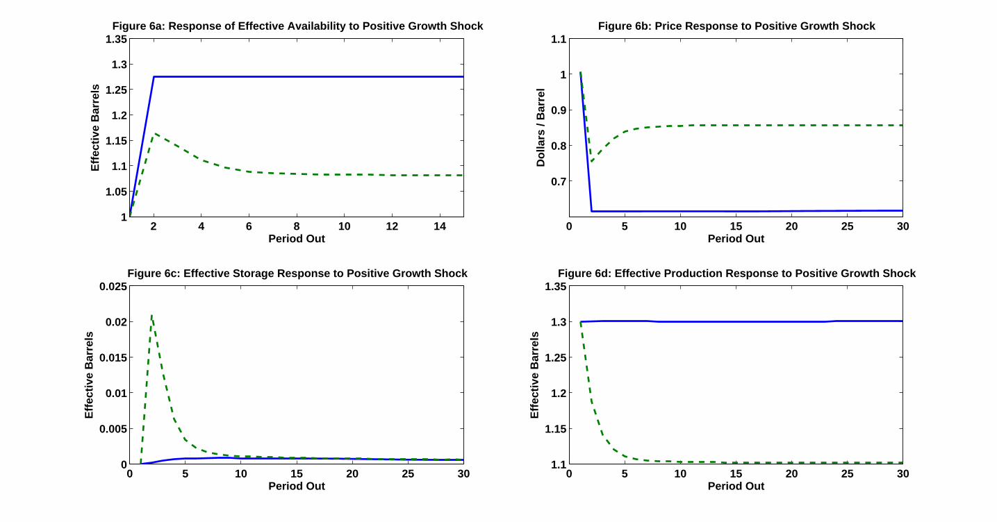
2 4 6 8 10 12 141

1.05

1.1

1.15

1.2

1.25

1.3

1.35

Period Out

Eff

ecti

ve B

arre

ls

Figure 6a: Response of Effective Availability to Positive Growth Shock

0 5 10 15 20 25 30

0.7

0.8

0.9

1

1.1

Period Out

Do

llars

/ B

arre

l

Figure 6b: Price Response to Positive Growth Shock

0 5 10 15 20 25 300

0.005

0.01

0.015

0.02

0.025

Period Out

Eff

ecti

ve B

arre

ls

Figure 6c: Effective Storage Response to Positive Growth Shock

0 5 10 15 20 25 301.1

1.15

1.2

1.25

1.3

1.35

Period Out

Eff

ecti

ve B

arre

ls

Figure 6d: Effective Production Response to Positive Growth Shock

2 4 6 8 10 12 141

1.05

1.1

1.15

1.2

Period Out

Eff

ecti

ve B

arre

ls

Figure 7a: Response of Effective Availability to Positive Growth Shock

2 4 6 8 10 12 140.7

0.75

0.8

0.85

0.9

0.95

1

1.05

Period Out

Do

llars

/ B

arre

l

Figure 7b: Price Response to Positive Growth Shock

2 4 6 8 10 12 140

0.005

0.01

0.015

0.02

0.025

Period Out

Eff

ecti

ve B

arre

ls

Figure 7c: Effective Storage Response to Positive Growth Shock

2 4 6 8 10 12 141.1

1.15

1.2

1.25

1.3

1.35

Period Out

Eff

ecti

ve B

arre

ls

Figure7d: Effective Production Response to Positive Growth Shock

StorageNo Storage

1 2 3 4 5 6 7 8 9 100.012

0.014

0.016

0.018

0.02

0.022

0.024

0.026

0.028

Periods Out

Vo

lati

lity

Figure 8: Price Volatility Following a Positive Growth Shock

Storage AllowedNo Storage