Embed Size (px)
Citation preview
Open Research OnlineThe Open University’s repository of research publicationsand other research outputs
The atmospheric circulation and dust activity indifferent orbital epochs on MarsJournal ItemHow to cite:
Newman, Claire E.; Lewis, Stephen R. and Read, Peter L. (2005). The atmospheric circulation and dustactivity in different orbital epochs on Mars. Icarus, 174(1) pp. 135–160.
For guidance on citations see FAQs.
c© [not recorded]
Version: [not recorded]
Link(s) to article on publisher’s website:http://dx.doi.org/doi:10.1016/j.icarus.2004.10.023
Copyright and Moral Rights for the articles on this site are retained by the individual authors and/or other copyrightowners. For more information on Open Research Online’s data policy on reuse of materials please consult the policiespage.
oro.open.ac.uk

Newman et al., Icarus, 174 (1) 135-160, 2005 1
The atmospheric circulation and dust activity in different
orbital epochs on Mars
Claire E. Newman,a,b,∗ Stephen R. Lewis,a and Peter L. Reada
aAtmospheric, Oceanic and Planetary Physics, Department ofPhysics, University of Oxford,
∗Corresponding Author E-mail address: [email protected]
Clarendon Laboratory, Parks Road, Oxford, OX1 3PU, United Kingdom
bDivision of Geological and Planetary Sciences, CaliforniaInstitute of Technology, Pasadena, CA 91125, USA

Newman et al., Icarus, 174 (1) 135-160, 2005 2
ABSTRACT
A general circulation model is used to evaluate changes to the circulation and dust transport in the
Martian atmosphere for a range of past orbital conditions. Adust transport scheme, including parameterized
dust lifting, is incorporated within the model to enable passive or radiatively active dust transport. The focus
is on changes which relate to surface features, as these may potentially be verified by observations.
Obliquity variations have the largest impact, as they affect the latitudinal distribution of solar heating.
At low obliquities permanent CO2 ice caps form at both poles, lowering mean surface pressures. At higher
obliquities, solar insolation peaks at higher summer latitudes near solstice, producing a stronger, broader
meridional circulation and a larger seasonal CO2 ice cap in winter. Near-surface winds associated with the
main meridional circulation intensify and extend polewards, with changes in cap edge position also affecting
the flow. Hence the model predicts significant changes in surface wind directions as well as magnitudes.
Dust lifting by wind stress increases with obliquity as the meridional circulation and associated near-surface
winds strengthen. If active dust transport is used, then lifting rates increase further in response to the larger
atmospheric dust opacities (hence circulation) produced.Dust lifting by dust devils increases more gradually
with obliquity, having a weaker link to the meridional circulation.
The primary effect of varying eccentricity is to change the impact of varying the areocentric longitude of
perihelion,l, which determines when the solar forcing is strongest. The atmospheric circulation is stronger
whenl aligns with solstice rather than equinox, and there is also abias from the Martian topography, resulting
in the strongest circulations when perihelion is at northern winter solstice.
Net dust accumulation depends on both lifting and deposition. Dust which has been well mixed within
the atmosphere is deposited preferentially over high topography. For wind stress lifting, the combination
produces peak net removal within western boundary currentsand southern mid-latitude bands, and net accu-
mulation concentrated in Arabia and Tharsis. In active dusttransport experiments, dust is also scoured from
northern mid-latitudes during winter, further confining peak accumulation to equatorial regions. As obliq-
uity increases, polar accumulation rates increase for windstress lifting and are largest for high eccentricities
when perihelion occurs during northern winter. For dust devil lifting, polar accumulation rates increase
(though less rapidly) with obliquity aboveo=25◦, but increase with decreasing obliquity below this, thus
polar dust accumulation at low obliquities may be increasingly due to dust lifted by dust devils. For all cases
discussed, the pole receiving most dust shifts from north tosouth as obliquity is increased.
Key Words: Mars, atmosphere; Mars, climate.

Newman et al., Icarus, 174 (1) 135-160, 2005 3
1 Introduction
1.1 Motivation
The current state of the Martian atmosphere has provided a challenge to atmospheric modelers, largely
because of the importance of atmospheric dust in determining weather and climate. At certain times of year
the dust loading and distribution varies greatly from day today and between years, producing an atmospheric
state which, being strongly dependent on this distribution, is also highly variable. The aim is to produce
a model which captures a statistically reasonable population of dust storms (as for the Earth, predicting
weather phenomena exactly is dependent on the quality of theinitial conditions used) and the correct amount
of interannual variability. Although progress has been made in using models to study the evolution of dust
storms (e.g. Murphy et al. 1995) and in simulating realisticdust storms and cycles with some spontaneous
variability (Newman et al. 2002a, 2002b; Basu et al. 2004), many aspects are still uncertain, for example the
dust particle size distributions, major source regions andstorm decay mechanisms.
Given these difficulties in simulating the current Martian climate, simulating the past climate (with no
direct observations and thus apparently fewer constraintson the models) may appear an impossible task. A
useful approach is to direct the modeling effort towards understanding some of the observed surface features
which change over long time scales. Certain surface features of aeolian origin (produced by the wind), for
example, indicate a preferred wind direction other than that currently found, suggesting they were formed
during an epoch when dominant wind directions differed (seee.g. Greeley et al. 2002). This suggests using a
model to determine which orbital parameters or other factors might have produced such a difference. Regions
are observed on Mars which appear to consist of long term dustdeposits (e.g. Mellon et al. 2000; Ruff and
Christensen 2002), and the ages and thicknesses of these deposits have been estimated (e.g. Christensen
1986). Here the model may be used to estimate both when these regions would last have been eroded, and
to predict net accumulation rates for different epochs.
Of particular interest are the polar layered terrains (PLTs), 10-50 m thick layers of dust and water ice
which exist polewards of∼80◦. In the north the PLT is 4-5 km deep and mostly covered by the residual
cap; in the south the PLT is 1-2 km deep and the residual cap, which is off center, covers little – the layered
terrain also extends to∼73◦S in one quadrant around∼180◦longitude. The organization of the layers has
been related to orbital variations of Mars (Toon et al. 1980;Pollack and Toon 1982; Laskar et al. 2002),
which would have affected atmospheric heating, transport,dustiness and humidity, and hence the relative
Newman et al., Icarus, 174 (1) 135-160, 2005 4
rates of water ice and dust deposition and erosion in the polar regions. A full explanation of the PLT’s
formation requires more complex models which, for example,transport both dust and water, and model the
nucleation of water ice onto dust which will clearly affect deposition rates. The polar accumulation rates in
the absence of water shown here are, however, a necessary first step.
1.2 Orbital changes over the past few million years
Mars currently has a quite eccentric orbit (eccentricitye = (a − p)/(a + p) =0.0934, wherea is
the aphelion distance andp the perihelion distance between Mars and the Sun), meaning that at perihelion
Mars receives roughly a third more solar insolation than at aphelion. Mars has a planetary obliquityo
(angle between the spin axis of the planet and the normal to the orbit plane) of 25.19◦, similar to that of
the Earth (23.5◦). Perihelion occurs at an areocentric longitude (Ls) corresponding to late northern fall
– the areocentric longitude of perihelion,l, is 251◦ (with northern spring equinox, summer solstice, fall
equinox and winter solstice occurring at Ls= 0◦, 90◦, 180◦ and 270◦ respectively). Over tens of thousands
of years these parameters vary, due to perturbations by other bodies in the solar system and the precession
and obliquity variations of Mars’s spin axis (Ward 1992; Touma and Wisdom 1993).
Recent work carried out to estimate past variations is expected to be accurate back to roughly 10 Myrs in
the past, beyond which point chaotic behavior in the solution becomes significant (Laskar et al. 2002), and
may be summarised as follows. The largest variations ine are due to a large amplitude modulating envelope
with a period of 2.4 Myrs. The large amplitude variations areas much as 0.115 (frome ∼0 to e ∼0.115),
with smaller, higher frequency (95,000–99,000 yrs) changes typically one third as large. The main period in
o is about 120,000 yrs, modulated on an∼1Myr timescale. Over about the past 4 Myrso has varied between
∼15◦ and 35◦, though from∼5–10Myrs agoo varied between∼25◦ and 45◦. Finally, l precesses with a
period of about 50,000 yrs.
1.3 The experiments
The experiments are summarized in table 1. The first experiments presented here (o15PAS, presPAS,
o35PAS and o45PAS, section 3) simulate the changes in atmospheric circulation and dust transport produced
in a Mars general circulation model (MGCM, see section 2) when obliquity is varied from 15◦ to 45◦ in
steps of 10◦. Here dust transport includes atmospheric advection by model winds, atmospheric mixing by
vertical diffusion and convective adjustment, gravitational sedimentation of dust through the atmosphere,

Newman et al., Icarus, 174 (1) 135-160, 2005 5
Table 1: The experiments and parameter values used
Name Obliquity Eccentricity Longitude of Passive or αN αD
o (in ◦) e perihelionl (in ◦) active dust (m−1) (kg J−1)o15PAS 15 current current passive 1.3×10⁻⁵ 1.6×10⁻⁹
presPAS current current current passive 1.3×10⁻⁵ 1.6×10⁻⁹
o35PAS 35 current current passive 1.3×10⁻⁵ 1.6×10⁻⁹
o45PAS 45 current current passive 1.3×10⁻⁵ 1.6×10⁻⁹
presAC current current current active 2.25×10⁻⁶ –o35AC 35 current current active 2.25×10⁻⁶ –e0PAS current 0 current passive 1.3×10⁻⁵ 1.6×10⁻⁹
l71PAS current current 71 passive 1.3×10⁻⁵ 1.6×10⁻⁹
l180PAS current current 180 passive 1.3×10⁻⁵ 1.6×10⁻⁹
and injection from the surface via a near-surface wind stress or dust devil lifting parameterization. The dust
distribution predicted by the dust transport scheme has no impact on the atmospheric state in these passive
runs, but the lifting parameter (αN or αD, see section 2.1) for current orbital conditions is still chosen
to provide a reasonable match between simulated and currently observed typical dust opacities. This is
necessary to estimate the rate of accumulation of surface dust, which also depends on atmospheric transport
and dust deposition. For consistency, the same lifting parameter is then used for all passive dust simulations,
regardless of the orbital configuration. As discussed above, atmospheric dustiness plays a large part in
determining the model state, but for these initial experiments a prescribed dust distribution is presented to
the MGCM’s radiative transfer routine which has a simple spatial variation and is constant in time (in terms
of dust mixing ratios, see section 2.1). This will of course produce strictly inaccurate results, as the total dust
load and its spatial distribution actually vary through theyear on Mars itself. A variable dust distribution
could be prescribed for the current epoch, based on observations, but this would also bias results if used
without alteration for other orbital settings.
This problem motivated the running of two active simulations for which the dust distributions are pro-
duced by the simulations themselves, using the wind stress dust lifting parameterization only and radiatively
active dust transport (presAC and o35AC, section 4). This allows feedbacks between the circulation, dust
transport within the atmosphere and dust lifting from the surface. The dust lifting parameterization is tuned
to provide a reasonable match to currently observed Mars years without large dust storms foro=25◦, and
again for consistency is then applied without change too=35◦.
In section 5 the effects of changing eccentricity and time ofperihelion are also considered for the present
obliquity. First the eccentricity is set to the minimum value possible,e=0, giving a circular orbit which results

Newman et al., Icarus, 174 (1) 135-160, 2005 6
in the same total insolation being incident on Mars throughout the year (e0PAS). Two further experiments
examine the impact of perihelion occurring shortly before summer solstice in the northern rather than the
southern hemisphere (l=71◦, l71PAS), and occurring at northern fall equinox (l=180◦, l180PAS), for the cur-
rent eccentricity. Biases towards a stronger circulation during northern winter in each of these experiments
are also investigated and discussed.
2 The model and dust lifting parameterizations
2.1 Description
The model used for this work is the Oxford version of the Mars general circulation model developed
jointly at the sub-department of Atmospheric, Oceanic and Planetary Physics at the University of Oxford
and the Laboratoire de Meteorologie Dynamique du Centre National de la Recherche Scientifique in Paris.
The model used here (the MGCM) is almost identical to the Oxford version described in Forget et al. (1999),
though with some changes including a different formulationof the radiative transfer code. Unless otherwise
specified it is run at relatively low horizontal resolution (spectral truncation T21, with dust stored on a 7.5◦×
7.5◦ grid). The vertical resolution used is as in Lewis et al. (1999), with the lowest level at∼5m, levels
closely spaced through the boundary layer, and 25 levels in all up to ∼90km. The MGCM used here also
includes the dust transport scheme described in Newman et al. (2002a, 2002b), though with near-surface
wind stresses now calculated after the vertical diffusion scheme is applied to the model wind field, giving
generally lower values; it does not include transport of water vapor and water ice particles.
In the experiments shown here the dust transport scheme was run using a single dust particle size of 1µm
radius, with dust as either a passive or an active tracer. In the latter case the MGCM’s radiation code sees the
changes to the atmospheric dust distribution which are simulated by the scheme, and responds accordingly,
using radiative dust properties representative of the observed size distribution (rather than 1µm particles). In
the former case the radiation code sees a prescribed dust distribution, and in the passive dust experiments
shown here a moderate background level of dust loading is used. Visible dust opacity referenced to the
700Pa pressure surface is 0.2 at all times and locations, with the vertical distribution given by
q = q0 exp{
0.007[
1 − (p0/p)(70km/zmax )]}
, (1)
whereq=mass mixing ratio,q0=a reference value which results in the required dust opacity (0.2 at 700Pa

Newman et al., Icarus, 174 (1) 135-160, 2005 7
here),p andp0 are pressure and reference pressure (700Pa here) respectively, andzmax=30km (this is low
for times of strong dust activity, but probably higher than during the clearest periods). As shown in Fig. 3 of
Lewis et al. (1999), this produces a sharp exponential decline in dustiness to the dust top height ofzmax.
The lifting parameterizations used are similar to some of those described in Newman et al. (2002a).
Lifting by near-surface wind stressζ is modeled using a slightly simpler method than in Newman et al.
(2002a), which required three parameters to be specified andcalculated threshold wind stresses at each
gridpoint and time. Here dust is lifted when a constant threshold wind stressζt is exceeded (here 0.01N/m2),
with the lifted dust flux given by
αN × 2.61ζ3/2
g√
ρ
(
1 −
√
ζt
ζ
)(
1 +
√
ζt
ζ
)2
, (2)
whereg=gravitational acceleration andρ=near-surface atmospheric density. Thus only two parameters
are involved (ζt, andαN which determines the actual amounts lifted). Although the same threshold stress
is used in all experiments shown in table 1, it would be unphysical to apply the same value ofαN to both
passive and active dust simulations. The active dust runs (which include the impact of dust on the Martian
climate, hence are more realistic) allow strong positive feedbacks between dust loading, circulation strength
and further lifting, and therefore produce far higher peak opacities than produced by passive simulations for
the same value ofαN (Newman et al. 2002b). The value ofαN is therefore chosen to be 1.3×10⁻⁵ m−1 for
all passive dust simulations, and 2.25×10⁻⁶ m−1 (almost 6 times smaller) for all active dust simulations.
In both cases it is chosen to produce peak zonally averaged, visible atmospheric dust opacities of∼1 in
northern low latitudes for the two simulations run using present day orbital settings (presPAS and presAC),
in line with peak visible opacities observed or inferred fora typical Mars year (Clancy et al. 2000; Smith et
al. 2001; Liu et al. 2003; Smith 2004).
Lifting by dust devils is set proportional to the ‘dust devilactivity’, with constant of proportionality
αD. The dust devil activity is a measure of how much energy is available to drive the dust devils, defined
by Renno et al. (1998) as roughly the thermodynamic efficiency of the dust devil convective heat engine
multiplied by the surface sensible heat flux. The former increases with convective boundary layer height,
while the latter is the heat input to the base of the dust devil, which is positive if the surface temperature
exceeds that of the atmosphere above it. Lifting by dust devils may be ubiquitous (e.g. Edgett and Malin
2000) and may contribute to a large fraction of the dust lifted (Ferri et al. 2003; Basu et al. 2004), except
during the storm season when wind stress lifting probably dominates in producing any large dust storm

Newman et al., Icarus, 174 (1) 135-160, 2005 8
events (Cantor et al. 2001; Newman et al. 2002b; Basu et al. 2004). Using a value ofαD=1.6×10⁻⁹ kg J−1,
which produces peak opacities of∼1 during the storm season for the present orbital settings, may therefore
overestimate the amount of dust devil lifting at this time ofyear in particular, but is used to calculate dust
devil lifting in the passive dust experiments for comparison with the wind stress lifting results. Experiments
with both lifting mechanisms and active dust transport are an obvious next step, following on from the active
dust simulations with wind stress lifting shown in section 4, but were not included in this initial work as they
greatly increase the sensitivity of results to the parameters chosen and hence the complexity of analysis.
2.2 Performance of the lifting parameterizations for current orbital settings
2.2.1 Comparison with observations
It is important to assess the performance of the dust liftingparameterizations for the present epoch
before proceeding. Wind stress lifting is thought to be dominant in producing dust storms, thus predicted
wind stress lifting sites can be compared with observed initiation regions of large dust storms observed
between Ls=120◦ and Ls=270◦ during the first year of Mars Global Surveyor (MGS) observations. Figure 1
shows plots of the annual thickness of dust lifted for five shorter periods, then for the entire longer period,
as predicted by a present day simulation which used radiatively active dust transport with wind stress lifting
only (experiment presAC). The lifted dust flux (from equation 2) is converted to dust thickness by assuming
a dust density of 2500kg m−3. Superimposed on this are asterisks marking storm initiation sites extracted
from Mars Orbiter Camera (MOC) images (Cantor et al. 2001). Haberle et al. (2003) performed a similar
comparison between lifting predicted by the NASA Ames Mars general circulation model and MOC storm
observations. They defined ‘deflation potential’ as the thickness of dust which would be removed over a
given period of time (typically 1 year), but used a simpler formula to calculate the lifted dust flux. They
also used a larger threshold stress than used in the MGCM (0.02Nm−2), which reflects the fact that MGCM
surface winds are generally slightly lower in magnitude than those produced by the model of Haberle et al.
(2003).
Looking at the final plot for the entire period, there are regions of good agreement between MGCM
predictions and MOC observations. In particular, the modelpredicts the lifting observed to the east of the
highlands of Tharsis, Syrtis and Elysium. These locations experience enhanced meridional flows known as
western boundary currents (WBCs, see e.g. Joshi et al. 1995). The clear regions between these positions in
the range∼60◦N to 20◦S coincide in the model and observations. From Ls=240◦–270◦, the MGCM predicts

Newman et al., Icarus, 174 (1) 135-160, 2005 9
Ls 120-150 degrees
-180 -120 -60 0 60 120 180-90
-60
-30
0
30
60
90
La
titu
de
*
*
*** * *** *
*
** * ** ***
*
*
*
*
*
*** *
*
**
*** *
*
**
** ** **
***
**
*
Ls 150-180 degrees
-180 -120 -60 0 60 120 180-90
-60
-30
0
30
60
90
*
*
***** ***
* *
* *
***
*
**
*
**
***
*
* *
*
* ** *
*
*
*
***
** ** ***
*
****
*
* * **
*
* * **
** ** * ****
* *
* ** *
** **
***
***
*
* **** * *
***
* **
*
**
* ** ***
* *
** *
* *
*
**
*
**
***
*
* *
*
* ****
*** *
*
**
* **** *
*
** *
*
**
** ** ****
* *
*
** *
*
*
***
**** ****
*
***
**
** **
*
*
*
*
**
* * ** * *
*
* *** *
**
**
*
*
******* *
**
**
**
***
**
*
* *****
**
*
**
**
*
**
**
* *
*
* ***
** *** **** ****
*
***
*
**
Ls 180-210 degrees
-180 -120 -60 0 60 120 180-90
-60
-30
0
30
60
90
La
titu
de
10-4
10-4
10-4
10-2
10
-2
* * ** *
*
*
*
**
****
*
** *
*
***
*
**
* *
*
* * ***
*
*
*
* **
*
**
**
*
***
**
***
****
***
*
*
*
***
*
*
*
** *
*
*
**
**
*
******
* **
*
*
*
*
*
*
*
*
****
** * **
*
***
***
*
*
*
*
*
*** **
*
**
* ****
*
**
**
*
*
*
* **
**
* ** * *
**
*
* *
*
**
*
**
* *
*
*
* **
** *
* * *
*
*
*
*
**
*
****** *
**
*
Ls 210-240 degrees
-180 -120 -60 0 60 120 180-90
-60
-30
0
30
60
90
10-410-2
* *
*
*
**
* *
** * *
* ***
** *
*
*** **
*
**
*
****
***
*
*
**
***
* ***
** **
*
***
*** *
**
**
* ***
**** ** *
* ***** *
* ** ***
**
** *
**
*** **
**
**
*
**
**
*
**
***** **
**
** ***
*
***
* ** *
*
* * ****
*****
*****
* ** **
* ***
**** *
***
**
*
***
*
*
***
*
* *
***
**
*
*
*
*
*
*
*
**
**
* *
*
*
**
**
*
** **
**
*
**
*** **
* *
*
** * * * *** ** **
Ls 240-270 degrees
-180 -120 -60 0 60 120 180Longitude
-90
-60
-30
0
30
60
90
La
titu
de
10-4
10-4
10-4 *
*
* **
*
**** **
*
** ***
*
** **** * *** ****
* *** * **
Ls 120-270 degrees
-180 -120 -60 0 60 120 180Longitude
-90
-60
-30
0
30
60
90
10-4
10-41
0-4
10-4
10-4
10-4
10-2
10
-2
10-2
*
*
*** * *** *
*
** * ** ***
*
*
*
*
*
*** *
*
**
*** *
*
**
** ** **
***
**
**
*
***** ***
* *
* *
***
*
**
*
**
***
*
* *
*
* ** *
*
*
*
***
** ** ***
*
****
*
* * **
*
* * **
** ** * ****
* *
* ** *
** **
***
***
*
* **** * *
***
* **
*
**
* ** ***
* *
** *
* *
*
**
*
**
***
*
* *
*
* ****
*** *
*
**
* **** *
*
** *
*
**
** ** ****
* *
*
** *
*
*
***
**** ****
*
***
**
** **
*
*
*
*
**
* * ** * *
*
* *** *
**
**
*
*
******* *
**
**
**
***
**
*
* *****
**
*
**
**
*
**
**
* *
*
* ***
** *** **** ****
*
***
*
** * * ** *
*
*
*
**
****
*
** *
*
***
*
**
* *
*
* * ***
*
*
*
* **
*
**
**
*
***
**
***
****
***
*
*
*
***
*
*
*
** *
*
*
**
**
*
******
* **
*
*
*
*
*
*
*
*
****
** * **
*
***
***
*
*
*
*
*
*** **
*
**
* ****
*
**
**
*
*
*
* **
**
* ** * *
**
*
* *
*
**
*
**
* *
*
*
* **
** *
* * *
*
*
*
*
**
*
****** *
**
* * *
*
*
**
* *
** * *
* ***
** *
*
*** **
*
**
*
****
***
*
*
**
***
* ***
** **
*
***
*** *
**
**
* ***
**** ** *
* ***** *
* ** ***
**
** *
**
*** **
**
**
*
**
**
*
**
***** **
**
** ***
*
***
* ** *
*
* * ****
*****
*****
* ** **
* ***
**** *
***
**
*
***
*
*
***
*
* *
***
**
*
*
*
*
*
*
*
**
**
* *
*
*
**
**
*
** **
**
*
**
*** **
* *
*
** * * * *** ** **
**
* **
*
**** **
*
** ***
*
** **** * *** ****
* *** * **
Figure 1: Newman et al. Predicted wind stress lifting and MOCstorms observed.

Newman et al., Icarus, 174 (1) 135-160, 2005 10
far more lifting than suggested by observations of initial dust clouds, in the region∼25◦–35◦S where strong
north-westerlies associated with the zonal mean circulation are produced. However, elevated dust levels due
to regional storms in the period Ls∼230◦–270◦ may have obscured individual lifting events.
The MGCM captures some (though not all) of the band of liftingin southern spring-summer which
moves polewards with time. This movement suggests it is at least partly due to strong near-surface winds
near the retreating polar cap edge, a region of strong temperature gradients giving rise to thermal contrast
and baroclinic flows, which the MGCM models as retreating at just such a rate. Interestingly, the passive
dust simulation (presPAS) does not predict as much lifting within this band, particularly as the band moves
to higher latitudes, suggesting that the atmospheric dust distribution (and its effect on surface winds) in the
active case is more realistic than in the passive case (wherea more uniform prescribed distribution is used in
the radiative transfer scheme). The best match between observed and predicted cap edge lifting occurs when
strong cap edge flows are combined with slope winds in the Hellas and Argyre basins. The lack of lifting
at other longitudes along the receding cap edge may be due to the precise choice of lifting threshold, or the
low model resolution may prevent the model from resolving small scale thermal contrast flows, slope winds
and/or wave activity. A similar lack of lifting early on in northern polar regions may be due to the MGCM
having no water ice cap, hence cap edge flows only become possible when the seasonal CO2 ice cap begins
to form in late fall.
Mapping of dust devil activity observed on Mars is still underway, making it difficult to assess conclu-
sively the performance of the lifting parameterization used here, although it has been shown to be consistent
with what observations are currently available (Newman et al. 2002a). A comparison with the observations
of initial storm clouds shown in Fig. 1 is probably inappropriate, given that observations show no correlation
between dust devils and storm initiation (Cantor et al. 2001), and that simulations which assume dust devils
to be the primary lifting mechanism for Mars produce far morelifting (and consequently far higher dust
opacities than observed) during northern spring and summer(Newman et al. 2002b). Fig. 7 (discussed in
section 3.2.2) includes a plot showing regions of peak dust devil lifting for the current epoch, and as expected
these do not match the observations shown in Fig. 1.
2.2.2 Dust lifting rates and the benefits of a dust transport scheme
In terms of patterns of wind stress lifting there is reasonable agreement between the results shown in the
final plot of Fig. 1 and those shown in figure 4 of Haberle et al. (2003). There are significant differences,

Newman et al., Icarus, 174 (1) 135-160, 2005 11
however, in the amount of lifting predicted. Foro=25◦, for example, the MGCM predicts just under 0.01cm
of dust lifted per year in peak lifting regions, whereas Haberle et al. (2003) find a peak deflation potential
greater than 10cm per year. Haberle et al. (2003) do not include dust transport in the version of their model
used to calculate deflation potential, but these results suggest that, were they to do so, their higher lifting
rates would probably produce orders of magnitude higher (and thus unrealistic) atmospheric dust opacities
than produced by the MGCM. This emphasizes the usefulness ofincluding dust transport schemes within
Mars models if quantitative estimates of dust lifting rates(hence also deposition and net accumulation rates)
are of interest, as this allows the lifting parameter (hereαN) to be chosen on the basis of producing realistic
atmospheric opacities. Results using the GFDL Mars model (Basu et al. 2004), which also tunes the dust
injection to produce realistic opacities, support the smaller deflation potentials predicted by the MGCM.
3 The effect of varying obliquity using passive dust transport
3.1 The atmospheric circulation
This has already been discussed in detail by previous authors (Fenton and Richardson 2001; Haberle et
al. 2003; Mischna et al. 2003) so the current section gives only a brief overview of the main results, followed
by a description of selected points including the main differences found between this and previous work.
3.1.1 Overview
The basic idea is that changing a planet’s obliquity alters the distribution of solar heating across its
surface. For Mars, with a primarily CO2 atmosphere, the major effect is on the formation / removal of
CO2 surface ice. At low obliquities the poles never receive muchsolar insolation, resulting in a lowering
of their annual mean surface temperatures and hence a CO2 ice build-up. Below some critical obliquity,
between 15◦ and 25◦ in the MGCM and∼21.6◦ in the energy balance model of Fanale and Salvail (1994),
permanent CO2 ice caps therefore exist at both poles. At high obliquities,the polar regions receive far more
solar insolation during summer and less during winter, hence the summer pole is free of CO2 ice but large
seasonal CO2 caps form at the winter pole. This results in an increase in the amplitude of the annual pressure
cycle (which for all obliquities has peaks in early northernand southern summer, when the summer seasonal
cap has largely sublimed but the winter cap is still midway through forming). Plots of globally averaged
surface temperature in the MGCM are similar to those shown inFig. 5 of Haberle et al. (2003). Plots of
Newman et al., Icarus, 174 (1) 135-160, 2005 12
Obliquity = 15 degrees
0 30 60 90 120 150 180 210 240 270 300 330 0-90
-60
-30
0
30
60
90
Latit
ude
155
155
170
170
185
185
200
200
215
215
230
Obliquity = 25 degrees
0 30 60 90 120 150 180 210 240 270 300 330 0Areocentric longitude Ls
-90
-60
-30
0
30
60
90
155
155 155
170
170
170
185
185
185
185
200
200
200
200
215 215
215
215
230
245
Obliquity = 45 degrees
0 30 60 90 120 150 180 210 240 270 300 330 0Areocentric longitude Ls
-90
-60
-30
0
30
60
90
Latit
ude
155
155
155
170
170
170
185
185
185200
200
200
200
215
215
215
215
230
230
245
245
260
26027
5
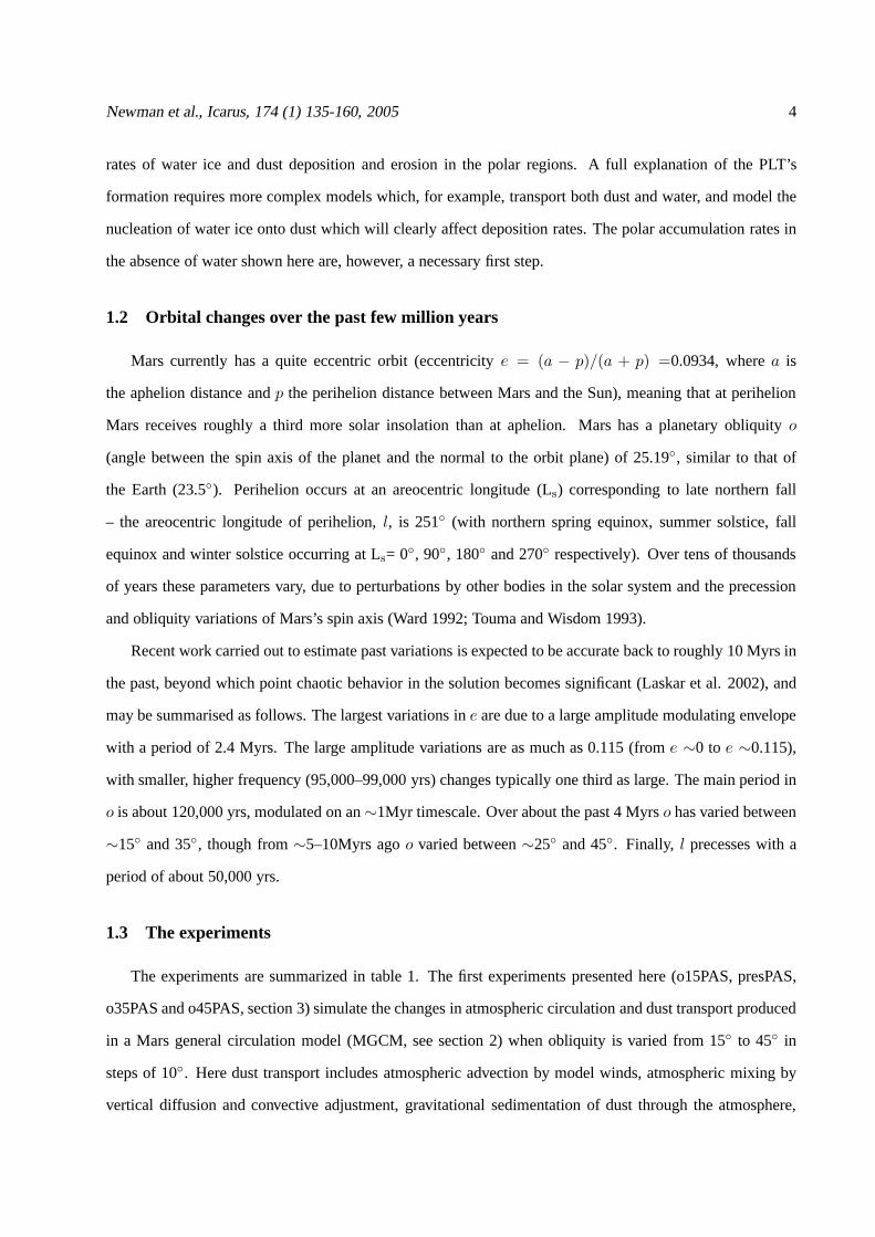
Figure 2: Newman et al. Zonal mean surface temperature and CO2 ice cap edge.
globally integrated atmospheric mass are very similar to those shown in Fig. 1 (giving results only foro=25◦
and higher) of Mischna et al. (2003). Equivalent plots of globally averaged surface pressure are very similar
to results foro=25◦ and higher shown in Fig. 8 of Haberle et al. (2003), although differ from the latter for
lower obliquities due to the effect on surface pressure of polar ice accumulation in the MGCM (see section
3.1.2).
Figure 2 demonstrates the effect of varying obliquity on surface temperatures and CO2 ice cover, and is
similar to Fig. 6 of Haberle et al. (2003) except that the cap edge is defined here as the latitude at which the
zonal mean CO2 ice cover exceeds 1kg m−2 (rather than as the latitude for which one or more grid points
has ice cover, as in Haberle et al. (2003), which would tend tomake the caps appear larger than shown
here). As obliquity increases, peak surface temperatures move to higher summer latitudes, and in the winter
hemisphere the seasonal CO2 cap reaches to lower latitudes (though never reaches the equator, except at a
few longitudes foro=45◦) thus pinning surface temperatures at the CO2 frost point (∼150K) over much of
the planet. Except for a ‘bunching up’ of temperature contours at the edge of increasingly large residual caps
(and colder surface temperatures at latitudes where the capis present at one obliquity but not at another),
equinoctial surface temperatures vary little with obliquity.
The stepped nature of the zonal mean cap edge position shown in Fig. 2 is due to the fact that entire
gridpoints are cleared of / gain ice cover at a time, rather than this happening smoothly and incrementally as

Newman et al., Icarus, 174 (1) 135-160, 2005 13
on Mars itself. This also affects the zonal mean surface temperatures (and low level atmospheric tempera-
tures, not shown) at the receding cap edge, where removal of ice from an entire gridpoint allows the surface
to warm rapidly from the CO2 frost point to temperatures representative of ice-free regolith. The reverse
effect does not occur during cap formation, as at this time the surrounding atmosphere cools beforehand,
buffering the effect. The step sizes are related to the grid resolution used, thus MGCM simulations run at
higher resolution show a smoother variation in cap edge surface temperatures. Similar step features occur
in plots of global mean surface temperature predicted by theMGCM, and are very nearly identical to those
shown in Fig. 5 of Haberle et al. (2003), since both models used comparable horizontal resolution.
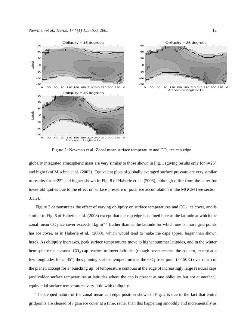
Figure 3 shows the effect of increasing obliquity on zonal mean zonal winds and temperatures, and
the meridional transport circulation (here given approximately by the residual mean circulation, see e.g.
Andrews et al. [1987]). The left-hand column shows the current circulation predicted by the MGCM in
northern winter using the moderate dust distribution described in section 2.1. Near both solstices a cross-
equatorial Hadley circulation dominates, with the position of the rising branch in the summer hemisphere
being linked to the latitude of maximum time-integrated solar heating. As obliquity is increased (right-hand
column), the subsolar latitude increases, as does the fraction of each latitude circle in the summer hemisphere
which receives solar insolation at any given time (though ofcourse this fraction never exceeds one, hence
once this is reached no further increase is possible). The net result is that the rising branch shifts to higher
latitudes as obliquity increases. Angular momentum constraints allow the entire Hadley cell to broaden,
increasing downwelling over the winter pole and hence the amount of polar warming produced and strength
of the circumpolar vortex. The meridional circulation alsostrengthens, with the stronger cross-equatorial
flow producing larger easterlies aloft.
At equinox (not shown) there is little difference between results for different obliquities. In both cases
the mean meridional circulation consists of two Hadley cells rising near the equator and extending only to
∼40◦, with far lower flow velocities than are encountered near solstice.
3.1.2 The impact on mean surface pressure at low obliquities
The removal of atmospheric CO2 as surface ice results in a reduction of atmospheric pressure, if the
total amount of CO2 present remains constant (as is assumed in the MGCM). The MGCM does not currently
consider other CO2 reservoirs, such as CO2 in the high latitude regolith (Toon et al. 1980; Pollack and Toon
1982). At current surface pressures a decrease in high-latitude temperatures (at low obliquities) would tend
Newman et al., Icarus, 174 (1) 135-160, 2005 14
u; obliquity 25 degrees
-90 -60 -30 0 30 60 900
20
40
60
Pseu
do-h
eigh
t abo
ve g
eoid
in k
m
-60 -20
-20
20
20
60
60
u; obliquity 45 degrees
-90 -60 -30 0 30 60 900
20
40
60
-100
-60
-20
-20
20
20
60
T; obliquity 25 degrees
-90 -60 -30 0 30 60 90Latitude in degrees
0
20
40
60
Pseu
do-h
eigh
t abo
ve g
eoid
in k
m
150
150
170
170
170
190210230
T; obliquity 45 degrees
-90 -60 -30 0 30 60 90Latitude in degrees
0
20
40
60
150
150
150
150
170
170
170
190
210230
Figure 3: Newman et al. The zonal mean northern winter solstice circulation foro=25◦and 45◦.
to increase CO2 adsorption rates, although the reduction in surface pressure due to increased cap deposition
would tend to produce the opposite effect and reduce adsorption rates, actually releasing more CO2 again
(Fanale and Salvail 1994). Most of any additional CO2 released would likely condense onto the caps,
however, so surface pressure estimated neglecting the regolith adsorption may be approximately correct,
although the amount of ice formed is probably an underestimate.
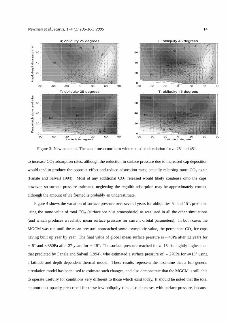
Figure 4 shows the variation of surface pressure over several years for obliquities 5◦ and 15◦, predicted
using the same value of total CO2 (surface ice plus atmospheric) as was used in all the other simulations
(and which produces a realistic mean surface pressure for current orbital parameters). In both cases the
MGCM was run until the mean pressure approached some asymptotic value, the permanent CO2 ice caps
having built up year by year. The final value of global mean surface pressure is∼40Pa after 12 years for
o=5◦ and∼350Pa after 27 years foro=15◦. The surface pressure reached foro=15◦ is slightly higher than
that predicted by Fanale and Salvail (1994), who estimated asurface pressure of∼ 270Pa foro=15◦ using
a latitude and depth dependent thermal model. These resultsrepresent the first time that a full general
circulation model has been used to estimate such changes, and also demonstrate that the MGCM is still able
to operate usefully for conditions very different to those which exist today. It should be noted that the total
column dust opacity prescribed for these low obliquity runsalso decreases with surface pressure, because

Newman et al., Icarus, 174 (1) 135-160, 2005 15
Obliquity = 5 degrees
0 1 2 3 4 5 6 7 8 9 10 11 12
100
200
300
400
500
600
Surf
ace p
ressure
(P
a)
Obliquity = 15 degrees
0 1 2 3 4 5 6 7 8 9 10 11 12 13 14 15 16 17 18 19 20 21 22 23 24 25 26 27Year
350
400
450
500
550
600
650
Surf
ace p
ressure
(P
a)
Figure 4: Newman et al. Surface pressure for 5 and 15◦ obliquity.
the dust is prescribed to have a constant opacity – but at a reference pressure of 700Pa – in all of the passive
dust experiments (see section 2.1).
Once no permanent caps exist the model of Fanale and Salvail (1994) predicts that increased summer
temperatures, tending to release more CO2 from the high latitude regolith, are balanced by the effect of
the increased surface pressures (causing the regolith to adsorb more CO2), hence resulting in little variation
in mean surface pressure at high obliquities. There may alsobe increased adsorption into the low latitude
regolith. The permanent caps disappear at an obliquity of∼32.3◦ in their model, by which point a mean
surface pressure of∼710Pa (slightly higher than the current value) has been achieved owing to the release of
CO2 from the caps. In the MGCM, by contrast, the annual mean surface pressure is slightly lower ato=35◦
and 45◦ than for the current obliquity, due to the huge seasonal capsremaining large further into spring (as
shown in Fig. 2 by the more gradual initial retreat as obliquity increases).
3.1.3 Surface wind patterns and aeolian features
The surface wind pattern is key to the formation of many surface features and to dust lifting by near-
surface wind stress. Figure 5 shows surface winds averaged over 10 sols at Ls= 90◦, 180◦ and 270◦ (northern
summer, fall and winter respectively) for three obliquities. The cross-equatorial flow at solstice – the return
branch of the Hadley circulation, which is concentrated into WBCs as discussed in section 2.2 – becomes

Newman et al., Icarus, 174 (1) 135-160, 2005 16
stronger and extends to higher summer latitudes as obliquity is increased and the Hadley circulation becomes
stronger and broader. By conservation of angular momentum,as these flows move away from the equator
they are turned towards the east, producing increasingly strong summer mid-latitude westerlies extending
to increasingly high latitudes. In the winter hemisphere, increasing coverage by the seasonal cap leads to
broad areas (those covered by the cap but away from its edge) with low surface temperature gradients, hence
limits near-surface wind magnitudes. The location of the cap edge, at which a strong thermal contrast exists,
also has a large effect. For example, during fall when local thermal contrast / topographic flows dominate
(see e.g. Siili et al. 1999), the cap edge lies across the southern slopes of the Argyre and Hellas basins at
low obliquity, hence daytime off-cap winds are in the same direction as nighttime downslope winds over
the adjacent regolith (with winds continuously downslope over icy slopes). Yet byo=45◦ the cap edge lies
across the middle of the basins, hence daytime off-cap windsand daytime upslope winds over the adjacent
regolith are in the same direction, producing even strongersurface winds further equatorwards than for the
lower obliquity. Thus the main differences in dominant surface wind velocities, due to changes in obliquity,
are predicted to occur in the mid to high latitude range affected by the change in Hadley cell and cap extent
at a particular time of year, and may include changes in direction as well as magnitude.
Fenton and Richardson (2001) concluded that surface wind directions were essentially unchanged by
variations in obliquity, but focused on changes associatedwith the Hadley circulation, and also limited their
investigation to a maximum of 35◦ obliquity. In MGCM results foro=35◦ (not shown) the expansion of the
Hadley cell at the surface is in fact quite small despite a larger expansion aloft, whereas there is significant
expansion even at the surface (as shown in Fig. 5) by 45◦. This suggests a bias towards the low level Hadley
circulation being constrained equatorwards of∼40◦S in the southern summer hemisphere, perhaps due to
the Martian topography.
The most direct way to verify these predictions would be to identify aeolian features in the same region
of Mars which show evidence of having been produced under different dominant wind regimes. For example
at∼40◦N, 40◦W, the MGCM predicts strong westerlies or west-south-westerlies ato=45◦, peaking during
northern summer, whereas for the present day it predicts that the strongest winds are north-easterlies occuring
during northern fall and winter. Similar behavior is predicted for∼40◦N, 110◦E. Ideal features would be
yardangs (streamlined features carved by wind abrasion by dust and sand, typically highest and broadest at
the blunt end that faces into the wind), ventifacts (rocks with pits, flutes and facets caused by wind abrasion,
many with the alignment of grooves and pits recording the prevailing wind direction) or dunes (whose type

Newman et al., Icarus, 174 (1) 135-160, 2005 17
Figure 5: Newman et al. Near-surface winds for three obliquities.

Newman et al., Icarus, 174 (1) 135-160, 2005 18
and shape often indicate the dominant wind direction duringformation). Wind streaks (due to either the
removal or deposition of material, generally bright dust) are less useful as they typically represent only
current wind regimes.
Unfortunately, it is difficult to observe ventifacts, yardangs and dunes in sufficient detail. Ventifacts are
too small to be observed from orbit, so can only be seen in lander images. Yardangs are larger and hence more
visible, but it is still difficult to determine the sense of prevailing winds (rather than just their orientation)
without high resolution imaging. Both the direction and sense of prevailing winds can be obtained relatively
easily from certain dune types, e.g. barchan dunes, though again this requires sufficiently high resolution
imaging of dune fields. Observations targeting aeolian features, specifically yardangs and dunes, in the
regions of interest discussed above could be used to validate the MGCM’s predictions of changes in surface
wind patterns, which would also indirectly validate its predictions of seasonal cap extent and circulation
changes for different orbital configurations.
Thus far, the Mars Pathfinder landing site (∼19.3◦N, 33.6◦W) is the only location on Mars for which
there exists strong evidence for a change in wind direction using these techniques. Dominant winds here
were inferred to be from the north-east, by observing the orientation of nearby bright features assumed to
be dunes imaged from orbit, and the direction and sense of depositional wind streaks and tails in the lee
of obstacles seen both from orbit and in Pathfinder images (e.g. Greeley et al. 1999). The MGCM, in
agreement with other Mars models (e.g. Fenton and Richardson 2001; Haberle et al. 2003), also currently
predicts dominant winds from the north-east in this region (occurring during northern winter). Yet the
Pathfinder images also show flutes and ventifacts on rocks which indicate prevailing winds from the east-
south-east (e.g. Bridges et al. 1999), raising the possibility that under different orbital conditions this might
have been the dominant wind direction (Greeley et al. 2000).Experiments conducted using the MGCM at
higher obliquities do indeed show a change in dominant wind direction here byo=45◦, due to the presence
of increasingly strong southerlies/south-westerlies in northern summer as the strength of the meridional
circulation at this time of year increases, whilst northernwinter wind magnitudes here drop due to increased
ice cover over the northern hemisphere. For sufficiently high dust levels (e.g. as in the active dust transport
experiments described in section 4) northerlies/north-easterlies during northern winter may again dominate
if the size of the seasonal cap is reduced in a warmer atmosphere. But for none of the cases described here
(including varying eccentricity and areocentric longitude of perihelion for the current obliquity, see section
5) does the MGCM predict east-south-easterlies to dominatein this region. This result is in agreement with

Newman et al., Icarus, 174 (1) 135-160, 2005 19
the findings of Fenton and Richardson (2001) and Haberle et al. (2003), and suggests a cause other than
solely variations in orbital parameters.
3.2 Dust transport
3.2.1 The latitudinal variation of dust lifting and deposition
The upper two rows in Fig. 6 show zonal mean dust lifting by near-surface wind stress (top) and dust
devils (bottom) respectively using the simple parameterizations described in section 2.1, foro=25◦ and 45◦
(experiments presPAS and o45PAS). The results were produced using passive dust transport, and for wind
stress in particular are also dependent on the choice of parameter values, but still provide insight into the
variation of dust processes with obliquity. The MGCM currently predicts little interannual variability in
dust lifting for all lifting parameters used. For high threshold wind stresses, and using radiatively active
dust transport, a small amount is produced in terms of the appearance (or not) of a cross-equatorial dust
storm (Newman et al. 2002b), but overall there is less interannual variability than observed on Mars itself.
The results shown here are therefore taken from a single year-long simulation (following an initial ‘spin-up’
year), as results are unlikely to differ significantly from averaged results of multi-year simulations.
Near-surface wind magnitudes (see section 3.1.3), wind stress and hence wind stress dust lifting greatly
increase overall with obliquity, with the latter two particularly suppressed ato=15◦ due to the reduced sur-
face pressure. Lifting peaks during northern winter for allobliquities. For high obliquities this is due to the
stronger global circulation at this time and the associatedstrong near-surface winds (peaking in the summer
hemisphere), but for low obliquities it is also due to the presence of strong baroclinic and cap edge flows
in the winter hemisphere due to strong high latitude temperature gradients in the vicinity of the winter ice
cap edge. The latter decrease in relative importance as obliquity increases (as this results in the cap edge
shifting to lower latitudes and the mean meridional circulation becoming increasingly dominant). Lifting
during northern summer becomes significant for higher obliquities, as the global mean circulation and re-
lated surface winds increase in strength, though there is still less lifting than at the opposite solstice. This
asymmetry is enhanced in active dust experiments for which positive feedbacks exist between dust amounts
and wind stress lifting (see section 4).
For all obliquities, peak dust devil lifting occurs at∼25◦ north or south during northern or southern
summer respectively, rather than following the sub-solar point (the position of peak instantaneous surface
heating) which is shifted polewards with obliquity for any given sol in summer. The reason is that heating of

Newman et al., Icarus, 174 (1) 135-160, 2005 20
Wind stress lifting, obliquity=25
0.0000
0.0005
0.0010
0.0015
0.0020
0.0025
Liftin
g (
cm
/ye
ar)
67.5-90 N45-67.5 N22.5-45 N0-22.5 N0-22.5 S22.5-45 S45-67.5 S67.5-90 S
Wind stress lifting, obliquity=45
0.000
0.010
0.020
0.030
0.040
0.050
Dust devil lifting, obliquity=25
0.0000
0.0002
0.0004
0.0006
0.0008
0.0010
Liftin
g (
cm
/ye
ar)
Dust devil lifting, obliquity=45
0.0000
0.0010
0.0020
0.0030
Wind stress, deposition, obliquity=25
0
1.0•10-42.0•10-43.0•10-44.0•10-45.0•10-46.0•10-4
De
po
sitio
n (
cm
/ye
ar)
Wind stress, deposition, obliquity=45
0.000
0.002
0.004
0.006
0.008
0.010
Dust devils, deposition, obliquity=25
0 30 60 90 120 150 180 210 240 270 300 330 0Areocentric longitude Ls
0
1.0•10-42.0•10-43.0•10-44.0•10-45.0•10-46.0•10-4
De
po
sitio
n (
cm
/ye
ar)
Dust devils, deposition, obliquity=45
0 30 60 90 120 150 180 210 240 270 300 330 0Areocentric longitude Ls
0.00000.0002
0.0004
0.0006
0.0008
0.0010
0.0012
Figure 6: Newman et al. Dust lifting and deposition for two obliquities for wind stress and dust devil lifting.

Newman et al., Icarus, 174 (1) 135-160, 2005 21
the lower atmosphere also peaks at increasingly high latitudes. The surface to level 1 (at∼5m) temperature
difference in summer in fact peaks at∼25◦ for all obliquities, the latitude at which there is the strongest day-
night temperature difference, hence where atmospheric temperatures lag surface temperatures most strongly.
This result may be somewhat model dependent, however, as this lag will be affected by a variety of factors
including the particular soil model and boundary layer scheme used. The roughly threefold increase in
dust devil lifting within theo=25◦– 45◦S latitude band (which is far less than the increase found forwind
stress lifting) is related to the formation of a thicker convective boundary layer in the peak lifting regions,
which increases the predicted thermodynamic efficiency of the dust devil heat engines. There is also a slight
dependence on wind stress (via the sensible heat flux calculation).
The lower two rows of Fig. 6 show zonal mean dust deposition for the same experiments. The total
amount of dust deposited increases with obliquity, since increased lifting rates result in a dustier atmosphere.
As expected, due to atmospheric transport there are differences between patterns of lifting and deposition.
For example, using wind stress lifting, deposition at high northern latitudes relative to that elsewhere is about
the same for both obliquities shown, despite a huge decreasein the relative amount of northern lifting for
o=45◦. This reflects strong cross-equatorial transport extending to polar regions (polar accumuation rates are
discussed further in section 3.2.4). Yet overall trends arereproduced, e.g. for wind stress lifting both lifting
and deposition shift from peaking in northern to peaking in southern latitudes as obliquity is increased.
These passive dust results show wind stress lifting and deposition becoming increasing similar to that
predicted for dust devils as obliquity is increased. This isa direct result of the main meridional circulation
becoming stronger, and its associated surface winds dominating over those linked to cap edge effects, baro-
clinic instability, etc.. Thus the main forcing behind windstress lifting becomes more closely tied to the
seasonal variation in solar forcing which strongly controls dust devil lifting. Wind stress lifting still shows
more asymmetry than dust devil lifting between the two solsticial seasons, because while dust devil lifting
responds more directly to changes in heating rates (and to the increased solar insolation during southern
summer), wind stress lifting responds via the impact on the circulation, which is non-linear with respect
to insolation changes. The hemispheric dichotomy in topography, which consists of much of the northern
hemisphere standing several kilometers lower than the south, with the south pole nearly 6km higher than
the north, also produces a fundamental bias towards a stronger meridional circulation in southern summer
(see section 5.1). In active dust runs this asymmetry is enhanced for wind stress lifting, which has positive
feedbacks on further lifting (Newman et al. 2002a), and reduced for dust devil lifting (which has negative

Newman et al., Icarus, 174 (1) 135-160, 2005 22
feedbacks), hence in active runs wind stress and dust devil results do not become similar (in either magnitude
or pattern) as obliquity increases.
3.2.2 Patterns of net dust accumulation
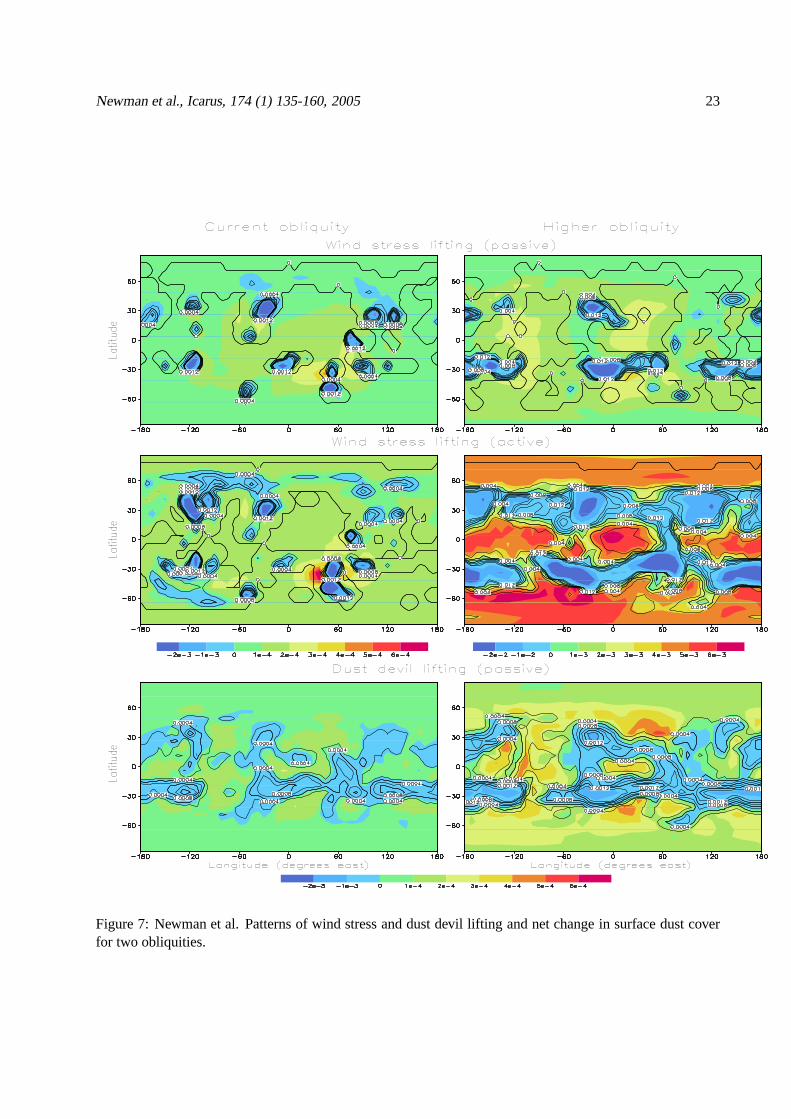
Figure 7 shows the thickness of dust lifted (contours) in oneyear and the net change in surface dust
thickness (shaded) after one year, using the wind stress (top row) and dust devil (bottom row) lifting param-
eterizations and passive dust transport, foro=25◦ (experiment presPAS, left column) and 45◦ (experiment
o45PAS, right column). (The middle row shows results using wind stress lifting with active dust transport,
experiments presAC and o35AC, discussed in section 4.2.) The amount of wind stress lifting is greatly in-
creased foro=45◦, hence contour intervals ten times larger are used to plot both lifting and net accumulation.
An important point is that both lifting rates and depositionrates are needed to determine the net change
in surface dust cover. The zero lifting contour does not always coincide with the border between net accu-
mulation and net removal (where blue meets green in these plots), indicating the importance of transport and
deposition as well as lifting alone. (The zero lifting contour does not appear on the annual mean dust devil
lifting plots, as during the course of a year there is some lifting everywhere using the current parameteriza-
tion.) Regions in which some dust lifting occurs are often regions of net dust accumulation overall, due to
deposition rates exceeding lifting (this occurs over almost all northern high latitudes, for example).
In all simulations the pattern of dust deposition is determined partly by local re-deposition, explaining
for example the peak in dust accumulation between two regions of strong wind stress lifting in the Chryse
WBC region foro=25◦. Also important is fallout of dust which has been carried andmixed within the
main atmospheric circulation. At the dustiest periods, around the solstices, atmospheric dust is largely
transported across low and midlatitudes within a cross-equatorial Hadley cell. As air columns are forced up
over topography the dust within them will concentrate near the surface, increasing deposition rates. Also, in
the lower atmosphere dust is transported most rapidly across the equator (from the descending to the rising
branch) within the WBC regions, whereas in the intervening regions – primarily the uplands of Tharsis,
spanning the equator, and south from Arabia into Noachis – wind velocities are far smaller. Dust thus
has more time to fall to lower levels (eventually to the surface) before again being carried aloft. These
arguments depend on a relatively uniform distribution of dust within the Hadley cell, however. Thus the
strongest correlation between topography and deposition is found when most dust is lifted near the rising
Hadley cell branch, allowing time for it to be well mixed before nearing the surface again, and the weakest
Newman et al., Icarus, 174 (1) 135-160, 2005 23
Figure 7: Newman et al. Patterns of wind stress and dust devillifting and net change in surface dust coverfor two obliquities.

Newman et al., Icarus, 174 (1) 135-160, 2005 24
correlation is found when strong lifting also occurs near the descending branch. So for example a stronger
correlation is produced for passive wind stress lifting (top row of Fig. 7) at 45◦ (right) than at the current
obliquity (left).
The main feature of the passive wind stress lifting results is the strong net removal within the WBCs
and, increasingly as obliquity (hence the strength of the mean meridional circulation, and the strength and
area of associated summer westerlies) increases, within a zonal collar in southern mid-latitudes. Two regions
of net accumulation increasingly dominate, one centred on 30◦E and the other on 120◦W, both extending
between∼40◦ north and south of the equator (excluding regions of strong erosion between∼20◦ and 35◦S).
The details of this result are, however, sensitive to the dust loading prescribed in the MGCM. If dust levels
are increased in northern winter, for example, this will produce a stronger meridional circulation, resulting
in more lifting within the WBC regions and possibly significant lifting in a band of northern mid-latitudes.
These affects are discussed further for active dust simulations (which do have higher dust loadings at this
time of year) in section 4.
For dust devils the change in surface dust cover foro=45◦ can be plotted using the same contour intervals
as foro=25◦, due to the smaller increase in lifting rates as obliquity isincreased than for wind stress (as
discussed in section 3.2.1). These results suggest that dust devil lifting is probably less important at high
obliquities, relative to wind stress lifting, than it is at present. However, the fact that dust devils have little or
no link to the varying circulation at different obliquities, but rather to the less radically changing distribution
of solar heating, suggests that at low obliquities (when wind stress lifting is greatly reduced) dust devils may
be the main source of atmospheric dust.
3.2.3 Comparisons with observed dust deposits
Thermal inertia should be high in regions with little dust and low in regions where a lot of dust is present
(e.g. Jakosky et al. 2000), so may be used to assess the current surface dust distribution. Maps of thermal
inertia derived from MGS TES spectra are shown in e.g. Mellonet al. (2000) and Ruff and Christensen
(2002). Ruff and Christensen (2002) also extract a ‘dust cover index’ based on using both lambert albedo
and thermal inertia, though this is more representative of the material lying on the surface than thermal inertia
(which probably indicates the proportion of dust within thefirst few centimeters of the surface), hence there
are some differences. Thermal inertia is thus more useful inidentifying longer term accumulation and hence
thicker dust deposits. Based on the most recent thermal inertia maps, there is a large region of high dust

Newman et al., Icarus, 174 (1) 135-160, 2005 25
content over Arabia (∼10◦W – 60◦E, 10◦S – 40◦N), and another broad region of high dust content stretching
from Elysium through Amazonis and over Tharsis (∼140◦– 180◦E and 180◦– 70◦W, covering most latitudes
from 15◦S – 40◦N).
If the observed regions of high dust content formed recently(say in the last 200,000 years, during which
time obliquity was close to its present value), and if local dust production (via erosion) is ignored, then
such regions should coincide with MGCM predictions of peak dust accumulation for the current obliquity.
If, however, the observed regions formed over much longer timescales, or were mostly formed at a time in
the past when higher obliquities dominated, they should be abetter match to predictions of peak accumu-
lation regions at higher obliquities, when many times more lifting probably occurs, resulting in far greater
accumulation rates.
Considering first wind stress dust lifting using passive dust transport (upper row of Fig. 7), peak ac-
cumulation occurs in the southern hemisphere for the current obliquity (left plot) and there is no apparent
anticorrelation between this plot and maps of thermal inertia. At higher obliquities – at 45◦ (right plot), and
also at 35◦ (not shown) – there are two other regions of peak accumulation further north, coinciding with the
Arabia and Tharsis regions observed to have high dust content. This suggests that the dust observed in these
areas may have accumulated over longer timescales, or have mostly taken place more than 500,000 years
ago (when Mars last had obliquities of∼35◦ or greater). Yet for all obliquities the MGCM fails to predict
peak accumulation over the Amazonis or Elysium regions observed to have high dust content.
The accumulation rates predicted by the MGCM can be used to provide an estimate of the age of these
deposits if their thickness is known. Christensen (1986) estimated the thickness of the low thermal inertia
regions to be between 0.1 and 2m, using thermal, radar and visual data. Obliquities have varied between
15◦ and 35◦ over the past 4Myrs, being roughly equally split between being greater than or less than 25◦.
A conservative estimate of the mean accumulation rate during this period is therefore that for 25◦ (given
that accumulation is greatly reduced for low obliquities, but is considerably more than doubled foro=35◦),
∼1.5×10⁻⁴cm yr−1 in central Arabia. This gives an upper limit on their age as between∼67,000 and 1.3
million years. There is an inconsistency here, noted also byHaberle et al. (2003), in that the results show
large parts of these regions to have been accumulating dust for all obliquities (presumably going back many
millions of years), but also imply that, if the estimated thicknesses are correct, they can only have begun
forming ∼1.3Myr in the past. This would suggest either that the net accumulation rates predicted using
wind stress lifting and passive dust transport are overestimates of the true values, or that the thicknesses

Newman et al., Icarus, 174 (1) 135-160, 2005 26
estimated by Christensen (1986) are much too small.
The above analysis did not consider the effects of dust devillifting. Looking at the pattern of dust
accumulation for dust devils, the net removal in e.g. central Arabia and over much of Tharsis would bring
down accumulation rates in these specific regions. Dust removal by dust devils would become less important
relative to the effects of wind stress lifting at higher obliquities, which might help to explain the closer
similarity between high obliquity accumulation patterns and currently observed surface dust content. But
wind stress lifting with active dust transport can also produce erosion over much of the high dust content
regions (see section 4.2). Clearly, to model dust accumulation rates correctly both wind stress lifting, dust
devil lifting and the effects of radiatively active dust transport should be included.
3.2.4 Net polar dust accummulation and the polar layered terrain
Figure 8 shows the change in thickness of polar dust depositsover one year for four obliquities (exper-
iments o15PAS, presPAS, o35PAS and o45PAS), using passive dust transport and wind stress lifting. Here
polar is defined as 75◦–90◦N and S. The absence of dips in these curves demonstrates the lack of any net
removal from polar regions. There are several clear trends –firstly, increased accumulation at both poles
as obliquity is increased, due largely to greater atmospheric dust levels overall. Secondly, as obliquity is
increased the pole gaining most dust switches from the northto the south. Lastly, as obliquity is increased
the relative accumulation during northern summer becomes increasingly important in these passive dust ex-
periments. Unfortunately, due to the complex nature of the results described here, the above trends will not
necessarily be valid for all dust scenarios, and when activedust is used only the first is certain to hold for all
parameter values.
Relative deposition rates over the north and south poles depend on atmospheric transport as much as
on where dust is lifted. Provided there is a moderately strong meridional circulation, polar deposition over
the winter pole is generally due more to upper level, cross-equatorial transport of dust lifted in the summer
hemisphere than to dust lifting at high winter latitudes. For o=25◦, for example, much of the dust deposited
over the north pole after Ls∼250◦ was lifted in the 22.5◦–45◦S range (see Fig. 6) then transported into the
winter hemisphere. Only some of this lifted dust reaches higher summer latitudes, to produce a smaller
increase in dust thickness over the south pole.
During northern winter foro=45◦, however, there is clearly transport over the summer (south) as well
as the winter (north) pole, with greater dust accumulation over the south pole despite the cross-equatorial

Newman et al., Icarus, 174 (1) 135-160, 2005 27
Obliquity=15 degrees
0 30 60 90 120 150 180 210 240 270 300 330 00.00
0.05
0.10
0.15
Chan
ge in
pola
r dus
t thic
knes
s (m
icron
s)
Obliquity=25 degrees
0 30 60 90 120 150 180 210 240 270 300 330 00.00
0.10
0.20
0.30
0.40
0.50
0.60
Chan
ge in
pola
r dus
t thic
knes
s (m
icron
s)
Obliquity=35 degrees
0 30 60 90 120 150 180 210 240 270 300 330 0Areocentric longitude Ls
0.0
0.2
0.4
0.6
0.8
1.0
1.2
1.4
Chan
ge in
pola
r dus
t thic
knes
s (m
icron
s)
Obliquity=45 degrees
0 30 60 90 120 150 180 210 240 270 300 330 0Areocentric longitude Ls
0
2
4
6
Chan
ge in
pola
r dus
t thic
knes
s (m
icron
s)
____ North pole (75-90 N)
_ _ _ South pole (75-90 S)
Figure 8: Newman et al. Polar dust accumulation for four obliquities using wind stress lifting.
circulation being stronger than during northern summer. This is due in part to the low level branch of the
Hadley cell extending further polewards for higher obliquities. It therefore carries more of the dust raised
in southern mid-latitudes further towards the pole, beforecarrying much of it to higher levels and into the
opposite hemisphere. For greater dust opacities a tidally forced cell, which rises in summer mid-latitudes
and descends over the summer pole, may also increase poleward dust transport.
Overall, the passive dust transport results suggest that dust deposition over south polar regions is minimal
for low obliquities, increasing to extremely large amountsfor high obliquities. Over north polar regions, dust
deposition is small (though greater than in the south) for low obliquities, increasing to very large amounts
(but less than in the south) for high obliquities. How this may impact the formation of of the polar layered
terrain would require careful modeling of water ice as well as dust deposition (including dust scavenging
during ice formation).
Dust devils (see Fig. 9) show a similar trend of peak accumulation over the north pole at low obliquities,
this switching gradually to the south pole as obliquity is increased. The main difference is that polar accu-
mulation rates are actually higher in the north foro=15◦ than foro=25◦ (and are comparable in the south).
Polar dust thickness also increases more gradually than forwind stress lifting, particularly at low obliquities.
These differences are due to the broader spread of locationsand times over which dust devil lifting occurs
(relative to wind stress lifting), meaning that dust devil lifting is more affected by increases in the area of

Newman et al., Icarus, 174 (1) 135-160, 2005 28
Obliquity=15 degrees
0 30 60 90 120 150 180 210 240 270 300 330 00
2
4
6
8
10
12
14
Chan
ge in
pola
r dus
t thic
knes
s (m
icron
s)
Obliquity=25 degrees
0 30 60 90 120 150 180 210 240 270 300 330 00
2
4
6
8
10
Chan
ge in
pola
r dus
t thic
knes
s (m
icron
s)
Obliquity=35 degrees
0 30 60 90 120 150 180 210 240 270 300 330 0Areocentric longitude Ls
-0
2
4
6
8
10
12
Chan
ge in
pola
r dus
t thic
knes
s (m
icron
s)
Obliquity=45 degrees
0 30 60 90 120 150 180 210 240 270 300 330 0Areocentric longitude Ls
0
5
10
15
20
Chan
ge in
pola
r dus
t thic
knes
s (m
icron
s)
____ North pole (75-90 N)
_ _ _ South pole (75-90 S)
Figure 9: Newman et al. Polar dust accumulation for four obliquities using dust devil lifting.
the winter hemisphere covered by CO2 ice (which prevents lifting). Ato=15◦ for example, dust devil lifting
can continue to∼55◦N throughout the year, whereas ato=25◦ no lifting occurs north of∼40◦N for almost
a third of the year. At higher obliquities, however, increased lifting rates during local summer more than
compensate for the loss of ice-free surface in the fall to spring hemisphere, hence accumulation rates at
o=35◦ are higher than those at 25◦. These results reinforce the idea that dust devil lifting may become more
important to the rearrangement of surface dust at low obliquities.
4 The effect of varying obliquity with radiatively active dust transport
4.1 The atmospheric circulation and dust lifting
The experiments shown previously used a single, prescribeddust distribution, which was not strictly
consistent with the circulation produced and the predicteddust lifting. The experiments described here, using
parameterized lifting and radiatively active dust transport, allow feedbacks to occur and the dust distribution
to evolve consistently, and should therefore better represent the true behavior on Mars. These experiments
(presAC and o35AC) include wind stress lifting only (ignoring here the effect of ‘background’ dust devil
lifting) with the same lifting parameters and threshold stresses used at both obliquities to produce results
which are consistent with each other, as for the passive runs.

Newman et al., Icarus, 174 (1) 135-160, 2005 29
u; Obliquity = 25 degrees
-90 -60 -30 0 30 60 900
20
40
60
Pseu
do-h
eigh
t abo
ve g
eoid
in k
m
-60
-20
20
20
20
60
60
u; Obliquity = 35 degrees
-90 -60 -30 0 30 60 900
20
40
60
-180
-120
-60
-600
00
60
T; Obliquity = 25 degrees
-90 -60 -30 0 30 60 90Latitude in degrees
0
20
40
60
Pseu
do-h
eigh
t abo
ve g
eoid
in k
m
150
15017
0170
170
190
190
190
210230
T; Obliquity = 35 degrees
-90 -60 -30 0 30 60 90Latitude in degrees
0
20
40
60
180
205
205
230
230
230
255
Figure 10: Newman et al. A zonal mean solsticial circulationfor o=25◦ and 35◦ with active dust.
Results are shown foro=25◦ and 35◦ only, because the positive feedbacks produced such high opaci-
ties aboveo=35◦ that the MGCM’s radiative transfer scheme became unstable.As discussed in section 6,
however, it is likely that such rapid growth in dust levels would not occur in reality.
The passive dust experiments for different obliquities already differed in terms of the strength of the sum-
mer meridional circulation and associated wind stress lifting. The first order effect of including radiatively
active dust transport is therefore to enhance these differences due to positive feedbacks between circulation
strength and dust lifting. Figure 10 shows an increase in thestrength of the northern winter circulation for
both obliquities (the passive dust results foro=35◦ were intermediate between those foro=25◦ ando=45◦
shown in Fig. 3) when active dust transport is used. The increase is far greater foro=35◦, however, with
different contour levels and arrow lengths even being required. And whereas for passive dust the southern
summer wind stress lifting peak in the 22.5◦– 45◦S latitude band was nine times larger for o=35◦(not shown)
than for o=25◦, Fig. 11 shows that it is more than thirty times larger for theactive dust case. Ato=35◦ the
strong positive feedbacks on lifting during southern summer produce such huge opacities at this time of
year that this peak completely dwarfs that during northern summer, which is however still larger than that
produced in the passive case.
Second order effects, which include interactions between the atmospheric dust distribution and atmo-

Newman et al., Icarus, 174 (1) 135-160, 2005 30
Obliquity=25 degrees
0 30 60 90 120 150 180 210 240 270 300 330 0Areocentric longitude Ls
0.000
0.002
0.004
0.006
0.008
Dust
lifting
rate
(cm
/year
)
Obliquity=35 degrees
0 30 60 90 120 150 180 210 240 270 300 330 0Areocentric longitude Ls
0.00
0.05
0.10
0.15
0.20
67.5-90 N
45-67.5 N
22.5-45 N
0-22.5 N
0-22.5 S
22.5-45 S
45-67.5 S
67.5-90 S
Figure 11: Newman et al. Wind stress dust lifting foro=25◦ and 35◦ with active dust.
spheric wave forcing, and the presence of local feedbacks (positive and negative) between dust distribution
and flow regimes, are more dependent on the exact details of the wind stress parameterization used. These
include, for example, the addition of several strong lifting peaks in the northern hemisphere during summer
for the activeo=25◦ case, resulting from strong positive feedbacks on lifting at the edge of localized dust
clouds in a relatively clear atmosphere.
A further effect is the smaller seasonal CO2 ice cap which forms in the northern hemisphere during
winter for o=35◦, compared to the passive dust result. This may be due to far greater adiabatic warming
being caused by stronger downwelling in northern high latitudes (though eddy heat fluxes probably play at
least a minor role). This allows dust lifting potentially toextend roughly 15◦ further to the north compared
with the passive simulation which, as discussed below, has strong implications for net surface dust removal.
It also affects the dominant wind direction in northern midlatitude regions, which returns to being from the
NE during winter (as predicted for the present day) rather than winds from the WSW during summer being
expected to dominate as obliquity is increased. Hence therecould be a significant impact on the conclusions
of section 3.1.3 if such high dust loadings and strong circulations actually occur at high obliquities (see
discussion in section 6.1).

Newman et al., Icarus, 174 (1) 135-160, 2005 31
4.2 Regions of dust accumulation
The middle row of Fig. 7 shows dust lifting and net accumulation for the active dust experiments pre-
sAC (left column) and o35AC (right column). At the surface the far stronger, broader Hadley circulations
produced in active dust runs as obliquity is increased produce stronger meridional flows across the equator
and extend the strong associated zonal winds to higher latitudes. This has the effect of increasing the amount
of net dust removal within the WBC flows, resulting in net erosion in a band stretching north across the
equator from Hellas for theo=35◦ simulation. There is also net erosion over nearly the entire20◦– 45◦S
latitude band during southern summer (where strong westerlies develop). Erosion also occurs in northern
mid-latitudes during northern summer, though it is less significant due to the weaker circulation at this time
of year.
There is increased dust removal from high latitudes in both hemispheres for the present day (o=25◦)
active dust simulation, due to changes in the amount and vertical distribution of dust compared to that which
was prescribed in the passive dust case. For example, lower opacities in northern spring result in stronger
cap edge flows and increased baroclinic wave activity, as expected (see respectively Siili et al. 1999; Zurek
et al. 1992), hence more associated dust lifting.
The more extensive circulations at both obliquities (particularly for o=35◦) lead to increased poleward
transport of dust. Ato=35◦, the combination of this with a far dustier atmosphere therefore produces greatly
increased polar accumulation rates (both relative too=25◦ active results and relative too=35◦ results using
passive dust transport).
For sufficiently high dust loadings there is substantial neterosion in northern mid-latitudes during south-
ern summer also (as shown in the high obliquity dust lifting plot of Fig. 11). Easterlies form here (via
conservation of angular momentum) as the strong return flow of the Hadley cell’s lower branch moves equa-
torward in the northern hemisphere, and produce particularly high near-surface wind stresses due to the
higher surface pressure over the lower topography in that hemisphere. These easterlies were present (though
weaker) in the passive dust simulation, but there was extensive CO2 ice cover (to∼30◦N at Ls=300◦). For
the active case, however, the surface is free of ice to∼45◦N by this time of year, allowing substantial dust
removal from the mid-latitude regions, as shown in the middle right plot of Fig. 7.

Newman et al., Icarus, 174 (1) 135-160, 2005 32
5 The effect of varying eccentricity and areocentric longitude of perihelion
5.1 The atmospheric circulation
Obliquity variations change the relative latitudinal distribution of solar insolation away from equinox,
and thus have a major effect on polar cap extent and on the peakforcing location of the meridional circula-
tion, both of which strongly affect near-surface winds. Varying Mars’s eccentricity or areocentric longitude
of perihelion, by contrast, changes the amount by which the response to solar heating at a particular time of
year dominates, and the time of year at which this occurs. In general, therefore, the effect on the general
circulation and wind stress dust lifting is less significantthan the effect due to obliquity variations, although
changes to the amount of seasonal ice cover at a given time of year can have a significant impact. The timing
of perihelion decreases in importance as eccentricity is decreased (ceasing to matter for a circular orbit).
But for moderate to high eccentricities, and with a constantvalue of obliquity, the atmospheric response is
determined by the extent to whichl aligns with a solstice or equinox (the former producing stronger circu-
lations than the latter). Ifl occurs near a solstice, the response will also depend on whether it is northern
winter or summer (the former again producing stronger circulations than the latter, due to the effects of the
hemispheric dichotomy discussed below).
Figure 12 shows zonally averaged temperatures and zonal winds, and the residual mean circulation, for
both solstices for a simulation withe=0, but otherwise with present day orbital settings (experiment e0PAS).
The distribution of solar insolation from summer to winter latitudes is therefore the same for both northern
and southern summer. For a featureless, smooth planet this would result in almost identical distributions
of solar heating (assuming constant or mirror image dust loadings) and mirror image solsticial circulations.
This is clearly not the case for Mars, the main feature of Fig.12 being the asymmetry between the solsticial
circulations, with that during northern winter significantly stronger.
Figure 13 shows the same results for simulations in which perihelion occurs in northern summer (l=71◦),
at exactly the opposite time of year to that at which perihelion presently occurs, but otherwise with present
day settings (experiment l71PAS). For a featureless, smooth planet the northern summer (winter) circula-
tion would therefore be expected to be a mirror image of that currently produced during northern winter
(summer). Again, this is not the case for Mars, with the circulation at northern winter solstice forl=71◦
approximately as strong as at northern summer solstice (if not stronger), despite coinciding with aphelion
(when roughly a third less solar insolation is received).

Newman et al., Icarus, 174 (1) 135-160, 2005 33
u; Ls=90 degrees
-90 -60 -30 0 30 60 900
20
40
60
Pseu
do-h
eigh
t abo
ve g
eoid
in k
m -60
-20
-20
20
20
u; Ls=270 degrees
-90 -60 -30 0 30 60 900
20
40
60
-60 -20
-20
20
20
60
T; Ls=90 degrees
-90 -60 -30 0 30 60 90Latitude in degrees
0
20
40
60
Pseu
do-h
eigh
t abo
ve g
eoid
in k
m
150
150
170
190
210
230
T; Ls=270 degrees
-90 -60 -30 0 30 60 90Latitude in degrees
0
20
40
60
150
150
170
170
190210
Figure 12: Newman et al. The zonal mean solsticial circulations fore=0.
u; Ls=90 degrees
-90 -60 -30 0 30 60 900
20
40
60
Pseu
do-h
eigh
t abo
ve g
eoid
in k
m -60
-20
-20
20
20
60
u; Ls=270 degrees
-90 -60 -30 0 30 60 900
20
40
60
-60 -20 20
20
60
T; Ls=90 degrees
-90 -60 -30 0 30 60 90Latitude in degrees
0
20
40
60
Pseu
do-h
eigh
t abo
ve g
eoid
in k
m
150170
170
190
210
230
T; Ls=270 degrees
-90 -60 -30 0 30 60 90Latitude in degrees
0
20
40
60
150
150
150
170
190
210
Figure 13: Newman et al. The zonal mean solsticial circulations forl=71◦.

Newman et al., Icarus, 174 (1) 135-160, 2005 34
The reason for these asymmetric results is that Mars is neither featureless nor smooth, its surface having
significant variations of albedo and thermal inertia (affecting the absorption of radiation) and topography
(affecting the height above the geoid to which radiation penetrates and at which near-surface air is heated
by the ground, and also impeding the flow). These can also act in more subtle ways by changing the wave
structure of the atmospheric flow. Joshi et al. (1995) pointed out that the observed asymmetry in Mars’s
solsticial circulations is not simply due to perihelion occurring during southern summer, and Richardson and
Wilson (2002) showed the presence of an annual mean bias by considering the effect of changing perihelion
on the simulated annual mean mass streamfunction. They found this to be dominated by the northern winter
hemisphere cell for bothl=71◦ and 251◦, whereas the southern winter hemisphere cell would have dominated
for l=71◦ if the orbital configuration (and magnitude of solar insolation) were most important. They then
showed that this bias was essentially eliminated if the hemispheric dichotomy in topography was removed.
Takahashi et al. (2003) have explored this further, and shown a similar dependence on the elevated southern
hemisphere using another Mars general circulation model.
Such biases can be most easily investigated fore=0, since for a featureless and smooth planet this sit-
uation would produce mirror image circulations at the two solstices as well as a highly symmetric mass
streamfunction when averaged over the entire year. Figure 14 shows annual mean mass streamfunctions for
e=0 under different conditions: (1) no alterations; (2) topographic dichotomy removed; (3) uniform, smooth
surface but with MGS Mars Orbiter Laser Altimeter (MOLA) topography used to model surface and gravity
wave drag; and finally, (4) a uniform, smooth surface withoutdrag. The plot for case (4) is, as expected,
completely symmetric, since there are no longer any hemispheric asymmetries, yet the case (2) plot is sig-
nificantly more symmetric than that for case (1), indicatingthe importance of the hemispheric topographic
dichotomy in biasing the mass streamfunction.
If the solsticial circulations are examined for the different cases, removing the dichotomy has a similar
effect in reducing the bias in regions where the mass streamfunction has significant amplitude. Figure 15
shows zonal mean temperatures and the residual mean circulation for cases (2) and (4). Comparing these
results with those for case (1), shown in Fig. 12, the circulation is far more symmetric between the solstices
below∼40km and away from high latitudes once the topographic dichotomy has been removed. Above this
and at higher latitudes, however, the circulation is still stronger in northern than in southern winter, with a far
greater polar warming over the winter pole. Not until all asymmetries have been removed is the circulation
(including near-surface wind patterns) completely symmetric.

Newman et al., Icarus, 174 (1) 135-160, 2005 35
Case 1
-90 -60 -30 0 30 60 900
10
20
30
40
Pseu
do-h
eigh
t abo
ve g
eoid
in k
m
-5
-5
-1 3 7
Case 2
-90 -60 -30 0 30 60 900
10
20
30
40
-5
-1 -1
3
7
Case 3
-90 -60 -30 0 30 60 90Latitude
0
10
20
30
40
Pseu
do-h
eigh
t abo
ve g
eoid
in k
m
-5
-13 3
7
Case 4
-90 -60 -30 0 30 60 90Latitude
0
10
20
30
40
-5
-1
-1
-1
3
37
Figure 14: Newman et al. Annual mean mass streamfunctions for four e=0 cases.
Case 2; Ls=90 degrees
-90 -60 -30 0 30 60 900
20
40
60
Pseu
do-h
eigh
t abo
ve g
eoid
in k
m
150
150
170
190
210
230
Case 2; Ls=270 degrees
-90 -60 -30 0 30 60 900
20
40
60
150
15017
0
170
190210230
Case 4; Ls=90 degrees
-90 -60 -30 0 30 60 90Latitude in degrees
0
20
40
60
Pseu
do-h
eigh
t abo
ve g
eoid
in k
m
150
150
150
150
170
170
190
210
230
Case 4; Ls=270 degrees
-90 -60 -30 0 30 60 90Latitude in degrees
0
20
40
60
150
150
150
170
170
190
210230
Figure 15: Newman et al. Zonal mean temperatures and residual mean circulations at solstice for twoe=0simulations.

Newman et al., Icarus, 174 (1) 135-160, 2005 36
Eccentricity=0
0 30 60 90 120 150 180 210 240 270 300 330 00.0000
0.0002
0.0004
0.0006
0.0008
Dus
t lift
ing
rate
(cm
/yea
r)
Perihelion at Ls=71 degrees
0 30 60 90 120 150 180 210 240 270 300 330 00.0000
0.0005
0.0010
0.0015
0.0020
0.0025
0.0030
Perihelion at Ls=180 degrees
0 30 60 90 120 150 180 210 240 270 300 330 0Areocentric longitude Ls
0.0000
0.0005
0.0010
0.0015
0.0020
Dus
t lift
ing
rate
(cm
/yea
r)
Current orbital settings
0 30 60 90 120 150 180 210 240 270 300 330 0Areocentric longitude Ls
0.0000
0.0005
0.0010
0.0015
0.0020
0.0025
67.5-90 N45-67.5 N22.5-45 N0-22.5 N
0-22.5 S22.5-45 S45-67.5 S67.5-90 S
Figure 16: Newman et al. Wind stress dust lifting for two eccentricities and two longitudes of perihelion.
5.2 Dust transport
Figure 16 shows the pattern of wind stress dust lifting in different latitude bands for thee=0, l=71◦ and
l=180◦ passive dust transport simulations, with results for current orbital settings shown again for compar-
ison. The pattern of dust lifting fore=0, with far more lifting after Ls∼180◦ than earlier in the year, is
(apart from having more lifting peaks during northern summer) very similar to that for the present day. This
demonstrates clearly that asymmetry between southern and northern summer solstice still exists in the ab-
sence of a time of peak solar insolation. Results forl=180◦ are similar, with northern winter again dominant
in terms of lifting. By contrast, the results forl=71◦ do show a significant switch from southern to northern
summer dominance, far more so than might have been anticipated by the change in circulation strength. This
is almost entirely due to the larger seasonal north polar caponly having receded to∼60◦N by late spring
(Ls∼50◦), resulting in strong off-cap flows and large amounts of lifting at its edge.
Figure 17 shows the change in polar dust thickness with time for one year of thee=0, l=71◦ andl=180◦
simulations, again with results also shown for the current settings. Forl=71◦ the north pole receives more
dust than the south during northern summer. The circulationis weak compared to the southern summer
circulation forl=251◦, thus this is due to a combination of reduced cross-equatorial transport by the Hadley

Newman et al., Icarus, 174 (1) 135-160, 2005 37
Eccentricity=0
0 30 60 90 120 150 180 210 240 270 300 330 00.00
0.05
0.10
0.15
0.20
Chan
ge in
pola
r dus
t thic
knes
s (m
icron
s)
Perihelion at Ls=71 degrees
0 30 60 90 120 150 180 210 240 270 300 330 00.0
0.1
0.2
0.3
Chan
ge in
pola
r dus
t thic
knes
s (m
icron
s)
Perihelion at Ls=180 degrees
0 30 60 90 120 150 180 210 240 270 300 330 0Areocentric longitude Ls
0.00
0.10
0.20
0.30
0.40
0.50
Chan
ge in
pola
r dus
t thic
knes
s (m
icron
s)
Current orbital settings
0 30 60 90 120 150 180 210 240 270 300 330 0Areocentric longitude Ls
0.00
0.10
0.20
0.30
0.40
0.50
0.60
Chan
ge in
pola
r dus
t thic
knes
s (m
icron
s)
____ North pole (75-90 N)
_ _ _ South pole (75-90 S)
Figure 17: Newman et al. Polar dust accumulation for two eccentricities and two longitudes of perihelion.
cell’s upper branch and increased dust lifting at fairly high northern latitudes.
In all cases the amount accumulated at both poles at any time tends to be increased close to perihelion
and decreased close to aphelion, though in the absence of these (e=0) there is greater accumulation during
northern winter, with results for the other cases showing a northern winter bias also. Overall, accumulation
rates are higher as perihelion nears northern winter solstice (since overall this produces the strongest circu-
lations and lifting rates), and are lowest when solar insolation is spread evenly through the year (fore=0).
There is also more accumulation over the north pole than the south for the three cases shown (suggesting
that north polar accumulation probably dominates for all orbital configurations havingo ≤25◦).
6 Conclusions
6.1 Changes to the atmospheric circulation due to changing orbital parameters
The MGCM predicts that as Mars’s orbital parameters vary with time, the greatest changes to atmo-
spheric circulation and dust transport are due to variations in obliquity. Increasing obliquity affects the
relative latitudinal distribution of solar insolation (away from equinox), which has a major effect on polar
cap extent and on the peak forcing location of the meridionalcirculation near solstice. The seasonal CO2 cap
extends over more of the winter hemisphere, and the peak in time-averaged solar forcing occurs at higher

Newman et al., Icarus, 174 (1) 135-160, 2005 38
latitudes producing broader and stronger meridional (Hadley) circulations.
At low obliquities permanent CO2 ice caps form at both poles, significantly reducing mean surface
pressures (to∼40Pa foro=5◦, and∼350Pa foro=15◦), hence also lowering near-surface densities and thus
wind stresses.
When active dust transport is included, a wind stress lifting parameter selected to produce realistic results
for the current obliquity produces huge amounts of lifting for eveno=35◦, due to the strong positive feed-
backs between atmospheric dust loading, the atmospheric circulation and wind stress lifting. Simulations for
o=45◦ rapidly become unstable (see comments below). In addition,the stronger circulations produced in a
dustier atmosphere lead to increased downwelling and adiabatic warming at winter high latitudes, resulting
in smaller seasonal caps than in passive runs which in turn affects the surface wind distribution and dust
lifting.
The primary effect of varying eccentricity is to change the impact of varying the areocentric longitude
of perihelion, which determines when the solar forcing is strongest. The atmospheric circulation is strongest
whenl aligns with solstice, and there is also a bias from the Martian topography, resulting in the strongest
circulations for highe whenl is in northern winter.
Near-surface winds associated with a solsticial Hadley circulation (e.g. cross equatorial WBCs and
summer midlatitude westerlies) increase in strength as this circulation intensifies at higher obliquities, in-
creasingly dominating over baroclinic, thermal contrast (e.g. cap edge) and topographic flows. Along with
changes in the position of the cap edge, these effects produce significant changes in surface wind directions
as well as magnitudes.
For passive dust transport the MGCM predicts that at higher obliquities the dominant northern midlati-
tude (∼25◦– 50◦N) winds should be from the SW during summer (rather than fromthe NE during winter, as
at present). This is due to the presence of a stronger, broader Hadley cell (and its associated surface winds)
during summer, and increased ice cover (reducing near-surface temperature gradients, hence lowering wind
magnitudes, far from the cap edge) during winter, as obliquity is increased. If active dust transport is in-
cluded, however, the MGCM predicts a smaller seasonal ice cap than in the passive run, hence the dominant
winds are once again from the NE during winter, implying thatcare is required in interpreting such results.
Newman et al., Icarus, 174 (1) 135-160, 2005 39
6.2 Changes to dust lifting and deposition due to changing orbital parameters
As obliquity increases, for wind stress lifting, the stronger westerlies produced in summer midlatitudes
increase dust lifting within bands centred on∼30◦ latitude (though these move slightly poleward with obliq-
uity, particularly foro=45◦). Lifting peaks at the poleward edge of WBC regions, with smaller peaks in
equatorial regions within the WBC flows.
There is a smaller change in both the magnitude and pattern ofdust devil lifting as obliquity increases.
Lifting peaks at∼25◦ latitude in local summer for all obliquities, the latitude at which atmospheric temper-
atures lag surface temperatures most strongly in all cases.Peak lifting rates increase more gradually with
obliquity than for wind stress lifting, being less tied to the rapidly increasing meridional circulation.
For active dust transport, ato=35◦ lifting occurs across broader midlatitude regions due to the strong
winds associated with stronger, broader meridional circulations in the dustier atmosphere produced. Lifting
from northern midlatitudes in winter is enhanced if a smaller seasonal cap forms, though the latter depends
on how realistic the high obliquity active dust simulationsare in terms of the peak opacities and circulations
produced. Care must be taken in interpreting these results as a true representation of what would occur at
higher obliquities, and the changes in circulation strength and extent of dust removal shown in Figs. 10 and
11 respectively should be taken as an extreme limit on what might actually occur.
In all cases, the pattern of dust deposition is determined partly by local re-deposition and partly by
the fallout of dust which has been carried and mixed within the main atmospheric circulation. There is
slight preferential deposition over high topography within the Hadley cell’s extent. The effect is strongest
when lifting peaks near the rising Hadley cell branch, as this results in the dust distribution being relatively
uniform by the time it nears the surface again. Dust lifted near the descending branch, however, will tend to
be redeposited before entering the main circulation, and atlongitudes similar to those where lifting occurred
(which generally peak in the WBC regions which are between topographic highs), thus compensating for
the former effect.
6.3 Changes to dust accumulation due to changing orbital parameters
The inclusion of a dust transport scheme within the MGCM is necessary to enable radiatively active
dust transport experiments, of key importance in representing real Mars, given the strong feedbacks on dust
lifting. But it is also crucial for this study because it allows the MGCM to a) predict dust deposition and
net accumulation, as well as dust lifting, and b) constrain lifting parameters by comparing the simulated

Newman et al., Icarus, 174 (1) 135-160, 2005 40
atmospheric dust distribution with that observed. Together, (a) and (b) then allow quantitative comparisons
to be made between predicted and observed surface dust deposits.
Results show that the boundary between net erosion and net accumulation does not necessarily coin-
cide exactly with the zero lifting contour, and more importantly, that the amount of accumulation varies
considerably even within regions where only deposition occurs.
6.3.1 Potential long term dust deposits
As obliquity increases, regions of peak net dust accumulation north of∼30◦S are increasingly restricted
to Arabia and Tharsis, in agreement with observations of peak dust content here, though Amazonis and
regions around Elysium are less apparent in simulations than in observations.
For active dust transport, the scouring of dust from northern as well as southern midlatitudes at higher
obliquities limits the areas with peak accumulation to±15◦ of the equator, though the longitudinal match
to observations is improved. There is significant accumulation in Arabia and from Elysium, over Amazonis
through to Tharsis, with net erosion clearly peaking withinthe WBCs. Erosion over the Tharsis peaks is
reduced because of smaller slope winds in the dustier atmosphere. Accumulation south of the strong southern
hemisphere erosional band is due to enhanced polewards transport of dust raised in the south during summer.
The MGCM predicts current accumulation rates of∼1.5×10⁻⁴ cm/year in the Arabia region. The esti-
mated thickness of dust deposits here (Christensen 1986) then suggests that they were formed in∼67,000–
1.3 million years, though this timescale is inconsistent with the results shown here, since the MGCM predicts
that a large part of this region will accumulate dust over a range of orbital conditions. The greater correla-
tion between higher obliquity results and observations of dust content might suggest that they formed mostly
under higher obliquity conditions, but in this case the accumulation rates would have been even higher.
A small amount of lifting from these regions would result in lower net accumulation rates. Unfortunately,
lifting predicted here in both dust devil and active wind stress experiments does not produce this result,
instead scouring the northern half of dust and (in the case ofactive lifting) increasing net accumulation in
the equatorial areas and to the south. It is possible that theestimated dust thicknesses are too small, or that
a more complex model is required, with combined wind stress and dust devil lifting, and active transport.
A full representation would also include a limited surface dust supply and ice scavenging, both of which
may limit the strength of the storms and hence circulations produced, strongly affecting lifting in northern
midlatitudes.

Newman et al., Icarus, 174 (1) 135-160, 2005 41
In summary, for high obliquities with wind stress lifting only, the MGCM predicts peak net dust accu-
mulation over the Tharsis and Arabia low thermal inertia regions. For stronger circulations (produced in an
active dust simulation) the MGCM predicts peak accumulation over the equatorial portions of these regions
and also in the low thermal inertia regions of Elysium and Amazonis. If there is no surface ice cover in
northern mid-latitudes in winter for the latter case, or if dust devil lifting is included, there is net removal
from the more northerly portions of the low thermal inertia regions. This suggests that only the equatorial
low thermal inertia regions are dust sinks for all orbital settings, and thus that they may have the highest dust
content.
6.3.2 Polar accumulation rates
Dust devil and wind stress lifting is negligible over polar regions (defined as 75◦– 90◦) for all orbital
configurations shown, thus net accumulation here is solely due to deposition. As obliquity increases, polar
accumulation rates increase for wind stress lifting due to the higher dust loadings overall, and the stronger,
broader transport circulations (particularly for active dust) which carry more dust to the poles. The largest
accumulation rates occur when perihelion coincides with southern summer, and peak for high values of ec-
centricity (giving the strongest solar forcing at perihelion), with weaker rates as perihelion nears an equinox.
For dust devil lifting, polar accumulation rates also increase with obliquity aboveo=25◦, though less
rapidly as lifting (hence the dust load produced) is only slightly linked to the stronger surface winds. In active
dust simulations the negative feedbacks on dust devil lifting would further reduce this. Polar accumulation
rates are higher ato=15◦ than ato=25◦, due to the reduction in surface ice cover at the lower obliquity, which
is significant for dust devil lifting as it is more widespreadboth spatially and temporally. Thus polar dust
accumulation at low obliquities may be increasingly due to dust lifted by dust devils.
For all cases discussed, the pole receiving most dust shiftsfrom north to south as obliquity is increased.
For low obliquities much of the dust raised in the summer hemisphere is transported across the equator
without nearing the summer pole, hence peak lifting in southern summer midlatitudes produces more accu-
mulation at the north pole. At high obliquities, however, the meridional circulation extends closer to the pole
in both hemispheres, hence more of the dust raised in the south in summer reaches high southern latitudes
before being carried north, raising south polar accumulation rates.

Newman et al., Icarus, 174 (1) 135-160, 2005 42
6.4 Future work
The strength of positive feedbacks on wind stress dust lifting, particularly in high obliquity simulations,
is a major concern which must be addressed before work can progress. One effect absent from the MGCM
which would affect this is the process of dust scavenging by ice particles during nucleation. This will become
increasingly important at higher obliquities, when warmerpoles result in greatly increased atmospheric
humidity and cloud water ice (e.g. Jakosky et al. 1995; Mischna et al. 2003). A further effect of increased
water vapor abundances is the effect on surface water ice (rather than CO2 ice) cover, which may have a huge
impact if it prevents dust lifting in for example the northern mid-latitude regions activated during a global
dust storm. Mischna et al. (2003) predict water ice cover over most of the northern hemisphere in winter for
obliquities 35◦ and higher. Thus even if temperatures were raised sufficiently to prevent such a large CO2
ice cap forming, they would also need to be high enough, giventhe high partial pressures of water vapor
at this time, to prevent a large water ice cap forming, which could itself prevent the northern dust lifting.
Scavenging is also of major importance in predicting polar dust and ice accumulation rates for comparison
with observations of the polar layered terrain, and would require the inclusion of a water transport scheme
(currently being validated within the MGCM, Bottger et al.2004) as well as a microphysics scheme to
couple the two properly. Another effect not examined here isthe use of a finite dust supply on the Martian
surface, such that some regions can be entirely depleted of dust during a simulation. In preliminary MGCM
experiments this has been found to increase the amount of interannual variability, by continuously resetting
the surface boundary condition for dust lifting. These effects must be explored, and their impact assessed,
before the results such as those shown in section 4 can be judged to be realistic.
Acknowledgments.
We gratefully acknowledge support for this work from the UK Particle Physics and Astronomy Research
Council, and thank our reviewers for their suggestions and constructive criticism.
References.
Andrews, D. G., Holton, J. R., Leovy, C. B., 1987. Middle Atmosphere Dynamics, Academic Press, Orlando,
Florida.
Basu, S., Richardson, M. I., Wilson, R. J., 2004. Simulationof the Martian dust cycle with the GFDL Mars
GCM. J. Geophys. Res. (submitted).
Bottger, H. M., Lewis, S. R., Read, P. L., Forget, F., 2004. The effect of a global dust storm on simulations

Newman et al., Icarus, 174 (1) 135-160, 2005 43
of the Martian water cycle. Geophys. Res. Lett. (submitted).
Bridges, N. T., Greeley, R., Haldemann, A. F. C., Herkenhoff, K. E., Kraft, M., Parker, T. J., 1999. Ventifacts
at the Pathfinder landing site. J. Geophys. Res. 104, 8,595–8,615.
Cantor, B., James, P. B., Caplinger, M., Wolff, M. J., 2001. Martian dust storms: 1999 Mars Orbiter Camera
observations. J. Geophys. Res. 106, 23653–23687.
Christensen, P. R., 1986. Regional dust deposits on Mars: physical properties, age, and history. J. Geo-
phys. Res. 91, 3,533–3,545.
Clancy, R. T., Sandor, B. J., Wolff, M. J., Christensen, P. R., Smith, M. D., Pearl, J. C., Conrath, B. J.,
Wilson, R. J., 2000. An intercomparison of ground-based millimeter, MGS TES, and Viking atmo-
spheric temperature measurements: Seasonal and interannual variability of temperatures and dust
loading in the global Mars atmosphere. J. Geophys. Res. 105,9553–9571.
Edgett, K. S., Malin, M. C., 2000. Martian dust raising and surface albedo controls: Thin, dark (and some-
times bright) streaks and dust devils in MGS MOC high resolution images. Conference paper Lunar
and Planetary Science, XXXI.
Fanale, F. P., Salvail, J. R., 1994. Quasi-periodic atmosphere-regolith-cap CO2 redistribution in the Martian
past. Icarus 111, 305–316.
Fanale, F. P., Salvail, J. R., Banerdt, W. B., Saunders, R. S., 1982. Mars – The regolith-atmosphere-cap
system and climate change. Icarus 50, 381–407.
Fenton, L. K., Richardson, M. I., 2001. Martian surface winds: Insensitivity to orbital changes and implica-
tions for aeolian processes. J. Geophys. Res. 106, 32,885–32,902.
Ferri, F., Smith, P. H., Lemmon, M., Renno, N. O., 2003. Dustdevils as observed by Mars Pathfinder.
J. Geophys. Res. 108 (E12), doi:10.1029/2000JE001421.
Forget, F., Hourdin, F., Fournier, F., Hourdin, C., Talagrand, O., Collins, M., Lewis, S. R., Read, P. L.,
Huot, J.-P., 1999. Improved general circulation models of the Martian atmosphere from the surface
to above 80 km. J. Geophys. Res. 104, 24,155–24,175.
Greeley, R., Kraft, M. D., Sullivan, R., Wilson, G., Bridges, N., Herkenhoff, K., Kuzmin, R. O., Malin, M.,
Ward, W., 1999. Aeolian features and processes at the Mars Pathfinder landing site. J. Geophys. Res.
104, 8,573–8,584.
Greeley, R., Kraft, M. D., Kuzmin, R. O., Bridges, N. T., 2000. Mars Pathfinder landing site: Evidence for
a change in wind regime from lander and orbiter data. J. Geophys. Res. 105, 1,829–1,840.

Newman et al., Icarus, 174 (1) 135-160, 2005 44
Greeley, R., Bridges, N. T., Kuzmin, R. O., Laity, J. E., 2002. Terrestrial analogs to wind-related features at
the Viking and Pathfinder landing sites on Mars. J. Geophys. Res. 107, art. no. 5005.
Haberle, R. M., Leovy, C., Pollack, J. B., 1982. Some effectsof global dust storms on the atmospheric
circulation of Mars. Icarus 50, 322–367.
Haberle, R. M., Murphy, J. R. Schaeffer, J., 2003. Orbital change experiments with a Mars general circula-
tion model. Icarus 161, 66–89.
Jakosky, B. M., Henderson, B. G., Mellon, M. T., 1995. Chaotic obliquity and the nature of the Martian
climate. J. Geophys. Res. 100 E1, 1579–1584.
Jakosky, B. M., Mellon, M. T., Kieffer, H. H., Christensen, P. R., Varnes, E. S., Lee, S. W., 2000. The
thermal inertia of Mars from the Mars Global Surveyor Thermal Emission Spectrometer. J. Geo-
phys. Res. 105 E4, 9,643–9,652.
Joshi, M. M., Lewis, S. R., Read, P. L., Catling, D. C., 1995. Western boundary currents in the Martian
atmosphere: Numerical simulations and observational evidence. J. Geophys. Res. 100, 5,485–5,500.
Laskar J., Levrard, B., Mustard, J. F., 2002. Orbital forcing of the martian polar layered deposit. Nature 419,
375–377.
Lewis, S. R., Collins, M., Read, P. L., Forget, F., Hourdin, F., Fournier, F., Hourdin, C., Talagrand, O., Huot,
J.-P., 1999. A climate database for Mars. J. Geophys. Res. 104, 24,177–24,194.
Liu, J. J., Richardson, M. I., Wilson, R. J., 2003. An assessment of the global, seasonal, and interan-
nual spacecraft record of Martian climate in the thermal infrared. J. Geophys. Res. 108 (E8),
doi:10.1029/2002JE001921.
Mellon, M. T., Jakosky, B. M., Kieffer, H. H., Christensen, P. R., 2000. High-resolution thermal inertia
mapping from the Mars Global Surveyor Thermal Emission Spectrometer. Icarus 148, 437–455.
Mischna, M. A., Richardson, M. I., Wilson, R. J., McCleese, D. J., 2003. On the orbital forcing of Martian
water and CO2 cycles: A general circulation model study with simplified volatile schemes. J. Geo-
phys. Res. 108 (E6), doi:10.1029/2003JE002051.
Murphy, J. R., Pollack, J. B., Haberle, R. M. Leovy, C. B., Toon, O. B. Schaeffer, J., 1995. 3-dimensional
numerical simulation of Martian global dust storms. J. Geophys. Res. 100 (E12), 26,357–26,376.
Newman, C. E., Lewis, S. R., Read, P. L., Forget, F., 2002a. Modeling the dust cycle in a Mars gen-
eral circulation model. 1: Representations of dust transport processes. J. Geophys. Res. 107
(E12), doi:10.1029/2002JE001910.

Newman et al., Icarus, 174 (1) 135-160, 2005 45
Newman, C. E., Lewis, S. R., Read, P. L., Forget, F., 2002b. Modeling the dust cycle in a Mars general
circulation model. 2: Multi-annual radiatively active dust transport simulations. J. Geophys. Res.
107 (E12), doi:10.1029/2002JE001920.
Pollack, J. B., Toon, O. B., 1982. Quasi-periodic climate changes on Mars – a review. Icarus 50, 259–287.
Renno, N. O., Burkett, M. L., Larkin, M. P., 1998. A simple thermodynamical theory for Dust Devils.
J. Atmos. Sci. 55, 3,244–3,252.
Richardson, M. I., Wilson, R. J., 2002. A topographically forced asymmetry in the Martian circulation and
climate. Nature. 416,298–300.
Ruff, S. W., Christensen, P. R., 2002. Bright and dark regions on Mars: Particle size and mineralogi-
cal characteristics based on Thermal Emission Spectrometer data. J. Geophys. Res. 107 (E12),
doi:10.1029/2001JE001580.
Siili, T., Haberle, R. M., Murphy, J. R., Savijarvi, H., 1999. Modelling of the combined late-winter ice cap
edge and slope winds in Mars’ Hellas and Argyre regions. Plan. Space Sci. 47, 951–970.
Smith, M. D., 2004. Interannual variability in TES atmospheric observations of Mars during 1999–2003.
Icarus 167, 148–165.
Smith, M. D., Pearl, J. C., Conrath, B. J., Christensen, P. R., 2001. Thermal Emission Spectrometer results:
Atmospheric thermal structure and aerosol distribution. J. Geophys. Res. 106 (E10), 23,929-23,946.
Takahashi, Y. O., Fujiwara, H., Fukunishi, H., Odaka, M., Hayashi, Y. Y., Watanabe, S., 2003. Topograph-
ically induced north-south asymmetry of the meridional circulation in the Martian atmosphere.
J. Geophys. Res. 108 (E3), doi:10.1029/2001JE001638.
Toon, O. B., Pollack, J. B., Ward, W., Burns, J. A., Bilski, K., 1980. The astronomical theory of climatic
change on Mars. Icarus 44, 552–607.
Touma, J., Wisdom, J., 1993. The chaotic obliquity of Mars. Science 259, 1,294–1,297.
Ward, W. R., 1992. Long-term orbital and spin dynamics of Mars. In: Kieffer, H. H., Jakosky, B. M.,
Snyder, C. W., Matthews, M. S. (Eds.). Mars, The University of Arizona Press, Tucson, chap. 9,
pp. 298–320.
Zurek, R. W., Barnes, J. R., Haberle, R. M., Pollack, J. B., Tillman, J. E., Leovy, C. B., 1992. Dynamics of
the atmosphere of Mars. In: Kieffer, H. H., Jakosky, B. M., Snyder, C. W., Matthews, M. S. (Eds.).
Mars, The University of Arizona Press, Tucson, chap. 26, pp.835–933.