¢

MINISTRY OF SUPPLY

R. & M. No. 3039 (18,414)

A.R.C. Technical Report

A E R O N A U T I C A L R E S E A R C H C O U N C I L

R E P O R T S A N D M E M O R A N D A

The Theoretical Determination of Normal Modes and Frequencies

of Vibration

I. T . MINHINNICK

Crown CopyrigAt Reserved

LONDON • H E R MAJESTY'S STATIONERY OFFICE

I957

NINE SHILLINGS NET

The Theoretical Determination of Normal Modes and Frequencies of Vibration

By I. T . MINHINNICK

COMMUNICATED BY THE DIRECTOR-GENERAL OF SCIENTIFIC RESEARCH (AIR) , MINIST~Y OF SUFPI~'Z

Reports and Memoranda No. 3o39" January, z 956

Summary.--In this paper the various methods that have been devised for the determination of the natural frequencies and normal modes of aircraft are discussed and their accuracy and the amount of work that they entail are compared. An extensive bibliography is given. The discussion is mainly from the point of view of the flutter analyst, who commonly bases his analyses on the normal modes, but the description and comparison of the various methods should be of general interest.

1. Introduction.--By normal modes are mean t the natural modes of vibrat ion of the structure. They mus t strictly be defined for an idealized structure, one wi thout any structural damping vibrat ing in still air, the air being assumed to have only an inert ia effect. Such a system can vibrate freely wi th constant ampli tude at certain particular f requencies- - the natural frequencies. The mode of deformat ion of the sys tem at any one of these frequencies is t e rmed a normal mode because these modes are orthogonal with respect to bo th the mass distr ibution and the stiffness distr ibution o f the structure. For a real structure, which possesses structural damping, some energy must b e supplied to it for it to vibrate at constant ampli tude. This is wha t is done in a resonance test, in which a periodic excit ing force is applied over a range of frequencies. Maximum ampli tudes of vibrat ion will then occur at certain frequencies. If the s tructural damping is not very large, the frequencies at which these peak ampli tudes occur will be equal to the natural frequencies of the damping-free structure, and the modes of vibrat ion at these frequencies will be little different from the normal modes.

The calculation of normal modes, which will normal ly be done in the design stage of the aircraft, is impor tan t for several reasons, First, by examining the normal modes obta ined and part icularly the positions of the modal lines, it ma y be possible to tell whether flutter is likely or not, and in any case such an examinat ion will indicate what types of flutter should be investigated. It m ay also be possible to predict whether there is any likelihood of resonant vibration, due to the proximi ty of the natural frequencies to the forcing frequencies of the power plant. However, such frequencies are usually high overtone frequencies which are difficult to calculate accurately.

Further , the normal modes are commonly used for the actual flutter calculations. Theoretically, any set of independent deformat ion modes can be used as degrees of freedom in set t ing up the flutter equations, but from practical considerations we want to select those modes which give an accurate flutter speed when the number of chosen modes is small. This is more likely to be tile case when the modes 'are related to the actual structure, as the normal modes are, t han when the modes chosen are qui te arbitrary. I t has not, however, been conclusively demons t ra ted tha t t he normal modes are the best for this purpose. I t is possible wi th less effort to obtain other

* R.A.E. Report Structures 197, received 2nd May, 1956. (689~)

modes whioh are in some degree related to the particular structure, but an additional reason why it is desirable to use normal modes is because they can later be compared with the resonance-test mo des.

This paper is concerned with the theoretical calculation of normal modes. It reviews the various methods that have been devised and compares them for accuracy and the amount of work they entail. The methods fall into types, according to the type of equation used and the type of semi-rigidity assumed, and this fundamental classification is presented in section 2. The methods themselves are described and discussed in sections 3 to 10, in terms, for convenience, of either purely flexural or purely torsional vibrations of a beam. In sections 11 to 13 the discussion extends to the further complications that occur in practice: coupled flexure-torsion vibrations, the calculation of modes of complex structures, and the calculation of modes of a complete aircraft. A bibliography is given.

2. Types of Methods.--Before we can consider the calculation of the normal modes of a complete aircraft we must first consider the calculation of its component parts (wing, fuselage and tail unit) in isolation. The various methods by which these are calculated are based on one of three types of fundamental equation : the basic differential equation, the integral equation incorporating flexibility coefficients, and the Rayleigh or Lagrangian equation. The displacement of the system is either specified at a number of finite points, or is expressed as a linear combination of known functions; in either case the actual system, which has an infinite number of degrees of freedom, is replaced by one which has a finite number of degrees of freedom. In addition, certain approximations are normally made- - the effects of shear deflection, shear lag and rotary inertia on the flexural vibrations and of warping of sections in torsion are neglected. The error thus introduced increases with the overtone order. Methods which use flexibility coefficients could in principle take account of shear effects, but the calculation of flexibility coefficients incorporating these effects would not be easy ; experimentally determined values might be preferable, provided they could be accurately measured. When coupled flexure-torsion vibration is considered, an assumption has to be made about a flexural axis; this is discussed in section 10. First of all, however, we shall consider the simpler cases of pure flexure and pure torsion.

With the above assumptions, the three types of basic equation are then as follows:

(a) Differential Equation.

(i) For pure flexure"

t I B(Y) dy2t = oo2[~(y) z(y) . . . . . . . . . . . . . (2.1)

This may be written as the set of equations"

dS dy

dM - - S ( y ) . . dy

d~ B(y) ~ = M(y)

. .

d y

.. (2.2)

. . (2.3)

.. (2.4)

. . (2.5)

with the end conditions" z(y) = ~p(y) -- 0 at a clamped end

M(y) = S(y) = 0 at a free end .

0 0

I 0

0 0

0 a

0 I

I Q

. . ( 2 . o )

. . ( 2 . 7 )

(ii) For pure torsion:

e I c(y ) eo I - o(y) ~? ~ = This may be wri t ten as the pair of equations :

d T - ~ ( y ) o(y) ay

dO C ( y ) ~ . = T ( y ) , . . cvy

with the end condit ions: 0 (y) = 0 at a c lamped end

T(y) = 0 at a free end. . .

(b) The Integral Equatiora.

(i) For a cantilever beam in flexure:

. . . . . . . . . . . . ( 2 . S )

( 2 . 9 )

2.10)

I 6

O I

Q

I • • I • °

. . 2 . 1 1 )

. . ( 2 . 1 2 )

f !

z(y) = ~,~ F (y ,u ) e(u) z(u) du . . . . . . . . . ( 2 . 1 3 ) 0

This equat ion incorporates {he end conditions. If shear effects are neglected, the flexibility function is given by :

[<,,~ (v - y)(v - u) F ( y , u) = ~o B(v) d r , . . . . . . . . (2.14)

where the upper l imit is the smaller of y and u.

(ii) For a canti lever beam in torsion :

f' O(y) = ~,~ e ( y , u) ,~(u) o(u) d u , . . . . . . . . (2.15) 0

where according to the simplified theory the flexibility function is given by :

- - dv . . . . . . . . . . . . . (2.16)

the lef t -hand sides of equations (2.13) and (2.15)

z(y) -- z(O) -- y ~(0) . . . . . . (2.17)

o(y) - o ( o ) , . . . . . . . . ( 2 . 1 s )

~(Y' ~) = ~o c~) (iii) For an unsuppor ted structm-e,

must be altered as follows:

z(y) is replaced by

0 (y) is replaced by

where the origin y = 0 is taken to be one end of the beam.

Fur ther equations are then required. These are obta ined by equat ing the tota l inertia forces and inertia moments to zero, i.e.,

j #(u) z(u) du = 0 . . . . . . . . . . (2.19) 0

f #(u) u z(u) du = 0 . . . . . . . . . . (2.20) 0

~' ~(~) 0 ( . ) a ~ = 0 . . . . . . . . . . ( 2 . 2 1 ) 0

3

for flexure, and

for torsion.

(68984) A2

For a symmetr ica l beam, the origin y = 0 should be taken to be the centre of the beam. For example, for a pair of wings wi th free root, the origin y = 0 is t aken as the wing root. The cases of symmetr ical vibrat ion and ant i -symmetr ical vibrat ion may then be considered separately, and it is only necessary to consider one half of the beam. For symmetr ical flexure we write W(0) = 0, and equat ion (2.20) is discarded, bu t equat ion (2.19) mus t still be satisfied; for anti- symmetr ica l flexure we write z(0) = 0 and equat ion (2.19) is discarded but equat ion (2.20) satisfied. For symmetr ica l torston 0(0) is re ta ined as an unknown parameter ; for anti- symmetr ica l torsion we write 0(0) = 0 and discard equat ion (2.21).

(c) Rayleigh' s Equation. If co=J - = m a x i m u m kinetic energy and V = m a x i m u m potent ia l energy we have :

o~ ~ ~Y = ~V, . . . . . . . . . . . . . . (2.22)

where ~Y and dV are the changes in J" and V respectively due to a small change in mode shape.

For pure flexure, we ma y wri te :

Y = ½

For pure torsion:

v = - ~

J = ½

V = l

f*o p(y) {~(y)}~ gy ..

f[ B(y) {z"(y)}~ dy . . .

f'o~(y) {O(y)}~ ay ..

~* C(y) {o'(y)}~ gy . o

. . ( 2 . 2 3 )

. . ( 2 . 2 4 )

(2.25)

(2.26)

Funct ions z(y) or 0 (y) can be found to satisfy these equations (differential, integral or Rayleigh) only for certain characteristic values of o), which are the natura l frequencies of the physical problem; the functions z(y) or 0 (y), which are then found, are the normal modes.

Suppose tha t z,(y), zs(y) are the normal modes in pure flexure corresponding to t h e distinct na tura l frequencies co,, co, respectively. Then it can be deduced from equat ion (2.1) tha t z,(y) and Zs(y) are orthogonal with respect to bo th the mass distr ibution and the stiffness distribution, tha t is :

f l t~(Y) z,(y) &(y) dy = 0 . . . . . . (2.27)

.[ B(y)~:'(y)~:'(s) ey = 0 . . . . . . . (2 .25)

Similarly if O~(y) and O/y) are two different normal modes in torsion, they mus t satisfy the or thogonal i ty relations :

[* ~.(y) o,(y) <(y) g y = o . . . . . . ( 2 . 2 9 ) d o

. [ c ( y ) o/(y) o/(y) ey = 0 . . . . . . . (2 .30)

An orthogonal i ty relation consistent wi th these can be derived from the integral equation. For flexure, this is:

[ ' [ ' F(y, u) ~(u) ~(u)~(y) ~,(y) d~ ey = o . . . . . . (2 .31) J 0 d.O

and for torsion z

o

.. (2.32)

4

The various methods will now be described and discussed, in terms, for convenience, of purely flexural or purely torsional vibrations. (Later, in sections 11 to 13, the application of these methods to more complicated cases will be considered.) The classification of each method is indicated with the heading, as follows: for the type of semi-rigidity assumed, PD denotes the use of point displacements, DF denotes the use of displacement functions : for the type of equation on which the method is based, DE denotes differential equation, IE denotes integral equation, and EM denotes energy method.

3. T h e H o l z e r - M y k l e s t a d M e t h o d (PD/DE).--A step-by step method of solving the differential equations for pure torsion was introduced by Holzer in 1921, and was extended by Myklestad to the case of flexural vibration.

The beam is divided into a number of segments, and for pure flexure the distributed mass of each segment is replaced by a discrete mass at the centre of gravity of the segment. The points where these masses are situated are numbered consecutively from a free end of the beam, which for definiteness we take to be the right-hand end of the beam.

We let m~ =

z , =

~ r

S r

M r z

mass at point r

vertical dispIacement at point r

slope of bending curve at point r (positive when z,,_~ > z~ > z,+~)

shearing force to immediate right of point r

bending moment at point r

distance between point r and point r + 1.

We also introduce flexibility coefficients, and for the purpose of defining them, the segment Ir is supposed clamped at the point (r + 1). Then

f~ = displacement of point r due to unit load at point r

g~ = slope of bending curve at point r due to unit load at that point

= also displacement of point r due to unit rotary couple at that point

h,, = slope of bending curve at point r due to unit rotary couple at that point.

The differential equations (2.2) to (2.5) for flexural vibration may now be replaced by the following set of difference equations"

S~+1 = Sr + m ~ % . . . . . . . . . . . . (3.1)

M~+I = M,, + S~+J~ . . . . . . . . . . . . (3.2)

~ + ~ = ~ - - M ~ h ~ - - S ~ + l g ~ . . . . . . . . . . ( 3 . 3 )

z~+~ = z~ - - ~o,+J~ - - Mrgr - - S~+if~ . . . . . . . . . (3.4)

At r = 1, the free end of the beam, we have S~ = M~ = 0. A particular value is assumed for the frequency ~o, we write z~ = 1 and leave ~o~ as an unknown parameter. By using the difference equations for r = 1, 2, 3, etc., in turn, we can find the values of S , M,. , ~ and z~ at each point in turn in terms of the unknown ~1 until we arrive at the far end of the beam. At this far end, two end conditions have to be satisfied. ~ For example, if it is a clamped end we must have z,, = ~o,~ = 0. The value of ~01 can now be determined by satisfying one of these end conditions. The process is now repeated with varying values of o) until both end conditions are satisfied. The final value of co is then a natural frequency of the structure, and the corresponding values of z, determine the modal shape.

5

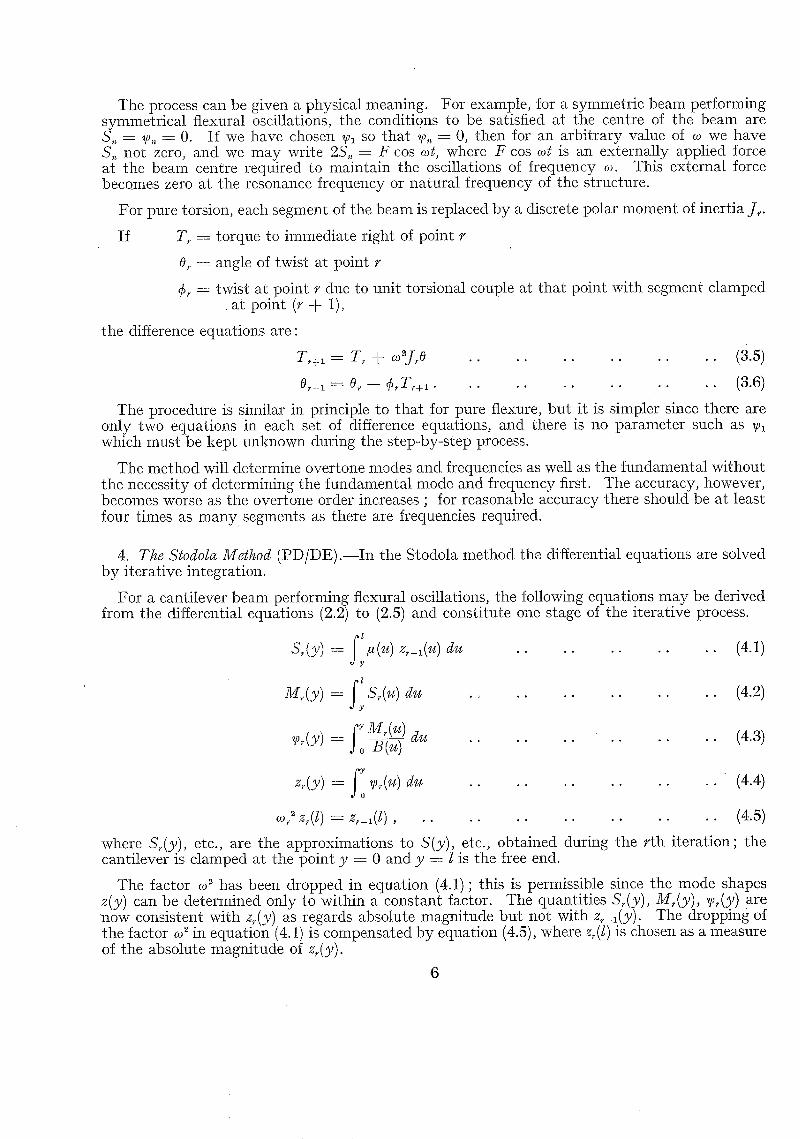
The process can be given a physical meaning. For example, for a symmetric beam performing symmetrical flexural oscillations, the conditions to be satisfied at the centre of the beam are S,~ = ~o,~ = 0. If we have chosen wl so that ~p,~ = 0, then for an arbitrary value of co we have S,~ not zero, and we may write 2S,, = F cos cot, where F cos cot is an externally applied force at the beam centre required to maintain the oscillations of frequency co. This external force becomes zero at the resonance frequency or natural frequency of the structure.

For pure torsion, each segment of the beam is replaced by a discrete polar moment of inertia J,.

If T, = torque to immediate right of point r

0r --= angle of twist at point r

¢~ : twist at point r due to unit torsional couple at that point with segment clamped at point (r -b 1),

the difference equations are:

T,+I = T, + co"],.O

0~+~ : O~ - - ¢~T,+1.

. . . . . . . . . . . . (3 .5)

. . . . . . . . . . . . (3.6) The procedure is similar in principle to that .for pure flexure, but it is simpler since there are

only two equations in each set of difference equations, and there is no parameter such as ~o~ which must be kept unknown during the step-by-step process.

The method will determine overtone modes and frequencies as well as the fundamental without the necessity of determining the fundamental mode and frequency first. The accuracy, however, becomes worse as the overtone order increases ; for reasonable accuracy there should be at least four times as m a n y segments as there are frequencies required.

4. The Stodola Method (PD/DE).- - In the Stodola method the differential equations are solved by iterative integration.

For a cantilever beam performing flexural oscillations, the following equations may be derived from the differential equations (2.2) to (2.5) and constitute one stage of the iterative process.

f l

Y

M,(y ) = S,(u) du Y

f; v , / y ) - o

(4.1)

(4.2)

(4.3)

fY z,.(y) - - ~ (u) du . . . . . . . . . . . . (4.4) 0

co2 z,(l) = z,_l(l) , . . . . . . . . . . . . . . (4.5)

where S,(y) , etc., are the approximations to S(y) , etc., obtained during the r th iteration; the cantilever is clamped at the point y = 0 and y = l is the free end.

The factor co2 has been dropped in equation (4.1); this is permissible since the mode shapes z(y) can be determined only to within a constant factor. The quantities Sdy ), M / y ) , ~ ( y ) are now consistent with z~(y) as regards absolute magnitude but not with z~_~(y). The dropping of the factor co" in equation (4.1) is compensated by equation (4.5), where z~(l) is chosen as a measure of the absolute magnitude of z d y ).

6

A shape is assumed for z0(y) ; the integrations in equations (4.1) to (4.4) are then performed, and m, determined from equation (4.5), for r = 1, 2, 3, etc., in turn. The process is repeated until two consecutive shapes zr(y) (say zN(y) and zN+dy)) agree to the required accuracy. This is then the fundamental mode and con is the fundamental frequency.

Since the integrations will have to be performed numerically, the mode shape z,.(y) will have • to be specified at a finite number of points, and the quantities S,,(y), M,,(y), ~,,(y) determined

at a finite number of points. The simplest method is to specify z /y) , M,,(y) at equidistant points ~-a 3a/2, . . (¢¢ -- ½)a, where na l, and to specify S,(y) and ~jJ,.(y) at the intermediate

points y = a, 2 a , . . . ~a. The integrations may then be replaced by simple summations, giving :

where either

o r

~ -- I

S,(ka) = Z m~z,_~[(s q- ½-)a] . . . . . . . . . . . (4.6)

f ( s + l ) ~

m , = a # [ ( s + ½)a] ,~-- 1

M , [ ( k - - { )a] ---- a Z £ ( ka ) . . . . . . . . . . . . (4.7) s = k

i M,[(s -- ½)a] . . . . . . (4.8) = a , : , B [ ( s - ½)a] . . . .

k

z,E(k + ½)a] = a ~ ~,(sa) . . . . . . . . . . . . . (4.9) s = l

Other methods of numerical integration, such as Simpson's rule, may also be used.

For beams with other end conditions an unknown parameter must be added to one or more of equations (4.1) to (4.4). This parameter is kept as an unknown during each iteration cycle and its value is determined from one of the end conditions at the end of the cycle.

The overtone modes may be found in turn by the above process if at the end of each iteration cycle the derived mode shape z~(y) is modified by adding to it multiples of each of the lower modes in such a way that the modified mode shape is orthogonal to all the lower modes. The process becomes increasingly laborious as the order of the overtone increases; a limit to the number of overtone modes and frequencies which can be accurately determined is set by the number of integration stations used.

5. Solution of Integral Equations by Numerical Integration and Collocation (PD/IE) . - -For a cantilever beam in flexure:

f' = y) z (u) d u . . . . . . . . . ( s .1 ) 0

We can derive from this equation an iteration sequence in the same way as for the Stodola method. However, since it will be impossible in practice to perform the iterations exactly, the method reduces to one using numerical integration and collocation. This replaces the integral equations by a matrix equation, which need not necessarily be solved by iteration, although the iteration method is usually the most convenient.

The collocation points will coincide with the points at which the integrands are evaluated for use in the integration formulae. Let these points be tile points y ---- y~ and let ff(y~) ---- #~, etc., and F(yr, y,) = F , .

7

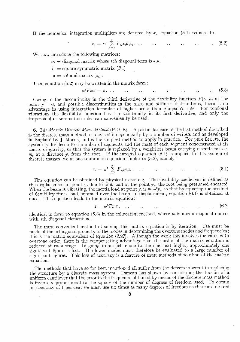
If the numerical integration multipliers are denoted by c~, equation (5.1) reduces to:

z~ = o;' ~ F,,,OCs~,Z~. . . . . . . . . . . . . (5.2) s = l

We now introduce the following matrices :

m : diagonal matrix whose sth diagonal term is e,~,

F = square symmetric matr ix IF,,]

z = column matrix [z,,] .

Then equation (5.2) may be written in the matr ix form :

~ F ~ z = z . . . . . . . . . . . . . . . . . (5.3)

Owing to the discontinuity in the third derivative of the flexibility function F ( y , u) at the point y = u, and possible discontinuities in the mass and stiffness distributions, there is no advantage in using integration formulae of higher order than Simpson's rule. For torsional vibrations the flexibility function has a discontinuity in its first derivative, and only the trapezoidal or summation rules can conveniently be used.

6. T h e M o r r i s D i scre t e M a s s M e t h o d (PD/IE) . - -A particular case of the last method described is the discrete mass method, as devised independently by a number of writers and as developed. in England by J. Morris, and is the simplest method to apply in practice. For pure flexure, the system is divided into a number of segments and the mass of each segment concentrated at its centre of gravity, so that the system is replaced by a weightless beam carrying discrete masses rn~ at a distance y~ from the root. If the integral equation (5.1) is applied to this system of discrete masses, we at once obtain an equation similar to (5.2), namely:

z, = ~ ~ F , msZ~. . . . . . . . . . . . . (6.1) s = l

This equation can be obtained by physical reasoning. The flexibility coefficient is defined as the displacement at point y~ due to unit load at the point y,, the root being presumed encastr6. When the beam is vibrating, the inertia load at point Ys is ms o)"y,, so tha t by equating the product of flexibility times load, summed over the beam, to displacement, equation (6.1) is obtained at once. This equation leads to the matrix equation:

z = c o ~ F m z , . . . . . . . . . . . . . . (6.2)

identical in form to equation (5.3) in the collocation method, where m is now a diagonal matr ix with sth diagonal element m,.

The most convenient method of solving this matr ix equation is by iteration. Use must be made of the orthogonal property of the modes ill determining the overtone modes and frequencies ; this is the matrix equivalent of equation (2.27). Although the work this involves increases with overtone order, there is the compensating advantage tha t the order of the matr ix equation is reduced at each stage. In going from each mode to the one next higher, approximately one significant figure is lost. The lower modes must therefore be evaluated to a large number of significant figures. This loss of accuracy is a feature of most methods of solution of the matr ix equation.

The methods that have so far been mentioned all suffer from the defects inherent in replacing the structure by a discrete mass system. Duncan has shown by considering the torsion of a uniform cantilever that the error in the frequency obtained by means of the discrete mass method is inversely proportional to the square of the number of degrees of freedom used. To obtain an accuracy of 1 per cent we must use six times as many degrees of freedom as there are desired

8

modes. The accuracy for flexure may be a little better. If we decide that an accuracy to within 2 per cent should be aimed at, then at least four times as many degrees of freedom as there are desired modes should be used for either flexure or torsion. In addition to ensuring the accuracy of the frequency, this should give a sufficiently large number of ordinates to determine the mode shapes with reasonable accuracy.

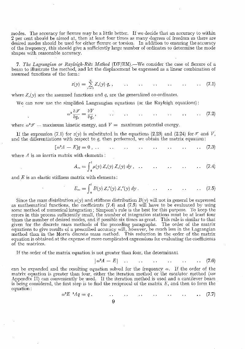
7. T h e L a g r a n g i a n or R a y l e i g h - R i t z M e t h o d (DF/EM).--We consider the case of flexure of a beam to illustrate the method, and let the displacement be expressed as a linear combination of assumed functions of the form:

= z (y) q , , . . . . . . . . . . . . (7.1) r = l

where Z r ( y ) are the assumed functions and q, are the generalized co-ordinates.

We can now use the simplified Langrangian equations (or the Rayleigh equations):

¢ j ) g m ~:- aV aq, -- aq~' . . . . . . . . . . . . . . (7.2)

where co~3 - = maximum kinetic energy, and V = maximum potential energy.

If the expression (7.1) for z ( y ) is substituted in the equations (2.23) and (2.24) forY and VI and the differentiations with respect to q,, then performed, we obtain the matrix equation:

[coM - - E J q = O , . . . . . . . . . . . . . . . . (7.3)

where A is an inertia matrix with elements :

A~, = # ( y ) Z , ( y ) Z , ( y ) d y , . . . . . . . . . . (7.4)

and E is an elastic stiffness matrix with elements :

= B ( y ) Z / ' ( y ) z,"'/y)" dy (7.5) 0

Since the mass distribution #(y) and stiffness distribution B ( y ) will not in general be expressed as mathematical functions, the coefficients (7.4) and (7.5) will have to be evaluated by using some method of numerical integration; Simpson's rule is the best for this purpose. To keep the errors in this process sufficiently small, the number of integration stations must be at least four times the number of desired modes, and if possible six times as great. This rule is similar to that given for the discrete mass methods of the preceding paragraphs. The order of the matrix equations to give results of a prescribed accuracy will, however, be much less in the Lagrangian method than in the Morris discrete mass method. This reduction in the order of the matrix equation is obtained at the expense of more complicated expressions for evaluating the coefficients of the matrices.

If the order of the matrix equation is not greater than four, the determinant

l o : A - - E [ . . . . . . . . . . . . (7.6)

can be expanded and the resulting equation solved for the frequency co. If the order of the matrix equation is greater than four, either the iteration method or the escalator method (see Appendix II) can conveniently be used. If the iteration method is used and a cantilever beam is being considered, the first step is to find the reciprocal of the matrix E, and then to form the equation :

c o 2 E - 1 A q = q . . . . . . . . . . . . . . . (7.7)

9

Alternatively, the matrix E may be expressed as the product of a lower triangular matrix and its transpose, that is:

E = LL ' . . . . . . . . . . . . . . . (7.8)

If we now write ~ = L'q, equation (7.7) becomes:

co ~ L -~ A (L-l) ' c~ = c] . . . . . . . . . . . . . . . (7.9)

We thus have to find the reciprocal of a triangular matrix, which is easier than finding the reciprocal of E.

The accuracy of the method will depend on the choice of displacement functions Z / y ) . It is most desirable that these displacement functions should satisfy not only the boundary conditions at the fixed end of the beam, but also those at the free end. The boundary conditions at the free end are given in the first place as dynamical conditions, but from them can be deduced geometric conditions: there are three different cases, depending on the ratio of flexural rigidity to mass per unit length at the free end.

Duncan has determined sets of displacement functions of polynomial form which satisfy these geometric end conditions (see Appendix I). The first four of these for a blunt-ended beam are shown in Fig. 1. For a uniform beam, accurate results for modes and frequencies can be found by using one more function than there are desired modes. For less ideal bodies, however, it appears that rather more are necessary. Even for a uniform beam, the full accuracy can be obtained only by keeping a large number of figures in the calculations. Figures are lost for the overtone modes ; there is some loss of figures for the generalized co-ordinates q, during the solution of the matrix equation and a further loss for the displacements z when the numerical values of the q~ are substituted in equation (7.1). This loss of figures would be even greater if the boundary conditions at the free end were not satisfied. The reason for the loss is that the change in shape as we pass from one displacement function to the next is only a slow one. A way of Considerably reducing it is to start the calculations not vdth the Duncan functions themselves but with linear combinations of them. In this new set of functions the first is identical with the first of the Duncan functions. For the second we combine the first two Duncan functions to give a nodal point in roughly the expected place. The third function is a combination of the first three Duncan functions to give two nodes where we expect them to be, and so on. The first three functions derived in this way are shown in Fig. 2.

For a freely supported beam, one or possibly two of the displacement functions must represent the rigid mode displacements of vertical translation or roll or both. The 'remaining displacement functions may conveniently be taken to be Duncan's displacement functions, or combinations of them ; these satisfy the conditions Z / y ) = Z / ( y ) = 0 at the point y = 0, which may be taken to be the end of an asymmetric beam or the centre of a symmetric beam.

In this case the matrix E will have a null row and null column for each rigid mode. Before the matrix equation can be expressed in the form (7.7), as required in the iteration method, the rigid mode co-ordinates will therefore have to be eliminated from the equation. This elimination will not, however, be necessary if the escalator method is used.

Displacement functions of a different kind have been introduced by Rauscher of America. Whereas Duncan's functions do not depend on the particular structure, apart from the end conditions, Rauscher's functions depend on the elastic properties of the structure, and might therefore be expected to give more accurate results.

Rauscher starts by dividing the beam into a number of segments, equal to the number of functions he wants to find, and imagines the loading curve which is typical of any one of the normal modes to be given approximately by a polygon, linear in each segment. This polygonal loading is in turn replaced by the sum of a number of triangular loadings, each triangle extending over two segments, except the tip triangle, which extends over one only (see Fig. 3). Each triangular loading is then considered in turn, and by integrating four times, introducing the stiffness distribution in the process, the displacement produced by the triangular load is obtained.

10

Since we require only the shape of the deflection curve, the height of the triangle is not in fact specified. The displacements obtained in this way for all the triangular loads then give the displacement functions. The functions found by this process for a uniform beam, with four degrees of freedom considered, are shown in Fig. 4. These functions are more alike than Duncan's functions and the risk of computational inaccuracies is therefore greater, so that it is even more necessary to combine them linearly in the way that has been described above. The second derivatives of the functions will have been found half-way through the integration process, so no disadvantage arises in not having the functions expressed in algebraic form. If there are rapid changes in the mass distribution, a refinement of the functions can be made-- ins tead of triangular loads we take loads which are the product of a triangle and the mass distribution.

What is really done in the construction of the Rauscher functions is to start with a set of arbitrary functions and obtain a set of improved functions by one round of iteration. An alternative way of obtaining functions appropriate to the particular structure considered is to start with a set of simpler algebraic functions, say functions ~ +~, and integrate to obtain improved functions.

A matrix equation identical with that of the Lagrangian method is obtained if the Galerkin method is applied to the differential equation. This is a method of making the mean error in the differential equation a minimum.

8. The Complementary Energy Method (DF/EM).--One disadvantage of the Lagrangian method is tha t the elastic coefficients depend on the second derivative of the displacement. The displace- ment functions when combined together can represent the true mode only to within a certain error. Differentiation always increases such errors so that the potential energy in the modes is given less accurately than the kinetic energy.

This differentiation is avoided in the complementary energy method, which was first developed by Grammel and reintroduced by Westergaard and Reissner. The potential energy for flexure is expressed in the form"

v = o M 2 ( y ) d y . . . . . . . . . . . (8.1)

where the bending moment M(y) is given by the double integral :

M ( y ) = du dv . . . . . . . . . (S.2) y v

If this form of the potential energy is used in applying Lagrange's equations, we obtain a matr ix equation of the form:

EA -- ~K~q = 0 , . . . . . . . . . . . . . . . . (8.3)

where the inertia coefficients A~ are the same as in the Lagrangian method (equation (7.4)) and the elastic coefficients are given by"

where f z 1

K,.s = M~(y) M~(y) dy o~(y) . . . . . . . . (8.4)

M / y ) ---- d v . . . . . . . . . . . (8.5) y v

In this matrix equation the frequency occurs in conjunction with the elastic matrix, and not with the inertia matrix as in the ordinary Lagrangian method.

11

If the elastic properties of the beam are expressed in terms of flexibility functions, the expression for the potential energy may be written in a different form by equating it to the work done by the inertia forces. If we express the displacement in the form (2.13), we than have:

(it(y) It(u) z(u) du dy (8.6) V 1 0 ) 4

2 JO 0 . . . . .

I t follows by differentiation that the coefficients K~, are given by:

K , = 0it(y) z,(y) o F(y, It(u) dy . . . . . (8.7)

This form of the expression for K,, is particularly convenient when flexibility coefficients have been determined experimentally.

This method gives more accurate frequencies than the Lagrangian method, but it has the disadvantage that more figures must be kept in the calculations to obtain this accuracy. The modes are not noticeably different, but improved mode shapes can be obtained by using the formula :

S z(°(y) = F ( y , u) It(u) z(u) du . . . . . . . . . . (8.8) 0

i f ' = s = 1 qs oF(y'u)I*(U)Z,(U) d u , . . . . . . . . (8.9)

which is derived from equations (2.13) and (7.1). The integrals under the summation sign will have already been obtained if the elastic coefficients K,, have been determined from equation (8.7), and little additional work is therefore entailed.

The above treatment applies specifically to a cantilever beam, and all the displacement functions must satisfy the condition Z(y) = Z ' ( y ) - - 0 at the clamped end. For an unsupported beam additional functions representing the rigid modes are required, but a difficulty now arises in the application of the method.

When the ordinary Lagrangian method is used, the equations obtained by differentiation with respect to the rigid mode co-ordinates are identical with equations (2.19) and (2.20), that is, they are mathematical expressions of the vanishing of the total vertical inertia force and total inertia moment. This will not be the case if the complementary energy method in the above form is used; the results obtained will be incorrect and the following modification is made.

The elastic terms in the equations of motion are now obtained by evaluating the derivatives ~V/aq~, which appear in Lagrange's equations, subject to the condition that the total force and moment equations (2.19) and (2.20) be satisfied. This is equivalent to expressing the rigid mode co-ordinates in terms of the remaining generalized co-ordinates by using equations (2.19) and (2.20), and substituting these expressions in the potential energy (8.1) or (8.6) before performing the partial differentiation.

A matrix equation identical wKh that of the complementary energy method is obtained if the Galerkin method is applied to the integral equation, making the mean error in the equation a minimum.

9. Collocatio~ with Assumed Modes (DF/ IE) .~For flexure, the displacement z(y) is again expressed in the form:

z(y) = E Z,(y) q , , . . . . . . . . . . . . (9..1) ~ '=1 '

where the Z / y ) are the assumed functions. For a cantilever beam clamped at y = 0, the functions Z,(y) must satisfy the condition

Z,(0) = Z,'(0) = 0. For this case, the expression (9.1) for z(y) is substituted in the integral equation (2.13); if the order of integration and summation is interchanged, we obtain:

i i f Z~(y) q~ = a~' q, F(y ,u ) it(u) Z~(u) du . . . . . . . (9.2) s = l . s = l 0

12

This equation cannot now'be satisfied at all points of the beam, but an approximate solution may be obtained by satisfying it at n selected collocation points yl, y~, . . . y~.

If we write:

and let

f I

G~s = F ( y ,u ) t~(u)Z,(u) d u . . . . . . . . (9.3) 0

Z~, = Z , ( y , ) . . . . . . . . . . . . . . (9.4)

G = n th order square matr ix with typical element G~s

Z = n th order square matr ix with typical element Z,,

q = matr ix column {ql, q2, • • • q,,},

we obtain the matr ix equation:

[co~G -- Z7~q = 0 . . . . . . . . . . . . . . . . . (9.5)

In the energy methods described in the last two sections the matrices in the matr ix equation are symmetric. In the collocation method, however, the matrices G and Z are not symmetric, and if matr ix iteration is used the calculation of the overtone modes and frequencies is a little more troublesome• The accuracy is in general not quite as good as in the energy methods, but may be better if t he collocation points happen to have been chosen fortunately.

For an unsupported beam, two of the displacement functions must represent the rigid modes of vertical translation and roll. The modification (2.17) is now made to the left-hand side of the integral equation (2.13) and equation (9.2) is altered accordingly. This equation is now satisfied at only (n -- 2) collocation points, and the deficiency in the number of equations is made up by satisfying equations (2.19) and (2.20) which equate the total inertia force and total inertia moment to zero. A matrix equation of similar form to equation (9.5) is again obtained, but the matr ix corresponding to Z has two null rows and two null columns.

10. N u m e r i c a l E x a m p l e C o m p a r i n g the V a r i o u s M e t h o d s . - - T h e following results for the flexural modes of a tapered beam of constant width, with depth at the tip one fifth of the depth at the root, are taken from a report by Siddall and Isakson 1.

M e t h o d

L a g r a n g e . . . . . . . . . . . .

C o m p l e m e n t a r y e n e r g y . . . . . . . .

C o m p l e m e n t a r y e n e r g y . . . . . . . .

D i s c r e t e m a s s . . . . . . . . . . . .

M y k l e s t a d . . . . . . . . . . . .

D e g r e e s of M o d e s f r e e d o m

P e r c e n t e r r o r i n f r e q u e n c y

•. D u n c a n

. . D u n c a n (

• . R a u s e h e r

2 3

2 3

2

5

11

1st

+ 2 " 4 + 0"45

- - 0 " 0 5 - - 0 " 0 9

- - 0 " 0 9

- - 0 " 0 9

- - 0 " 0 2

2 n d 3 r d

+ 4 2 . 0 + 9 . 3 + 6 6 - 2

+ 4 . 3 - - 0 . 6 5 - - 1 2 . 2

- - 1 . 8

+ 2 . 8 2

+ 0 . 6 9

If an accuracy to within 2 per cent is our objective, then the first line shows tha t the Lagrangian method with two of Duncan's functions almost gives this accuracy for the fundamental frequency. For the first overtone frequency, however, at least four of Duncan's functions would be required ; if we make the reasonable assumption that the errors in this frequency with increasing number

13

of functions form a geometric sequence*, then four functions would be sufficient to give an error of not more than 2 per cent. This suggests that the Lagrangian method in conjunction with Duncan's functions will give sufficiently accurate results if the number of assumed functions is two greater than the number of desired modes. If Duncan's modes are used in the complementary energy method we see that the number of frequencies given accurately is one less than the number of assumed modes. If the modes are replaced by Rauscher's modes, there is a further improve- meri t-- two frequencies are given to within an accuracy of 2 per cent when only two displacement functions are used.

For the Morris discrete mass method, however, even with five masses the second frequency is nearly 3 per cent in error. The Myklestad method will give errors which are very little different from those of the Morris discrete mass method; with 11 masses the first two frequencies have errors almost the same as the complementary energy method using three of Duncan's functions.

One point which may be noted is that while the error in the Lagrangian method is always positive (that is, the calculated frequencies are too high), the error in the complementary energy method may be positive or negative.

The mode shapes for the fundamental mode are quite good in every case. Fig. 5 shows the shape of the first overtone mode when two degrees of freedom are used, compared with the exact mode shape. The Rauscher functions give a better mode shape than do Duncan's functions; there is little difference between the Lagrangian and complementary energy methods, but the mode shape obtained by the latter method can be improved by integration, as has been indicated above. There is then little difference between the mode obtained and the true mode in this particular case.

The best method to be used for a particular problem will depend on the calculating aids available. If desk machines are used, it is recommended by the author that in general the Lagrangian method should be used in conjunction with displacement functions of the Rauscher type, but if the flexibility function is known for the system the complementary energy method with Duncan's modes should be used, as in this case the modes can be improved without difficulty. This would enable a given accuracy to be obtained with the minimum number of degrees of freedom. This saving of work is offset by the increased work involved in setting up the matr ix equations as compared with the Lagrangian method ill terms of Duncan's displacement functions, and especially compared with the discrete mass methods. In addition, greater care is needed to avoid computational errors. However, the reduction in the order of the matr ix equation is the most important consideration, and in all probability there is a saving of effort.

If a digital computer were available, however, it would be important to keep the programming as simple as possible even though the number of degrees of freedom was relatively large. Since standard sub-programmes exist for the manipulation of matrices, the Morris discrete mass method would be the best method to use.

One method which has not been mentioned is a method devised by Duncan based on Lagrange's equations which makes use of the orthogonal properties of the modes in such a way that only two degrees of freedom need be considered at any stage of the calculation, whichever mode is being evaluated. The solution of the matr ix equation is therefore quite simple, and the method is well suited for desk-machine calculation. There is an accumulation of error as the overtone order increases, additional to that in the ordinary Lagrangian method, but when applied to a uniform beam good accuracy is obtained for the first three frequencies.

11. Coupled Flexure-Torsiora.--When the coupling between flexure and torsion has to be taken into account, some assumption has to be made about a flexural axis. Suppose tha t some line can be found in the structure such that a couple applied at any point about the tangent to the

* The error given by tile Lagrangian method decreases much more rapidly with the number of degrees of freedom than does the error given by the discrete mass method.

14

line produces no flexural curvature of the line at tha t point. If this line (the locus of flexural centres) is straight and normal to the line of clamping at the root (normal to the centre-line for an aircraft wing), the line is termed a flexural axis.

The basic equations of section 2 need some modification for this case.

(a) Differential Equat ions . - -Equat ions (2.1) and (2.8) are replaced by the equations:

a~ I a~ t ay~ B(y) ay2t = ~2{~(y) ~(y) + ~(y) o ( y ) } , . . . . . . . . (11.1)

d c ( y ) , , y = , . . . . . . . . (11.2)

where ~(y) = mass moment about flexural axis per unit length.

These equations must now be considered as a pair instead of separately.

Similarly, equations (2.2) and (2.9) are replaced by the equations:

dS ay - ~{,.(y) z ( y ) + ~(y) o ( y ) } , . . . . . . . . (11.3)

aT dy -- m={~(y) z(y) + ~(y) o(y)} . . . . . . . . . (11.4)

Equations (2.8) to (2.5) and (2.10) remain unaltered.

(b) The Integral Equat ion. - -Equat ions (2.13) and (2.15) are replaced by the pair of equations:

~(y) = ~ ~ (y ,~ ) {~(~) ~(~) + ~(~) o(~)} a~ . . . . . (11.5) o

o(y) = ~ ~(y ,~) {~(~) ~(~) + ~(~) o(~)} a~ . . . . . (11.6) 0

If a straight flexural axis in the above sense does not exist, a more general form of these equations may be used, provided that sections normal to the beam may still be assumed not to distort. We can then write:

z ( y ) = ~o ~ F ( y , ~) {~(u) ~(~) + ~(u) 0(~)} au 0

Y + co ~ T(y , u) {$(u) z(u) + z(u) 0(u)} du , . . . . (11.7) 0

Y o(y) = ~ ~(u, y) {~(~) z(u) + ~(u) 0(u)} au 0

+ ~ ~(y, u) {~(u) ~(u) + ~(~) 0(u)} au , .. .. (11.8) 0

where the axis of y is now taken as any convenient axis along the length of the structure, and the new influence function is defined as:

g~(y, u) = displacement at point y on axis due to unit torsional couple at point u

N(u, y) = angle of twist at section y due to unit load at point u on axis.

The functions F(y , u) and # (y, u) have the same physical meaning as before except that they are referred to the reference axis instead of to the flexural axis. They will not now, however, be defined by equations (2.14) and (2.16). The three functions F, ~ and N could be measured experimentally, and can in principle take account of the shear effects.

15

Equations (2.19) to (2.21), which express the fact that the total inertia force and moments are zero, are replaced by the equations"

f l + = 0 . . . . . . . . . (11.9)

f ~ { ~ ( ~ ) ~ ( ~ ) + ~ ( ~ ) o ( ~ ) } ~ a ~ = o , . . . . . . . . (11.1o) 0

0{~(u) z(u) + ~(u) 0(u)} du = 0 . . . . . . . . . (11.11)

These equations apply whether tile axis of y is the flexural axis or not.

(c) Rayleigh's E q u a t i o n s . - - T h e expressions (2.23) and (2.25) for Y are now replaced by the single equation :

9" = ½ o{tt(y) z2(y) + 2~(y) z(y) O(y) + n(y) O~(y)} dy , . . . . (11.12)

and the expressions (2.24) and (2.26) for V are replaced by the single equation"

1;1 I V = ~" o B(y ) \dyU + C(y) \dv]~ dy . . . . . . . . . (11.13)

The methods described in the previous sections can now readily be generalized by using the above equations. In the discrete mass methods the system is replaced by a weightless beam carrying discrete masses and moments of inertia at the end of a finite number of transverse rigid arms. In the Myklestad method six difference equations have now to be considered together, equations (3.1) and (3.5) being suitably modified. Two unknowns 01 and ~/J1, instead of only one, have to be carried through each stage of the work and determined by the boundary conditions at the far end. Similarly in the Stodola method a set of six integrals has to be considered at each. iteration step. In the collocation and Morris discrete mass methods, equations (5.2) and (6.1) are replaced by a pair of summation equations, and the matrix equation corresponding to (5.3) or (6.2) can be readily derived.

In the methods using displacement functions we express the flexural and torsional displacements by the pair of equations"

z(y) = ~ Z , (y ) q~, . . . . . . . . . . . . . . (11.14) s = l

o ( y ) - - ~ o s ( y )x . . . . . . . . . . . . . . . . . (11.15) S = I

where Zs(y), O,(y) are the flexural and torsional displacement functions respectively, and qs, xs the corresponding generalized co-ordinates. The number of flexural freedoms n and torsional freedoms v must be the same in the collocation method, but can be different in the energy methods. The resulting matrix equation can be written in partitioned form, the partition lines dividing each matrix into four sub-matrices of which the two diagonal sub-matrices are pure flexure and pure torsion matrices and the two remaining sub-matrices contain the coupling I terms. In the matrices corresponding to Z of the collocation method and E of the Lagranglan method, the coupling sub-matrices are null, but in the complementary energy method there are no zero elements.

I t may sometimes be convenient to take assumed modes each of which are part ly flexural and part ly torsional. Then instead of (11.14) and (11.15) we write"

2n

z(y) = Z z:(y) qs, . . . . . . . . . . . . . . (11.16) s = l

o(y) = ~, O~(y) q , , . . . . . . . . . . . . . . (11.17) S = I

16

so tha{ :the motion in each degree of freedon qs is represented b y t h e pair of displacement functiong Zs(y) and O/y). When these equations are used, the expressions for the elements of the matrices in the matr ix equation are more complicated than when the simpler equations (11.14) and (11.15) are used. A particular case when equations (11.16) and (11.17) would be appropriate is when the normal modes of a structure have been found and the normal modes of the structure af ter some modification of it are required. The normal modes of the original structure could then conveniently be used as assumed modes in the calculations.

12. Com])lex Structures.--Except for the integral equation in the form (11.7) and (11.8), t he discussion of the last section assumed that there will be a straight flexural axis, but in general this will not be the case. I f we consider a swept-back wing, the locus of flexural centres may be straight for most of the span, but it will certainly be curved near tile wing root and will meet the centre-line at right angles (see Fig. 6). In dealing With such a wing the simplest approximation is to assume tha t the root triangle ABC is rigid. A better approximation is to assume a shape for- the deflection of the curved part of the line of flexural centres, say parabolic. If the line AC and all other lines radiating from A in the root triangle are assumed to remain rigid, the mot ion of all points in the triangular area is prescribed. Flexural and torsional displacement functions may then be assumed relative to the root triangle for the remainder of the structure and the equations of motion set up.

In the more general case, where the locus of flexural centres is everywhere curved, it may be possible to approximate to it by a polygonal curve. Each straight part of the polygon is t r ea ted separately and certain continuity relations satisfied at the junction of consecutive parts. However, it is possible to treat the problem properly in this case only if flexibility coefficients are known at various points over the surface, and the same applies if the distortion of chordwise sections .is not sufficiently small, as may be the case for wings of Small aspect ratio. In this case the motion of the wing is described not by a combination of flexure and torsion but by t h e displacement of points over the whole wing area. The integral equation may then be wri t ten:

z(,, y) = f f F(x, y.. v) v) v) ev . . . . . . . (re.l),

where p(x, y) = mass per unit area

F(x,y," u, v) = deflection at point (x, y) due to unit load at point (u, v) = F(u, v ;x , y).

This equation could be solved by the Morris discrete mass method, collocation with assumed/ modes or the complementary energy method. The discrete mass method would be the simplest in practice. The wing surface is divided into a number of small areas and the mass in each area is concentrated at its centre of gravity. The matr ix equation for frequency and displacement can then be set up in a way similar to tha t for a simple beam. Flexibili ty coefficients are required for each of these centres of gravity, giving the deflection at one centre of gravi ty due to unit load at each of the others in turn. D. Williams 9~ has developed a method suitable for a digitaI computer by means of which these flexibility coefficients can be calculated.

Displacement functions for wings of this general type for use in either the collocation or complementary energy methods can be obtained by a generalization of Rauscher's method. Fig. 7 shows a delta wing divided into squares (the number of chordwise areas shown are probably more than are necessary). Instead of obtaining the deflections due to a triangular load, we must now consider a pyramid load covering four adjacent squares with apex at the common point of t he squares, and determine the deflected shape of the wing under such a load.

13. Complete Aircraft.--When the frequencies and modes of a complete aircraft are required, a convenient method is first to obtain separately by a matr ix method the frequencies and modes. of the wings encastr6 at the root ari~d-of-the fuselage-tail combination encastre at its junct ion

17 (68984) B-

with the wing. _matrix form"

The equation for the complete system may then be written in the partit ioned

i ] . . . . . ,131,

where the matrices W, F and R represent the wing, fuselage-tail combination and rigid mode terms respectively. The rigid freedoms will be vertical translation and pitch for symmetric motion, and roll, lateral displacement and yaw for antisymmetric motion. The matrices ~. and represent the coupling terms arising from the rigid freedoms. We first consider one rigid freedom only which is represented by one row and one column of the matr ix in (13.1). Then from the known solutions of the fixed root equations:

Wq~ = O, Fq~ = 0 . . . . . . . . . . . . . . . (13.2)

we can by using the escalator method (see Appendix II) obtain an equation for frequency in the form"

• c , - - d , 2 - - e - - f Z , . . . . . . . . . . ( 1 3 . 3 )

where 2 = 1/~o ~. This equation can be solved for 2 by a method of successive approximations, and the elements of the column matrices q~, ql and q~ are then obtained from expressions of similar form to the left-hand side of the equation. A second rigid freedom is now added and an equation of the form (13.3) is again used, where the quantities a to f now depend on the solution wi th one rigid freedom. If there are three rigid freedoms, the process is again repeated.

The escalator method is equivalent to setting up a new matrix equation in terms of the fixed root modes of the wing and the fuselage-tail combination which have already been determined, but the method does this systematically and one does not have to think of it consciously.

The escalator method cannot, however, be used if the complementary energy method is used to set up the matr ix equation. This is because of the dffficulty introduced by the rigid freedoms mentioned at the end of section 8. When the modified procedure described there is adopted, it is found that the matrices W and F of equation (13.1) are different from the matrices W and F in the fixed root equations (13.2), and in addition equation (13.1) does not contain any null

sub-matrices. The best procedure is therefore to use the fixed root modes as new assumed modes in setting up the equations for the complete aircraft, using the ordinary Lagrangian method to do so. The inertia coefficients are readily obtained from differentiation of the kinetic energy, and the elastic terms then follow at once since the fixed root natural frequencies are known. With one rigid mode we then obtain at once an equation of the form (13.3); when further rigid modes are added we can again use the escalator method. This method could also be used if the fixed root modes of the wing and fuselage-tail combination have been obtained by either the Myklestad or the Stodola method.

The procedure described above of calculating the fixed root frequencies and modes first and using these results in obtaining the frequencies and modes of the complete aircraft is certainly advisable if desk machines are used for the calculations. When an electronic computer is used, :on ~he other hand, the saving in calculation time compared With that required to solve equation (13.1) dire.ctly would probably be insufficient to compensate for the complication in the programming. Even in this case, however, it might still be advisable to adopt the above procedure, for there are grounds for believing tha t the fixed root modes are better suited for use in flutter .calculations than are those of the complete aircraft. The modes of the complete aircraft would still have to be calculated, for it is only by a subsequent comparison of them with the resonance- t e s t modes tha t the calculations could be checked.

18

A

B(y)

c(y) E

r(y,

Fr s

F

F(x, y ; u, v)

fr

G

g,

h,

I

]r K

1

L

M ( y )

M,

Mr(y)

N4

q4

q

qr

s(y) St(V) T(y)

9 -

g , V

NOTATION

: [A~,l Square matr ix of inertia coefficients

Flexural rigidity, or fiexural stiffness per unit length. Young's modulus times second moment of area of section about neutral axis

Torsional rigidity, or torsional stiffness per unit length

----- [E,,] Square matrix of elastic stiffness coefficients

Flexibility or influence function. Displacement at point y due to unit load at point u

= F(y,, y,) Flexibility coefficient

= [F,s~ Square matr ix of flexibility coefficients

Displacement at point (x, y) due to unit load at point (u, v)

Flexibility coefficient for flexure of r th segment of beam (displacement due to unit load)

= [G,,I Square matr ix of coefficients for method of collocation with assumed modes

Flexibility coefficient for flexure of r th segment of beam (slope due to unit load)

Flexibility coefficient for flexure of r th segment of beam (slope due to unit couple)

Unit matrix

Polar inertia of r th segment of beam

= [K,~ Square matrix of elastic coefficients in the complementary energy method (dimensions stiffness divided by frequency ~)

Length of beam

Lower triangular matr ix

Bending moment at point y

= M(y,)

Either r th iterate to bending moment or bending moment due to loading ~(y) Zr(y)

Discrete mass at point Yr

Diagonal matr ix with elements m, or ¢,t* (Y,)

Number of degrees of freedom

Column matrix with elements q,

Generalized co-ordinate associated with r th degree of freedom

Sheafing force at point y

r th iterate to shearing force

Torque at point y

(1/~o 2) times maximum kinetic energy

Integration variables

19 (68984) B *

V

X

Y

Z,

Z

z,(y) Zrs

Z

~X r

rl

o(y) O,

o (y) o,(y) .(y)

2

7~

+(y) p (x, y)

u)

60

OJ r

NOTATI ON--continued

Maximum potential energy

Transverse co-ordinate

Co-ordinate along length of beam

Vertical displacement of beam at point y

z(y ) Column matrix with elements z,

Either flexural displacement in r th normal mode or r th iterate to the flexural displacement

Displacement function for flexure

Square matrix [Z,,J

Numerical integration constant

y/Z

Torsional displacement

O(y~)

Torsional displacement in r th normal mode

Displacement function for torsion

Moment of inertia about reference axis per unit length

Mass per unit length

Number of torsional degrees of freedom

Mass moment about reference axis per unit length

Mass per unit area

Flexibility function for torsion. Twist at point y due to unit torque at point u

Flexibili ty coefficient for torsion of r th segment of beam (twist due to unit torque)

Function of coupling flexibilities. Displacement at point y due to unit torque at point u

Frequency of vibration in radians per second

Either r th natural frequency or r th iterate to the frequency

A superscript dash denotes the derivative of a function or the transpose of a matrix.

The origin y = 0 is taken to be the clamped end of a cantilever beam, one free end of an asymmetric unsupported beam, and the centre of a symmetric unsupported beam.

20

REFERENCES

Bibliography of Methods of Determination of Normal Vibration Modes ct~¢d Frequencies

A. General.

1 J.W. Siddall and G. Isakson. .

2 A . I . van de Vooren . . . .

3 L. Collatz . . . . . .

Approximate analytical methods for determining ilatural modes and frequencies of vibration. M.I.T. Report Contract N5 ori-07833. Project NR-035-259. January, 1951.

Theory and practice of flutter calculations for systems with many degrees of freedom. Eduard Ijdo N.V. 1952.

Eigenwer@robleme u~d ihre numerische Beha~dlu~g. Akademische Verlags- gesellschaft. 1945.

B. Holzer-Myklestad Method 4 H. Holzer . . . . . .

5 N .O . Myldestad . . . .

6 W . P . Targoff . . . . . .

7 A . I . Bellin . . . . . .

8 J . A . Fay . . . . . .

9 W . T . Thompson . . . . .

10 W . T . Thompson . . . .

Die Berechnul,g der Drehschwi~,gu~gen. J. Springer. 1921.

Vibratio,~ A~zalysis. McGraw-Hill. 1944.

The associated matrices of bending and coupled bending torsion vibration. J. Aer. Sci. Vol. 14. No. 10. p. 579. October, 1947.

Determination of the natural frequencies and the bending vibration of beams. J. A~bp. Mech. Vol. 14. No. 1. p. A-1. March, 1947.

A method of determining the natural frequencies of bending vibration of uniform beams. J. Am. Soc. Nav. Eng. Vol. 60. p. 316. August, 1948.

Matrix solution for the vibration of non-uniform beams. J. App. Mech., Vol. 17. No. 3. p. 337. September, 1950. '

A note of tabular methods for flexuraI vibrations. J. Ae. Sci. Vol. 20. No. 1. January, 1953.

C.

11

12

13

14

15

Stodola Method J. P. Den Hartog . . . .

J. C. Houbolt ~md R. A. Anderson.

H. E. Fettis . . . . . .

L. Beskin and R. M. Rosenberg

13/I. L. Gossard

(See also.Ref. 34).

Mechanical Vibrations. p. 194. McGraw-Hill. 1947.

Calculation of uncoupled modes and frequencies in bending and torsion of non-uniform beams. N.A.C.A.T.N. 1522. February, 1948.

The calculation of coupled modes of vibration by the Stodola method. J. Ae. Sci. Vol. !6. No. 5. p. 259. May, 1949.

Higher modes of vibration by a method of sweeping. J. Ae. Sci. Vol. 13. No. 11. p. 597. November, 1946.

An iterative transformation procedure for numerical solution of flutter and similar characteristic-value problems. N.A.C.A.T.N. 2346. May, 1951.

D. Morris Method. 16 J. Morris and I. T. Minhinnick

17 J. Morris and D. Morrison . .

18 J . Morris and G. S. Green ..

19 R.W. Traill-Nash . . . .

20 R . W . Traill-Nash . . . .

21 W . J . Duncan

(See also Ref. 85).

The calculation of the natural frequencies and modes of vibration of aeroplane wings. R. & M. 1928. April, 1940.

The rolling vibrations of an aircraft. R. & M. 2290. August, 1945.

The pitching vibrations of an aircraft. R. & M. 2291. October, 1945.

The symmetric vibrations of aircraft. Aero. Quart. Vol. I I I . Part I. p. 1. May, 1951.

The antisymmetric vibrations of aircraft. Aero. Quart. Vol. I I I . Part I I . p. 145. September, 1951.

A critical examination of the representation of massive and elastic bodies by systems of rigid masses elastically connected. Quart. J. Mech. App. Maths. Vol. V. Pt. 1. p. 97. March, 1952.

21

R E F E R E N C ES--continued

E. Collocation of Integral Equation with Numerical Integration.

22 W . T . White . . . . . . All integral equation approach to the problem of vibrating beams. J. Frank. Inst. Vol. 245. p. 25. Jan., 1948. p. 117. February, 1948.

23 F . D . Murnaghen . . . . A~@lied Mathematics. J. Wiley & Sons. p. 247. 1948.

24 F .S . Shaw . . . . . . The approximate numerical solution of the non-homogeneous linear Fredholm integral equation by relaxation methods. Quart. App. Math'. Vol. VI. No. 1. p. 69. April, 1948.

F.

25

26 M. Rauscher . . . . . .

27 ,1. H. Greidanus and A. I. van de Vooren.

28 A. Mendelson and S. Gendle1:..

Collocation of Integral Equation with Assumed Functions.

P. D. Crout . . . . . . An application of polynomial approximation to the solution of integral equations arising in physical problems. J. Math. Phys. Vol. 19. p. 34. 1940.

Station functions and air density variations in flutter analysis. J: Ae. Sci. Vol. 16. No. 6. p. 345. June, 1949.

Station functions in flutter analysis. J. Ae. Sei. Vol. 17. p. 178. 1950.

Analytical determination of coupled bending-torsion vibrations of cantilever beams by means of station functions. N.A.C.A.T.N. 2185. September, 1950.

G. Lagrangian Method. 29 G. Temple and W. G. Bickley Rayleigh's Principle. 1933.

30 W. Ritz . . . . . . 13bet eine neue Methode zur L6sung gewisser Variationsprobleme der MathematischenPhysik. J.r.a.M. Vol. 135. 1909.

31 N. Kryloff . . . . . . Les m6thodes de solution approch6e d e s probl~mes de la physique mathematique. Gauthier-Villars. 1931.

32 S. Timoshenko . . . . Vibration Problems in Engineering. Vail Nostrand Co. 1937.

33 T. yon I(~rm~n and M. A. Biot Mathematical Methods in Engineering. McGraw-Hill. 1940.

34 W.J .DuncanandD.D.Lindsay Methods for calculating the frequencies of overtones. R. & M. 1888. September, 1939.

35 W . J . Duncan . . . . Mechanical admittances and their applications to oscillation problems. R. & M. 2000. March, 1946.

36 C.F . Garland . . . . . . The normal modes of vibration of beams having collinear elastic and mass axes. J. Apj). Mech. p. A-97. September, 1940.

37 R. A. Anderson and J . C . Determination of coupled and uncoupled modes and frequencies of natural Houbolt. vibration of swept and unswept wings from uniform cantilever modes.

N.A.C.A.T.N. 1747. 1948.

H. Complementary Energy Method. 38 R. Grammel . . . . . . Ein neues Verfahren zur L6sung technischer Eigenwertprobleme. Ing.-

Arch. Vol. 10. p. 35. 1939.

39 H .M. Westergaard . . . . On the method of complementary energy. Proc. Am. Soc. Civ. Eng. Vol. 67. No. 2. p. 199. February, 1941.

40 E. Reissner . . . . . . Note on the method of complementary energy. J. Math. Phys., Vol. 27. p. 159. 1948.

41 t~. Reissner . . . . . . Complementary energy procedure for flutter calculations. J. Ae. Sci. Vol. 16. No. 5. p. 316. May, 1949.

42 P .A. Libby and R. C. S a n e r . . Comparison of the Rayleigh-Ritz and complementary energy methods in vibration analysis . .J . Ae. Sci. Vol. 16. No. 11. p. 700. November, 1949.

4 3 A . I . van de Vooren and J . H . Complementary energy method in vibration analysis. J. Ae. Sci. Vol. 17. Greidanus. No. 7. p. 454. July, 1950.

22

J. Galerkin Method. 44 W . J . Duncan

45 W . J . Duncan

R E F E R E N C ES--continued

Galerkin's method in mechanics and differential equations. R. & M. 1798. 1938.

The principles of the Galerkin method. R. & M. 1848. September, 1939.

K. Choice of Displacement Functions. Duncan's polynomial functions (see Refs. 34, 35).

Rauscher's functions (see Ref. 26).

Other functions (see Refs. 37, 88).

t .

46

47

48

49

50

5I

52

53

54

55

56

57

58

59

60

61

62

63

Solution of Matrix Equation. (a) Matrix Iteration.

W. J. Duncan and A. R. Collar

R. A. Frazer, W. J. Duncan and A. R. Collar.

A. R. Collar . . . . . .

W. M. Kincaid . . . .

H. A. Jahn . . . . . .

I-I. Wielandt . . . . . .

(b) The Escalator Method. J. Morris and J. W. Head ..

j . Morris . . . . . .

B. Vinograde . . . . . .

L . F o x . . . . . . . .

(c) Relaxation Method. R. V, Southwell . . . .

L. Fox . . . . . . . .

J. L. B. Cooper

(d) Errors. L. B. Tnckerman

J. von Neumann

A. M. Turing ..

R. Redheffer ..

J. M. Souriau ..

A method for the solution of oscillation problems by matrices. Vol. 17. No. 115. p. 865. May, 1934.

Elementary Matrices. Cambridge. 1938.

Phil. Mag.

Note on the computation of the sub-dominant latent roots of a matrix. A.R.C. 8074. September, 1944.

Numerical methods for finding characteristic roots and vectors of matrices. Quart. App. Math. Vol. 5: No. 3. p. 320. October, 1947.

Improvement of an approximate set of latent roots and modal columns of a matr ix by a method akin to those of classical perturbation theory. Quart. J. Mech. App. Math. Vol. 1. p. 131. June, 1948.

Determination of higher eigenvalues by broken iteration. Z.W.B. UM 3177. 1944. M.A.P. Translation : A.R.C. 11,608. August, 1946.

The escalator process for the solution of Lagrangian frequency equations. Phil. Mag. Vol. 35. No. 350. p. 735. November, 1944.

The Escalator Process. Chapman & Hall. 1947.

Note on the escalator method. Proe. Am. Math. Soc. p. 162. April, 1950. Also A.R.C. 13,502. November, 1950.

Escalator methods for latent roots. Quart. J. Mech. App. Maths. Vol. V. Pt. 1. p. 97. March, 1952.

Relaxation methods in engineering science. 1940.

A short account of relaxation methods. Quart. J. Mech. App. Math. Vol. I. Part 3. p. 253. September, 1948.

The solution of natural frequency equations by relaxation methods. Quart. App. Math. Vol. VI. No. 2. p. 179. July, 1948.

On the mathematically significant figures in the solution of simultaneous linear equations. Ann. Math. Star. Vol. x n . No.3. p.307. September, 1941.

Numerical inverting of matrices of high order. Bull. Am. Math. Soc. Vol. 53. p. 1021. 1947.

Rounding off errors in matrix processes. Quart. J. Mech. App. Math. Vol. I. Part 3. p. 287. September, 1948.

Errors in simultaneous linear equations. Quart. App. Math. Vol. VI. No. 3. p. 342. October, 1948.

Th4orie des erreurs en calcul matriciel. La Recherche Aeronautique. No. 19. p. 41. January, 1951.

23 (68984) B **

M. Apy~lication of Computation Aids 64 R . R . M . Mallock . . . .

65 G. Kind-Schaad . . . . .

66 G. Kind-Schaad . . . .

67 S. Bergmann . . . . . .

68 G. D. McCann and R. H. MacNeal.

R E F E R E N C ES--conEinued

Determination of latent roots by means of the Mallock Calculating Machine. R.A.E. Vib. 10. A.R.C. 9244. October, 1945.

L6sung yon Eigenwertproblemen mittels Lochkartmaschinen. Schweiz. Arch. fCir angewa~dte Wissensehaft und Technih. January, 1947.

LSsung der Schwingungsgleichungen durch Lochkartenverfahren. Bericht FP 3119/21. Swiss Fed. Air. Works. March, 1946.

Punch card machine methods applied to the solution of the torsion problem. Quart. A~p. Ma~h. Vol. V. No. 1. p. 69. April, 1947.

Beam-vibration analysis with the electric analog computer. J. App. Mech. Vol. 17. No. 1. p. 13. March, 1950.

N. Shear and Rotary Inertia Effects. 69 R . H . Scanlan . . . .

70 H . E . Fettis . . . . . .

71 E . T . Kruszewski . . . .

72 J. C. Houbolt and R. A. Anderson.

73 D. Williams . . . . . .

74 I). Williams . . . . . .

75 E . H . Mansfield . . . .

76 R. Chaplin . . . . . .

77 E. Saibel . . . . . .

Miscellaneous 78 I). Williams . . . . . .

79 H. Wit tmeyer . . . .

80 E . H . Mansfield . . . .

81 N .S . Heaps . . . . . .

82 R. Courant . . . . . .

83 H.D. Conway ....

84 E . T . Kruszewski and J. C. Houbolt.

85 W . J . Duncan and H..M. Lyon

A note on transverse bending of beams having both translating and rotating mass elements. ,[. Ae. Sci. Vol. 15. No. 7. p. 425. July, 1948.

Note on the effect of rotary inertia on higher modes of vibration. J. Ae. Sci. Vol. 16. No. 7. p. 445. July, 1949.

Effect of transverse shear and rotary inertia on the natural frequency of a uniform beam. N.A.C.A.T.N. 1909. July, 1949.

Effect of shear lag on bending vibration of box beams. N.A.C.A.T.N. 1583. May, 1948.

Note on the distortion characteristics of swept and cranked Wings in relation to flutter and other aeroelastic phenomena. R.A.E. Tech. Note Struct. 44. A.R.C. 12572. July, 1949.

A simple method of allowing for shear deflections in calculating the vibration modes and frequencies of structures. R.A.E. Report Struct. 49. A.R.C. 12,676. August, 1949.

The theory of torsional vibrations of a four-boom thin-walled cylinder of rectangular cross-section. R. & M. 2867. March, 1951.

The natural frequencies of vibration of prismatic blades. C.P. 95. July, 1951.

Vibration frequencies of continuous beams. J. Ae. Sci. Vol. II. No~ 1. p. 88. January, 1944.

Rapid estimates of the higher natural frequencies and modes of beams. R.A.E. Tech. Note Struct. 18. A.R.C. 11,649. June, 1948.

A simple method for the approximate computation of all the natural torsional frequencies of a member with variable cross-section. R. Inst. Tech. Stockholm. Tech. Note K T H - A E R 0 TN. 13. 1951.

Elasticity of a sheet reinforced by stringers and skew ribs with applications to swept wings. R. & M. 2758. December, 1949.

The vibrations of a swept wing. C.P. 141. April, 1952.

Variational methods for the solution of problems of equilibrium and vibrations. Bull. Am. Malh. Soc. Vol. 49. p. 1. January, 1943.

Calculation of the frequencies of truncated pyramids. Aim. Eng. Vol. 20. No. 231. p. 148. May, 1948.

The calculation of modes and frequencies of a modified structure from those of the unmodified structure. N.A.C.A.T.N. 2132. July, 1950.

TorsionM oscillations of a cantilever when the stiffness is of composite origin. R. & M. 1809. November, 1937.

24,

Miscellaneous--continued 86 H . R . Lawrence . . . .

87 A . T . Zahorski . . . .

88 H . E . Fettis . . . . . .

89 R .A . Frazer, W. P. Jones and S. W. Skan.

90 I. Malkin . . . . . .

91 R. N. Arnold and G. B. Warburton.

92 D. Williams . . . . . .

93 D. Williams . . . . . .

94 S. Levy . . . . . .

95 S. Levy . . . . . .

96 W . F . Cahill and S. Levy . .

97 B.M. Fraeys de Veubeke . .

R E F E R E N C E S - - c o n t i n u e d

The dynamics of a swept wing. J. Ae. Sci. Vol. 14. No. 11. p. 643. November, 1947.

Free vibrations of a sweptback wing. J. Ae. Sci. Vol. 14. No. 12. p. 683 December, 1947.

Torsional vibration modes of tapered bars. J. A#~b. Mech. p. 220. June, 1952.

Approximations to functions and to the solutions of differential equations. R. & M. 1799. 1937.

On a generalization of Kirchoff's theory of transverse plate vibrations in tile vibration problem of steam turbine disks. J. Franklin Inst. Vol. 234. p. 355. 1942.

The flexural vibrations of thin cylinders. Inst. Mech. Eng. A.R.C. 15,127. August, 1952.

Recent developments in the structural approach to aeroelastic problems. J. R. Aer. Soc. June, 1954.

A general method (depending on the aid of a digital computer) for deriving the influence coefficients of aeroplane wings. R.A.E. Report Strnct. 168. A.R.C. 17,438. November, 1954.

Computation of influence coefficients for aircraft structures with dis- continuities and sweepback. J. Ae. Sci. Vol. 14. No. 10. p. 547. October, 1947.

Structural analysis and influence coefficients for delta wings. J. Ae. Sci. Vol. 20. No. 7. p. 449. July, 1953.

Computation of vibration modes and frequencies on SEAC. J. Ae. Sci. Vol. 22. No. 12. p. 837. December, 1955.

Iteration in semi-definite eigenvalue problems. J. Ae. Sci. Vol. 22. No. 10. p. 710. October, 1955.

25

A P P E N D I X I

Duncan's displacement funct ions

(a) Flexure of Cantilever Beam.

(i) (1 - - y) ~ ( y ) / B ( y ) --+ 0 as y - + l ; no c o n c e n t r a t e d m a s s a t t i p y = l.

Z,(y) = { ( r -I- 2 ) ( r -4- 3)v '+z - - 2r(r 4- 3)V '+2 -1- r(r -4- 1)rF+a}/6

w h e r e ,/ = y/l .

(ii) F o r b e a m as in (i) e x c e p t t h a t t h e r e is a c o n c e n t r a t e d m a s s a t t h e t ip b u t no d i sc re te ro l l ing i n e r t i a ; or for a b e a m w i t h o u t d i sc re te ro i l ing i ne r t i a a t t ip s u c h t h a t "

(1 - - y) # ( y ) / B ( y ) is n o t zero) for y = 1

(l - - y)~ # ( y ) / B ( y ) = 0

z,(y) = ½{(r + 2)~ ' - " - r~'+~}.

(iii) F o r a n y b e a m w h i c h has a d i sc re te m a s s a n d ro l l ing i ne r t i a a t t h e t ip , or w h i c h is s u c h t h a t

(1 - - y)~/~(y) /B(y) is n o t zero for y = 7

Z,(y) = ~'+~

(b) Torsion of Cantilever.

(i) No d i sc re te po l a r m o m e n t of i ne r t i a a t t ip"

O,(y) = (r + 1)~" - - r~ "+1

D i s c o n t i n u o u s f u n c t i o n for i so l a t ed loads a t ~ = P "

Oo(y) = ~ o <~ ~ <~ P

= P P <~ ~ <<. I.

(ii) D i sc re t e po la r m o m e n t of i ne r t i a a t t ip"

o,(y) = ~'.

S u p p o s e t h a t t h e e q u a t i o n s "

A P P E N D I X I I

The escalator method

EA - - B ~ l x = 0 . . . . . . . . . . . . (1)

~EA - - B z ] = 0 . . . . . . . . . . . . (2)

w h e r e A a n d B are s q u a r e m a t r i c e s of o rde r (n - - 1) a n d ~ is scalar , h a v e b e e n so lved to g ive t h e (n - - 1) roo t s &, Z2, • • • ~ - 1 a n d c o r r e s p o n d i n g n - - 1 m o d a l c o l u m n s &, x2, • • • x,,_~ a n d n - - 1 m o d a l rows gx, g~., . . .g,~_~.

I f A a n d B are b o t h s y m m e t r i c , t h e n :

~, = x , ' { r = 1 t o ( n - 1)} .

S u p p o s e n o w t h a t we r equ i r e t h e so lu t ions of t h e e q u a t i o n :

;l lI 2 = ° ' . . . . . . . . . . .

26

A P P E N D I X I I - - c o n t i n u e d

where a is a column matr ix , fl is a row mat r ix and ~ is a scalar, and ~, fl and ~ are l inear funct ions of ~.

Let [x~, x~, . . . x,~_~] = X

{ ~ , ~ , . . . ~ _ ~ ) ---- X

and diag (2z, 22 . . . . ~_~) ~ A

so t ha t X, X, A are all square matr ices of order (n -- 1).

Then from equations (1) and (2) we have :

A X = B X A

_ ~ A = A X B ,

whence :

. . . . . . . . . . (4)

. . . . . . . . . . ( s )

X A X -~ X B X . A - ~ A . X B X ,

so t ha t . ~ B X ~ diagonal mat r ix = D , say.

Thence : (XB)-~ = X D -~ .

Equa t ion (3) m a y be wri t ten as the pair of equat ions :

( A - - B ~ ) x + ~ y = 0 . .

~ x + v y = 0 .

Pre-mul t ip ly ing (7) by X and using (5), we have :

(A -- ~I)XBx + X~y = O, whence

I g Q I ~ I Q O

m O

. . ( 6 )

. . ( 7 )

. . ( s )

x = - - X D - I ( A - - ~ I ) -~ f f~ey . . . . (9) by vir tue of (6).

Subs t i tu t ing for x in (8), we have :

p X D - ~ ( A - - ~ I ) -~ f i J~y = y y . . . . . . . . . . . (10)

If we wri te : f f ~ = { P 1 , P 2 , • • • P,,-1}, a mat r ix column,

pX --- EP1, P2, • • .P,~-~] , a ma t r ix row

where P , P , are l inear in ~, equat ion (10) m a y be wr i t t en :

~ 1 ~ ( ~ z ~) - ~ Y , . . . . . . . . . . ( 1 1 )

where d~ are the diagonal elements of D. This equat ion m a y now be wr i t ten in the form (13.3).

The values of ~ which sat isfy (3) can now be found from (11) b y successive approximat ions , and the modal column {x, y) then found from (9) (y m a y be given the value unity) .

B y s ta r t ing With the known solution of a second order mat r ix equation, successively adding rows and columns and using the above process at each stage, the solution to a mat r ix equat ion of any order can be determined.

27

bO O0

i.O

0.75

0-5

0.25

0 -- ~ 0'.5 ' 0.25 0-75

T - -

Duncan's displacement functions for flexure.

l

I.O

J.O

Y~

0.5

0

-0"5

0.25 ~ O.S 0 I.O

FIG. 1. FIG. 2. Linear combinations of Duncan's flexural displacement functions.

i'0

t LOA D

1 DISPLACEMENT

FIG. 3.

/ / / / / / ///

y<~\/ .$>*~,.,/, I//\\

•

Construction of Rauscher's functions.

Z¢"

0"75

0"5

3

O'25

eL:>

O 0"25 0 '5 0"75 I'O

FIG. 4. Rauscher 's displacement functions for flexure of uniform cantilever.

I.O l

EXACT

O /0"5 "~O-- C.E.- RAUSC, H E R S _ .

\ ~ [ . . - D U n C A n MODES (42°Io)

v~"-'-~C.E.-DUNCAN MODES (4"3°/0)

.C a

FIG. 5. First overtone flexural mode of tapered beam. Lagrangian and com )lementary energy methods compared (two functions used).

B

/ (D~US OP" I~'L.EXU ~ A L

A

FIG. 6. Schematic diagram of swept-back wing.

PYRAMID t LOAD

FIG. 7.

\ I I I

. . . . . --I . . . . . . I I I I I

. . . . . . I . . . . . . I I

. I I I

Generalization of Rauscher's functions to allow for chordwise flexibility.

30 (68984) Wt,2019036 K.7 11J57 PRIN~ED IN OR~AT BRITAIN

R. & M. No. 30:

Publications of the Aeronautical Research Council

A N N U A L T E C H N I C A L REPORTS OF THE A E R O N A U T I C A L R E S E A R C H COUNCIL ( B O U N D V O L U M E S )

1939 Vol. I. Aerodynamics General, Performance, Airscrews, Engines. 5os. (5IS. 9d.). Vol. II. Stability and Control, Flutter and Vibration, Instruments, Structures, Seaplanes, etc.

63s. (64s. 9d.) 194o Aero and Hydrodynamics, Aerofoils, Airscrews, Engines, Flutter, Icing, Stability and Control

Structures, and a miscellaneous section. 5os. (5IS. 9d.)

1941 Aero and Hydrodynamics, Aerofoils, Airscrews, Engines, Flutter, Stability and Control Structures. 63s. (64s. 9d.)

1942 Vol. I. Aero and Hydrodynamics, Aerofoils, Airscrews, Engines. 75 s. (76s. 9d.) VoL II. Noise, Parachutes, Stability and Control, Structures, Vibration, Wind Tunnels.

47s. 6d. (49 s. 3d.) 1943 Vol. L Aerodynamics, Aerofoils, Airscrews. 8os. (8IS. 9d.)

Vol. II. Engines, Flutter, Materials, Parachutes, Performance, Stability and Control, Structures. 9os. (92s. 6d.)

1944 Vol. I. Aero and Hydrodynamics, Aerofoils, Aircraft, Airscrews, Controls. 84 s. (86s. 3d.) Vol. II. Flutter and Vibration, Materials, Miscellaneous, Navigation, Parachutes, Performance,

Plates and Panels, Stability, Structures, Test Equipment, Wind Tunnels. 84s. (86s. 3d.)

1945 Vol. I. Aero and Hydrodynamics, Aerofoils. I3OS. (I32S. 6d.) Vol. II. Aircraft, Airscrews, Controls. I3OS. (I32S. 6d.) Vol. 111. Flutter and Vibration, Instruments, Miscellaneous, Parachutes, Plates and Panels,

Propulsion. I3OS. (I32S. 3d.) Vol. IV. Stability, Structures, Wind Tunnels, Wind Tunnel Technique. 13os. (I 32s. 3d.)

Annual Reports of the Aeronautical Research Council-- 1937 2s. (2s. 2d.) 1938 is. 6d. (is. 8d.) 1939-48 3s. (3 s. 3d.)

Index to all Reports and Memoranda published in the Annual Technical Reports, and separately--

April, 195o - R. & M. 2600 2s. 6d. (zs. 8d.)

Author Index to all Reports and Memoranda of the Aeronautical Research Council--

19o9--January, 1954

Indexes to the Technical Reports Council--

December I, I936--June 30, 1939 July I, I939--June 30, 1945 July I, I945--June 30, I946 July I, I946--December 31, 1946 January I, I947--June 3o, 1947

R. & M. No. 2570 15s. (15s. 6d.)

of the Aeronautical Research

R . & M . No. 1850 IS. 3 d.(Is. 5d.) R. & M. No. 195o IS. (IS. 2d.) R. & M. No. 2050 is. (is. 2d.) R. & M. No. 215o IS. 3d. (IS. 5d.) R . & M . No. 2250 IS. 3 d.(ms. 5d.)

Published Reports and Memoranda of C o u n c i l - -

Between Nos. 2251-2349 R. & M. No. 235o Between Nos. 2351-244. 9 R. & M. No. 2450 Between Nos. 2451-2549 R. & M. No. 2550 Between Nos. 2551-2649 R. & M. No. 2650

Prices in ~rackets include postage

the Aeronautical Research

IS. 9 d. (IS. IId.) 2S. (2S. 2d.) 2s. 6d. (2s. 8d.) 2s. 6d. (zs. 8d.)

H E R MAJESTY'S S T A T I O N E R Y O F F I C E York House, Kingsway, London, W.C.z; ¢z 3 Oxford Street, London, W.I ; i3a Castle Street, Edinburgh 2; 39 King Street, Manchester 2 ; 2 Edmund Street, Birmingham 3 ~ x°9 St. Mary Street, Cardiff ; Tower Lane, Bristol, x ;

80 Chichester Street, Belfast, or through any bookseller.

S.O. Code l~lo. 23-3o39

R. & M. No. 303