The Term Structures of Co-Entropy inInternational Financial Markets

Fousseni Chabi-Yo Riccardo Colacito ∗

————————————————————————————————————–

Abstract

We propose a new entropy-based correlation measure (co-entropy) to evaluatethe performance of international asset pricing models. Co-entropy captures the co-dependence of two random variables beyond normality. We document that the co-entropy of international stochastic discount factors (SDFs) can be decomposed into aseries of entropy-based correlations of permanent and transitory components of theSDFs. A large cross-section of countries is employed to obtain model-free estimatesof all the components of co-entropy at various horizons. We confront several state-of-the-art international finance models with our empirical evidence, and find that theycannot account for the composition of codependence at all horizons.

JEL classification: F31; G12; G15.This draft: November 11, 2013.

————————————————————————————————————–

∗Fousseni Chabi-Yo is affiliated with the Fisher College of Business, Ohio State University. RiccardoColacito is affiliated with the University of North Carolina at Chapel Hill, Kenan Flagler School of Busi-ness. The authors acknowledge helpful discussions with Gurdip Bakshi, Ravi Bansal, Bruce Carlin, MikeChernov, Eric Ghysels, Nikolai Roussanov, Georgios Skoulakis, and Rene Stulz. Any remaining errors areour responsibility alone. All computer codes are available from the authors.

1 Introduction

One of the major undertakings of the international macro-finance research in recent

years has been the quest for a set of models capable of reproducing major stylized fact

of international asset prices and quantities. While it is well understood that the central

feature of all the models that have been proposed is a high degree of correlation of

pricing kernels, less well known is the extent of co-movement of specific components of

the stochastic discount factors.

In this paper we follow Alvarez and Jermann (2005) and decompose stochastic discount

factors into a permanent and a transitory component.1 This decomposition is relevant

because the permanent component is the key ingredient that prices assets in the stock

market, while the transitory component is the key ingredient that prices assets in bond

markets, in particular, long-term discount bond. Understanding the extent of the co-

movement of these components can thus shed light on the ability of economic models to

accurately describe the dynamics of global financial markets.

Gavazzoni, Sambalaibat and Telmer (2013) argue that higher-order moments are criti-

cal for understanding currency dynamics. Motivated by their conclusion, we propose a

novel entropy-based measure of correlation to better capture the extent of co-movement

of stochastic discount factors and their components. We call this measure “co-entropy”1More recently, Hansen and Scheinkman (2009), Hansen (2012), Koijen, Lustig and Van Nieuwerburgh

(2010), and Bakshi and Chabi-Yo (2012) have also adopted this decomposition.

1

and we document that it can be seen as a model-free correlation that summarizes the ex-

tent of codependence of two variables beyond normality. We show that our measure is a

weighted average of three international co-entropies: one that reflects the co-movement

of transitory components of SDFs, one that has to do with the co-movement of perma-

nent components, and one that is related to the cross-co-movement between permanent

and transitory components.

We provide bounds and restrictions on all the co-entropies that account for the co-

movement of stochastic discount factors. Similar to Alvarez and Jermann (2005), Hansen

and Jagannathan (1991), and Brandt, Cochrane and Santa-Clara (2006), our bounds and

restrictions are model-free and can be estimated given the time series of financial assets.

By including exchange rates, we can extend our analysis to the study of international

financial markets. In this respect, our analysis breaks new ground on the dynamics of

international SDFs above and beyond what prescribed by the extensive literature on

bounds on the dynamics of individual SDFs (see inter alia Hansen and Jagannathan

(1991) and Bansal and Lehmann (1997)).

Using our new measure of entropy-based correlation, we first confirm the finding con-

cerning the high degree of codependence of SDFs, which is needed to account for the

degree of dispersion of exchange rate fluctuations. We also document several novel em-

pirical regularities concerning the co-movement of the components of SDFs. First of

all, we establish in a model-free setting that the correlation between permanent compo-

2

nents across countries is high at all horizons. Second, we show that the term-structure

of correlation of the transitory components is sharply upward sloping. Third, the cross-

co-movement between transitory and permanent components is usually around zero,

irrespective of the horizon. These findings appear to be consistent for a large cross-

section of major industrialized countries, and subsequently put tighter restrictions on

economic models.

Lustig, Stathopoulos and Verdelhan (2013) were the first ones to point out the relevance

of studying the correlations of permanent and transitory components of the one period

SDFs in international finance. Our paper provides the first systematic identification of

all these correlations in a model free environment. We are able to achieve such identifi-

cation using a novel measure, which is robust to non-normalities in the distributions of

the SDFs. Furthermore, our results are not limited to one period SDFs, as we provide a

very precise description of the entire term structure of correlations.

To evaluate international asset pricing models, we solve the eigenfunction problem of Al-

varez and Jermann (2005), Hansen (2012), and Hansen and Scheinkman (2009). The set

of restrictions on the co-entropy of permanent and transitory components obtained from

observed asset prices can be used to evaluate whether the model’s implied co-entropies

are consistent with co-entropies estimated in a model-free manner from international

asset prices. Our analysis reveals that a common feature of all these models lies in the

difficulty of reproducing the composition of codependence of SDFs.

3

In particular, it seems to be the case that international finance models rely heavily on

the correlation of transitory components. Our empirical evidence, however, suggests

that these correlations are well below the levels impelled by these economic models.

Perhaps even more interesting is the term structure of co-entropy of transitory compo-

nents. Asset prices reveal that transitory components of SDFs display an increasing

degree of co-movement through time, a robust finding for an overwhelming majority of

developed countries in our sample. Existing international asset pricing models instead

feature consistently flat term structures of co-entropy of transitory components of SDFs.

Taken together, these findings seem to suggest that more attention should be devoted to

the maturity structure of the comovement of the components of the SDFs across coun-

tries. While existing models have typically relied on high contemporaneous degrees of

correlation of international shocks to replicate key features of international financial

markets, our analysis suggests that high degrees of correlation of international shocks

across different dates may be even more relevant.

The rest of the paper is organized as follows. Section 2 provides the definition of entropy-

based correlation, along with an example of its usefulness. Sections 3 and 4 focus on

the derivation of model-free restrictions on the codependence of stochastic discount fac-

tors and their components. Section 5 shows the empirical evidence concerning the co-

entropies in a large cross-section of countries. Section 6 presents several international

asset pricing models with the co-entropy’s restrictions impelled by the data. Section 7

4

provides concluding remarks.

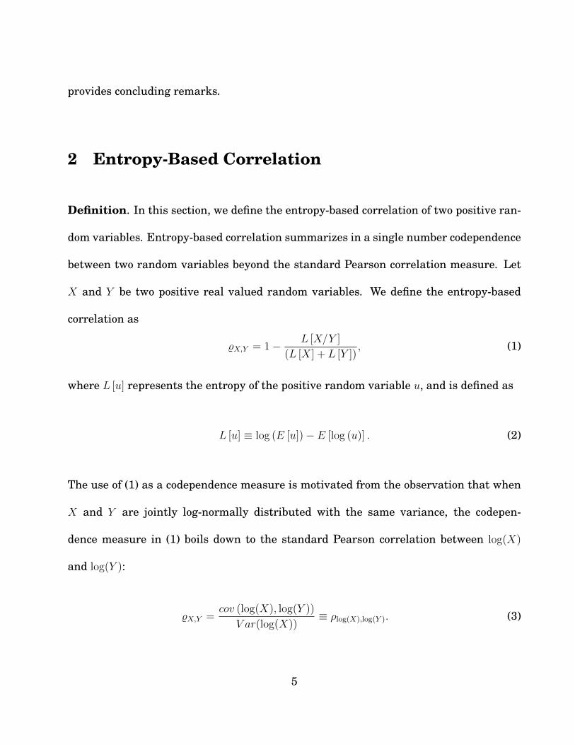
2 Entropy-Based Correlation

Definition. In this section, we define the entropy-based correlation of two positive ran-

dom variables. Entropy-based correlation summarizes in a single number codependence

between two random variables beyond the standard Pearson correlation measure. Let

X and Y be two positive real valued random variables. We define the entropy-based

correlation as

%X,Y = 1− L [X/Y ]

(L [X] + L [Y ]), (1)

where L [u] represents the entropy of the positive random variable u, and is defined as

L [u] ≡ log (E [u])− E [log (u)] . (2)

The use of (1) as a codependence measure is motivated from the observation that when

X and Y are jointly log-normally distributed with the same variance, the codepen-

dence measure in (1) boils down to the standard Pearson correlation between log(X)

and log(Y ):

%X,Y =cov (log(X), log(Y ))

V ar(log(X))≡ ρlog(X),log(Y ). (3)

5

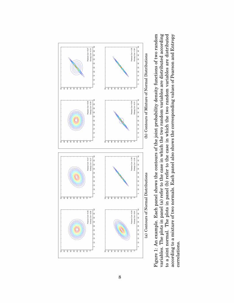
Discussion. We propose an example to document some of the differences between the

proposed entropy-based correlation measure and the standard Pearson correlation mea-

sure. The example proceeds as follows. We shall consider two sets of bivariate distri-

butions. In one case, we focus on joint-normal distributions with a varying degree of

correlation; in the other case, instead, we focus on a mixture of two joint-normal dis-

tributions. The two sets of distributions have two things in common: all the moments

of the marginal distributions are identical, and, most importantly, the Pearson correla-

tions are exactly the same. We shall make the case, however, that the the high-order

codependence terms are very different across the two cases, thus resulting in a different

degree of entropy-correlation.

We shall now describe in greater detail the construction of the two sets of distributions.

In one case, we draw a sample from a bivariate standard normal distribution, in which

the correlation of the random variables is a non negative value that we denote w1. The

four plots in panel (a) of Figure 1 report the contours of the joint probability distribu-

tion associated to four cases for w1. Note that in all four cases the entropy correlation

coincides with the standard measure of correlation.

For the case of the multivariate mixture of normals, we draw a random sample (x1, y1),

(x2, y2), ..., (xn, yn) according to the probability distribution function

p(x, y|µ, S, w) = (1− w1)φ1 (x, y|µ1, S1) + w1φ2 (x, y|µ2, S2)

6

where φ1 (x, y|µ1, S1) and φ1 (x, y|µ1, S1) are normal probability distribution functions

with means µ1 and µ2 and covariance matrices S1 and S2, respectively; w1 and 1 − w1

are non-negative weights attached to them.

For simplicity, we shall assume that µ1 = µ2 = [0, 0]′ and that

S1 =

1 0

0 1

, S2 =

1 1

1 1

Similarly, we are going to draw a sample from a mixture of two normals: one in which x

and y are uncorrelated and one in which x and y are perfectly correlated.

Panel (a) of Figure 1 reports the contours of the joint-normal probability distribution.

Note that in all four plots, the Pearson correlation is exactly identical to the correspond-

ing plots in panel (b). Judging by the moments of the marginal distributions and by the

degree of Pearson correlations, we would not be able to distinguish the distributions in

the two sets of plots.

In panel (b), however, there is a very different extent of non linear codependence between

the two random variables. Specifically, it seems to be the case that the extent of codepen-

dence in the tails of the distribution is lower in the case of the mixture of normals. This

difference is being captured by the entropy-based correlation, which is always below the

standard measure of correlation. In the same manner, the entropy-based correlation

captures high order codependence terms, whereas the Pearson correlation appears to be

7

510

1520

2530

3540

4550

5101520253035404550

510

1520

2530

3540

4550

5101520253035404550

510

1520

2530

3540

4550

5101520253035404550

510

1520

2530

3540

4550

5101520253035404550

Pea

rson

Cor

r =

0.00

Ent

ropy

Cor

r =

0.00

Pea

rson

Cor

r =

0.27

Ent

ropy

Cor

r =

0.27

Pea

rson

Cor

r =

0.64

Ent

ropy

Cor

r =

0.64

Pea

rson

Cor

r =

1.00

Ent

ropy

Cor

r =

1.00

(a)

Con

tour

sof

Nor

mal

Dis

trib

utio

ns

510

1520

2530

3540

4550

5101520253035404550

510

1520

2530

3540

4550

5101520253035404550

510

1520

2530

3540

4550

5101520253035404550

510

1520

2530

3540

4550

5101520253035404550

Pea

rson

Cor

r =0.

00

Ent

ropy

Cor

r =0.

00

Pea

rson

Cor

r =0.

27

Ent

ropy

Cor

r =0.

19

Pea

rson

Cor

r =0.

64

Ent

ropy

Cor

r =0.

51

Pea

rson

Cor

r =1.

00

Ent

ropy

Cor

r =1.

00

(b)

Con

tour

sof

Mix

ture

ofN

orm

alD

istr

ibut

ions

Fig

ure

1:A

nex

ampl

e.E

ach

pane

lsho

ws

the

cont

ours

ofth

ejo

int

prob

abili

tyde

nsit

yfu

ncti

ons

oftw

ora

ndom

vari

able

s.T

hepl

ots

inpa

nel(

a)re

fer

toth

eca

sein

whi

chth

etw

ora

ndom

vari

able

sar

edi

stri

bute

dac

cord

ing

toa

join

tno

rmal

.T

hepl

ots

inpa

nel

(b)

refe

rto

the

case

inw

hich

the

two

rand

omva

riab

les

are

dist

ribu

ted

acco

rdin

gto

am

ixtu

reof

two

norm

als.

Eac

hpa

nela

lso

show

sth

eco

rres

pond

ing

valu

esof

Pear

son

and

Ent

ropy

corr

elat

ions

.

8

insensitive to it.

This observation is relevant for our analysis because it suggests that our entropy-based

correlation is a more comprehensive measure of codependence, one that seems to be

robust to non-normalities, a common feature of SDF’s in the cross-section of countries.

3 Asset Pricing Restrictions on One-Period Co-Entropies

3.1 Stochastic Discount Factors

Preliminaries and Notation. We start by considering two countries, domestic and for-

eign, with SDFs M and M∗, respectively. To ease notations, we drop the time subscript

from the SDF notation. Lowercase letters indicate logarithms of uppercase letters. We

denote by m = log (M) and m∗ = log (M∗). We then consider the sets of SDFs that cor-

rectly price the risk-free bond, the return on the long-term bond, and a generic set of

risky assets

S ≡{M > 0 : E [M ] = 1/Rf , E [MR∞] = 1 and E [MR] = 1

},

S∗ ≡{M∗ > 0 : E [M∗] = 1/R∗f , E [M∗R∗∞] = 1 and E [M∗R∗] = 1

}.

R and R∗ are the set of risky asset returns for both domestic and foreign countries. R∗∞

and R∞ are the gross returns on the long-term bond in both countries. If we further

9

assume that markets are complete, then the growth rate between the currencies of the

two countries is uniquely identified as the the ratio of the stochastic discount factors:

exp(∆e) = M∗/M .

The dispersion in the growth rate of the exchange rate can be decomposed into the sum

of foreign and individual SDF entropies, as well as codependence between the foreign

and domestic SDFs

L [exp (∆e)] = L

[M∗

M

]− (L [M∗] + L [M ])︸ ︷︷ ︸

co-entropy between M∗ and M

+ (L [M∗] + L [M ])︸ ︷︷ ︸sum of individual entropies

. (4)

Expression (4) clearly shows that there are two sources of dispersion in the growth rate

of exchange rates. First, dispersion in the growth rate of exchange rates can be at-

tributed to dispersion in individual entropies. Second, dispersion in the growth rate of

exchange rates can be attributed to the entropy-based correlation of M∗ and M . Di-

viding both the left and right hand sides of (4) by the sum of individual entropies and

rearranging terms yields the entropy-based codependence between foreign and domestic

SDFs:

%M∗,M = 1− L [exp (∆e)]

(L [M∗] + L [M ]), (5)

10

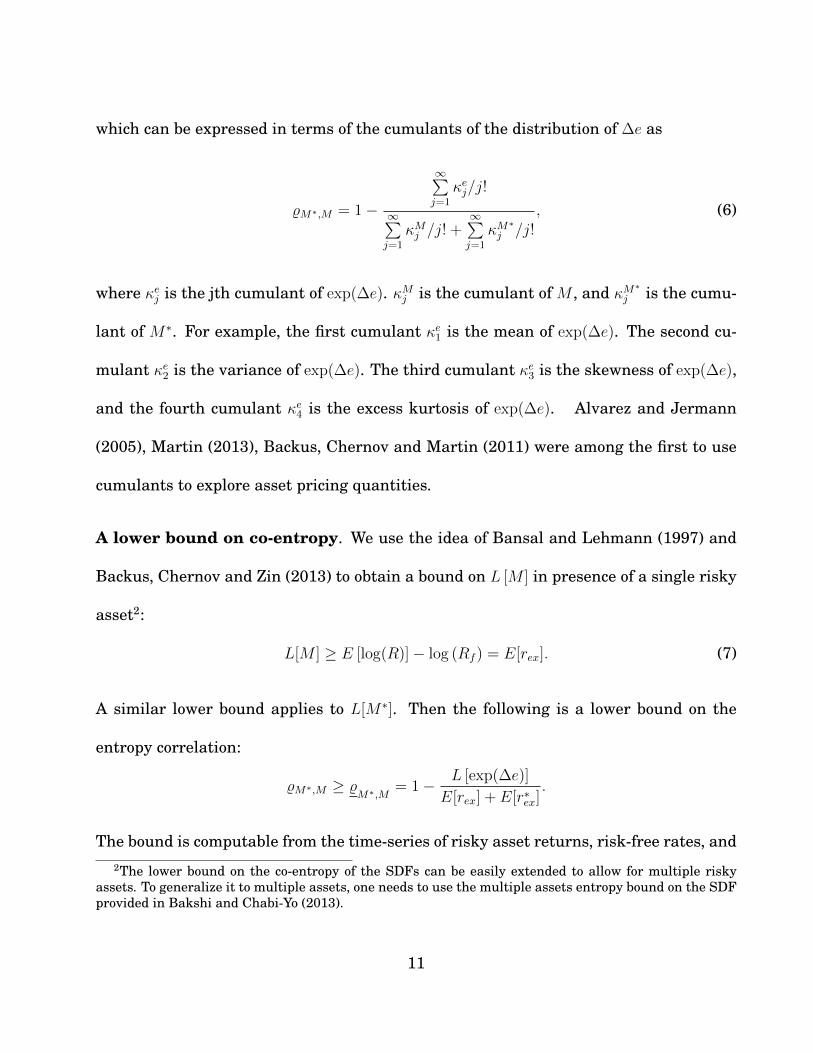
which can be expressed in terms of the cumulants of the distribution of ∆e as

%M∗,M = 1−

∞∑j=1

κej/j!

∞∑j=1

κMj /j! +∞∑j=1

κM∗

j /j!, (6)

where κej is the jth cumulant of exp(∆e). κMj is the cumulant of M , and κM∗j is the cumu-

lant of M∗. For example, the first cumulant κe1 is the mean of exp(∆e). The second cu-

mulant κe2 is the variance of exp(∆e). The third cumulant κe3 is the skewness of exp(∆e),

and the fourth cumulant κe4 is the excess kurtosis of exp(∆e). Alvarez and Jermann

(2005), Martin (2013), Backus, Chernov and Martin (2011) were among the first to use

cumulants to explore asset pricing quantities.

A lower bound on co-entropy. We use the idea of Bansal and Lehmann (1997) and

Backus, Chernov and Zin (2013) to obtain a bound on L [M ] in presence of a single risky

asset2:

L[M ] ≥ E [log(R)]− log (Rf ) = E[rex]. (7)

A similar lower bound applies to L[M∗]. Then the following is a lower bound on the

entropy correlation:

%M∗,M ≥ %M∗,M

= 1− L [exp(∆e)]

E[rex] + E[r∗ex].

The bound is computable from the time-series of risky asset returns, risk-free rates, and2The lower bound on the co-entropy of the SDFs can be easily extended to allow for multiple risky

assets. To generalize it to multiple assets, one needs to use the multiple assets entropy bound on the SDFprovided in Bakshi and Chabi-Yo (2013).

11

exchange rates.

3.2 Decomposing the Entropy-based Correlation

Motivated by recent works in Alvarez and Jermann (2005), Hansen, Heaton and Li

(2008), Hansen and Scheinkman (2009), and Hansen (2012), we postulate that any SDF

M ∈ S, and M∗ ∈ S∗ can be decomposed into permanent and transitory components

M∗ = M∗PM∗T with E[M∗P ] = 1 and M∗T = 1/R∗∞,

M = MPMT with E[MP

]= 1 and MT = 1/R∞.

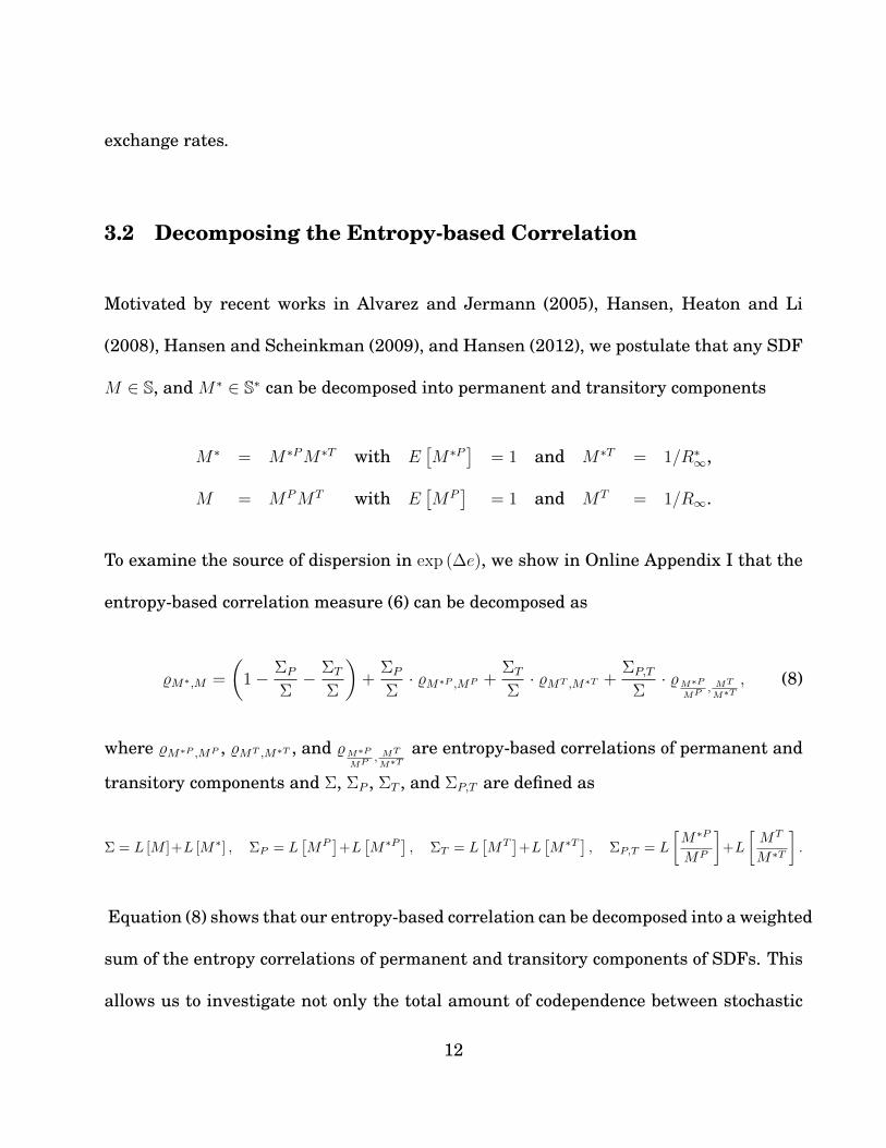
To examine the source of dispersion in exp (∆e), we show in Online Appendix I that the

entropy-based correlation measure (6) can be decomposed as

%M∗,M =

(1− ΣP

Σ− ΣT

Σ

)+

ΣP

Σ· %M∗P ,MP +

ΣT

Σ· %MT ,M∗T +

ΣP,T

Σ· %M∗P

MP , MT

M∗T, (8)

where %M∗P ,MP , %MT ,M∗T , and %M∗PMP , MT

M∗Tare entropy-based correlations of permanent and

transitory components and Σ, ΣP , ΣT , and ΣP,T are defined as

Σ = L [M ]+L [M∗] , ΣP = L[MP

]+L

[M∗P ] , ΣT = L

[MT

]+L

[M∗T ] , ΣP,T = L

[M∗P

MP

]+L

[MT

M∗T

].

Equation (8) shows that our entropy-based correlation can be decomposed into a weighted

sum of the entropy correlations of permanent and transitory components of SDFs. This

allows us to investigate not only the total amount of codependence between stochastic

12

discount factors but also the source of such codependence.

More specifically, codependence between SDFs can be attributed to codependence in per-

manent components of SDFs, codependence in transitory components of SDFs, or code-

pendence of the ratios of permanent components and the ratio of transitory components

of SDFs. In what follows, we provide new restrictions on the additional codependence

terms reported in equation (8).

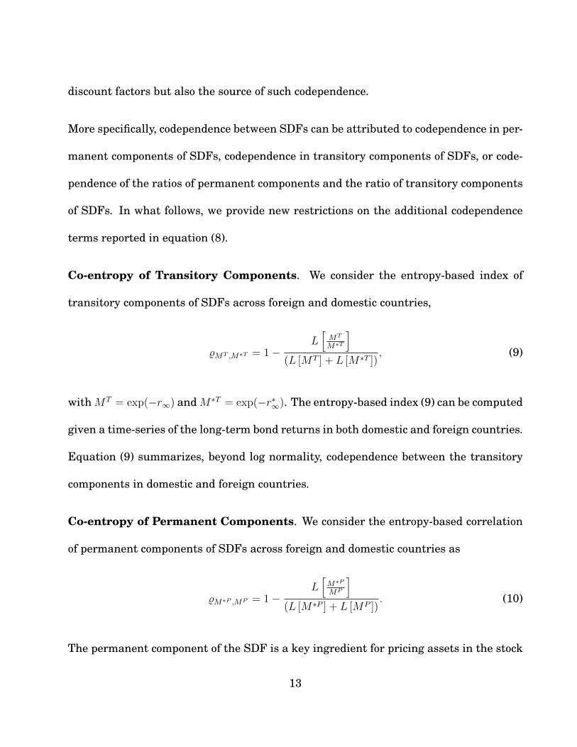
Co-entropy of Transitory Components. We consider the entropy-based index of

transitory components of SDFs across foreign and domestic countries,

%MT ,M∗T = 1−L[MT

M∗T

](L [MT ] + L [M∗T ])

, (9)

withMT = exp(−r∞) andM∗T = exp(−r∗∞). The entropy-based index (9) can be computed

given a time-series of the long-term bond returns in both domestic and foreign countries.

Equation (9) summarizes, beyond log normality, codependence between the transitory

components in domestic and foreign countries.

Co-entropy of Permanent Components. We consider the entropy-based correlation

of permanent components of SDFs across foreign and domestic countries as

%M∗P ,MP = 1−L[M∗P

MP

](L [M∗P ] + L [MP ])

. (10)

The permanent component of the SDF is a key ingredient for pricing assets in the stock

13

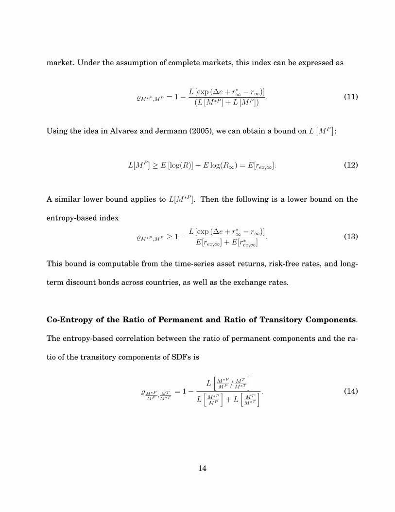
market. Under the assumption of complete markets, this index can be expressed as

%M∗P ,MP = 1− L [exp (∆e+ r∗∞ − r∞)]

(L [M∗P ] + L [MP ]). (11)

Using the idea in Alvarez and Jermann (2005), we can obtain a bound on L[MP

]:

L[MP ] ≥ E [log(R)]− E log(R∞) = E[rex,∞]. (12)

A similar lower bound applies to L[M∗P ]. Then the following is a lower bound on the

entropy-based index

%M∗P ,MP ≥ 1− L [exp (∆e+ r∗∞ − r∞)]

E[rex,∞] + E[r∗ex,∞]. (13)

This bound is computable from the time-series asset returns, risk-free rates, and long-

term discount bonds across countries, as well as the exchange rates.

Co-Entropy of the Ratio of Permanent and Ratio of Transitory Components.

The entropy-based correlation between the ratio of permanent components and the ra-

tio of the transitory components of SDFs is

%M∗PMP , MT

M∗T= 1−

L[M∗P

MP /MT

M∗T

]L[M∗P

MP

]+ L

[MT

M∗T

] . (14)

14

Using an argument similar to the earlier sections, it can be shown that

%M∗PMP , MT

M∗T= 1− L [exp (∆e)]

L [exp (∆e+ r∗∞ − r∞)] + L [exp (r∗∞ − r∞)]. (15)

This expression can be recovered from a time-series of long-term bond returns and ex-

change rates. If M∗P

MP and MT

M∗Tare highly dependent, (14) will be close to 1.

4 Dynamics in Entropy-Based Correlation

Preliminaries and Notation. In this section, we propose measures to capture dy-

namics in the entropy-based index. Hansen (2013), Borovicka and Hansen (2013), and

Backus et al. (2013) emphasize the importance of evaluating asset pricing models over

alternative horizons. Specifically, we are interested in the impact of compounding SDFs,

compounding permanent (transitory) components of SDFs over alternative investment

horizons on entropy-based correlation.

We consider the sets of SDFs that correctly price the risk-free asset, the long-term dis-

count bound, and a set of risky assets:

Sn ={Mt,t+n > 0 : E [Mt,t+n] = Mn, E [Mt,t+nR∞,t,t+n] = 1 and E [Mt,t+nRt,t+n] = 1

},

S∗n ={M∗

t,t+n > 0 : E[M∗

t,t+n

]= M

∗n, E

[M∗

t,t+nR∗∞,t,t+n

]= 1 and E

[M∗

t,t+nR∗t,t+n

]= 1

},

15

where R∞,t,t+n and R∗∞,t,t+n are returns on long-term discount bonds when bonds are

held from t to t + n. Rt,t+n and R∗t,t+n are the set of n-period risky asset returns. Under

no arbitrage conditions, the growth rate between currencies of two countries, when the

investment horizon is n, is given by

exp (∆et,t+n) =M∗

t,t+n

Mt,t+n

,

and the SDFs can be decomposed as a product of one-period SDFs (compounding SDFs):

M∗t,t+n =

n∏i=1

M∗t+i−1,t+i and Mt,t+n =

n∏i=1

Mt+i−1,t+i,

where M∗t+i−1,t+i and Mt+i−1,t+i represent the foreign and domestic stochastic discount

factors over the time interval [t+ i− 1, t+ i]. Similar to Section 3.2, we postulate that

SDFs can be decomposed into permanent and transitory components:

M∗t+i−1,t+i = M∗P

t+i−1,t+iM∗Tt+i−1,t+i,

Mt+i−1,t+i = MPt+i−1,t+iM

Tt+i−1,t+i,

where

M∗Tt+i−1,t+i = 1/R∗∞,t+i−1,t+i and MT

t+i−1,t+i = 1/R∞,t+i−1,t+i.

R∗∞,t+i−1,t+i and R∞,t+i−1,t+i are the returns on the long-term bond in foreign and domestic

countries. In sections to follow, the lowercase letters are a log of the uppercase letters.

16

For example, r∞,t+i−1,t+i = log (R∞,t+i−1,t+i).

Multiperiod Co-Entropy of SDFs. We apply the co-entropy operator to the multi-

period stochastic discount factors defined in equation (4) and obtain:

%Mt,t+n,M∗t,t+n= 1−

L[M∗t,t+n

Mt,t+n

](L [Mt,t+n] + L

[M∗

t,t+n

]) .We shall define the n-periods horizon codependence of the entropy-based correlation as

the difference between the co-entropies of the n-periods and the one-period stochastic

discount factors:

H [n] = %Mt,t+n,M∗t,t+n− %Mt,t+1,M∗t,t+1

. (16)

Co-Entropy of Permanent and Transitory Components. The decomposition of the

entropy-based correlation reported in the equation in Section 3.2 also applies to the

n-periods stochastic discount factors, after defining the n-periods multi-period entropy

indices of permanent and transitory components as

%M it,t+n,M

i∗t,t+n

= 1−L[M∗it,t+n

M it,t+n

](L[M i

t,t+n

]+ L

[M∗i

t,t+n

]) , ∀i ∈ {P, T} (17)

%M∗Pt,t+n

MPt,t+n

,MT

t,t+n

M∗Tt,t+n

= 1−L[M∗Pt,t+n

MPt,t+n

/MT

t,t+n

M∗Tt,t+n

]L[M∗Pt,t+n

MPt,t+n

]+ L

[MT

t,t+n

M∗Tt,t+n

] .The definition of horizon codependence also applies to the entropy-based correlations

17

in (17), and we denote them as HP [n], HT [n], and HPT [n]:

HP [n] = %MPt,t+n,M

∗Pt,t+n− %MP

t,t+1,M∗Pt,t+1

, (18)

HT [n] = %M∗Tt,t+n,MTt,t+n− %M∗Tt,t+1,M

Tt,t+1

, (19)

HPT [n] = %M∗Pt,t+n

MPt,t+n

,MT

t,t+n

M∗Tt,t+n

− %M∗Pt,t+1

MPt,t+1

,MT

t,t+1

M∗Tt,t+1

. (20)

The lower bound on the co-entropy index of the permanent components of the one-period

stochastic discount factors in equation (13) generalizes to the permanent components of

the n-periods stochastic discount factor. We omit the formula of the lower bound in the

interest of space.

Additionally, we show in Online Appendix II that the following upper bound applies to

the horizon codependence of the permanent components of SDFs:

HP [n] ≤L[exp

(∆et,t+1 + r∗t,t+1,∞ − rt,t+1,∞

)]− 1

nL[exp

(∆et,t+n + r∗t,t+n,∞ − rt,t+n,∞

)]E [rt,t+1,ex,∞] + E

[r∗t,t+1,ex,∞

] ,

(21)

with E[rt,t+1,ex,∞] = E [rt,t+1 − r∞,t,t+1] and E[r∗t,t+1,ex,∞] = E[r∗t,t+1 − r∗∞,t,t+1

]. While one

may expect the entropy-based correlation of permanent components of SDFs to exhibit

dynamics when the investor horizon increases, (21) suggests that we should not expect

“too much” dynamics in this co-entropy measure. The maximum amount of dynamics

can be estimated from asset prices without making any modeling assumptions about the

permanent and transitory components of SDFs.

18

5 Empirical Analysis

Description of the data. We collected monthly data on stock market returns, risk-

free rates, ten-year bond yields, CPI inflation, and exchange rates versus US dollars for

16 countries, in addition to the United States. For Belgium, Canada, France, Germany,

Italy, Japan, Spain, Switzerland, United Kingdom, and United States, the sample starts

in January 1975 and ends in May 2013. For Austria, the sample starts in June 1989,

for Denmark and Finland in January 1987, for Ireland in February 1995, for Denmark

in January 1986, Norway in January 1979, and for Sweden in January 1982. Real

variables are constructed by dividing nominal variables by realized CPI inflation.

Stock market returns for all countries are value-weighted returns in local currency col-

lected from Kenneth French’s website.3 Risk-free rates are collected as the three-month

interest rates on Government Bills. The data source is the International Monetary

Fund (International Financial Statistics) for Canada, France, Germany, Italy, Japan,

the Netherlands, Spain, the UK, and the US ; for the following countries data are in-

stead collected from the OECD: Austria, Belgium, Denmark, Finland, Ireland, Norway,

Sweden, and Switzerland.

Long-term rates are collected as the ten-year interest rates on government bonds. The

data source is the International Monetary Fund (International Financial Statistics) for3This dataset is publicly available at http://mba.tuck.dartmouth.edu/pages/faculty/ken.

french/data_library.html#International.

19

all countries. CPI inflation is computed as the growth rate of the “Total Items” index in

two consecutive months. The data source is OECD for all countries. Exchange rates are

collected in units of foreign currency per US dollar. The source is the Federal Reserve

of St. Louis for all countries, with the exception of Canada, Denmark, Japan, Norway,

Sweden, Switzerland, and the United Kingdom, for which the source is the Federal

Reserve Board.

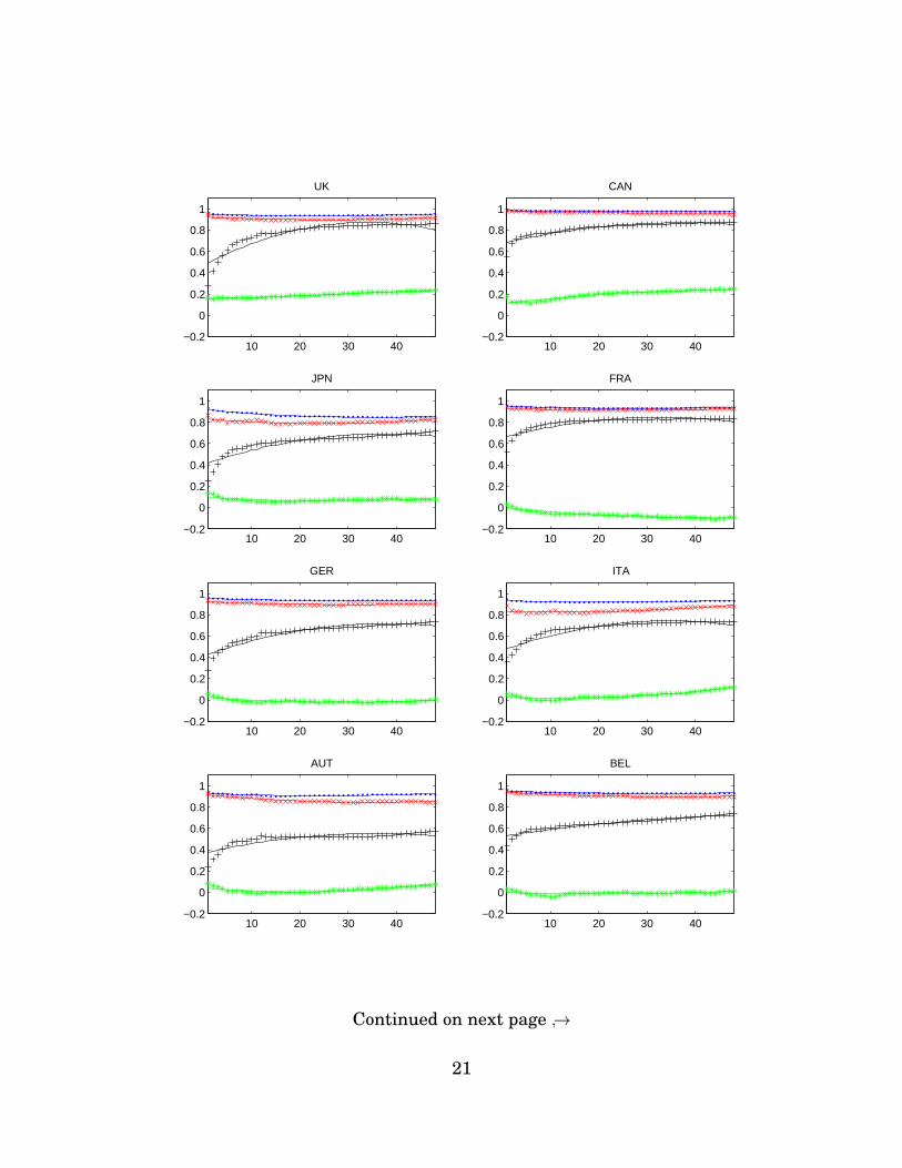
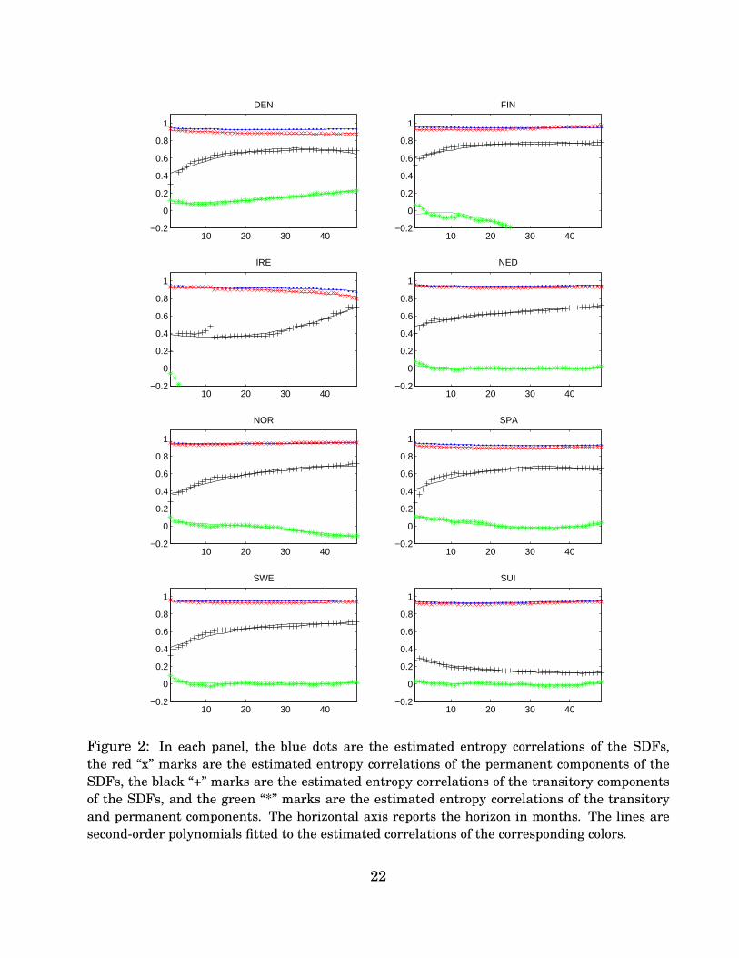
Co-entropies in the cross-section of countries. Figure 2 reports the estimated

entropy correlations for the 16 countries in our sample. The United States is always

assumed to be the home country. Specifically, for each country pair, we report the es-

timated entropy correlations for horizons ranging between 1 and 48 months. A few

consistent findings appear to emerge from this analysis.

The lower bounds on the entropy correlations of the total SDFs (black dots in each panel)

are always extremely large. This confirms the findings of Brandt et al. (2006) that

SDFs ought to be very correlated across countries to explain the degree of dispersion of

exchange rate fluctuations.

Our analysis allows us to dig deeper into the components responsible for such a high

degree of codependence of the SDFs. The co-entropy of the permanent components (red

crosses) are also very close to 1 across all panels, suggesting that an overwhelming

majority of the comovement of SDFs is accounted for by these components.

The entropy-based correlations of the transitory components (black pluses) display the

20

10 20 30 40−0.2

0

0.2

0.4

0.6

0.8

1

UK

10 20 30 40−0.2

0

0.2

0.4

0.6

0.8

1

CAN

10 20 30 40−0.2

0

0.2

0.4

0.6

0.8

1

JPN

10 20 30 40−0.2

0

0.2

0.4

0.6

0.8

1

FRA

10 20 30 40−0.2

0

0.2

0.4

0.6

0.8

1

GER

10 20 30 40−0.2

0

0.2

0.4

0.6

0.8

1

ITA

10 20 30 40−0.2

0

0.2

0.4

0.6

0.8

1

AUT

10 20 30 40−0.2

0

0.2

0.4

0.6

0.8

1

BEL

Continued on next page ↪→

21

10 20 30 40−0.2

0

0.2

0.4

0.6

0.8

1

DEN

10 20 30 40−0.2

0

0.2

0.4

0.6

0.8

1

FIN

10 20 30 40−0.2

0

0.2

0.4

0.6

0.8

1

IRE

10 20 30 40−0.2

0

0.2

0.4

0.6

0.8

1

NED

10 20 30 40−0.2

0

0.2

0.4

0.6

0.8

1

NOR

10 20 30 40−0.2

0

0.2

0.4

0.6

0.8

1

SPA

10 20 30 40−0.2

0

0.2

0.4

0.6

0.8

1

SWE

10 20 30 40−0.2

0

0.2

0.4

0.6

0.8

1

SUI

Figure 2: In each panel, the blue dots are the estimated entropy correlations of the SDFs,the red “x” marks are the estimated entropy correlations of the permanent components of theSDFs, the black “+” marks are the estimated entropy correlations of the transitory componentsof the SDFs, and the green “*” marks are the estimated entropy correlations of the transitoryand permanent components. The horizontal axis reports the horizon in months. The lines aresecond-order polynomials fitted to the estimated correlations of the corresponding colors.

22

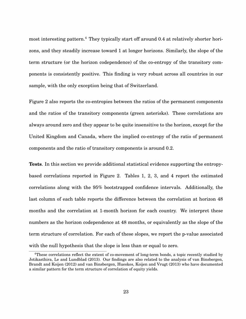
most interesting pattern.4 They typically start off around 0.4 at relatively shorter hori-

zons, and they steadily increase toward 1 at longer horizons. Similarly, the slope of the

term structure (or the horizon codependence) of the co-entropy of the transitory com-

ponents is consistently positive. This finding is very robust across all countries in our

sample, with the only exception being that of Switzerland.

Figure 2 also reports the co-entropies between the ratios of the permanent components

and the ratios of the transitory components (green asterisks). These correlations are

always around zero and they appear to be quite insensitive to the horizon, except for the

United Kingdom and Canada, where the implied co-entropy of the ratio of permanent

components and the ratio of transitory components is around 0.2.

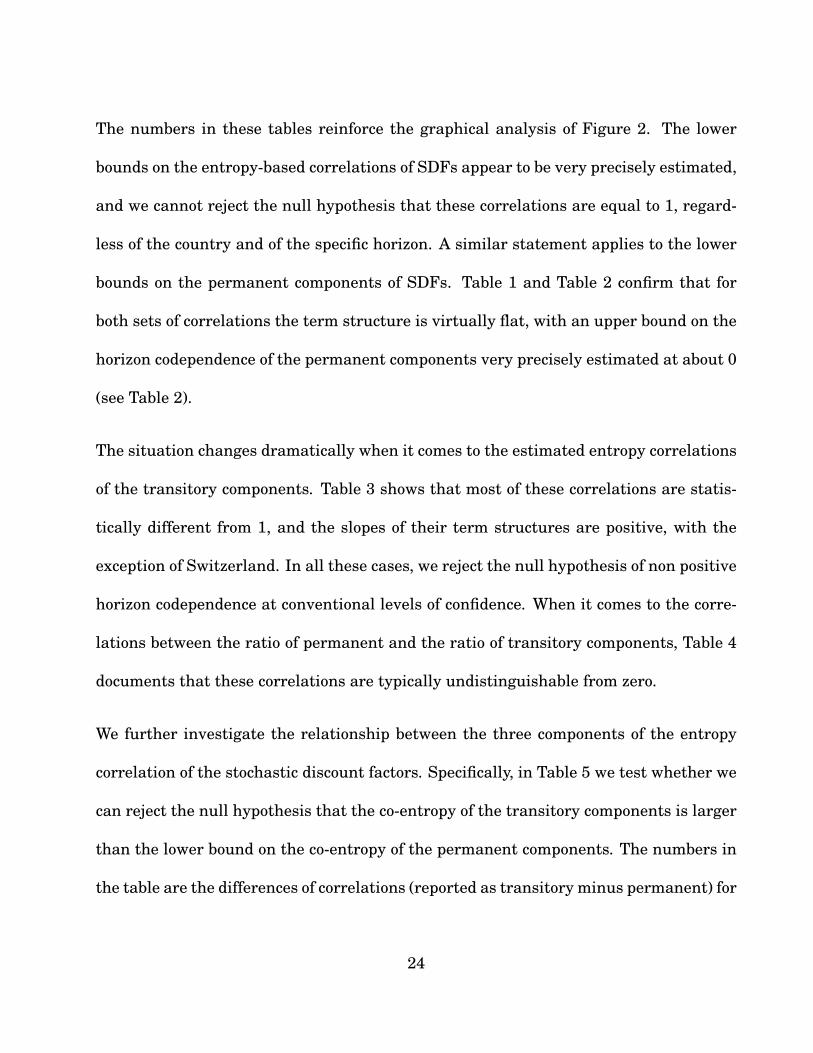
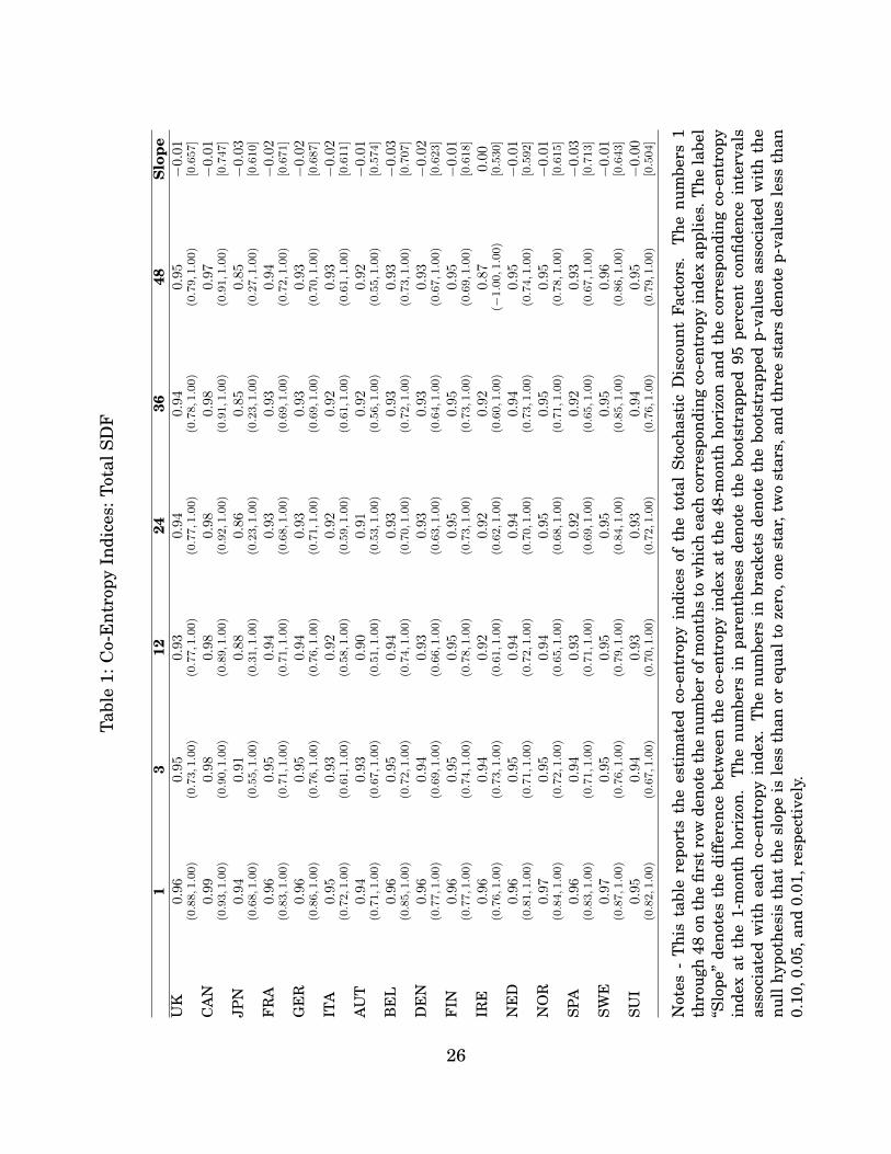
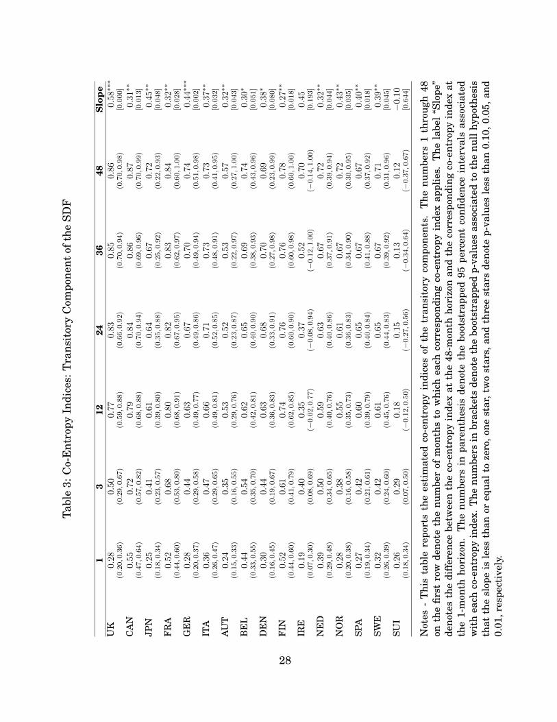
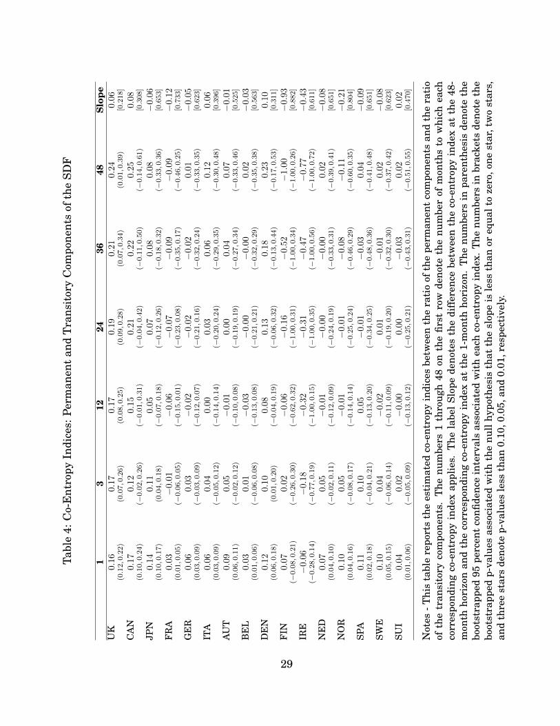
Tests. In this section we provide additional statistical evidence supporting the entropy-

based correlations reported in Figure 2. Tables 1, 2, 3, and 4 report the estimated

correlations along with the 95% bootstrapped confidence intervals. Additionally, the

last column of each table reports the difference between the correlation at horizon 48

months and the correlation at 1-month horizon for each country. We interpret these

numbers as the horizon codependence at 48 months, or equivalently as the slope of the

term structure of correlation. For each of these slopes, we report the p-value associated

with the null hypothesis that the slope is less than or equal to zero.4These correlations reflect the extent of co-movement of long-term bonds, a topic recently studied by

Jotikasthira, Le and Lundblad (2013). Our findings are also related to the analysis of van Binsbergen,Brandt and Koijen (2012) and van Binsbergen, Hueskes, Koijen and Vrugt (2013) who have documenteda similar pattern for the term structure of correlation of equity yields.

23

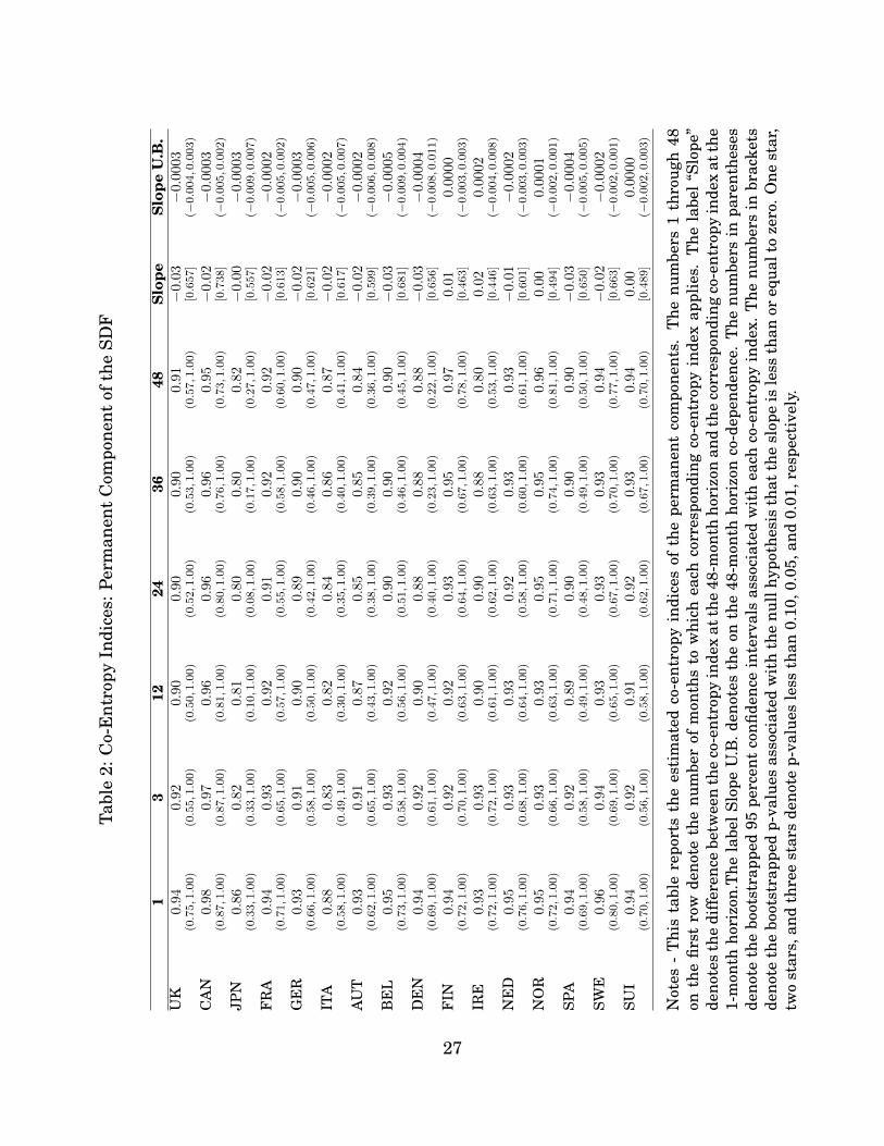
The numbers in these tables reinforce the graphical analysis of Figure 2. The lower

bounds on the entropy-based correlations of SDFs appear to be very precisely estimated,

and we cannot reject the null hypothesis that these correlations are equal to 1, regard-

less of the country and of the specific horizon. A similar statement applies to the lower

bounds on the permanent components of SDFs. Table 1 and Table 2 confirm that for

both sets of correlations the term structure is virtually flat, with an upper bound on the

horizon codependence of the permanent components very precisely estimated at about 0

(see Table 2).

The situation changes dramatically when it comes to the estimated entropy correlations

of the transitory components. Table 3 shows that most of these correlations are statis-

tically different from 1, and the slopes of their term structures are positive, with the

exception of Switzerland. In all these cases, we reject the null hypothesis of non positive

horizon codependence at conventional levels of confidence. When it comes to the corre-

lations between the ratio of permanent and the ratio of transitory components, Table 4

documents that these correlations are typically undistinguishable from zero.

We further investigate the relationship between the three components of the entropy

correlation of the stochastic discount factors. Specifically, in Table 5 we test whether we

can reject the null hypothesis that the co-entropy of the transitory components is larger

than the lower bound on the co-entropy of the permanent components. The numbers in

the table are the differences of correlations (reported as transitory minus permanent) for

24

each horizon and each country pair. The point estimates are all negative, significantly

so for most countries at horizons less than 12 months. For horizons longer than one

year, we can still reject the null for a majority of the cases, although the result appears

to be less and less evident as the horizon increases.

The picture that seems to emerge from this analysis is one in which the correlation

of the transitory components increases over time and is significantly smaller than the

correlation of the permanent components at the very least for horizons up to one year.

These findings are important because they impose very tight restrictions on interna-

tional asset pricing models as far as the dynamics and the ranking of correlations are

concerned.

We conclude this analysis by documenting that the co-entropy between the ratio of per-

manent and the ratio of the transitory components is always significantly smaller than

the lower bound on the correlation of the permanent components. This set of tests is

carried out in Table 6.

25

Tabl

e1:

Co-

Ent

ropy

Indi

ces:

Tota

lSD

F

13

1224

3648

Slop

eU

K0.

960.

950.

93

0.94

0.94

0.9

5−

0.01

(0.88,1.00)

(0.73,1.00)

(0.77,1.00)

(0.77,1.00)

(0.78,1.00)

(0.79,1.00)

[0.657]

CA

N0.

990.

980.

98

0.98

0.98

0.9

7−

0.01

(0.93,1.00)

(0.90,1.00)

(0.89,1.00)

(0.92,1.00)

(0.91,1.00)

(0.91,1.00)

[0.747]

JPN

0.94

0.91

0.88

0.86

0.85

0.8

5−

0.03

(0.68,1.00)

(0.55,1.00)

(0.31,1.00)

(0.23,1.00)

(0.23,1.00)

(0.27,1.00)

[0.610]

FR

A0.

960.

950.

94

0.93

0.93

0.9

4−

0.02

(0.83,1.00)

(0.71,1.00)

(0.71,1.00)

(0.68,1.00)

(0.69,1.00)

(0.72,1.00)

[0.671]

GE

R0.

960.

950.

94

0.93

0.93

0.9

3−

0.02

(0.86,1.00)

(0.76,1.00)

(0.76,1.00)

(0.71,1.00)

(0.69,1.00)

(0.70,1.00)

[0.687]

ITA

0.9

50.

930.

92

0.92

0.92

0.9

3−

0.02

(0.72,1.00)

(0.61,1.00)

(0.58,1.00)

(0.59,1.00)

(0.61,1.00)

(0.61,1.00)

[0.611]

AU

T0.9

40.

930.

90

0.91

0.92

0.9

2−

0.0

1(0.71,1.00)

(0.67,1.00)

(0.51,1.00)

(0.53,1.00)

(0.56,1.00)

(0.55,1.00)

[0.574]

BE

L0.9

60.

950.

94

0.93

0.93

0.9

3−

0.0

3(0.85,1.00)

(0.72,1.00)

(0.74,1.00)

(0.70,1.00)

(0.72,1.00)

(0.73,1.00)

[0.707]

DE

N0.9

60.

940.

93

0.93

0.93

0.9

3−

0.0

2(0.77,1.00)

(0.69,1.00)

(0.66,1.00)

(0.63,1.00)

(0.64,1.00)

(0.67,1.00)

[0.623]

FIN

0.96

0.95

0.95

0.95

0.95

0.9

5−

0.0

1(0.77,1.00)

(0.74,1.00)

(0.78,1.00)

(0.73,1.00)

(0.73,1.00)

(0.69,1.00)

[0.618]

IRE

0.96

0.94

0.92

0.92

0.92

0.8

70.0

0(0.76,1.00)

(0.73,1.00)

(0.61,1.00)

(0.62,1.00)

(0.60,1.00)

(−1.00,1.00)

[0.530]

NE

D0.

960.

950.

94

0.94

0.94

0.9

5−

0.01

(0.81,1.00)

(0.71,1.00)

(0.72,1.00)

(0.70,1.00)

(0.73,1.00)

(0.74,1.00)

[0.592]

NO

R0.

970.

950.

94

0.95

0.95

0.9

5−

0.01

(0.84,1.00)

(0.72,1.00)

(0.65,1.00)

(0.68,1.00)

(0.71,1.00)

(0.78,1.00)

[0.615]

SPA

0.96

0.94

0.93

0.92

0.92

0.9

3−

0.03

(0.83,1.00)

(0.71,1.00)

(0.71,1.00)

(0.69,1.00)

(0.65,1.00)

(0.67,1.00)

[0.713]

SWE

0.97

0.95

0.95

0.95

0.95

0.9

6−

0.01

(0.87,1.00)

(0.76,1.00)

(0.79,1.00)

(0.84,1.00)

(0.85,1.00)

(0.86,1.00)

[0.643]

SUI

0.9

50.

940.

93

0.93

0.94

0.9

5−

0.00

(0.82,1.00)

(0.67,1.00)

(0.70,1.00)

(0.72,1.00)

(0.76,1.00)

(0.79,1.00)

[0.504]

Not

es-

Thi

sta

ble

repo

rts

the

esti

mat

edco

-ent

ropy

indi

ces

ofth

eto

tal

Stoc

hast

icD

isco

unt

Fact

ors.

The

num

bers

1th

roug

h48

onth

efir

stro

wde

note

the

num

ber

ofm

onth

sto

whi

chea

chco

rres

pond

ing

co-e

ntro

pyin

dex

appl

ies.

The

labe

l“S

lope

”de

note

sth

edi

ffer

ence

betw

een

the

co-e

ntro

pyin

dex

atth

e48

-mon

thho

rizo

nan

dth

eco

rres

pond

ing

co-e

ntro

pyin

dex

atth

e1-

mon

thho

rizo

n.T

henu

mbe

rsin

pare

nthe

ses

deno

teth

ebo

otst

rapp

ed95

perc

ent

confi

denc

ein

terv

als

asso

ciat

edw

ith

each

co-e

ntro

pyin

dex.

The

num

bers

inbr

acke

tsde

note

the

boot

stra

pped

p-va

lues

asso

ciat

edw

ith

the

null

hypo

thes

isth

atth

esl

ope

isle

ssth

anor

equa

lto

zero

,one

star

,tw

ost

ars,

and

thre

est

ars

deno

tep-

valu

esle

ssth

an0.

10,0

.05,

and

0.01

,res

pect

ivel

y.

26

Tabl

e2:

Co-

Ent

ropy

Indi

ces:

Perm

anen

tC

ompo

nent

ofth

eSD

F

13

1224

3648

Slop

eSl

ope

U.B

.U

K0.

940.9

20.9

00.9

00.9

00.9

1−

0.03

−0.

0003

(0.75,1.00)

(0.55,1.00)

(0.50,1.00)

(0.52,1.00)

(0.53,1.00)

(0.57,1.00)

[0.657]

(−0.004,0.003)

CA

N0.

980.9

70.9

60.9

60.9

60.9

5−

0.02

−0.

0003

(0.87,1.00)

(0.87,1.00)

(0.81,1.00)

(0.80,1.00)

(0.76,1.00)

(0.73,1.00)

[0.738]

(−0.005,0.002)

JPN

0.86

0.8

20.8

10.8

00.8

00.8

2−

0.00

−0.0

003

(0.33,1.00)

(0.33,1.00)

(0.10,1.00)

(0.08,1.00)

(0.17,1.00)

(0.27,1.00)

[0.557]

(−0.009,0.007)

FR

A0.9

40.9

30.9

20.9

10.9

20.9

2−

0.0

2−

0.0002

(0.71,1.00)

(0.65,1.00)

(0.57,1.00)

(0.55,1.00)

(0.58,1.00)

(0.60,1.00)

[0.613]

(−0.005,0.002)

GE

R0.9

30.9

10.9

00.8

90.9

00.9

0−

0.0

2−

0.0003

(0.66,1.00)

(0.58,1.00)

(0.50,1.00)

(0.42,1.00)

(0.46,1.00)

(0.47,1.00)

[0.621]

(−0.005,0.006)

ITA

0.88

0.8

30.8

20.8

40.8

60.8

7−

0.02

−0.

0002

(0.58,1.00)

(0.49,1.00)

(0.30,1.00)

(0.35,1.00)

(0.40,1.00)

(0.41,1.00)

[0.617]

(−0.005,0.007)

AU

T0.

930.9

10.8

70.8

50.8

50.8

4−

0.02

−0.

0002

(0.62,1.00)

(0.65,1.00)

(0.43,1.00)

(0.38,1.00)

(0.39,1.00)

(0.36,1.00)

[0.599]

(−0.006,0.008)

BE

L0.

950.9

30.9

20.9

00.9

00.9

0−

0.03

−0.

0005

(0.73,1.00)

(0.58,1.00)

(0.56,1.00)

(0.51,1.00)

(0.46,1.00)

(0.45,1.00)

[0.681]

(−0.009,0.004)

DE

N0.

940.9

20.9

00.8

80.8

80.8

8−

0.03

−0.0

004

(0.69,1.00)

(0.61,1.00)

(0.47,1.00)

(0.40,1.00)

(0.23,1.00)

(0.22,1.00)

[0.656]

(−0.008,0.011)

FIN

0.9

40.9

20.9

20.9

30.9

50.9

70.0

10.

0000

(0.72,1.00)

(0.70,1.00)

(0.63,1.00)

(0.64,1.00)

(0.67,1.00)

(0.78,1.00)

[0.463]

(−0.003,0.003)

IRE

0.9

30.9

30.9

00.9

00.8

80.8

00.0

20.

0002

(0.72,1.00)

(0.72,1.00)

(0.61,1.00)

(0.62,1.00)

(0.63,1.00)

(0.53,1.00)

[0.446]

(−0.004,0.008)

NE

D0.

950.9

30.9

30.9

20.9

30.9

3−

0.01

−0.

0002

(0.76,1.00)

(0.68,1.00)

(0.64,1.00)

(0.58,1.00)

(0.60,1.00)

(0.61,1.00)

[0.601]

(−0.003,0.003)

NO

R0.

950.9

30.9

30.9

50.9

50.9

60.0

00.

0001

(0.72,1.00)

(0.66,1.00)

(0.63,1.00)

(0.71,1.00)

(0.74,1.00)

(0.81,1.00)

[0.494]

(−0.002,0.001)

SPA

0.94

0.9

20.8

90.9

00.9

00.9

0−

0.03

−0.

0004

(0.69,1.00)

(0.58,1.00)

(0.49,1.00)

(0.48,1.00)

(0.49,1.00)

(0.50,1.00)

[0.650]

(−0.005,0.005)

SWE

0.96

0.9

40.9

30.9

30.9

30.9

4−

0.02

−0.0

002

(0.80,1.00)

(0.69,1.00)

(0.65,1.00)

(0.67,1.00)

(0.70,1.00)

(0.77,1.00)

[0.663]

(−0.002,0.001)

SUI

0.9

40.9

20.9

10.9

20.9

30.9

40.0

00.

0000

(0.70,1.00)

(0.56,1.00)

(0.58,1.00)

(0.62,1.00)

(0.67,1.00)

(0.70,1.00)

[0.489]

(−0.002,0.003)

Not

es-

Thi

sta

ble

repo

rts

the

esti

mat

edco

-ent

ropy

indi

ces

ofth

epe

rman

ent

com

pone

nts.

The

num

bers

1th

roug

h48

onth

efir

stro

wde

note

the

num

ber

ofm

onth

sto

whi

chea

chco

rres

pond

ing

co-e

ntro

pyin

dex

appl

ies.

The

labe

l“S

lope

”de

note

sth

edi

ffer

ence

betw

een

the

co-e

ntro

pyin

dex

atth

e48

-mon

thho

rizo

nan

dth

eco

rres

pond

ing

co-e

ntro

pyin

dex

atth

e1-

mon

thho

rizo

n.T

hela

belS

lope

U.B

.den

otes

the

onth

e48

-mon

thho

rizo

nco

-dep

ende

nce.

The

num

bers

inpa

rent

hese

sde

note

the

boot

stra

pped

95pe

rcen

tco

nfide

nce

inte

rval

sas

soci

ated

wit

hea

chco

-ent

ropy

inde

x.T

henu

mbe

rsin

brac

kets

deno

teth

ebo

otst

rapp

edp-

valu

esas

soci

ated

wit

hth

enu

llhy

poth

esis

that

the

slop

eis

less

than

oreq

ualt

oze

ro.O

nest

ar,

two

star

s,an

dth

ree

star

sde

note

p-va

lues

less

than

0.10

,0.0

5,an

d0.

01,r

espe

ctiv

ely.

27

Tabl

e3:

Co-

Ent

ropy

Indi

ces:

Tra

nsit

ory

Com

pone

ntof

the

SDF

13

1224

3648

Slop

eU

K0.

280.

500.7

70.

83

0.85

0.86

0.5

8∗∗

∗

(0.20,0.36)

(0.29,0.67)

(0.59,0.88)

(0.66,0.92)

(0.70,0.94)

(0.70,0.98)

[0.000]

CA

N0.

550.

720.7

90.

84

0.86

0.87

0.3

1∗∗

(0.47,0.64)

(0.57,0.82)

(0.68,0.88)

(0.70,0.94)

(0.69,0.96)

(0.70,0.99)

[0.013]

JPN

0.2

50.

410.6

10.

64

0.67

0.72

0.4

5∗∗

(0.18,0.34)

(0.23,0.57)

(0.39,0.80)

(0.35,0.88)

(0.25,0.92)

(0.22,0.93)

[0.048]

FR

A0.5

20.

680.8

00.

82

0.83

0.84

0.3

2∗∗

(0.44,0.60)

(0.53,0.80)

(0.68,0.91)

(0.67,0.95)

(0.62,0.97)

(0.60,1.00)

[0.028]

GE

R0.2

80.

440.6

30.

67

0.70

0.74

0.4

4∗∗

∗

(0.20,0.37)

(0.29,0.58)

(0.49,0.77)

(0.49,0.86)

(0.49,0.94)

(0.51,0.98)

[0.002]

ITA

0.3

60.

470.6

60.

71

0.73

0.73

0.3

7∗∗

(0.26,0.47)

(0.29,0.65)

(0.49,0.81)

(0.52,0.85)

(0.48,0.91)

(0.41,0.95)

[0.032]

AU

T0.2

40.

350.5

30.

52

0.53

0.57

0.3

2∗∗

(0.15,0.33)

(0.16,0.55)

(0.29,0.76)

(0.23,0.87)

(0.22,0.97)

(0.27,1.00)

[0.043]

BE

L0.4

40.

540.6

20.

65

0.69

0.74

0.3

0∗

(0.33,0.55)

(0.35,0.70)

(0.42,0.81)

(0.40,0.90)

(0.38,0.93)

(0.43,0.96)

[0.051]

DE

N0.3

00.

440.6

30.

68

0.70

0.69

0.3

8∗

(0.16,0.45)

(0.19,0.67)

(0.36,0.83)

(0.33,0.91)

(0.27,0.98)

(0.23,0.99)

[0.080]

FIN

0.5

20.

610.7

40.

76

0.76

0.78

0.2

7∗∗

(0.44,0.60)

(0.41,0.79)

(0.62,0.85)

(0.60,0.90)

(0.60,0.98)

(0.60,1.00)

[0.018]

IRE

0.1

90.

400.3

50.

37

0.52

0.70

0.4

5(0.07,0.30)

(0.08,0.69)

(−0.02,0.77)

(−0.08,0.94)

(−0.12,1.00)

(−0.14,1.00)

[0.193]

NE

D0.3

90.

500.5

90.

63

0.67

0.72

0.3

2∗∗

(0.29,0.48)

(0.34,0.65)

(0.40,0.76)

(0.40,0.86)

(0.37,0.91)

(0.39,0.94)

[0.044]

NO

R0.2

80.

380.5

50.

61

0.67

0.72

0.4

3∗∗

(0.20,0.38)

(0.16,0.58)

(0.35,0.73)

(0.36,0.83)

(0.34,0.90)

(0.30,0.95)

[0.035]

SPA

0.2

70.

420.6

00.

65

0.67

0.67

0.4

0∗∗

(0.19,0.34)

(0.21,0.61)

(0.39,0.79)

(0.40,0.84)

(0.41,0.88)

(0.37,0.92)

[0.018]

SWE

0.3

20.

420.6

10.

65

0.67

0.71

0.3

9∗∗

(0.26,0.39)

(0.24,0.60)

(0.45,0.76)

(0.44,0.83)

(0.39,0.92)

(0.31,0.96)

[0.045]

SUI

0.2

60.

290.1

80.

15

0.13

0.12

−0.

10

(0.18,0.34)

(0.07,0.50)

(−0.12,0.50)

(−0.27,0.56)

(−0.34,0.64)

(−0.37,0.67)

[0.644]

Not

es-

Thi

sta

ble

repo

rts

the

esti

mat

edco

-ent

ropy

indi

ces

ofth

etr

ansi

tory

com

pone

nts.

The

num

bers

1th

roug

h48

onth

efir

stro

wde

note

the

num

ber

ofm

onth

sto

whi

chea

chco

rres

pond

ing

co-e

ntro

pyin

dex

appl

ies.

The

labe

l“S

lope

”de

note

sth

edi

ffer

ence

betw

een

the

co-e

ntro

pyin

dex

atth

e48

-mon

thho

rizo

nan

dth

eco

rres

pond

ing

co-e

ntro

pyin

dex

atth

e1-

mon

thho

rizo

n.T

henu

mbe

rsin

pare

nthe

sis

deno

teth

ebo

otst

rapp

ed95

perc

ent

confi

denc

ein

terv

als

asso

ciat

edw

ith

each

co-e

ntro

pyin

dex.

The

num

bers

inbr

acke

tsde

note

the

boot

stra

pped

p-va

lues

asso

ciat

edto

the

null

hypo

thes

isth

atth

esl

ope

isle

ssth

anor

equa

lto

zero

,one

star

,tw

ost

ars,

and

thre

est

ars

deno

tep-

valu

esle

ssth

an0.

10,0

.05,

and

0.01

,res

pect

ivel

y.

28

Tabl

e4:

Co-

Ent

ropy

Indi

ces:

Perm

anen

tan

dT

rans

itor

yC

ompo

nent

sof

the

SDF

13

1224

3648

Slop

eU

K0.1

60.

170.

17

0.19

0.21

0.24

0.0

6(0.12,0.22)

(0.07,0.26)

(0.08,0.25)

(0.09,0.28)

(0.07,0.34)

(0.01,0.39)

[0.218]

CA

N0.1

70.

120.

15

0.21

0.22

0.25

0.0

8(0.10,0.24)

(−0.02,0.26)

(−0.01,0.31)

(−0.04,0.42)

(−0.11,0.50)

(−0.14,0.61)

[0.308]

JPN

0.1

40.

110.

05

0.07

0.08

0.08

−0.

06

(0.10,0.17)

(0.04,0.18)

(−0.07,0.18)

(−0.12,0.26)

(−0.18,0.32)

(−0.33,0.36)

[0.653]

FR

A0.

03−

0.01

−0.0

6−

0.07

−0.

09

−0.0

9−

0.12

(0.01,0.05)

(−0.06,0.05)

(−0.15,0.01)

(−0.23,0.08)

(−0.35,0.17)

(−0.46,0.25)

[0.733]

GE

R0.

060.

03−

0.0

2−

0.02

−0.

02

0.01

−0.

05

(0.03,0.09)

(−0.03,0.09)

(−0.12,0.07)

(−0.21,0.16)

(−0.32,0.24)

(−0.33,0.35)

[0.623]

ITA

0.06

0.04

0.00

0.03

0.06

0.12

0.0

6(0.03,0.09)

(−0.05,0.12)

(−0.14,0.14)

(−0.20,0.24)

(−0.29,0.35)

(−0.30,0.48)

[0.396]

AU

T0.

090.

05−

0.01

0.00

0.04

0.07

−0.0

1(0.06,0.11)

(−0.02,0.12)

(−0.10,0.08)

(−0.19,0.19)

(−0.27,0.34)

(−0.33,0.46)

[0.525]

BE

L0.

030.

01−

0.03

−0.0

0−

0.00

0.02

−0.0

3(0.01,0.06)

(−0.06,0.08)

(−0.13,0.08)

(−0.21,0.21)

(−0.32,0.29)

(−0.35,0.38)

[0.563]

DE

N0.1

20.

100.

08

0.13

0.18

0.23

0.1

0(0.06,0.18)

(0.01,0.20)

(−0.04,0.19)

(−0.06,0.32)

(−0.13,0.44)

(−0.17,0.53)

[0.311]

FIN

0.0

70.

02−

0.06

−0.

16

−0.5

2−

1.00

−0.

93

(−0.08,0.21)

(−0.26,0.30)

(−0.62,0.32)

(−1.00,0.31)

(−1.00,0.34)

(−1.00,0.26)

[0.882]

IRE

−0.

06−

0.18

−0.3

2−

0.31

−0.

47

−0.7

7−

0.43

(−0.28,0.14)

(−0.77,0.19)

(−1.00,0.15)

(−1.00,0.35)

(−1.00,0.56)

(−1.00,0.72)

[0.611]

NE

D0.

070.

05−

0.0

1−

0.00

−0.

00

0.02

−0.

08

(0.04,0.10)

(−0.02,0.11)

(−0.12,0.09)

(−0.24,0.19)

(−0.33,0.31)

(−0.39,0.41)

[0.651]

NO

R0.

100.

05−

0.01

−0.0

1−

0.08

−0.

11

−0.2

1(0.04,0.16)

(−0.08,0.17)

(−0.14,0.14)

(−0.25,0.24)

(−0.46,0.29)

(−0.60,0.35)

[0.804]

SPA

0.11

0.10

0.05

−0.0

1−

0.03

0.04

−0.0

9(0.02,0.18)

(−0.04,0.21)

(−0.13,0.20)

(−0.34,0.25)

(−0.48,0.36)

(−0.41,0.48)

[0.651]

SWE

0.1

00.

04−

0.02

0.01

−0.0

10.

02

−0.

08

(0.05,0.15)

(−0.06,0.14)

(−0.11,0.09)

(−0.19,0.20)

(−0.32,0.30)

(−0.37,0.42)

[0.623]

SUI

0.0

40.

02−

0.00

0.00

−0.0

30.

02

0.0

2(0.01,0.06)

(−0.05,0.09)

(−0.13,0.12)

(−0.25,0.21)

(−0.43,0.31)

(−0.51,0.55)

[0.470]

Not

es-T

his

tabl

ere

port

sth

ees

tim

ated

co-e

ntro

pyin

dice

sbe

twee

nth

era

tio

ofth

epe

rman

ent

com

pone

nts

and

the

rati

oof

the

tran

sito

ryco

mpo

nent

s.T

henu

mbe

rs1

thro

ugh

48on

the

first

row

deno

teth

enu

mbe

rof

mon

ths

tow

hich

each

corr

espo

ndin

gco

-ent

ropy

inde

xap

plie

s.T

hela

bel

Slop

ede

note

sth

edi

ffer

ence

betw

een

the

co-e

ntro

pyin

dex

atth

e48

-m

onth

hori

zon

and

the

corr

espo

ndin

gco

-ent

ropy

inde

xat

the

1-m

onth

hori

zon.

The

num

bers

inpa

rent

hesi

sde

note

the

boot

stra

pped

95pe

rcen

tco

nfide

nce

inte

rval

sas

soci

ated

wit

hea

chco

-ent

ropy

inde

x.T

henu

mbe

rsin

brac

kets

deno

teth

ebo

otst

rapp

edp-

valu

esas

soci

ated

wit

hth

enu

llhy

poth

esis

that

the

slop

eis

less

than

oreq

ualt

oze

ro,o

nest

ar,t

wo

star

s,an

dth

ree

star

sde

note

p-va

lues

less

than

0.10

,0.0

5,an

d0.

01,r

espe

ctiv

ely.

29

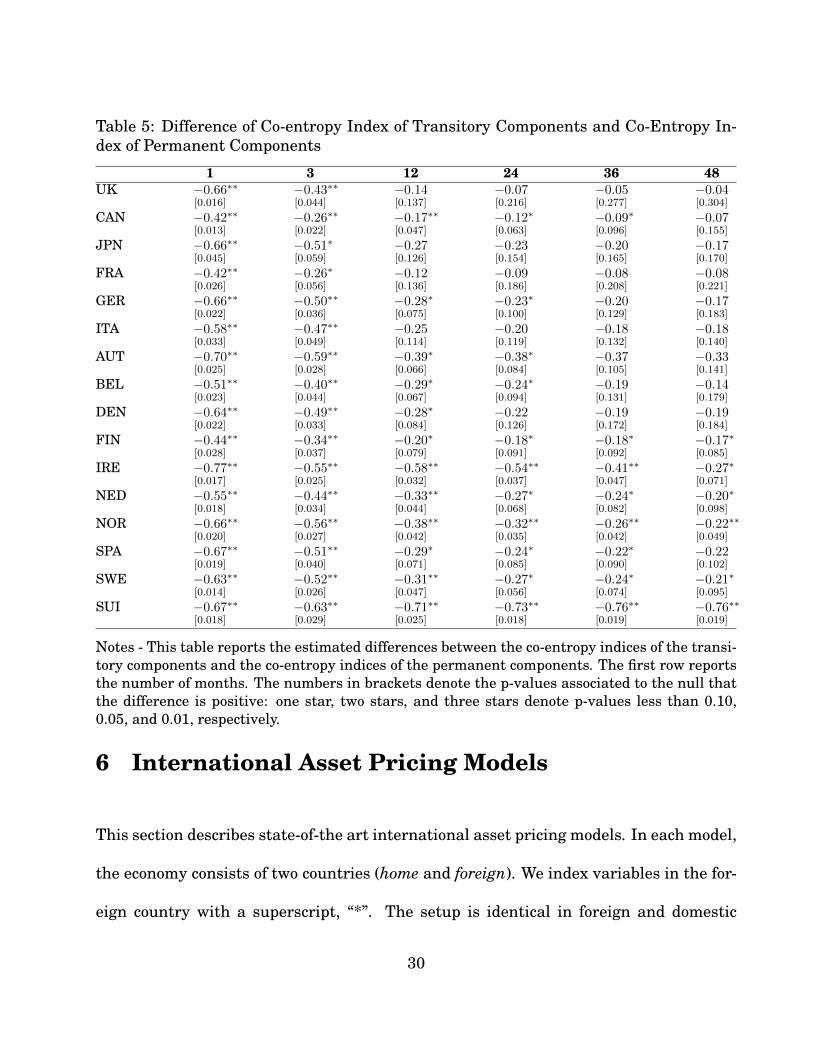
Table 5: Difference of Co-entropy Index of Transitory Components and Co-Entropy In-dex of Permanent Components

1 3 12 24 36 48UK −0.66∗∗ −0.43∗∗ −0.14 −0.07 −0.05 −0.04

[0.016] [0.044] [0.137] [0.216] [0.277] [0.304]

CAN −0.42∗∗ −0.26∗∗ −0.17∗∗ −0.12∗ −0.09∗ −0.07[0.013] [0.022] [0.047] [0.063] [0.096] [0.155]

JPN −0.66∗∗ −0.51∗ −0.27 −0.23 −0.20 −0.17[0.045] [0.059] [0.126] [0.154] [0.165] [0.170]

FRA −0.42∗∗ −0.26∗ −0.12 −0.09 −0.08 −0.08[0.026] [0.056] [0.136] [0.186] [0.208] [0.221]

GER −0.66∗∗ −0.50∗∗ −0.28∗ −0.23∗ −0.20 −0.17[0.022] [0.036] [0.075] [0.100] [0.129] [0.183]

ITA −0.58∗∗ −0.47∗∗ −0.25 −0.20 −0.18 −0.18[0.033] [0.049] [0.114] [0.119] [0.132] [0.140]

AUT −0.70∗∗ −0.59∗∗ −0.39∗ −0.38∗ −0.37 −0.33[0.025] [0.028] [0.066] [0.084] [0.105] [0.141]

BEL −0.51∗∗ −0.40∗∗ −0.29∗ −0.24∗ −0.19 −0.14[0.023] [0.044] [0.067] [0.094] [0.131] [0.179]

DEN −0.64∗∗ −0.49∗∗ −0.28∗ −0.22 −0.19 −0.19[0.022] [0.033] [0.084] [0.126] [0.172] [0.184]

FIN −0.44∗∗ −0.34∗∗ −0.20∗ −0.18∗ −0.18∗ −0.17∗

[0.028] [0.037] [0.079] [0.091] [0.092] [0.085]

IRE −0.77∗∗ −0.55∗∗ −0.58∗∗ −0.54∗∗ −0.41∗∗ −0.27∗

[0.017] [0.025] [0.032] [0.037] [0.047] [0.071]

NED −0.55∗∗ −0.44∗∗ −0.33∗∗ −0.27∗ −0.24∗ −0.20∗

[0.018] [0.034] [0.044] [0.068] [0.082] [0.098]

NOR −0.66∗∗ −0.56∗∗ −0.38∗∗ −0.32∗∗ −0.26∗∗ −0.22∗∗

[0.020] [0.027] [0.042] [0.035] [0.042] [0.049]

SPA −0.67∗∗ −0.51∗∗ −0.29∗ −0.24∗ −0.22∗ −0.22[0.019] [0.040] [0.071] [0.085] [0.090] [0.102]

SWE −0.63∗∗ −0.52∗∗ −0.31∗∗ −0.27∗ −0.24∗ −0.21∗

[0.014] [0.026] [0.047] [0.056] [0.074] [0.095]

SUI −0.67∗∗ −0.63∗∗ −0.71∗∗ −0.73∗∗ −0.76∗∗ −0.76∗∗

[0.018] [0.029] [0.025] [0.018] [0.019] [0.019]

Notes - This table reports the estimated differences between the co-entropy indices of the transi-tory components and the co-entropy indices of the permanent components. The first row reportsthe number of months. The numbers in brackets denote the p-values associated to the null thatthe difference is positive: one star, two stars, and three stars denote p-values less than 0.10,0.05, and 0.01, respectively.

6 International Asset Pricing Models

This section describes state-of-the art international asset pricing models. In each model,

the economy consists of two countries (home and foreign). We index variables in the for-

eign country with a superscript, “*”. The setup is identical in foreign and domestic

30

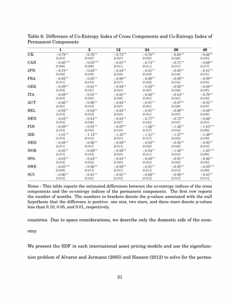
Table 6: Difference of Co-Entropy Index of Cross Components and Co-Entropy Index ofPermanent Components

1 3 12 24 36 48UK −0.78∗∗ −0.76∗∗ −0.73∗∗ −0.70∗∗ −0.68∗∗ −0.66∗∗

[0.014] [0.027] [0.027] [0.025] [0.026] [0.023]

CAN −0.80∗∗∗ −0.85∗∗∗ −0.81∗∗ −0.74∗∗ −0.71∗∗ −0.68∗∗

[0.006] [0.006] [0.011] [0.011] [0.015] [0.017]

JPN −0.78∗∗ −0.82∗∗ −0.84∗∗ −0.81∗∗ −0.80∗∗ −0.81∗∗

[0.038] [0.039] [0.049] [0.049] [0.046] [0.041]

FRA −0.92∗∗ −0.95∗∗ −0.98∗∗ −0.98∗∗ −0.99∗∗ −0.99∗∗

[0.011] [0.018] [0.017] [0.020] [0.018] [0.016]

GER −0.89∗∗ −0.91∗∗ −0.94∗∗ −0.92∗∗ −0.92∗∗ −0.88∗∗

[0.016] [0.021] [0.023] [0.027] [0.026] [0.025]

ITA −0.89∗∗ −0.91∗∗ −0.91∗∗ −0.88∗∗ −0.84∗∗ −0.78∗∗

[0.023] [0.025] [0.036] [0.031] [0.031] [0.032]

AUT −0.86∗∗ −0.90∗∗ −0.94∗∗ −0.91∗∗ −0.87∗∗ −0.82∗∗

[0.021] [0.018] [0.027] [0.031] [0.029] [0.037]

BEL −0.92∗∗ −0.93∗∗ −0.94∗∗ −0.91∗∗ −0.90∗∗ −0.88∗∗

[0.013] [0.019] [0.019] [0.021] [0.027] [0.028]

DEN −0.83∗∗ −0.84∗∗ −0.84∗∗ −0.77∗∗ −0.72∗∗ −0.66∗

[0.016] [0.020] [0.027] [0.035] [0.047] [0.054]

FIN −0.89∗∗ −0.91∗∗ −0.97∗∗ −1.06∗∗ −1.36∗∗ −1.83∗∗∗

[0.014] [0.016] [0.018] [0.017] [0.016] [0.008]

IRE −1.01∗∗ −1.13∗∗ −1.25∗∗ −1.21∗∗ −1.27∗∗ −1.39∗∗

[0.013] [0.013] [0.015] [0.017] [0.023] [0.039]

NED −0.88∗∗ −0.90∗∗ −0.93∗∗ −0.92∗∗ −0.92∗∗ −0.92∗∗

[0.011] [0.017] [0.014] [0.020] [0.020] [0.018]

NOR −0.85∗∗ −0.89∗∗ −0.93∗∗ −0.94∗∗ −1.00∗∗ −1.05∗∗∗

[0.015] [0.016] [0.016] [0.011] [0.010] [0.008]

SPA −0.83∗∗ −0.83∗∗ −0.84∗∗ −0.89∗∗ −0.91∗∗ −0.86∗∗

[0.016] [0.024] [0.023] [0.024] [0.023] [0.024]

SWE −0.85∗∗∗ −0.90∗∗ −0.93∗∗ −0.91∗∗ −0.92∗∗ −0.89∗∗∗

[0.009] [0.014] [0.015] [0.014] [0.014] [0.009]

SUI −0.90∗∗ −0.91∗∗ −0.91∗∗ −0.89∗∗ −0.90∗∗ −0.85∗∗

[0.013] [0.021] [0.019] [0.012] [0.013] [0.014]

Notes - This table reports the estimated differences between the co-entropy indices of the crosscomponents and the co-entropy indices of the permanent components. The first row reportsthe number of months. The numbers in brackets denote the p-values associated with the nullhypothesis that the difference is positive: one star, two stars, and three stars denote p-valuesless than 0.10, 0.05, and 0.01, respectively.

countries. Due to space considerations, we describe only the domestic side of the econ-

omy.

We present the SDF in each international asset pricing models and use the eigenfunc-

tion problem of Alvarez and Jermann (2005) and Hansen (2012) to solve for the perma-

31

nent and transitory components of SDFs. For more details, we refer readers to each

model. We keep the same notations as in the original models to facilitate comparisons.

The parameter values used are specific to each model and have no analogous meaning to

other models. The choice of the models is guided by their success in explaining several

features of international asset pricing quantities and puzzles.

The main finding is the same for all models. While they are all successful in accounting

for the degree of codependence of the stochastic discount factors (which is what most of

these models were designed to do), they all seem to struggle in reproducing the right mix

of entropy-based correlations for the permanent and transitory components of SDFs. In

general, it seems to be the case that all the models overshoot, in terms of the contribu-

tion of the correlation of the transitory components at horizons less than one year, and

cannot reproduce the upward sloping term structure of co-entropy of these components.

6.1 A Model with Long-Run Risks

Setup of the economy. This model follows the setup described by Colacito and Croce

(2011) and Colacito (2012).5 Agents order consumption profiles according to the follow-

ing utility function:

Ut = (1− δ) logCt + δθ logEt exp

{Ut+1

θ

}, (22)

5More recently, Lewis and Liu (2012), Bansal and Shaliastovich (forthcoming), and Zviadadze (2013)have also built on this international version of the Bansal and Yaron (2004) long-run risks model.

32

where θ = 1/(1− γ), γ is the coefficient of risk aversion, and δ is the subjective discount

factor. The logarithm of the growth rate of consumption follows this process:

logCt+1

Ct= ∆ct+1 = µc + xt + σcεc,t+1, (23)

xt = ρxt−1 + σxεx,t,

where εc,t+1 and εx,t+1 are jointly normally distributed as independent standard normals.

While shocks are orthogonal within each country, we allow them to be correlated across

countries. Specifically, we let ρx,x∗ and ρc,c∗ denote the cross-country correlations of the

shocks to x and ∆c, respectively, and ρc,x∗ denote the correlation between shocks to x in

one country and shocks to ∆c in the other country.

Stochastic discount factor and its components. We solve the eigenfunction prob-

lem of Alvarez and Jermann (2005) and Hansen (2012) and show (see Online Appendix

I) that the logarithms of SDF, and its permanent and transitory components can be

expressed as follows:

mt+1 = log δ − µc −B2σ2

x

2θ2− σ2

c

2θ2− xt +

Bσxθεx,t+1 +

(1

θ− 1

)σcεc,t+1, (24)

mTt+1 = log (ζ)− xt − ξσxεx,t+1,

mPt+1 =

(B

θ+ ξ

)σxεx,t+1 +

(1

θ− 1

)σcεc,t+1 −

1

2

(B

θ+ ξ

)2

σ2x −

1

2

(1

θ− 1

)2

σ2c ,

33

with B = δ/(1− δρ), ξ = 1/ (ρ− 1) and

log (ζ) = log δ − µc −B2σ2

x

2θ2− σ2

c

2θ2+

1

2

(Bσxθ

+1

ρ− 1σx

)2

+1

2

(1

θ− 1

)2

σ2c .

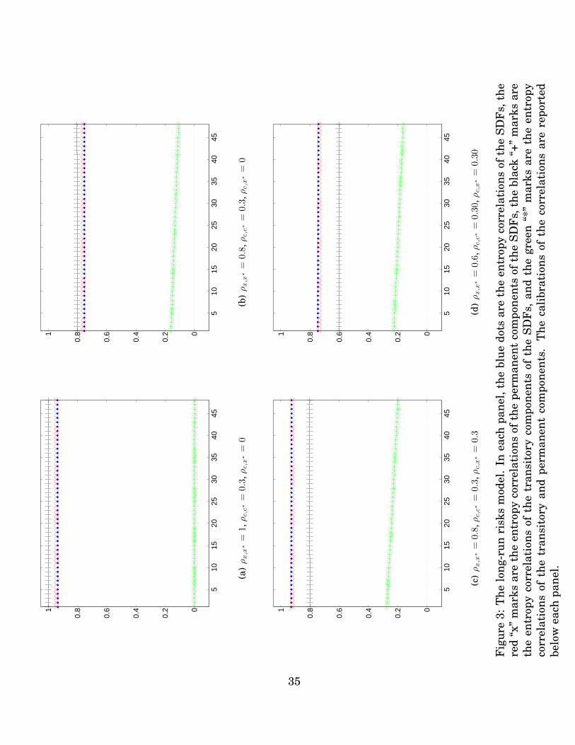
Discussion. Figure 3 reports the results of some alternative calibrations of the inter-

national correlations of the shocks. Risk aversion γ is set to 10, while the elasticity of

intertemporal substitution, ψ, is equal to 1. All other parameters are set to the same

numbers of the original paper. Panel (a) refers to the baseline calibration, according to

which the predictive components of consumption growth rates are perfectly correlated

across countries. This clearly results in an overstatement of the role of the codependence

of the transitory components, while all other entropy-based correlations appear to be in

line with the data.

The issue of the excessive codependence of the transitory components in this model

can be mitigated by lowering the correlation of long-run risks, while offsetting such

reduction with an increase in the correlation between the long-run shocks in one country

and the short-run shocks in the other (see panel (c)).6 This choice of parameters appears

to enable the model to replicate the average degrees of correlations across all horizons,

but it still falls short of accounting for the upward sloping term structure of co-entropy

of the transitory components that we observe in the data.

6Colacito (2012) also argues in favor of such calibration to better account for the imperfect degree ofcorrelation of interest rates across major industrialized countries.

34

510

1520

2530

3540

45

0

0.2

0.4

0.6

0.81

(a)ρx,x

∗=

1,ρc,c

∗=

0.3,ρc,x

∗=

0

510

1520

2530

3540

45

0

0.2

0.4

0.6

0.81

(b)ρx,x

∗=

0.8,ρc,c

∗=

0.3,ρ

c,x

∗=

0

510

1520

2530

3540

45

0

0.2

0.4

0.6

0.81

(c)ρx,x

∗=

0.8,ρc,c

∗=

0.3,ρc,x

∗=

0.3

510

1520

2530

3540

45

0

0.2

0.4

0.6

0.81

(d)ρx,x

∗=

0.6,ρc,c

∗=

0.30,ρ

c,x

∗=

0.30

Fig

ure

3:T

helo

ng-r

unri

sks

mod

el.

Inea

chpa

nel,

the

blue

dots

are

the

entr

opy

corr

elat

ions

ofth

eSD

Fs,

the

red

“x”

mar

ksar

eth

een

trop

yco

rrel

atio

nsof

the

perm

anen

tco

mpo

nent

sof

the

SDF

s,th

ebl

ack

“+”

mar

ksar

eth

een

trop

yco

rrel

atio

nsof

the

tran

sito

ryco

mpo

nent

sof

the

SDF

s,an

dth

egr

een

“*”

mar

ksar

eth

een

trop

yco

rrel

atio

nsof

the

tran

sito

ryan

dpe

rman

ent

com

pone

nts.

The

calib

rati

ons

ofth

eco

rrel

atio

nsar

ere

port

edbe

low

each

pane

l.

35

6.2 A Model with Habits

Setup of the Economy. In this section, we consider the two-country model with exter-

nal habits of Verdelhan (2010). Agents order consumption streams and maximize their

expected utility (see also Campbell and Cochrane (1999))

E∞∑t=0

βt(Ct −Ht)

1−γ − 1

1− γ, (25)

where γ is the risk-aversion coefficient, Ht is the external habit level, and Ct is the

agent’s consumption. Define St = Ct−Ht

Ctas the surplus consumption ratio, and st =

log (St). The consumption growth is log-normally distributed ∆ct+1 = g+ut+1 with ut+1 v

N (0, σ2). We denote by ρu,u∗ the cross-country correlation of the endowment shocks. The

sensitivity function λ (st) governs the dynamics of the surplus consumption ratio

λ (st) = 1S

√1− 2 (st − s)− 1 , when st ≤ smax and 0 elsewhere (26)

and the dynamic of the surplus consumption ratio is given by

st+1 ≡ (1− φ) s+ φst + λ (st)ut+1,

with smax = s+ 12

(1− S2

).

Stochastic discount factor and its components. In Online Appendix II, we solve the

36

eigenfunction problem and derive the permanent and transitory components of SDFs.

The logarithms of the SDF and its permanent and transitory components can be ex-

pressed as follows:

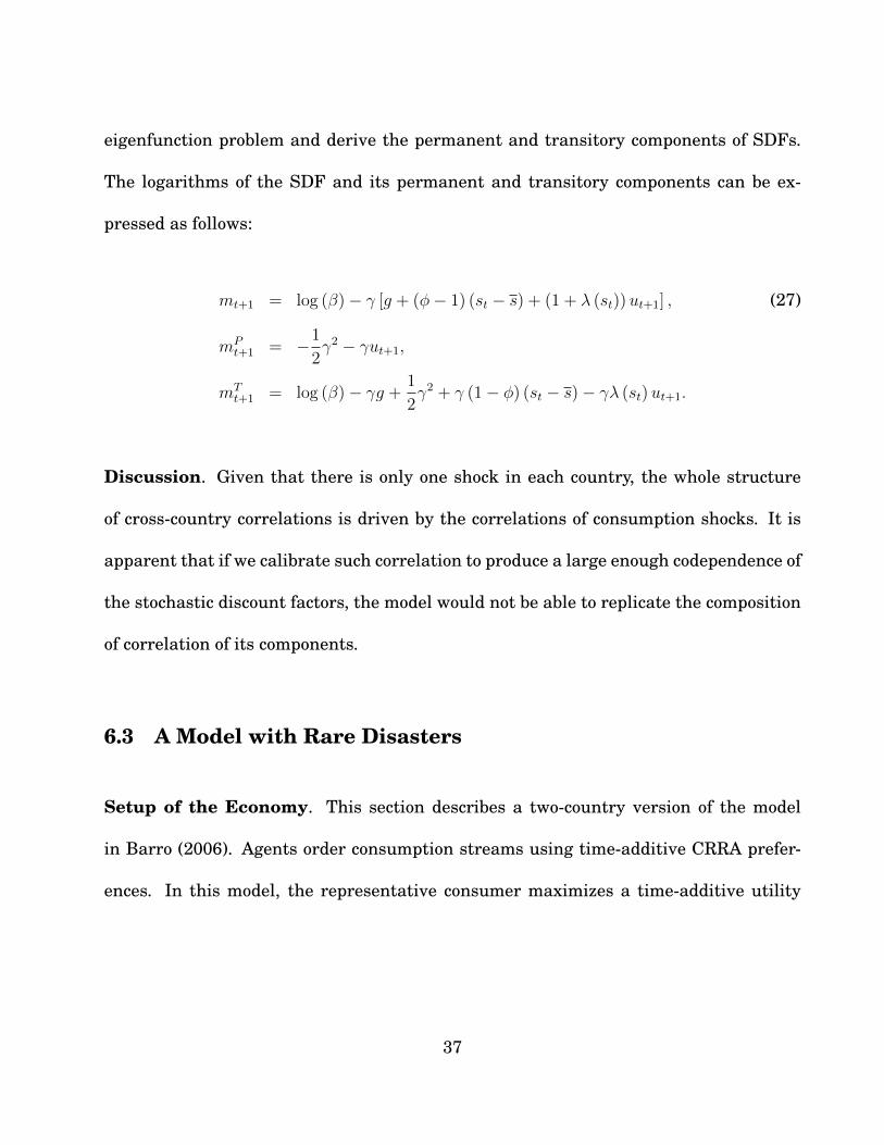
mt+1 = log (β)− γ [g + (φ− 1) (st − s) + (1 + λ (st))ut+1] , (27)

mPt+1 = −1

2γ2 − γut+1,

mTt+1 = log (β)− γg +

1

2γ2 + γ (1− φ) (st − s)− γλ (st)ut+1.

Discussion. Given that there is only one shock in each country, the whole structure

of cross-country correlations is driven by the correlations of consumption shocks. It is

apparent that if we calibrate such correlation to produce a large enough codependence of

the stochastic discount factors, the model would not be able to replicate the composition

of correlation of its components.

6.3 A Model with Rare Disasters

Setup of the Economy. This section describes a two-country version of the model

in Barro (2006). Agents order consumption streams using time-additive CRRA prefer-

ences. In this model, the representative consumer maximizes a time-additive utility

37

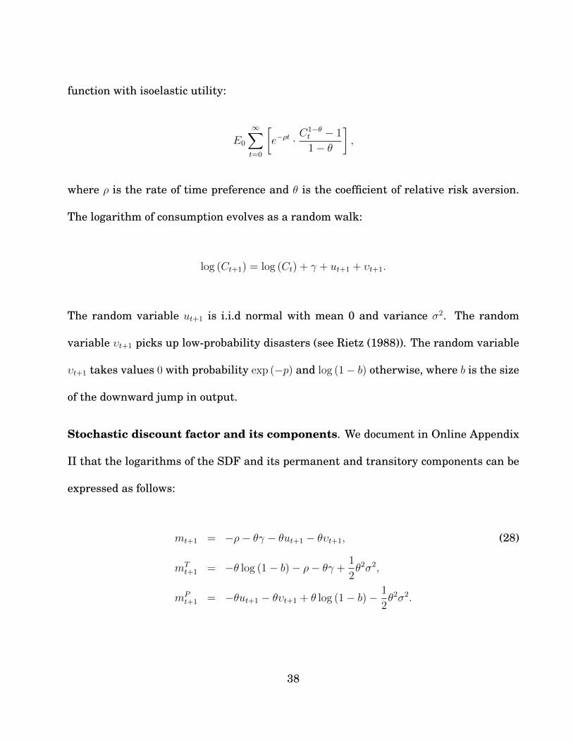
function with isoelastic utility:

E0

∞∑t=0

[e−ρt · C

1−θt − 1

1− θ

],

where ρ is the rate of time preference and θ is the coefficient of relative risk aversion.

The logarithm of consumption evolves as a random walk:

log (Ct+1) = log (Ct) + γ + ut+1 + υt+1.

The random variable ut+1 is i.i.d normal with mean 0 and variance σ2. The random

variable υt+1 picks up low-probability disasters (see Rietz (1988)). The random variable

υt+1 takes values 0 with probability exp (−p) and log (1− b) otherwise, where b is the size

of the downward jump in output.

Stochastic discount factor and its components. We document in Online Appendix

II that the logarithms of the SDF and its permanent and transitory components can be

expressed as follows:

mt+1 = −ρ− θγ − θut+1 − θυt+1, (28)

mTt+1 = −θ log (1− b)− ρ− θγ +

1

2θ2σ2,

mPt+1 = −θut+1 − θυt+1 + θ log (1− b)− 1

2θ2σ2.

38

Discussion. Figure 4 reports the entropy correlations for this model. We calibrate all

the parameters according to the original paper. Furthermore, we set the international

correlation of the non disaster shocks to consumption to 0.3 and the correlation of the

disaster shocks to 1. We document the performance of the model for three alternative

values of the disaster’s intensity.

The results are quite intuitive. Since disasters are perfectly correlated across coun-

tries, as the consumption loss in case of disaster increases, so does the correlation of the

stochastic discount factors. This upward shift is accompanied one for one by an increase

in the correlation of the permanent components. Given that growth rates are i.i.d. and

homoskedastic, interest rates are constant in the model. This implies that the entropy

correlation of the transitory component is always equal to 1 and the entropy correla-

tion of the ratio of permanent and the ratio of transitory components is always equal to

0, regardless of the calibration. In sum, this model cannot overcome the shortcomings

already discussed in the context of the earlier models.

39

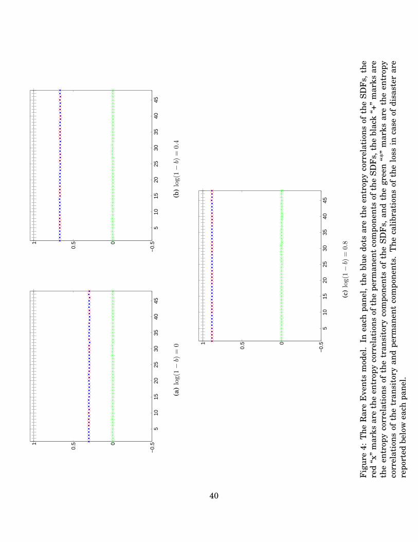
510

1520

2530

3540

45−

0.50

0.51

(a)

log(1−b)

=0

510

1520

2530

3540

45−

0.50

0.51

(b)

log(1−b)

=0.

4

510

1520

2530

3540

45−

0.50

0.51

(c)

log(1−b)

=0.

8

Fig

ure

4:T

heR

are

Eve

nts

mod

el.

Inea

chpa

nel,

the

blue

dots

are

the

entr

opy

corr

elat

ions

ofth

eSD

Fs,

the

red

“x”

mar

ksar

eth

een

trop

yco

rrel

atio

nsof

the

perm

anen

tco

mpo

nent

sof

the

SDF

s,th

ebl

ack

“+”

mar

ksar

eth

een

trop

yco

rrel

atio

nsof

the

tran

sito

ryco

mpo

nent

sof

the

SDF

s,an

dth

egr

een

“*”

mar

ksar

eth

een

trop

yco

rrel

atio

nsof

the

tran

sito

ryan

dpe

rman

ent

com

pone

nts.

The

calib

rati

ons

ofth

elo

ssin

case

ofdi

sast

erar

ere

port

edbe

low

each

pane

l.

40

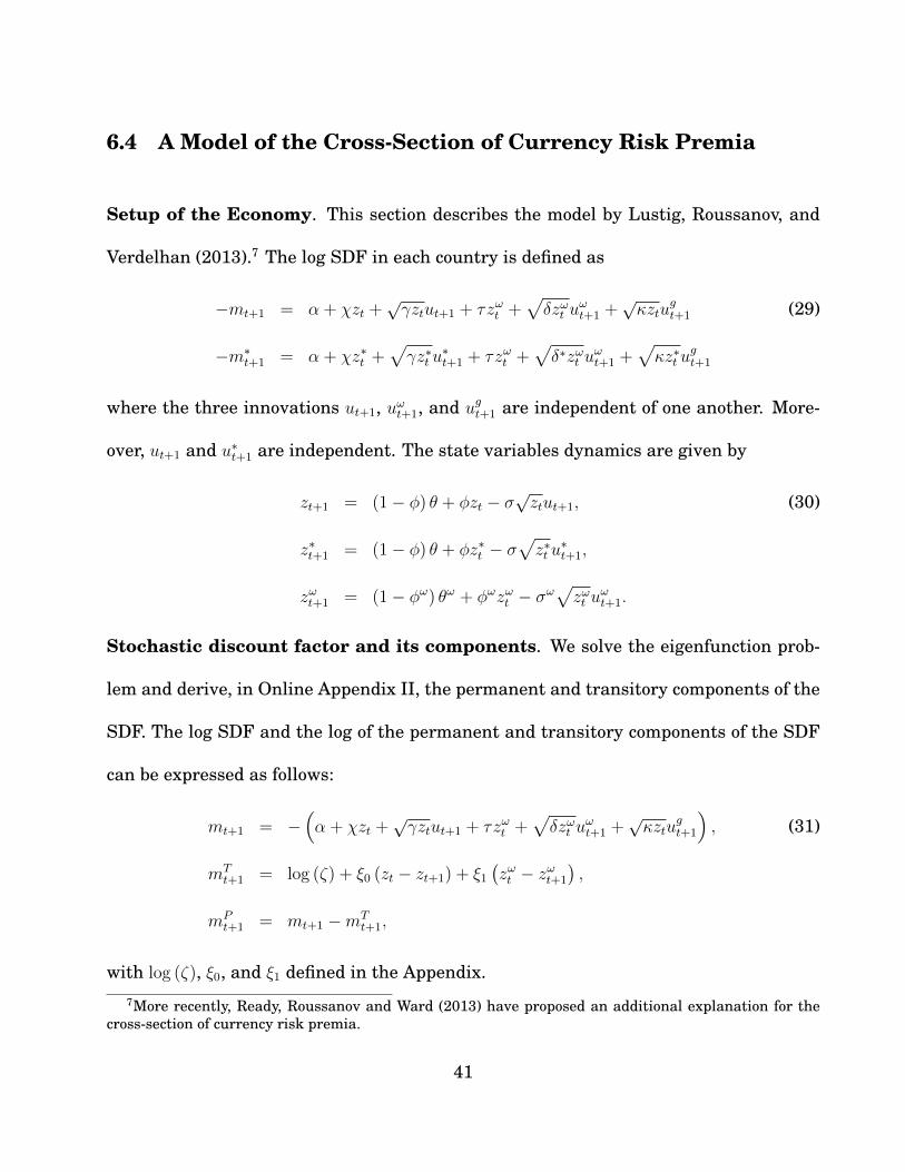
6.4 A Model of the Cross-Section of Currency Risk Premia

Setup of the Economy. This section describes the model by Lustig, Roussanov, and

Verdelhan (2013).7 The log SDF in each country is defined as

−mt+1 = α + χzt +√γztut+1 + τzωt +

√δzωt u

ωt+1 +

√κztu

gt+1 (29)

−m∗t+1 = α + χz∗t +√γz∗t u

∗t+1 + τzωt +

√δ∗zωt u

ωt+1 +

√κz∗t u

gt+1

where the three innovations ut+1, uωt+1, and ugt+1 are independent of one another. More-

over, ut+1 and u∗t+1 are independent. The state variables dynamics are given by

zt+1 = (1− φ) θ + φzt − σ√ztut+1, (30)

z∗t+1 = (1− φ) θ + φz∗t − σ√z∗t u

∗t+1,

zωt+1 = (1− φω) θω + φωzωt − σω√zωt u

ωt+1.

Stochastic discount factor and its components. We solve the eigenfunction prob-

lem and derive, in Online Appendix II, the permanent and transitory components of the

SDF. The log SDF and the log of the permanent and transitory components of the SDF

can be expressed as follows:

mt+1 = −(α + χzt +

√γztut+1 + τzωt +

√δzωt u

ωt+1 +

√κztu

gt+1

), (31)

mTt+1 = log (ζ) + ξ0 (zt − zt+1) + ξ1

(zωt − zωt+1

),

mPt+1 = mt+1 −mT

t+1,

with log (ζ), ξ0, and ξ1 defined in the Appendix.7More recently, Ready, Roussanov and Ward (2013) have proposed an additional explanation for the

cross-section of currency risk premia.

41

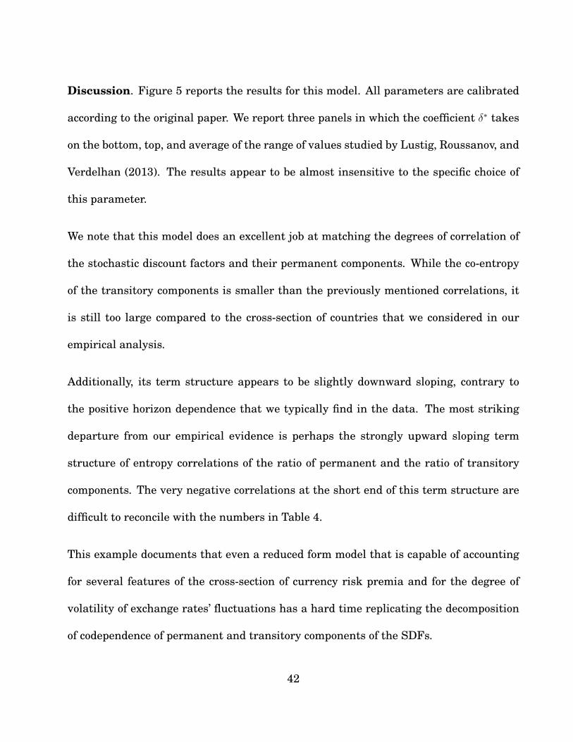
Discussion. Figure 5 reports the results for this model. All parameters are calibrated

according to the original paper. We report three panels in which the coefficient δ∗ takes

on the bottom, top, and average of the range of values studied by Lustig, Roussanov, and

Verdelhan (2013). The results appear to be almost insensitive to the specific choice of

this parameter.

We note that this model does an excellent job at matching the degrees of correlation of

the stochastic discount factors and their permanent components. While the co-entropy

of the transitory components is smaller than the previously mentioned correlations, it

is still too large compared to the cross-section of countries that we considered in our

empirical analysis.

Additionally, its term structure appears to be slightly downward sloping, contrary to

the positive horizon dependence that we typically find in the data. The most striking

departure from our empirical evidence is perhaps the strongly upward sloping term

structure of entropy correlations of the ratio of permanent and the ratio of transitory

components. The very negative correlations at the short end of this term structure are

difficult to reconcile with the numbers in Table 4.

This example documents that even a reduced form model that is capable of accounting

for several features of the cross-section of currency risk premia and for the degree of

volatility of exchange rates’ fluctuations has a hard time replicating the decomposition

of codependence of permanent and transitory components of the SDFs.

42

510

1520

2530

3540

45−

0.50

0.51

(a)δ

=10

,δ∗

=7.

71

510

1520

2530

3540

45−

0.50

0.51

(b)δ

=10,δ∗

=12.

29

510

1520

2530

3540

45−

0.50

0.51

(c)δ

=δ∗

=10

Fig

ure

5:T

heL

RV

mod

el.

Inea

chpa

nel,

the

blue

dots

are

the

entr

opy

corr

elat

ions

ofth

eSD

Fs,

the

red

“x”

mar

ksar

eth

een

trop

yco

rrel

atio

nsof

the

perm

anen

tco

mpo

nent

sof

the

SDF

s,th

ebl

ack

“+”

mar

ksar

eth

een

trop

yco

rrel

atio

nsof

the

tran

sito

ryco

mpo

nent

sof

the

SDF

s,an

dth

egr

een

“*”

mar

ksar

eth

een

trop

yco

rrel

atio

nsof

the

tran

sito

ryan

dpe

rman

ent

com

pone

nts.

The

calib

rati

ons

ofth

eex

posu

res

toth

ew

orld

fact

orar

ere

port

edbe

low

each

pane

l.

43

6.5 A Potential Resolution: Intertemporal Correlation of the Shocks

The common assumption of the models discussed up to this point is that shocks are i.i.d.

across dates. One possible resolution for the shortcomings of the models discussed in

this section consists in letting shocks be correlated across time. In this subsection we

propose a small amendment of the model with the long-run risks discussed in section 6.1,

with the understanding that this generalization could be extended to the other models

that we have investigated so far.

Following the notation of section 6.1, we allow for three additional sources of correlation:

ρlagx,x∗ = corr(εx,t, ε

∗x,t−1

)= corr

(εx,t−1, ε

∗x,t

),

ρlagc,c∗ = corr(εc,t, ε

∗c,t−1

)= corr

(εc,t−1, ε

∗c,t

),

ρlagc,x∗ = corr(εc,t, ε

∗x,t−1

)= corr

(εc,t−1, ε

∗x,t

).

The introduction of these intertemporal correlations does not affect the decomposition

of the stochastic discount factors into permanent and transitory components in (24).

This is because the additional correlations only involve the cross-country correlations of

shocks, while leaving the dynamics within each country unaffected.

Figure 6 presents the results associated with this model. The choice of parameters’

values is reported in the note to the figure. The correlations of the shocks are chosen in

order to minimize the squared differences between the term structures of co-entropies in

the model and in the data for the US and the UK. Note that when the model is allowed

44

to choose the term structure of correlations that best fits the data, it will decrease the

contemporaneous correlation of long-run risks and compensate this with an increase in

the intertemporal correlation of these shocks across countries. Additionally, note that

the correlation between the long-run shocks in one country and the short-run shocks in

the other country are quite large.

The resulting term structure of correlations of the transitory components is now sharply

upward sloping, in line with what we found in the data. The model now also features

positive horizon codependence of the stochastic discount factors and their permanent

components. While these appear to be at odds with the empirical evidence reported in

section 5, we note from Table 1 and Table 2 that these co-entropies are usually within

the 95% confidence intervals, with the only possible exception of very short horizons.

Overall, while this model represents a significant step forward, relative to the other

models discussed in this section, there still seems to be a tension between the ability of

generating a positive horizon codependence of transitory components and matching the

empirical evidence on the virtually flat term structures of all other co-entropies.

We take the simple exercise of this section as suggesting the relevance of modeling in-

tertemporal correlations. From a technical point of view, this appears to be a necessary

step toward a better replication of the term structure of co-entropies in international

financial markets. In terms of economic modeling, this evidence suggests that more

attention should be focused on understanding the mechanism through which shocks

45

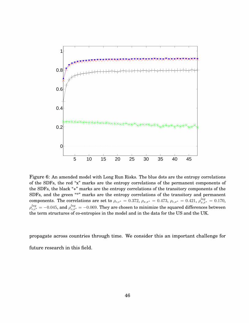
5 10 15 20 25 30 35 40 45

0

0.2

0.4

0.6

0.8

1

Figure 6: An amended model with Long Run Risks. The blue dots are the entropy correlationsof the SDFs, the red “x” marks are the entropy correlations of the permanent components ofthe SDFs, the black “+” marks are the entropy correlations of the transitory components of theSDFs, and the green “*” marks are the entropy correlations of the transitory and permanentcomponents. The correlations are set to ρc,c∗ = 0.372, ρx,x∗ = 0.473, ρc,x∗ = 0.421, ρlagx,x∗ = 0.170,ρlagc,c∗ = −0.045, and ρlagc,x∗ = −0.069. They are chosen to minimize the squared differences betweenthe term structures of co-entropies in the model and in the data for the US and the UK.

propagate across countries through time. We consider this an important challenge for

future research in this field.

46

7 Concluding Remarks

The common feature across the models that we analyzed appears to be the general abil-

ity of accounting for the large degree of co-entropy (codependence) of the stochastic

discount factors, whether coming from a high correlation of long-run risks, a common

disaster state, exposure to a world risk factor, etc. Our analysis reveals that, while this

major task can be accomplished through a variety of models, reproducing the composi-

tion of co-entropy is still very difficult for these state-of-the-art models.

In particular, it seems to be the case that economic models rely heavily on the correlation

of transitory components. If, on the one hand, this hypothesis cannot be rejected at

longer horizons, on the other hand, it is hard to reconcile with our empirical evidence

from a large cross-section of major industrialized countries.

Perhaps even more interesting are the level and the term structure of co-entropy of

transitory components across countries. The data reveal that transitory shocks display

a significant and increasing degree of codependence through time, a robust finding for

an overwhelming majority of developed countries in our sample. Existing international

asset pricing models feature a very high level of co-entropy and a flat term structure

of co-entropies of transitory components across countries. In addition, some models are

not able to reproduce level and slope of the term structure of the co-entropy between the

ratio of permanent components across countries and the ratio of transitory components.

47

Taken together, these findings seem to suggest that future research should devote more

attention to the temporal distribution of correlations. Our analysis reveals the need of

paying more attention to the intertemporal distribution of co-movement between var-

ious components of the SDFs across countries, as opposed to the contemporaneous co-

movement of shocks. While the former has typically been neglected in existing models,

the latter has been carrying all the weight to deliver a high degree of correlation co-

movement of the stochastic discount factors.

This is an important direction for future research, as it requires a deeper understanding

about the way in which shocks of different nature are shared internationally across

time and about the timing with which technological, preference, and endowment shocks

spread across countries. General equilibrium models of the likes of Pavlova and Rigobon

(2007) are now faced with a tighter set of constraints, which will perhaps allow us to gain

a deeper understanding of the sources of risk in international macro-finance models.

48

ReferencesAlvarez, Fernando and Urban Jermann, “Using Asset Prices to Measure the Persistence of

the Marginal Utility of Wealth,” Econometrica, 2005, 73, 1977–2016.

Backus, D, M Chernov, and I Martin, “Disasters implied by equity index options,” Journal ofFinance, 2011, 66, 1969–2012.

Backus, David, Mikhail Chernov, and Stanley Zin, “Sources of entropy in representativeagent models,” Journal of Finance (forthcoming), 2013.

Bakshi, Gurdip and Fousseni Chabi-Yo, “Variance bounds on the permanent and transitorycomponents of stochastic discount factors,” Journal of Financial Economics, 2012, 105, 191–208.

and , “New Entropy Restrictions and the Quest for Better Specified Asset PricingModels,” Working paper, Ohio State University 2013.

Bansal, R. and Ivan Shaliastovich, “A Long-Run Risks Explanation of Predictability Puzzlesin Bond and Currency Markets,” Review of Financial Studies, forthcoming.

Bansal, Ravi and Amir Yaron, “Risks for the Long Run: A Potential Resolution of AssetPricing Puzzles,” Journal of Finance, 2004, 59, 1481–1509.

and Bruce Lehmann, “Growth-Optimal Portfolio Restrictions on Asset Pricing Models,”Macroeconomic Dynamics, 1997, 1, 333–354.

Barro, Robert, “Rare Disasters and Asset Markets in the Twentieth Century,” Quarterly Jour-nal of Economics, 2006, 121 (9), 823–866.

Borovicka, Jaroslav and Lars Hansen, “Examining Macroeconomic Models through the Lensof Asset Pricing?,” Journal of Econometrics (forthcoming), 2013.

Brandt, Michael, John Cochrane, and Pedro Santa-Clara, “International Risk Sharingis Better Than You Think, or Exchange Rates are Too Smooth,” Journal of Monetary Eco-nomics, 2006, 53, 671–698.

Campbell, J. and J. Cochrane, “Force of Habit: A Consumption-Based Explanation of Aggre-gate Stock Market Behavior,” Journal of Political Economy, 1999, 107, 205–251.

Colacito, Riccardo, “Six anomalies looking for a model. A consumption based explanation ofinternational finance puzzles.,” Working Paper, Department of Finance, University of NorthCarolina, Chapel Hill NC, 2012.

and Mariano M. Croce, “Risks for the long run and the real exchange rate,” Journal ofPolitical Economy, 2011, 19(1), 223–250.

Gavazzoni, F., B. Sambalaibat, and C. Telmer, “Currency Risk and Pricing Kernel Volatility,”Carnegie Mellon University and INSEAD Working Paper, 2013.

Hansen, L and J Scheinkman, “Long-Term Risk: An Operator Approach,” Econometrica,2009, 77, 177–234.

, J Heaton, and N Li, “Consumption Strikes Back? Measuring Long-Run Risk,” Journalof Political Economy, 2008, 116, 260–302.

Hansen, Lars, “Dynamic value decomposition in stochastic economies,” Econometrica, 2012, 80,911–967.

49

, Handbook of the Economics of Finance, New York, NY: North-Holland, 2013.

and Ravi Jagannathan, “Implications of Security Market Data for Dynamic Economies,”Journal of Political Economy, 1991, 99, 225–261.

Jotikasthira, Pab, Anh Le, and Chris Lundblad, “Why Do Term Structures in DifferentCurrencies Comove?,” Working Paper UNC Chapel Hill, 2013.

Koijen, Ralph, Hanno Lustig, and Stijn Van Nieuwerburgh, “The Cross-Section and Time-Series of Stock and Bond Returns,” Unpublished Working Paper, NBER # 15688 2010.

Lewis, Karen and Edith Liu, “International Consumption Risk is Shared After All: An AssetReturn View,” Working Paper, University of Pennsylvania and Cornell University, 2012.

Lustig, Hanno, Andreas Stathopoulos, and Adrien Verdelhan, “The Term Structure ofCurrency Carry Trade Risk Premia,” MIT, UCLA, and USC Working Paper, 2013.

, Nikolai Roussanov, and Adrien Verdelhan, “Countercyclical Currency Risk Premia,”Journal of Financial Economics (forthcoming), 2013.

Martin, Ian, “Consumption-Based Asset Pricing with Higher Cumulants,” Review of EconomicStudies, 2013, 80, 745–773.

Pavlova, Anna and Roberto Rigobon, “Asset Prices and Exchange Rates,” Review of Finan-cial Studies, 2007, 20(4), 1139–1181.

Ready, Robert, Nick Roussanov, and Colin Ward, “Commodity Trade and the Carry Trade:a Tale of Two Countries,” Working Paper, University of Pennsylvania and Rochester Univer-sity, 2013.

Rietz, T, “The equity risk premium: A solution,” Journal of Monetary Economics, 1988, 22,117–131.

van Binsbergen, Jules H., Michael W. Brandt, and Ralph Koijen, “On the Timing andPricing of Dividends,” American Economic Review, 2012, 102(4), 1596–1618.

, Wouter Hueskes, Ralph Koijen, and Evert B. Vrugt, “Equity Yields,” Journal of Fi-nancial Economics, 2013, p. forthcoming.

Verdelhan, Adrien, “A Habit-Based Explanation of the Exchange Rate Risk Premium,” Journalof Finance, Vol. 65, No 1, pp 123-145, 2010.

Zviadadze, Irina, “Term-Structure of Consumption Risk Premia in the Cross-Section of Cur-rency Returns,” Working Paper Stockholm School of Economics, 2013.

50

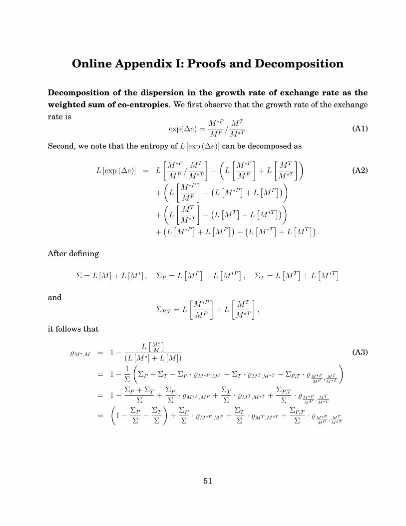
Online Appendix I: Proofs and Decomposition

Decomposition of the dispersion in the growth rate of exchange rate as theweighted sum of co-entropies. We first observe that the growth rate of the exchangerate is

exp(∆e) =M∗P

MP/MT

M∗T . (A1)

Second, we note that the entropy of L [exp (∆e)] can be decomposed as

L [exp (∆e)] = L

[M∗P

MP/MT

M∗T

]−(L

[M∗P

MP

]+ L

[MT

M∗T

])(A2)

+

(L

[M∗P

MP

]−(L[M∗P ]+ L

[MP

]))+

(L

[MT

M∗T

]−(L[MT

]+ L

[M∗T ]))

+(L[M∗P ]+ L

[MP

])+(L[M∗T ]+ L

[MT

]).

After defining

Σ = L [M ] + L [M∗] , ΣP = L[MP

]+ L

[M∗P ] , ΣT = L

[MT

]+ L

[M∗T ]

andΣP,T = L

[M∗P

MP

]+ L

[MT

M∗T

],

it follows that

%M∗,M = 1−L[M∗

M

](L [M∗] + L [M ])

(A3)

= 1− 1

Σ

(ΣP + ΣT − ΣP · %M∗P ,MP − ΣT · %MT ,M∗T − ΣP,T · %M∗P

MP , MT

M∗T

)= 1− ΣP + ΣT

Σ+

ΣP

Σ· %M∗P ,MP +

ΣT

Σ· %MT ,M∗T +

ΣP,T

Σ· %M∗P

MP , MT

M∗T

=

(1− ΣP

Σ− ΣT

Σ

)+

ΣP

Σ· %M∗P ,MP +

ΣT

Σ· %MT ,M∗T +

ΣP,T

Σ· %M∗P

MP , MT

M∗T

51

Bound on the Entropy-Based Correlation of SDFs. Notice that

%M∗,M = 1−L[M∗

M

]L [M∗] + L [M ]

(A4)

= 1− L [exp (∆e)]

L [M∗] + L [M ](since exp (∆e) =

M∗

M)

≥ 1− L [exp (∆e)]

(E [rex] + E [r∗ex])(since L [M ] ≥ E [rex] and L [M∗] ≥ E [r∗ex] ),

where

E [rex] = E [log (R)]− log (Rf ) , (A5)

E [r∗ex] = E [log (R∗)]− log(R∗f).

Bound on the Entropy-Based Correlation of the Permanent Component SDFs.Notice that

%M∗P ,MP = 1−L[M∗P

MP

]L [M∗P ] + L [MP ]

(A6)

= 1−L[M∗

M/M

∗T

MT

]L [M∗P ] + L [MP ]

(since ∆e =M∗

M=M∗P

MP

M∗T

MT)

= 1− L [exp (∆e− r∞ + r∗∞)]

L [M∗P ] + L [MP ](since

M∗T

MT= exp (r∞ − r∗∞) )

≥ 1− L [exp (∆e− r∞ + r∗∞)](E [rex,∞] + E

[r∗ex,∞

]) ,since L

[MP

]≥ E [rex,∞] , L

[M∗P ] ≥ E

[r∗ex,∞

].

Entropy-Based Correlation of the Transitory Component SDFs. Notice that

%MT ,MT∗ = 1−L[MT

M∗T

]L [M∗T ] + L [MT ]

(A7)

= 1− L [exp (r∗∞ − r∞)]

L [exp (−r∗∞)] + L [exp (−r∞)],

since M∗T = exp (−r∗∞), MT = exp (−r∞).

52

Entropy-Based Correlation of the Ratio of Permanent and the Ratio of theTransitory Components SDFs. The entropy-based correlation between the ratio ofpermanent components and the ratio of the transitory components of SDFs is

%M∗PMP , MT

M∗T= 1−

L[M∗P

MP /MT

M∗T

]L[M∗P

MP

]+ L

[MT

M∗T

] , (A8)

%M∗PMP , MT

M∗T= 1−

L[M∗P

MP /MT

M∗T

]L[M∗P

MP

]+ L

[MT

M∗T

] .We observe that

M∗P

MP /MT

M∗T= exp (∆e) and M∗P

MP = exp (∆e) /M∗T

MT and MT

M∗T= exp (r∗∞ − r∞),

(A9)and hence

%M∗PMP , MT

M∗T= 1− L [exp (∆e)]

L [exp (∆e+ r∗∞ − r∞)] + L [exp (r∗∞ − r∞)]. (A10)

This ends the proof.

Proof of the Upper Bound on Horizon Codependence in Entropy Correlationof Permanent Components of SDFs. We first assume a stationary environment:

E[log(MP

t+i−1,t+i)]

= E[log(MP

t+i,t+i+1

)]∀i = 1, ..., n− 1. (A11)

Using the definition of the n-period entropy-based index of permanent components, wehave:

%MP∗t,t+n,M

Pt,t+n

=

(L[MP

t,t+n

]+ L

[M∗P

t,t+n

])− L

[M∗Pt,t+n

MPt,t+n

](L[MP

t,t+n

]+ L

[M∗P

t,t+n

])=−nE

[log(MP

t,t+1

)]− nE

[log(M∗P

t,t+1

)]− L

[M∗Pt,t+n

MPt,t+n

]−nE

[log(MP

t,t+1

)]− nE

[log(M∗P

t,t+1

)]=

E[log(MP

t,t+1

)]+ E

[log(M∗P

t,t+1

)]+ 1

nL[M∗Pt,t+n

MPt,t+n

]E[log(MP

t,t+1

)]+ E

[log(M∗P

t,t+1

)] , (A12)

53

since L[MP

t,t+1

]= −E

[log(MP

t,t+1

)]and L

[M∗P

t,t+1

]= −E

[log(M∗P

t,t+1

)]. The one-period

entropy-based correlation of permanent components of SDFs is

%MP∗t,t+1,M

Pt,t+1

=E[log(MP

t,t+1

)]+ E

[log(M∗P

t,t+1

)]+ L

[M∗Pt,t+1

MPt,t+1

]E[log(MP

t,t+1

)]+ E

[log(M∗P

t,t+1

)] . (A13)

The horizon codependence in the entropy-based correlation of permanent components isthe difference between n-period and one-period entropy-based correlation of permanentcomponents of SDFs.

HP [n] = %MP∗t,t+n,M

Pt,t+n− %MP∗

t,t+1,MPt,t+1

=

1nL[M∗Pt,t+n

MPt,t+n

]− L

[M∗Pt,t+1

MPt,t+1

]E[log(MP

t,t+1

)]+ E

[log(M∗P

t,t+1

)]=

L[et,t+1

MTt,t+1

M∗Tt,t+1

]− 1

nL[et,t+n

MTt,t+n

M∗Tt,t+n

]L[MP

t,t+1

]+ L

[M∗P

t,t+1

] . (A14)

Denote by

E [rt,t+1,ex,∞] = E [rt,t+1 − r∞,t,t+1] and E[r∗t,t+1,ex,∞

]= E

[r∗t,t+1 − r∗∞,t,t+1

]. (A15)

Using Alvarez and Jermann (2005), it can be shown that L[MP

t,t+1

]≥ E [rt,t+1,ex,∞] and

L[M∗P

t,t+1

]≥ E

[r∗t,t+1,ex,∞

], allowing us to derive an upper bound on the horizon codepen-

dence of permanent components of SDFs.

HP [n] ≤L[exp (∆et,t+1)

MTt,t+1

M∗Tt,t+1

]− 1

nL[exp (∆et,t+n)

MTt,t+n

M∗Tt,t+n

]E [rt,t+1,ex,∞] + E

[r∗t,t+1,ex,∞

] . (A16)

Observe thatMT

t,t+n

M∗Tt,t+n

= exp(r∗t,t+n,∞ − rt,t+n,∞

)(A17)

Replacing this ratio in the upper bound yields the final result:

HP [n] ≤L[exp

(∆et,t+1 + r∗t,t+1,∞ − rt,t+1,∞

)]− 1

nL[exp

(∆et,t+n + r∗t,t+n,∞ − rt,t+n,∞

)]E [rt,t+1,ex,∞] + E

[r∗t,t+1,ex,∞

] .

(A18)

54

This ends the proof.

Proof of the Bounds on Horizon Codependence in Entropy-Based Correlationof SDFs. We assume a stationary environment:

E [Mt+i−1,t+i] = E [Mt,t+1] , (A19)

E[M∗

t+i−1,t+i]

= E[M∗

t,t+1

],

and define the n-period entropy-based correlation as

%M∗t,t+n,Mt,t+n =

(L [Mt,t+n] + L

[M∗

t,t+n

])− L

[M∗t,t+n

Mt,t+n

](L [Mt,t+n] + L

[M∗

t,t+n

]) . (A20)

The horizon codependence in the entropy-based correlation of SDFs is

HM [n] = %Mt,t+n,M∗t,t+n− %Mt,t+1,M∗t,t+1

. (A21)

For characterization to follow, define

H [n] =1

nL [Mt,t+n]− L [Mt,t+1] , (A22)

H∗ [n] =1

nL[M∗

t,t+n

]− L

[M∗

t,t+1

], (A23)

He [n] =1

nL

[M∗

t,t+n

Mt,t+n

]− L

[M∗

t,t+1

Mt,t+1

]. (A24)

We then simplify expressions (A23), (A24), and (A24) below:

H [n] =1

nL [Mt,t+n]− L [Mt,t+1]

=1

nlog (E [Mt,t+n])− log (E [Mt,t+1])

=1

nlog (E [Et [Mt,t+n]])− log (E [Et [Mt,t+1]])

=1

nlog (E [exp (−nynt )])− log (E [exp (−yt)]) . (A25)

Similarly,

H∗ [n] =1

nlog (E [exp (−ny∗nt )])− log (E [exp (−y∗t )]) (A26)

55

andHe [n] =

1

nL [et,t+n]− L [et,t+1] . (A27)

We exploit (A25), (A26), (A27), and express the n-period entropy-based correlation as

%M∗t,t+n,Mt,t+n =nH [n] + nL [Mt,t+1] + nH∗ [n] + nL

[M∗

t,t+1

]− nHe [n]− nL

[M∗t,t+1

Mt,t+1

]nH [n] + nL [Mt,t+1] + nH∗ [n] + nL

[M∗

t,t+1

] . (A28)

The above expression simplifies to

%M∗t,t+n,Mt,t+n =A+ L [Mt,t+1] + L

[M∗

t,t+1

]B + L [Mt,t+1] + L

[M∗

t,t+1

] , (A29)

where

A = B − 1

nL [∆et,t+n] , (A30)

B = H [n] +H∗ [n] ,

C = −L [∆et,t+n] .

For n = 1, we have B = 0 and A = C = −L [∆et,t+1]:

%M∗t,t+1,Mt,t+1 =C + L [Mt,t+1] + L

[M∗

t,t+1

]L [Mt,t+1] + L

[M∗

t,t+1

] . (A31)

Therefore, the difference between n-period and one-period entropy-based correlation ofSDFs is

%M∗t,t+n,Mt,t+n−%M∗t,t+1,Mt,t+1 =A+ L [Mt,t+1] + L

[M∗

t,t+1

]B + L [Mt,t+1] + L

[M∗

t,t+1

]−C + L [Mt,t+1] + L[M∗

t,t+1

]L [Mt,t+1] + L

[M∗

t,t+1

] . (A32)

Now, we denote byl = L [Mt,t+1] + L

[M∗

t,t+1

](A33)

and express the horizon dependence as

HM [n] =(A−B − C) l −BC

l (l +B). (A34)

56

Now, define the function

g [x] =(A−B − C)x−BC

x (x+B). (A35)

Next, our goal is to derive bounds on g[.]. To proceed, we calculate the first derivative ofg [x]:

g′[x] =

(A−B − C)x (x+B)− (2x+B) ((A−B − C)x−BC)

x2 (x+B)2(A36)

andg′[x] =

(B + C − A)x2 + 2xBC +BBC

x2 (x+B)2. (A37)

Since A−B − C < 0, we haveB − A > −C (A38)

and(B − A) (−C) > (−C)2 . (A39)

Because inequality (A39) holds, there are two solutions:

x1 =−BC −

√(A−B)CB2

(B + C − A)and x2 =

−BC +√

(A−B)CB2

(B + C − A). (A40)

(A39) can be used to show that x1 < 0 and x2 > 0

x1 <−BC −

√(−C)2B2

(B + C − A)=−BC − (−C)B

(B + C − A)= 0. (A41)

and x2 > 0. As a result,

g′[x] ≤ 0 when x ∈ [0, x2] and g

′[x] ≥ 0 when x > x2. (A42)

(A42) is therefore used to derive the bounds on the horizon codependence:g [xm] ≤ HM [n] ≤ f [l] if l ≤ l ≤ xm

g [xm] ≤ HM [n] if l ≤ xm ≤ l

g [l] ≤ HM [n] if xm ≤ l ≤ l

(A43)

wherel = E [rt,t+1,ex] + E

[r∗t,t+1,ex

]. (A44)

57

Online Appendix II: Derivations of Permanent andTransitory Components in International Asset

Pricing Models

In Online Appendix II, we present the SDF used in state-of-the art asset pricing models,and use the eigenfunction problem of Hansen (2012) to solve for the permanent andtransitory components of SDFs. For more details on each model, we refer the reader toasset pricing models that are used.

II.1 A Model with Long-Run Risks

This model follows the setup described by Colacito and Croce (2011) and Colacito (2012).

The stochastic discount factor. We obtain the stochastic discount factor as the in-tertemporal marginal rate of substitution:

mt+1 = log∂Ut/∂Ct+1

∂Ut/∂Ct

= log

δθ 1

Et exp{Ut+1

θ

} · exp

{Ut+1

θ

}· 1− δ

θ· 1

Ct+1

· Ct1− δ

= log

δ exp{Ut+1

θ

}Et exp

{Ut+1

θ

} · CtCt+1

. (B1)

In order to calculate the properties of the stochastic discount factor, we need to solve forthe utility function first. We are going to solve for the function vt = Ut− logCt. Followingthe same approach as in Colacito (2012), we obtain a recursive representation of vt:

vt = δθ logEt exp

{vt+1 + ∆ct+1

θ

}(B2)

Now we guess that vt is a linear function of xt,

vt = A+B · xt, (B3)

58

and find the coefficients A and B to verify this guess:

A+Bxt = δθ logEt exp

{A+Bxt+1 + µc + xt + σcεc,t+1

θ

}= δθ logEt exp

{A+Bρxt +Bσxεx,t+1 + µc + xt + σcεc,t+1

θ

}= δ

(A+ µc +

B2σ2x + σ2

c

2θ

)+ δ(Bρ+ 1) · xt, (B4)

where the last equality follows or the properties of the log-normal distribution. Clearly,our guess is verified by setting:

A =δ

1− δ

(µc +

B2σ2x + σ2

c

2θ

), (B5)

B =δ

1− δρ.

It is now possible to rewrite the stochastic discount factor as a function of the shocksand of the state variable xt. Focus on the certainty equivalent term in (B1):

logEt exp

{vt+1 + ∆ct+1

θ

}= logEt exp

{A+B · (ρxt + σxεx,t+1) + µc + xt + σcεc,t+1

θ

}=

A+ µcθ

+B2σ2

x

2θ2+

σ2c

2θ2+

(Bρ+ 1

θ

)xt. (B6)

Hence,

mt+1 = log δ − (µc + xt + σcεc,t+1) +A+ µcθ

+(Bρ+ 1)

θxt

+Bσxθεx,t+1 +

σcθεc,t+1 −

A+ µcθ

−B2σ2

x

2θ2− σ2

c

2θ2−(Bρ+ 1

θ

)xt

=

(log δ − µc −

B2σ2x

2θ2− σ2

c

2θ2

)− xt +

Bσxθεx,t+1 +

(1

θ− 1

)σcεc,t+1. (B7)

Decomposition into Permanent and Transitory components. We will now use theeigenfunction problem of Alvarez and Jermann (2005) and Hansen (2012). Let f (e)

t+1 be

59

the eigenfunction, therefore we must have

Et

[Mt+1f

(e)t+1

]= ζf

(e)t , (B8)

where ζ is the eigenvalue. Accordingly, the permanent and transitory components of theSDF are

MPt+1 = Mt+1

f(e)t+1

ζf(e)t

, and MTt+1 =

ζf(e)t

f(e)t+1

. (B9)

We conjecture that the eigenfunction takes the form

f(e)t+1 = exp (ξxt+1) . (B10)

Combining the SDF with (B10), it can be shown that

log

(Mt+1

f(e)t+1

f(e)t

)= log (Mt+1) + log

(f(e)t+1

)− log

(f(e)t

)(B11)

= mt+1 + ξxt+1 − ξxt

=

(log δ − µc −

B2σ2x

2θ2− σ2

c

2θ2

)− xt +

Bσxθεx,t+1 +

(1

θ− 1

)σcεc,t+1

+ξxt+1 − ξxt

=

(log δ − µc −

B2σ2x

2θ2− σ2

c

2θ2

)+

(Bσxθ

+ ξσx

)εx,t+1 +

(1

θ− 1

)σcεc,t+1

+ (ξ (ρ− 1)− 1)xt

and

Et

[Mt+1

f(e)t+1

f(e)t

]= exp

(log δ − µc −

B2σ2x

2θ2− σ2

c

2θ2+

1

2

(Bσxθ

+ ξσx

)2

+1

2

(1

θ− 1

)2

σ2c + (ξ (ρ− 1)− 1)xt

). (B12)

From (B12), it follows immediately that ξ (ρ− 1)− 1 = 0, or equivalently,

ξ =1

ρ− 1, (B13)

60

and

log (ζ) = log δ − µc −B2σ2

x

2θ2− σ2

c

2θ2+

1

2

(Bσxθ

+ ξσx

)2

+1

2

(1

θ− 1

)2

σ2c (B14)

= log δ − µc −B2σ2

x

2θ2− σ2

c

2θ2+

1

2

(Bσxθ

+1

ρ− 1σx

)2

+1

2

(1

θ− 1

)2

σ2c .

It follows that the transitory component is

mTt+1 = log

(MT

t+1

)= log (ζ) + log

(f(e)t

)− log

(f(e)t+1

)= log (ζ) + ξ (xt − xt+1)

= log (ζ) + ξ (xt − ρxt − σxεx,t+1)

= log (ζ) + ξxt (1− ρ)− ξσxεx,t+1

= log (ζ)− xt − ξσxεx,t+1, (B15)

and the permanent component is

mPt+1 = log (Mt+1)− log

(MT

t+1

)=

(log δ − µc −

B2σ2x

2θ2− σ2

c

2θ2

)− xt +

Bσxθεx,t+1 +

(1

θ− 1

)σcεc,t+1

− log (ζ) + xt + ξσxεx,t+1

=

(log δ − µc −

B2σ2x

2θ2− σ2

c

2θ2

)+Bσxθεx,t+1 +

(1

θ− 1

)σcεc,t+1 − log (ζ) + ξσxεx,t+1

=

(log δ − µc −

B2σ2x

2θ2− σ2

c

2θ2

)+

(B

θ+ ξ

)σxεx,t+1 +

(1

θ− 1

)σcεc,t+1 − log (ζ)

=

(B

θ+ ξ

)σxεx,t+1 +

(1

θ− 1

)σcεc,t+1 −

1

2

(B

θ+ ξ

)2

σ2x −

1

2

(1

θ− 1

)2

σ2c . (B16)

To summarize,

mTt+1 = log (ζ)− xt − ξσxεx,t+1, (B17)

mPt+1 = −1

2

(B

θ+ ξ

)2

σ2x −

1

2

(1

θ− 1

)2

σ2c +

(B

θ+ ξ

)σxεx,t+1 +

(1

θ− 1

)σcεc,t+1,

mt+1 =

(log δ − µc −

B2σ2x

2θ2− σ2

c

2θ2

)− xt +

Bσxθεx,t+1 +

(1

θ− 1

)σcεc,t+1,

61

with

log (ζ) = log δ − µc −B2σ2

x

2θ2− σ2

c

2θ2+

1

2

(Bσxθ

+1

ρ− 1σx

)2

+1

2

(1

θ− 1

)2

σ2c . (B18)

A similar expression applies to the foreign country.

II.2 A Model with Habits

We shall derive the permanent and transitory components. We conjecture that the eigen-function takes the form

f(e)t+1 = exp (ξst+1) , (B19)

and express

log

(Mt+1

f(e)t+1

f(e)t

)= log (Mt+1) + log

(f(e)t+1

)− log

(f(e)t

)= mt+1 + ξst+1 − ξst= log (β)− γg − γ (φ− 1) (st − s)− γ (1 + λ (st))ut+1 + ξst+1 − ξst= log (β)− γg − γ (φ− 1) (st − s) + ξ (1− φ) s+ ξφst − ξst

+ [−ξ + (ξ − γ) (1 + λ (st))]ut+1

and

Et

[Mt+1

f(e)t+1

f(e)t

]= exp

(log (β)− γg + (γ − ξ) (1− φ) (st − s) +

1

2[−ξ + (ξ − γ) (1 + λ (st))]

2

).

(B20)Setting ξ = γ we show that

Et

[Mt+1

f(e)t+1

f(e)t

]= ζ = exp

(log (β)− γg +

1

2γ2). (B21)

62

Finally, the permanent component is

mTt+1 = log

(MT

t+1

)= log (ζ) + log

(f(e)t

)− log

(f(e)t+1

)= log (β)− γg +

1

2γ2 + γ (st − st+1)

= log (β)− γg +1

2γ2 + γst − γst+1

= log (β)− γg +1

2γ2 + γst − γ ((1− φ) s+ φst + λ (st)ut+1)

= log (β)− γg +1

2γ2 + γ (1− φ) (st − s)− γλ (st)ut+1,

and the permanent component is

mPt+1 = log (Mt+1)− log

(MT

t+1

)= mt+1 −mT

t+1

= −γ [(φ− 1) (st − s) + (1 + λ (st))ut+1]−1

2γ2 − γ (st − st+1)

= −1

2γ2 − γut+1.

To summarize,

mt+1 = log (β)− γ [g + (φ− 1) (st − s) + (1 + λ (st))ut+1] , (B22)

mPt+1 = −1

2γ2 − γut+1,

mTt+1 = log (β)− γg +

1

2γ2 + γ (1− φ) (st − s)− γλ (st)ut+1.

A similar expression applies to the foreign country.

II.3 A Model with Rare Disasters

This section describes the model of Barro (2006). The SDF in the domestic country isgiven by

mt+1 = e−ρ(Ct+1

Ct

)−θ, (B23)

63

where ρ is the rate of time preference and θ is the relative risk aversion coefficient.Setting

Ct+1 = At+1, (B24)

where At+1 is an equity claim on period t + 1′s output. The log of output evolves as arandom walk,

log (At+1) = log (At) + γ + ut+1 + υt+1,

where γ ≥ 0. The random variable ut+1 is i.i.d normal with mean 0 and variance σ2.The random variable υt+1 picks up low-probability disasters (see Rietz (1988)). Thedistribution of υt+1 is given by{

exp (−p) if υt+1 = 0,1− exp (−p) if υt+1 = log (1− b),

(B25)

where b is the size of the downward jump in output. The log SDF can be written as

log (mt+1) = −ρ− θγ − θut+1 − θυt+1. (B26)

We follow the convention of correlationing foreign variables with a superscript “*”. Withinthis set up, the transitory component is a constant:

MTt+1 = Et [exp (−ρ− θγ − θut+1 − θυt+1)] (B27)

= (exp (−ρ− θγ)) exp

(1

2θ2σ2

)E [exp (−θυt+1)]

= [exp (−p) + (1− exp (−p)) exp (−θ log (1− b))] exp

(−ρ− θγ +

1

2θ2σ2

).

The permanent component is

MPt+1 =

exp(−θut+1 − 1

2θ2σ2

)exp (−θυt+1)

exp (−p) + (1− exp (−p)) exp (−θ log (1− b)). (B28)

64

To summarize,

MTt+1 = (exp (−p) + (1− exp (−p)) exp (−θ log (1− b))) exp

(−ρ− θγ +

1

2θ2σ2

)(B29)

MPt+1 =

exp(−θut+1 − 1

2θ2σ2

)exp (−θυt+1)

exp (−p) + (1− exp (−p)) exp (−θ log (1− b))Mt+1 = exp (−ρ− θγ − θut+1 − θυt+1) .

II.4 A Model of the Cross-Section of Currency Risk Premia

This section describes the model by Lustig, Roussanov, and Verdelhan (2013) . In theirmodel (see equation (3) of Section 3.2), the log SDF in each country is defined as

−mt+1 = α + χzt +√γztut+1 + τzωt +

√δzωt u

ωt+1 +

√κztu

gt+1, (B30)

−m∗t+1 = α + χz∗t +√γz∗t u

∗t+1 + τzωt +

√δ∗zωt u

ωt+1 +

√κz∗t u

gt+1, (B31)

where the three innovations ut+1, uωt+1, and ugt+1 are independent of one another. More-over, ut+1 and u∗t+1 are independent. The state variables dynamic is given by

zt+1 = (1− φ) θ + φzt − σ√ztut+1, (B32)

z∗t+1 = (1− φ) θ + φz∗t − σ√z∗t u

∗t+1, (B33)

zωt+1 = (1− φω) θω + φωzωt − σω√zωt u

ωt+1. (B34)

We conjecture that the eigenfunction takes the form

f(e)t+1 = exp

(ξ0zt+1 + ξ1z

ωt+1

). (B35)

65

We have

log

(Mt+1

f(e)t+1

f(e)t

)= log (Mt+1) + log

(f(e)t+1

)− log

(f(e)t

)= mt+1 + ξ0 (zt+1 − zt) + ξ1

(zωt+1 − zωt

)= −α− χzt −

√γztut+1 − τzωt −

√δzωt u

ωt+1 −

√κztu

gt+1

+ξ0zt+1 − ξ0zt + ξ1zωt+1 − ξ1zωt

= −α− χzt −√γztut+1 − τzωt −

√δzωt u

ωt+1 −

√κztu

gt+1 (B36)

+ξ0 ((1− φ) θ + φzt − σ√ztut+1)

−ξ0zt + ξ1

((1− φω) θω + φωzωt − σω

√zωt u

ωt+1

)− ξ1zωt

which simplifies to

log

(Mt+1

f(e)t+1

f(e)t

)= −α + ξ0 (1− φ) θ + ξ1 (1− φω) θω − χzt + ξ0φzt − ξ1zωt (B37)

−ξ0zt + ξ1φωzωt + (−√γ − ξ0σ)

√ztut+1 − τzωt

+(−√δ − ξ1σω

)√zωt u

ωt+1 −

√κ√ztu

gt+1

and

log

(Et

[Mt+1

f(e)t+1

f(e)t

])= −α + ξ0 (1− φ) θ + ξ1 (1− φω) θω (B38)

+

(−χ+ ξ0φ− ξ0 +

1

2(−√γ − ξ0σ)2 +

1

2κ

)zt

+

((−ξ1 + ξ1φ

ω − τ) +1

2

(−√δ − ξ1σω

)2)zωt .

We set− χ+ ξ0 (φ− 1) +

1

2(−√γ − ξ0σ)2 +

1

2κ = 0 (B39)

andξ1 (φω − 1)− τ +

1

2

(−√δ − ξ1σω

)= 0 (B40)

and show:− α + ξ0 (1− φ) θ + ξ1 (1− φω) θω = log (ζ) . (B41)

66

Therefore,Et

[Mt+1f

(e)t+1

]= ζf

(e)t . (B42)

We solve (B39)1

2ξ20σ

2 + (√γσ + (φ− 1)) ξ0 +

1

2κ− χ+

1

2γ = 0 (B43)

for ξ0. Following Hansen (2012), we choose the solution with a negative root:

ξ0 =−(√

γσ + (φ− 1))−√(√

γσ + (φ− 1))2 − 2σ2

(12κ− χ+ 1

2γ)

σ2(B44)

We also solve (B40) (1

2δ − τ

)+ ξ1

((φω − 1) +

√δσω)

+1

2ξ21 (σω)2 = 0 (B45)

for ξ1. Following Hansen (2012), we choose the solution with a negative root

ξ1 =−(

(φω − 1) +√δσω)−√(

(φω − 1) +√δσω)2− 2

(12δ − τ

)(σω)2

(σω)2. (B46)

To summarize, the log transitory component, log permanent component and log SDF are

mTt+1 = log (ζ) + ξ0 (zt − zt+1) + ξ1

(zωt − zωt+1

), (B47)

mPt+1 = mt+1 −mT

t+1, (B48)

−mt+1 = α + χzt +√γztut+1 + τzωt +

√δzωt u

ωt+1 +

√κztu

gt+1, (B49)

with

log (ζ) = −α + ξ0 (1− φ) θ + ξ1 (1− φω) θω, (B50)

ξ0 =−(√

γσ + (φ− 1))−√(√

γσ + (φ− 1))2 − 2σ2

(12κ− χ+ 1

2γ)

σ2, (B51)

ξ1 =−(

(φω − 1) +√δσω)−√(

(φω − 1) +√δσω)2− 2

(12δ − τ

)(σω)2

(σω)2. (B52)

The foreign SDF has similar formulas with superscript “∗”.

67