The Term Structure of the Price of Variance Risk

14 February 2016

Abstract

We estimate the term structure of the price of variance risk (PVR), which helpsdistinguish between competing asset-pricing theories. First, we measure the PVR asproportional to the Sharpe ratio of returns of delta-neutral index straddles; second,we estimate the PVR in a Heston (1993) stochastic-volatility model. Both estimationsare performed separately for different maturities. We find the PVR is negative anddecreases in absolute value with maturity; it is more negative and its term structureis steeper when volatility is high. These findings are inconsistent with calibrations ofestablished asset-pricing models that assume constant risk aversion across maturities.

JEL Classification: G12, G13Keywords: Volatility Risk, Option Returns, Straddle, Term Structure

1 Introduction

A fundamental debate in asset pricing has arisen concerning the term structure of riskpremia. Well-established theoretical asset-pricing models such as Campbell and Cochrane(1999) and Bansal and Yaron (2004) predict a flat or upward-sloping term structure ofexcess returns; similarly, the price of variance risk is constant across maturities in standardoption pricing models such as Heston (1993). However, van Binsbergen, Brandt, and Koijen(2012) and van Binsbergen and Koijen (2014) find that, in the data, one-period returns inequity and equity derivatives markets are actually higher for shorter maturities. Similarly,Giglio, Maggiori, and Stroebel (2013) show that very long-run risk premia in housing marketsare low compared to observed risk prices for shorter maturities.

In response to these findings, several new asset pricing models have been developed thatgenerate a downward-sloping term structure of equity risk premia. Most of these modelsenrich the underlying production economy and thus affect the expected quantity of risk(under the physical measure) at various horizons.1 By contrast, Andries, Eisenbach, andSchmalz (2014) maintain the long-run risk endowment economy of Bansal and Yaron (2004)but generalize the agents’ Epstein and Zin (1989) preferences to allow for horizon-dependentrisk aversion. This framework predicts negative variance risk premia with a declining termstructure (in absolute value) as a driver of the downward-sloping term structure of equity riskpremia—both of which are amplified in times of high volatility. Importantly, the driver is aterm structure in the price of variance risk. The present paper helps inform this fundamentaldebate by empirically investigating whether the price of variance risk has indeed a non-trivialterm structure.

To investigate the price of variance risk (PVR) and its term structure, we use standarddata on S&P 500 index options from February 1996 to April 2011 and estimate the PVRseparately for different maturities, ranging from 11 to 252 days. We first measure Sharpe ra-tios of delta-neutral straddles with different maturities which are a valid qualitative measureof the PVR. We find that Sharpe ratios are negative and large (in absolute value) for shortmaturities, but they are much closer to zero at longer maturities. This finding indicates asharply decreasing term structure for the price of variance risk (in absolute value).

For an estimation that enables a cleaner and more robust interpretation—in particularin light of potentially time-changing prices of risk—we then adapt the maximum-likelihoodapproach of Christoffersen, Heston, and Jacobs (2013) to estimate the PVR parameter sepa-rately for options of different maturities and find results consistent with our non-parametric

1See the literature review below. Van Binsbergen and Koijen (2015) give a comprehensive review of theempirical and theoretical research on the term structure of risk premia.

1

Sharpe-ratio analysis. From the shortest maturities, between 11 and 30 days, to the longestmaturities, between 230 and 250 days, the PVR drops by 44 percent and over half of that dropoccurs going from the 11–30 day bucket to the 30–50 day bucket. Furthermore, higher levelsof volatility are associated with more negative prices of variance risk—especially at shortermaturities, resulting in a steeper term structure of the PVR. Our findings thus suggest thatthe known fact of a negative overall PVR is predominantly driven by short maturities andby periods of high market volatility.

The present paper contributes to the literature as follows. Possibly guided by the predic-tions of existing option-pricing models such as Heston (1993), which predict a constant priceof variance risk across maturities, no paper to date in the options literature has investigatedif variance risk prices have a non-trivial term structure. For example, work by Coval andShumway (2001) or Carr and Wu (2009) measures variance risk premia for options witha single maturity; Christoffersen et al. (2013) pool all maturities to estimate the price ofvariance risk. Choi, Mueller, and Vedolin (2015) find a negative and upward-sloping termstructure of variance premia in the Treasury futures market. Given our finding that estimat-ing a Heston (1993) model separately for different maturities rejects its assumption of a flatterm structure, the next generation of option-pricing models would benefit from allowingrisk prices to vary depending on maturity.

Outside the options literature, other papers have investigated the term structure of vari-ance risk premia and prices, using different data sets and different methodologies than thepresent paper. Most recently, Dew-Becker, Giglio, Le, and Rodriguez (2014) use proprietarydata on variance swaps to estimate term-structure models, similar to Amengual (2008) andAit-Sahalia et al. (2012), but add realized volatility as a third factor to a standard level-and-slope analysis. They find that only shocks to realized volatility are priced, implyinga term structure that is steeply negative at the short end (a one-month horizon) but es-sentially flat at zero beyond that. Both methodologies we employ, as well as our data, aredifferent from and complementary to Dew-Becker et al. (2014). Given the importance of theempirical question for asset pricing, we find it valuable to provide support from an entirelydifferent and relatively easy-to-understand estimation approach—the one we use is uniqueto the literature. In terms of results, we also find a strong concavity in the term structure,but we measure a negative price of variance risk for all maturities. In addition, we offer moregranular estimates (daily maturity buckets) and include shorter maturities (11 days versus1 month).

Our conditional results on the relationship between current market volatility and theterm structure of risk prices are related to the work of Cheng (2014) who studies the returnsof hedging volatility with VIX futures. Cheng documents that hedging is cheaper during

2

turbulent times, whereas we find that the price of variance risk is more negative and thatits term structure is steeper when current volatility is high. Barras and Malkhozov (2015)find differences in estimates of variance risk premia in the equity and option markets thatare driven by institutional factors. While this finding suggests a potential explanation forthe differences between our results and those of Dew-Becker et al. (2014) as well as those ofCheng (2014), it also emphasizes the value of using different methodological approaches anddifferent data sets to approach an academic understanding of the market for volatility risk.

Our findings have implications for asset pricing models also outside the options literature.In particular, our results suggest a preference-based explanation to the downward-slopingterm structure of equity risk premia. While the long-run-risk model of Bansal et al. (2013)as well as the rare-disaster model of Wachter (2013) correctly predict a negative price perunit of variance risk, the models cannot quantitatively match its decline with maturity (inabsolute value). Consumption-based asset pricing models with loss aversion, such as Andries(2012) and Curatola (2014), predict a pricing per unit of risk that declines intrinsically (inabsolute value) with the quantity of risk, consistent with the evidence on markets where thedeclines in Sharpe ratios in the term-structure are accompanied by increases in volatility (seevan Binsbergen and Koijen, 2015 for examples). However, our results highlight a decline inboth the pricing and quantity of risk in the term-structure and cannot be simply rationalizedby first-order risk aversion.

The paper proceeds as follows. Section 2 presents the theoretical derivation of the price ofvariance risk in the Heston (1993) model as well as its relation to the Sharpe ratios of short-term returns of delta-neutral straddles and our parametric estimation procedure. Section 3gives the empirical results. Section 4 concludes.

2 Hypotheses Development and Empirical Strategy

2.1 Theoretical Background and Empirical Hypotheses

We use the structure of the option-pricing model of Heston (1993) to isolate the role ofvariance risk. Specifically, we assume stock price St and variance vt satisfy the followingphysical dynamics:

dSt = µSt dt+√vtSt dW1t

dvt = κ (θ − vt) dt+ σ√vt dW2t (1)

3

The stock return has drift µ and volatility√vt. The variance vt itself has long-run mean

θ, to which it reverts at speed κ, and volatility σ√vt. Both dW1t and dW2t are Brownian

motions and ρ denotes the correlation between shocks to the return and variance processes.To identify the premia for equity risk and variance risk, we can risk-neutralize the dy-

namics in (1) as follows:

dSt = µ∗St dt+√vtSt dW

∗1t

= rSt dt+√vtSt dW

∗1t

dvt = κ∗ (θ∗ − vt) dt+ σ√vt dW

∗2t

=(κ (θ − vt)− λvt

)dt+ σ

√vt dW

∗2t

The standard intuition is that to compensate for equity risk, the stock return under thephysical measure has a drift with a premium µ−r compared to the risk-free rate r. Similarly,to compensate for variance risk, the variance under the physical measure has a drift with apremium λvt compared to the risk-neutral drift. Alternatively, the physical variance dynamichas a lower long-run mean, θ < θ∗, and faster mean-reversion, κ > κ∗ for a negative variancerisk premium, λvt < 0.

Our main interest is to study if and how the compensation investors demand for variancerisk depends on the horizon and what drives this dependence. Since the variance risk premiumλvt depends on current variance vt—which varies in the time series—we focus our analysison the parameter λ and refer to it as the ‘price of variance risk’ (PVR). Inspired by theexisting evidence on the term-structure of risk premia, we test three hypotheses:

1. The PVR is negative at all maturities.

2. The PVR decreases in absolute value with maturity.

3. The PVR is more negative and its term structure is steeper when volatility is high.

The first prediction is consistent with various established asset pricing models, includingBansal and Yaron (2004). The latter two predictions are specific to the model by Andrieset al. (2014). We now explain the two different estimation procedures we use to test thesehypotheses: a non-parametric estimation using short-horizon Sharpe ratios and a parametricestimation based on Christoffersen et al. (2013).

2.2 Non-parametric Estimation: Short-horizon Sharpe Ratios

We show how the short-horizon Sharpe ratios of delta-neutral straddles identify the sign ofthe PVR and the slope of its term structure. In the Heston model, the no-arbitrage price Xt

4

of any option satisfies the following partial differential equation:

1

2

∂2X

∂S2vtS

2t +

∂2X

∂S∂vρσStvt +

1

2

∂2X

∂v2σ2vt +

∂X

∂SrSt

+∂X

∂v[κ (θ − vt)− λvt]− rXt +

∂X

∂t= 0 (2)

The option price Xt therefore follows a dynamic given by:

dXt =

[∂X

∂vλvt +

(Xt −

∂X

∂SSt

)r +

∂X

∂SµSt

]dt

+∂X

∂SSt√vt dW1t +

∂X

∂vσ√vt dW2t (3)

A complication arises with the measurement of λ because µ is not observable. To addressthis challenge, we form a measurable portfolio of straddles that are delta neutral so thatthe portfolio is independent of µ.2 To that end, first note that we can use the stock-returndynamic (1) to rewrite the option dynamic (3) as:

d

(Xt −

∂X

∂SSt

)=

[(Xt −

∂X

∂SSt

)r +

∂X

∂vλvt

]dt+

∂X

∂vσ√vt dW2t (4)

Next, we can discretize the dynamic in (4) and rearrange to arrive at

λ

√vt∆t

σ+ ε =

∆(Xt − ∂X

∂SSt)−(Xt − ∂X

∂SSt)r∆t

∂X∂vσ√vt∆t

, (5)

where ε = ∆W2t/√

∆t which is zero in expectation. Note that the denominator on the righthand side of equation (5) is just the standard deviation of the process in equation (4). Hence,when Xt is a delta-neutral straddle, we have

E

[λ

√vt∆t

σ

]≈E[∆(Xt − ∂X

∂SSt)]−(Xt − ∂X

∂SSt)r∆t√

Var[∆(Xt − ∂X

∂SSt)]

≈ E[∆Xt]−Xtr∆t√Var[∆Xt]

= SR(Xt) (6)

2Delta-neutral straddles are not necessarily at the money. While at-the-money straddles are approximatelydelta neutral for short maturities, the delta-neutral moneyness increases with maturity; see the decreasingratios of St/K in the delta neutral straddles described in Table 1. Following the literature, we compute thedelta-neutral portfolios using the Black and Scholes model.

5

The expected PVR λ therefore differs from the Sharpe ratio SR(Xt) of a delta-neutral strad-dle only by a factor of

√vt∆t/σ.

As a result, the Sharpe ratios of delta-neutral straddles are a qualitatively valid measureof both the sign and relative magnitude of the PVR across maturities, even though they arenot quantitatively comparable to the results from the parametric estimation we present insection 2.3.3 In contrast to our approach, Coval and Shumway (2001) look at returns fromholding one-month delta-neutral straddles to maturity. The long holding period means theycannot use the discretization necessary for equation (6) to hold. The straddles analyzed byvan Binsbergen and Koijen (2015) have deltas that increase with maturity, and thus departfrom the delta neutrality required by equation (6).

The instantaneous Sharpe ratio of investing in delta-neutral straddles can be estimatedby

SR =E[∆Xt/Xt − r∆t]√Var[∆Xt/Xt − r∆t]

,

where∆Xt

Xt

=Xt+∆t −Xt

Xt

.

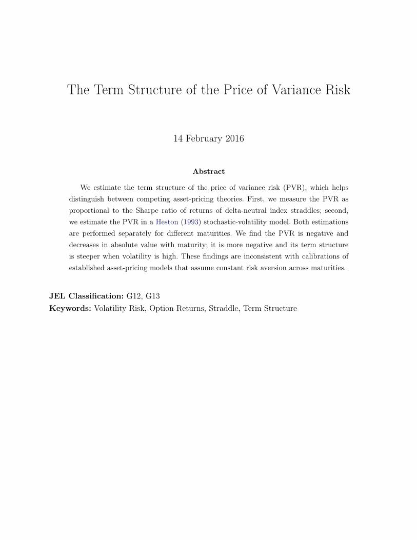
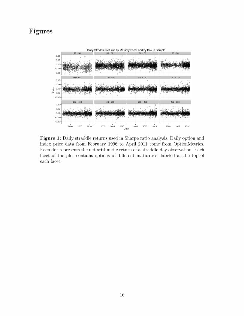
We estimate the Sharpe ratios of options with different maturities ranging from 11 days to252 days, using daily returns. To estimate the Sharpe ratio SRτ for options with maturity τ ,we use returns from options with maturities in the range [τ, τ + 20) and compute the averagedivided by the standard deviation of such returns. Figure 1 shows that these returns are notauto-correlated over time. Therefore, asymptotic standard errors for the Sharpe ratios canbe computed by bootstrapping, treating each return as an independent observation. Theresults of our analysis are described and discussed in Section 3.

2.3 Parametric Estimation Procedure

The factor√vt∆t/σ in Equation (6), while constant in the term-structure, may vary in

the time series. These time series variations can be correlated—and we show in Section 3that they are—with variations in the slope of the PVR term-structure. Such covariation canpotentially introduce a bias into the magnitude of the estimated slope in the Sharpe ratioanalysis described above. This concern motivates us to also estimate the parameter λ directlyin a parametric model, using a discrete-time method based on Christoffersen, Heston, andJacobs (2013, hereafter CHJ). CHJ estimate their model using a sample of options pooled

3Because the factor√vt∆t/σ is guaranteed to be positive, the Sharpe ratio is a robust test of the sign of

the PVR. Moreover, the extra factor√vt∆t/σ does not change with maturity, so it does not affect the sign

of the slope of the term structure of the PVR.

6

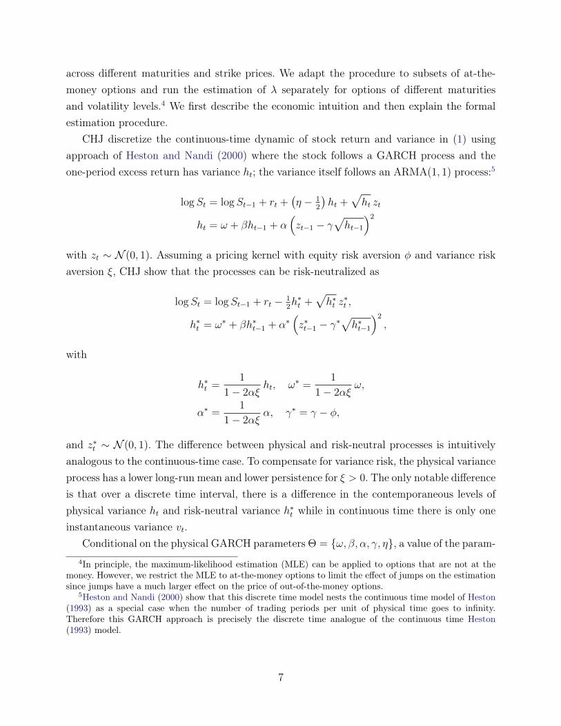
across different maturities and strike prices. We adapt the procedure to subsets of at-the-money options and run the estimation of λ separately for options of different maturitiesand volatility levels.4 We first describe the economic intuition and then explain the formalestimation procedure.

CHJ discretize the continuous-time dynamic of stock return and variance in (1) usingapproach of Heston and Nandi (2000) where the stock follows a GARCH process and theone-period excess return has variance ht; the variance itself follows an ARMA(1, 1) process:5

logSt = logSt−1 + rt +(η − 1

2

)ht +

√ht zt

ht = ω + βht−1 + α(zt−1 − γ

√ht−1

)2

with zt ∼ N (0, 1). Assuming a pricing kernel with equity risk aversion φ and variance riskaversion ξ, CHJ show that the processes can be risk-neutralized as

logSt = logSt−1 + rt − 12h∗t +

√h∗t z

∗t ,

h∗t = ω∗ + βh∗t−1 + α∗(z∗t−1 − γ∗

√h∗t−1

)2

,

with

h∗t =1

1− 2αξht, ω∗ =

1

1− 2αξω,

α∗ =1

1− 2αξα, γ∗ = γ − φ,

and z∗t ∼ N (0, 1). The difference between physical and risk-neutral processes is intuitivelyanalogous to the continuous-time case. To compensate for variance risk, the physical varianceprocess has a lower long-run mean and lower persistence for ξ > 0. The only notable differenceis that over a discrete time interval, there is a difference in the contemporaneous levels ofphysical variance ht and risk-neutral variance h∗t while in continuous time there is only oneinstantaneous variance vt.

Conditional on the physical GARCH parameters Θ = {ω, β, α, γ, η}, a value of the param-4In principle, the maximum-likelihood estimation (MLE) can be applied to options that are not at the

money. However, we restrict the MLE to at-the-money options to limit the effect of jumps on the estimationsince jumps have a much larger effect on the price of out-of-the-money options.

5Heston and Nandi (2000) show that this discrete time model nests the continuous time model of Heston(1993) as a special case when the number of trading periods per unit of physical time goes to infinity.Therefore this GARCH approach is precisely the discrete time analogue of the continuous time Heston(1993) model.

7

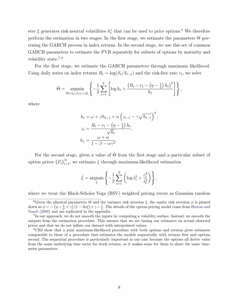
eter ξ generates risk-neutral volatilities h∗t that can be used to price options.6 We thereforeperform the estimation in two stages: In the first stage, we estimate the parameters Θ gov-erning the GARCH process in index returns. In the second stage, we use this set of commonGARCH parameters to estimate the PVR separately for subsets of options by maturity andvolatility state.7,8

For the first stage, we estimate the GARCH parameters through maximum likelihood.Using daily series on index returns Rt = log(St/St−1) and the risk-free rate rt, we solve

Θ = argminΘ={ω,β,α,γ,η}

{−1

2

T∑t=1

[log ht +

(Rt − rt −

(η − 1

2

)ht)2

ht

]},

where

ht = ω + βht−1 + α(zt−1 − γ

√ht−1

)2

,

zt =Rt − rt −

(η − 1

2

)ht√

ht,

h1 =ω + α

1− β − αγ2.

For the second stage, given a value of Θ from the first stage and a particular subset ofoption prices {Pi}Ni=1, we estimate ξ through maximum-likelihood estimation

ξ = argminξ

{−1

2

N∑i=1

(log s2

ε +ε2i

s2ε

)},

where we treat the Black-Scholes Vega (BSV) weighted pricing errors as Gaussian random6Given the physical parameters Θ and the variance risk aversion ξ, the equity risk aversion φ is pinned

down as φ = −(η − 1

2 + γ)

(1− 2αξ) +γ− 12 . The details of the option-pricing model come from Heston and

Nandi (2000) and are replicated in the appendix.7In our approach, we do not smooth the inputs by computing a volatility surface. Instead, we smooth the

outputs from the estimation procedure. This ensures that we are basing our estimates on actual observedprices and that we do not inflate our dataset with interpolated values.

8CHJ show that a joint maximum-likelihood procedure with both options and returns gives estimatescomparable to those of a procedure that estimates the models sequentially with returns first and optionssecond. The sequential procedure is particularly important in our case because the options all derive valuefrom the same underlying time series for stock returns, so it makes sense for them to share the same time-series parameters.

8

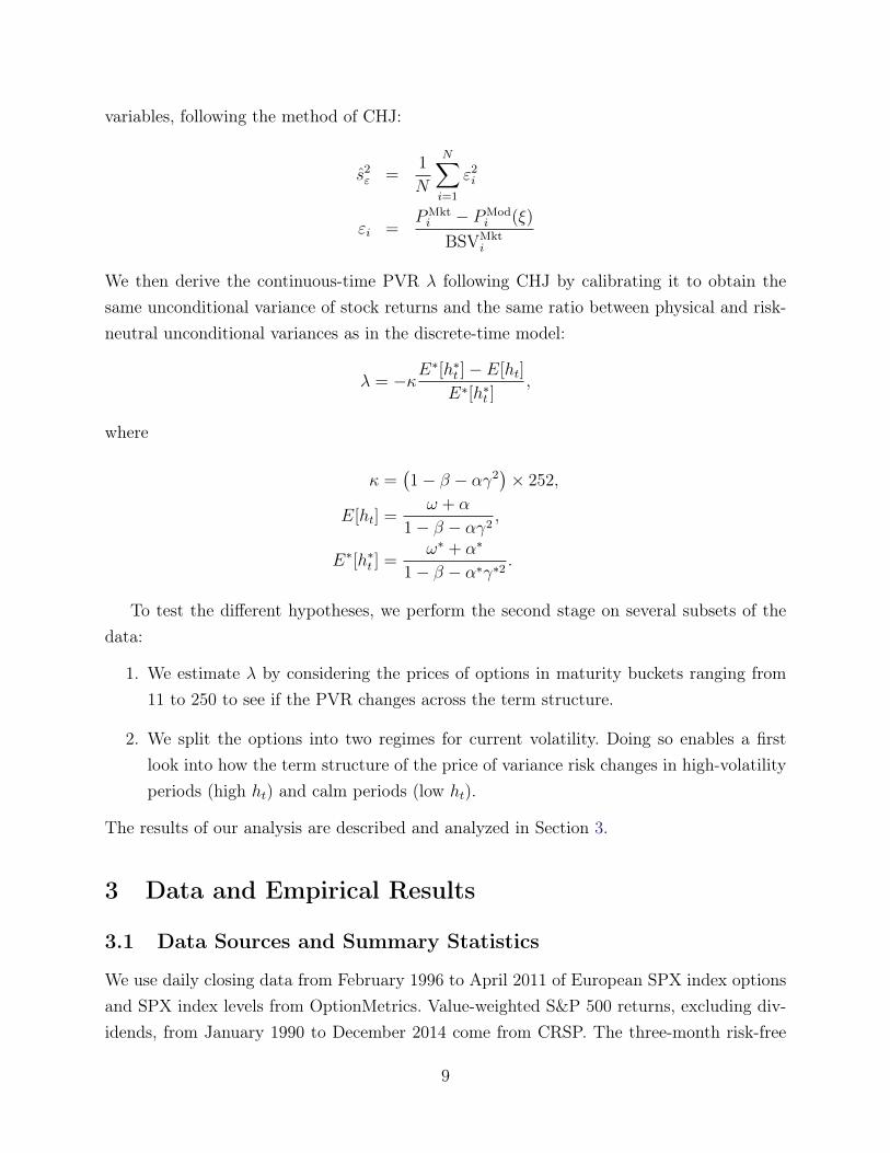
variables, following the method of CHJ:

s2ε =

1

N

N∑i=1

ε2i

εi =PMkti − PMod

i (ξ)

BSVMkti

We then derive the continuous-time PVR λ following CHJ by calibrating it to obtain thesame unconditional variance of stock returns and the same ratio between physical and risk-neutral unconditional variances as in the discrete-time model:

λ = −κE∗[h∗t ]− E[ht]

E∗[h∗t ],

where

κ =(1− β − αγ2

)× 252,

E[ht] =ω + α

1− β − αγ2,

E∗[h∗t ] =ω∗ + α∗

1− β − α∗γ∗2.

To test the different hypotheses, we perform the second stage on several subsets of thedata:

1. We estimate λ by considering the prices of options in maturity buckets ranging from11 to 250 to see if the PVR changes across the term structure.

2. We split the options into two regimes for current volatility. Doing so enables a firstlook into how the term structure of the price of variance risk changes in high-volatilityperiods (high ht) and calm periods (low ht).

The results of our analysis are described and analyzed in Section 3.

3 Data and Empirical Results

3.1 Data Sources and Summary Statistics

We use daily closing data from February 1996 to April 2011 of European SPX index optionsand SPX index levels from OptionMetrics. Value-weighted S&P 500 returns, excluding div-idends, from January 1990 to December 2014 come from CRSP. The three-month risk-free

9

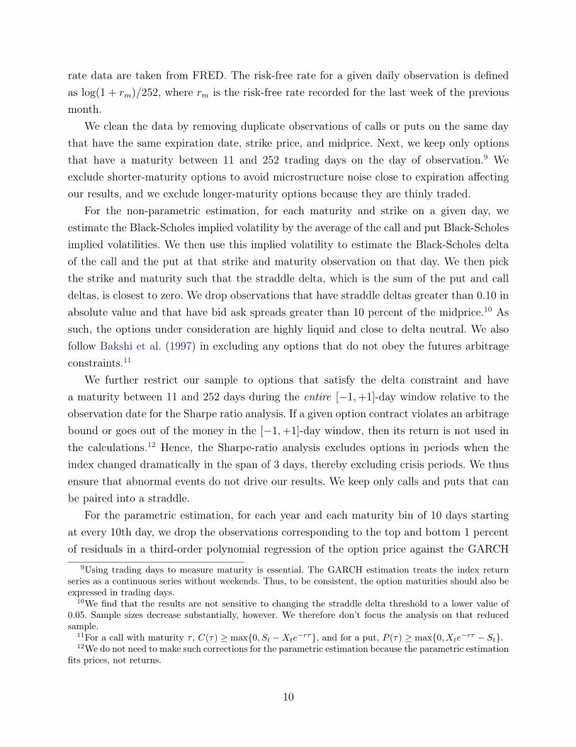
rate data are taken from FRED. The risk-free rate for a given daily observation is definedas log(1 + rm)/252, where rm is the risk-free rate recorded for the last week of the previousmonth.

We clean the data by removing duplicate observations of calls or puts on the same daythat have the same expiration date, strike price, and midprice. Next, we keep only optionsthat have a maturity between 11 and 252 trading days on the day of observation.9 Weexclude shorter-maturity options to avoid microstructure noise close to expiration affectingour results, and we exclude longer-maturity options because they are thinly traded.

For the non-parametric estimation, for each maturity and strike on a given day, weestimate the Black-Scholes implied volatility by the average of the call and put Black-Scholesimplied volatilities. We then use this implied volatility to estimate the Black-Scholes deltaof the call and the put at that strike and maturity observation on that day. We then pickthe strike and maturity such that the straddle delta, which is the sum of the put and calldeltas, is closest to zero. We drop observations that have straddle deltas greater than 0.10 inabsolute value and that have bid ask spreads greater than 10 percent of the midprice.10 Assuch, the options under consideration are highly liquid and close to delta neutral. We alsofollow Bakshi et al. (1997) in excluding any options that do not obey the futures arbitrageconstraints.11

We further restrict our sample to options that satisfy the delta constraint and havea maturity between 11 and 252 days during the entire [−1,+1]-day window relative to theobservation date for the Sharpe ratio analysis. If a given option contract violates an arbitragebound or goes out of the money in the [−1,+1]-day window, then its return is not used inthe calculations.12 Hence, the Sharpe-ratio analysis excludes options in periods when theindex changed dramatically in the span of 3 days, thereby excluding crisis periods. We thusensure that abnormal events do not drive our results. We keep only calls and puts that canbe paired into a straddle.

For the parametric estimation, for each year and each maturity bin of 10 days startingat every 10th day, we drop the observations corresponding to the top and bottom 1 percentof residuals in a third-order polynomial regression of the option price against the GARCH

9Using trading days to measure maturity is essential. The GARCH estimation treats the index returnseries as a continuous series without weekends. Thus, to be consistent, the option maturities should also beexpressed in trading days.

10We find that the results are not sensitive to changing the straddle delta threshold to a lower value of0.05. Sample sizes decrease substantially, however. We therefore don’t focus the analysis on that reducedsample.

11For a call with maturity τ , C(τ) ≥ max{0, St −Xte−rτ}, and for a put, P (τ) ≥ max{0, Xte

−rτ − St}.12We do not need to make such corrections for the parametric estimation because the parametric estimation

fits prices, not returns.

10

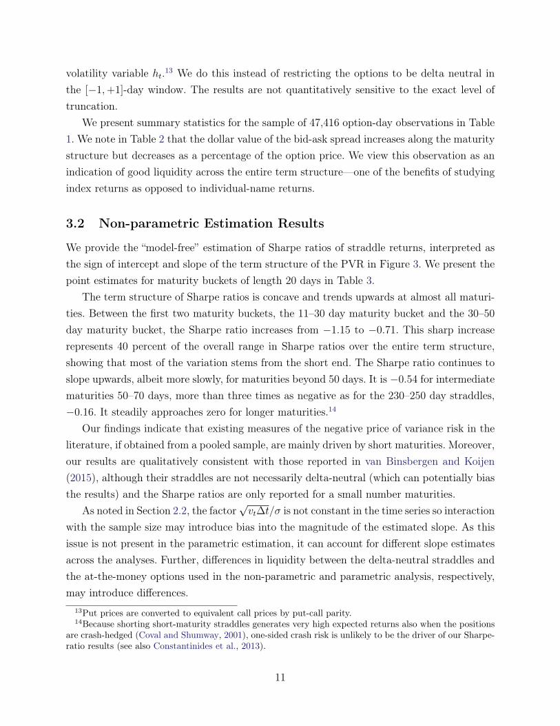
volatility variable ht.13 We do this instead of restricting the options to be delta neutral inthe [−1,+1]-day window. The results are not quantitatively sensitive to the exact level oftruncation.

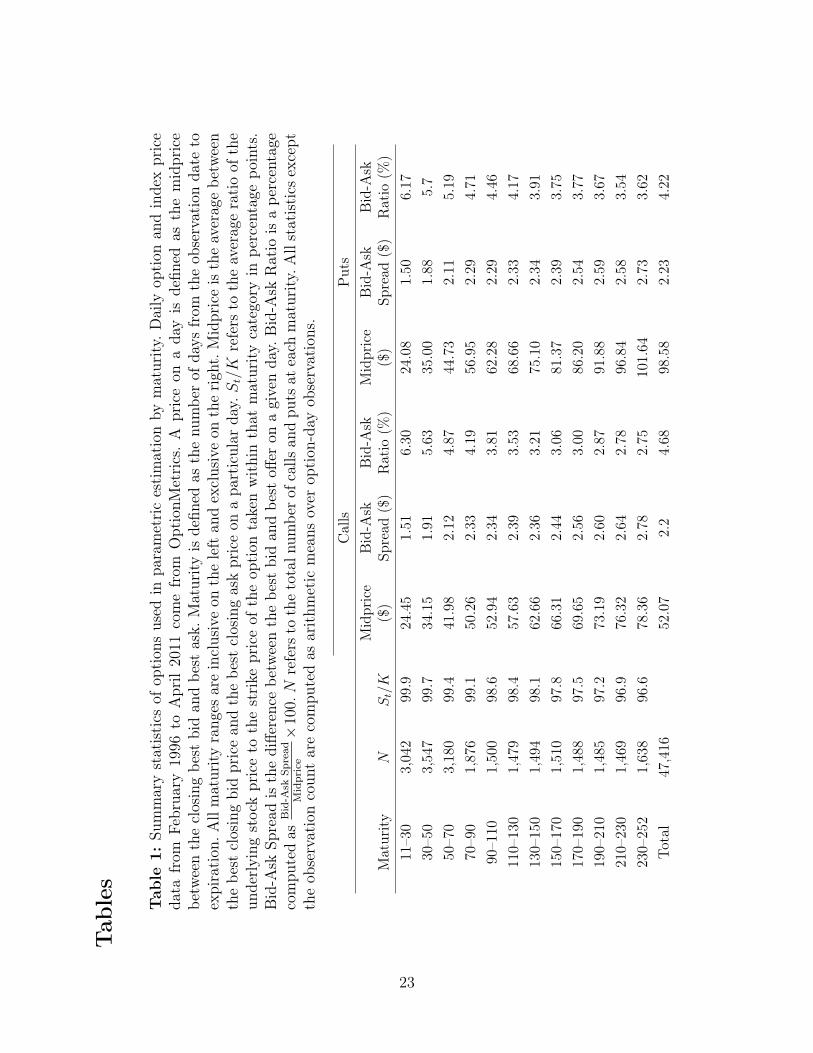
We present summary statistics for the sample of 47,416 option-day observations in Table1. We note in Table 2 that the dollar value of the bid-ask spread increases along the maturitystructure but decreases as a percentage of the option price. We view this observation as anindication of good liquidity across the entire term structure—one of the benefits of studyingindex returns as opposed to individual-name returns.

3.2 Non-parametric Estimation Results

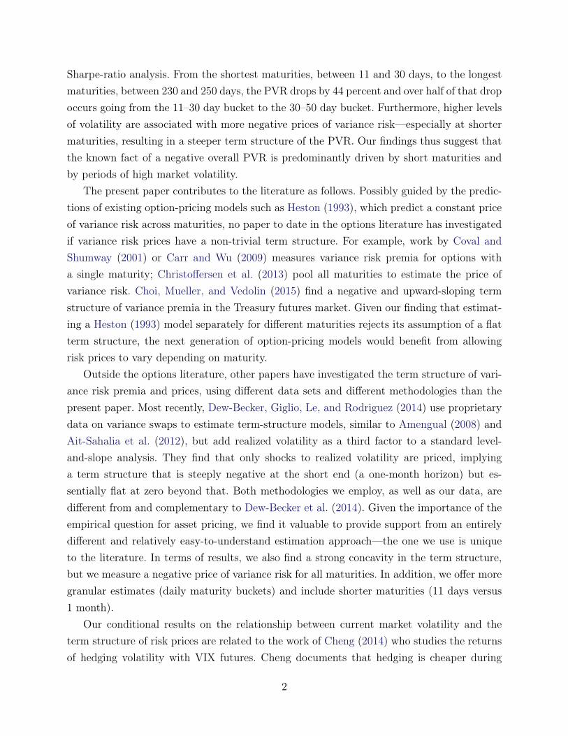
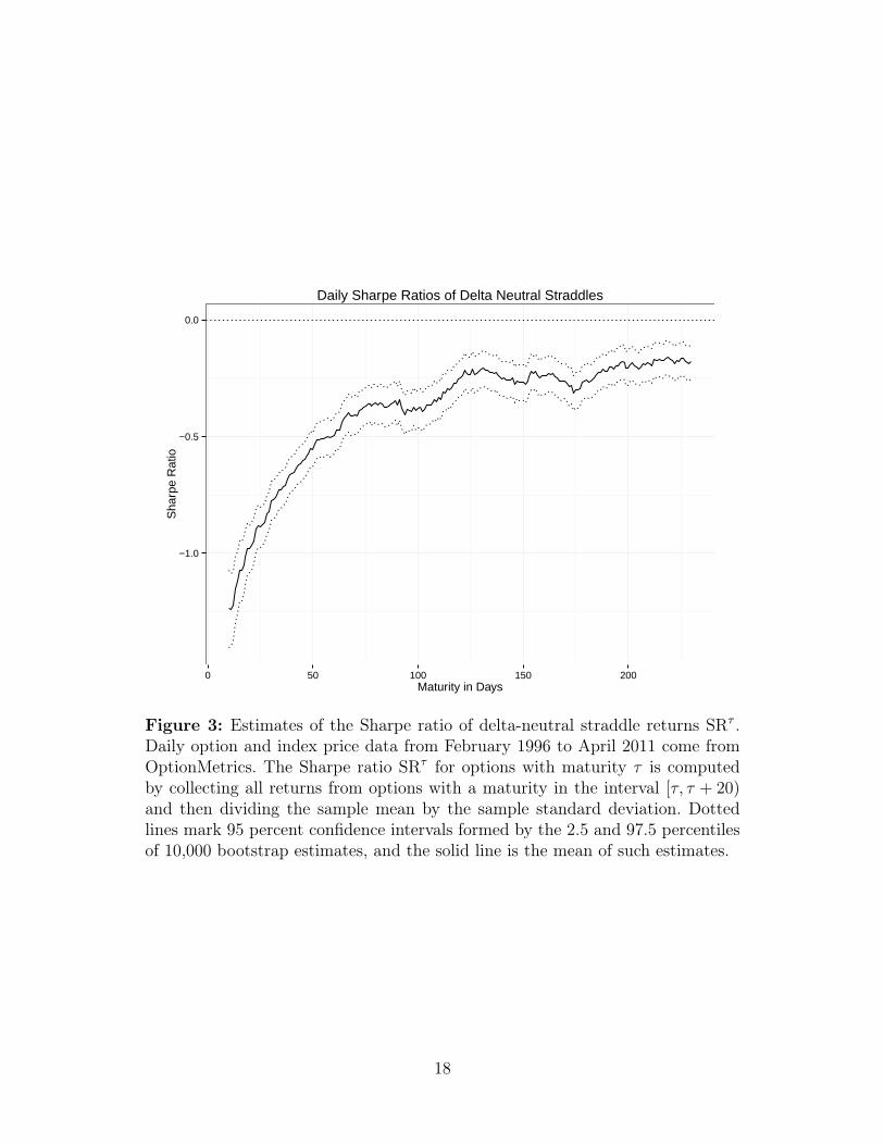
We provide the “model-free” estimation of Sharpe ratios of straddle returns, interpreted asthe sign of intercept and slope of the term structure of the PVR in Figure 3. We present thepoint estimates for maturity buckets of length 20 days in Table 3.

The term structure of Sharpe ratios is concave and trends upwards at almost all maturi-ties. Between the first two maturity buckets, the 11–30 day maturity bucket and the 30–50day maturity bucket, the Sharpe ratio increases from −1.15 to −0.71. This sharp increaserepresents 40 percent of the overall range in Sharpe ratios over the entire term structure,showing that most of the variation stems from the short end. The Sharpe ratio continues toslope upwards, albeit more slowly, for maturities beyond 50 days. It is −0.54 for intermediatematurities 50–70 days, more than three times as negative as for the 230–250 day straddles,−0.16. It steadily approaches zero for longer maturities.14

Our findings indicate that existing measures of the negative price of variance risk in theliterature, if obtained from a pooled sample, are mainly driven by short maturities. Moreover,our results are qualitatively consistent with those reported in van Binsbergen and Koijen(2015), although their straddles are not necessarily delta-neutral (which can potentially biasthe results) and the Sharpe ratios are only reported for a small number maturities.

As noted in Section 2.2, the factor√vt∆t/σ is not constant in the time series so interaction

with the sample size may introduce bias into the magnitude of the estimated slope. As thisissue is not present in the parametric estimation, it can account for different slope estimatesacross the analyses. Further, differences in liquidity between the delta-neutral straddles andthe at-the-money options used in the non-parametric and parametric analysis, respectively,may introduce differences.

13Put prices are converted to equivalent call prices by put-call parity.14Because shorting short-maturity straddles generates very high expected returns also when the positions

are crash-hedged (Coval and Shumway, 2001), one-sided crash risk is unlikely to be the driver of our Sharpe-ratio results (see also Constantinides et al., 2013).

11

3.3 Parametric Estimation Results

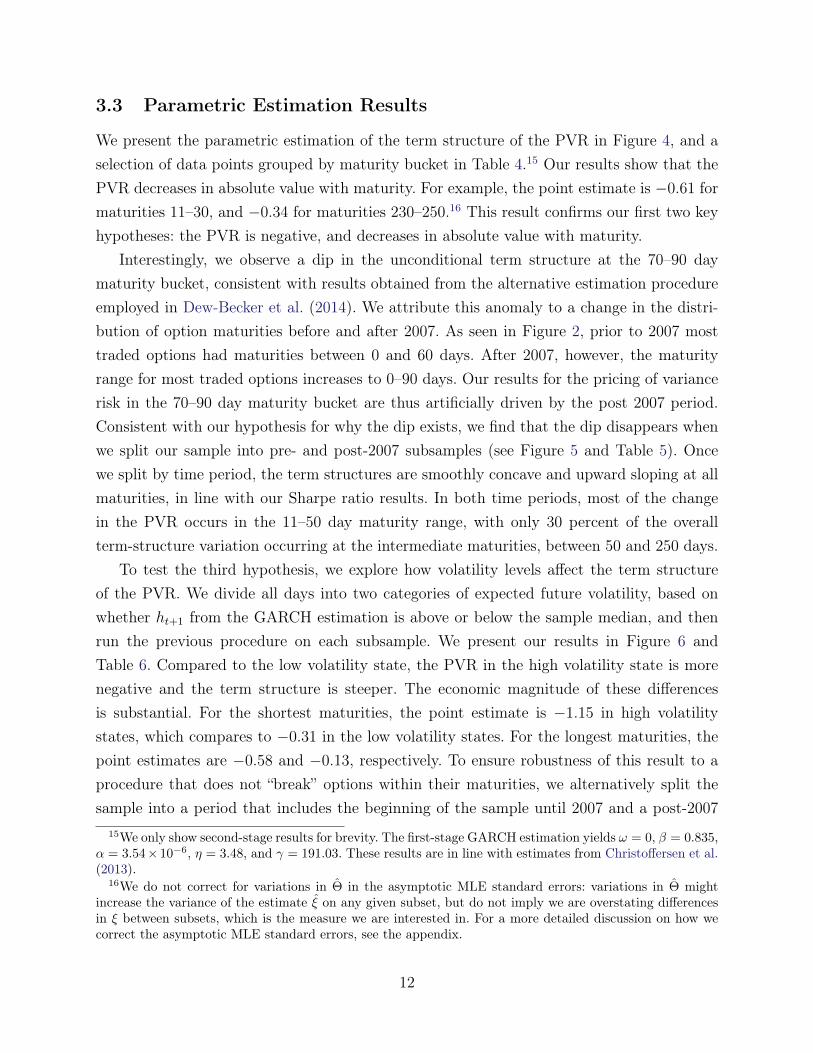
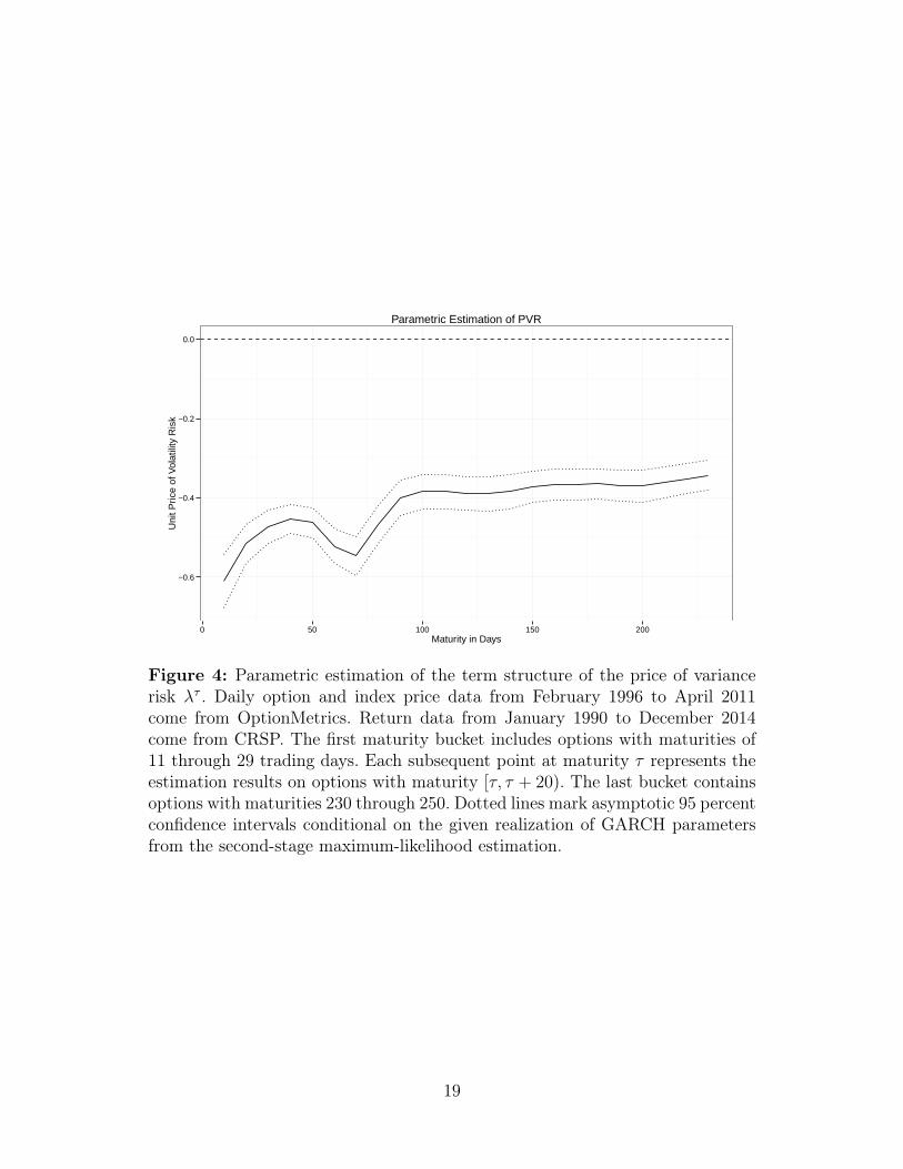
We present the parametric estimation of the term structure of the PVR in Figure 4, and aselection of data points grouped by maturity bucket in Table 4.15 Our results show that thePVR decreases in absolute value with maturity. For example, the point estimate is −0.61 formaturities 11–30, and −0.34 for maturities 230–250.16 This result confirms our first two keyhypotheses: the PVR is negative, and decreases in absolute value with maturity.

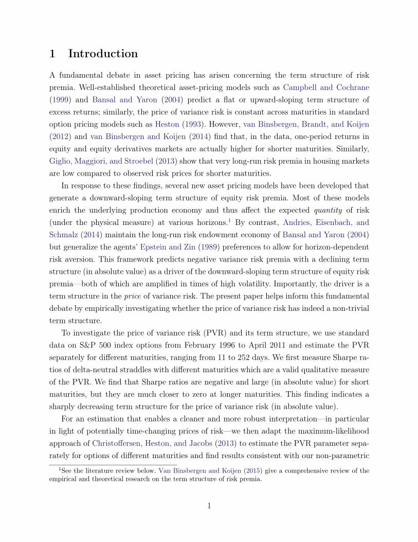
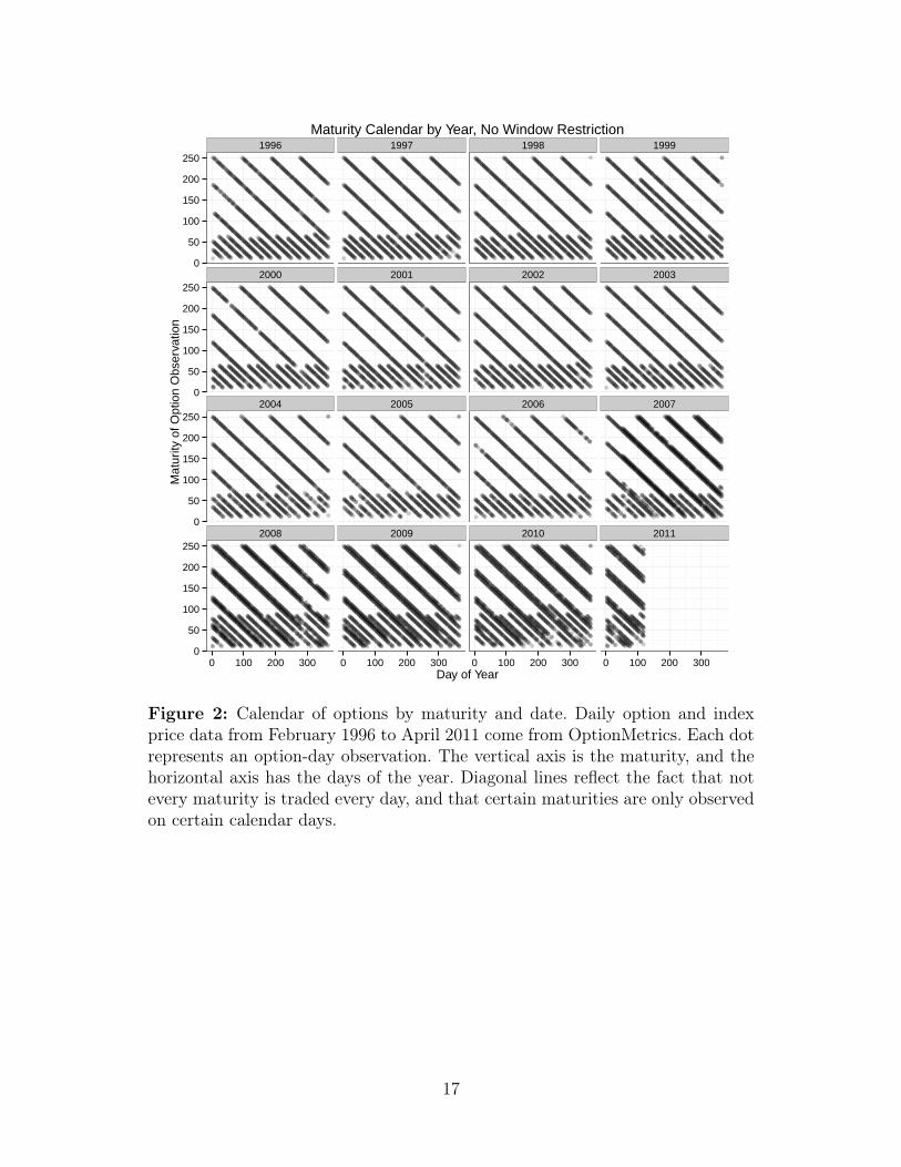
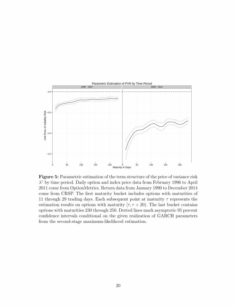
Interestingly, we observe a dip in the unconditional term structure at the 70–90 daymaturity bucket, consistent with results obtained from the alternative estimation procedureemployed in Dew-Becker et al. (2014). We attribute this anomaly to a change in the distri-bution of option maturities before and after 2007. As seen in Figure 2, prior to 2007 mosttraded options had maturities between 0 and 60 days. After 2007, however, the maturityrange for most traded options increases to 0–90 days. Our results for the pricing of variancerisk in the 70–90 day maturity bucket are thus artificially driven by the post 2007 period.Consistent with our hypothesis for why the dip exists, we find that the dip disappears whenwe split our sample into pre- and post-2007 subsamples (see Figure 5 and Table 5). Oncewe split by time period, the term structures are smoothly concave and upward sloping at allmaturities, in line with our Sharpe ratio results. In both time periods, most of the changein the PVR occurs in the 11–50 day maturity range, with only 30 percent of the overallterm-structure variation occurring at the intermediate maturities, between 50 and 250 days.

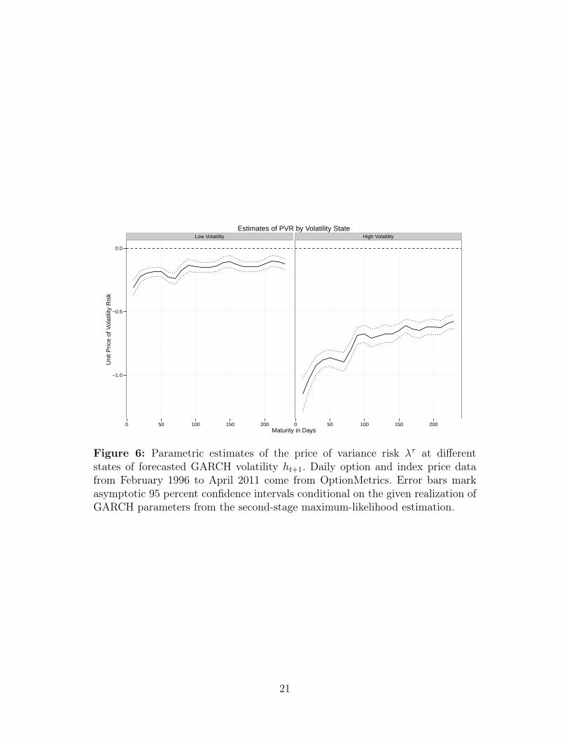
To test the third hypothesis, we explore how volatility levels affect the term structureof the PVR. We divide all days into two categories of expected future volatility, based onwhether ht+1 from the GARCH estimation is above or below the sample median, and thenrun the previous procedure on each subsample. We present our results in Figure 6 andTable 6. Compared to the low volatility state, the PVR in the high volatility state is morenegative and the term structure is steeper. The economic magnitude of these differencesis substantial. For the shortest maturities, the point estimate is −1.15 in high volatilitystates, which compares to −0.31 in the low volatility states. For the longest maturities, thepoint estimates are −0.58 and −0.13, respectively. To ensure robustness of this result to aprocedure that does not “break” options within their maturities, we alternatively split thesample into a period that includes the beginning of the sample until 2007 and a post-2007

15We only show second-stage results for brevity. The first-stage GARCH estimation yields ω = 0, β = 0.835,α = 3.54× 10−6, η = 3.48, and γ = 191.03. These results are in line with estimates from Christoffersen et al.(2013).

16We do not correct for variations in Θ in the asymptotic MLE standard errors: variations in Θ mightincrease the variance of the estimate ξ on any given subset, but do not imply we are overstating differencesin ξ between subsets, which is the measure we are interested in. For a more detailed discussion on how wecorrect the asymptotic MLE standard errors, see the appendix.

12

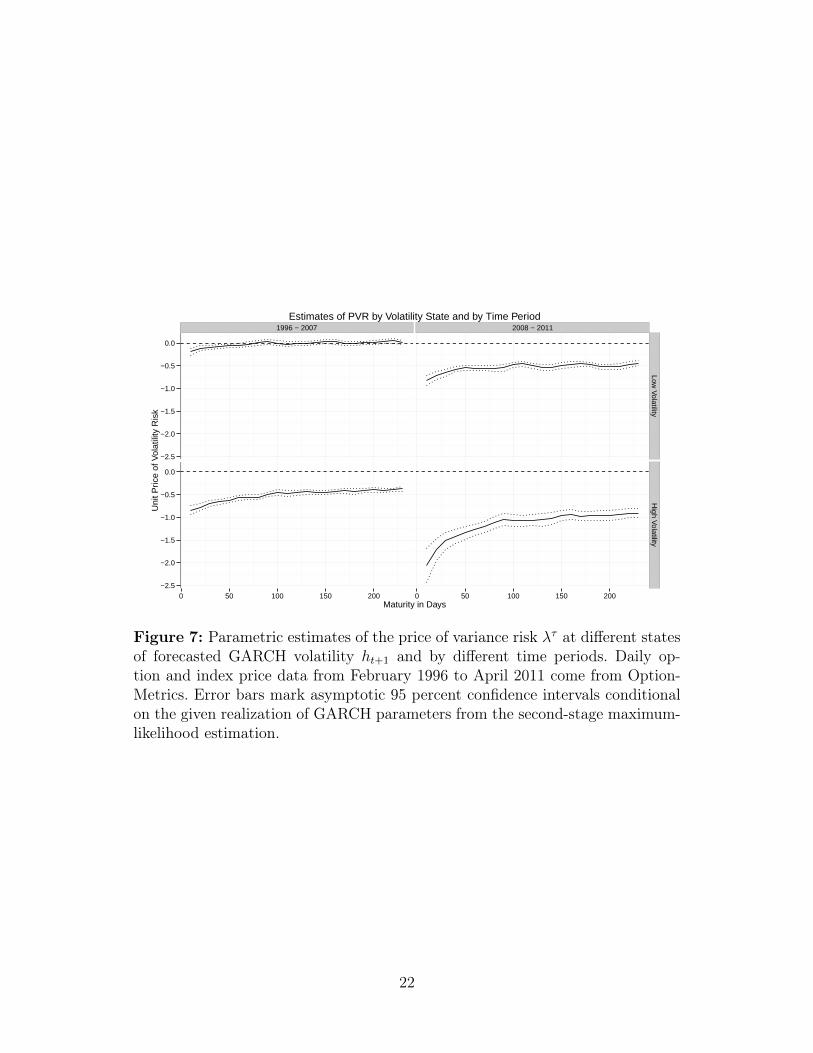
subsample, where the latter is a higher-volatility period. We find qualitatively similar results,presented in Figure 7 and Table 7. We conclude that the third hypothesis, a lower PVR andsteeper term structure, finds robust support in the data as well.

4 Conclusion

We provide estimates of the price of variance risk at various horizons, first, by measuringmodel-free Sharpe ratios of straddle returns with varying maturities and, second, by esti-mating the price of variance risk in a Heston (1993) model, based on the empirical approachdeveloped by Christoffersen et al. (2013). We find the price of insurance against increases involatilities varies with the horizon of the risk insured: short-term insurance is more expensivethan long-term insurance, and this effect is more pronounced in times of higher volatility.

These results extend the accumulating evidence for non-trivial term structures of riskprices to the market for variance risk. A comparative advantage to the literature is a focuson the price of risk as a driver of the term structure of risk premia. The findings thushelp motivate a new generation of option pricing models that allow for horizon-dependentrisk prices. However, our findings are informative not only for option pricing. Specifically,the results presented in this paper support preference-based rationalizations of the term-structure of expected returns, such as the horizon-dependent risk aversion model of Andrieset al. (2014).

The implicit assumption that risk prices are flat across horizons—which is rejected inthis paper—would lead market observers to attribute too much of the term structure ofrisk premia to a term structure in expected volatility. In other words, our results emphasizethat the conversion between objective and risk-neutral measures depends on maturity. Thisfinding may help inspire future generations of asset pricing models and econometricians’interpretation of economic forecasts.

13

References

Ait-Sahalia, Y., M. Karaman, and L. Mancini (2012). The term structure of variance swaps,risk premia, and the expectation hypothesis. Working Paper.

Amengual, D. (2008). The term structure of variance risk premia. Working Paper.

Andries, M. (2012). Consumption-based asset pricing with loss aversion. Working Paper.

Andries, M., T. M. Eisenbach, and M. C. Schmalz (2014). Asset pricing with horizon-dependent risk aversion. Working Paper.

Bakshi, G., C. Cao, and Z. Chen (1997, December). Empirical performance of alternativeoption pricing models. Journal of Finance 52 (5), 2003–2049.

Bansal, R., D. Kiku, I. Shaliastovich, and A. Yaron (2013). Volatility, the macroeconomy,and asset prices. Journal of Finance (forthcoming).

Bansal, R. and A. Yaron (2004). Risks for the long run: A potential resolution of assetpricing puzzles. Journal of Finance 59 (4), 1481–1509.

Barras, L. and A. Malkhozov (2015). Does variance risk have two prices? Evidence from theequity and option markets. Working Paper.

van Binsbergen, J., M. Brandt, and R. Koijen (2012). On the timing and pricing of dividends.American Economic Review 102 (4), 1596–1618.

van Binsbergen, J. and R. Koijen (2014). Real excess volatility. Working Paper.

van Binsbergen, J. and R. Koijen (2015). The term structure of returns: Facts and theory.Working Paper.

Campbell, J. Y. and J. H. Cochrane (1999). By force of habit: A consumption-based expla-nation of aggregate stock market behavior. Journal of Political Economy 107 (2), 205–251.

Carr, P. and L. Wu (2009). Variance risk premiums. Review of Financial Studies 22 (3),1311–1341.

Cheng, I.-H. (2014). The returns to fear. Working Paper.

Choi, H., P. Mueller, and A. Vedolin (2015). Bond variance risk premiums. Working Paper.

14

Christoffersen, P., S. Heston, and K. Jacobs (2013). Capturing option anomalies with avariance-dependent pricing kernel. Review of Financial Studies 26 (8), 1962–2006.

Constantinides, G. M., J. C. Jackwerth, and A. Savov (2013). The puzzle of index optionreturns. Review of Asset Pricing Studies 3 (2), 229–257.

Coval, J. D. and T. Shumway (2001). Expected option returns. Journal of Finance 56 (3),983–1009.

Curatola, G. (2014). Loss aversion, habit formation and the term structures of equity andinterest rates. Working Paper.

Dew-Becker, I., S. Giglio, A. Le, and M. Rodriguez (2014). The price of variance risk.Working Paper.

Epstein, L. G. and S. E. Zin (1989). Substitution, risk aversion, and the temporal behaviorof consumption and asset returns: A theoretical framework. Econometrica, 937–969.

Giglio, S., M. Maggiori, and J. Stroebel (2013). Very long-run discount rates. WorkingPaper.

Heston, S. (1993). A closed-form solution for options with stochastic volatility with appli-cations to bond and currency options. Review of Financial Studies 6 (2), 327–343.

Heston, S. and S. Nandi (2000). A closed-form GARCH option valuation model. Review ofFinancial Studies 13 (3), 585–625.

Wachter, J. A. (2013, June). Can time-varying risk of rare disasters explain aggregate stockmarket volatility? Journal of Finance 52 (3), 987–1035.

15

Figures

11 − 30 30 − 50 50 − 70 70 − 90

90 − 110 110 − 130 130 − 150 150 − 170

170 − 190 190 − 210 210 − 230 230 − 250

−0.10

−0.05

0.00

0.05

0.10

−0.10

−0.05

0.00

0.05

0.10

−0.10

−0.05

0.00

0.05

0.10

2000 2005 2010 2000 2005 2010 2000 2005 2010 2000 2005 2010Date

Ret

urn

Daily Straddle Returns by Maturity Facet and by Day in Sample

Figure 1: Daily straddle returns used in Sharpe ratio analysis. Daily option andindex price data from February 1996 to April 2011 come from OptionMetrics.Each dot represents the net arithmetic return of a straddle-day observation. Eachfacet of the plot contains options of different maturities, labeled at the top ofeach facet.

16

1996 1997 1998 1999

2000 2001 2002 2003

2004 2005 2006 2007

2008 2009 2010 2011

0

50

100

150

200

250

0

50

100

150

200

250

0

50

100

150

200

250

0

50

100

150

200

250

0 100 200 300 0 100 200 300 0 100 200 300 0 100 200 300Day of Year

Mat

urity

of O

ptio

n O

bser

vatio

n

Maturity Calendar by Year, No Window Restriction

Figure 2: Calendar of options by maturity and date. Daily option and indexprice data from February 1996 to April 2011 come from OptionMetrics. Each dotrepresents an option-day observation. The vertical axis is the maturity, and thehorizontal axis has the days of the year. Diagonal lines reflect the fact that notevery maturity is traded every day, and that certain maturities are only observedon certain calendar days.

17

−1.0

−0.5

0.0

0 50 100 150 200Maturity in Days

Sha

rpe

Rat

io

Daily Sharpe Ratios of Delta Neutral Straddles

Figure 3: Estimates of the Sharpe ratio of delta-neutral straddle returns SRτ .Daily option and index price data from February 1996 to April 2011 come fromOptionMetrics. The Sharpe ratio SRτ for options with maturity τ is computedby collecting all returns from options with a maturity in the interval [τ, τ + 20)and then dividing the sample mean by the sample standard deviation. Dottedlines mark 95 percent confidence intervals formed by the 2.5 and 97.5 percentilesof 10,000 bootstrap estimates, and the solid line is the mean of such estimates.

18

−0.6

−0.4

−0.2

0.0

0 50 100 150 200Maturity in Days

Uni

t Pric

e of

Vol

atili

ty R

isk

Parametric Estimation of PVR

Figure 4: Parametric estimation of the term structure of the price of variancerisk λτ . Daily option and index price data from February 1996 to April 2011come from OptionMetrics. Return data from January 1990 to December 2014come from CRSP. The first maturity bucket includes options with maturities of11 through 29 trading days. Each subsequent point at maturity τ represents theestimation results on options with maturity [τ, τ + 20). The last bucket containsoptions with maturities 230 through 250. Dotted lines mark asymptotic 95 percentconfidence intervals conditional on the given realization of GARCH parametersfrom the second-stage maximum-likelihood estimation.

19

1996 − 2007 2008 − 2011

−1.5

−1.0

−0.5

0.0

0 50 100 150 200 0 50 100 150 200Maturity in Days

Uni

t Pric

e of

Vol

atili

ty R

isk

Parametric Estimation of PVR by Time Period

Figure 5: Parametric estimation of the term structure of the price of variance riskλτ by time period. Daily option and index price data from February 1996 to April2011 come from OptionMetrics. Return data from January 1990 to December 2014come from CRSP. The first maturity bucket includes options with maturities of11 through 29 trading days. Each subsequent point at maturity τ represents theestimation results on options with maturity [τ, τ + 20). The last bucket containsoptions with maturities 230 through 250. Dotted lines mark asymptotic 95 percentconfidence intervals conditional on the given realization of GARCH parametersfrom the second-stage maximum-likelihood estimation.

20

Low Volatility High Volatility

−1.0

−0.5

0.0

0 50 100 150 200 0 50 100 150 200Maturity in Days

Uni

t Pric

e of

Vol

atili

ty R

isk

Estimates of PVR by Volatility State

Figure 6: Parametric estimates of the price of variance risk λτ at differentstates of forecasted GARCH volatility ht+1. Daily option and index price datafrom February 1996 to April 2011 come from OptionMetrics. Error bars markasymptotic 95 percent confidence intervals conditional on the given realization ofGARCH parameters from the second-stage maximum-likelihood estimation.

21

1996 − 2007 2008 − 2011

−2.5

−2.0

−1.5

−1.0

−0.5

0.0

−2.5

−2.0

−1.5

−1.0

−0.5

0.0

Low V

olatilityH

igh Volatility

0 50 100 150 200 0 50 100 150 200Maturity in Days

Uni

t Pric

e of

Vol

atili

ty R

isk

Estimates of PVR by Volatility State and by Time Period

Figure 7: Parametric estimates of the price of variance risk λτ at different statesof forecasted GARCH volatility ht+1 and by different time periods. Daily op-tion and index price data from February 1996 to April 2011 come from Option-Metrics. Error bars mark asymptotic 95 percent confidence intervals conditionalon the given realization of GARCH parameters from the second-stage maximum-likelihood estimation.

22

Tab

les

Tab

le1:

Summarystatistics

ofop

tion

sused

inpa

rametricestimationby

maturity

.Daily

option

andindexprice

data

from

Februa

ry19

96to

April20

11comefrom

OptionM

etrics.A

priceon

ada

yis

defin

edas

themidprice

betw

eentheclosingbe

stbidan

dbe

stask.

Maturity

isdefin

edas

thenu

mbe

rof

days

from

theob

servationda

teto

expiration

.Allmaturity

rang

esareinclusiveon

theleftan

dexclusiveon

therigh

t.Midpriceistheaverag

ebe

tween

thebe

stclosingbidpricean

dthebe

stclosingaskpriceon

apa

rticular

day.St/K

refers

totheaverag

eratioof

the

underlying

stockpriceto

thestrike

priceof

theop

tion

takenwithinthat

maturity

catego

ryin

percentage

points.

Bid-A

skSp

read

isthediffe

rencebe

tweenthebe

stbidan

dbe

stoff

eron

agivenda

y.Bid-A

skRatio

isape

rcentage

compu

tedas

Bid

-Ask

Spre

adM

idpr

ice×

100.N

refers

tothetotaln

umbe

rof

calls

andpu

tsat

each

maturity

.Allstatistics

except

theob

servationcoun

tarecompu

tedas

arithm

etic

means

over

option

-day

observations.

Calls

Puts

Maturity

NSt/K

Midprice

($)

Bid-A

skSp

read

($)

Bid-A

skRatio

(%)

Midprice

($)

Bid-A

skSp

read

($)

Bid-A

skRatio

(%)

11–30

3,042

99.9

24.45

1.51

6.30

24.08

1.50

6.17

30–50

3,547

99.7

34.15

1.91

5.63

35.00

1.88

5.7

50–70

3,180

99.4

41.98

2.12

4.87

44.73

2.11

5.19

70–90

1,876

99.1

50.26

2.33

4.19

56.95

2.29

4.71

90–110

1,500

98.6

52.94

2.34

3.81

62.28

2.29

4.46

110–130

1,479

98.4

57.63

2.39

3.53

68.66

2.33

4.17

130–150

1,494

98.1

62.66

2.36

3.21

75.10

2.34

3.91

150–170

1,510

97.8

66.31

2.44

3.06

81.37

2.39

3.75

170–190

1,488

97.5

69.65

2.56

3.00

86.20

2.54

3.77

190–210

1,485

97.2

73.19

2.60

2.87

91.88

2.59

3.67

210–230

1,469

96.9

76.32

2.64

2.78

96.84

2.58

3.54

230–252

1,638

96.6

78.36

2.78

2.75

101.64

2.73

3.62

Total

47,416

52.07

2.2

4.68

98.58

2.23

4.22

23

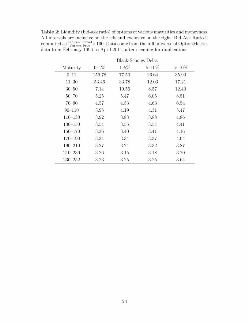
Table 2: Liquidity (bid-ask ratio) of options of various maturities and moneyness.All intervals are inclusive on the left and exclusive on the right. Bid-Ask Ratio iscomputed as Bid-Ask Spread

Current Price ×100. Data come from the full universe of OptionMetricsdata from February 1996 to April 2011, after cleaning for duplications.

Black-Scholes DeltaMaturity 0–1% 1–5% 5–10% > 10%0–11 159.78 77.50 26.64 35.9011–30 53.46 33.78 12.03 17.2130–50 7.14 10.56 8.57 12.4050–70 5.25 5.47 6.05 8.5170–90 4.57 4.53 4.63 6.5490–110 3.95 4.19 4.31 5.47110–130 3.92 3.83 3.88 4.86130–150 3.54 3.55 3.54 4.41150–170 3.36 3.40 3.41 4.16170–190 3.34 3.34 3.37 4.04190–210 3.27 3.24 3.32 3.87210–230 3.26 3.15 3.18 3.70230–252 3.23 3.25 3.25 3.64

24

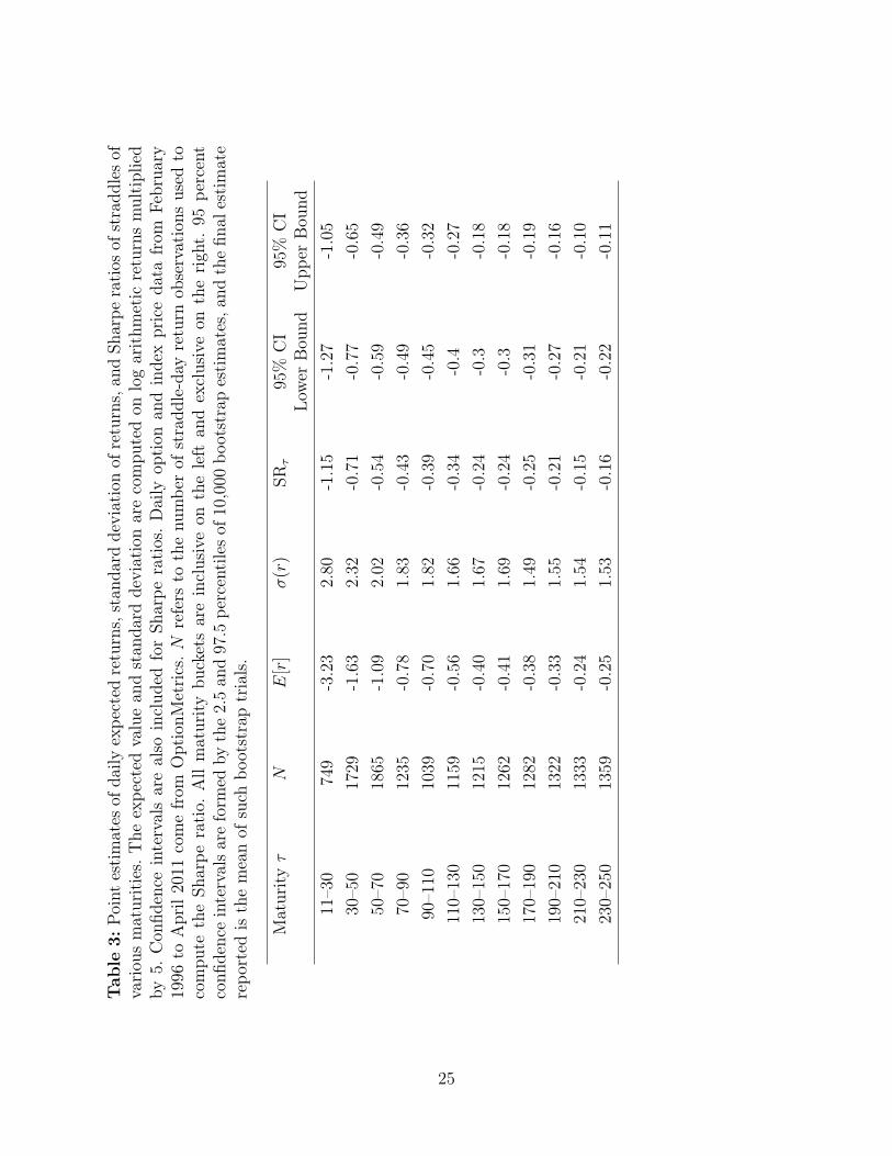
Tab

le3:

Point

estimates

ofda

ilyexpe

cted

returns,stan

dard

deviationof

returns,an

dSh

arpe

ratios

ofstradd

lesof

variou

smaturities.

The

expe

cted

valuean

dstan

dard

deviationarecompu

tedon

logarithm

etic

returnsmultiplied

by5.

Con

fidence

intervalsarealso

includ

edforSh

arpe

ratios.Daily

option

andindexpriceda

tafrom

Februa

ry19

96to

April20

11comefrom

OptionM

etrics.N

refers

tothenu

mbe

rof

stradd

le-day

return

observations

used

tocompu

tetheSh

arpe

ratio.

Allmaturity

bucketsareinclusiveon

theleft

andexclusiveon

therigh

t.95

percent

confi

denceintervalsareform

edby

the2.5an

d97

.5pe

rcentilesof

10,000

bootstrapestimates,a

ndthefin

alestimate

repo

rted

isthemeanof

such

bootstraptrials.

Maturity

τN

E[r

]σ

(r)

SRτ

95%

CI

Lower

Bou

nd95

%CI

Upp

erBou

nd11

–30

749

-3.23

2.80

-1.15

-1.27

-1.05

30–5

017

29-1.63

2.32

-0.71

-0.77

-0.65

50–7

018

65-1.09

2.02

-0.54

-0.59

-0.49

70–9

012

35-0.78

1.83

-0.43

-0.49

-0.36

90–1

1010

39-0.70

1.82

-0.39

-0.45

-0.32

110–

130

1159

-0.56

1.66

-0.34

-0.4

-0.27

130–

150

1215

-0.40

1.67

-0.24

-0.3

-0.18

150–

170

1262

-0.41

1.69

-0.24

-0.3

-0.18

170–

190

1282

-0.38

1.49

-0.25

-0.31

-0.19

190–

210

1322

-0.33

1.55

-0.21

-0.27

-0.16

210–

230

1333

-0.24

1.54

-0.15

-0.21

-0.10

230–

250

1359

-0.25

1.53

-0.16

-0.22

-0.11

25

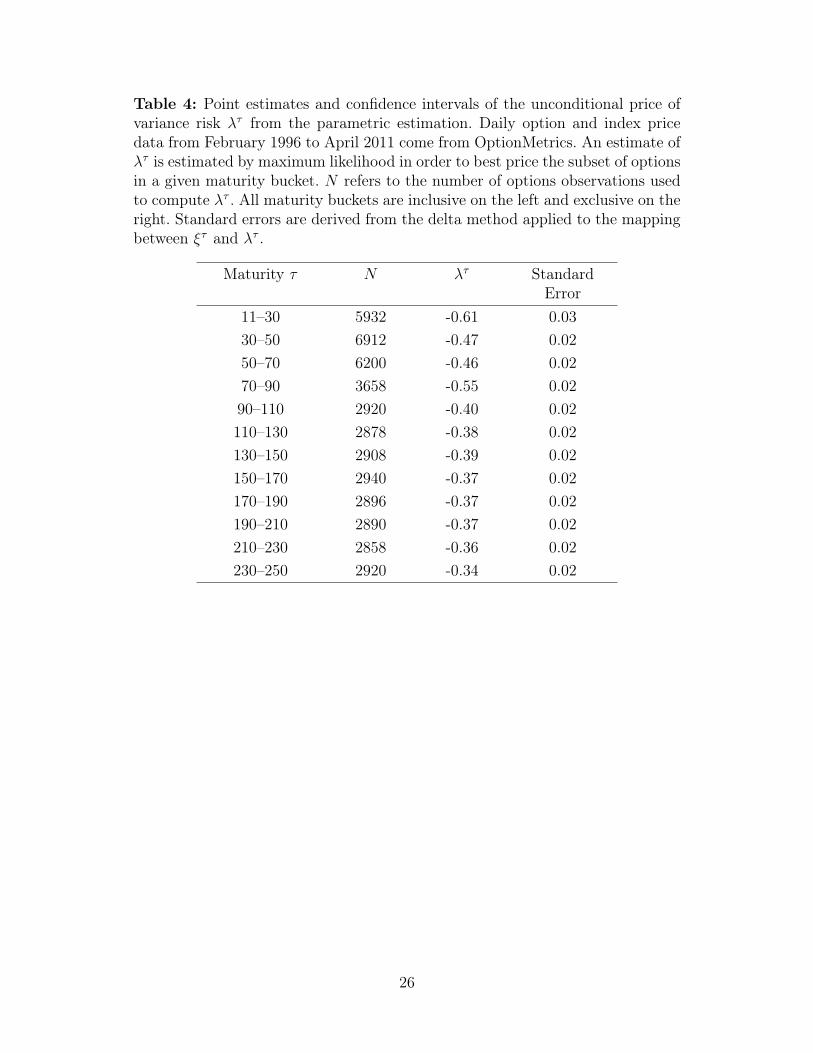
Table 4: Point estimates and confidence intervals of the unconditional price ofvariance risk λτ from the parametric estimation. Daily option and index pricedata from February 1996 to April 2011 come from OptionMetrics. An estimate ofλτ is estimated by maximum likelihood in order to best price the subset of optionsin a given maturity bucket. N refers to the number of options observations usedto compute λτ . All maturity buckets are inclusive on the left and exclusive on theright. Standard errors are derived from the delta method applied to the mappingbetween ξτ and λτ .

Maturity τ N λτ StandardError

11–30 5932 -0.61 0.0330–50 6912 -0.47 0.0250–70 6200 -0.46 0.0270–90 3658 -0.55 0.0290–110 2920 -0.40 0.02110–130 2878 -0.38 0.02130–150 2908 -0.39 0.02150–170 2940 -0.37 0.02170–190 2896 -0.37 0.02190–210 2890 -0.37 0.02210–230 2858 -0.36 0.02230–250 2920 -0.34 0.02

26

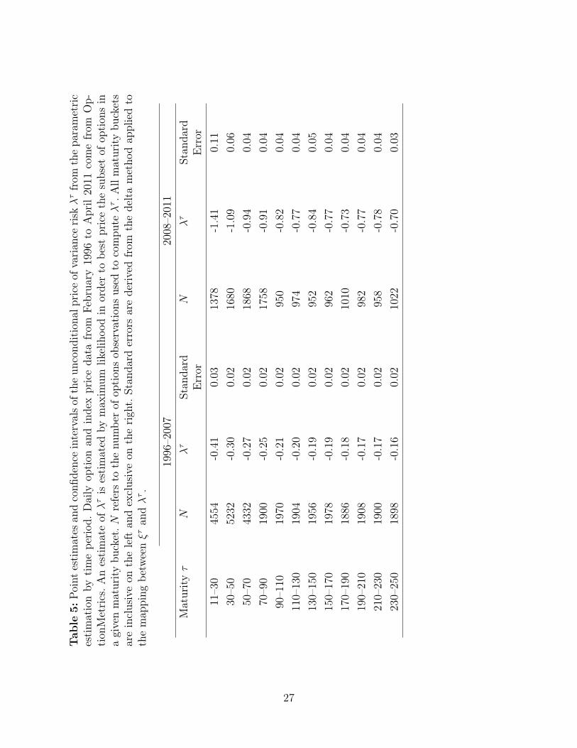
Tab

le5:

Point

estimates

andconfi

denceintervalsof

theun

cond

itiona

lprice

ofvarian

ceriskλτfrom

thepa

rametric

estimationby

timepe

riod

.Daily

option

andindexpriceda

tafrom

Februa

ry19

96to

April20

11comefrom

Op-

tion

Metrics.A

nestimateofλτis

estimated

bymax

imum

likelihoo

din

orderto

best

pricethesubset

ofop

tion

sin

agivenmaturity

bucket.N

refers

tothenu

mbe

rof

option

sob

servations

used

tocompu

teλτ.A

llmaturity

buckets

areinclusiveon

theleft

andexclusiveon

therigh

t.Stan

dard

errors

arederivedfrom

thedeltametho

dap

pliedto

themap

ping

betw

eenξτ

andλτ.

1996

–200

720

08–2

011

Maturity

τN

λτ

Stan

dard

Error

Nλτ

Stan

dard

Error

11–3

045

54-0.41

0.03

1378

-1.41

0.11

30–5

052

32-0.30

0.02

1680

-1.09

0.06

50–7

043

32-0.27

0.02

1868

-0.94

0.04

70–9

019

00-0.25

0.02

1758

-0.91

0.04

90–1

1019

70-0.21

0.02

950

-0.82

0.04

110–

130

1904

-0.20

0.02

974

-0.77

0.04

130–

150

1956

-0.19

0.02

952

-0.84

0.05

150–

170

1978

-0.19

0.02

962

-0.77

0.04

170–

190

1886

-0.18

0.02

1010

-0.73

0.04

190–

210

1908

-0.17

0.02

982

-0.77

0.04

210–

230

1900

-0.17

0.02

958

-0.78

0.04

230–

250

1898

-0.16

0.02

1022

-0.70

0.03

27

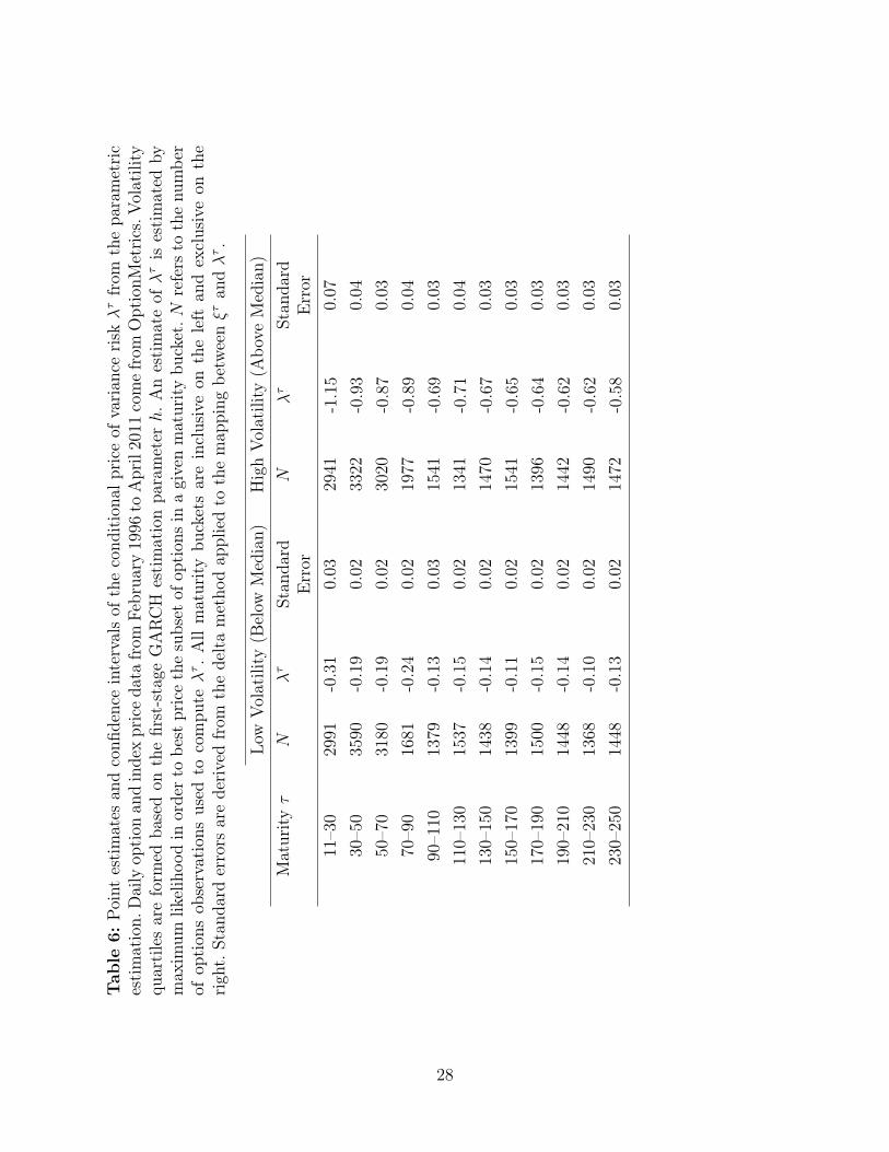
Tab

le6:

Point

estimates

andconfi

denc

eintervalsof

thecond

itiona

lprice

ofvarian

ceriskλτfrom

thepa

rametric

estimation.

Daily

option

andindexpriceda

tafrom

Februa

ry19

96to

April20

11comefrom

OptionM

etrics.V

olatility

quartilesareform

edba

sedon

thefirst-stage

GARCH

estimationpa

rameterh.Anestimateofλτis

estimated

bymax

imum

likelihoo

din

orderto

best

pricethesubset

ofop

tion

sin

agivenmaturity

bucket.N

refers

tothenu

mbe

rof

option

sob

servations

used

tocompu

teλτ.Allmaturity

bucketsareinclusiveon

theleft

andexclusiveon

the

righ

t.Stan

dard

errors

arederivedfrom

thedeltametho

dap

pliedto

themap

ping

betw

eenξτ

andλτ.

Low

Volatility

(Below

Median)

HighVolatility

(Abo

veMedian)

Maturity

τN

λτ

Stan

dard

Error

Nλτ

Stan

dard

Error

11–3

029

91-0.31

0.03

2941

-1.15

0.07

30–5

035

90-0.19

0.02

3322

-0.93

0.04

50–7

031

80-0.19

0.02

3020

-0.87

0.03

70–9

016

81-0.24

0.02

1977

-0.89

0.04

90–1

1013

79-0.13

0.03

1541

-0.69

0.03

110–

130

1537

-0.15

0.02

1341

-0.71

0.04

130–

150

1438

-0.14

0.02

1470

-0.67

0.03

150–

170

1399

-0.11

0.02

1541

-0.65

0.03

170–

190

1500

-0.15

0.02

1396

-0.64

0.03

190–

210

1448

-0.14

0.02

1442

-0.62

0.03

210–

230

1368

-0.10

0.02

1490

-0.62

0.03

230–

250

1448

-0.13

0.02

1472

-0.58

0.03

28

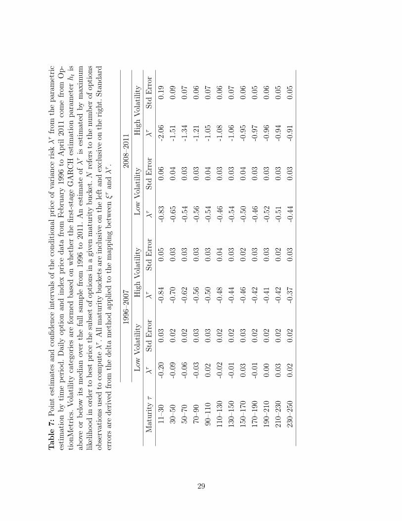
Tab

le7:

Point

estimates

andconfi

denc

eintervalsof

thecond

itiona

lprice

ofvarian

ceriskλτfrom

thepa

rametric

estimationby

timepe

riod

.Daily

option

andindexpriceda

tafrom

Februa

ry19

96to

April20

11comefrom

Op-

tion

Metrics.V

olatility

categories

areform

edba

sedon

whether

thefirst-stage

GARCH

estimationpa

rameterhtis

aboveor

below

itsmedianover

thefullsamplefrom

1996

to20

11.Anestimateofλτis

estimated

bymax

imum

likelihoo

din

orderto

best

pricethesubset

ofop

tion

sin

agivenmaturity

bucket.N

refers

tothenu

mbe

rof

option

sob

servations

used

tocompu

teλτ.A

llmaturity

bucketsareinclusiveon

theleftan

dexclusiveon

therigh

t.Stan

dard

errors

arederivedfrom

thedeltametho

dap

pliedto

themap

ping

betw

eenξτ

andλτ.

1996

–200

720

08–2

011

Low

Volatility

HighVolatility

Low

Volatility

HighVolatility

Maturity

τλτ

StdError

λτ

StdError

λτ

StdError

λτ

StdError

11–3

0-0.20

0.03

-0.84

0.05

-0.83

0.06

-2.06

0.19

30–5

0-0.09

0.02

-0.70

0.03

-0.65

0.04

-1.51

0.09

50–7

0-0.06

0.02

-0.62

0.03

-0.54

0.03

-1.34

0.07

70–9

0-0.03

0.03

-0.56

0.03

-0.56

0.03

-1.21

0.06

90–1

100.02

0.03

-0.50

0.03

-0.54

0.04

-1.05

0.07

110–

130

-0.02

0.02

-0.48

0.04

-0.46

0.03

-1.08

0.06

130–

150

-0.01

0.02

-0.44

0.03

-0.54

0.03

-1.06

0.07

150–

170

0.03

0.03

-0.46

0.02

-0.50

0.04

-0.95

0.06

170–

190

-0.01

0.02

-0.42

0.03

-0.46

0.03

-0.97

0.05

190–

210

0.00

0.02

-0.41

0.03

-0.52

0.03

-0.96

0.06

210–

230

0.03

0.02

-0.42

0.02

-0.51

0.03

-0.94

0.05

230–

250

0.02

0.02

-0.37

0.03

-0.44

0.03

-0.91

0.05

29

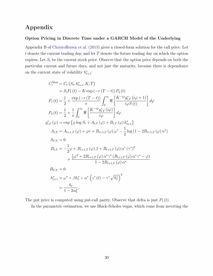
Appendix

Option Pricing in Discrete Time under a GARCH Model of the Underlying

Appendix B of Christoffersen et al. (2013) gives a closed-form solution for the call price. Lett denote the current trading day, and let T denote the future trading day on which the optionexpires. Let St be the current stock price. Observe that the option price depends on both theparticular current and future days, and not just the maturity, because there is dependenceon the current state of volatility h∗t+1:

CModi = Ct

(St, h

∗t+1, K, T

)= StP1 (t)−K exp (−r (T − t))P2 (t)

P1 (t) =1

2+

exp (−r (T − t))π

ˆ ∞0

<[K−iϕg∗t,T (iϕ+ 1)

iϕS (t)

]dϕ

P2 (t) =1

2+

1

π

ˆ ∞0

<[K−iϕg∗t,T (iϕ)

iϕ

]dϕ

g∗i,T (ϕ) = exp{ϕ logSt + At,T (ϕ) +Bt,T (ϕ)h∗t+1

}At,T = At+1,T (ϕ) + ϕr +Bt+1,T (ϕ)ω∗ − 1

2log (1− 2Bt+1,T (ϕ)α∗)

AT,T = 0

Bt,T = −1

2ϕ+Bt+1,T (ϕ) β +Bt+1,T (ϕ)α∗ (γ∗)2

+12ϕ2 + 2Bt+1,T (ϕ)α∗γ∗ (Bt+1,T (ϕ)α∗γ∗ − ϕ)

1− 2Bt+1,T (ϕ)α∗

BT,T = 0

h∗t+1 = ω∗ + βh∗t + α∗(z∗ (t)− γ∗

√h∗t

)2

=ht

1− 2αξ.

The put price is computed using put-call parity. Observe that delta is just P1 (t).In the parametric estimation, we use Black-Scholes vegas, which come from inverting the

30

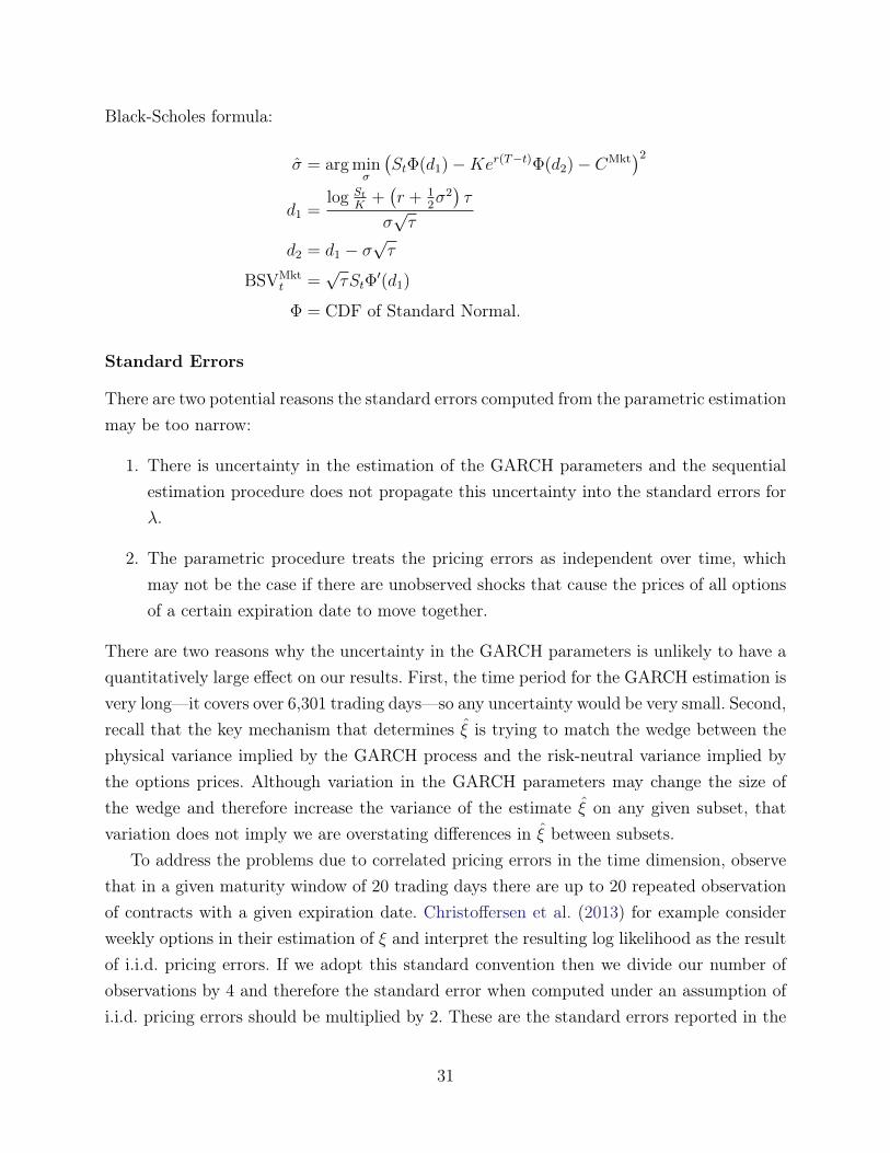
Black-Scholes formula:

σ = arg minσ

(StΦ(d1)−Ker(T−t)Φ(d2)− CMkt

)2

d1 =log St

K+(r + 1

2σ2)τ

σ√τ

d2 = d1 − σ√τ

BSVMktt =

√τStΦ

′(d1)

Φ = CDF of Standard Normal.

Standard Errors

There are two potential reasons the standard errors computed from the parametric estimationmay be too narrow:

1. There is uncertainty in the estimation of the GARCH parameters and the sequentialestimation procedure does not propagate this uncertainty into the standard errors forλ.

2. The parametric procedure treats the pricing errors as independent over time, whichmay not be the case if there are unobserved shocks that cause the prices of all optionsof a certain expiration date to move together.

There are two reasons why the uncertainty in the GARCH parameters is unlikely to have aquantitatively large effect on our results. First, the time period for the GARCH estimation isvery long—it covers over 6,301 trading days—so any uncertainty would be very small. Second,recall that the key mechanism that determines ξ is trying to match the wedge between thephysical variance implied by the GARCH process and the risk-neutral variance implied bythe options prices. Although variation in the GARCH parameters may change the size ofthe wedge and therefore increase the variance of the estimate ξ on any given subset, thatvariation does not imply we are overstating differences in ξ between subsets.

To address the problems due to correlated pricing errors in the time dimension, observethat in a given maturity window of 20 trading days there are up to 20 repeated observationof contracts with a given expiration date. Christoffersen et al. (2013) for example considerweekly options in their estimation of ξ and interpret the resulting log likelihood as the resultof i.i.d. pricing errors. If we adopt this standard convention then we divide our number ofobservations by 4 and therefore the standard error when computed under an assumption ofi.i.d. pricing errors should be multiplied by 2. These are the standard errors reported in the

31

plots and figures for the parametric estimation. Note that no similar correction needs to bemade for the Sharpe ratios as those look at returns, which would still be independent if therewere a persistent shock that raised prices.

32