Swedish Bonds TermStructure Modeling with The

Nelson Siegel Model

Malick Senghore

Bachelors Thesis (2013). Lund University, Sweden.

CONTENTS

ACKNOWLEDGEMENT 1

1 BACKGROUND AND INTRODUCTION 2

1.1 Background 2

1.2 Introduction 3

2 INTEREST RATES THEORY 4

2.1 Discount factor 4

2.2 The Stochastic discount factor 5

2.3 Zero Coupon bonds 6

2.3.1 The Yield Curve 7

2.4 Coupon Bonds 9

2.4.1 Fixed Coupon Bonds 10

2.4.2 The Yield To Maturity 11

2.4.3 Floating rate notes and Variable rate notes 12

2.5 The Day-Count Convention and The Compounding Types 12

2.5.1 Day-Count Convention (year fraction) 13

2.5.2 Compounding Types 13

2.5.3 Continuously compounded interest rates 13

2.5.4 Simply compounded rate 14

2.5.5 Annually-compounded spot interest rate 15

2.5.6 k-times-per-year compounded spot interest rate 15

2.6 Interest rates assets 16

2.6.1 Forward Rate 16

2.6.2 Forward Rate Agreement (FRA) 16

2.6.3 Interest rate Swaps 18

i

ii

2.6.4 Future Contract 20

2.6.5 Caps and Caplets 20

2.6.6 Floor and Floorlets 21

2.7 Swaptions 21

3 LINEAR SYSTEMS 23

3.1 Linear processes 23

3.2 White Noise 23

3.2.1 Moving Averages (MA) 24

3.2.2 Autoregressive processes AR 24

3.2.3 ARMA processes 25

4 DYNAMIC MODELS 26

4.1 Vector Autoregressive Process (VAR) 26

4.2 State Space Modeling 26

4.2.1 The Kalman Filter 27

5 THE NELSON-SIEGEL MODELS 30

5.1 Nelson-Siegel Model Classes 31

5.1.1 Three-factor base model 31

5.1.2 Two-Factor Model 33

5.1.3 Four-Factor Model 33

6 APPLICATION OF THE NELSON SIEGEL MODEL 36

6.1 Intuition Behind The Three Factor Nelson Siegel Model 36

6.2 Data 37

6.3 Descriptive Statistics, data 39

6.4 Estimation of model parameters 40

6.5 Analysis 41

6.5.1 Modeling the Estimated Factors 44

6.6 Conclusion 49

BIBLIOGRAPHY 50

ACKNOWLEDGEMENT

My sincere thanks and gratitude to lecturer and supervisor Magnus Wiktorsson,without whom this thesis would not have materialized. Thank you very much foryour help, support and patient.

1

Chapter 1

BACKGROUND ANDINTRODUCTION

1.1 Background

Fixed income securities, also known as bonds, are one of the most commonly usedloan instruments by governments, private companies and financial intermediaries toraise funds. For instance, they are used by governments to finance budget deficitsand public expenditures, by private companies to finance current and future invest-ments and by banks and other financial intermediaries to finance loans to householdand companies.

The price paid or required by the participants in the credit market, where fixedincome securities are traded, is referred to as interest. In other words, interest isthe compensation required to loan out money, or the cost of taking a loan.

Interest rates affects many aspects of our lives in many different ways. Fromdecisions on mortgages, buying and selling of assets (both real and financial), privateand government investments, monetary policies to stimulate economic growth bothin the short- and long run, etc. It is therefore imperative to understand interestrate and its role in the financial system and the society as a whole. The knowledgeon interest rates will help us to take rational decisions on private economic issues,as well as in understanding and taking part in political debates on macroeconomicissues. Moreover, the very idea that money can be traded at a price is fascinatingin itself.

There exist a variety of fixed income securities in the market for both short-and long maturities as well as fixed or variable interest rates and also a variety ofmodels to model, estimate and forecast their term structures.

2

Section 1.2. Introduction 3

1.2 Introduction

Swedish government bonds will be the main focus of this thesis. The money marketin Sweden, (i.e the market in which Swedish government bonds with maturitiesless a year are traded), develops from a regulated system in the seventies to a welldeveloped and functioning international market as we know it today.

Under the early eighties, the fixed security market starts to take shape in Swe-den, with the introduction of certificates of deposits issued by banks. The bankswere able to loan money, from the general public, for a fixed interest and withminimal risk. In 1982, the first zero-coupon bonds were issued by the Swedish gov-ernment, thus enabling them to loan money directly from companies and privateinvestors instead of the banks. In 1983, the concept of zero-coupon bonds was thenextended to other sectors of the society, municipalities started issuing municipalbonds, companies started issuing commercial papers, financial companies startedissuing market evidence in other to finance their lending to households and compa-nies, Swedish Housing Finance Institutions started issuing mortgage bonds. The firstSwedish government coupon bonds, called National Bond 1001 with maturity date1987, were also issued by the Swedish government through the Swedish NationalDept Office in 1983.

The development of the money market in Sweden can be attributed to threemain factors, namely, the emergence of a securities market, deregulation of thefinancial system and the arrival of a derivatives market in Sweden. Most of thedevelopment occurs in the early eighties.

In this thesis, we fit Swedish government bonds with a well known parametricterm structure model namely, the Nelson Siegel model. The Nelson-Siegel Modelclasses are very popular and widely used by practitioners and Central Banks. Theirpopularity is buried in the model’s simplicity and ability to fit the various shapes andforms the term structures of interest rates can exhibit and providing economicallyand statistically meaningful and correct results.

The Diebold and Li (2006) two-step approach of the three-factor Nelson Siegelmodel will be applied to Swedish government bonds and we will show that thisapproach models well the yields on Swedish government bonds.

We now proceed by going through the theory on interest rates, followed by abrief description of linear and dynamic stationary processes. In the dynamic system,state space representation will be introduce and the state equation used to representthe dynamics of the model co-efficients. The Nelson-Siegel model classes will beintroduced and presented as factor models. Finally, the three-factor Nelson-Siegelmodel will be applied to Swedish government bonds. Using ordinary least squares,factor dynamics are obtained for each cross-section of the data. A time series model,namely independent stable AR(1) processes, is then fitted to the factors. The resultsobtained will be contrasted with the data and an in-sample-fit reported.

Chapter 2

INTEREST RATES THEORY

In every well developed market economy, there is the need for households, firms andgovernments to finance loans, investments and budget deficits by borrowing moneyat a price. There is also the need to save excess income for future consumption,profits for future investments and budget surpluses for future government expendi-tures. The price demanded to lend out money or the cost incurred for taking a loanis referred to as Interest rate.

The need to borrow and lend money is satisfied in the credit market, where theactors acquire financial assets such as bank accounts, stocks, bonds, etc throughfinancial intermediaries, by entering in a contact or an agreement. These financialassets gives the holder the right/option and the issuer the obligation to fulfill thecontract/agreement at a pre-specified date stipulated in the contract.

We will start our journey to understanding interest rates by going through somebasic interest rate theory.

We are all familiar with the saying that a dollar today is worth more that adollar tomorrow. This is normally shown to be true by using a simple but powerfulformula called the present value formula. This leads us to the discounting factorthat depends on the simple- or effective interest rate, the day-count convention andthe time to maturity of the future cash flow.

2.1 Discount factor

To enable us to make a decision on whether to invest on a financial/real asset ornot, we need to know how much consumption we are forgoing today in other toincrease our consumption in the future. This is can be computed by discounting allthe future cash flows of our investments with a discounting factor.

The discount factor helps to relate the present value of a future cash flow. It isa function of the future cash expected, time to maturity and the interest rate onthe instrument in question. The bank account, also known as the money marketaccount will be used to describe the discount factor.

The bank account describes how an amount of money deposited in a bank, witha fixed positive instantaneous rate r, grows over time. If we let Bt denote the valueof a bank account at time (t ≥ 0), then the bank account grows according to the

4

Section 2.2. The Stochastic discount factor 5

differential equation:

dBt = rBtdt (2.1.1)

B0 = 1 (2.1.2)

where r is a positive function of time.This implies that, the amount of money in the bank account at time t will grow to:

Bt = exp

(∫ t

0

rds

)(2.1.3)

The instantaneous interest rate rt used in the discounting factor to obtain thepresent value of the money market account is composed of, amongst other things,the compensation for the lender for forgoing consumption today for future date,the compensation for increases in future price levels (i.e. inflation) as well as arisk premium for the lenders exposure to default risk. All these three componentstogether is what is collectively referred to the interest rate on a loan or an I.O.Uinstrument.

Note: A promise to pay a debt, especially a signed paper stating the specificamount owed and often bearing the letters I.O.U

2.2 The Stochastic discount factor

Our goal in interest rate theory is to study and understand the variability of interestrates. We therefore allow the interest rates to be stochastic, as indeed, they are theunderlying assets of interest.

When the spot rate in the discount factor is allowed to be stochastic, we thusobtain a stochastic discount factor.

The Stochastic discount factor D(t,T), is basically used to relate amounts ofmoney at two different time points t and T. It is the amount at time t that isequivalent to one unit of currency (the nominal amount) payable at time T, and isgiven by:

D(t, T ) =BtBT

= exp

(∫ T

t

rsds

)The stochastic discount factor leads us to the simplest form of loans in the money

market, namely the Zero-Coupon Bonds. Zero-coupon bonds provides their holderwith a deterministic amount, that is known when the bond is issued. Zero-couponbonds are also referred to as discount bonds as they are traded at a discount totheir face value. They are one of the main building blocks of interest rate theory.

6 Interest rates theory Chapter 2

2.3 Zero Coupon bonds

Zero-coupon bonds are the simplest form of loan in the credit market. They haveonly one payment stream under their whole lifetime, that is, the face value of thebond payable to the bond holder at maturity. However, zero-coupon bonds arein practice not directly observable in the market and long maturities zero-couponbonds are not traded at all, due to for example credit-risk.

The price of a zero-coupon bond is obtained by discounting its nominal valueswith a stochastic discounting factor. The price is therefore a function of the zero-coupon interest rate, time to maturity and the face value of the bond.

The short rates are the rates that prevails in the money market and can directlybe control by Central Banks policies. This can be done through monetary poli-cies, given a variable foreign exchange rate policy, by open market interventions orthrough repurchase agreement rates. For example, in Sweden, increasing/decreasingthe money supply lowers/increases the short rate.

The long rates are governed by the expected short-rates, inflation and the riskpremium on the bond. The risk premium, which can be either positive or negative,is the expected returns on a bond with a fixed rate, in relation to a series of short-term investments.

Formally, a zero coupon bond that matures at time T (also called a T-bond) isdefined as follows:

Definition 2.1. A T-maturity zero-coupon bond is a contract that guarantees itsholder the payment of one unit of currency (the nominal amount) at time T, withno intermediate payments. The contract value, i.e the price of a zero coupon bondat time t < T is denoted by P(t,T) and P(T,T) = 1 for all maturity times T isequal to the present value of the nominal amount which can be written as:

P (t, T ) =P (T, T )(

1 + r × d360

)T−t (2.3.1)

where r is a deterministic interest rate and d refers to number of days remainingfor the bond to mature. Note that r is also the internal rate of return on the bond,i.e. the bond yield.

The discount factor and the zero-coupon bond price are very much related, inthe sense that they both give the present value of a future cash flow, but with asignificant difference been, the price of a zero-coupon bond is a value of a contractand the discount factor is an amount of money.

Normally zero-coupon bonds are treated as risk free assets, due to the determin-istic cash flow they provide its holder. They are therefore widely used in portfoliodiversification and hedging. However, the cash flow from bonds in general is onlydeterministic if it is exercise at maturity, otherwise there are basically three typesof risk associated with bonds namely, interest rates risk, credit risk and inflationrisk.

Section 2.3. Zero Coupon bonds 7

As mentioned earlier, the price of a zero-coupon bond is a stochastic processwith two random variables, t and T. If T is fixed, then the contract price, denotedby P(t,T), will be a scalar stochastic process. It gives the prices at different timesfor a bond with fixed maturity T and its trajectory is very irregular.On the other hand, if t is fixed, then the contract price is a smooth function ofmaturities, for T > t. Given a fixed t, a fundamental curve which can be obtainedfrom observed interest rates is referred to as the zero-coupon curve or the yieldcurve.

2.3.1 The Yield Curve

The yield curve describes the relationship between the returns on bonds (i.e theyield) with the same credit-risk but with different maturities. It is widely used tocompare yields offered for different maturities. The yield curve is also known as theterm structure of the discount factors. Formally we can define the yield curve attime t as:

Definition 2.2. The yield curve at time t, is the graph of the function:

T 7→ P (t, T ), T > t (2.3.2)

which decreases with maturity T .

In the Swedish bond market, bonds with maturities less than a year are quotedas simple interest rates and those with maturities more than a year are reportedas effective rates. In constructing a yield curve for the whole tenor structure, wetherefore need to convert the simple rates into effective rates in other to make surethat we are comparing rates with the same credit-risk. Theoretically, only effectiverates for zero-coupon bonds guaranteed risk-free return if hold until maturity.

Note, the term yield curve is often used to denote several different curves de-duced from quotes from the interest-rate-market. That is to say, there exist otherrepresentations of the yield curve different from the one defined in definition 2.2.Thus, a yield curve that is a function both the short and long rate can be describedas follows:

Definition 2.3. The yield curve at time t is the graph of simply compounded interestrates for maturities T less than one year and the annually compounded interest ratesfor maturities more than a year.

T 7→

L(t, T ) t < T ≤ t+ 1 (years),

A(t, T ) T > t+ 1 (years).(2.3.3)

where L(t,T) and A(t,T) are as described in 2.5.4 and 2.5.8 respectively.

The slope of the yield-curve varies over time and assumes different shapes andforms, which is a reflexion of the values of the short and the long yields. The

8 Interest rates theory Chapter 2

yield-curve slope is sometimes used as a future gross domestic product and inflationdevelopment indicator. Depending on its slope, the yield-curve can be classify intothree main categories namely, normal-, inverted- or flat yield.

Normal Yield Curve: A yield curve is called normal if it has a positive slope withshort-rates being lower than long-rates. This can occur when an economy ismoving from a period of recession into a period of growth. A normal yieldcurve can be indicating higher inflation rates are expected which increases thelong-rates.

Inverted Yield Curve: The inverted yield curve have a negative slope and itoccurs if short-term yields are higher than long-term yield. An inverted yieldcurve is usually observed when an economy is at the top of its business cycleor under great stress. This signals the coming of a weak business cycle andhence lower inflation rates thereby causing the long rates to fall.

Flat Yield Curve: If the yield curve have a zero slope, then we have a flat yieldcurve. This occurs if there exist little or no significant difference betweenshort-term yields and long-term yield.

In trying to understand the different slopes, shapes and forms assumed by theyield-curve, economics have come up with different explanations and hypothesis,amongst them include, the expectation hypothesis and the preferred habitat hypoth-esis.

The Expectation Hypothesis: This is the most well known hypothesis used intrying to explain the theory behind the shape of the yield curve. It is basedon three main assumptions:

1. All investors are risk neutral, in the sense that they lack preferences forbonds with certain maturities and therefore do not demand risk com-pensations on their investments. It is also assumed that investors in thebond markets have rational expectations.

2. The yield curve conveys all the information in the market, i.e. the ex-pectation hypothesis assumes that the bond market is effective.

3. If there exist arbitrage between bonds with different maturities, investorscan establish a yield curve that is consistent with how rates are expectedto developed over time.

The assumptions made in the expectation hypothesis implies that future in-terest rates can be read from the yield curve, and the expected returns are thesame and independent of the investment strategy we choose. For example, aone month investment in a three-year bonds gives the same return as a onemonth investment on a five-year bond.

Section 2.4. Coupon Bonds 9

The Preferred Habitat Hypothesis: This can be seen as an extension of theexpectation hypothesis, were investors prefers certain maturities to othersand therefore demands compensation, in the form of a risk premium, forinvestments in bonds with maturities that deviates from their preferences.This hypothesis can be categorized into two, depending on the preference ofthe investor.

1. Liquidity preference theorem implies that investors, prefer bondswith short maturities to bonds with longer maturities (i.e. consumptiontoday is preferred to consumption tomorrow). The risk averse investorstherefore demands a risk premium for investing in bonds with long matu-rities and the longer the maturity, the more risk premium is demanded.Here, the yield-curve tends to have a more positive slope than that ofthe expectation hypothesis.

2. The market segmentation theorem assumes that bond investors andissuer by law, preference or habit invests and issue bonds with certaintype of maturities. For example, banks normally prefer short maturitybonds whereas insurance companies and pension funds prefer long ma-turity bonds.Note that the yield-curve under the market segmentation theorem cannotbe used to analyze market expectations of future interest rates, since itis not directly based on the outcome market forces, supply and demand.

It is important to note that Central Banks can also affect the shape of the yieldcurve through the confidence and trustworthiness the market has on their ability tostabilize inflation. For example, if the actors in the market believes that the CentralBank can stabilize the inflation rates to an acceptable level, then the yield curvereflexes the expected future long rates which in turn becomes less volatile compareto the short rates.On the other hand, if the market does not believe in the ability of the CentralBank to control the inflation rate, then both the long and short rates will be highlyvolatile.

It is appropriate to now mention another type of bond that is very much similarto a zero-coupon bond, and well traded in the markets, called the coupon bonds.The main difference between a coupon bond and a zero-coupon bond is that theformer pays coupons to the bearer at periods stipulated in the contract, which caneither be annually (as in Sweden) or every six months (as in the USA).

2.4 Coupon Bonds

Zero-coupon bond are not very well traded in the markets and those markets thatdo trade in them, trade in zero-coupon bonds with very short maturity (i.e. lessthan a year). What is traded in the market arecoupon bonds with maturities morethan a year. In addition to the face value of the bond, the bearer of a coupon bond

10 Interest rates theory Chapter 2

receives periodic coupon payments called the the coupon rates.It is worth mentioning that the coupon rate is different from the market rate.

The market rate is the rate at which bonds are traded at the present moment, in thebond market. The market rates varies overtime and can therefore directly affectsthe bond price and hence it market value. The coupon rates on the other hand, area fixed percentage of the nominal amount and is stipulated in the contract.

Coupon bonds can be classified into two main categories, depending on whetherthey pay a fixed coupon rate or a variable coupon rate. The two categories aredescribe below:

2.4.1 Fixed Coupon Bonds

This is the simplest coupon bond. It is a bond, which for some intermediate pointsin time, will provide the holder with predetermined payments.Formally, a fixed coupon bond that matures at time T can be described as follows:

Definition 2.4. Given a tenor structure, T0, T1, . . . , Tn, a coupon bond is a contractentered at time T0 that guarantees its holder the payment of the nominal amount ofthe bond at time Tn, with intermediate determined payments (called coupons) Ct attimes T1, . . . , Tn.The contract value, i.e the price of a coupon bond at time T0 is denoted by P(t,T)and P(T,T) = 1 for all maturity times T, is equal to the sum of the discountedfuture cash flows which can be express as:

p(t) =

n∑t=1

Ct(1 + ri)t

+P (T, T )

(1 + rn)n(2.4.1)

where rt for t = 1, 2, . . . , n , is the effective interest rate.

The fixed coupon bonds can be replicated by holding a portfolio of zero couponbonds with maturities Ti, for i = 1, 2, . . . , n. That is, we pay Ci zero coupon bondsof maturities Ti for i = 1, 2, . . . , n − 1 and A + Cn bonds with maturity Tn. Withthis portfolio, for a time t < T1, we can price the coupon bonds as:

p(t) = A× P (t, Tn) +

n∑i=1

Ci × P (t, Ti) (2.4.2)

The coupon bonds are quoted mostly in term of returns on the face value A overa given period [Ti−1, Ti] and not in monetary terms. For example, given that theith coupon has a return equal to ri, this implies

ci = ri × (Ti − Ti−1)×A (2.4.3)

If the interval lengths are equal (i.e. Ti = T0 + iδ) and the coupon rates for eachinterval is equal to a common rate r, then we have a standardize coupon bond.

Section 2.4. Coupon Bonds 11

The price p(t), for t < T1, of a standardized coupon bond is given by:

p(t) = A×(P (t, Tn) + rδ

n∑i=1

P (t, Ti)

)(2.4.4)

As observed from the pricing formula of the coupon bond above, different pay-ments are discounted with different effective rates. This makes it difficult to relatethe price of the bond to a single effective rates. This problem can be overcome byquoting the bond with a single interest rate that is derived from the bond marketprice. This single rate, with which all future cash flows of the bond, both couponsand face value, is discounted and re-invested is referred to as the yield to maturity.

2.4.2 The Yield To Maturity

The yield to maturity gives the bonds internal rate of return, i.e. the return oninvestments that describes the present values of all future cash flows. Thus, theyield to maturity is the single effective interest rate that makes the price of thebond today to be equal to its market price.

Given the price P(t,T), of a bond and its coupon payments Ct, the yield tomaturity can be obtained from the pricing formula of a coupon bond by solving fory in the formula below:

P (t, T ) =

n∑t=1

Ct(1 + y)i

+P (T, T )

(1 + y)n(2.4.5)

One should be very careful in how the yield to maturity is interpreted. This isbecause the yield to maturity implicitly assumes that the yield curve is completelyflat, i.e. the interest rates are the same for the whole investment period which is notthe case. Future interest rates are generally unknown and varies depending mainlyon what stage in the business cycle an economy is in.

The yield to maturity does not provide a deterministic return since there is al-ways a re-investment risk for each and every coupon payment.The yield to maturity tells us nothing about the interest rates on other bonds, asit only consider the bond for which its internal rate of return is been computed.There is also the risk that different yield to maturity for different bonds can be in-terpreted as a possibility to reinvest coupons at different rates, whereas the couponsare re-invested at the market rates.

There is a yield to maturity that is of particular interest to investor, i.e. thepar yield. The par yield is the coupon rate which makes the bond price equal toits nominal value.

There exist a variety of coupon bonds in the market, with some bonds havingphysical assets as their underlying. These types of bonds are called mortgagebacked/asset backed securities. The advantages of investing in these types ofbonds is vested on the credit worthiness of the issuer and the market value of theunderlying. There also exist bonds whose value is tied to a certain price index.

12 Interest rates theory Chapter 2

These bonds guard the holders against inflation and are called inflation-linkedbonds.However, we are only interest in loan instruments issued by governments and willtherefore not consider the above mentioned bonds. Government bonds do offercoupons with rates that varies depending on a benchmark rate. Bonds with varyingrates are generally referred to as floating rate notes.

2.4.3 Floating rate notes and Variable rate notes

There are numerous coupon bonds for which the value of the coupon is not fixed atthe time the bond is issued, but rather reset for every coupon period. Mostly, butnot always, the resetting is determined by some financial benchmark, for example,in Sweden, the three months STIBOR rates is normally used. One of the simplestfloating rate bonds quotes the STIBOR rate plus/minus a certain amount of basispoints. The amount of basis points demanded by investors is solely determined bythe credit worthiness of the bond issuer.

The floating rate bonds can be replicated by using a self-financial bond strategy,with an initial cost P (t, Ti−1) at time t and reinvesting the amount receive at timeTi−1 in bonds that matures at time Ti. Thus the price p(t) for the floating ratebonds, given that the coupon dates are equally spaced (i.e. Ti = T0 + iδ) andassuming that the face value equals to one, for time t < T1 is given by:

p(t) = P (t, Tn) +

n∑i=1

[P (t, Ti−1)− P (t, Ti)] = P (t, T0). (2.4.6)

In particular, if t = T0, then p(T0) = 1.

It is important to note that some assumptions must be made to guarantee theexistence of a market that is sufficiently rich and regular where these bonds aretraded. That is, we have to assumed that there exists a frictionless market for zero-coupon bonds for every maturity time T and that the price of a zero-coupon bondP (t, t) = 1 for all times t. The assumption that P (t, t) = 1 is necessary to ensurethat we avoid arbitrage pricing. We also have to assumed that for each fixed timet < T , the price of a zero-coupon bond that matures at time T is differentiable withrespect to the time of maturity T .

Now we discuss two fundamental features of the interest rates. These features arethe Day-Count convention and the Compounding-Type. The role of these featureswere briefly observed in the present value formula. Below, we discuss them in moredetail.

2.5 The Day-Count Convention and The Compounding Types

The compounding types and the day-count convention are the two fundamentalproperties of interest rates that are needed to enable us to used zero-coupon bondsto price interest rates.

Section 2.5. The Day-Count Convention and The Compounding Types 13

2.5.1 Day-Count Convention (year fraction)

The day-count convention is a fraction of a year that helps us to compute theinterest payable and the end of an interest- or loan period. It tells us how intereston an investment grows over time. The numerator represents the number of daysin the interest- or loan period and the denominator represents the number of daysin the reference period. We denote by τ(t, T ), the chosen time measure between tand T, which is usually referred to as year fraction between the issuing date t andmaturity date T. When t and T are less than one-day distant, then τ(t, T ) is to beinterpreted as the time difference, i.e. (T-t) in years. It is important to mentionthat there are various type of day count conventions used, depending on the markettype, country and currency been used. However, for our purpose, we will used theSwedish convention, where the reference period is 360 days.

2.5.2 Compounding Types

The compounding type refers to how the interest rate is computed based on boththe initial principal amount invested and the interest generated in earlier peri-ods. Basically, the compounding types can be classified into four main categories,namely continuously-compounded rates, simply-compounded rates, k-times-per-yearcompounded rates and annually-compounded rates. Of these four compoundingtypes, the simply-compounding type, also called the LIBOR rates, is the mostcommonly used both in theory and in practice. The compounding types can beexpress as forward rates or spot rates. Below, a description of the above mentionedcompounding types are given.

2.5.3 Continuously compounded interest rates

Basically, continuously compounding rate is the constant rate prevailing on an in-vestment on a zero-coupon bond at time t, for maturity at a future time interval[S, T ], that yields a unit of currency at time of maturity.

If the contracting date coincides with the start of the interval, then we have acontinuously-compounded spot rate, otherwise a continuously-compounded forwardrate. The continuously compounded spot and forward rates are describe below:

The continuously compounded forward rate contracted at time t for the pe-riod [S, T ] is defined as

R(t;S, T ) = − logP (t, T )− logP (t, S)

τ(T, S)(2.5.1)

The continuously compounded spot rate contracted at time S for the period[S, T ] is defined as:

R(S;S, T ) = − logP (S, T )

τ(T, S)(2.5.2)

14 Interest rates theory Chapter 2

The continuously compounded spot rate is a constant rate, from which we canderive the price of a zero coupon bond as

R(S;S, T )× τ(S, T ) = − logP (S, T ) (2.5.3)

⇒ P (S, T ) = exp(R(S, T )× τ(S, T )) (2.5.4)

2.5.4 Simply compounded rate

When accruing occurs proportionally to the time of the investment then we have asimply compounded spot rate. The simply compounded rate is also referred to asthe LIBOR rates, L(t, T ). This is the rate used most commonly in the market.

The LIBOR Interest Rates

LIBOR stands for London Interbank Offer Rate. It is the average rate with whichBanks on the London money market are prepared to borrow and lend money toeach other. The LIBOR rates are quoted in ten different currencies and comesin fifteen different maturities. Changes in the LIBOR rates are closely monitoredby all actors in the financial market, because it is generally used as the base rateby banks and other financial institutions. Thus a change in the LIBOR rates willimpact saving accounts, mortgages, loans, etc.

The LIBOR rate prevailing at time t for the maturity T, is the constant rate atwhich an investment has to be made to produce one unit of currency at maturity,starting from P(t,T) units of currency at time t, when accruing occurs proportionalto the investment time.

LIBOR are forward rates that can either be quoted as continuously compoundedrates or simple rates. The simple rates notation is the one most commonly used inthe markets, whereas the continuously compounded notation is used for theoreticalpurposes. The simple LIBOR rate can be quoted as forward rates or spot rates asfollows:

The simple forward rate contracted at time t for the period [S, T ] is called theLIBOR forward rate and is defined as

L(t;S, T ) = −P (t, T )− P (t, S)

τ(T, S)P (t, T )(2.5.5)

The simple spot rate contracted at time S for the period [S, T ] is called theLIBOR spot rate and it is defined as:

L(S;S, T ) = −P (S, T )− P (S, S)

τ(T, S)P (S, T )(2.5.6)

Section 2.5. The Day-Count Convention and The Compounding Types 15

2.5.5 Annually-compounded spot interest rate

The annually compounded spot rate prevailing at time t for maturity T is denotedby A(t, T ), and is the constant rate at which an investment has to be made toproduce an amount of one unit of currency at maturity, starting from P(t,T) unitsof currency at time t, when reinvesting the obtained amount once a year.

A(t, T ) =1

[P (t, T )]1

τ(t,T )

− 1 (2.5.7)

⇒ P (t, T ) =1

[1 +A(t, T )]τ(t,T )(2.5.8)

2.5.6 k-times-per-year compounded spot interest rate

The k-times-per-year compounded spot interest rate prevailing at time t for thematurity T is denoted by Ak(t, T ) and is the constant rate at which an investmenthas to be made to produce an amount of one unit of currency at maturity, startingfrom P(t,T) unit of currency at time t, when reinvesting the obtained amount ktimes a year.

Ak(t, T ) =k

[P (t, T )]1

kτ(t,T )

− k (2.5.9)

⇒ P (t, T ) =1[

1 + Ak(t,T )k

]kτ(t,T )(2.5.10)

Observe that the continuously compounded spot interest rate can be obtained as thelimit of the k-times-per-year compounded rates, where the number of compoundingtimes k going to infinity. Indeed

limk→+∞

k

[P (t, T )]1

kτ(t,T )

− k = R(t, T )

All the spot rates mentioned above are equivalent in infinitesimal time intervals.Indeed

r(t) = limT→t+

R(t, T ) (2.5.11)

= limT→t+

L(t, T ) (2.5.12)

= limT→t+

A(t, T ) (2.5.13)

= limT→t+

Ak(t, T ) for each k (2.5.14)

16 Interest rates theory Chapter 2

2.6 Interest rates assets

Derivatives that have interest rates as underlying assets, (i.e. interest rate for-wards/futures, caps/caplets, floors/floorlets, swaps, swap contracts, etc), are usedby many actors in the financial market for varying purposes. For example, specu-lators in the interest rate market uses interest rate derivatives to beat the marketsreturns . Arbitragers used a combination of interest rate derivatives in other tomake a risk-free profit and hedgers used them in their portfolios in other to reducedrisk.

We will now introduce forward- and future contract that were first used tohelp farmers hedge their agricultural produces against price-risk . In our case, wewill study these contracts with interest rates, rather than agricultural produces, asunderlying assets.

2.6.1 Forward Rate

The basic construction for interest rates assets is the forward rate and it is usedto adjust for interest rate risk. Forward rates are interest rates that can be lockedin today for an investment in a future time period, and are set consistently withthe current yield of discount factors. Generally speaking, the holder of a forwardcontract has the obligation to buy or sell a certain product at a future date fora given price. It is a bilateral agreement between two actors, (for example, twobanks or a bank and a company). The forward contract can be constructed in anyway that suits the two parties involved. Forwards are traded Over The Counter(O.T.C), i.e. no exchange market is involved. The forward contract has only onecash flow that is paid at the maturity date.The forward rate is characterized by three time instances, namely the contract datet, the date the contract is effective S and the exercise date T, where t < S < T .

A forward rate can be defined as:

Definition 2.5. Given three fixed time points t < S < T , a contract at time t whichallows an investment of a unit amount of currency at time S, and gives a risk lessdeterministic rate of interest over the future interval [S, T ] is called The forwardrate.

Note that spot interest rates are forward rates where the time of contractingcoincides with the start of the interval over which the interest rate is effective (i.e.t = S).

Another way to define the forward rates is through a Forward Rate Agreement.By demanding that the forward rate agreement be fair, we have the forward rate.

2.6.2 Forward Rate Agreement (FRA)

Basically the FRA allows one to lock-in the unknown interest rate in a future timeinterval with a desired value that is agreed upon today. A forward rate agreementis therefore a contract that involves three time instances:

Section 2.6. Interest rates assets 17

1. t: the time at which the rate is considered

2. S: maturity time

3. T: expire time

such that t < S < T . The contract gives its holder an interest-rate payment for theperiod between T and S. At the maturity time S, a fixed payment based on a fixedrate K is exchanged against a floating payment based on the spot rate LIBOR thatresets in S with maturity T, i.e. L[S,T].At time T one receives (τ(S, T ) ×K × A) units of currency and pays the amount(τ(S, T ) × L(S, T ) × A), where A is the contract nominal value. The value ofthe contract, which can be both positive (when K > L(S, T )) or negative (whenK > L(S, T )), is given by :

A× τ(S, T )× [K − L(S, T )] (2.6.1)

Thus the total value of the forward rate agreement at time t is given by:

FRA(t, S, T, τ(S, T ), A,K) = A× [P (S, T )× τ(S, T )×K - P (t, S) - P (t, T )]

The forward rates can be classified into two main groups namely, simply-compoundedforward interest rate and Spot forward interest rate.

Simply-compounded forward interest rate

The rate K, that renders the FRA arbitrage free at the contract date is obtained byequating the value of the forward rate agreement to zero. This value thus obtainedis called the simply-compounded forward interest rate. It is the value of the fixedrate in a prototypical FRA with expiry S and maturity T that renders the FRA afair contract at time t.The simply-compounded forward rate can be viewed as an estimate of the futurespot rate LIBOR/STIBOR. It is a random quantity, based on market condition atthat time. It can be shown that, under a suitable probability measure, the simplycompounded forward interest rate at time t is the expectation of the of the spotLIBOR at time t.

The simply compounded forward interest rate prevailing at time t for expiryS > t and maturity T > S is denoted by F (t;S, T ) and is defined by :

F (t;S, T ) :=1

τ(S, T )

(P (t, S)

P (t, T )− 1)

Using the simply compounded forward interest rate, the forward rate agreementcan be written as:

FRA(t, S, T, τ(S, T ), A,K) = A× P (t, T )× τ(S, T )× [K − F (t;S, T )]

18 Interest rates theory Chapter 2

Therefore to value the FRA, we just need to replace the LIBOR rate L(S,T) inthe payoff function with the corresponding forward rate F(t;S,T) and then take thepresent value of the resulting deterministic quantity. When the maturity of theforward rate collapses towards its expiry, we have the instantaneous forward rate.

Instantaneous forward interest rate

The instantaneous forward interest rates are fundamental quantities in the theoryof interest rates. It is mostly used to express absences of arbitrage opportunity of aninterest rate model by relating certain quantities in the expression of the evolutionof the instantaneous forward interest rate.The instantaneous forward interest rate prevailing at time t for the maturity T > tis denoted by f(t, T ) and is defined as

f(t, T ) := limT→S+

F (t;S, T ) = −∂ logP (t, T )

∂T

so that we also have

P (t, T ) = exp(−∫ T

t

f(t, u)du)

f(t,T) can be seen as forward rates at time t with maturity T very close to expiryS.

A generalization of the FRA is the Interest rate swaps.

2.6.3 Interest rate Swaps

A swap contract, in principle, is an agreement between two parties to exchange aseries of cash flows. An interest rate swap, for a given time interval, is therefore acontract in which the parties exchange a series of interest rate flows with each other.In most cases, one party exchange a variable rate with a fixed rate. Observed that,under the swap agreement, no principle amount is paid out even though the swaprate is computed based this amount.

The swap is considered to be the simplest interest rate contract. A swap contractin which one is able to exchange a payment stream at a fixed rate, the swap rate,for a payment steam at a floating rate (typically the three months LIBOR/STIBORrate) over the future time intervals [T0, T1], [T1, T2], . . . , [Tn − 1, Tn] is called plainvanilla swap or the coupon swap.The swap rate is chosen such that the value of the swap equals zero at the timewhen the contract is made and its given by:

swap rate =1− P (T0, Tn)

δ ×∑ni=1 P (T0, Ti)

(2.6.2)

For face value equal one, the price of the swap contract Πswap(t), for t < T0, ofa swap derivative can be written in terms of the sum of prices of FRA weighted bythe interval lengths [Ti, Ti−1], for i = 1, 2, . . . , n. This sum can be separated into

Section 2.6. Interest rates assets 19

two parts, one that identifies the floating leg and one that identifies the fixed legas.

Πswapt (t) =

n∑i=1

ΠFRAt (Ti−1, Ti) (2.6.3)

=

n∑i=1

(P (t, Ti−1)− P (t, Ti)

)−K ×

n∑i=1

(Ti − Ti−1)× P (t, Ti) (2.6.4)

The first sum in the second equality is the floating leg and its a telescopic sum, thusonly the first and last terms will remain. This gives the swap price, Πswap

t as:

Πswapt (t, Ti, Ti−1) =

n∑i=1

(Ti− Ti−1)×P (t, Ti)×

(P (t, T0)− P (t, Tn)∑n

i=i(Ti − Ti−1)× P (t, Ti)−K

)(2.6.5)

Note that∑ni=1(Ti−Ti−1)×P (t, Ti) is known as the present value of basic points

(PVBP). The swap rate which makes this contract free to enter at time t < T0 is

P (t, T0)− P (t, Tn)∑ni=(Ti − Ti−1)× P (t, Ti)

This leads to two main interest rate assets, i.e. a prototypical payer interest rateswap PFS and a prototypical receiver interest rate swap RFS.

Prototypical payer and receiver interest rate swap

This is a contract that exchanges payments between two different index legs, startingfrom a future time. At every time, Ti in a respecified sets of dates Tα+1, . . . , Tβ thefixed leg, also known as the coupon bearing bond, pays out the amount

A× τi ×K

corresponding to a fixed interest rate K, a nominal value A and a year fraction τibetween Ti−1 and Ti, whereas the floating leg, also known as the floating rate note,pays the amount

A× τi × L(Ti−1 − Ti)

corresponding to the LIBOR/STIBOR rates L(Ti−1−Ti), resetting at the previousinstant Ti−1. Clearly, the floating leg rate resets at dates Tα, Tα+1 . . . , Tβ−1 andpays at dates Tα+1, Tα+1 . . . , Tβ

When the fixed leg is paid and the floating leg is received, we have a payerinterest rate swap, whereas when the fixed leg is received and the floating legpaid we have a receiver interest rate swap.

Requiring that the interest rate swap be arbitrage free at time t leads us to theforward swap rate that is defined as follows:

20 Interest rates theory Chapter 2

The Forward Swap Rate Sα,β at time t, for the sets of times Tα+1, Tα+1 . . . , Tβand year fractions τ , is the rate in the fixed leg of the interest rate swap thatmakes the interest rate swap a fair contract at the present time. This impliesthat

Sα,β =P (t, Tα)− P (t, Tβ)∑β

i=α+1 τiP (t, Ti)

2.6.4 Future Contract

A futures contract supports the main characteristics of a forward contract, withsome significant differences. Futures are standardized contracts, that are traded inwell organized markets, in respect to a delivery date and a given amount. The priceon a futures contract is usually smaller than that of a forward, since the credit-riskof future contracts are much lower than that of a forward contracts. In a futurescontract, there is no delivery of products, instead a cash settlement of profits/losestakes place. There is also a daily contract settlement in the futures market in orderto compensate for price changes. For example, if the price of a future contractincreases from one day to another, then the issuer of the contract is oblige to com-pensate the holder for the price differences.

The most commonly traded derivative products in the interest rate market arecaps/floors and swaptions. The underling assets for the caps/floor are the forwardLIBOR rates and the underlying for the swaptions are swap rates. As mentionedearlier, there are four significant dates in a FRA, namely, the start and the end dateof the accrual period, the payoff date and the fixing date. The complexity of pricingderivative products increases depending on how these date are set. It is thereforeimportant to know the length of time to maturity of the underlying interest rateswap, to determine the set of reset and payment dates. The set of all maturity datesin the contract is often referred to as a tenor structure.

Definition 2.6. A tenor structure, also known as an accrual factor, is a set ofmaturities T = [T0, T1, . . . , Tn], where the first element of the set T0 is typicallystart date and the last elementTn is the end date of the contract. The differencebetween two elements in the tenor structure is called the tenor and is denoted by:

τi = Ti − Ti−1 for i ∈ [1, . . . , N ] (2.6.6)

2.6.5 Caps and Caplets

The cap is one of the most traded of all interest rates derivatives. Generally speak-ing, an interest rate cap is an agreement between two parties (normally a bank and acompany), that if the interest rate on the LIBOR/STIBOR with a certain maturityfor a given period in the future, exceeds a certain level, then the issuer of the capshould compensate the buyer. Interest rate caps are financial insurance contracts

Section 2.7. Swaptions 21

which protects the holder from having to pay more than a pre-specified rate, thecap rate, even though a floating rate loan or I.O.U was taken. The cap rate isdetermined from the difference between interest rate stipulated in the contract andactual interest. Cap contract stipulates, the level of interest rate from which theholder wants protection from, the principle amount and the duration. The cap isdefined as follows:

Definition 2.7. For a given tenor structure Tα, Tα+1, . . . , Tβ, the holder of a caphas the option to receive the forward LIBOR/STIBOR rate τi × L[Ti−1;Ti−1, Ti]and pays a predefined rate τi ×K at the date Ti for (i = α+ 1, . . . , β).In other words the cap is a sum of caplets with payoff function

Πcaplets(L[Ti−1;Ti−1, Ti]) = τi(L[Ti−1;Ti−1, Ti]−K)+

where the payoff date is Ti−1.

Note that the caps relate to the LIBOR/STIBOR as a European call optionrelates to the stock if the forward LIBOR/STIBOR rates increases significantly.

2.6.6 Floor and Floorlets

Interest rate floors are financial insurance contract which guarantee that the interestpaid on a floating rate loan will never be below some predetermined level called thefloor rate.

Definition 2.8. For a tenor structure (Tα, Tα+1, . . . , Tβ) the holder of a floor hasthe option to pay the forward LIBOR/STIBOR rate τi×L[Ti−1;Ti−1, Ti] and receivethe predefined rate τi ×K at the date Ti for (i = α+ 1, . . . , β). In other words thefloor is a sum of floorlets with payoff function

Πfloorlet(L[Ti−1;Ti−1, Ti]) = τi(K − L[Ti−1;Ti−1, Ti])+

where the payoff date is Ti−1.

Note also here that the floor relate to the LIBOR/STIBOR as a European putoption relates to the stock.

2.7 Swaptions

The swap options, or as it is most commonly known the swaptions, are optionswith the swap rates as underlying instruments. Since the swap-rates can be charac-terized into two different legs, depending on which party receives or pays the fixedleg, we have two main types of swaptions, the payer version and the receiver version.

A European payer swaptions in an option that gives the holder the right,and not the obligation, to enter a payer interest rate swap at a given future time,the swaptions maturity, which usually coincides with the first reset date of the

22 Interest rates theory Chapter 2

underlying interest rate swap. The payer-swaption payoff, discounted from thematurity Tα to the current time is given by:

N ×D(t, Tα)×

(β∑

i=α+1

P (Tα, Ti)× τi × (F (Tα;Ti−1, Ti)−K)

)+

(2.7.1)

It is important to note that the above payoff cannot be decomposed into itselementary products. This is the main difference between the caps/floors and theswaptions. This means that in other to value and manage swaptions contracts, weneed to consider the joint action of the rates involved in the payoff, whereas in thecap/floor cases we can consider each caplet/floorlet on their own first and then putthe results together to obtain the cap/floor. By considering the joint actions of therates in the swaption, this may induced correlations between the rates. It is alsoimportant to note that a payer swaption also has a value less than the value of acorresponding cap contacts, i.e.(

β∑i=α+1

P (Tα, Ti)× τi × (F (Tα;Ti−1, Ti)−K)

)+

≤β∑

i=1+α

P (Tα, Ti)×τi×([F (Tα;Ti−1, Ti)−K]+

Chapter 3

LINEAR SYSTEMS

3.1 Linear processes

Linear systems are used in modeling physical phenomenon as a realization of astochastic process.

A stochastic process is a collection of random variables that is often used torepresent the evolution of some random value, or system, over time.

Formally, a stochastic process is defined:

Definition 3.1. Given a sample space Ω, a stochastic process defined on Ω withparameter space T is a family of random variables.

X(t, ω), t ∈ T, ω ∈ Ω

Two of the most important and commonly used linear processes that forms thebasic elements in both linear and non-linear time series modeling are the MovingAverage (MA) and the Auto-Regressive(AR) processes. They enable model identi-fication and parameter estimations in time series data in a very simple and efficientway. For instance, the AR-process, which is a Markov process, is generated bypassing a white noise through a recursive filter.

Before giving a brief description of these two building blocks, and their general-ization, i.e. the ARMA process, we would first define white noise, which generatethese processes, in both discrete and continuous time.

3.2 White Noise

Generally speaking, a white noise process is a random process which is generatedby mutually uncorrelated zero mean random variables. In discrete time, white noiseis defined as:

Definition 3.2. (Discrete White Noise )If a sequence et of uncorrelated random variables has zero mean and variance σ2,

23

24 Linear Systems Chapter 3

i.e.

E[et] = 0, (3.2.1)

Cov[es, et] =

σ2 if s = t

0 otherwise(3.2.2)

then the sequence et is called a white noise or innovation sequence.

It is not as easy as in the discrete case, to define continuous white noise processes,however the formal definition given below is generally accepted.

Definition 3.3. (Continuous White Noise)Continuous white noise is formally defined as a generalized processet with auto-covariance function

γ(τ) = σ2eδ(τ) (3.2.3)

where δ(τ) is the Dirac delta function defined as:

δ(τ) =

1 for τ = 0

0 otherwise

3.2.1 Moving Averages (MA)

A MA-process is characterized by the fact that its weights, which are rational func-tions of polynomials are zero from a given point. This given point gives the orderof the process. Generally speaking, an MA-process is defined as

Definition 3.4. The process Xt given by

Xt = et + θ1et−1 + . . .+ θqet−q, (3.2.4)

where et is white noise, is called a Moving Average Process of order q. An MA-process is always stationary.

3.2.2 Autoregressive processes AR

An AR-process is characterized by the fact that its weights, which are rationalfunctions of polynomials are zero from a given point. The given point gives theorder of the process. The process is called autoregressive because the value of theprocess at time t (i.e. Xt), can be seen as a regression on past values of the process.Formally, an AR-process is defined as

Definition 3.5. The process Xt given by

Xt + φ1Xt−1 + . . .+ φpXt−p = et (3.2.5)

where et is white noise, is called an Autoregressive Process of order p. An AR-process is always invertible.

Section 3.2. White Noise 25

A generalization of the AR-process can be made by letting the right hand side ofequation (3.2.5) be an MA-process. The same procedure can be used to generalizedMA-process by letting the left hand side of equation (3.2.4) be an AR-process. Inother words, a natural generalization of the two models is to combine them, whichgives us an ARMA-process.

3.2.3 ARMA processes

An autoregressive moving average is obtained by passing a white noise through arecursive filter. Most non-linear models are a direct extension of an ARMA-model.This shows its strength in modeling both linear/non-linear and stationary/non-stationary time series data, thereby justifying its popularity.

Definition 3.6. The process Xt given by

Xt + φ1Xt−1 + . . .+ φpXt−p = et + θ1et−1 + . . .+ θqet−q (3.2.6)

where et is white noise, is called an Autoregressive Moving Average process of orderp, q i.e. ARMA(p,q). An ARMA-process can be written in transfer function formfrom Xt to et as:

Xt = H(z−1)et (3.2.7)

where H(z−1) = θ(z−1)φ(z−1)

An ARMA(p, q) process is stationary if the roots of φ(Z−1) lies within the unitcircle and invertible if the roots of θ(z−1) lies within the unit circle.

The auto-covariance function for an ARMA(p,g)-process satisfies the linear dif-ference equation

γ(k)+φ1γ(k−1)+. . .+φpγ(k−p) = θkγεX(0)+. . .+θqγεX(q−k) for k = 0, 1, 2, . . .(3.2.8)

If p > q, then we have

γ(k) + φ1γ(k − 1) + . . .+ φpγ(k − p) = 0 for k = p, p+ 1, . . . (3.2.9)

and if p < q we obtain

γ(q + 1) + φ1γ(q) + . . .+ φpγ(q + 1− p) = 0 (3.2.10)

Chapter 4

DYNAMIC MODELS

4.1 Vector Autoregressive Process (VAR)

We begin this chapter by discussing an extension of the univariate AR-process calledthe Vector Autoregressive process (VAR). For modeling multivariate timeseries data, the V AR model is one of the most popular and easy to used model fordescribing dynamic behaviors, as well as, providing meaningful forecast of economicand financial time series data. Formally, a VAR-process is defined as:

Definition 4.1. Let Xt = (x1t, x2t, . . . , xnt)′ be a set of (n×1) observations. Then

a VAR(p) process is defined as:

Xt + Φ1Xt−1 + Φ2Xt−2 . . .+ ΦpXt−p = et (4.1.1)

where Φi are (n×n) coefficient matrices and εt is an (n× 1) zero mean white noisevector process with constant covariance matrix Σε.

It is important to observed that the V AR(·) process can sometimes be toorestrictive to properly represent the main characteristics of the data. Therefore,additional deterministic terms (such as linear trends) might be needed to representthe data. Moreover, external variables may also be added to the V AR(·) process forthe data representation to be proper. Then equation(4.1.1) is therefore generalizedas

Definition 4.2.

Xt = Φ1Xt−1 + Φ2Xt−2 + . . .+ ΦpXt−p + ΠDt +GYt + et (4.1.2)

where Dt is an (l × 1) deterministic matrix, Yt represents the (m × 1) matrix ofexternal variables and Π and G are parameter matrices.

4.2 State Space Modeling

As in most modeling procedure, the main aim is to find an appropriate way tomodel the relationship between input and output signals of a system. These types

26

Section 4.2. State Space Modeling 27

of models focuses only on the external description of the system. To gain someinsight on the internal state of the system under study, we resort to state spacemodeling. This is obtained by defining a state vector such that the dynamics of thesystem can be described by a Markov process.

A state space model is formulated in discrete time by using a (multivariate)difference equation or in continuous time by a (multivariate) differential equation.The state space representation describes the dynamics of the state vector Xt, anda static relation between the state vector and the (multivariate) observation Yt.Thus a linear state space model consist of two sets of equations, that is the systemequation

Xt = AtXt−1 +Btut−1 + e1,t (4.2.1)

and the observation equationYt = CXt + e2,t (4.2.2)

where Xt is the N-dimensional random state vector that is not directly observable.ut is a deterministic input vector, Yt is a vector of observable stochastic output, andAt, Bt, and Ct are deterministic matrices in which the parameters are embedded.Finally the processes e1,t and e2,t are uncorrelated white noise processes. Thus thesystem equation describes the evolution of the system states whereas the observationequation describes what can be directly measured.

For linear time systems, in which the system noise e1,t and the measurementnoise e2,t are taken to be Gaussian with zero mean, the Kalman filter is used toestimate the hidden state vector and also for providing predictions. The Kalmanfilter is described below.

4.2.1 The Kalman Filter

For linear dynamic systems, the Kalman filter provides the optimal prediction andreconstruction of the latent state vector. The foundation of the Kalman filter isbased of the linear projection theorem that is stated below:

Theorem 4.1. Let Y = (Y1, . . . , Ym)T and X = (X1, . . . , Xm)T be random vectors,and let the (m+ n)-dimensional vector (Y,X)T have the mean(

µYµX

)and covariance

(ΣY Y ΣY XΣXY ΣXX

)Define the linear projection of Y on X

E[Y|X] = a + BX (4.2.3)

Then the projection and the variance of the projection error is given by

E(Y|X) = µY + ΣY XΣ−1XX(X − µX) (4.2.4)

V ar(E(Y|X)) = ΣY Y − ΣY XΣ−1XXΣTY X (4.2.5)

28 Dynamic models Chapter 4

Finally, the projection error, Y− E(Y|X), and X are uncorrelated, i.e.

C(Y− E(Y|X),X) = 0 (4.2.6)

From the above proposition, the Kalman filter equations for reconstructing,updating and predicting the latent states are generated. Since e1,t and e2,t inthe state space model are assumed to be normally distributed, then Xt|Yt is alsonormally distributed and are thus completely characterized by its mean

Xt|t =E(Xt|Yt) (4.2.7)

and varianceΣxxt|t = V ar(Xt|Yt) (4.2.8)

The optimal linear reconstruction of the states, which in linear time invariantsystems is given by the Kalman filter, is obtained from

Xt|t = Xt|t−1 +Kt(Yt − CXt|t−1) (4.2.9)

and the variance of the reconstruction is given by

Σxxt|t =Σxxt|t−1 −KtΣyyt|t−1K

Tt (4.2.10)

=Σxxt|t−1 −KtCΣxxt|t−1 (4.2.11)

where the Kalman gain at time t Kt, is given by

Kt = Σxxt|t−1CTt [CtΣ

xxt|t−1C

Tt + Σ2,t]

−1 (4.2.12)

Now the one-step predictions is given by:

Xt+1|t = AtXt|t +Btut (4.2.13)

Σxxt+1|t = AtΣxxt|tA

Tt + Σ1,t (4.2.14)

Yt+1|t = CtXt+1|t (4.2.15)

As can be observed, the Kalman filter is a recursive filter and thus initial conditions

X1|0 = E(X) = µ0 (4.2.16)

Σxx1|0 = V ar(Xt) = Σ0 (4.2.17)

are needed. Finally, the innovation (i.e. the measurement error) is given by

Yt+1|t = Yt+1 − Yt+1|t (4.2.18)

and its variance Rt+1 is computed as

Rt+1 =V ar(Yt+1|t) (4.2.19)

=Σyyt+1|t (4.2.20)

=CtΣxxt+1|tC

Tt + Σ2,t (4.2.21)

Section 4.2. State Space Modeling 29

If the assumptions of normality and linearity are no longer valid, then theKalman filter will no longer be valid for parameter estimations and state prediction.We therefore have to resort to non-linear state space modeling, which in a senseare approximative filters. The Extended Kalman Filter EKF and Particle filter aresome of these non-linear filters that can be used for parameter estimations.

Chapter 5

THE NELSON-SIEGELMODELS

The need to accurately estimate and forecast the relationship that exist betweeninterest rates and time to maturity (i.e. the term structure of interest rates) haslead to numerous research that produces a variety of model classes, of which theNelson Siegel model classes are amongst the most popular ones.

The Nelson Siegel model classes are parametric models that smoothly fits theterm structure of interest rates. They provides the desired flexibility that is neededto fit the varying shapes and forms the term structures of interest rates exhibits.The Nelson Siegel model, and its various extensions and restriction for the matter,has been shown to perform well in providing forecasts that are both statisticallyaccurate and economically meaningful, especially for long forecast horizons.

The simplicity, flexibility, accuracy and economically meaningful result that isobtained from the Nelson Siegel model classes makes them one of the most widelyused parametric model classes in estimating and forecasting the term structure ofinterest rates. Their popularity spreads to practitioners and central banks world-wide.

The above mentioned qualities of the model makes it easy to extend its appli-cations to areas outside of term structure model estimation and forecasting. Forexample, the Nelson Siegel model was used by Diebold, Rudebusch, and Aruoba(2006 b) to study the interactions between the yield curve and the macro economy.

Nelson and Siegel (1987) suggested to fit the forward rate curve at a given pointwith approximating functions that consist of the product between a polynomial andan exponentially decaying term. By averaging over these forward rates, the NelsonSiegel Spot rate curve is obtained. Below we describe the Nelson Siegel modelclasses and its various extensions and restriction as factor models.

30

Section 5.1. Nelson-Siegel Model Classes 31

5.1 Nelson-Siegel Model Classes

It is important to note that all the classes of Nelson-Siegel models that are consid-ered below are based on the assumption that all bond prices are arbitrage free. Inother words, we assumed that, given the bond prices, there exist no opportunitiesto make a risk free profit.

The first model that will be discussed, namely the three-factor model, is consid-ered to be the base model, from which all other variations are derived.

Dieblod and Li (2006) proposed modeling the dynamics of the model coefficients,in the Nelson Siegel model classes, and interpreted them as factors. They called thefactors level, slope and curvature and implied that the term structure of interestrates, for a given maturity, can be seen as a sum of these different components. Theynamed the components the long-term, the short-term and medium-term component.

5.1.1 Three-factor base model

In its original form, Nelson-Siegel model fits the yield-curve y at any point in timepoint in time τ with the simple functional form below, which is equation(2) inNelson and Siegel (1987)

y(τ) = β0 + β1

(1− e− τλ

τλ

)+ β2

(1− e− τλ

τλ

− e− τλ)

where y(τ) is the spot-rate curve with τ denoting the time to maturity, and β0,β1 and β2 are model parameters, which in dynamic form are referred to as level,slope and curvature and λ is referred to as the decay or shape parameter. Dieboldand Li (2006) provided a dynamic representation by replacing the parameters inthe Nelson-Siegel model with time varying factors. This leads us to a dynamicNelson-Siegel model given by:

y(τ) = Lt + St

(1− e−

τλt

τλt

)+ Ct

(1− e−

τλt

τλt

− e−τλt

)The Nelson Siegel model represents the spot-rate curve with only four param-

eters. However, it is still able to provide a good fit to the cross section of yieldsat a given point in time. The model factors are loaded by components called fac-tor loadings, that have a clear interpretation base on their contribution to the termstructure. The model’s factor loadings are referred to long-, short- and medium-termcomponent respectively.

The long term component, is the factor loading on the level factor. This compo-nent is a constant one and is the same for all maturities. The long term componentgoverns the level of the term structure. Generally, it is defined as the interest rateswith the longest maturities. Thus, an increase in the level factor increases all yieldequally, as the factor loading on it is identical for all maturities.

The factor loading on the slope of the term structure is referred to as the short-term component. The short-term component starts at one and decays exponentially

32 The Nelson-Siegel models Chapter 5

to zero. The rate at which the short-term components decays from one is determinedby the size of the shape parameter λt. Thus large values of λt induces a slower decayas small values induces faster decay.

The factor loading on the curvature factor is called the medium-term component.The medium-term component starts at zero, increases for medium maturities to amaximum that is determined by the shape parameter λt and then decays back tozero. The medium-term component gives the Nelson-Siegel model its flexibility byenabling the model to capture most of the varying shapes that the term structuresof interest rates exhibits.

From the three factor model described above, we observed that both the slopeand curvature factor loadings are governed by the same decaying parameter, i.e. λt.This is indeed a restriction to the model. It is worth mentioning that Nelson andSiegel (1987) tried lifting this restriction and concluded that the unrestricted modelwas over parameterized. This was shown by Bliss (1997) to be due to the fact thatNelson and Siegel used bonds with maturities less that one year. Bliss shows that,when bonds with longer maturities are used there is no over-parameterization issue.The model that follows from Bliss observation is discuss below.

The Three-Factor Model (Bliss (1997))

Bliss estimates the term structures of interest rates by lifting the restriction, inthe three-factor model, namely, the slope and the curvature factor loadings beengoverned by the same decay parameter λt. Bliss therefore allows for the slope andcurvature to decay at a different rates.

Bliss three-factor model in its dynamic form can be represented as:

y(τ) = Lt + St

(1− e−

τλ1,t

τλ1,t

)+ Ct

(1− e−

τλt,2

τλ2,t

− e−τλ2,t

)

where y(τ) is the spot-rate curve with τ denoting the time to maturity. Lt, St andCt are model factors representing the level. slope and curvature of the spot-ratecurve. λ1,t governs the rate of decay of the slope whereas λ2,t governs the rate ofgrowth and decay of the curvature factor.

Observed that the Bliss model is the same as the three-factor model if λ1,t isequals to λ2,t.

Even though the three-factor model has appealing properties and it is verywidely used, it still does not capture all the different shapes and forms the termstructures on interest rates can assumed, especially those with multiple peaks/deeps.Thus necessitating various extensions and modifications of the base model. Belowwe consider some of these models and we start by describing the two factor model.The two factor model is based on the idea that the first two principal componentsexplains most of the variations in interest rates.

Section 5.1. Nelson-Siegel Model Classes 33

5.1.2 Two-Factor Model

The two-factor model is a restriction rather than an extension of the three-factormodel. The restriction is motivated by studies (see Litterman and Scheinkman(1991)) that shows that interest rates variations can be explained by its first threeprincipal component factors. The three principal components can also be inter-preted as level, slope and curvature according to how they affects the term struc-tures of interest rates, and hence treated as a factor model.

However, the first and second principal components (i.e. the level and the slope)captures most of the variance in the interest rates whiles the third principal com-ponent (the curvature factor) contribution to the variance is negligible. The thirdprincipal component can therefore be ignored thereby leaving us with a two factormodel.

The two-factor Nelson Siegel model represents the spot-rate curve in its dynamicform as:

y(τ) = Lt + St

(1− e−

τλt

τλt

)

where y(τ) is the spot-rate curve with τ time to maturity.The argument that the first two principal components explains all the variations

in interest rates and thus a two-factor model can efficiently be used to forecastthe term structure of interest rates, was put forward by Dieblod, Piazzesi, andRudebusch (2005). Diebold, Piazzesi and Rudebusch in the same paper also pointedout that the two factor-model might be inadequate to fit the entire term structure.

An extension of the Nelson-Siegel three-factor model by adding a second cur-vature factor with a separate decay parameter, was first introduced by Svensson(1994). The additional curvature gives the model more flexibility and hence a bet-ter in-sample-fit.

Bjork and Christensen (1999) also extended the Nelson-Siegel three-factor modelby adding a second slope factor that decays at a much faster rate than the slopefactor in the original three-factor model. These extensions, in their dynamic repre-sentations are referred to as four-factor models.

5.1.3 Four-Factor Model

The four-factor model adds an additional factor to the Nelson-Siegel three-factormodel. The additional factor can either be a second curvature- ( as in Svensson(1994)), or second slope factor (as in Bjork and Christensen (1999)). The extrafactor gives the model a greater flexibility, thus enabling it to capture the variousshapes and multi-modalities the term structures of interest rates can attain.

We start by studying one of the most popular four-factor Nelson Siegel termstructure model, i.e. the extension by Svensson (1994).

34 The Nelson-Siegel models Chapter 5

Nelson Siegel Svensson Model

Svensson (1994) extended the Nelson Siegel model by adding a second curvaturefactor with a factor loading component that has a different decay parameter. Thismodel is often referred to as The Nelson-Siegel-Svensson Model. The Nelson-Siegel-Svensson model is one of the most popular models used by central banks all aroundthe world to model, estimate and forecast the term structures of interest rates.Svensson pointed out that, the additional curvature term will increase the flexibilityand in-sample fit of the original Nelson Siegel model.

The Nelson-Siegel-Svensson model for the spot-rate curve, in its dynamic form,is given by:

y(τ) = Lt+St

(1− e−

τλ1,t

τλ1,t

)+C1,t

(1− e−

τλ1,t

τλ1,t

−e−τλ1,t

)+C2,t

(1− e−

τλ2,t

τλ2,t

−e−τλ2,t

)where y(τ) is the spot-rate curve with τ time to maturity. Lt, St, C1,t and C2,t arethe factors and λ1,t governs the rate of decay of the slope and the first curvaturefactor loading components whiles λ2,t governs the rate of growth and decay of thesecond curvature factor loading component.

Observed that the added component mainly affects medium-term maturities.The introduction of an additional medium-term component makes it possible andmore easy to fit interest rates term structures shapes with more than one localmaximum or minimum along various maturities.

The main drawback of the Nelson-Siegel-Svensson is that it is highly nonlinear,which makes the estimation of the model parameters very difficult.

Another weakness in Svensson extension is what is called the multicollinearityproblem.In general, multicollinearity arises when two or more parameters cannot beidentify separately because there exist a high level of dependence between them.Multicollinearity in the Nelson-Siegel-Svensson model occurs when λ1,t and λ2,t as-sumes similar values, which makes it impossible to identify C1,t and C2,t separately.

One way to overcome the collinearity problem is to make sure that the medium-term components are different when λ1,t is approximately equals to λ2,t. This leadsus to the Adjusted Svensson model proposed by Michiel De Pooter (June 5, 2007).

Adjusted Nelson-Siegel-Svensson Model

Michiel De Pooter (2007) proposed scaling the second curvature factor in the Nelson-Siegel-Svensson model so as to eliminate its multicollinearity problem. The adjustedmodel have the same limiting properties as the Svensson extension, but the secondcurvature factor loading decays at a much faster rate than the first curvature factorloading. To achieved this faster decay rate, Michiel De Pooter(2007) increases thetime to maturity in the numerator of the second curvature factor loading by a factorof two.

In its dynamic form, the Adjusted Nelson-Siegel-Svensson model represents thespot-rate curve with time to maturity τ as below:

Section 5.1. Nelson-Siegel Model Classes 35

y(τ) = Lt+St

(1− e−

τλ1,t

τλ1,t

)+C1,t

(1− e−

τλ1,t

τλ1,t

−e−τλ1,t

)+C2,t

(1− e−

τλ2,t

τλ2,t

−e−2τλ2,t

)Bjork and Christensen added a second slope factor to the three-factor Nelson-

Siegel model that decays at a much faster rate than the slope factor in the originalthree-factor model. This was achieved by doubling the time to maturity in thesecond slope factor loading by a factor of two. Note that the time to maturity inboth the numerator and the denominator are increased by this factor.

Bjork and Christensen (1999) Four-Factor Model

Bjork and Christensen (1999) proposed an extension of the three-factor Nelson-Siegel model to increase its flexibility by adding a fourth factor that mainly affectsinterest rates with short-term maturities. This additional factor resembles the slopecomponent of the three-factor Nelson-Siegel model. Thus, the slope of the termstructure of interest rates is now captured by a weighted sum.

Bjork and Christensen model the spot rate curve, in its dynamic form, as:

y(τ) = Lt + S1,t

(1− e−

τλ1,t

τλ1,t

)+ Ct

(1− e−

τλ1,t

τλ1,t

− e−τλ1,t

)+ S2,t

(1− e−

2τλ2,t

2τλ2,t

)It is worth mentioning the comment made by Aruoba (2006 b) on the in-sample

fit of the three- and four-factor models. Aruoba reported that the improvement inthe in-sample fit gain from the four factor models is not that much significant. Thisgoes a long way to show that the simplicity in the three-factor model hides withinit a power to model, estimate and forecast the term structures of interest rates thatis hard to beat.

Bjork and Christensen (1999) Five-Factor Model

Bjork and Christensen (1999) also suggested a five-factor model. The five-factormodel is similar to a combination of the Svensson extension and Bjork and Chris-tensen (1999) extension. In other words, they add both a slope an curvature tothe original Nelson-Siegel model. The five-factor model was shown by Diebold,Rudebusch and Aruoba (2006 b) to have negligible effect on the in-sample fit of thethree-factor model. Below we state how the five-factor model dynamics of the spotrate curve .

y(τ) = Lt+St

(τ

λ1,t

)+C1,t

(1− e−

τλ1,t

τλ1,t

)+C2,t

(1− e−

τλ1,t

τλ1,t

−e−τλ1,t

)+S2,t

(1− e−

2τλ2,t

2τλ2,t

)

Chapter 6

APPLICATION OF THENELSON SIEGEL MODEL

The three factor Nelson Siegel model is used to model, fit and estimate the termstructure of Swedish government bonds, for both short- and long maturities. Asmentioned in chapter 5, the Nelson Siegel three-factor model, in its dynamic formis given by:

y(τ) = Lt + St

(1− e−

τλt

τλt

)+ Ct

(1− e−

τλt

τλt

− e−τλt

)

where y(τ) is the spot-rate curve with τ denoting the time to maturity. Lt, Stand Ct are model factors representing the level, slope and curvature of the spot-ratecurve. The exponential decay parameter is denoted as λt.

6.1 Intuition Behind The Three Factor Nelson Siegel Model

In order to understand intuitively what the Nelson-Siegel factor loadings look like,and why the factors they load are called ”Level”, ”Slope”,”Curvature”, I plotted thefactor loadings as a functions of maturity as shown in Figure 6.1. The maturitieschosen here have nothing to do with the tenor structure associated with the dataand the the decay parameter is fixed in other to remove the nonlinearity in themodel. My intension here is just to show how the various parameters affects theterm structure of the Swedish government yields.

Observe that the decay parameter λ governs the exponential rate of growth ofthe slope factor as well as the rate of growth and decay of the curvature factor. Thussmall λ produces slow decay and can better fit the yield curve at long maturities,whereas large λ produces fast decay and can therefore fit yields with maturities lessthan a year better.

36

Section 6.2. Data 37

Figure 6.1. The graph shows the factor loadings of the three-factor Nelson Siegelmodel with the decay parameter fixed at λ = 17.8348. The level factor loading is aconstant one and its unaffected by λ. The slope factor starts at one and decays atan exponential rate that is determined by λ. The curvature factor induces a humpin the model and it increases from zero to a maximum and then decreases. The rateat which it increases and decreases is also controlled by the decay parameter λ.

6.2 Data

The data used throughout this thesis are monthly averages of observed Swedishgovernment bonds from the period January 1997 to December 2011 that was di-rectly retrieved from the Swedish Central Banks homepage (www.riksbanken.se).Under this period, 8 different maturities were considered and used, namely one-month, three-months, six-months, one-year, two-years, five-years, seven-years andten-years.

I restrained from converting the simple rates, (i.e rates with maturities less thana year), to effective rates. This should be necessary to obtained a yield curve forbonds of the same type and hence the same credit-risk. I instead used the rates asgiven by the Swedish Central Bank and constructed yield curve with both short-and long rates, as in definition 2.3.

38 Application of the Nelson Siegel Model Chapter 6

Figure 6.2. The time series ofthe observed monthly Swedish gov-ernment yields from the period Jan-uary 1997 to December 2011, for fourselected maturities.

Figure 6.3. A three dimensional plotof Swedish government yields withmaturities ranging from one month toten years for the period January 1997to December 2011.

The only modification that I made on the data is to fill in the missing rates forthe one year bonds. This was done by using the matlab functions missdata and id-data. The result, thus obtained, were then compared to the one year STIBOR ratesunder the same period, and the difference was insignificant. I therefore proceededby replacing the whole column of 1-year bonds with missing data points with theresults obtained from the matlab interpolation function missdata. In Figure 6.2, Iplotted the time series for some selected maturities in order to gain some insightson the trajectory of the yield. The maturities chosen for visualization are namely1-month, 1-year, 5-years and 10-years.Using the whole tenor structure, the data was then presented as a three dimen-sional plot as shown in Figure 6.3. From Figure 6.3, variation in the level, slopeand curvature of the yield curve can be observed. Also, observed that the interestrates with longer maturities (i.e. the long-rates), varies less than the interest rateswith short maturities (i.e. the short-rates).

Following Diebold and Li (2006), the three factors in the Nelson Siegel modelwere empirically defined. From the illustrations in Figure 6.1, observed that thelevel-factor is loaded by a constant, one. Therefore, an increase in the level increasesall yield equally, as the loading is identical for all maturities. The level factor wasdefined from data as that rates with the longest maturities, which in our case, arethe 10-years rates.The slope of the yield curve governs the short-term components of the term struc-ture. The slope-factor was empirically defined as the difference between the 10-yearsyield and the 3-months yield.The medium-term factor is related to the curvature of the yield curve. Empirically,the curvature factor was defined as twice the 2-years yield minus the sum of the

Section 6.3. Descriptive Statistics, data 39

3-months and 10-years yield.It is very important to note that the factors are defined as above in order to

induced as little correlation as possible between them. In principle, minimal cor-relation between the factors is desired in order to avoid the factors been uniden-tifiable and thereby causing collinearity issues. Let (βl, βs, βc) represent the em-pirically defined factors,then their pairwise correlations are ρ(βl, βs) = 0.20069,ρ(βs, βc) = −0.31891 and ρ(βl, βc) = 0.17703. As can be observed, there exist avery weak pairwise correlation between the empirical level-, slope- and curvaturefactors.

6.3 Descriptive Statistics, data

A descriptive statistics of the data including the empirical level, slope and curvaturedefined above, are presented in Table 6.1. The sample autocorrelation functions,for displacements of one-, twelve- and thirty months are also included. From Table6.1, we observed that the long-rates varies less than the short-rates, thus providing,an upwards sloping median term structure as shown in Figure 6.10.

Table 6.1. Descriptive Statistics for Swedish Government Yields

Maturity Mean Std. dev. minimum maximum ρ(1) ρ(12) ρ(30)1 2.802 1.278 0.152 4.524 0.9840 0.509 -0.0353 2.809 1.316 0.152 4.522 0.9850 0.505 -0.0126 2.870 1.337 0.166 4.725 0.9840 0.510 0.02212 3.022 1.358 0.257 5.085 0.9843 0.536 0.06224 3.335 1.304 0.611 5.364 0.9726 0.532 0.20860 3.884 1.198 1.069 6.300 0.9622 0.487 0.34084 4.079 1.185 1.279 6.543 0.9620 0.510 0.389120(Level) 4.291 1.178 1.677 7.268 0.9605 0.494 0.384Slope 1.482 0.867 -0.586 3.286 0.9563 -0.083 -0.290Curvature -0.431 0.648 -2.230 0.926 0.8959 0.087 -0.225

The Descriptive statistics for observed monthly Swedish government yields and the empiricallevel,slope and curvature, for the period January 1997 to December 2011. The data based level-,slope- and curvature factors are defined as in section 6.3. The sample autocorrelation functions atdisplacements of 1,12 and 30 months are also included.

The median term structure plotted in Figure 6.10, shows that the Swedish gov-ernment bonds displays the main characteristic features term structures exhibitsnamely, upwards sloping, concave shape, persistent yield dynamics and a decreas-ing volatility for long maturities rates.

40 Application of the Nelson Siegel Model Chapter 6

6.4 Estimation of model parameters

To estimate the model parameters, state space representation was introduced, wherethe state equation represents the dynamic factors in the three-factor model, i.e. thelevel, slope and curvature, and the measurement equation represents the instanta-neous rates. The system takes the form:

Xt = (I −A)µ+AXt−1 + ηt, ηt ∈ N(0, Q)

Yt = ZXt + εt, εt ∈ N(0,Σ)

where Xt = (Lt, St, Ct), I is an identity matrix, µ is a mean vector and A is adiagonal AR(1) coefficient matrix.

In the above state space representation, we assumed that both the measurement-and state errors, i.e. ηt and εt, are independent and Gaussian.

From the above state space representation, two methods can be use to estimatethe factor dynamics and the parameters in our model. These methods basically de-pends on whether the measurement equations and the state equations are estimatedseparately or together, and also on the linearity or non-linearity of the the factor-loading matrix Zt, which is governed by the decay parameter, λ. These methodsare briefly described below.

1. First method, which was also used by Nelson and Siegel (1987), fixed the de-cay parameter to a specific value. The value at which the decay parameteris fixed is very important in this approach, as it affects both the slope andcurvature of the term structure. I followed Diebold and Li (2006) and fixedthe decay parameter to a value that maximizes the medium term componentat a maturity of 2.5-years, which gives a decay parameter λ = 16.7291, givenour tenor structure. The linear system thus obtained is more convenient andsimple to deal with and ordinary least squares method, can be applied to ob-tain a time-series of factor estimates.The estimated factors are then model as independent univariate AR(1) pro-cesses. I instead used the state equation above and model the estimated factors, which ensures stationary ar-coefficients and hence a stable system if startedat its unconditional mean and unconditional variance.

2. In the second approach, all the parameters in our system are estimated simul-taneously by direct maximum likelihood method. Observe that no restrictionsis imposed on the decay parameter. The factor dynamics can be retrievedby using a Kalman Filter. This approach is more demanding and requiresnonlinear optimization procedures.

In this thesis, only the first method, which Diebold and Li (2006) referred to asthe two-step approach, was implemented and its application on Swedish governmentbonds is studied in the next section.

Section 6.5. Analysis 41

6.5 Analysis

I applied the two step approach on Swedish government bonds, as described insection 6.4. However, I deviated from the above approach in choosing the fixedvalue of the decay parameter, λ. I used the empirically defined factors as startingvalues and estimate the decay parameter by using the matlab function fminsearchwhich gave a time-series of decay parameters. The median value of this time-series,which was 17.8348, was taken to be the fixed decay parameter. With this value, theinformation matrix Z, for our model, was constructed and ordinary least squaresused to estimate the factors. The resulting factor estimates, given the fixed decayparameter, against the empirically defined factors are shown in Figure 6.4, 6.5 and6.6. The fit observed in Figures 6.4 through 6.6 shows that indeed the three factorsin our model can be interpreted as level, slope and curvature

Figure 6.4. The model- against thedata-based level factor.

Figure 6.5. The model- against thedata-based slope factor

Figure 6.6. The model- against thedata-based curvature.

In order to avoid collinearity, there should exist a weak negative correlationbetween the slope- and the curvature-factor. The correlation between the esti-mated slope- and curvature factor was shown to be −0.58094. The correlations

42 Application of the Nelson Siegel Model Chapter 6

between the empirical- and estimated-factors, for our fixed λ, was also computedand as expected, shown to be very high. If we let (βl, βs, βc) represent the empiri-

cal factors and (βl, βs, βc) the estimated factor, then the correlation between them,

using Swedish government bonds are ρ(βl, βl) = 0.94343, ρ(βs, βs) = −0.98972,

ρ(βc, βc) = 0.97122.The descriptive statistics and the sample autocorrelations of the estimated factorare presented in Table 6.2 and in Figures 6.7, 6.8 and 6.9 respectively. From Figures6.7, 6.8 and 6.9 we observed that the level factor is most persistent of the three andthe the curvature factor is indeed the least persistent in our model.

Table 6.2. Descriptive Statistics, Estimated factors

Estimated Mean Std. dev. minimum maximum ρ(1) ρ(12) ρ(30)Factor

level 4.7590 1.2041 1.9775 8.3468 0.9491 0.3791 0.2743Slope -2.0078 1.2278 -4.8071 0.6699 0.9598 -0.0428 -0.3608Curvature -1.1996 1.7457 -5.1354 2.4900 0.9142 0.1381 -0.2766

The table shows the descriptive statistics for the estimated Nelson Siegel factors, by ordinaryleast squares, with fixed λ = 17.8348. The last three columns in the table shows the sampleautocorrelation of the three factors with displacement of 1-, 12- and 30 months

To assess our factor estimates, we used the estimated factors to reconstruct thedata and thereafter compared the fitted-yields with the actual-yields.Firstly, we plotted the average term structure for the data against the average fittedterm structure as shown in Figure 6.11.

The fitted/estimated average term structure was obtained by evaluating the Nel-son Siegel three-factor model at the mean values of the time-series of the estimatedfactors. The average term structure of the data was computed as the mean valueof the Swedish government rates under study. From Figure 6.11, we observed thatthe actual and the fitted average yields agrees quite well.

Furthermore, we choose some maturities and compared the data with their cor-responding estimates, to observe how well the fitted term structure follows theobserved data. In other words, we observed an in-sample fit of our model. The plotof the selected maturities are shown in Figure 6.12, 6.13, 6.14, 6.15.

Figures 6.12-6.14 shows that the three-factor model can replicate the variety ofshapes and forms the term structure of interest rates can take. However, the modeldo have problem in fitting the data when there are large variation between the rates.The model also misfits when the term structure exhibits more than one minima ormaxima.

The residuals of the model were plotted in Figure 6.16. Table 6.3 we displayedthe descriptive statistics of the residuals. The residuals plot in Figure 6.16 showsthat the model does not perfectly fits the data, which may be due to several reasons.For example, it might be indicating that there is some pricing error. In Table 6.3,

Section 6.5. Analysis 43

Figure 6.7. The ACF for βl,t Figure 6.8. The ACF for βs,t.

Figure 6.9. The ACF for βc,t

Figure 6.10. The median yield curvewith 25th and 75th percentile.

Figure 6.11. The data-based andmodel-based average term structure

we present the correlations at displacements of 1-, 12- and 30 months descriptivestatistic of the estimated factors, given the fixed λ above. The sample autocor-relations in Table 6.3 shows that the pricing errors observed in Figure 6.16 are

44 Application of the Nelson Siegel Model Chapter 6

Figure 6.12. The actual and the fit-ted Swedish government bonds in Dec1998.

Figure 6.13. The actual and the fit-ted Swedish government bonds in Dec2006.

Figure 6.14. The actual and the fit-ted Swedish government bonds in Dec2008.

Figure 6.15. The actual and the fit-ted Swedish government bonds in Dec2010

persistent. This confirms the impossibility to model the term structure perfectly.There always exist a difference between the actual rates and the fitted rates.

6.5.1 Modeling the Estimated Factors

In the previous section, we have estimated the three factors in our model by ordi-nary least squares and analyzed most of its statistical properties. Observed that ifwe were only interested in fitting the term structure, the measurement equation inthe state space representation will be sufficient.However, the second step in the two step approach proposed by Diebold and Li(2006) suggested that we model the estimated factors as well. We therefore pro-ceeded by modeling the estimated factors using the state equation in section 6.4.In Figures 6.17, 6.18 and 6.19 we plotted the empirical factors against the OLSfactor estimates and the state representation factor estimates. The figure shows

Section 6.5. Analysis 45

Figure 6.16. The residual of the Nelson Siegel model fitted to Swedish governmentbonds.

that the factors obtained by using the state representation are almost similar tothose obtained by the simple OLS method.

However, it is important to note that modeling the estimated factors enablesus to construct forecast of the term structure. For example, given a fixed decayparameter in the three-factor Nelson Siegel model, the spot-rates depends only onthe model factors i.e. level, slope and curvature. Thus, having a forecast of thefactors

Xt+h|t = (I −A)µ+AXt,t (6.5.1)

enables us to forecast the term structure as follows

yt+h|t(τ) = ZXt+h|t (6.5.2)

The estimated mean µ, ar-coefficient matrix A and the variance σ, are shown inTable 6.4.

Observed that the co-variations between the factors are not reported becausewe are modeling the factors as independent univariate processes. The residuals au-tocorrelation of of our state space model fitted to the estimated factors are shown

46 Application of the Nelson Siegel Model Chapter 6

Table 6.3. Descriptive Statistics, residuals

Maturity Mean Std minimum maximum ρ(1) ρ(12) ρ(30)(months)1 0.0275 0.0573 -0.1098 0.2004 0.6377 0.0899 -0.09583 -0.0114 0.0436 -0.2534 0.0585 0.6145 0.1228 -0.01316 -0.0219 0.0538 -0.1835 0.1625 0.5966 -0.0731 0.020012 -0.0147 0.1123 -0.3654 0.4697 0.7578 0.0263 -0.135024 0.0262 0.0828 -0.2150 0.2964 0.7348 -0.1067 0.031560 0.0039 0.0782 -0.1423 0.2883 0.8683 0.1948 -0.070984 -0.0161 0.0603 -0.1787 0.1504 0.9235 0.0525 -0.0605120 0.0066 0.0555 -0.1362 0.1531 0.8419 -0.0201 -0.1028

The table shows the residuals of the Nelson Siegel three-factor model with λ = 17.8348 fittedto Swedish government bonds at various maturities.

Table 6.4. Estimated Dynamic Factors

Estimated Factor Mean AR-Coeff Var

level 4.6271 0.9942 0.0748Slope -1.9436 0.9151 0.0652Curvature -1.0886 0.9386 0.3766

The estimated mean, AR-coefficient, variance and the prediction error of the estimated NelsonSiegel factors modeled as independent factors using the state space representation in section 6.4

in Figure 6.20, 6.21 and 6.22. From these figures, we could observed that the auto-correlations are very small, thus indicating that the model captures the conditionalmeans of the level-, slope and curvature factors.

Section 6.5. Analysis 47

Figure 6.17. The empirically de-fined level plotted against the OLSand state equation representation

Figure 6.18. The empirically de-fined slope plotted against the OLSand state equation representation

Figure 6.19. The empirically de-fined curvature plotted against theOLS and state equation representa-tion

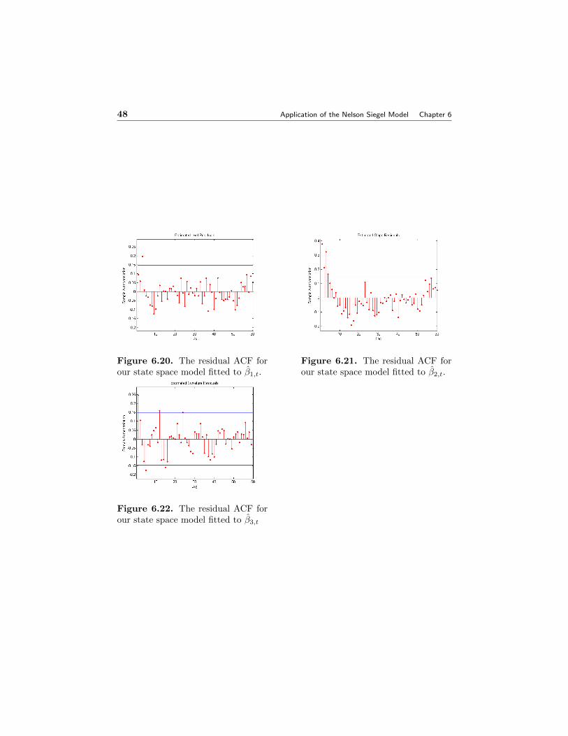
48 Application of the Nelson Siegel Model Chapter 6

Figure 6.20. The residual ACF forour state space model fitted to β1,t.

Figure 6.21. The residual ACF forour state space model fitted to β2,t.

Figure 6.22. The residual ACF forour state space model fitted to β3,t

Section 6.6. Conclusion 49

6.6 Conclusion

In this thesis, I have shown that the term structure of Swedish government bondscan be fitted by applying the dynamic representation of the three-factor NelsonSiegel model. This was achieved by applying Diebold and Li (2006) two step ap-proach, where the model factors, i.e the level, the slope and the curvature, were firstestimated using ordinary least squares and thereafter model as stable independentAR(1) processes. I have therefore shown that the, with only three unknown param-eters, the two-step approach can be used to estimate the term structure of Swedishgovernment bonds. The estimates gave a good in-sample fit for short maturities butthey display difficulties in fitting Swedish government bonds with long maturitiesand at dates where the term structure exhibits multiple minima/maxima.

I therefore instead to further study how these drawbacks can be improve uponin a masters thesis. I intend to follow Svensson (1997) and extend the three-factor model by adding a second curvature in the model. I also intend to usedboth the three-factor model and the Svensson extension to predict and forecast theterm structure of Swedish government bonds. The performance of these models in-sample and out-sample fit will be contrasted. I also intend to lift the arbitrage-freeassumption made on the Swedish government bonds throughout this thesis.

BIBLIOGRAPHY

[1] Interest Rate Models, Theory and Practice, Damiano Brigo and Fabio Mercurio,August 2001.

[2] Time Series Analysis, Henrik Madsen .

[3] Arbitrage Theory in Continuous Time, Bjork 3th Edition.

[4] Finance Market,Instruments and Investments, Hans Bystrom, 2nd Edition.

[5] Modeling Non-Linear and Non-Stationary Time Series, Hendrik Madsen and JanHolst, December 2000.

[6] Stationary Stochastic Processes,Georg Lindgren, Holger Rootzen and Maria Sand-sten, September 2009.

[7] Derivative Pricing part I and II, Sebastian Aberg, 2010.

[8] Rantebarande Instrument, Vardering och Riskhantering, Hossien Asgharian andLars Norden.

[9] De Finansiella Marknaderna i ett Internationellt Perspektiv, Leif Hassel, MarieNorman and Christian Andersson .

[10] Estimating Forward Interest Rates with the Extended Nelson and Siegel Mothod,Lars E.O. Svensson, (1994).

[11] Interest Rate Dynamics and Consistent Forward Rate Curves. Bjork T. andChristensen B. J. (1999).

[12] Forecasting the term structure of government bond yields, Francis X. Dieboldand Canlin Li, (2006) .

[13] Estimating the Yield Curve Using the Nelson-Siegel Model, A Ridge RegressionApproach, Jan Annaert, Anouk G.P Claes, Marc J.K De Ceuster, Hairui Zhand,2000.

50

Bibliography 51

[14] An Arbitrage-Free Generalized Nelson-Siegel Term Structure Model, Jens H.E.Christensen, Francis X. Diebold, Glen D. Rudebusch, November 2008.

[15] Calibrating the Nelson-Siegel-Svensson model, M. Gilli, Stefan Grobe andE.Schumann. march 2010.

[16] Examining the Nelson-Siegel Class of Term Structure Models, Michiel DePooter, June 2007.