The Term Structure of Commercial Paper Rates

Chris Downing and Stephen Oliner∗

Federal Reserve BoardApril 2, 2004

Abstract

This paper tests the expectations hypothesis in the market for commercial paper.

Our main dataset, which is new to the literature, consists of daily indexes constructed

from the actual market yields for nearly all commercial paper issued by U.S. corpora-

tions between January 1998 and August 2003. We show that the term premia built

into commercial paper yields rise dramatically at year-end, causing the expectations

hypothesis to be rejected. However, once we control for these predictable year-end

effects, we find the reverse—that commercial paper yields largely conform with the

expectations hypothesis.

Key words: Term structure; Expectations hypothesis; Commercial paperClassification: E43

This paper has benefited from discussions with Geert Bekaert, Jim Clouse, Francis Longstaff, and BrianSack; the authors thank Jonathan Wright for useful econometric advice and for providing computer code tocalculate robust confidence intervals; all errors and omissions remain the responsibility of the authors. Theviews expressed are those of the authors and should not be attributed to the Board of Governors of the FederalReserve System or its staff. Please address correspondence to (Downing): Federal Reserve Board, Mail Stop93, Washington, DC 20551. Phone: (202) 452-2378. Fax: (202) 728-5887. E-Mail: cdowning@frb.gov.(Oliner): Federal Reserve Board, Mail Stop 66, Washington, DC 20551. Phone: (202) 452-3134. Fax: (202)452-5296. E-Mail: soliner@frb.gov.

1 Introduction

Interest in the expectations hypothesis of the term structure of interest rates dates back

at least a century, largely because it is rooted in one of the most basic concerns of capital

market participants: Is one better off committing funds for a long or short period? Tests of

the expectations hypothesis also command attention because they shed light on the formation

of expectations, the operation of financial markets, and the transmission of monetary policy

through the markets.

Accordingly, an enormous amount of research has been devoted to testing the expecta-

tions hypothesis.1 In general, although not uniformly, the expectations hypothesis has been

rejected in various U.S. credit markets.2 Recently, however, Longstaff (2000) found strong

empirical support for the expectations hypothesis in the market for domestic U.S. repurchase

agreements of less than 90 days maturity. Longstaff’s results raise the question of whether

the expectations hypothesis holds in other very short-term U.S. credit markets.

This paper tests the expectations hypothesis in the market for commercial paper. Com-

mercial paper (CP) is an unsecured debt instrument of up to 270 days’ maturity issued by

investment-grade corporations. Firms use CP to finance inventories, to provide bridge fi-

nancing in connection with various transactions, and for day-to-day cash management. The

commercial paper market is large, with approximately $1.3 trillion outstanding at the end of

2003. In the fourth quarter of 2003, daily placements of commercial paper averaged about

$100 billion, principally in maturities of 90 days or less, and each day an average of about

1For surveys of this literature, see Melino (1988) and Shiller (1990); Campbell, Lo and MacKinlay (1996)provide a textbook treatment.

2The empirical evidence from foreign markets has been somewhat more supportive of the expectationshypothesis. See Hardouvelis (1994), Gerlach and Smets (1997), Dahlquist and Jonsson (1995), and Bekaert,Hodrick and Marshall (2001). Gerlach and Smets (1997) suggest that the better performance of the ex-pectations hypothesis in some foreign markets owes to the greater predictability of short rates in thosemarkets.

1

500 firms issued new paper. Despite this active new-issue market, secondary trading is thin,

consisting primarily of trades between the major dealers and investors who wish to liquidate

their holdings.3

In addition to having limited liquidity, commercial paper is subject to default. Hence,

the difference in expected returns between a long-term position in commercial paper and

a strategy of rolling over shorter-term paper will reflect not only the usual premia that

compensate investors for interest-rate risk, but also premia to compensate for default risk.

Testing the expectations hypothesis in the commercial paper market is of interest for

several reasons. First, this test offers additional evidence on the expectations hypothesis for

very short-term interest rates, where only limited research has been conducted.4 Second, as

mentioned above, commercial paper is a defaultable instrument traded in a relatively thin

secondary market. Accordingly, tests of the expectations hypothesis in this market offer

insights into the interaction of default and liquidity risk with the expectations hypothesis.

Third, commercial paper rates are strongly influenced by monetary policy. Hence, our results

have implications for the transmission of monetary policy to private interest rates.5

We conduct our main tests of the expectations hypothesis using a comprehensive database

on commercial paper yields published by the Federal Reserve. This database, which is new to

the literature, consists of daily indexes constructed from the actual market yields on nearly all

commercial paper issued by U.S. firms, beginning in January 1998. Using these transactions-

based data, we show that term premia for commercial paper jump up at year-end, causing the

expectations hypothesis to be rejected. The year-end jump probably reflects a combination

3For further discussion of the commercial paper market, see Stigum (1990).4Besides Longstaff (2000), the only studies we are aware of that have characterized the overnight to 90-

day portion of the yield curve are Simon (1990), Roberds, Runkle and Whiteman (1996), Balduzzi, Bertolaand Foresi (1997), Lange, Sack and Whitesell (2003), and Swanson (2004).

5For recent studies that highlight the role of the expectations hypothesis in the transmission of monetarypolicy, see Rudebusch (1995), Balduzzi et al. (1997), Kozicki and Tinsley (2001), and Roush (2001).

2

of factors. One contributing factor appears to be “window dressing” on the part of some

large institutional investors. Just prior to releasing their year-end financial statements, these

investors evidently have an incentive to temporarily substitute Treasury bills and other safe

instruments for their holdings of commercial paper—especially lower-grade paper—to present

a strong balance sheet to investors.6 Another likely factor is the desire of commercial paper

issuers to lock-in longer-term funding over year-end when conditions in overnight markets

tend to be volatile. Their willingness to pay a premium for this insurance boosts the yield

on longer-term commercial paper at year-end.

We then test whether the expectations hypothesis holds after controlling for these pre-

dictable year-end effects. The key result of the paper is that, with these controls in place, we

find strong support for the expectations hypothesis in the commercial paper market. Evi-

dently, the term premia in commercial paper yields are fairly stable other than at year-end.7

For completeness, we also conduct the same tests with daily yield indexes constructed

from dealer quotes spanning March 1989 to August 1997. Although these indexes served

as the Federal Reserve’s official series on commercial paper yields until 1997, they are less

accurate than the indexes based on actual transactions, and the Fed stopped publishing

the dealer quotes when the transaction data became available. In contrast to the transac-

tions data, the yields based on dealer quotes reject the expectations hypothesis, even after

controlling for year-end effects.

One possible explanation for the different results is that the dealer-quote data are of

6This argument requires that demand for commercial paper be inelastic, so that other investors do not fillthe void at prevailing yields. See Musto (1997) and Musto (1999) for additional discussions of the windowdressing hypothesis.

7The days following the terrorist attacks of September 11, 2001 are a notable exception. The attacksseverely disrupted the operation of the commercial paper market, an unanticipated event that producedsharp movements in realized term premia. We treat these observations as outliers to prevent them fromaffecting our conclusions.

3

inferior quality—perhaps containing stale quotes, for example—and do not accurately reflect

the dynamics of commercial paper rates. An alternative explanation relates to the conduct

of monetary policy. As documented by Lange et al. (2003) and Swanson (2004), the Federal

Open Market Committee (FOMC) has taken many steps since the late 1980s to make its

views on the economy and its policy actions more transparent. Among these steps, the

FOMC began in February 1994 to announce policy changes on the day of its meetings and

to explain the reasons for the change. Likely reflecting the greater transparency of monetary

policy, Lange et al. found that the federal funds rate became more predictable starting in

1994 and that the expectations hypothesis performed far better after that point than in

earlier years.8 We obtain similar results when we split the dealer-quote data for CP rates at

February 1994: the earlier data soundly reject the expectations hypothesis, but we find more

support for the hypothesis from 1994 on. This finding suggests that the later period covered

by the transactions data (1998-2003) may help explain the differing results generated by these

data and the full sample of dealer quotes. If we had a longer history for the transactions

data, we could run a more definitive test of this explanation. However, in the absence of

such a test, we cannot rule out that the inferior quality of the dealer-quote data also plays

a role.

The only previous tests of the expectations hypothesis with commercial paper yields

appear to have been conducted by Fama (1986) and Cook and Hahn (1990), neither of

which dealt with year-end effects. Both studies rejected the expectations hypothesis using

dealer-quote indexes, consistent with our results based on the pre-1994 dealer-quote data.

This paper is organized as follows. In section 2, we review the theory of the expectations

8Swanson (2004) finds some deterioration in the predictability of the federal funds rate since 2001. How-ever, for the period since 1994 as a whole, he concludes that increased predictability remains a robustfeature of the data and that changes in FOMC transparency have likely helped to make the funds rate morepredictable.

4

hypothesis and our specification of time-varying term premia. Section 3 discusses our data

and econometric results, and section 4 concludes with some final thoughts on the implications

of our results and some directions for future work.

2 Theory

2.1 The Expectations Hypothesis

Denote by r(m, t) the interest rate at time t on a spot loan to be repaid at time t + m (a

discount bond of maturity m). Similarly, let f(m, t + i, t) denote the interest rate at time t

on a forward loan that starts at time t + i and ends at time t + i + m. We measure both

r(m, t) and f(m, t + i, t) on a continuously compounded and annualized basis. Using m = 1

to denote an overnight maturity, we can write the following relationships between forward

overnight rates and future spot overnight rates:

f(1, t + 0, t) − r(1, t) = 0 (1)

f(1, t + 1, t) − r(1, t + 1) = νt+1 (2)

f(1, t + 2, t) − r(1, t + 2) = νt+2 (3)

...

f(1, t + m − 1, t) − r(1, t + m − 1) = νt+m−1 (4)

where the ν· are random errors. Equation 1 states that, by definition, the forward overnight

rate zero days ahead equals the current spot overnight rate. Equations 2-4 state that the

forward overnight rate set at time t for time t + i (i = 1, 2, . . . , m − 1) will differ from the

5

spot overnight rate realized at time t + i by the random amount νt+i.

To develop a test of the expectations hypothesis, we first add the elements on each side

of equations 1-4, producing:

t+m−1∑i=t

(f(1, i, t) − r(1, i)) =t+m−1∑i=t+1

νi. (5)

Noting that the m-period continuously-compounded spot rate r(m, t) equals the average of

the forward overnight rates over its term (r(m, t) = 1m

t+m−1∑i=t

f(1, i, t)), we have:

r(m, t)m =t+m−1∑

i=t

r(1, i) +t+m−1∑i=t+1

νi. (6)

Next, multiply equation 6 by 1m

, subtract r(1, t) from both sides, and rearrange terms,

producing:

1

m

t+m−1∑i=t

r(1, i) − r(1, t) = (r(m, t) − r(1, t)) − 1

m

t+m−1∑i=t+1

νi. (7)

Now introduce β∗m = 1, and write

t+m−1∑i=t+1

νi as the sum of a predictable component, α∗m,t,

and a mean-zero error term, ε∗m,t, which produces:

1

m

t+m−1∑i=t

r(1, i) − r(1, t) = − 1

mα∗

m,t + β∗m (r(m, t) − r(1, t)) − 1

mε∗m,t. (8)

Equation 8 can be rewritten in the following equivalent but more convenient form that we

use for our regression tests:

r(m, t) − 1

m

t+m−1∑i=t

r(1, i) = αm,t + βm(r(m, t) − r(1, t)) + εm,t, (9)

6

where αm,t ≡ 1m

α∗m,t, βm ≡ 1 − β∗

m, and εm,t ≡ 1m

ε∗m,t. Under rational expectations, εm,t

is uncorrelated with information available at time t, including the yields appearing on the

right-hand side of equation 9. As a result, the αm,t and βm coefficients can be estimated

consistently with ordinary least squares.

The expectations hypothesis rules out any time variation in term premia.9 In terms of the

coefficients in equation 9, we characterize the expectations hypothesis with the restrictions

αm,t = αm, a time-invariant constant for each maturity m, and βm = 0 for all m. The

so-called pure expectations hypothesis further requires that αm = 0. In other words, under

the expectations hypothesis, the difference between an m-period yield and the average of

the overnight yields over the same period equals a constant, possibly equal to zero, plus

expectational error.

2.2 Year-End Premia in the Commercial Paper Market

Predictable year-end effects are a key component of term premia at all maturities in the

commercial paper market. We illustrate these effects for the 30-day maturity in figure 1;

the other maturities exhibit qualitatively similar year-end effects and so are omitted for

the sake of brevity. Panel A of the figure shows 30-day term premia for CP issued by the

highest quality firms—those with short-term credit ratings of A1/P1 and long-term bond

ratings of AA or better.10 The term premia are computed as the difference between the

30-day CP rate and the average overnight CP rate over the same 30-day period. The panel

9Many different versions of the expectations hypothesis have appeared in the literature. At longer matu-rities, some forms of the expectations hypothesis are inconsistent with each other. However, for maturitiesas short as we consider here, the various forms of the expectations hypothesis are virtually the same (seeLongstaff (2000) for further discussion).

10Standard and Poor’s and Moody’s both issue short-term ratings on a three-point scale (1, 2, and 3),with 1 being the highest and 3 being the lowest. Standard and Poor’s prefixes their short-term ratings withan ’A’, while Moody’s uses a ’P’. Thus, an A1/P1 rating means that the firm received a ’1’ rating by bothrating agencies.

7

displays both the dealer-quote data (1989-1997) and the transaction-based data (1998-2003)

that we discuss at length in section 3.1 below.11 Panel B shows 30-day term premia for CP

issued by A2/P2-rated firms with long-term bond ratings of BBB or A—issuers with credit

quality substantially below those in the upper panel; this series begins in 1998 because the

dealer-quote data for this rating class are very limited. As can be seen, the 30-day term

premium tends to jump as year-end approaches, with the largest increases for A2/P2-rated

issuers. This additional premium then disappears as soon as year-end passes. The size of

the spike varies from year to year, and we allow for this variation in our empirical tests of

the expectations hypothesis. In recent years, the largest jump occurred in advance of the

century date change at the end of 1999.

Year-end effects in other money markets are more muted, on balance, than those in the

commercial paper market. For example, as shown in figure 2, term premia do tend to rise

at year-end in the markets for repurchase agreements (panel A) and federal funds (panel

B). However, for repurchase agreements (“repo”), the year-end increases are relatively small

and are often difficult to distinguish from the variation throughout the rest of the year. For

federal funds, the year-end increases in the term premium are roughly on par with those

for AA-rated commercial paper but are much smaller than the spikes observed for A2/P2

paper. These differences likely help to explain why Longstaff (2000) could not reject the

expectations hypothesis in the repo market even without controls for year-end effects and

why Lange et al. (2003) found that the expectations hypothesis has performed reasonably

well in the federal funds market since the early 1990s, again without year-end controls.

Year-end effects are evident as well in the quantity of commercial paper outstanding.

11The break in the series reflects the Fed’s switch from dealer quotes to the transactions data. Although30-day rates based on the transactions data are available back to the beginning of 1997, the series forovernight rates starts a year later, which prevents us from using the 1997 data.

8

Figure 3 displays the level of outstanding commercial paper for “tier-1” and “tier-2” issuers.12

The lower panel indicates that CP outstanding for tier-2 issuers declines systematically at

year-end and that the drop is usually reversed in January. This pattern is much less evident

for tier-1 issuers, further indicating that year-end effects are concentrated among lower-

quality firms.

Another notable feature of the CP market is that the volume of maturing paper declines

markedly at year-end. Figure 4 illustrates this point by showing the average maturity struc-

ture of outstanding commercial paper at two points in December–the first Wednesday of the

month (panel A) and the third Wednesday (panel B). The bars depict the average amount

of paper, as of the indicated date, that is set to mature in the maturity ranges shown on

the horizontal axis. The dotted vertical lines indicate year-end, and the solid lines indicate

the average maturity structure for all other Wednesdays.13 The distributions of outstand-

ing paper reveal a pronounced drop in the amount of paper maturing around year-end. As

year-end approaches, the maturity structure tends to shift toward longer-dated paper, with

the amount of CP maturing after year-end being substantially greater than would be pre-

dicted by the average maturity structure of paper at other times of the year. This paucity

of maturing paper, combined with the limited amount of secondary market trading, points

to a fall-off in market liquidity at year-end.

One explanation for these year-end patterns focuses on “window dressing” by some in-

12Rule 2a-7 of the Investment Company Act of 1940 limits the credit risk that money market mutual fundsmay bear by restricting their investments to “eligible” securities. An eligible security must carry one of thetwo highest ratings (“1” or “2”) for short-term obligations from at least two of the nationally recognizedstatistical ratings agencies (which currently consist of Standard and Poor’s, Moody’s, and Fitch IBCA). Atier-1 security is an eligible security rated “1” by at least two of the rating agencies; a tier-2 security is aneligible security that is not a tier-1 security. We employ this quality split in order to display lengthy timeseries, as the Federal Reserve data provide only a limited history for CP outstanding based on the A1/P1versus A2/P2 split.

13We use Wednesdays for the figure because the Federal Reserve releases its data on CP outstanding at aweekly-Wednesday frequency.

9

vestors in the commercial paper market (Musto (1997, 1999)). According to the Federal

Reserve’s Flows of Funds accounts, approximately one-half of all outstanding commercial

paper is held by money market mutual funds, insurance companies, and pension funds.

Most of these entities report on their portfolio holdings at year-end, and they show some

propensity to window dress their balance sheets by temporarily substituting higher-quality

investments for their usual holdings. Given this behavior, lower-quality issuers likely would

have to offer a yield premium to induce investors to hold their paper over year-end. Rather

than paying such a premium, some issuers might find it less costly to turn to other forms of

finance at year-end, which would help explain the drop in outstanding paper.14

A second explanation focuses on uncertainty in short-term financing markets at year-end.

Overnight interest rates tend to be highly volatile at that time of year because of the large—

and variable—increases in demand for cash by financial institutions, nonfinancial businesses,

and individuals. Figure 5 depicts one measure of this heightened rate volatility. As shown,

the deviation of the federal funds rate from its target tends to be substantially larger around

year-end than during the rest of the year. To the extent that this volatility is transmitted to

other very short-term instruments like overnight commercial paper, firms might be willing to

insure against this interest-rate risk by issuing longer-maturity paper in lieu of rolling over

paper every day. The spike in term premia around year-end shown in figure 1 could partly

reflect the price that issuers are willing to pay for this insurance.

14Window dressing by money fund managers might also help explain the year-end pricing effects observedin the Treasury bill market. If enough CP investors move their funds into Treasury bills for a short timearound year-end, this flow could cause the temporary increase in Treasury bill prices documented by Duffee(1996).

10

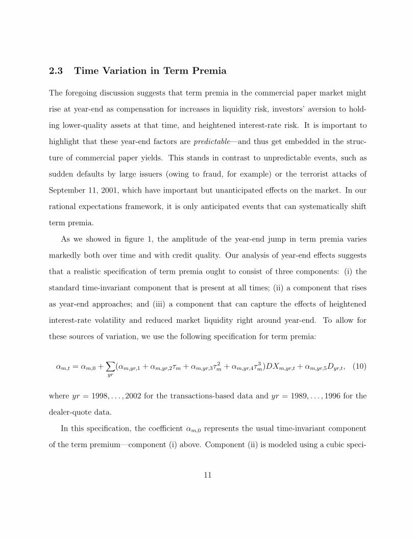
2.3 Time Variation in Term Premia

The foregoing discussion suggests that term premia in the commercial paper market might

rise at year-end as compensation for increases in liquidity risk, investors’ aversion to hold-

ing lower-quality assets at that time, and heightened interest-rate risk. It is important to

highlight that these year-end factors are predictable—and thus get embedded in the struc-

ture of commercial paper yields. This stands in contrast to unpredictable events, such as

sudden defaults by large issuers (owing to fraud, for example) or the terrorist attacks of

September 11, 2001, which have important but unanticipated effects on the market. In our

rational expectations framework, it is only anticipated events that can systematically shift

term premia.

As we showed in figure 1, the amplitude of the year-end jump in term premia varies

markedly both over time and with credit quality. Our analysis of year-end effects suggests

that a realistic specification of term premia ought to consist of three components: (i) the

standard time-invariant component that is present at all times; (ii) a component that rises

as year-end approaches; and (iii) a component that can capture the effects of heightened

interest-rate volatility and reduced market liquidity right around year-end. To allow for

these sources of variation, we use the following specification for term premia:

αm,t = αm,0 +∑yr

(αm,yr,1 + αm,yr,2τm + αm,yr,3τ2m + αm,yr,4τ

3m)DXm,yr,t + αm,yr,5Dyr,t, (10)

where yr = 1998, . . . , 2002 for the transactions-based data and yr = 1989, . . . , 1996 for the

dealer-quote data.

In this specification, the coefficient αm,0 represents the usual time-invariant component

of the term premium—component (i) above. Component (ii) is modeled using a cubic speci-

11

fication in time that is in effect only near year-end. Specifically, the variable DXm,yr,t equals

one when the observation date t is before, and the maturity date t + m is after, December

26 of the year indexed by yr. We allow DXm,yr,t to switch on for maturities slightly before

year-end because figure 4 suggests that year-end effects begin to be seen about a week before

the turn of the year. When this dummy variable equals one, the variable τm counts the

number of days from December 26 of the given year to the maturity date t + m. The cubic

term in τ allows the specification to capture a wide range of time patterns for the year-end

term premium. Finally, component (iii) is modeled with the dummy variable Dyr,t, which

equals one when the observation date t is between December 22 of the year indexed by yr

and January 10 of the following year. Hence the coefficient αm,5 captures any level shifts in

term premia right around year-end, when, as we discussed earlier, liquidity in the market

appears low and short-term interest rates are relatively volatile. Allowing the coefficients to

vary across years introduces additional flexibility. In the next section, we test traditional

specifications of term premia, as well as our new specification that incorporates year-end

premia.

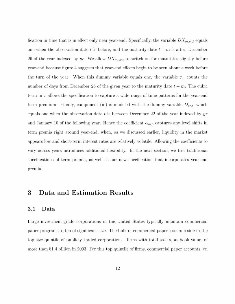
3 Data and Estimation Results

3.1 Data

Large investment-grade corporations in the United States typically maintain commercial

paper programs, often of significant size. The bulk of commercial paper issuers reside in the

top size quintile of publicly traded corporations—firms with total assets, at book value, of

more than $1.4 billion in 2003. For this top quintile of firms, commercial paper accounts, on

12

average, for 30 percent of their current liabilities, making it an important source of short-term

credit.15

We employ two sources of daily data on commercial paper yields.16 Our primary source

consists of the commercial paper discount yields currently published by the Federal Reserve

Board for AA-rated and A2/P2-rated domestic nonfinancial companies. We focus on ma-

turities of 90 days or less because the market for longer-maturity paper is quite thin. The

Federal Reserve Board constructs these yield indexes from transaction-level data supplied by

the Depository Trust Company, which handles clearing and settlement for more than 95 per-

cent of all commercial paper trades in the United States. Federal Reserve staff fit a smooth

curve to the transaction-level data. The end result is a daily series of constant-maturity,

zero-coupon yields.17 Our yield data cover each business day from January 2, 1998 through

August 1, 2003, for a total of 1,365 daily observations.

The upper two panels of table 1 display summary statistics for these transactions-based

yields. For AA-rated issuers (top panel), yields rise very little with increases in maturity,

resulting in a mean spread between 90-day and overnight paper of only 3.09 basis points.

In contrast, for A2/P2-rated issuers (middle panel), the mean 90-day spread is 19.09 basis

points, reflecting the greater default and liquidity risks in this part of the market. The yields

for both AA and A2/P2 paper are highly autocorrelated at all maturities, consistent with

the behavior of other short-term interest rates.

We also make use of a second database, consisting of dealer quotes on yields for com-

15These figures are calculated using the Federal Reserve’s commercial paper database and Compustat.16The yield indices used to construct the term premia are from the Federal Reserve’s daily commercial

paper release. Details can be found at:http://www.federalreserve.gov/Releases/cp/about.htm.

17This procedure does not have to deal with the effect of coupons on observed yields because the underlyingdata pertain to newly-issued discount instruments. Thus, the smoothing procedure directly estimates thediscount function itself, as opposed to extracting the discount function implied by the prices of couponsecurities.

13

mercial paper issued by a generic AA-rated domestic corporation, collected by the Federal

Reserve Bank of New York between February 27, 1989 and August 29, 1997.18 Over this

period, the New York Fed surveyed the major dealers each day and constructed unweighted

averages of the rates reported for various maturities. The lower panel of table 1 displays

summary statistics for these data. As shown, the longer-term yields from the dealer survey

exhibit higher spreads to overnight rates than the transactions-based AA yields, reaching

14.59 basis points at the 90-day maturity. One possible explanation for the higher spreads

is that, while the dealers were instructed to report yields for AA-rated corporations, they

may have in fact provided yields for firms of lesser credit quality.19

3.2 A First Look at Term Premia

To characterize term premia in the commercial paper market, table 2 reports estimates of

the following regression:

r(m, t) − 1

m

t+m−1∑i=t

r(1, i) = αm + εm,t, (11)

where αm represents the average term premium at maturity horizon m, and εm,t is a mean-

zero error term. Recalling equation 9, this specification imposes the restrictions from the

expectations hypothesis—namely, that αm,t is time-invariant and that βm equals zero—and

then estimates the average term premium conditional on these restrictions.

As shown in the upper two panels of the table, the transactions data clearly indicate

that term premia are non-zero, with the exception of the shortest maturity (7 days) for the

18The New York Fed surveyed dealers going back to the 1960s, but only for a limited range of maturities.In order to make our results comparable across the two sources of data, we restrict our analysis of thedealer-quote data to the period over which the dealer survey included the widest range of maturities.

19See Cook and Lawler (1983) for further discussion of the New York Fed’s dealer survey.

14

highest-quality issuers. On average, AA-rated issuers pay 3.50 basis points more to place

30-day paper than to roll overnight paper for 30 days, while A2/P2-rated issuers pay 12.76

basis points more; over a 90-day horizon, these premia rise to 11.93 basis points for AA

issuers and 27.85 basis points for A2/P2 issuers.20 Based on these results, we would clearly

reject the pure expectations hypothesis in the commercial paper market.

The dealer-quote data support a similar conclusion. The estimates of term premia in

the lower panel are highly significant and larger in size than those based on the transactions

data for AA firms, the part of the market to which the quotes should apply. In fact, for

every maturity, the estimated term premium is closer to the premium for A2/P2-rated firms

than to that for AA-rated firms.

3.3 Tests of the Expectations Hypothesis

3.3.1 Maturity-Specific Term Premia

We first consider the evidence for the standard version of the expectations hypothesis that

allows term premia to vary by maturity but not over time:

r(m, t) − 1

m

t+m−1∑i=t

r(1, i) = αm + βm (r(m, t) − r(1, t)) + εm,t. (12)

In contrast to equation 11, this specification tests whether βm = 0 rather than imposing

that restriction a priori. Table 3 displays the estimates of αm and βm, along with their

t-statistics. The t-statistics are corrected for the overlap in the errors. However, as is well

known in the term structure literature, interest rates are highly persistent, a feature that

20These results contrast with those in Longstaff (2000), who found a 90-day term premium of just 3 basispoints using data on repurchase agreements. We would expect term premia to be greater in the commercialpaper market both because repo contracts are almost free of default risk and because these contracts aremore liquid than commercial paper.

15

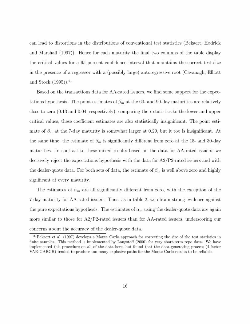
can lead to distortions in the distributions of conventional test statistics (Bekaert, Hodrick

and Marshall (1997)). Hence for each maturity the final two columns of the table display

the critical values for a 95 percent confidence interval that maintains the correct test size

in the presence of a regressor with a (possibly large) autoregressive root (Cavanagh, Elliott

and Stock (1995)).21

Based on the transactions data for AA-rated issuers, we find some support for the expec-

tations hypothesis. The point estimates of βm at the 60- and 90-day maturities are relatively

close to zero (0.13 and 0.04, respectively); comparing the t-statistics to the lower and upper

critical values, these coefficient estimates are also statistically insignificant. The point esti-

mate of βm at the 7-day maturity is somewhat larger at 0.29, but it too is insignificant. At

the same time, the estimate of βm is significantly different from zero at the 15- and 30-day

maturities. In contrast to these mixed results based on the data for AA-rated issuers, we

decisively reject the expectations hypothesis with the data for A2/P2-rated issuers and with

the dealer-quote data. For both sets of data, the estimate of βm is well above zero and highly

significant at every maturity.

The estimates of αm are all significantly different from zero, with the exception of the

7-day maturity for AA-rated issuers. Thus, as in table 2, we obtain strong evidence against

the pure expectations hypothesis. The estimates of αm using the dealer-quote data are again

more similar to those for A2/P2-rated issuers than for AA-rated issuers, underscoring our

concerns about the accuracy of the dealer-quote data.

21Bekaert et al. (1997) develops a Monte Carlo approach for correcting the size of the test statistics infinite samples. This method is implemented by Longstaff (2000) for very short-term repo data. We haveimplemented this procedure on all of the data here, but found that the data generating process (4-factorVAR-GARCH) tended to produce too many explosive paths for the Monte Carlo results to be reliable.

16

3.3.2 Controlling for Time Variation in Term Premia

We now consider the evidence for the expectations hypothesis after we control for the rise in

term premia around year-end and for the idiosyncratic effects of the September 11 terrorist

attacks. In this case, our specification is given by:

r(m, t) − 1m

t+m−1∑i=t

r(1, i) = αm,0 + βm(r(m, t) − r(1, t))+

∑yr

(αm,yr,1 + αm,yr,2τm + αm,yr,3τ2m + αm,yr,4τ

3m)DXm,yr,t + αm,yr,5Dyr,t +

αm,6SXm,t + αm,7St + εm,t.

(13)

For the transaction data, yr = 1998, . . . , 2002, while for the dealer-quote data, yr =

1989, . . . , 1996. The variables DXm,yr,t, Dyr,t, and τm are as defined in section 2.3, and

SXm,t and St are variables designed to control for the effects of the September 11 attacks on

the CP market.

These attacks severely disrupted the computer networks that money-market participants

rely on to carry out their transactions. With some banks unable to transfer the funds

necessary to redeem maturing commercial paper, a sizable portion of the paper that came

due in the days following the attacks could not be honored.22 Moreover, a large number of

issuers could not roll over maturing paper. Many of these issuers instructed their banks to

draw down liquidity backup lines in order to make payments on maturing paper, producing

substantial draws at the discount window at the Fed.23

These market disruptions produced significant pricing effects in the commercial paper

22The situation was analagous to an individual attempting to cash a check, and upon finding the necessaryfunds unavailable, returning the next day to try again. In the jargon of the money markets, the maturitypresentments were “failed” and presented again the next day.

23For a full description of the Federal Reserve’s response to the stresses in the U.S. financial system, seethe Monetary Report to Congress, February 2002, available at:http://www.federalreserve.gov/boarddocs/hh/2002/February/FullReport.htm.

17

market. Yields on the Tuesday of the attacks showed little change from Monday, but they

likely reflected pricing on deals done in the morning before the attacks.24 On Wednesday,

yields on overnight paper jumped about 30 basis points for AA-rated issuers, and about

60 basis points for A2/P2 issuers.25 Overnight yields rose further on Thursday and Friday,

as operational risks in the clearance and settlement systems remained significant, raising

the possibility of defaults. Then, on the Monday following the attacks, yields dropped

precipitously, owing in part to a 50 basis point cut in the target federal funds rate just prior

to the reopening of the equity markets, as well as to the sizable liquidity injections by the

Fed in the days following the attacks. Rates continued to gyrate for the remainder of the

month, but by the beginning of October, the market had largely stabilized.

To account for these effects, we introduce the dummy variable SXm,t which takes the

value one when the observation date t is before September 11, 2001 and the maturity date

t + m is after September 11. When SXm,t equals one, the yields at date t were unaffected

by September 11, but all of the overnight yields realized after September 11—which we use

to construct term premia—were highly elevated. We also introduce the variable St, which

equals one when the observation date t is between September 11 and September 18, 2001, a

period during which all maturities—including overnight paper—bore the imprint of Septem-

ber 11. We treat the observations that are dummied out in this way as outliers resulting

from a singular event that ought not influence our conclusions regarding the expectations

hypothesis.26

24The commercial paper market is a “morning market” in the sense that nearly all of the deals arecompleted before noon, in order to facilitate same-day settlement.

25The Fed’s calculation of yields on these days was hampered by the sharp drop in market liquidity, andthe figures cited here should be regarded as merely indicative.

26While these September 11 dummy variables are similar in their construction to the year-end dummyvariables we introduced earlier, their interpretation is very different. Whereas the year-end dummies controlfor the influence of predictable events on term premia, the September 11 dummy variables are being used toremove the influence of an unpredictable one-time event during the period covered by our transactions data.

18

Table 4 presents the estimates of the αm,0 and βm coefficients in equation 13; the tables

in appendix A.2 display the estimates of all of the year-end and September 11 coefficients.

Based on the transactions data, we find strong support for the expectations hypothesis once

we control for year-end effects and September 11.27 For AA-rated commercial paper, the

point estimates of βm are now much closer to zero than they were absent these controls

(except for 90-day paper, for which βm was already close to zero). Moreover, comparing the

t-statistics to the robust critical values in the last two columns of the table, we see that all

of the slope coefficient estimates are statistically insignificant. For A2/P2-rated commercial

paper, we find that the point estimates of βm are also in the neighborhood of zero. Only the

estimate at the 30-day maturity is statistically significant.

The results for the dealer-quote data, shown in the bottom panel of the table, provide

much less support for the expectations hypothesis. The point estimates of βm shrink in

size after controlling for year-end effects, but they remain statistically significant except at

the 7-day maturity. In addition, these coefficient estimates are generally larger than those

obtained with the transactions data.

As noted earlier, year-end changes in term premia are a dominant characteristic of com-

mercial paper yields. Table 5 quantifies this fact by comparing the adjusted-R2 statistics

from the standard regression (equation 12) with those from the specification that accounts

for year-end effects and September 11 effects (equation 13). In every case, the R2 rises dra-

matically with the inclusion of these controls. Indeed, for the 90-day AA-rated transaction

data, the R2 rises from essentially zero to nearly 60 percent, and most of the other table

entries show a jump of at least 30 percentage points.28

27If we omit the September 11 dummy variables, our qualitative results are unchanged, but some coefficientsare less precisely estimated.

28In every regression, the September 11 dummy variables account for only a small part of the increase inR2. For the AA-rated data, the September 11 dummy variables contribute between three and 14 percentage

19

3.3.3 Year-End and September 11 Effects

Recall that equation 13 includes a cubic polynomial function to capture the movements in

term premia as year-end approaches. Figures 6 and 7 plot this estimated function for 30-

day commercial paper yields.29 As shown in figure 6, using the transactions-based data, we

find that term premia for both AA- and A2/P2-rated issuers vary considerably from year

to year. However, more often than not, the term premia display a concave pattern, initially

rising and then declining as the issue date approaches year-end. This pattern was especially

pronounced in 1999, just ahead of the century date change. In that year, term premia initially

shot up on concerns that computer bugs could hinder the functioning of financial markets

but plummeted shortly before the turn of the year, at least in part because the Federal

Reserve committed to provide substantial liquidity in the event of a market disruption. In

contrast to 1999, year-end premia were muted in some other years, notably for AA-rated

issuers in 2001 and 2002. The year-to-year variation shown in figure 6 is highly significant:

Using a standard F -test, the null hypothesis that the year-end coefficients are equal across

the years is rejected with more than 95 percent confidence for both rating classes.

Figure 7 displays the analogous estimates for the dealer-quote data. The pattern of year-

end term premia again varies across years. In 1990—a recession year—term premia kept

rising as year-end approached, reaching an extremely high level. However, in 1992, 1993,

and 1994, term premia peaked well before year-end, and in 1995, they were consistently

small. As with the transactions data, an F -test indicates that these differences are highly

points to the increase in R2, while for the A2/P2 data, these controls contribute between one and sixpercentage points.

29These plots are based on the estimates of α30,yr,1, . . . , α30,yr,4 shown in tables A.1-A.3 in appendix A.2.The bulk of the estimated coefficients are statistically significant; thus, we can reject the hypothesis that theplots in each panel equal a horizontal line drawn at zero. To conserve space, we focus here on the 30-daymaturity; the qualitative features of the estimates for the other maturities are similar.

20

significant.

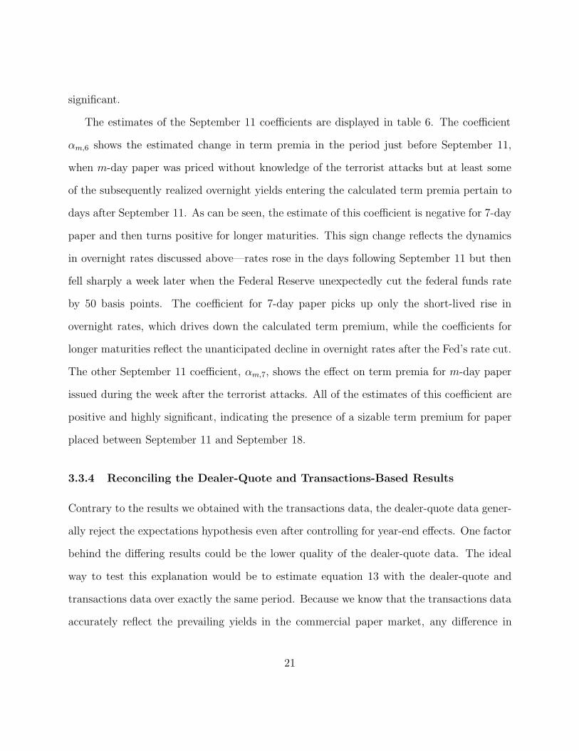
The estimates of the September 11 coefficients are displayed in table 6. The coefficient

αm,6 shows the estimated change in term premia in the period just before September 11,

when m-day paper was priced without knowledge of the terrorist attacks but at least some

of the subsequently realized overnight yields entering the calculated term premia pertain to

days after September 11. As can be seen, the estimate of this coefficient is negative for 7-day

paper and then turns positive for longer maturities. This sign change reflects the dynamics

in overnight rates discussed above—rates rose in the days following September 11 but then

fell sharply a week later when the Federal Reserve unexpectedly cut the federal funds rate

by 50 basis points. The coefficient for 7-day paper picks up only the short-lived rise in

overnight rates, which drives down the calculated term premium, while the coefficients for

longer maturities reflect the unanticipated decline in overnight rates after the Fed’s rate cut.

The other September 11 coefficient, αm,7, shows the effect on term premia for m-day paper

issued during the week after the terrorist attacks. All of the estimates of this coefficient are

positive and highly significant, indicating the presence of a sizable term premium for paper

placed between September 11 and September 18.

3.3.4 Reconciling the Dealer-Quote and Transactions-Based Results

Contrary to the results we obtained with the transactions data, the dealer-quote data gener-

ally reject the expectations hypothesis even after controlling for year-end effects. One factor

behind the differing results could be the lower quality of the dealer-quote data. The ideal

way to test this explanation would be to estimate equation 13 with the dealer-quote and

transactions data over exactly the same period. Because we know that the transactions data

accurately reflect the prevailing yields in the commercial paper market, any difference in

21

estimation results would have to arise from problems with the dealer quotes. However, the

two datasets have no time periods in common, which prevents us from running this test.

Accordingly, we cannot rule out that differences in data quality help explain the divergent

results.

Nevertheless, we can test an alternative explanation that relates to the conduct of mon-

etary policy. As noted in the introduction, Lange et al. (2003) document that the FOMC

has taken many steps over the past fifteen years to make monetary policy more transparent,

which has enabled market participants to better anticipate policy actions. Indeed, Lange

et al. found that the federal funds rate became much more predictable starting in February

1994, when the FOMC began to announce policy changes and the rationale for these actions

shortly after the conclusion of its meetings. Consistent with the greater predictability of the

funds rate, Lange et al. showed that the expectations hypothesis performed considerably

better in the federal funds market after February 1994 than before.30

These developments in the federal funds market have direct implications for our tests of

the expectations hypothesis in the commercial paper market. As shown in figure 8, both

overnight CP rates (panel A) and longer-term yields (panel B) closely track the FOMC’s

target for the federal funds rate. Thus, we might expect the performance of the expectations

hypothesis in the commercial paper market to have improved over the course of the 1990s, as

it did for federal funds. If that were the case, this pattern could help explain why the more

recent transactions-based data provide far more support for the expectations hypothesis than

do the earlier dealer-quote data.

We examine this argument by splitting our dealer-quote data into two subsamples. The

30The link between the predictability of interest rate changes and the expectations hypothesis is analyzedin depth by Mankiw and Miron (1986); for related work, see Balduzzi et al. (1997), Gerlach and Smets(1997), and Rudebusch (1995).

22

first subsample covers the period from the beginning of the sample to February 4, 1994,

the date of the FOMC meeting that corresponds to the Lange et al. breakpoint; the second

subsample includes the rest of the dealer-quote data. Tables 7 and 8 present the coefficient

estimates from re-running both the standard regression and the specification with year-end

controls on each subsample. For the earlier subsample, the top panel of table 7 shows that

the standard regression decisively rejects the expectations hypothesis, as the estimate of βm

is well above zero and highly significant at every maturity. Adding the year-end controls

does not materially change this conclusion; as shown in the lower panel, the estimates of βm

become smaller but they remain significant at all maturities except seven days.

Turning to table 8, we find somewhat more support for the expectations hypothesis in

the later subsample once we control for year-end effects. As shown in the lower panel of

the table, the estimates of βm at the 7-, 15-, and 30-day maturities are close to zero and

statistically insignificant. The estimates for 60- and 90-day maturities are significant, but

they are much smaller in size than their counterparts in table 7. Overall, these results are

consistent with the view that the greater transparency of monetary policy accounts, at least

in part, for the better performance of the expectations hypothesis in recent years.

4 Conclusion

In this paper, we rigorously tested the expectations hypothesis in the market for commercial

paper. Our tests relied on daily yield indexes constructed by the Federal Reserve Board

from the actual market yields for virtually all commercial paper issued by U.S. corporations.

These transactions-based indexes provide an extremely accurate summary of market yields

from 1998 onward. For completeness, we ran a parallel set of tests on the dealer-quote data

23

that the Federal Reserve published before the transactions data became available; the dealer

quotes are less accurate than the transactions-based indexes, but they span a longer period

and have been used in previous research.

Both datasets reject the traditional specification of the expectations hypothesis that

requires the term premium for a given maturity to be constant over time. This rejection is

not surprising, as term premia typically rise in the commercial paper market at year-end,

especially for lower-rated paper. Some plausible explanations for this year-end effect include

“window dressing” by institutional investors, who hold a substantial amount of commercial

paper, as well as a desire by issuers to insure against volatile interest rates and the attendant

increase in rollover risk around year-end.

After we control for these year-end effects, we find strong support for the expectations hy-

pothesis using the transactions data—the key result in the paper. The dealer-quote data, in

contrast, largely reject the expectations hypothesis even after controlling for year-end effects.

We argued that at least some of this difference likely reflects the increasing predictability of

short-term interest rates over the 1990s, though we cannot rule out that the lower quality of

the dealer-quote data also contribute to this result.

Finally, we should note that we have relied exclusively on composite yield indexes to

carry out these tests. Our results with the transactions-based indexes indicate that the

expectations hypothesis is valid for the “average firm” in the commercial paper market.

However, the extent to which the hypothesis holds for individual firms remains an open

question and would be an important topic for future research.

24

Figure 1: Term Premia for 30-Day Commercial PaperThe figure shows term premia for 30-day commercial paper issued by nonfinancial firms rated AA (panel A)and A2/P2 (panel B). Each daily observation is calculated as the difference between the 30-day rate and theaverage of the overnight rates subsequently realized over the term of the 30-day rate. The data in panel Acover the period from February 27, 1989 to August 1, 2003, with a break from August 30, 1997 to January1, 1998. The data in panel B cover the period from January 2, 1998 to August 1, 2003. The vertical lines inboth panels are drawn at year-end.

Panel A: AA-rated firms

-50

0

50

100

150

200

Bas

is P

oint

s

1989 1990 1991 1992 1993 1994 1995 1996 1997 1998 1999 2000 2001 2002 2003

Panel B: A2/P2-rated firms

-50

0

50

100

150

200

Bas

is P

oint

s

1998 1999 2000 2001 2002 2003

Source: Federal Reserve Board (based on data from the Federal Reserve Bank of New York market surveythrough 1997 and data from the Depository Trust Company after 1997).

25

Figure 2: Term Premia for 30-Day Repurchase Agreements and Federal FundsThe figure shows term premia for 30-day repurchase agreements (panel A) and federal funds (panel B). Eachdaily observation is calculated as the difference between the 30-day rate and the average of the overnightrates subsequently realized over the term of the 30-day rate. The data are daily and cover the period May21, 1991 through August 1, 2003. The vertical lines in both panels are drawn at year-end.

Panel A: Repurchase Agreements

-50

0

50

100

150

200

Bas

is P

oint

s

1991 1992 1993 1994 1995 1996 1997 1998 1999 2000 2001 2002 2003

Panel B: Federal Funds

-50

0

50

100

150

200

Bas

is P

oint

s

1991 1992 1993 1994 1995 1996 1997 1998 1999 2000 2001 2002 2003

Sources: Repurchase agreement data are from Garban International; federal funds data are from the FederalReserve Board.

26

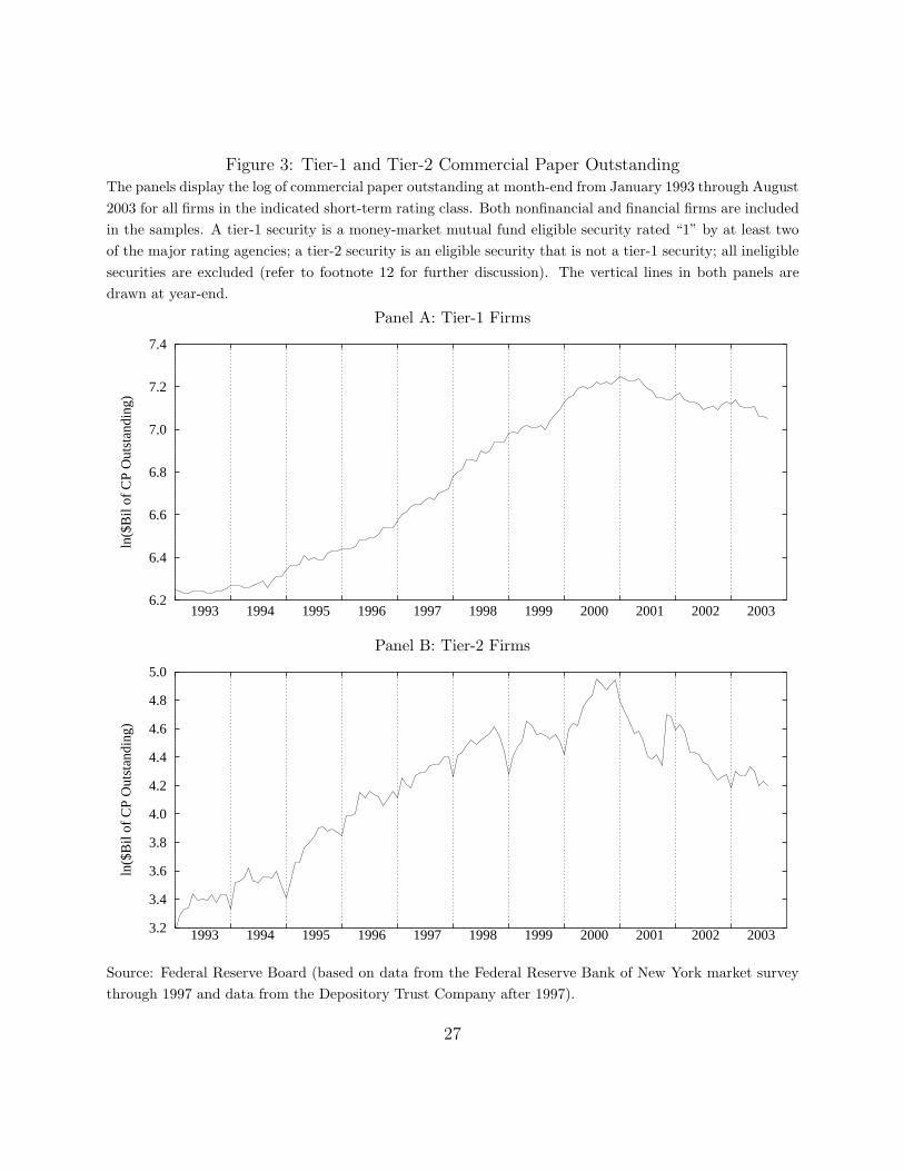
Figure 3: Tier-1 and Tier-2 Commercial Paper OutstandingThe panels display the log of commercial paper outstanding at month-end from January 1993 through August2003 for all firms in the indicated short-term rating class. Both nonfinancial and financial firms are includedin the samples. A tier-1 security is a money-market mutual fund eligible security rated “1” by at least twoof the major rating agencies; a tier-2 security is an eligible security that is not a tier-1 security; all ineligiblesecurities are excluded (refer to footnote 12 for further discussion). The vertical lines in both panels aredrawn at year-end.

Panel A: Tier-1 Firms

6.2

6.4

6.6

6.8

7.0

7.2

7.4

ln($

Bil

of C

P O

utst

andi

ng)

1993 1994 1995 1996 1997 1998 1999 2000 2001 2002 2003

Panel B: Tier-2 Firms

3.2

3.4

3.6

3.8

4.0

4.2

4.4

4.6

4.8

5.0

ln($

Bil

of C

P O

utst

andi

ng)

1993 1994 1995 1996 1997 1998 1999 2000 2001 2002 2003

Source: Federal Reserve Board (based on data from the Federal Reserve Bank of New York market surveythrough 1997 and data from the Depository Trust Company after 1997).

27

Figure 4: Year-End Maturity Structure of Commercial Paper

The figure shows the average amount of nonfinancial and financial commercial paper outstanding that isscheduled to mature in the indicated date ranges. Panel A shows the average amounts outstanding as ofthe first Wednesday of December for all of the years included in the transactions-data sample (1998-2002).Panel B shows the average amounts outstanding as of the third Wednesday in December for the same years.The dotted vertical line in each panel shows the approximate location of December 31. The solid line in eachpanel shows the average maturity structure over all other Wednesdays.

Panel A: First Wednesday of December

0

50

100

150

200

250

300

0-7 15-21 29-35 43-49 57-63 71-77

Bill

ions

of

Dol

lars

Days to Maturity

Panel B: Third Wednesday of December

0

50

100

150

200

250

300

0-7 15-21 29-35 43-49 57-63 71-77

Bill

ions

of

Dol

lars

Days to Maturity

Source: Federal Reserve Board, based on data from the Depository Trust Company.

28

Figure 5: Deviation of Federal Funds Rate from Target

The figure displays the standard deviations of the daily differences of the effective federal funds rate fromthe intended target rate. The solid line shows the standard deviations for year-end observations, defined asobservations after December 25 of the indicated year or before January 5 of the following year. The dashedline displays the standard deviations for all other observations in the indicated year.

0

20

40

60

80

100

120

1989 1990 1991 1992 1993 1994 1995 1996 1997 1998 1999 2000 2001 2002

Bas

is P

oint

s

Year-End Other Days

Source: Federal Reserve Board.

29

Figure 6: Year-End Term Premia for 30-Day Commercial Paper Rates, Transactions Data

The panels plot the cubic portion of the estimated year-end term premium functions for 30-day paper, givenby

α̂m,yr,1 + α̂m,yr,2τm + α̂m,yr,3τ2m + α̂m,yr,4τ

3m

for τ = 0, 1, . . . , 30 and m = 30. When τ = 0, the maturity date is December 26 and when τ = 30 thematurity date is 30 days later (January 24 of the following year). The α̂· denote estimated coefficients fromthe appropriate rows in tables A.1 and A.2.

Panel A: AA-Rated Firms

-20

0

20

40

60

80

100

120

140

0 5 10 15 20 25 30

Bas

is P

oint

s

τ

1998 1999 2000 2001 2002

Panel B: A2/P2-Rated Firms

-20

0

20

40

60

80

100

120

140

0 5 10 15 20 25 30

Bas

is P

oint

s

τ

1998 1999 2000 2001 2002

30

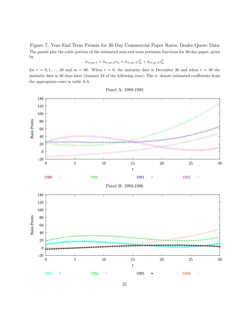
Figure 7: Year-End Term Premia for 30-Day Commercial Paper Rates, Dealer-Quote Data

The panels plot the cubic portion of the estimated year-end term premium functions for 30-day paper, givenby

α̂m,yr,1 + α̂m,yr,2τm + α̂m,yr,3τ2m + α̂m,yr,4τ

3m

for τ = 0, 1, . . . , 30 and m = 30. When τ = 0, the maturity date is December 26 and when τ = 30 thematurity date is 30 days later (January 24 of the following year). The α̂· denote estimated coefficients fromthe appropriate rows in table A.3.

Panel A: 1989-1992

-20

0

20

40

60

80

100

120

140

0 5 10 15 20 25 30

Bas

is P

oint

s

τ

1989 1990 1991 1992

Panel B: 1993-1996

-20

0

20

40

60

80

100

120

140

0 5 10 15 20 25 30

Bas

is P

oint

s

τ

1993 1994 1995 1996

31

Figure 8: Commercial Paper Rates and the Target Rate for Federal FundsThe panels display rates on overnight and 30-day commercial paper issued by AA-rated nonfinancial firms,along with the target federal funds rate. Both panels show daily data covering the period from February 27,1989 to August 1, 2003, with a break from August 30, 1997 to January 1, 1998.

Panel A: Overnight CP and Fed Funds Target Rates

1

2

3

4

5

6

7

8

9

10

Perc

ent

1989 1990 1991 1992 1993 1994 1995 1996 1997 1998 1999 2000 2001 2002 2003

Fed Funds TargetOvernight CP

Panel B: 30-Day CP and Fed Funds Target Rates

1

2

3

4

5

6

7

8

9

10

Perc

ent

1989 1990 1991 1992 1993 1994 1995 1996 1997 1998 1999 2000 2001 2002 2003

Fed Funds Target30-Day CP

Source: Federal Reserve Board. The commercial paper rates are based on data from the Federal ReserveBank of New York market survey through 1997 and data from the Depository Trust Company after 1997.

32

Table 1: Summary Statistics

This table displays univariate statistics for the commercial paper rates used in our empirical analysis. Theupper two panels pertain to the transactions-based data from January 2, 1998 to August 1, 2003, for a totalof 1,365 daily observations. The lower panel pertains to the dealer-quote data from February 27, 1989 toAugust 29, 1997, for a total of 2,046 daily observations. The means are expressed in percent; the spreadsare expressed in basis points.

Transactions data, AA-ratedDays to maturity

1 7 15 30 60 90Mean yield 4.07 4.06 4.08 4.08 4.08 4.10Std. dev. 1.80 1.80 1.82 1.83 1.84 1.86

Spread to overnight -0.35 0.70 1.04 1.67 3.09Std. dev. 10.60 15.41 18.09 21.34 24.92

Lag Autocorrelations1 0.9959 0.9974 0.9979 0.9984 0.9985 0.99855 0.9849 0.9890 0.9903 0.9916 0.9924 0.992510 0.9791 0.9821 0.9822 0.9833 0.9846 0.9848

Transactions data, A2/P2-ratedDays to maturity

1 7 15 30 60 90Mean yield 4.28 4.31 4.34 4.38 4.43 4.47Std. dev. 1.80 1.81 1.83 1.83 1.84 1.85

Spread to overnight 3.64 6.47 10.36 15.37 19.09Std. dev. 13.78 20.14 23.96 25.62 28.49

Lag Autocorrelations1 0.9956 0.9969 0.9975 0.9979 0.9977 0.99775 0.9843 0.9864 0.9868 0.9892 0.9898 0.990610 0.9779 0.9786 0.9756 0.9784 0.9802 0.9812

Dealer-quote dataDays to maturity

1 7 15 30 60 90Mean yield 5.43 5.47 5.49 5.51 5.55 5.58Std. dev. 1.79 1.79 1.78 1.77 1.76 1.75

Spread to overnight 3.62 5.52 7.84 11.56 14.59Std. dev. 14.17 16.93 17.74 20.75 24.18

Lag Autocorrelations1 0.9962 0.9975 0.9978 0.9996 1.0014 1.00155 0.9907 0.9906 0.9926 0.9954 0.9963 0.996010 0.9943 0.9868 0.9911 0.9944 0.9939 0.9939

33

Table 2: Term Premia in the CP Market

This table reports the results from estimating equation 11. The term premium on the left-hand side of theequation is computed as the difference between the term CP rate at the indicated maturity and the averageovernight CP rate for the horizon of the term CP rate:

r(m, t) − 1m

t+m−1∑i=t

r(1, i) = αm + εm,t,

for m = 7, 15, 30, 60, 90 and t = 1, 2, . . . , T . In the regressions using dealer-quote data, T = 2, 046 − m. Inthe regressions using transactions data, T = 1, 365 − m. The estimates of αm are expressed in basis points.The t-statistics are adjusted for the overlap in the observations.

Transactions data, AA-ratedDays tomaturity αm t-stat.7 -0.19 -0.4615 1.57 1.9630 3.50 2.8860 7.32 4.1490 11.93 4.51

Transactions data, A2/P2-ratedDays tomaturity αm t-stat.7 3.77 6.1415 7.27 5.8930 12.76 6.3060 20.94 6.9590 27.85 7.13

Dealer-quote dataDays tomaturity αm t-stat.7 4.33 8.4815 6.58 7.3830 9.80 7.8360 15.45 7.6790 20.35 7.25

34

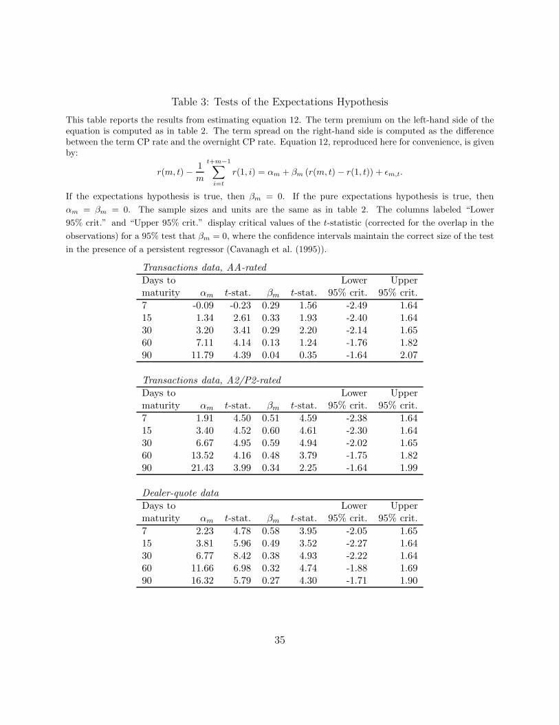
Table 3: Tests of the Expectations Hypothesis

This table reports the results from estimating equation 12. The term premium on the left-hand side of theequation is computed as in table 2. The term spread on the right-hand side is computed as the differencebetween the term CP rate and the overnight CP rate. Equation 12, reproduced here for convenience, is givenby:

r(m, t) − 1m

t+m−1∑i=t

r(1, i) = αm + βm (r(m, t) − r(1, t)) + εm,t.

If the expectations hypothesis is true, then βm = 0. If the pure expectations hypothesis is true, thenαm = βm = 0. The sample sizes and units are the same as in table 2. The columns labeled “Lower95% crit.” and “Upper 95% crit.” display critical values of the t-statistic (corrected for the overlap in theobservations) for a 95% test that βm = 0, where the confidence intervals maintain the correct size of the testin the presence of a persistent regressor (Cavanagh et al. (1995)).

Transactions data, AA-ratedDays to Lower Uppermaturity αm t-stat. βm t-stat. 95% crit. 95% crit.7 -0.09 -0.23 0.29 1.56 -2.49 1.6415 1.34 2.61 0.33 1.93 -2.40 1.6430 3.20 3.41 0.29 2.20 -2.14 1.6560 7.11 4.14 0.13 1.24 -1.76 1.8290 11.79 4.39 0.04 0.35 -1.64 2.07

Transactions data, A2/P2-ratedDays to Lower Uppermaturity αm t-stat. βm t-stat. 95% crit. 95% crit.7 1.91 4.50 0.51 4.59 -2.38 1.6415 3.40 4.52 0.60 4.61 -2.30 1.6430 6.67 4.95 0.59 4.94 -2.02 1.6560 13.52 4.16 0.48 3.79 -1.75 1.8290 21.43 3.99 0.34 2.25 -1.64 1.99

Dealer-quote dataDays to Lower Uppermaturity αm t-stat. βm t-stat. 95% crit. 95% crit.7 2.23 4.78 0.58 3.95 -2.05 1.6515 3.81 5.96 0.49 3.52 -2.27 1.6430 6.77 8.42 0.38 4.93 -2.22 1.6460 11.66 6.98 0.32 4.74 -1.88 1.6990 16.32 5.79 0.27 4.30 -1.71 1.90

35

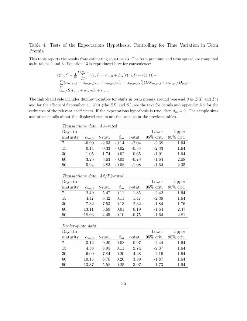
Table 4: Tests of the Expectations Hypothesis, Controlling for Time Variation in TermPremia

This table reports the results from estimating equation 13. The term premium and term spread are computedas in tables 2 and 3. Equation 13 is reproduced here for convenience:

r(m, t) − 1m

t+m−1∑i=t

r(1, i) = αm,0 + βm(r(m, t) − r(1, t))+∑yr

(αm,yr,1 + αm,yr,2τm + αm,yr,3τ2m + αm,yr,4τ

3m)DXm,yr,t + αm,yr,5Dyr,t+

αm,6SXm,t + αm,7St + εm,t,

The right-hand side includes dummy variables for shifts in term premia around year-end (the DX· and D·)and for the effects of September 11, 2001 (the SX· and S·); see the text for details and appendix A.2 for theestimates of the relevant coefficients. If the expectations hypothesis is true, then βm = 0. The sample sizesand other details about the displayed results are the same as in the previous tables.

Transactions data, AA-ratedDays to Lower Uppermaturity αm,0 t-stat. βm t-stat. 95% crit. 95% crit.7 -0.90 -2.63 -0.14 -2.04 -2.38 1.6415 0.14 0.33 -0.02 -0.35 -2.33 1.6430 1.05 1.74 0.02 0.65 -1.91 1.6460 3.26 3.63 -0.03 -0.73 -1.64 2.0890 5.94 3.83 -0.08 -1.08 -1.64 2.35

Transactions data, A2/P2-ratedDays to Lower Uppermaturity αm,0 t-stat. βm t-stat. 95% crit. 95% crit.7 2.49 5.47 0.11 1.35 -2.42 1.6415 4.47 6.42 0.11 1.47 -2.38 1.6430 7.32 7.53 0.13 2.32 -1.84 1.7660 13.11 5.69 0.01 0.19 -1.64 2.4790 18.96 4.45 -0.10 -0.75 -1.64 2.81

Dealer-quote dataDays to Lower Uppermaturity αm,0 t-stat. βm t-stat. 95% crit. 95% crit.7 3.12 9.20 0.08 0.97 -2.44 1.6415 4.38 8.95 0.11 2.74 -2.37 1.6430 6.09 7.84 0.20 4.28 -2.16 1.6460 10.13 6.70 0.20 3.89 -1.87 1.6490 13.37 5.58 0.25 3.97 -1.73 1.94

36

Table 5: Goodness-of-Fit Measures

The table compares the adjusted-R2 goodness-of-fit measure for the regressions in tables 3 and 4 above.The columns labeled “No Yr-end” show the goodness-of-fit measures for the regressions in table 3, while thecolumns labeled “Yr-end” show the goodness-of-fit measures for the corresponding regressions in table 4.The adjusted-R2 figures are in percent.

Transactions dataAA-rated A2/P2-rated Dealer-quote data

Days to No No Nomaturity Yr-end Yr-end Yr-end Yr-end Yr-end Yr-end7 7 45 26 48 34 6315 16 60 43 72 31 6530 16 66 45 78 20 5460 4 61 28 73 15 5290 0 60 14 67 11 49

37

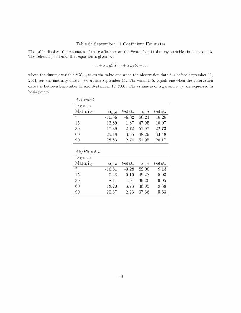
Table 6: September 11 Coefficient Estimates

The table displays the estimates of the coefficients on the September 11 dummy variables in equation 13.The relevant portion of that equation is given by:

. . . + αm,6SXm,t + αm,7St + . . .

where the dummy variable SXm,t takes the value one when the observation date t is before September 11,2001, but the maturity date t + m crosses September 11. The variable St equals one when the observationdate t is between September 11 and September 18, 2001. The estimates of αm,6 and αm,7 are expressed inbasis points.

AA-ratedDays toMaturity αm,6 t-stat. αm,7 t-stat.7 -10.36 -6.82 86.21 18.2815 12.89 1.87 47.95 10.0730 17.89 2.72 51.97 22.7360 25.18 3.55 48.29 33.4890 28.83 2.74 51.95 20.17

A2/P2-ratedDays toMaturity αm,6 t-stat. αm,7 t-stat.7 -16.81 -3.28 82.98 9.1315 0.48 0.10 49.28 5.9330 8.11 1.94 39.20 9.9560 18.20 3.73 36.05 9.3890 20.37 2.23 37.36 5.63

38

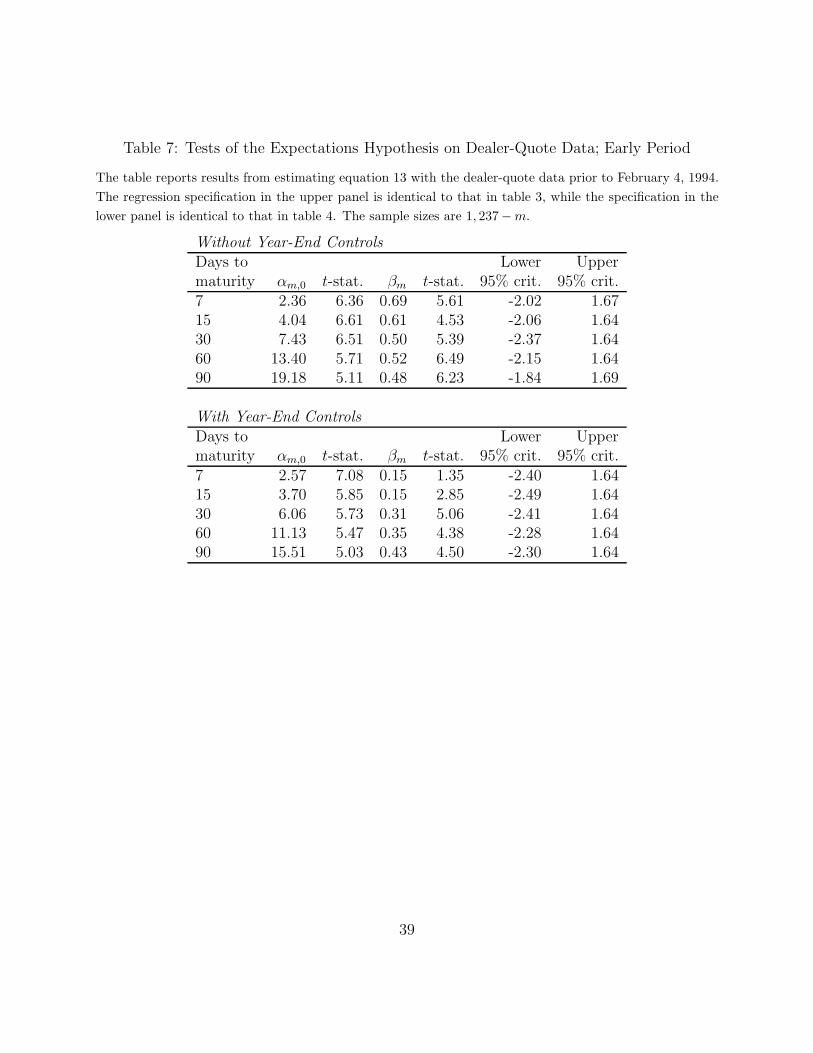
Table 7: Tests of the Expectations Hypothesis on Dealer-Quote Data; Early Period

The table reports results from estimating equation 13 with the dealer-quote data prior to February 4, 1994.The regression specification in the upper panel is identical to that in table 3, while the specification in thelower panel is identical to that in table 4. The sample sizes are 1, 237− m.

Without Year-End ControlsDays to Lower Uppermaturity αm,0 t-stat. βm t-stat. 95% crit. 95% crit.7 2.36 6.36 0.69 5.61 -2.02 1.6715 4.04 6.61 0.61 4.53 -2.06 1.6430 7.43 6.51 0.50 5.39 -2.37 1.6460 13.40 5.71 0.52 6.49 -2.15 1.6490 19.18 5.11 0.48 6.23 -1.84 1.69

With Year-End ControlsDays to Lower Uppermaturity αm,0 t-stat. βm t-stat. 95% crit. 95% crit.7 2.57 7.08 0.15 1.35 -2.40 1.6415 3.70 5.85 0.15 2.85 -2.49 1.6430 6.06 5.73 0.31 5.06 -2.41 1.6460 11.13 5.47 0.35 4.38 -2.28 1.6490 15.51 5.03 0.43 4.50 -2.30 1.64

39

Table 8: Tests of the Expectations Hypothesis on Dealer-Quote Data; Late Period

The table reports results from estimating equation 13 with the dealer-quote data starting from February 4,1994. The regression specification in the upper panel is identical to that in table 3, while the specificationin the lower panel is identical to that in table 4. The sample sizes are 832 − m.

Without Year-End ControlsDays to Lower Uppermaturity αm,0 t-stat. βm t-stat. 95% crit. 95% crit.7 4.11 7.36 0.12 1.27 -2.45 1.6415 5.83 7.67 0.15 1.75 -2.39 1.6430 7.05 5.80 0.21 2.18 -2.17 1.6460 9.54 6.84 0.19 2.34 -2.11 1.6490 10.39 6.85 0.23 3.64 -1.87 1.71

With Year-End ControlsDays to Lower Uppermaturity αm,0 t-stat. βm t-stat. 95% crit. 95% crit.7 4.73 9.15 -0.10 -1.66 -2.49 1.6415 6.13 8.49 0.00 0.06 -2.32 1.6430 7.40 7.27 0.06 1.02 -2.24 1.6460 9.31 6.93 0.11 2.61 -2.10 1.6490 9.35 4.38 0.21 4.17 -1.74 1.84

40

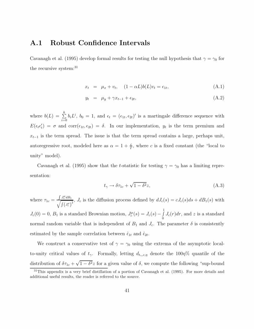
A.1 Robust Confidence Intervals

Cavanagh et al. (1995) develop formal results for testing the null hypothesis that γ = γ0 for

the recursive system:31

xt = µx + vt, (1 − αL)b(L)vt = ε1t, (A.1)

yt = µy + γxt−1 + ε2t, (A.2)

where b(L) =k∑

i=0biL

i, b0 = 1, and εt = (ε1t, ε2t)′ is a martingale difference sequence with

E(εtε′t) = σ and corr(ε1t, ε2t) = δ. In our implementation, yt is the term premium and

xt−1 is the term spread. The issue is that the term spread contains a large, perhaps unit,

autoregressive root, modeled here as α = 1 + cT, where c is a fixed constant (the “local to

unity” model).

Cavanagh et al. (1995) show that the t-statistic for testing γ = γ0 has a limiting repre-

sentation:

tγ → δτ1c +√

1 − δ2z, (A.3)

where τ1c =∫

Jµc dB1√∫(Jµ

c )2, Jc is the diffusion process defined by dJc(s) = cJc(s)ds + dB1(s) with

Jc(0) = 0, B1 is a standard Brownian motion, Jµc (s) = Jc(s)−

1∫0

Jc(r)dr, and z is a standard

normal random variable that is independent of B1 and Jc. The parameter δ is consistently

estimated by the sample correlation between ε̂1t and ε̂2t.

We construct a conservative test of γ = γ0 using the extrema of the asymptotic local-

to-unity critical values of tγ. Formally, letting dtγ ,c,η denote the 100η% quantile of the

distribution of δτ1c +√

1 − δ2z for a given value of δ, we compute the following “sup-bound

31This appendix is a very brief distillation of a portion of Cavanagh et al. (1995). For more details andadditional useful results, the reader is referred to the source.

41

confidence interval” by Monte Carlo simulation:

(dη, d̄η) =(infc

dtγ ,c,η, supc

dtγ ,c,η

). (A.4)

Intuitively, the procedure amounts to picking the most conservative confidence limits across

a sequence of values of c.

The following Matlab code details our implementation of the Cavanagh et al. (1995)

procedure for calculating the conservative sup-bound confidence intervals:32

function [tstat, crit] = supbound_dum(x, y, d, p);%%%%%%%%%%%%%%%%%%%%%%%%%%%%%%%%%%%%%%%%%%%%%%%%%%%%%%%%%%%%%%%%%%%%% Computes sup-bound critical values in a regression of %% y(t) on d(t) and x(t-1,1); the routine will also add a constant. %% Autocorrelation robust standard errors are used with truncation %% p. d(t) is a set of calendar dummy variables with number of %% rows equal to the number of rows of y and x and any number of %% columns (subject to computational limits.) %% It is assumed that the number of observations is large enough %% that the number of rows of d can serve as the number of Monte %% Carlo iterations in the calculation of the supbounds. %% NOTE: Before calling this routine, set the seed for Matlab’s %% random number generator if you want results that can be %% replicated exactly. %%%%%%%%%%%%%%%%%%%%%%%%%%%%%%%%%%%%%%%%%%%%%%%%%%%%%%%%%%%%%%%%%%%%%t=size(x,1);q=y(1:t-1);w=[ones(t-1,1) d(1:t-1,:) x(1:t-1)];k=size(w,2);bhat=inv(w’*w)*w’*q;u=q-w*bhat;z=kron(u,ones(1,k)).*w;for j=1:p+1;lb(:,:,j)=((p+2-j)/(p+1))*z(j:t-1,:)’*z(1:t-j,:);

end; %NWsigma=sum(lb,3)+(sum(lb,3)’)-lb(:,:,1);clear lb;a=inv(w’*w)*sigma*inv(w’*w);

32This program incorporates minor modifications to a program kindly provided to the authors by JonathanWright. We modified Wright’s program to allow for calendar dummy variables in the regression specification.

42

w=[ones(t-1,1) d(2:t,:) x(1:t-1)];q=x(2:t,:);v=q-(w*inv(w’*w)*w’*q);z=[u v];for j=1:p+1;lb(:,:,j)=((p+2-j)/(p+1))*z(j:t-1,:)’*z(1:t-j,:);

end; %NWsigma=sum(lb,3)+(sum(lb,3)’)-lb(:,:,1);delta=sigma(1,2)/sqrt(sigma(1,1)*sigma(2,2));tstat=bhat(k)/sqrt(a(k,k));s=size(d,1);dum=[ones(s,1) d];dp=dum*inv(dum’*dum)*dum’;b1=zeros(s,1000);sa=zeros(1000,1);stat=zeros(1000,1);sb1=zeros(3,31);sb2=zeros(3,31);u=randn(s,31000)./sqrt(s);eps=randn(1000,31);for k=1:31;alpha=1+((1-k)/1000);b1=filter(1,[1;-alpha],u(1:s,(k-1)*1000+1:k*1000));b1=b1-dp*b1;sa=sum(b1(1:s-1,1:1000).*u(2:s,(k-1)*1000+1:k*1000))./sqrt(mean((b1.^2)));stat=(delta.*sa’)+(sqrt(1-(delta^2)).*eps(1:1000,k));stat=sort(stat);sb1(1:3,k)=stat([10;50;100]);sb2(1:3,k)=stat([990;950;900]);

end;sb1(1:3,32)=norminv([0.01 0.05 0.10]’);sb2(1:3,32)=norminv([0.99 0.95 0.90]’);crit=[[0.01 0.05 0.10]’ min(sb1’)’ max(sb2’)’];

43

A.2 Dummy Variable Coefficient Estimates

The tables in this appendix display the estimated coefficients on the dummy variables in

equation 13 that control for year-end and September 11 effects. Tables A.1-A.3 report the

results from the transactions data for AA-rated firms, the transaction data for A2/P2-rated

firms, and the dealer-quote data, respectively. Tables A.4 and A.5 show the estimates for

the sample splits on the dealer-quote data. Below each coefficient estimate we report its

t-statistic, where the underlying standard errors are adjusted for the overlap in the observa-

tions.

44

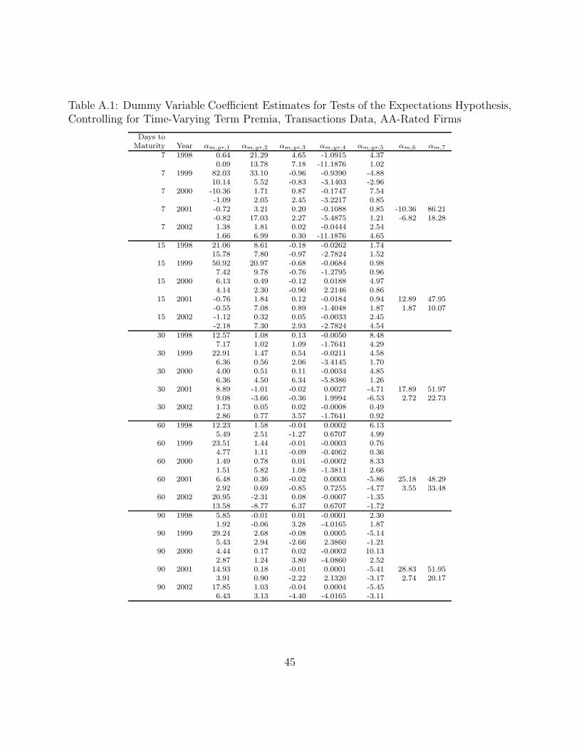
Table A.1: Dummy Variable Coefficient Estimates for Tests of the Expectations Hypothesis,Controlling for Time-Varying Term Premia, Transactions Data, AA-Rated Firms

Days toMaturity Year αm,yr,1 αm,yr,2 αm,yr,3 αm,yr,4 αm,yr,5 αm,6 αm,7

7 1998 0.64 21.29 4.65 -1.0915 4.370.09 13.78 7.18 -11.1876 1.02

7 1999 82.03 33.10 -0.96 -0.9390 -4.8810.14 5.52 -0.83 -3.1403 -2.96

7 2000 -10.36 1.71 0.87 -0.1747 7.54-1.09 2.05 2.45 -3.2217 0.85

7 2001 -0.72 3.21 0.20 -0.1088 0.85 -10.36 86.21-0.82 17.03 2.27 -5.4875 1.21 -6.82 18.28

7 2002 1.38 1.81 0.02 -0.0444 2.541.66 6.99 0.30 -11.1876 4.65

15 1998 21.06 8.61 -0.18 -0.0262 1.7415.78 7.80 -0.97 -2.7824 1.52

15 1999 50.92 20.97 -0.68 -0.0684 0.987.42 9.78 -0.76 -1.2795 0.96

15 2000 6.13 0.49 -0.12 0.0188 4.974.14 2.30 -0.90 2.2146 0.86

15 2001 -0.76 1.84 0.12 -0.0184 0.94 12.89 47.95-0.55 7.08 0.89 -1.4048 1.87 1.87 10.07

15 2002 -1.12 0.32 0.05 -0.0033 2.45-2.18 7.30 2.93 -2.7824 4.54

30 1998 12.57 1.08 0.13 -0.0050 8.487.17 1.02 1.09 -1.7641 4.29

30 1999 22.91 1.47 0.54 -0.0211 4.586.36 0.56 2.06 -3.4145 1.70

30 2000 4.00 0.51 0.11 -0.0034 4.856.36 4.50 6.34 -5.8386 1.26

30 2001 8.89 -1.01 -0.02 0.0027 -4.71 17.89 51.979.08 -3.66 -0.36 1.9994 -6.53 2.72 22.73

30 2002 1.73 0.05 0.02 -0.0008 0.492.86 0.77 3.57 -1.7641 0.92

60 1998 12.23 1.58 -0.04 0.0002 6.135.49 2.51 -1.27 0.6707 4.99

60 1999 23.51 1.44 -0.01 -0.0003 0.764.77 1.11 -0.09 -0.4062 0.36

60 2000 1.49 0.78 0.01 -0.0002 8.331.51 5.82 1.08 -1.3811 2.66

60 2001 6.48 0.36 -0.02 0.0003 -5.86 25.18 48.292.92 0.69 -0.85 0.7255 -4.77 3.55 33.48

60 2002 20.95 -2.31 0.08 -0.0007 -1.3513.58 -8.77 6.37 0.6707 -1.72

90 1998 5.85 -0.01 0.01 -0.0001 2.301.92 -0.06 3.28 -4.0165 1.87

90 1999 29.24 2.68 -0.08 0.0005 -5.145.43 2.94 -2.66 2.3860 -1.21

90 2000 4.44 0.17 0.02 -0.0002 10.132.87 1.24 3.80 -4.0860 2.52

90 2001 14.93 0.18 -0.01 0.0001 -5.41 28.83 51.953.91 0.90 -2.22 2.1320 -3.17 2.74 20.17

90 2002 17.85 1.03 -0.04 0.0004 -5.456.43 3.13 -4.40 -4.0165 -3.11

45

Table A.2: Dummy Variable Coefficient Estimates for Tests of the Expectations Hypothesis,Controlling for Time-Varying Term Premia,Transactions Data, A2/P2-Rated Firms

Days toMaturity Year αm,yr,1 αm,yr,2 αm,yr,3 αm,yr,4 αm,yr,5 αm,6 αm,7

7 1998 4.84 23.99 4.57 -1.1071 1.860.51 9.19 5.34 -7.7745 0.30

7 1999 53.70 24.41 0.04 -0.7402 -0.669.58 6.67 0.08 -4.7307 -0.39

7 2000 24.21 17.70 0.81 -0.5492 5.721.81 8.39 1.43 -4.1092 0.47

7 2001 5.58 0.36 1.67 0.7253 3.63 -16.81 82.982.08 0.50 37.93 10.2709 1.31 -3.28 9.13

7 2002 12.19 0.08 -0.57 0.1053 -0.856.98 0.34 -6.64 -7.7745 -0.71

15 1998 24.51 5.76 1.62 -0.1289 -1.124.95 1.32 1.56 -2.3771 -0.33

15 1999 44.17 20.47 0.40 -0.1349 -1.1310.55 12.34 1.17 -6.1224 -0.90

15 2000 11.07 10.36 1.11 -0.1039 -16.364.98 12.76 4.63 -6.1429 -1.59

15 2001 8.92 5.69 -0.06 -0.0258 12.81 0.48 49.285.98 8.60 -0.42 -1.4789 5.03 0.10 5.93

15 2002 -4.17 3.25 0.07 -0.0152 -1.34-4.33 11.88 1.73 -2.3771 -1.59

30 1998 46.17 3.95 -0.17 0.0013 10.9815.40 3.55 -1.61 0.5043 6.70

30 1999 33.66 4.12 0.27 -0.0141 11.247.07 1.13 0.75 -1.6416 2.47

30 2000 -0.53 5.18 0.12 -0.0065 -28.58-0.43 15.40 2.59 -4.7210 -4.84

30 2001 21.34 3.63 -0.32 0.0080 2.69 8.11 39.2014.33 6.06 -4.24 3.5781 1.86 1.94 9.95

30 2002 10.47 0.75 0.01 -0.0009 6.125.86 1.06 0.10 0.5043 4.97

60 1998 45.58 4.41 -0.13 0.0010 8.4619.75 6.01 -4.28 2.6102 4.75

60 1999 31.21 3.08 -0.06 0.0002 4.655.64 2.33 -0.93 0.2066 1.84

60 2000 -12.85 1.92 -0.04 0.0010 -24.00-6.57 5.40 -2.47 3.9108 -5.64

60 2001 33.55 1.79 -0.07 0.0006 -8.97 18.20 36.0519.27 4.96 -3.73 2.6894 -4.65 3.73 9.38

60 2002 43.89 -3.17 0.12 -0.0011 -1.1719.66 -9.98 8.44 2.6102 -0.63

90 1998 -8.82 3.08 -0.02 -0.0001 13.77-1.19 5.51 -1.35 -0.7041 3.22

90 1999 37.83 3.41 -0.08 0.0005 -3.365.88 2.77 -2.07 1.6526 -0.54

90 2000 -11.78 0.63 -0.01 0.0002 -15.33-3.69 2.24 -1.06 2.9103 -2.85

90 2001 10.60 2.83 -0.05 0.0002 -12.15 20.37 37.361.57 5.97 -4.89 2.8729 -3.59 2.23 5.63

90 2002 21.58 1.34 -0.03 0.0002 6.215.74 4.33 -3.39 -0.7041 2.73

46

Table A.3: Dummy Variable Coefficient Estimates for Tests of theExpectations Hypothesis, Controlling for Time-Varying Term Pre-mia, Dealer-Quote Data

Days toMaturity Year αm,yr,1 αm,yr,2 αm,yr,3 αm,yr,4 αm,yr,5

7 1989 -35.82 10.66 4.45 -0.4876 3.27-5.74 3.06 10.08 -1.1031 1.71

7 1990 -20.99 61.01 9.03 -2.0625 9.15-1.44 11.69 7.85 -9.6117 1.62

7 1991 -7.07 49.01 4.78 -1.5415 2.99-1.67 10.43 11.22 -9.5760 1.09

7 1992 -26.53 6.94 2.73 -0.5276 16.93-16.47 6.93 18.15 -13.9015 15.81

7 1993 -8.65 4.61 0.82 -0.1586 6.19-4.99 6.99 8.28 -7.1808 4.17

7 1994 -7.03 7.18 0.48 -0.2235 10.44-5.68 5.58 3.61 -3.8704 11.31

7 1995 9.98 6.02 -0.27 -0.2164 3.444.69 5.00 -5.93 -4.4006 4.34

7 1996 -7.26 7.25 1.78 -0.1833 8.31-2.68 2.51 4.97 -1.5691 3.58

15 1989 2.98 -0.28 -0.23 0.0420 1.591.45 -0.74 -1.19 0.2203 1.23

15 1990 16.06 14.58 0.91 -0.0923 22.982.83 11.70 2.59 -4.0051 10.04

15 1991 -7.77 5.13 1.25 -0.0833 3.06-2.79 7.85 6.33 -6.3428 1.16

15 1992 12.41 6.95 -1.34 0.0577 12.215.08 3.89 -3.18 2.6861 5.37

15 1993 1.56 2.07 -0.25 0.0121 5.441.45 7.94 -3.29 2.9951 4.52

15 1994 3.81 2.56 -0.18 0.0043 13.701.71 5.77 -1.00 0.3634 6.09

15 1995 7.99 1.22 -0.42 0.0295 3.254.96 5.90 -3.51 3.3557 3.45

15 1996 6.01 2.99 -0.15 0.0146 8.042.58 7.85 -0.90 1.3917 6.43

30 1989 -13.51 0.86 -0.01 0.0017 -3.30-9.58 2.26 -0.19 0.0290 -2.53

30 1990 23.19 -2.28 0.18 0.0004 32.256.26 -1.31 0.84 0.0649 18.75

30 1991 25.32 0.23 -0.07 0.0036 2.8516.83 0.29 -0.75 1.6264 1.14

30 1992 25.85 5.07 -0.49 0.0101 13.1410.65 7.78 -8.12 7.4137 9.72

30 1993 9.33 2.57 -0.26 0.0059 3.04(Continued next page...)

47

Table A.3: (continued)

Days toMaturity Year αm,yr,1 αm,yr,2 αm,yr,3 αm,yr,4 αm,yr,5

7.19 4.63 -5.08 5.3451 2.6230 1994 18.33 4.04 -0.34 0.0072 13.28

11.82 7.03 -7.32 7.5515 8.3830 1995 -3.48 0.53 0.02 -0.0010 4.18

-4.20 3.05 0.78 -1.2961 5.0030 1996 1.02 -0.10 0.03 0.0009 3.96

0.82 -0.31 0.85 0.8156 2.8060 1989 1.27 -0.91 0.01 0.0002 -6.22

0.75 -5.98 1.82 0.0231 -3.8760 1990 7.56 3.29 -0.10 0.0011 46.31

2.66 3.94 -2.32 2.0314 16.5460 1991 23.05 0.71 -0.02 0.0002 -6.94

9.85 0.99 -0.50 0.4289 -2.5060 1992 4.56 2.39 -0.05 0.0001 8.74

2.66 7.59 -3.39 0.6062 5.6060 1993 2.42 2.07 -0.08 0.0007 -9.23

1.59 11.85 -9.62 7.5475 -5.3160 1994 -18.72 1.31 0.03 -0.0008 13.06

-4.80 3.97 2.06 -4.4086 6.6060 1995 -6.27 -0.01 0.02 -0.0002 10.85

-4.13 -0.05 3.16 -3.1137 6.7160 1996 -9.35 0.33 -0.02 0.0004 4.24

-6.09 1.42 -1.18 2.1919 2.7990 1989 15.42 -0.91 0.01 0.0001 -8.30

3.95 -1.93 0.34 0.0048 -2.7890 1990 14.00 0.31 0.02 -0.0002 55.88

4.41 1.03 1.74 -2.0219 19.7190 1991 32.12 1.10 -0.03 0.0002 -9.22

11.13 3.28 -2.78 2.1752 -2.8590 1992 -5.10 -0.28 0.04 -0.0004 9.50

-1.47 -1.24 7.27 -8.7713 4.6190 1993 -1.32 0.43 -0.01 0.0000 -13.63

-0.50 1.45 -0.83 0.4195 -4.7290 1994 -5.33 -1.47 0.06 -0.0004 13.15

-1.15 -3.46 4.30 -4.1200 3.8990 1995 -3.83 -0.52 0.02 -0.0002 5.27

-1.43 -3.45 4.53 -4.2905 2.2590 1996 -4.42 -0.17 -0.00 0.0001 -0.93

-1.43 -0.59 -0.27 1.2788 -0.42

48

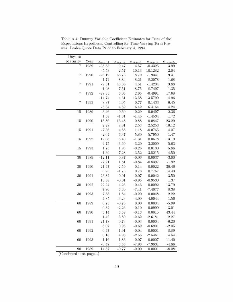
Table A.4: Dummy Variable Coefficient Estimates for Tests of theExpectations Hypothesis, Controlling for Time-Varying Term Pre-mia, Dealer-Quote Data Prior to February 4, 1994

Days toMaturity Year αm,yr,1 αm,yr,2 αm,yr,3 αm,yr,4 αm,yr,5

7 1989 -38.83 9.47 4.57 -0.4325 3.99-5.53 2.57 10.13 10.1282 2.04

7 1990 -26.19 56.73 8.79 -1.9341 9.41-1.74 8.84 8.21 8.2078 1.68

7 1991 -9.31 45.36 4.51 -1.4234 3.88-1.93 7.51 8.75 8.7497 1.35

7 1992 -27.35 6.05 2.65 -0.4991 17.68-14.74 4.51 13.58 13.5799 14.96

7 1993 -8.87 4.05 0.77 -0.1433 6.45-5.34 4.59 6.42 6.4164 4.24

15 1989 3.46 -0.60 -0.29 0.0497 2.361.58 -1.31 -1.45 -1.4534 1.72

15 1990 13.86 13.48 0.88 -0.0847 23.292.28 8.91 2.53 2.5253 10.12

15 1991 -7.36 4.68 1.18 -0.0765 4.07-2.64 6.37 5.80 5.7950 1.47

15 1992 12.08 6.40 -1.31 0.0578 13.194.75 3.60 -3.20 -3.2009 5.63

15 1993 1.75 1.95 -0.26 0.0130 5.861.39 7.28 -3.52 -3.5215 4.50

30 1989 -12.11 0.87 -0.06 0.0037 -3.00-7.21 1.81 -0.84 -0.8397 -1.92

30 1990 21.47 -2.59 0.14 0.0022 30.466.25 -1.75 0.78 0.7767 14.43

30 1991 23.82 -0.01 -0.07 0.0042 3.5013.38 -0.01 -0.95 -0.9530 1.37

30 1992 22.24 4.26 -0.43 0.0092 13.797.80 6.30 -7.41 -7.4077 8.38

30 1993 7.88 1.84 -0.20 0.0048 2.224.85 3.23 -4.00 -4.0044 1.56

60 1989 0.73 -0.76 0.00 0.0004 -5.990.32 -2.26 0.10 0.0999 -3.01

60 1990 5.14 3.58 -0.13 0.0015 43.441.42 3.80 -2.62 -2.6181 12.27

60 1991 21.78 0.73 -0.03 0.0004 -6.208.07 0.95 -0.69 -0.6901 -2.05

60 1992 0.47 1.91 -0.04 0.0001 8.890.18 4.98 -2.55 -2.5461 4.54

60 1993 -1.16 1.83 -0.07 0.0007 -11.40-0.47 8.55 -7.98 -7.9831 -4.86

90 1989 14.87 -0.77 -0.00 0.0001 -8.08(Continued next page...)

49

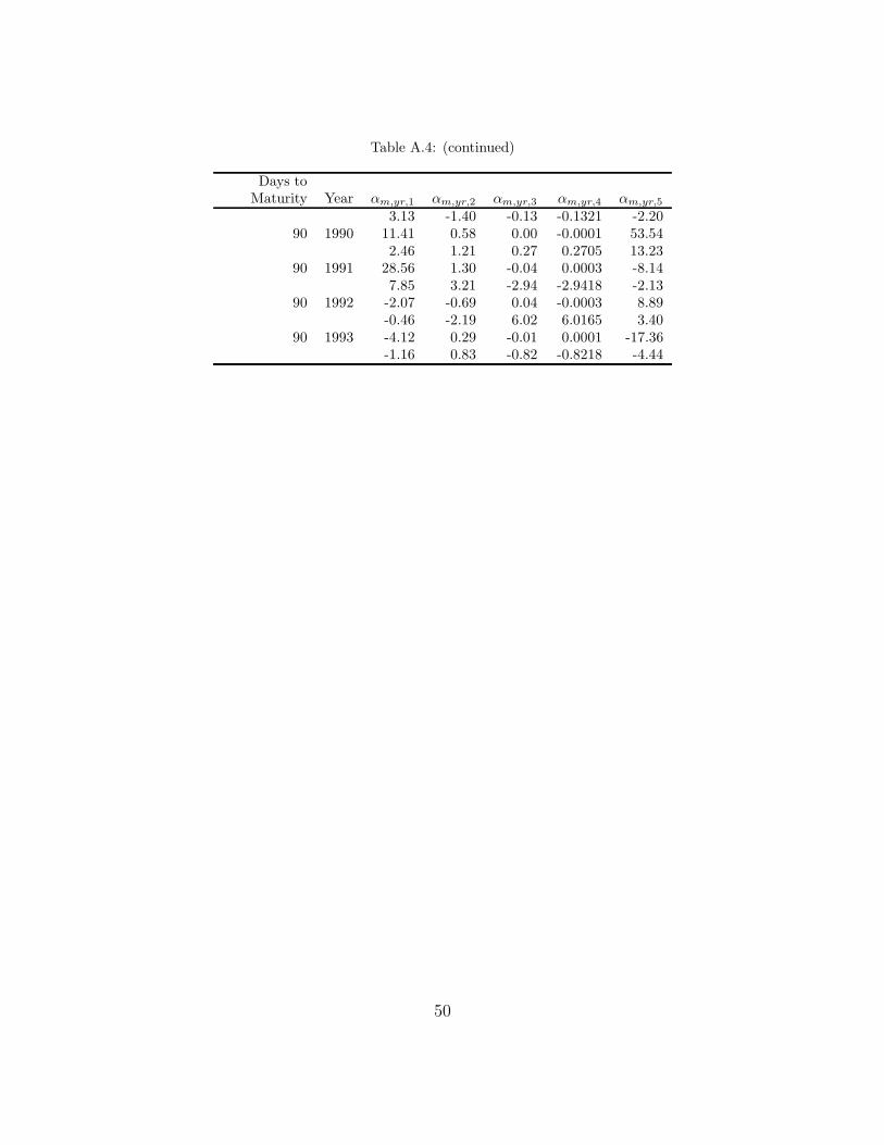
Table A.4: (continued)

Days toMaturity Year αm,yr,1 αm,yr,2 αm,yr,3 αm,yr,4 αm,yr,5

3.13 -1.40 -0.13 -0.1321 -2.2090 1990 11.41 0.58 0.00 -0.0001 53.54

2.46 1.21 0.27 0.2705 13.2390 1991 28.56 1.30 -0.04 0.0003 -8.14

7.85 3.21 -2.94 -2.9418 -2.1390 1992 -2.07 -0.69 0.04 -0.0003 8.89

-0.46 -2.19 6.02 6.0165 3.4090 1993 -4.12 0.29 -0.01 0.0001 -17.36

-1.16 0.83 -0.82 -0.8218 -4.44

50

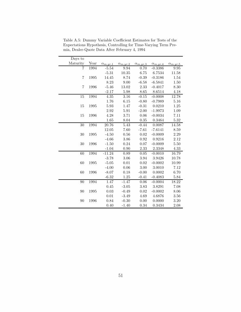
Table A.5: Dummy Variable Coefficient Estimates for Tests of theExpectations Hypothesis, Controlling for Time-Varying Term Pre-mia, Dealer-Quote Data After February 4, 1994

Days toMaturity Year αm,yr,1 αm,yr,2 αm,yr,3 αm,yr,4 αm,yr,5

7 1994 -5.54 9.94 0.70 -0.3386 9.95-5.31 10.35 6.75 6.7534 11.58

7 1995 14.45 8.74 -0.39 -0.3186 1.548.23 9.00 -6.58 -6.5841 1.50

7 1996 -5.46 13.02 2.33 -0.4017 8.30-2.17 5.98 8.65 8.6514 4.18

15 1994 4.35 3.16 -0.15 -0.0008 12.781.76 6.15 -0.80 -0.7989 5.16

15 1995 5.93 1.47 -0.31 0.0210 1.252.92 5.91 -2.00 -1.9973 1.09

15 1996 4.28 3.71 0.06 -0.0034 7.111.65 8.04 0.35 0.3464 5.32

30 1994 20.76 5.43 -0.44 0.0087 14.5812.05 7.60 -7.61 -7.6141 8.59

30 1995 -4.50 0.56 0.02 -0.0009 2.29-4.66 3.86 0.92 0.9216 2.12

30 1996 -1.50 0.24 0.07 -0.0009 5.50-1.04 0.90 2.33 2.3348 4.33

60 1994 -11.24 0.89 0.05 -0.0010 16.79-3.78 3.06 3.94 3.9426 10.78

60 1995 -5.05 0.01 0.02 -0.0002 10.99-4.00 0.06 3.00 3.0010 7.12

60 1996 -8.07 0.18 -0.00 0.0002 6.70-6.32 1.25 -0.41 -0.4083 5.84

90 1994 1.47 -1.47 0.06 -0.0004 18.220.45 -3.05 3.83 3.8291 7.08

90 1995 0.03 -0.49 0.02 -0.0002 8.060.01 -3.49 4.69 4.6876 3.56

90 1996 0.84 -0.30 0.00 0.0000 3.200.40 -1.40 0.34 0.3434 2.08

51

References

Balduzzi, P., Bertola, G. and Foresi, S.: 1997, A model of target changes and the termstructure of interest rates, Journal of Monetary Economics 39, 223–249.

Bekaert, G., Hodrick, R. J. and Marshall, D.: 2001, Peso problem explanations for termstructure anomalies, Journal of Monetary Economics 48(2), 241–270.

Bekaert, G., Hodrick, R. J. and Marshall, D. A.: 1997, On biases in tests of the expecta-tions hypothesis of the term structure of interest rates, Journal of Financial Economics44, 309–348.

Campbell, J. Y., Lo, A. W. and MacKinlay, A. C.: 1996, The Econometrics of FinancialMarkets, Princeton University Press, Princeton, N.J.

Cavanagh, C. L., Elliott, G. and Stock, J. H.: 1995, Inference in models with nearly inte-grated regressors, Econometric Theory 11, 1131–1147.

Cook, T. and Hahn, T.: 1990, Interest rate expectations and the slope of the money marketyield curve, Federal Reserve Bank of Richmond Economic Review 76(5), 3–26.

Cook, T. and Lawler, T.: 1983, The behavior of the spread between Treasury bill rates andprivate money market rates since 1978. Federal Reserve Bank of Richmond WorkingPaper 83-4.

Dahlquist, M. and Jonsson, G.: 1995, The information in Swedish short-maturity forwardrates, European Economic Review 39, 1115–1131.

Duffee, G. R.: 1996, Idiosyncratic variation of Treasury bill yields, Journal of Finance51(2), 527–551.

Fama, E. F.: 1986, Term premiums and default premiums in money markets, Journal ofFinancial Economics 17, 175–196.

Gerlach, S. and Smets, F.: 1997, The term structure of euro-rates: Some evidence in supportof the expectations hypothesis, Journal of International Money and Finance 16(2), 305–321.

Hardouvelis, G. A.: 1994, The term structure spread and future changes in long and shortrates in G7 countries: Is there a puzzle?, Journal of Monetary Economics 33, 255–283.

Kozicki, S. and Tinsley, P. A.: 2001, Shifting endpoints in the term structure of interestrates, Journal of Monetary Economics 47, 613–652.

52

Lange, J., Sack, B. and Whitesell, W.: 2003, Anticipations of monetary policy in financialmarkets, Journal of Money, Credit, and Banking 35, 889–909.

Longstaff, F. A.: 2000, The term structure of very short-term rates: New evidence for theexpectations hypothesis, Journal of Financial Economics 58(3), 397–415.

Mankiw, N. G. and Miron, J. A.: 1986, The changing behavior of the term structure ofinterest rates, Quarterly Journal of Economics 101(2), 211–228.

Melino, A.: 1988, The term structure of interest rates: Evidence and theory, Journal ofEconomic Surveys 2(4), 335–366.

Musto, D. K.: 1997, Portfolio disclosures and year-end price shifts, The Journal of Finance52(4), 1563–1588.

Musto, D. K.: 1999, Investment decisions depend on portfolio disclosures, The Journal ofFinance 54(3), 935–952.

Roberds, W., Runkle, D. and Whiteman, C. H.: 1996, A daily view of yield spreads andshort-term interest rate movements, Journal of Money, Credit and Banking 28(1), 34–53.

Roush, J. E.: 2001, Evidence uncovered: Long-term interest rates, monetary policy, and theexpectations theory. Board of Governors of the Federal Reserve System, InternationalFinance Discussion Paper No. 712.

Rudebusch, G. D.: 1995, Federal Reserve interest rate targeting, rational expectations, andthe term structure, Journal of Monetary Economics 35, 245–274.

Shiller, R. J.: 1990, The term structure of interest rates, in B. Friedman and F. Hahn (eds),Handbook of Monetary Economics, North-Holland, Amsterdam.

Simon, D. P.: 1990, Expectations and the Treasury bill-federal funds rate spread over recentmonetary policy regimes, Journal of Finance 45, 567–577.

Stigum, M. L.: 1990, The Money Market, 3 edn, McGraw-Hill, New York.

Swanson, E. T.: 2004, Federal Reserve transparency and financial market forecasts of short-term interest rates. Board of Governors of the Federal Reserve System, Finance andEconomics Discussion Series 2004-6.

53