NBER WORKING PAPER SERIES

CAPITAL GAINS:RATES REALIZATIONS AND REVENUES

Larry Lindsey

Working Paper No. 1893

NATIONAL BUREAU OF ECONOMIC RESEARCH1050 Massachusetts Avenue

Cambridge, MA 02138April 1986

The research reported here is part of the NBER's research programin Taxation and projects -in Government Budgets and Taxation andCapital Formation. Any opinions expressed are those of the authorand not those of the National Bureau of Economic Research.

ER Working Paper #189 3J'pri1 1986

Capital Gains: Rates Realizations and Revenues

ABSTRACI'

This paper examines the effect of capital gains tax rates on

the level of capital gains realizations and the resulting amount

of tax revenues. It concludes that capital gains tax revenues

are maximized at a rate at the current 20 percent rate or lower,

with a central estimate of 16 percent. Some of any gain in

revenue due to a rate reduction is likely to be temporary, but

the data suggest that even in the long run about 5.4 percent

more capital gains will be realized for every one percentage

point reduction in the capital gains tax rate.

The study uses detailed tabulation data of personal income

tax returns for the period 1965—82. It carefully estimates the

effect of a number of tax provisions on the marginal tax rate on

capital gains These include the Alternative Tax Computation,

Additional Minimum Tax, Maximum Tax on Earned Income, and the

Alternative Minimum Tax. In many cases these special provisions

had unintended consequences.

Household wealth data is used to estimate the stock of

unrealized capital gains in taxpayer's portfolios. The study

finds a significant difference:between tradeable assets such as

real estate and common stock, and non—traded forms of household

wealth such as cash and checking accounts. As expected, capital

gains realizations closely track changes in traded wealth but

are inversely related to changes in non-traded wealth.

Lawrence B. LindseyNBER1050 Massachusetts AvenueCarrbridge, MA 02138

Lawrence B. Lindsey*

The effect of the capital gains tax on the sale of capital

assets and the realization of gains on these assets has been a

matter of substantial academic and political controversy.

Capital gains are only taxed when an asset is sold, so inclusion

of gains in taxable income is largely discretionary from the

point of view of the taxpayer. As a result, sensitivity to tax

rates is probably greater for capital gains income than for

other kinds of income.

This sensitivity may take a number of forms. Capital gains

and losses on assets held for less than a specified time period,

currently 6 months, are taxed as ordinary income while gains and

losses on assets held for longer periods of time are taxed at

lower rates. Within limits specified by the tax law, taxpayers

have an incentive to realize losses in the short term and gains

in the long term. Planning of sales around this capital gains

holding period was studied by Kaplan (1981), who concluded that

eliminating the distinction between long term and short term

gains, and taxing all assets under current long term rules,

would enhance capital gains tax revenue. Fredland, Gray, and

Sunley (1968) also found that the length of the holding period

had a significant effect on the timing of asset sales.

* Assistant Professor of Economics, Harvard University andFaculty Research Fellow, National Bureau of Economic Research.I wish to thank Martin Feldstein and Emil Sunley for theirthoughtful insights and Andrew Mitrusi and Alex Wong for theirassistance in this research.

—2—The deferral of taxes on capital gains until realization

enhances the incentive to postpone selling assets. A taxpayer

might defer selling one asset and purchasing another with a

higher pre-tax return because capital gains tax on the sale

makes the transaction unprofitable. This is known as the

"lock-in' effect. Feldstein, Slemrod, and Yitzhaki (1980)

estimated that the effect of lock—in was substantial enough to

suggest that a reduction in tax rates from their 1978 levels

would increase tax revenue. Their study focussed on sales of

common stock using 1973 tax return data. The results mirrored

those of an earlier work by Feldstein and Yitzhaki (1977) which

relied on data from the 1963-64 Federal Reserve Board Survey of

the Financial Characteristics of Consumers.

Brannon (1974) found evidence of reduced realizations of

capital gains as a result of tax rate increases in 1970 and

1971. A lock in effect was also identified by Auten (1979).

Later work by Auten and Clotfelter (1979) found a substantially

greater sensitivity of capital gains realizations to short term

fluctuations in the tax rate than to long term, average tax rate

levels. Minarik (1981) studied the lock in effect and concluded

that a one percent reduction in the capital gains tax rate would

increase realizations, but by substantially less than one

percent. The Department of the Treasury (1985) released a

report to the Congress which presented substantially higher

—3—estimates of the elasticity of capital gains realizations to tax

rates and concluded that the tax rate reductions of 1978 had the

effect of increasing capital gains tax revenue.

Some work has also been done on incentives to lock in

capital gains for very long periods of time. Assets held until

death or contributed to charity escape capital gains taxation

under the income tax. In the case of death, capital gains are

taxed by the estate tax since estates are subject to estate

taxes on the full fair market value of the assets they contain.

Bailey (1969) and David (1968) have argued that eliminating

these provisions would be an efficient means of reducing the

lock-in effect by eliminating the possibility of escaping

capital gains tax.

The objective of the present paper is to examine the

relationship among capital gains tax rates, the level of

realizations of long term gains subject to tax, and revenues

from capital gains taxation over an extended period of time.

The Tax Reform Act of 1969 began an era of high variability in

the capital gains tax rate which had been relatively constant

for the preceding 15 years. Further changes in the tax reform

bills of 1976, 1978, and 1981 continued this variability.

The changes in the effective capital gains tax rate which

resulted from these laws were quite complex and often involved

the interaction of several provisions. This paper makes careful

estimates of the effective marginal tax rate on capital gains

for various income groups over the period 1965—82. These

detailed estimates suggest smaller variability in rates than

suggested by the maximum effective rates cited in other studies.

—4—The first section describes the computation of the effective

capital gains tax rates and describes the impact of the various

provisions on the capital gains tax rate. The effect of these

provisions is combined using detailed tabulation data from the

Statistics of Income to estimate average marginal effective tax

rates for various income groups.

The second section analyzes data from the sector balance

sheets and reconciliation statements of the Federal Reserve

Board's Flow of Funds series. These data provide estimates of

the level and composition of wealth of the household sector.

They also estimate the change in value of these holdings due to

movements in asset prices. This section also describes the

method used to allocate these wealth values among the various

income classes studied.

The final section combines the data on the level and

distribution of wealth with the marginal tax rate series to

estimate the effect of marginal tax rates on the rate of

realization. These parameter estimates are then placed in the

context of a revenue maximizing objective function to calculate

the capital gains tax rate that produces the maximum revenue for

the government. The sensitivity of these estimates to

econometric specification is also examined in the final section.

—5—I.Capital Gains Tax Rates

The Internal Revenue Code of 1954 distinguished between

gains on assets held at least 6 months and those held longer.

The former were taxed as ordinary income while the latter,

termed long term gains, were given a 50 percent exclusion from

taxable income. However, this exclusion was limited to net

capital gains; long term gains in excess of short term losses.

Therefore, to the extent that long term gains simply cancelled

short term losses, the long term marginal tax rate equalled the

short term rate, which was the same as the tax rate on ordinary

income. (There were some exceptions to this tax treatment

including S.1231 gains. These gains received capital gains

treatment if positive but ordinary income treatment if

negative.)

There remains some debate regarding the proper measure of

capital gains for analysis. Minarik (1983) has argued that long

term gains in excess of any short term loss is the only relevant

measure of gains for considering the effect of tax rates and

revenue implications. On the other hand, some analyses of

capital gains, such as that by Feldstein and Slemrod (1982)

have included net long term capital losses in their

calculation. These net losses are permitted only limited

deductibility in the year taken, although they may be carried

forward to offset future tax liability. In general, their

inclusion would tend to decrease the apparent effectiveness of

capital gains taxation in generating revenue and raise the

apparent sensitivity of taxpayers to capital gains tax rates.

—6—Poterba (1985) examined 1982 tax return data and found that

taxpayers with net long term gains comprised the majority of all

returns reporting capital gains or losses. He noted, however,

that a sizable fraction of taxpayers were subject to the capital

loss limitation and therefore could realize additional long term

gains without incurring any additional current tax liability.

These taxpayers are unaffected by the marginal tax rate on

capital gains, generate no capital gains tax liability, and are

therefore neglected in the present study.

The present study examines only long term gains in excess of

short term losses. The relevant marginal tax rate for most

taxpayers is therefore half the tax rate on ordinary income as

only half of such gains are included in taxable income. (After

October 31, 1978 this inclusion rate was reduced to 40

percent.) The higher tax rate on inframarginal long term gains

used to offset short term losses is neglected. We consider only

the tax rate on marginal realizations of long term gains for

taxpayers with long term gains in excess of short term losses.

Although the general rule for tax rates on long term gains

is that they are half of ordinary rates (40 percent of ordinary

rates after October 31, 1978), there are a number of other

provisions of the tax code which affected the capital gains tax

rate. These include the Alternative Tax Computation, the

Additional Minimum Tax, the Maximum Tax on Personal Service

Income, and the Alternative Minimum Tax. We consider each in

turn, using detailed tabulation data from the Statistics of

Income to calculate its effect on capital gains tax rates.

—7--.

The Alternative

Tax rates on ordinary income over most of the period of this

study ranged up to 70 percent. Thus, taxation of long term

gains at half the ordinary rate would produce a maximum tax rate

of 35 percent. However, a special provision, the Alternative

Tax Computation, permitted the taxpayer to limit the marginal

tax rate on at least some of his capital gains to 25 percent.

Although generally described as having "effectively truncated

the tax rate schedule"1, careful analysis of the data suggests

that this was not the case. This section describes the

operation and limitations of the Alternative Tax Computation.

Prior to 1970, taxpayers were allowed to choose one of two

tax computation methods. The first, called the regular method,

involved using the ordinary tax rate schedule to compute tax on

the taxpayer's total amount of taxable income including taxable

capital gains. The second, called the Alternative Tax

Computation, involved using the ordinary tax rate schedule to

compute the tax on non—capital gains income plus paying tax

equal to 50 percent of the taxable portion of capital gains. As

only half of long term gains are taxable, the effective tax rate

becomes 25 percent.

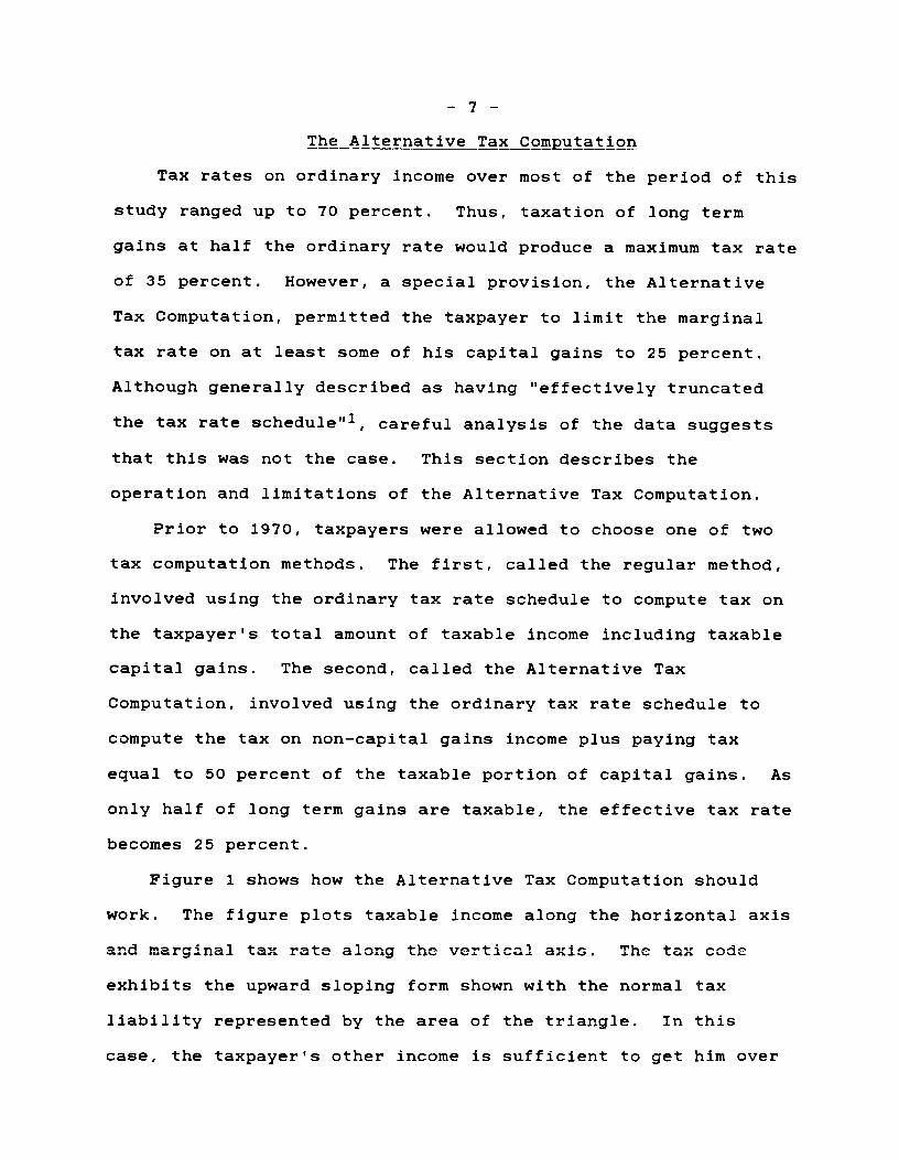
Figure 1 shows how the Alternative Tax Computation should

work. The figure plots taxable income along the horizontal axis

and marginal tax rate along the vertical axis. The tax code

exhibits the upward sloping form shown with the normal tax

liability represented by the area of the triangle. In this

case, the taxpayer's other income is sufficient to get him over

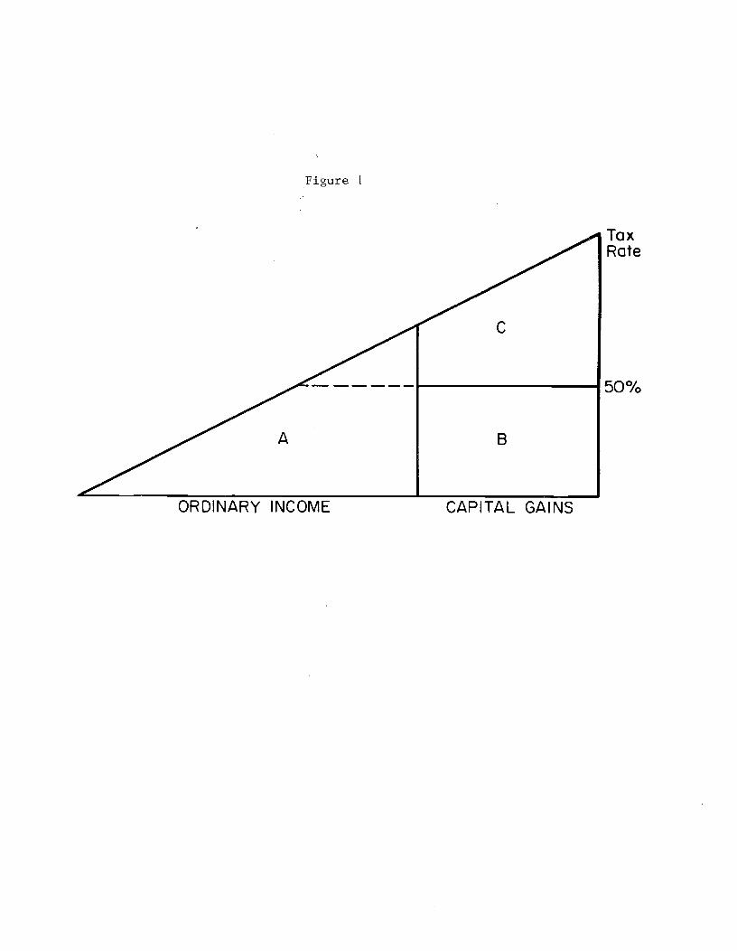
Figure 1

ORDINARY INCOME CAPITAL GAINS

TaxRate

50%

—8—the 50 percent bracket amount, and he pays tax liability

indicated by area A on his ordinary income. In addition, the

taxpayer pays 50 percent on the included portion of capital

gains. This is indicated by area B. The total tax saving to

this taxpayer from the alternative tax computation is area C,

and his marginal tax rate on capital gains is limited to 25

percent.

Now consider the case shown in Figure 2. Here, the

taxpayer's total taxable income is enough to be taxed at a rate

over 50 percent, but his non-capital gains income is not. The

taxpayer has a choice. He can elect to be taxed under the

regular tax rate schedule, in which case his tax liability is

the large triangle , or he can elect the alternative tax

computation. If he chooses the alternate tax computation, tax

is levied by the ordinary schedule on his non-capital gains

income, equal to area D. In addition, he pays tax at a 50

percent rate on the included portion of capital gains, indicated

by areas E and F. As area E indicates, a portion of the

taxpayer's long term gains are taxed at a rate higher than they

would be under the normal tax rate schedule. This taxpayer

elects the alternative tax computation only if it results in a

tax savings. In this case, such a situation results only if

area E is less than area G.

Consider a taxpayer situation where this is the case. The

taxpayer realizes long term gains of $200,000 and has other

income of $50,000. In addition, he has itemized deductions of

$40,000. The taxpayer excludes half of the long term gains from

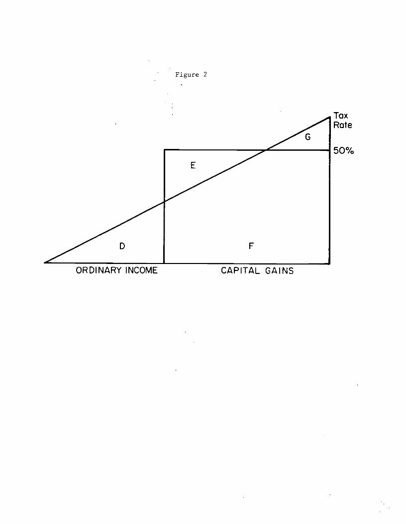
Figure 2

ORDINARY INCOME CAPITAL GAINS

TaxRate

50%

—9—tax, leaving an Adjusted Gross Income of $150,000, and then

subtracts itemized deductions to produce a taxable income of

$110,000. Using the tax schedule of the era (1965-1969), the

ordinary tax computation would produce a tax liability of

$51,380. Under the alternative tax computation, he would pay

ordinary tax on the first $10,000, equal to $1,820, plus a 50

percent tax on the $100,000 of included gains, producing a total

tax liability of $51,820.

This taxpayer would elect to be taxed under the ordinary

schedule as it produces a lower tax liability. However, the

marginal tax rate under this schedule is 62 percent, producing a

marginal tax rate on capital gains of 31 percent. In this case,

the alternative tax computation did not effectively limit the

tax rate on long term gains to 25 percent. An effective tax

rate limit of 25 percent would require that the last $25,000 of

included capital gains be taxed at 50 percent, rather than the

first $25,000.

Although a majority of taxpayers in upper income brackets

who realized long term gains did avail themselves of the

alternative tax computation method, a signficant fraction did

not. For example, in 1966, of 27,766 taxpayers with Adjusted

Gross Incomes between $100,000 and $200,000, more than one

quarter did not elect the alternative tax computation. The same

was true for 16 percent of taxpayers with Adjusted Gross Incomes

between $200,000 and $500,000 with net long term capital gains,

and for 7.5 percent of taxapayers in the same situation with

Adjusted Gross Income over $500,0002.

— 10 —

The data are not sufficient to indicate the reason why these

taxpayers elected the ordinary tax computation. It should be

noted, however, that taxpayers are less likely to chose the

alternative tax computation as long term gains rise as a share

of income. An extreme example would be a taxpayer with negative

ordinary taxable Income but large amounts of positive capital

gains. This could be due to net operating losses in a business

or partnership or to itemized deductions such as state taxes,

interest, and charitable contributions, exceeding his ordinary

income. The ordinary tax computation effectively permits this

taxpayer to shelter that portion of his long term gain which

offsets the negative part of his ordinary taxable income . But,

under the alternative tax computation, the tax on this negative

portion of income would be zero, while the tax on the included

portion of capital gains would be at the full 50 percent rate.

Thus, in certain situations, taxpayers with a substantial

capital gain may still find themselves excluded from the

alternate tax computation. The effect of this on the average

marginal tax rate on taxpayers with net long term gains was an

increase of 1.5 percentage points above the 25 percent

theoretical maximum for taxpayers in the $100,000 to $500,000

income range.

The Tax Reform Act of 1969 changed the alternative tax

computation by limiting the 25 percent rate to a maximum of

$50,000 in net long term gains. Thus, only $25,000 of the

included half of long term gains qualified for the "special" 50

percent rate. In 1970, the excess over this amount was taxed

— 11 —

at a maximum rate of 59 percent. This maximum tax rate was

raised to 65 percent in 1971 and the limit was removed

completely in 1972 and later years.

The actual alternative tax computation was constructed to

minimize the potential benefits to the taxpayer. Figure 3 shows

the method of computation for a taxpayer who would receive some

benefit from the computation. The tax owed was comprised of

three parts. The first part, denoted as area H, was the tax

owed on the taxpayer's ordinary taxable income. This

corresponds to area A in Figure 1. The second part, denoted as

area I, was a 50 percent tax on the first $25,000 of the

included portion of capital gains. If the included portion of

the taxpayer's gains was less than $25,000, then the effective

marginal tax rate on these gains was 25 percent, and no further

computation is necessary. If capital gains exceeded $25,000

then the tax computation included a third part, denoted as area

J. This was the difference between (a) the tax calculated using

the ordinary computation on the taxpayer's total taxable income

and (b) the tax calculated using the ordinary computation on the

sum of $25,000 plus the taxpayer's non-capital gains taxable

income.

If the taxpayer did not elect the alternative tax

computation, his tax would have been the total area under the

ordinary tax schedule, denoted as areas H, I, .1, and K. The net

tax savings to the taxpayer was therefore area K. Note that for

any taxpayer with more than $25,000 of included capital gains,

the marginal tax rate on gains was the same as it would have

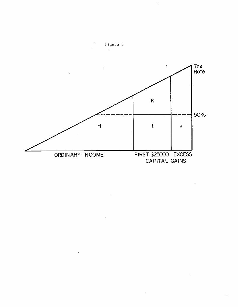
Figure 3

TaxRate

5Q0/

ORDINARY INCOME EXCESSCAPITAL GAINS

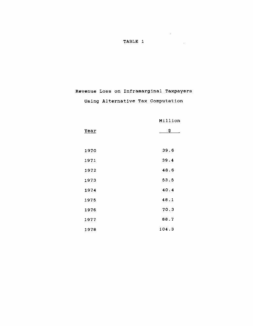
TABLE 1

Revenue Loss on Inframarginal Taxpayers

Using Alternative Tax Computation

Million

Year _______

1970 39.6

1971 39.4

1972 48.6

1973 53.5

1974 40.4

1975 48.1

1976 70.3

1977 88.7

1978 104.3

— 12 —

been had their been no alternative tax computation. Thus, to

the extent that capital gains realizations are based on marginal

incentives, the alternative tax computation had no effect on a

substantial number of taxpayers. Table 1 provides estimates of

the revenue loss from this provision of an inframarginal tax

reduction to recipients of capital gains.

The change in the alternative tax computation to limit

special treatment to only $25,000 of included gains also had the

effect of lowering the fraction of taxpayers electing the

alternative computation, even among taxpayers with more than

$25,000 of capital gains. Figure 4 shows a taxpayer situation

in which it may not be in the interest of the taxpayer to elect

the alternative tax computation. The taxpayer must pay tax

above the statutory rate on a portion of his gains in the hopes

that this will offset a lower rate on some of the rest of his

gains. This taxpayer would owe tax equal to areas L, M, N, and

0. Under the ordinary tax computation he would owe taxes on L,

M, 0, and P. The taxpayer thus elects the alternative tax

computation only if area N is smaller than area P.

The effect of this change in the alternative computation was

to limit the marginal incentive to a minority of taxpayers in

income groups with high marginal rates. Table 2 shows the

fraction of taxpayers in high income groups with net long term

capital gains who did not receive a marginal benefit from the

alternative tax computation and the reason why. In only one

income group in one year did a majority receive a marginal rate

reduction.

— 13 —

There are two reasons for this ineffectiveness. First, it

was impossible for any taxpayer with more than $25,000 in gains

to benefit at the margin. Second, taxpayers with relatively

small amounts of non—capital gains taxable income would also not

benefit regardless of the size of their capital gains income.

This limited alternative tax computation was therefore of

marginal benefit only to taxpayers with relatively small amounts

of capital gains income and relatively large amounts of other

income. However, as noted above, much of the effect was infra-

marginal with regard to taxpayer decision making, while costing

significant amounts of revenue.

The Additional Minimum Tax

The Tax Reform Act of 1969 began the Additional Tax for Tax

Preferences, also known as the minimum tax. The excluded

portion of capital gains was among a list of 9 types of income,

termed preferences, which came under the minimum tax. The

additional minimum tax was levied in two forms, one from 1970

through 1975, and one from 1976 through 1978. We consider each

in turn.

The early form of the tax was levied at a 10 percent rate on

the items of tax preference reduced by an exclusion of $30,000

plus the taxpayer's ordinary tax liability and some other

deductions discussed later. The effect of this was to make the

taxpayer's additional tax rate negatively related to his

ordinary tax rate. In the case of the capital gains tax

preference, the additional tax rate was negatively related to

— 14 —

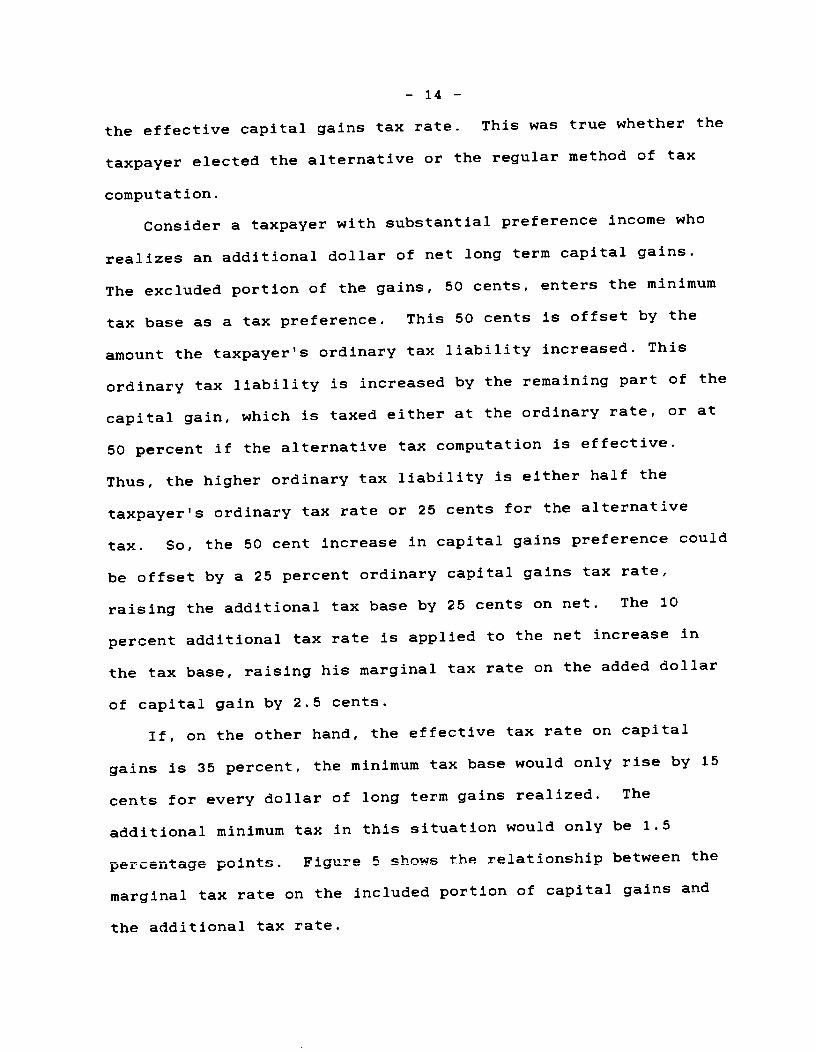
the effective capital gains tax rate. This was true whether the

taxpayer elected the alternative or the regular method of tax

computation.

Consider a taxpayer with substantial preference income who

realizes an additional dollar of net long term capital gains.

The excluded portion of the gains, 50 cents, enters the minimum

tax base as a tax preference. This 50 cents is offset by the

amount the taxpayer's ordinary tax liability increased. This

ordinary tax liability is increased by the remaining part of the

capital gain, which is taxed either at the ordinary rate, or at

50 percent if the alternative tax computation is effective.

Thus, the higher ordinary tax liability is either half the

taxpayer's ordinary tax rate or 25 cents for the alternative

tax. So, the 50 cent increase in capital gains preference could

be offset by a 25 percent ordinary capital gains tax rate,

raising the additional tax base by 25 cents on net. The 10

percent additional tax rate is applied to the net increase in

the tax base, raising his marginal tax rate on the added dollar

of capital gain by 2.5 cents.

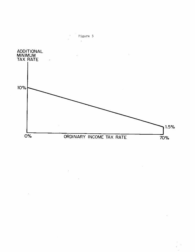
If, on the other hand, the effective tax rate on capital

gains is 35 percent, the minimum tax base would only rise by 15

cents for every dollar of long term gains realized. The

additional minimum tax in this situation would only be 1.5

percentage points. Figure 5 shows the relationship between the

marginal tax rate on the included portion of capital gains and

the additional tax rate.

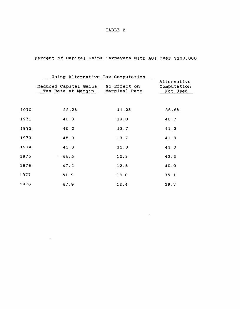
TABLE 2

Percent of Capital Gains Taxpayers With AGI Over $100,000

1970

1971

1972

1973

1974

1975

1976

1977

_ng_Alternative

Reduced Capital GainsTax Rate at Main

22.2%

40.3

45.0

45.0

41.3

44 . 5

47.2

51.9

_C omputat ion

No Effect onMarginal Rate

41.2%

19.0

13.7

13.7

11.3

12.3

12.8

13.0

AlternativeComputationNot Used

36.6%

40.7

41.3

41.3

47.3

43 . 2

40 . 0

35.1

1978 47.9 12.4 39.7

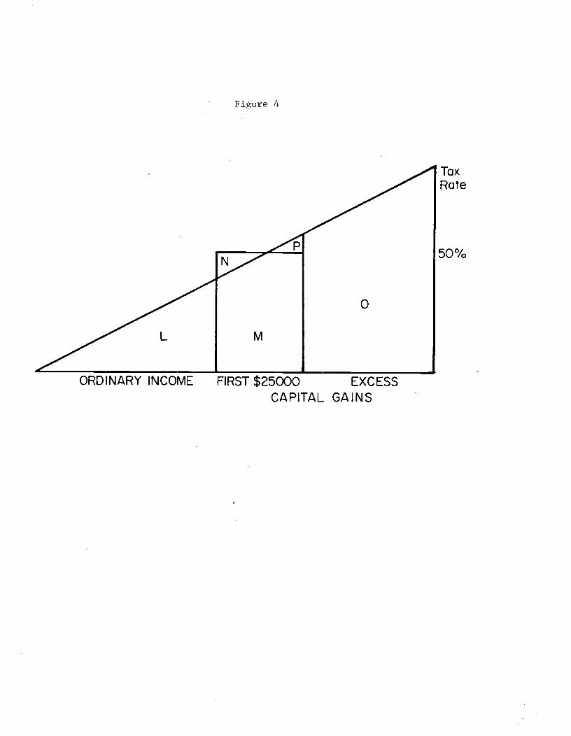
Figure 4

TaxRate

50%

ORDINARY INCOME FIRST $25000 EXCESSCAPITAL GAINS

— 15 —

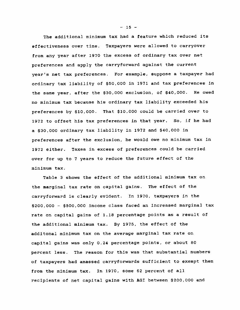
The additional minimum tax had a feature which reduced its

effectiveness over time. Taxpayers were allowed to carryover

from any year after 1970 the excess of ordinary tax over net

preferences and apply the carryforward against the current

yeares net tax preferences. For example, suppose a taxpayer had

ordinary tax liability of $50,000 in 1971 and tax preferences in

the same year, after the $30,000 exclusion, of $40,000. He owed

no minimum tax because his ordinary tax liability exceeded his

preferences by $10,000. That $10,000 could be carried over to

1972 to offset his tax preferences in that year. So, if he had

a $30,000 ordinary tax liability in 1972 and $40,000 in

preferences after the exclusion, he would owe no minimum tax in

1972 either. Taxes in excess of preferences could be carried

over for up to 7 years to reduce the future effect of the

minimum tax.

Table 3 shows the effect of the additional minimum tax on

the marginal tax rate on capital gains. The effect of the

carryforward is clearly evident. In 1970, taxpayers in the

$200,000 — $500,000 income class faced an increased marginal tax

rate on capital gains of 1.18 percentage points as a result of

the additional minimum tax. By 1975, the effect of the

additonal minimum tax on the average marginal tax rate on

capital gains was only 0.24 percentage points, or about 80

percent less. The reason for this was that substantial numbers

of taxpayers had amassed carryforwards sufficient to exempt them

from the minimum tax. In 1970, some 62 percent of all

recipients of net capital gains with AGI between $200,000 and

ADDITIONALMINIMUMTAX RATE

lf'o,ILl /0

Figure 5

I O/I.._) 10

0% ORDINARY INCOME TAX RATE 70%

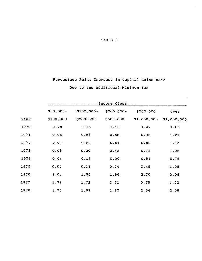
TABLE 3

Percentage Point Increase in Capital Gains Rate

Due to the Additional Minimum Tax

Income Class

$50,000— $100,000— $200,000— $500,000 over

Year $1 00000 $200, 000 $SOQLQOO i1OQ000 00000O1970 0.28 0.75 1.18 1.47 1.65

1971 0.08 0.26 0.58 0.98 1.27

1972 0.07 0.22 0.51 0.80 1.15

1973 0.06 0.20 0.42 0.72 1.02

1974 0.04 0.15 0.30 0.54 0.75

1975 0.04 0.11 0.24 0.45 1.08

1976 1.04 1.56 1.96 2.70 3.08

1977 1.37 1.72 2.21 3.75 4.62

1978 1.35 1.69 1.87 2.34 2.66

— 16 —

$500,000 paid some additional tax. By 1975, only 13 percent of

capital gains recipients in the same income category paid the

additional tax.

The Tax Reform Act of 1976 made substantial changes in the

minimum tax which greatly increased its scope. The carryforward

from previous years was ended altogether. Two additional

preferences were added, one for intangible drilling costs and

one for itemized deductions in excess of 60 percent of Adjusted

Gross Income. The tax rate was raised to 15 percent and the

exclusion lowered to the greater of $10,000 or one half of

ordinary tax liability. The IRS estimates3 that this resulted

in an eleven fold increase in the number of taxpayers paying the

minimum tax and a six fold increase in minimum tax revenues.

The 1976 changes in the minimum tax raised the average

effective tax rate on capital gains in two ways. First, it

increased the number of taxpayers subject to the additional levy

of the minimum tax, as the above figures indicate. Second, it

increased the addition to the effective tax rate caused by the

minimum tax for each minimum taxpayer. Figure 6 illustrates how

this new minimum tax affected the marginal tax rate on capital

gains.

If a taxpayer received an additional dollar of net long term

capital gains, the 50 cents excluded from the ordinary tax was

treated as a tax preference. The remaining 50 cents raised the

ordinary tax the taxpayer paid. Half of the increase in

ordinary tax was used as an offset against preference income

rather than the full amount of ordinary tax as in the 1969 law.

ADDITIONALMINIMUMTAX RATE15

Figure 6

4.875%

70%

— 17 —

So, if the taxpayer were In the 50 percent tax bracket, the

additional dollar of capital gains would raise his ordinary

taxes by 25 cents and his offset by 12.5 cents. In this case,

the taxpayer's additional minimum tax base would rise by 37.5

cents. This base is taxed at a 15 percent rate, meaning that

the taxes paid on the additional dollar of capital gains Is

increased by 5.625 cents.

As was the case before 1976, the additional taxes paid fall

as the taxpayer's ordinary marginal tax rate rises. If a

taxpayer's ordinary tax rate was 70 percent and the alternative

tax computation was not effective at the margin, the ordinary

tax would rise by 35 cents for every dollar of capital gains

realized. This would mean a 17.5 cent offset against the

additional 50 cents in tax preferences. The resulting 32.5 cent

Increase in the minimum tax base means that the minimum tax

raised the effective tax rate on capital gains by 4.875 cents.

The additional tax had its greatest effect on the marginal

tax rate on capital gains in 1977. In that year it raised the

average capital gains rate in the top bracket by 4.6 percentage

points. Some 92 percent of capital gains recipients with AGI

over $1,000,000 were subject to the additional minimum tax in

that year. The effect of the additional tax was much less in the

top brackets In 1978. In that year only 52 percent of the

recipients of capital gains in the over $1,000,000 income group

paid additional tax. The reason for this is probably the tax

legislation which moved through Congress that year. The

additional minimum tax was eliminated beginning in January,

— 18 —

1979. Tax conscious investors may well have postponed their

realizations to take account of this (and other) changes in the

tax law which had the effect of lowering the capital gains tax

rate.

The additional minimum tax interacted with other provisions

of the tax code. As already noted, taxpayers electing the

alternative tax computation would face higher additional minimum

taxes on their capital gains than taxpayers who computed their

tax according to the regular tax rate schedule. The additional

minimum tax also interacted with the Maximum Tax on Personal

Service Income in a manner which increased the effective tax

rate on capital gains income.

Maximum Tax on Personal Service Income

The Maximum Tax on Personal Service Income, otherwise known

as the "maximum tax" was enacted as part of the Tax Reform Act

of 1969. Its objective was to reduce the effective tax rate on

wage, salary, and professional income below that on other types

of income. Instead of the statutory 70 percent top rate, the

top rate on personal service income was set at 60 percent in

1971 and 50 percent thereafter. As Lindsey (1981) showed, the

maximum tax was ineffective at achieving these objectives for

the vast majority of high income taxpayers. However, a complex

interaction between the maximum tax and other provisions of the

tax law had the effect of raising the effective capital gains

tax rate for many taxpayers.

— 19 —

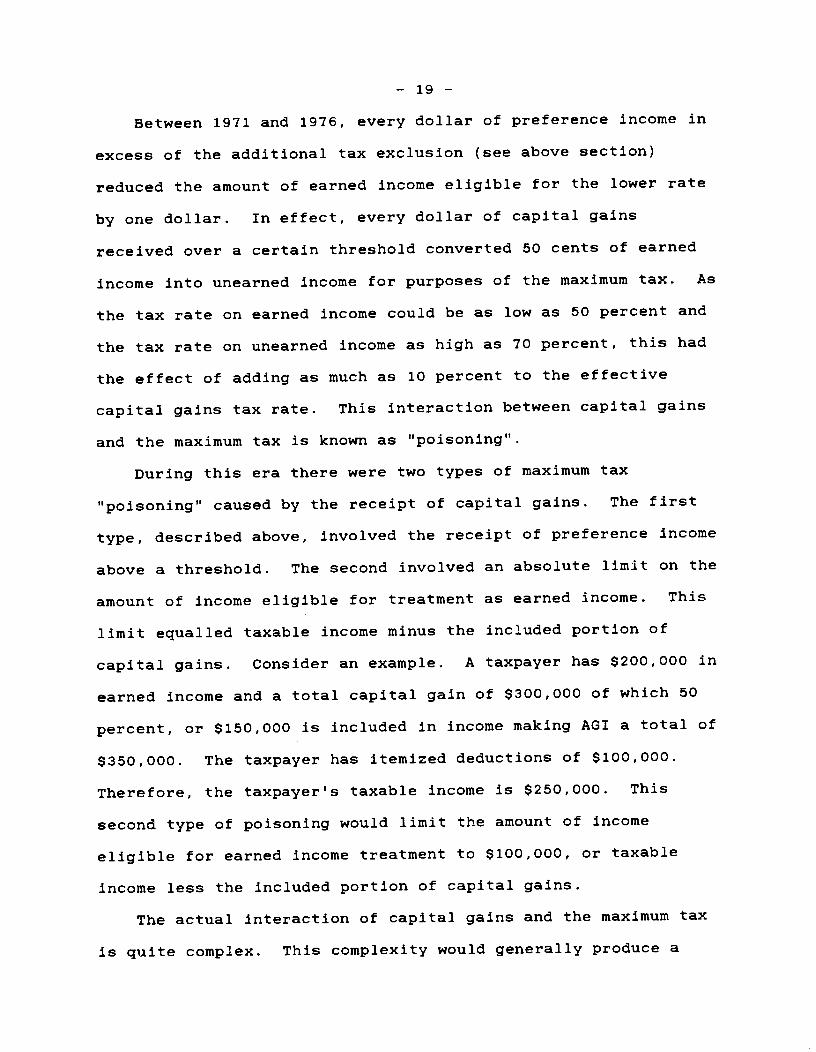
Between 1971 and 1976, every dollar of preference income in

excess of the additional tax exclusion (see above section)

reduced the amount of earned income eligible for the lower rate

by one dollar. In effect, every dollar of capital gains

received over a certain threshold converted 50 cents of earned

income into unearned income for purposes of the maximum tax. As

the tax rate on earned income could be as low as 50 percent and

the tax rate on unearned income as high as 70 percent, this had

the effect of adding as much as 10 percent to the effective

capital gains tax rate. This interaction between capital gains

and the maximum tax is known as "poisoning".

During this era there were two types of maximum tax

"poisoning" caused by the receipt of capital gains. The first

type, described above, involved the receipt of preference income

above a threshold. The second involved an absolute limit on the

amount of income eligible for treatment as earned income. This

limit equalled taxable income minus the included portion of

capital gains. Consider an example. A taxpayer has $200,000 in

earned income and a total capital gain of $300,000 of which 50

percent, or $150,000 is included in income making AGI a total of

$350,000. The taxpayer has itemized deductions of $100,000.

Therefore, the taxpayer's taxable income is $250,000. This

second type of poisoning would limit the amount of income

eligible for earned income treatment to $100,000, or taxable

income less the included portion of capital gains.

The actual interaction of capital gains and the maximum tax

is quite complex. This complexity would generally produce a

— 20 —

rate of "poisoning" slightly lower than that described above.

The amount of income eligible for treatment as earned income,

known as Earned Taxable Income (ETI) is given by the following

formula:

(1) ETI = (PSINC/AGI) X TAXINC - PREFERENCES

In this equation PSINC, or personal service income, equals

income from wages, salaries, and professional income. TAXINC,

or taxable income, is apportioned between earned and unearned

portions according to the share of AGI contributed by PSINC.

Earned Taxable Income is then reduced by the amount of

preference income, including the excluded portion of capital

gains. This latter substraction represents the "poisioning"

effect described above.

However, the derivative of earned taxable income with

respect to a change in capital gains shows that there is a an

offset to this poisoning as well:

(2) dETI = 0.5 PS CjAGI-TAXINCj - 0.5dCAPGN AGI2

— 21 —

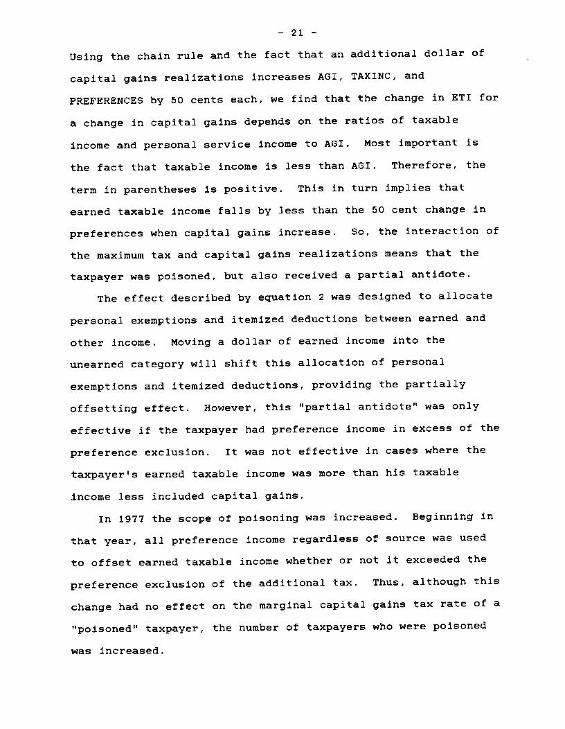
Using the chain rule and the fact that an additional dollar of

capital gains realizations increases AGI, TAXINC, and

PREFERENCES by 50 cents each, we find that the change in ETI f or

a change in capital gains depends on the ratios of taxable

income and personal service income to AGI. Most important is

the fact that taxable income is less than AGI. Therefore, the

term in parentheses is positive. This in turn implies that

earned taxable income falls by less than the 50 cent change in

preferences when capital gains increase. So, the interaction of

the maximum tax and capital gains realizations means that the

taxpayer was poisoned, but also received a partial antidote.

The effect described by equation 2 was designed to allocate

personal exemptions and itemized deductions between earned and

other income. Moving a dollar of earned income into the

unearned category will shift this allocation of personal

exemptions and itemized deductions, providing the partially

offsetting effect. However, this "partial antidote" was only

effective if the taxpayer had preference income in excess of the

preference exclusion. It was not effective in cases where the

taxpayer's earned taxable income was more than his taxable

income less included capital gains.

In 1977 the scope of poisoning was increased. Beginning in

that year, all preference income regardless of source was used

to offset earned taxable income whether or not it exceeded the

preference exclusion of the additional tax. Thus, although this

change had no effect on the marginal capital gains tax rate of a

"poisoned" taxpayer, the number of taxpayers who were poisoned

was increased.

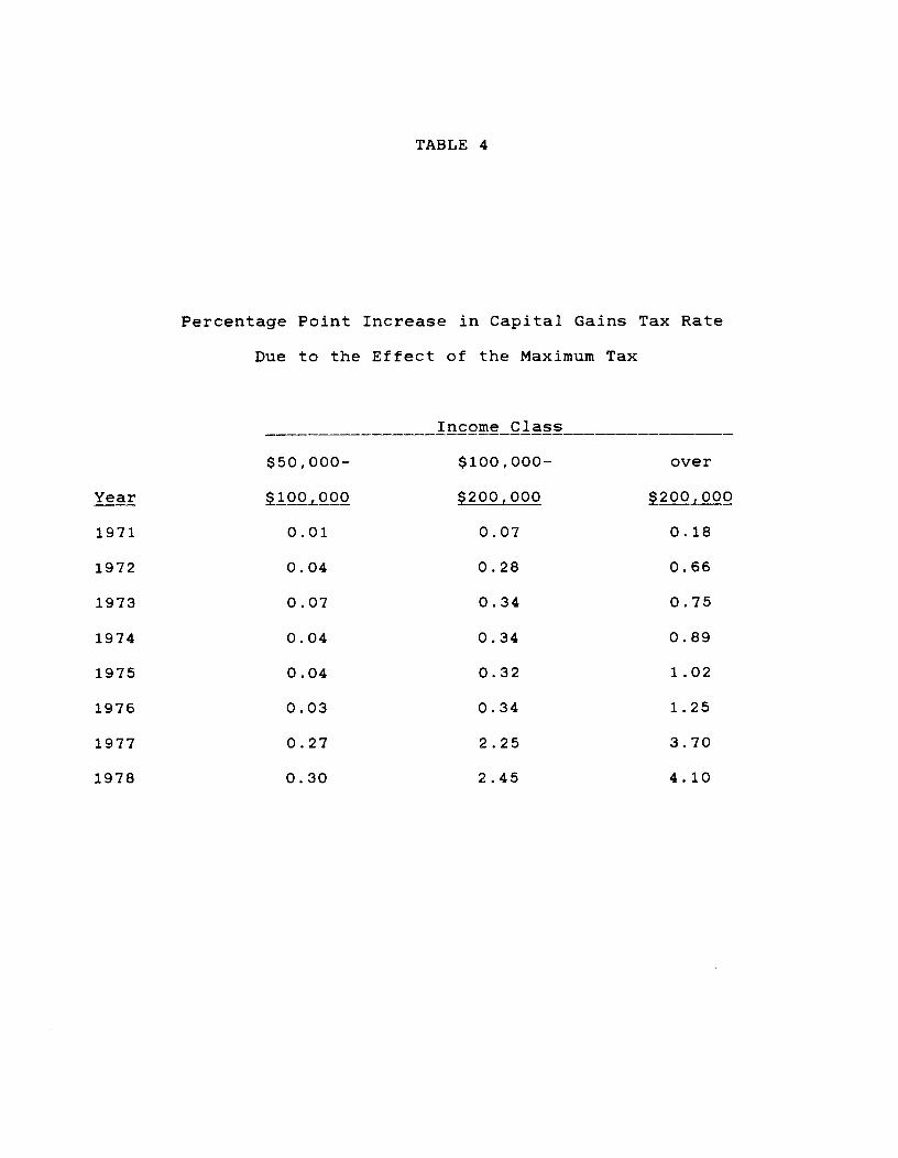
TABLE 4

Percentage Point Increase in Capital Gains Tax Rate

Due to the Effect of the Maximum Tax

____ ____ Income Class ______

$50,000- $100,000- over

Year 4Q0L0O0 200 000 20000O

1971 0.01 0.07 0.18

1972 0.04 0.28 0.66

1973 0.07 0.34 0.75

1974 0.04 0.34 0.89

1975 0.04 0.32 1.02

1976 0.03 0.34 1.25

1977 0.27 2.25 3.70

1978 0.30 2.45 4.10

— 22 —

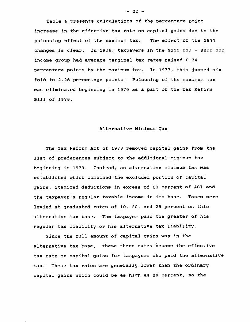
Table 4 presents calculations of the percentage point

increase in the effective tax rate on capital gains due to the

poisoning effect of the maximum tax. The effect of the 1977

changes is clear. In 1976, taxpayers in the $100,000 — $200,000

income group had average marginal tax rates raised 0.34

percentage points by the maximum tax. In 1977, this jumped six

fold to 2.25 percentage points. Poisoning of the maximum tax

was eliminated beginning in 1979 as a part of the Tax Reform

Bill of 1978.

Alternative Minimum_Tax

The Tax Reform Act of 1978 removed capital gains from the

list of preferences subject to the additional minimum tax

beginning in 1979. Instead, an alternative minimum tax was

established which combined the excluded portion of capital

gains, itemized deductions in excess of 60 percent of AGI and

the taxpayerts regular taxable income in its base. Taxes were

levied at graduated rates of 10, 20, and 25 percent on this

alternative tax base. The taxpayer paid the greater of his

regular tax liability or his alternative tax liability.

Since the full amount of capital gains was in the

alternative tax base, these three rates became the effective

tax rate on capital gains for taxpayers who paid the alternative

tax. These tax rates are generally lower than the ordinary

capital gains which could be as high as 28 percent, so the

— 23 —

alternative minimum tax had the effect of lowering the marginal

tax rate on capital gains, even though the average tax rate paid

by alternative minimum taxpayers was increased by the provision.

Nearly all alternative minimum taxpayers with AGI over

$200,000 paid taxes at the 25 percent effective tax rate. In

the $100,000 — $200,000 income class this fell to about three

fourths of taxpayers paying the alternative minimum tax, with

the average alternative minimum rate in this group at 23.6

percent. The average rate was only 17.6 percent in the $50,000

— $100,000 income group.

The net result of the alternative minimum tax was to reduce

the average marginal tax rate on capital gains in the top income

groups by about one percentage point in 1979, and about 0.4

percentage points in 1980. But, because the top regular capital

gains rate averaged 24 percent in 1981, the effect of the

minimum tax was to increase the average marginal tax rate by

about 0.2 percentage points that year. Other income groups had

tax rate changes of about 0.2 percentage points as a result of

the alternative minimum tax.

The Economic Recovery Tax Act of 1981 eliminated the 25

percent tax bracket on the Alternative Minimum Tax. This meant

that beginning in 1982, alternative minimum taxpayers faced the

same effective tax rate on capital gains as ordinary taxpayers

—— 20 percent.

— 24 —

Combined_Effects

Table 5 presents calculations of the average effective tax

rate faced by taxpayers with net long term gains in excess of

short term losses. The calculations were based on the tax

computation status of taxpayers with such gains as reported in

the Statistics onc. The calculations weighted all

taxpayers equally within a given income class in order to

minimize the simultaneity between the tax rate and the level of

realizations. The tax rate estimates include the effects of the

interactions between the various types of taxation described in

this section.

Also included in the tax rate estimates are the effects of

the changes in the exclusion rate in the 1978 tax bill and the

maximum capital gains rate in the 1981 tax bill. The 1978 act

increased the rate of exclusion of net long term gains from 50

percent to 60 percent for all assets sold after October 31,

1978. The figures for 1978 therefore take a weighted average of

tax rates implied by the two exclusion rates in proportion to

the fraction of the year each exclusion rate was in effect. In

other words, a weight of .833 was attached to the rates

applicable to a 50 percent exclusion and a weight of .167 was

attached to the rates applicable to a 60 percent exlcusion.

The Economic Recovery Tax Act of 1981 reduced the maximum

tax rate on capital gains to 20 percent for all assets sold

after June 9, 1981. The 1981 rates therefore reflect a weighted

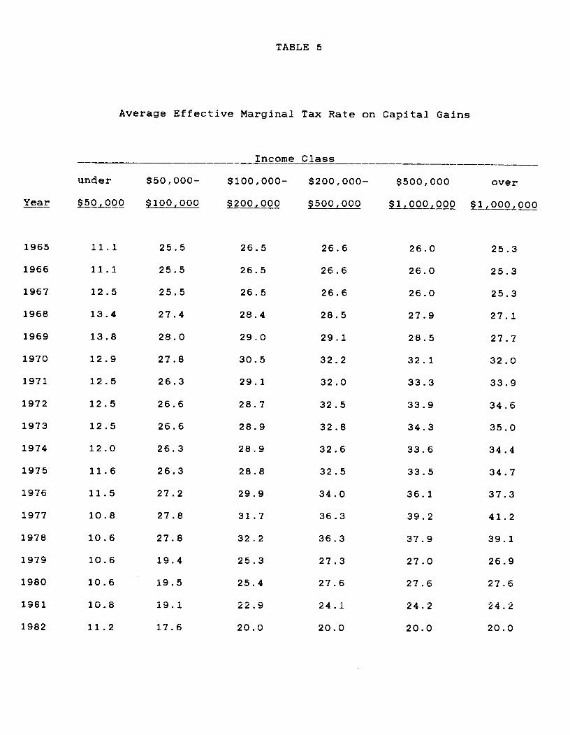
TABLE 5

Average Effective Marginal Tax Rate on Capital Gains

under

$5 0 000

$50,000—

.10o, 000

Income Class

$100,000— $200,000— $500,000 over

200 000 00L000 1000000 iQQpQOYear

1965 11.1 25.5 26.5 26.6 26.0 25.3

1966 11.1 25.5 26.5 26.6 26.0 25.3

1967 12.5 25.5 26.5 26.6 26.0 25.3

1968 13.4 27.4 28.4 28.5 27.9 27.1

1969 13.8 28.0 29.0 29.1 28.5 27.7

1970 12.9 27.8 30.5 32.2 32.1 32.0

1971 12.5 26.3 29.1 32.0 33.3 33.9

1972 12.5 26.6 28.7 32.5 33.9 34.6

1973 12.5 26.6 28.9 32.8 34.3 35.0

1974 12.0 26.3 28.9 32.6 33.6 34.4

1975 11.6 26.3 28.8 32.5 33.5 34.7

1976 11.5 27.2 29.9 34.0 36.1 37.3

1977 10.8 27.8 31.7 36.3 39.2 41.2

1978 10.6 27.8 32.2 36.3 37.9 39.1

1979 10.6 19.4 25.3 27.3 27.0 26.9

1980 10.6 19.5 25.4 27.6 27.6 27.6

1981 10.8 19.1 22.9 24.1 24.2 24.2

1982 11.2 17.6 20.0 20.0 20.0 20.0

— 25 —

average of rates which ranged up to the old maximum of 28

percent for half the year and 20 percent for the other half the

year. In this case, equal weights were attached to the two tax

rate scenarios.

The data show that the maximum capital gains tax rate

increased rapidly between 1967 and 1977 and decreased rapidly

thereafter. These data provide a significant amount of variance

in the tax rate term. The next section describes how these data

were combined with data on wealth to estimate the sensitivity of

taxpayers to changes in the capital gains tax rate.

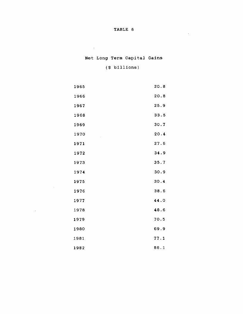
TABLE 6

Net Long Term Capital Gains

($ billions)

1965 20.8

1966 20.8

1967 25.9

1968 33.5

1969 30.7

1970 20.4

1971 27.6

1972 34.9

1973 35.7

1974 30.9

1975 30.4

1976 38.6

1977 44.0

1978 48.6

1979 70.5

1980 69.9

1981 77.1

1982 86.1

— 26 —

II.

The level of capital gains realizations has trended upward

throughout the period of this study, 1965-1982. Table 6

presents the nominal value of net long term capital gains

realizations in each of the 18 years encompassed by this study.

Net long term realizations in 1982 were more than 4 times their

1965 level. In 13 of the 18 years capital gains were higher

than in the preceding year.

This general upward trend was marked by a number of

discontinuities. Capital gains in 1969 and 1970 were well below

the values of 1968. Net realizations were also lower in 1974

and 1975 than In 1973. 1969 and 1970 were associated with

higher tax rates than preceding years due to the Vietnam War

surtax. 1970 was associated with a decline in the stock market.

1974 and 1975 were also associated with a declining stock

market.

On the other hand, very rapid growth in capital gains

realizations occurred between 1978 and 1979. Net long term

gains in 1979 were 45 percent greater than in 1978. 1979 was

associated with only a very modest advance in stock prices,

however. The sharp decline in capital gains tax rates appears

to be a primary factor in this advance in realizations. Capital

gains realizations in 1978 may also have been depressed in

anticipation of the cuts in 1979, increasing the apparent

percentage rise in realizations.

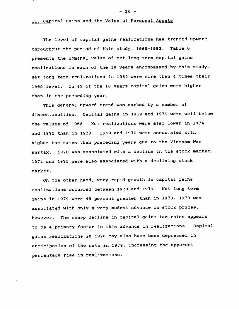
— 27 —

The debate over the importance of capital gains rates in

determining realizations is complicated by changes in the value

of personal wealth including accrued but unrealized capital

gains. The objective of this section is to estimate values for

personal wealth holdings in order to control for this factor in

determining the role that capital gains tax rates play in

realizations.

The Federal Reserve Board issues a quarterly Flow of Funds

report on the holdings of various sectors of the U.S. economy.

These figures contain detailed balance sheets and reconciliation

statements for the asset holdings of households, government, and

corporations. The present study uses the values of wealth

holdings by households.

The components of household wealth include many elements on

which households either cannot or probably will not realize

capital gains. For example, holdings of cash, checking and

savings deposits do not include the possibility of capital

gains. Capital gains accruing to households via financial

intermediaries such as life insurance and pension funds are also

not reported as capital gains when the taxpayer files his tax

return. Capital gains in pension funds, including IRA and Keogh

accounts, are reported as pension income when the funds are

dispersed after retirement.

We therefore chose to divide household wealth into two

components: those readily tradeable and subject to potential

capital gains realizations, and those unlikely to be subject to

such realizations. This section considers each in turn.

— 28 —

Tradeable Wealth

Tradeable wealth is comprised of those assets on which

capital gains are regularly realized. The Internal Revenue

Service has tabulated the distribution of capital gains by type

of asset. Table 7 provides the percentage breakdown of sales of

capital assets by the number of transactions and the value of

net gains. The data show that sales of corporate stock, real

estate, and capital gains income which passes through to the

individual taxpayer from small business corporations

proprietorships1 and partnerships comprise some 97 percent of

the value of net capital gains.

In the context of the data in the Flow of Funds, these

categories include land, residential structures, corporate

equities, and equity in non-corporate businesses. This latter

category includes the value of non—residential real estate held

by households. Tangible assets such as consumer durables on

which capital gains are rarely reported, were excluded from this

study.

These traded assets have tended to comprise about two thirds

of all household wealth over the period studied. This share

varied from a high of 69 percent in 1968 to a low of 65 percent

in 1975. The most variable component of this traded wealth is

household holdings of corporate equities which fell from nearly

23 percent of total wealth in 1968 to only 9.5 percent in 1979.

The rapid decline in the holding of corporate equity was offset

— 29 —

by increased holding of real estate. Non-residential real

estate peaked at 39.4 percent of household wealth in 1979, up

from a low of 28 percent at the beginning of the period being

studied.

Due to this variation in the components of personal wealth

over time, we apportioned household wealth among the six income

groups studied on a component by component basis. Each

component was allocated according to the distribution of income

reported on tax returns likely to flow from that component of

household wealth. For example, the distribution of corporate

equities in a given year was assumed to be the same as the

distribution of dividends in that year. The sum of net rental

income and net rental loss was used to apportion real estate

wealth. Non—corporate business wealth was apportioned by

summing net profits and net losses from proprietorships,

partnerships, and small business corporations.

The key advantage of this apportioning technique was that

the shares of wealth were determined from the same data base as

the data on the level and distribution of capital gains

realizations, Observations on individual income classes in each

year were therefore independent of observations from other

years. Capital gains income was excluded from the apportionment

process to avoid simultaneity. At the same time, the aggregate

level of wealth was determined independently of the data on

capital gains realizations. Table 8 presents the level of

tradeable wealth for each income class in each year of the

period studied.

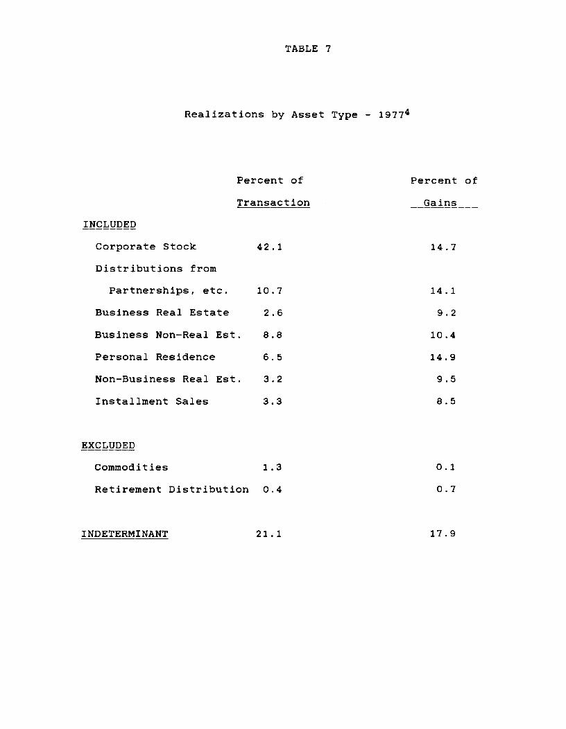
TABLE 7

Realizations by Asset Type — j9774

Percent of Percent of

Transaction Gains

INCLUDED

Corporate Stock 42.1 14.7

Distributions from

Partnerships, etc. 10.7 14.1

Business Real Estate 2.6 9.2

Business Non—Real Est. 8.8 10.4

Personal Residence 6.5 14.9

Non—Business Real Est. 3.2 9.5

Installment Sales 3.3 8.5

EXCLUDED

Commodities 1.3 0.1

Retirement Distribution 0.4 0.7

I NDE TERMINANT 21 . 1 17 . 9

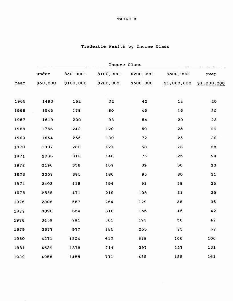
TABLE 8

Tradeable Wealth by Income Class

______ _____________ Income Class _________________

under $50,000— $100,000— $200,000— $500,000 over

Year $50L000 $100000 200000 00, 000 ____ QLQ.Q

1965 1493 162 72 42 14 20

1966 1545 178 80 46 16 20

1967 1619 200 93 54 20 23

1968 1766 242 120 69 25 29

1969 1864 266 130 72 25 30

1970 1907 280 127 68 23 28

1971 2036 313 140 75 25 29

1972 2196 358 167 89 30 33

1973 2307 395 186 95 30 31

1974 2403 419 194 93 28 25

1975 2555 471 219 105 31 29

1976 2806 557 264 129 38 36

1977 3090 654 310 155 45 42

1978 3459 791 381 193 56 47

1979 3877 977 485 255 75 67

1980 4271 1204 617 338 106 108

1981 4659 1378 714 397 127 131

1982 4958 1455 771 455 155 161

— 30 —

One potential criticism of this approach is the allocation

of corporate equity on the basis of dividends received. If

clientele effects exist which are based on tax rates, this

approach would tend to underestimate the value of corporate

equities held by upper income groups since these groups keep a

smaller portion of their dividends after tax relative to capital

gains, than do other goups. However, an upward revaluation of

wealth in upper income groups to reflect this possibility would

put downward pressure on the realizations to wealth ratio among

taxpayer groups with high marginal tax rates. This would in turn

suggest a greater impact of capital gains tax rates on

realizations. We elected to ignore possible clientele effects

in order to err on the side of conservatism in estimating the

effects of capital gains tax rates.

The flow of funds data also includes reconciliation

statements which explain the change in sectoral asset holdings

from year to year. Holdings of a particular asset could vary

for one of two reasons: net purchases or sales of the asset by

the household sector or a change in the price of the existing

stock of holdings. This latter effect is termed "revaluation."

and for purposes of this study was used as a measure of

unrealized capital gains on assets held by households.

We allocated the revaluation of each asset in the same

manner as the stock of wealth held in that asset. Revaluation

values were computed for holding periods up to seven years.

These were converted into inflation adjusted terms by increasing

the nominal value of the asset held at the beginning of the

— 31 —

revaluation period to reflect prices at the end of the

revaluation period. A real value was obtained by subtracting

this from what the value of the assets held at the end of the

revaluation would have been if no net purchases had been made.

In practice, revaluation periods over one year turned out not to

be significant in estimating the level of capital gains. The

data suggested that much of these multi-year revaluations was

picked up in the value of wealth.

Non-traded Wealth

Non—traded wealth was comprised mainly of cash, interest

bearing financial assets, and life insurance and pension fund

reserves. Over the period being studied, pension and life

insurance reserves remained a roughly constant share of

household wealth at about 11 percent. Cash and checking

accounts declined from a bit over 3 percent of wealth to a bit

under 3 percent. Interest bearing financial assets tended to

absorb any fluctuations in the share of non—traded wealth in

total wealth.

As in the case of traded assets, we allocated these

non—tradeable assets on a component by component basis as well.

Cash and checking accounts were allocated in proportion to

Adjusted Gross Income. Interest bearing financial assets were

allocated in proportion to interest income. Pension and life

insurance reserves were allocated in proportion to the sum of

interest and dividend income.

— 32 —

Again, the key advantage of this apportioning technique was

that the shares of wealth were determined from the same data

base as the level and distribution of capital gains.

Independence of observations for individual income classes in

each year was maintained. And, the aggregate level of wealth

was determined independently of the data on capital gains

realizations.

No revaluations of non—traded assets was necessary.

Revaluation of cash, checking, and saving deposits is

impossible. The flow of funds accounts do not provide

revaluations for any interest bearing assets, maintaining each

priced at par. Although some degree of revaluation may actually

have occurred due to fluctuating interest rates, it is likely to

have been quite small. All credit market instruments comprised

only 9 percent of of total financial assets in 1982. This

included short duration assets such as commercial paper on which

no capital gain or loss was likely.

The next section uses this data on the level and

distribution of household wealth in estimating the determinants

of capital gains realizations. Wealth and revaluation values

for given years were obtained by averaging the values at the

beginning and at the end of the year. All of the values f or

wealth and revaluations were converted into real terms using the

average value of the GNP deflator for the year in question.

— 33 —

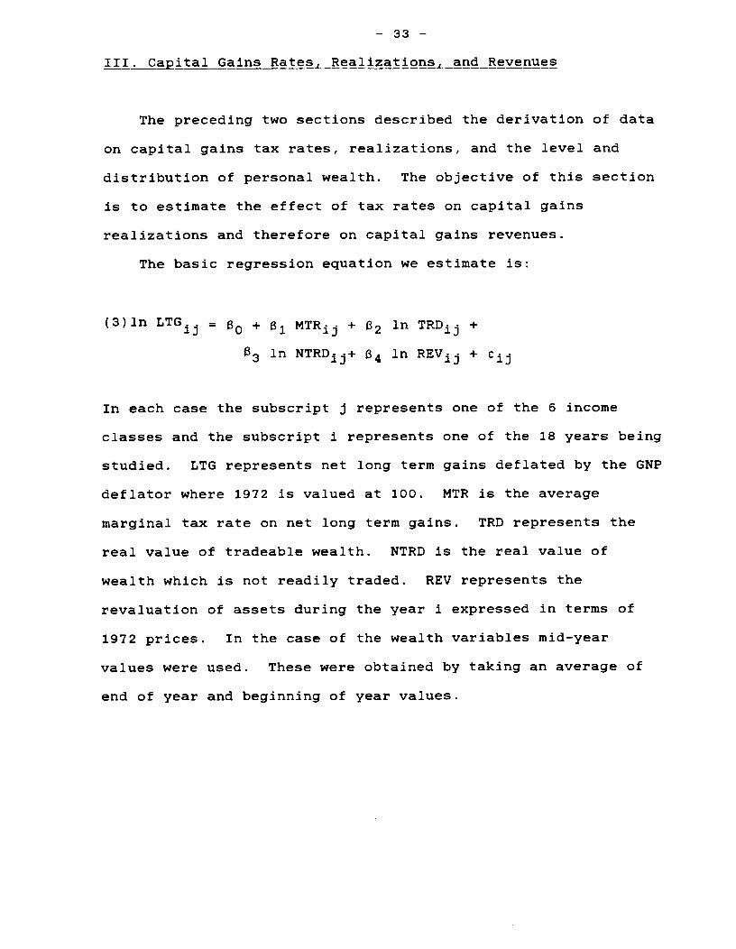
III. Cita 1 Gains Rates Rea]. izations and Revenues

The preceding two sections described the derivation of data

on capital gains tax rates, realizations, and the level anddistribution of personal wealth. The objective of this section

is to estimate the effect of tax rates on capital gains

realizations and therefore on capital gains revenues.

The basic regression equation we estimate is:

(3)ln LTG1 = + MTR1 + B2 in TRD11 +

in NTRD1+ l3 in REV1 +

In each case the subscript j represents one of the 6 income

classes and the subscript i represents one of the 18 years being

studied. LTG represents net long term gains deflated by the GNP

deflator where 1972 is valued at 100. MTR is the average

marginal tax rate on net long term gains. TRD represents the

real value of tradeabie wealth. NTRD is the real value of

wealth which is not readily traded. REV represents the

revaluation of assets during the year i expressed in terms of

1972 prices. In the case of the wealth variables mid—year

values were used. These were obtained by taking an average of

end of year and beginning of year values.

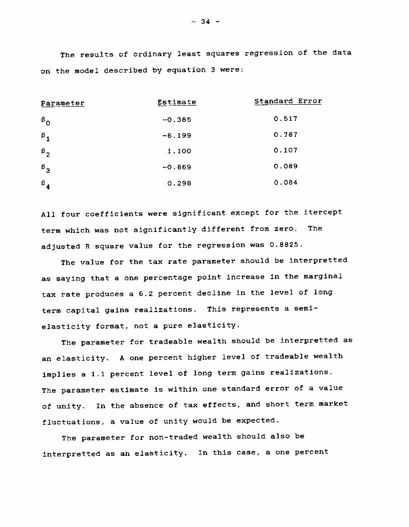
— 34 —

The results of ordinary least squares regression of the data

on the model described by equation 3 were:

Parameter Estimate Standard Error

—0.385 0.517

—6.199 0.787

a2 1.100 0.107

—0.869 0.089

1340.298 0.084

All four coefficients were significant except for the itercept

term which was not significantly different from zero. The

adjusted R square value for the regression was 0.8825.

The value for the tax rate parameter should be interpretted

as saying that a one percentage point increase in the marginal

tax rate produces a 6.2 percent decline in the level of long

term capital gains realizations. This represents a semi—

elasticity format, not a pure elasticity.

The parameter for tradeable wealth should be interpretted as

an elasticity. A one percent higher level of tradeable wealth

implies a 1.1 percent level of long term gains realizations.

The parameter estimate is within one standard error of a value

of unity. In the absence of tax effects, and short term market

fluctuations, a value of unity would be expected.

The parameter for non—traded wealth should also be

interpretted as an elasticity. In this case, a one percent

— 35 —

increase in non—traded wealth decreases net long term capital

gains realizations by 0.87 percent. A negative value on this

parameter can be understood in the context of what comprises

non-traded wealth. A substantial portion of this wealth

represents highly liquid assets such as cash, savings and

checking deposits, and government securities. If long term

capital gains realizations are designed to raise cash for

consumption purposes, we would expect to see realizations

negatively correlated with the existing level of these liquid

assets.

The final parameter value also represents an elasticity. A

one percent increase in the revaluation of traded assets in a

given year increases net capital gains realizations by 0.3

percent. This parameter suggests that increases in stock,

business, or real estate prices prompt increased realizations.

Note that this is in addition to the increase in realizations

due to a higher level of wealth. So, for example, in a year in

which there is a 20 percent rise in the value of traded assets

we could expect capital gains realizations to be higher by a

total of about 28 percent, 22 percent due to the higher level of

wealth and 6 percent due to the price increases in that year.

If prices remained stable in later years, capital gains

realizations would fall 6 percent in the following year to

maintain a new, permanent level of gains 22 percent higher than

the initial level.

Before exploring the robustness of these results, consider

an additional interpretation for the tax rate parameter. In

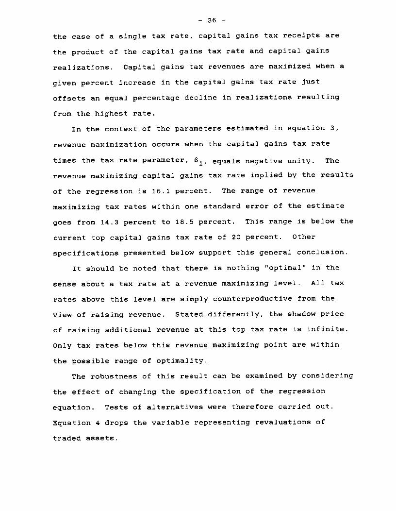
— 36 —

the case of a single tax rate, capital gains tax receipts are

the product of the capital gains tax rate and capital gains

realizations. Capital gains tax revenues are maximized when a

given percent increase in the capital gains tax rate just

offsets an equal percentage decline in realizations resulting

from the highest rate.

In the context of the parameters estimated in equation 3,

revenue maximization occurs when the capital gains tax rate

times the tax rate parameter, 31, equals negative unity. The

revenue maximizing capital gains tax rate implied by the results

of the regression is 16.1 percent. The range of revenue

maximizing tax rates within one standard error of the estimate

goes from 14.3 percent to 18.5 percent. This range is below the

current top capital gains tax rate of 20 percent. Other

specifications presented below support this general conclusion.

It should be noted that there is nothing "optimal" in the

sense about a tax rate at a revenue maximizing level. All tax

rates above this level are simply counterproductive from the

view of raising revenue. Stated differently, the shadow price

of raising additional revenue at this top tax rate is infinite.

Only tax rates below this revenue maximizing point are within

the possible range of optimality.

The robustness of this result can be examined by considering

the effect of changing the specification of the regression

equation. Tests of alternatives were therefore carried out.

Equation 4 drops the variable representing revaluations of

traded assets.

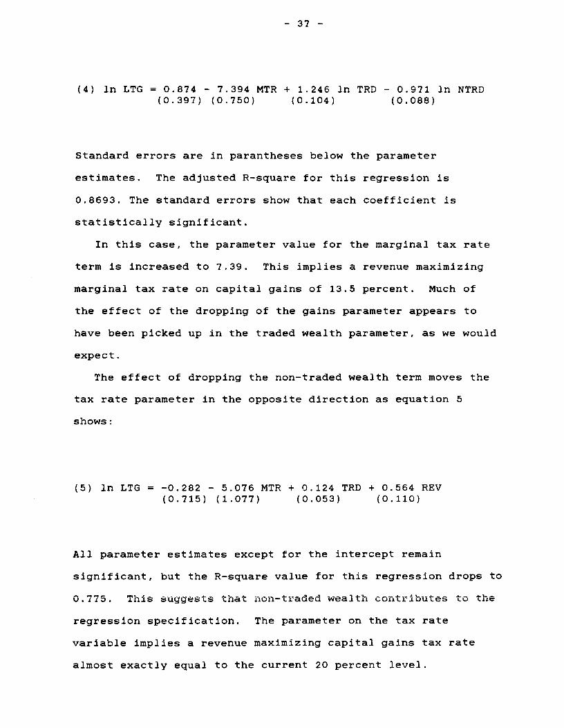
— 37 —

(4) in LTG = 0.874 - 7.394 MTR + 1.246 in TRD - 0.971 in NTRD(0.397) (0.750) (0.104) (0.088)

Standard errors are in parantheses below the parameter

estimates. The adjusted R—square for this regression is

0.8693. The standard errors show that each coefficient is

statistically significant.

In this case, the parameter value for the marginal tax rate

term is increased to 7.39. This implies a revenue maximizing

marginal tax rate on capital gains of 13.5 percent. Much of

the effect of the dropping of the gains parameter appears to

have been picked up in the traded wealth parameter, as we would

expect.

The effect of dropping the non-traded wealth term moves the

tax rate parameter in the opposite direction as equation 5

shows:

(5) ln LTG = —0.282 — 5.076 MTR + 0.124 TRD + 0.564 REV(0.715) (1.077) (0.053) (0.110)

All parameter estimates except for the intercept remain

significant, but the R—square value for this regression drops to

0.775. This suggests that non-traded wealth contributes to the

regression specification. The parameter on the tax rate

variable implies a revenue maximizing capital gains tax rate

almost exactly equal to the current 20 percent level.

— 38 —

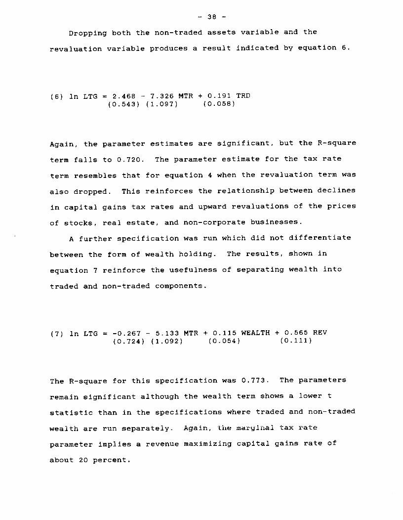
Dropping both the non-traded assets variable and the

revaluation variable produces a result indicated by equation 6.

(6) in LTG = 2.468 — 7.326 MTR + 0.191 TRD(0.543) (1.097) (0.058)

Again, the parameter estimates are significant, but the R—square

term fails to 0.720. The parameter estimate for the tax rate

term resembles that for equation 4 when the revaluation term was

also dropped. This reinforces the relationship between declines

in capital gains tax rates and upward revaluations of the prices

of stocks, real estate, and non—corporate businesses.

A further specification was run which did not differentiate

between the form of wealth holding. The results, shown in

equation 7 reinforce the usefulness of separating wealth into

traded and non—traded components.

(7) in LTG = —0.267 — 5.133 MTR + 0.115 WEALTH + 0.565 REV(0.724) (1.092) (0.054) (0.111)

The R—square for this specification was 0.773. The parameters

remain significant although the wealth term shows a lower t

statistic than in the specifications where traded and non-traded

wealth are run separately. Again, the marginal tax rate

parameter implies a revenue maximizing capital gains rate of

about 20 percent.

— 39 —

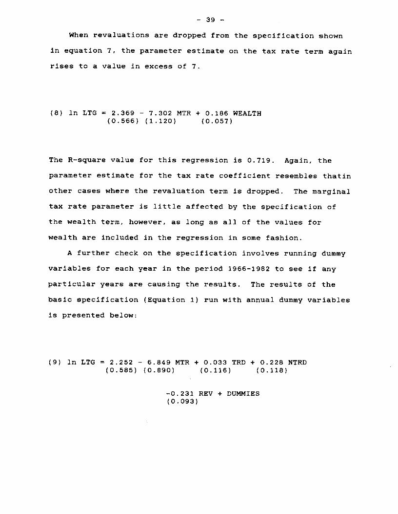
When revaluations are dropped from the specification shown

in equation 7, the parameter estimate on the tax rate term again

rises to a value in excess of 7.

(8) In LTG = 2.369 — 7.302 MTR + 0.186 WEALTH(0.566) (1.120) (0.057)

The R-square value for this regression is 0.719. Again, the

parameter estimate for the tax rate coefficient resembles thatin

other cases where the revaluation term is dropped. The marginal

tax rate parameter is little affected by the specification of

the wealth term, however, as long as all of the values for

wealth are included in the regression in some fashion.

A further check on the specification involves running dummy

variables for each year in the period 1966-1982 to see if any

particular years are causing the results. The results of the

basic specification (Equation 1) run with annual dummy variables

is presented below:

(9) In LTG = 2.252 - 6.849 MTR + 0.033 TRD + 0.228 NTRD(0.585) (0.890) (0.116) (0.118)

-0.231 REV + DUMMIES(0 .093)

— 40 —

The coefficients on the dummy variables were significant,

and illustrated an underlying time trend reflecting the rising

levels of long term gains over the period. Inclusion of these

annual data reduced the significance of the wealth and

revaluation coefficients as variations in these terms were

captured on a year—by--year basis. However, the marginal tax

rate coefficient remained highly significant, and increased in

value relative to the basic specification.

Another specification of the regression is obtained by

changing the tax rate coefficient into an elasticity format. In

this case, the natural log of the portion of the gain which the

taxpayer is allowed to keep becomes the tax parameter. This

specification presumes that a given percentage point reduction

in the tax rate, or a given percent reduction in the same value,

will have an effect which varies with the level of the tax rate.

For example, a reduction in the capital gains tax rate from

25 to 24 percent implies an increase in the share of the gain

the taxpayer keeps from 75 to 76 percent. That represents a

1.33 percent increase in the share kept by the taxpayer. The

same one percentage point reduction in tax rate from 50 to 49

would increase the taxpayer's share from 50 to 51 percent of the

gain, or by 2 percent. Similarly, a 4 percent reduction in the

tax rate, from 25 to 24, and from 50 to 48, would imply a

percent change in the after tax share far greater at the higher

tax rate (3 times as much) as at the lower tax rate.

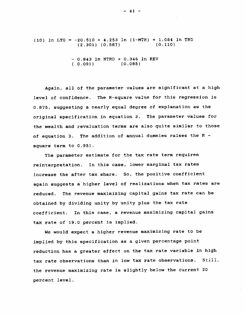
The results of such a specification are presented by

equation 10.

— 41 —

(10) in LTG = —20.510 + 4.253 in (1—MTR) ÷ 1.084 in TRD(2.301) (0.587) (0.110)

— 0.843 in NTRD + 0.346 in REV0.091) (0.085)

Again, au of the parameter vaiues are significant at a high

level of confidence. The R—square value for this regression is

0.875, suggesting a nearly equal degree of explanation as the

original specification in equation 3. The parameter values for

the wealth and revaluation terms are also quite similar to those

of equation 3. The addition of annual dummies raises the R -

square term to 0.951.

The parameter estimate for the tax rate term requires

reinterpretation. In this case, lower marginal tax rates

increase the after tax share. So, the positive coefficient

again suggests a higher level of realizations when tax rates are

reduced. The revenue maximizing capital gains tax rate can be

obtained by dividing unity by unity plus the tax rate

coefficient. In this case, a revenue maximizing capital gains

tax rate of 19.0 percent is implied.

We would expect a higher revenue maximizing rate to be

implied by this specification as a given percentage point

reduction has a greater effect on the tax rate variable in high

tax rate observations than in low tax rate observations. Still,

the revenue maximizing rate is slightly below the current 20

percent level.

— 42 —

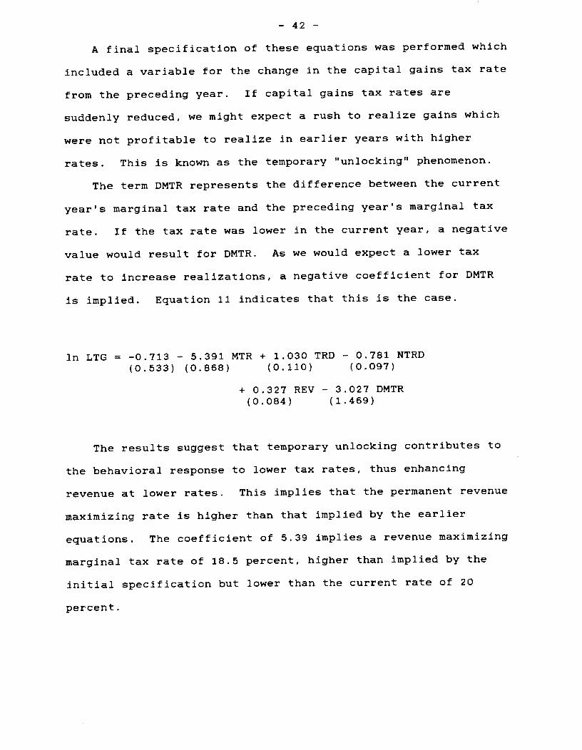
A final specification of these equations was performed which

included a variable for the change in the capital gains tax rate

from the preceding year. If capital gains tax rates are

suddenly reduced, we might expect a rush to realize gains which

were not profitable to realize in earlier years with higher

rates. This is known as the temporary "unlocking" phenomenon.

The term DMTR represents the difference between the current

year's marginal tax rate and the preceding year's marginal tax

rate. If the tax rate was lower in the current year, a negative

value would result for DMTR. As we would expect a lower tax

rate to increase realizations, a negative coefficient for DMTR

is implied. Equation 11 indicates that this is the case.

ln LTG = -0.713 — 5.391 MTR + 1.030 TRD - 0.781 NTRD

(0.533) (0.868) (0.110) (0.097)

+ 0.327 REV - 3.027 DMTR(0.084) (1.469)

The results suggest that temporary unlocking contributes to

the behavioral response to lower tax rates, thus enhancing

revenue at lower rates. This implies that the permanent revenue

maximizing rate is higher than that implied by the earlier

equations. The coefficient of 5.39 implies a revenue maximizing

marginal tax rate of 18.5 percent, higher than implied by the

initial specification but lower than the current rate of 20

percent.

— 43 —

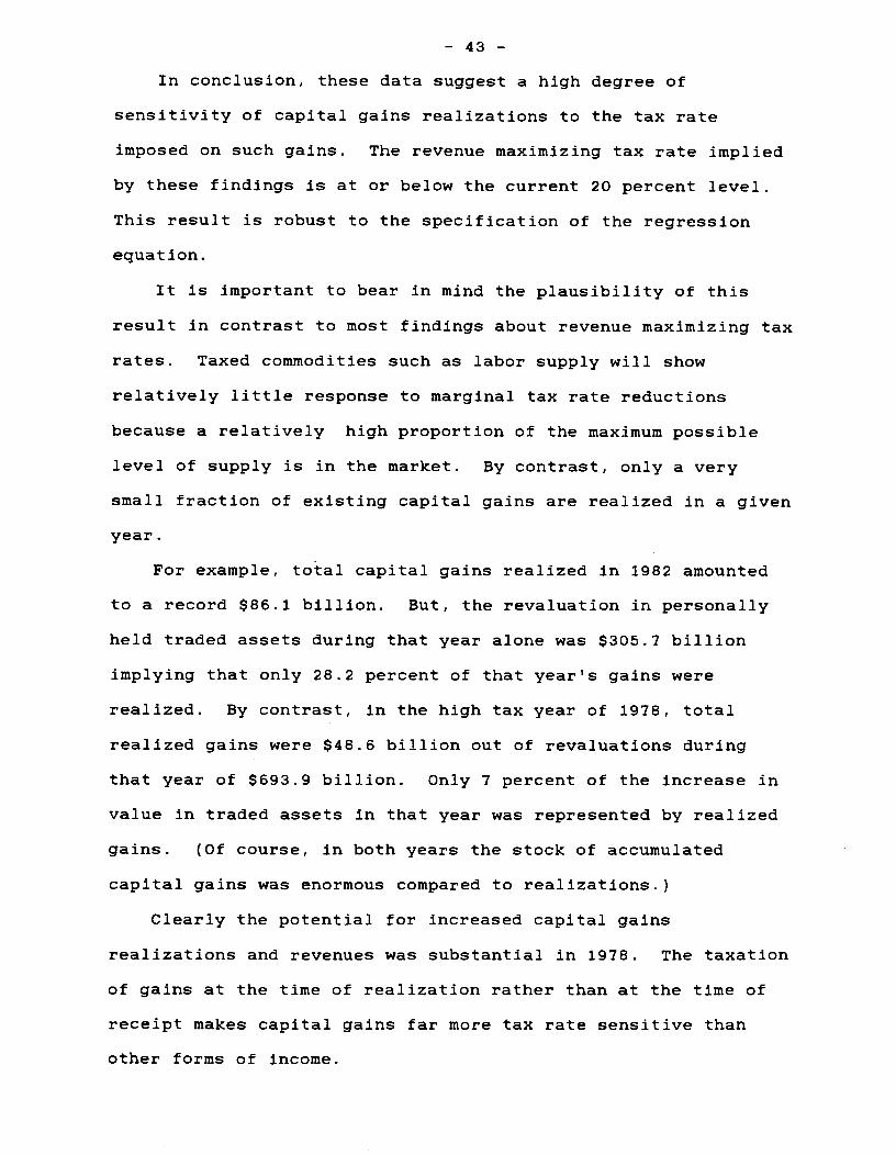
In conclusion, these data suggest a high degree of

sensitivity of capital gains realizations to the tax rate

imposed on such gains. The revenue maximizing tax rate implied

by these findings is at or below the current 20 percent level.

This result is robust to the specification of the regression

equation.

It is important to bear in mind the plausibility of this

result in contrast to most findings about revenue maximizing tax

rates. Taxed commodities such as labor supply will show

relatively little response to marginal tax rate reductions

because a relatively high proportion of the maximum possible

level of supply is in the market. By contrast, only a very

small fraction of existing capital gains are realized in a given

year.

For example, total capital gains realized in 1982 amounted

to a record $86.1 billion. But, the revaluation in personally

held traded assets during that year alone was $305.7 billion

implying that only 28.2 percent of that year's gains were

realized. By contrast, in the high tax year of 1978, total

realized gains were $48.6 billion out of revaluations during

that year of $693.9 billion. Only 7 percent of the increase in

value in traded assets in that year was represented by realized

gains. (Of course, in both years the stock of accumulated

capital gains was enormous compared to realizations.)

Clearly the potential for increased capital gains

realizations and revenues was substantial in 1978. The taxation

of gains at the time of realization rather than at the time of

receipt makes capital gains far more tax rate sensitive than

other forms of income.

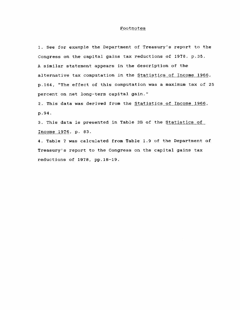
Footnotes

1. See for example the Department of Treasury's report to the

Congress on the capital gains tax reductions of 1978, p.35.

A similar statement appears in the description of the

alternative tax computation in the Statistics of Income 1966,

p.164, "The effect of this computation was a maximum tax of 25

percent on net long—term capital gain."

2. This data was derived from the Statistics of Income 1966,

p.94.

3. This data is presented in Table 3B of the Statistics of

Income 1976, p. 83.

4. Table 7 was calculated from Table 1.9 of the Department of

Treasury's report to the Congress on the capital gains tax

reductions of 1978, pp.18—i9.

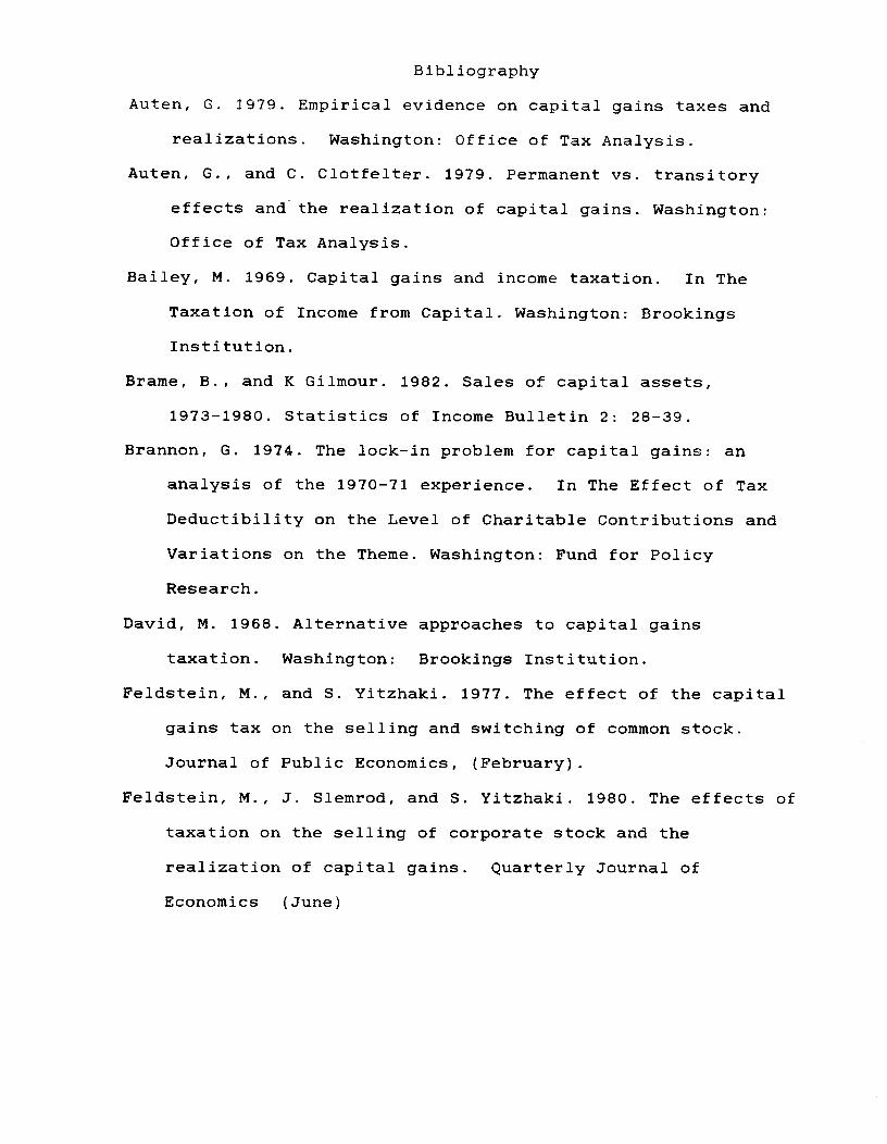
Bibliography

Auten, G. 1979. Empirical evidence on capital gains taxes and

realizations. Washington: Office of Tax Analysis.

Auten, G., and C. Clotfelter. 1979. Permanent vs. transitory

effects and the realization of capital gains. Washington:

Office of Tax Analysis.

Bailey, M. 1969. Capital gains and income taxation. In The

Taxation of Income from Capital. Washington: Brookings

Institution.

Brame, B., and K Gilmour. 1982. Sales of capital assets,

1973—1980. Statistics of Income Bulletin 2: 28—39.

Brannon, G. 1974. The lock-in problem for capital gains: an

analysis of the 1970-71 experience. In The Effect of Tax

Deductibility on the Level of Charitable Contributions and

Variations on the Theme. Washington: Fund for Policy

Research.

David, M. 1968. Alternative approaches to capital gains

taxation. Washington: Brookings Institution.

Feldstein, M., and S. Yitzhaki. 1977. The effect of the capital

gains tax on the selling and switching of common stock.

Journal of Public Economics, (February).

Feldstein, M., J. Slemrod, and S. Yitzhaki. 1980. The effects of

taxation on the selling of corporate stock and the

realization of capital gains. Quarterly Journal of

Economics (June)

Feldstein, M., J. SJ.emrod, and S. Yitzhaki. 1984. The Effects

of Taxation on the Selling of Corporate Stock and the

Realization of Capital Gains: Reply. Quarterly Journal of

EconomiCs

Fredland, E., J. Gray, and E. Sunley. 1968. The six month

holding period for capital gains: An empirical analysis of

its effect on the timing of gains. National Tax Journal

(December)

Kaplan, S. 1981. The holding period distinction of the capital

gains tax. NBER Working Paper no' 762.

King, M., and D. Fullerton. 1984. The taxation of income from

capital. Chicago: University of Chicago Press.

Lindsey, L., 1981. Is the maximum tax on earned income

effective? National Tax Journal (June)

Miller, M., and M. Scholes. 1978. Dividends and taxes. Journal

of Financial Economics 6 : 333-64.

Minarik, J. 1981. Capital Gains. In How Taxes Effect Econom.c

Behavior. Washington: Brookings Institution.

1983. Professor Feldstein on capital gains - again.

Tax Notes (May 9).

Poterba, J., 1985. How burdensome are capital gains taxes? MIT

Working Paper No. 410. (Rev. February, 1986)

Stiglitz, J. 1969. The effects of income, wealth, and capital

gains taxation on risk taking. Quarterly Journal of

Economics 83 ( ): 262—83.

United States Department of the Treasury. 1968-85. Statistics of

Income 1965-82, individual income tax returns. Washington.

1985. Capital gains tax Reductions of 1978.

Office of Tax Analysis. Washington.