A&A 598, A85 (2017)DOI: 10.1051/0004-6361/201629621c© ESO 2017

Astronomy&Astrophysics

The Tarantula Massive Binary Monitoring

II. First SB2 orbital and spectroscopic analysis for the Wolf-Rayet binary R145?

T. Shenar1, N. D. Richardson2, D. P. Sablowski3, R. Hainich1, H. Sana4, A. F. J. Moffat5, H. Todt1, W.-R. Hamann1,L. M. Oskinova1, A. Sander1, F. Tramper6, N. Langer7, A. Z. Bonanos8, S. E. de Mink9, G. Gräfener10,

P. A. Crowther11, J. S. Vink10, L. A. Almeida12, 13, A. de Koter4, 9, R. Barbá14, A. Herrero15, and K. Ulaczyk16

1 Institut für Physik und Astronomie, Universität Potsdam, Karl-Liebknecht-Str. 24/25, 14476 Potsdam, Germanye-mail: shtomer@astro.physik.uni-potsdam.de

2 Ritter Observatory, Department of Physics and Astronomy, The University of Toledo, Toledo, OH 43606-3390, USA3 Leibniz-Institut für Astrophysik Potsdam, An der Sternwarte 16, 14482 Potsdam, Germany4 Institute of Astrophysics, KU Leuven, Celestijnenlaan 200 D, 3001 Leuven, Belgium5 Département de physique and Centre de Recherche en Astrophysique du Québec (CRAQ), Université de Montréal, CP 6128,

Succ. Centre-Ville, Montréal, Québec, H3C 3J7, Canada6 European Space Astronomy Centre (ESA/ESAC), PO Box 78, 28691 Villanueva de la Cañada, Madrid, Spain7 Argelander-Institut für Astronomie der Universität Bonn, Auf dem Hügel 71, 53121 Bonn, Germany8 IAASARS, National Observatory of Athens, 15236 Penteli, Greece9 Anton Pannenkoek Astronomical Institute, University of Amsterdam, 1090 GE Amsterdam, The Netherlands

10 Armagh Observatory, College Hill, Armagh, BT61 9DG, UK11 Department of Physics and Astronomy, University of Sheffield, Sheffield S3 7RH, UK12 Instituto de Astronomia, Geofísica e Ciências, Rua do Matão 1226, Cidade Universitária São Paulo, SP, Brasil13 Dep. of Physics & Astronomy, Johns Hopkins University, Bloomberg Center for Physics and Astronomy, 3400N Charles St, USA14 Departamento de Física y Astronomía, Universidad de la Serena, Av. Juan Cisternas 1200 Norte, La Serena, Chile15 Instituto de Astrofísica, Universidad de La Laguna, Avda. Astrofísico Francisco Sánchez s/n, 38071 La Laguna, Tenerife, Spain16 Warsaw University Observatory, Al. Ujazdowskie 4, 00-478 Warszawa, Poland

Received 30 August 2016 / Accepted 20 October 2016

ABSTRACT

We present the first SB2 orbital solution and disentanglement of the massive Wolf-Rayet binary R145 (P = 159 d) located in theLarge Magellanic Cloud. The primary was claimed to have a stellar mass greater than 300 M, making it a candidate for beingthe most massive star known to date. While the primary is a known late-type, H-rich Wolf-Rayet star (WN6h), the secondary hasso far not been unambiguously detected. Using moderate-resolution spectra, we are able to derive accurate radial velocities forboth components. By performing simultaneous orbital and polarimetric analyses, we derive the complete set of orbital parameters,including the inclination. The spectra are disentangled and spectroscopically analyzed, and an analysis of the wind-wind collision zoneis conducted. The disentangled spectra and our models are consistent with a WN6h type for the primary and suggest that the secondaryis an O3.5 If*/WN7 type star. We derive a high eccentricity of e = 0.78 and minimum masses of M1 sin3 i ≈ M2 sin3 i = 13 ± 2 M,with q = M2/M1 = 1.01 ± 0.07. An analysis of emission excess stemming from a wind-wind collision yields an inclination similar tothat obtained from polarimetry (i = 39 ± 6). Our analysis thus implies M1 = 53+40

−20 and M2 = 54+40−20 M, excluding M1 > 300 M. A

detailed comparison with evolution tracks calculated for single and binary stars together with the high eccentricity suggests that thecomponents of the system underwent quasi-homogeneous evolution and avoided mass-transfer. This scenario would suggest currentmasses of ≈80 M and initial masses of Mi,1 ≈ 105 and Mi,2 ≈ 90 M, consistent with the upper limits of our derived orbital masses,and would imply an age of ≈2.2 Myr.

Key words. binaries: spectroscopic – stars: Wolf-Rayet – stars: massive – Magellanic Clouds – stars: individual: R 145 –stars: atmospheres

1. Introduction

Ever-growing efforts are made to discover the most massivestars in the Universe (e.g., Massey & Hunter 1998; Schnurr et al.2008a; Bonanos 2009; Bestenlehner et al. 2011; Tramper et al.2016). Because of their extreme influence on their environment,understanding the formation, evolution, and death of massive

? A copy of the disentangled spectra, as either FITS files or tablesare available at the CDS via anonymous ftp tocdsarc.u-strasbg.fr (130.79.128.5) or viahttp://cdsarc.u-strasbg.fr/viz-bin/qcat?J/A+A/598/A85

stars is imperative for a multitude of astrophysical fields. Estab-lishing the upper mass limit for stars is one of the holy grails ofstellar physics, laying sharp constraints on the initial mass func-tion (Salpeter 1955; Kroupa 2001) and massive star formation(Bonnell et al. 1997; Oskinova et al. 2013). Current estimatesfor an upper mass limit range from ≈120 M (e.g., Oey & Clarke2005) to &300 M (e.g., Crowther et al. 2010; Schneider et al.2014a; Vink 2015).

However, the only reliable method to weigh stars is by ana-lyzing the orbits of stars in binaries (Andersen 1991; Torres et al.2010). This is especially crucial for massive Wolf-Rayet (WR)

Article published by EDP Sciences A85, page 1 of 16

A&A 598, A85 (2017)

R145 R136

Fig. 1. Sky area around R145 (credit: NASA, ESA, E. Sabbi, STScI).The image was obtained using the Hubble Space Telescope’s (HST)WFC3 and ACS cameras in filters that roughly overlap with the I, J,and H bands. The image size is ≈2.5′ × 1.7′. North is up and east tothe left. The arrows indicate the positions of R145 and the star clusterR 136. The distance between R145 and R 136 is ≈1.3′, or in projection,≈19 pc.

stars, whose powerful winds make it virtually impossible to es-timate their surface gravities. Fortunately, massive stars (M &8 M) tend to exist in binary or multiple systems (Mason et al.2009; Maíz Apellániz 2010; Oudmaijer & Parr 2010; Sana et al.2012, 2014; Sota et al. 2014; Aldoretta et al. 2015).

Primarily as a result of mass-transfer, the evolutionary pathof a star in a binary can greatly deviate from that of an identicalstar in isolation (Paczynski 1973; Langer 2012; de Mink et al.2014). The impact and high frequency of binarity make binariesboth indispensable laboratories for the study of massive stars andimportant components of stellar evolution. Hence, it is impera-tive to discover and study massive binary systems in the Galaxyand the Local Group.

R145 (BAT99 119, HDE 269928, Brey 90, VFTS 695) isa known massive binary situated in the famous Tarantula neb-ula in the Large Magellanic Cloud (LMC), about 19 pc awayfrom the massive cluster R 136 in projection (see Fig. 1). Thesystem’s composite spectrum was classified WN6h in the origi-nal BAT99 catalog (Breysacher et al. 1999), which, according tothis and past studies (e.g., Schnurr et al. 2009, S2009 hereafter),corresponds to the primary. The primary thus belongs to the classof late WR stars that have not yet exhausted their hydrogen con-tent, and core H-burning is most likely still ongoing.

The system was speculated to host some of the most mas-sive and luminous stars in the Local Group. Erroneously assum-ing a circular orbit, Moffat (1989) detected a periodic Dopplershift with a period of P = 25.17 d, concluding R145 to be anSB1 binary. A significantly different period of 158.8 ± 0.1 dwas later reported by S009, who combined data from Moffat(1989) with their own and found a highly eccentric system.S009 could not derive a radial velocity (RV) curve for the sec-ondary. However, they attempted to estimate the secondary’sRV amplitude by looking for “resonance” velocity amplitudesthat would strengthen the secondary’s features in a spectrumformed by coadding the spectra in the secondary’s frame of ref-erence, under the assumption that the secondary is mainly anabsorption-line star moving in antiphase to the primary star.Combined with the orbital inclination of i = 38 ± 9 thatthey derived, their results tentatively implied that the systemcomprises two incredibly massive stars of ≈300 and ≈125 M,

making it potentially the most massive binary system knownto date. For comparison, binary components of similar spec-tral type typically have masses ranging from ≈50 to ≈100 M(e.g., WR 22, Rauw et al. 1996; WR 20a, Bonanos et al. 2004;Rauw et al. 2004; WR 21a, Niemela et al. 2008; Tramper et al.2016; HD 5980, Koenigsberger et al. 2014; NGC 3603-A1,Schnurr et al. 2008a); masses in excess of 300 M were so faronly reported for putatively single stars (e.g., Crowther et al.2010) based on comparison with evolutionary models.

With such high masses, signatures for wind-wind collisions(WWC) are to be expected (Moffat 1998). WWC excess emis-sion can be seen photometrically as well as spectroscopically,and can thus also introduce a bias when deriving RVs. WWCsignatures do not only reveal information on the dynamics andkinematics of the winds, but can also constrain the orbital in-clination, which is crucial for an accurate determination of thestellar masses. Polarimetry offers a further independent tool toconstrain orbital inclinations of binary systems (Brown et al.1978). Both approaches are used in this study to constrain theorbital inclination i. For high inclination angles, photometricvariability that is due to photospheric or wind eclipses can alsobe used to constrain i (e.g., Lamontagne et al. 1996). At thelow inclination angle of R145 (see Sects. 4 and 7, as well asS2009), however, eclipses are not expected to yield significantconstraints.

Using 110 high-quality Fibre Large Array Multi ElementSpectrograph (FLAMES) spectra (Sect. 2), we are able to derivefor the first time a double-lined spectroscopic orbit for R145. Weidentify lines that enable us to construct a reliable SB2 RV curve(Sect. 3). The majority of the spectra were taken as part of theVLT FLAMES-Tarantula survey (VFTS, Evans et al. 2011) andfollow-up observations (PI: H. Sana). The study is conductedin the framework of the Tarantula Massive Binary Monitoring(TMBM) project (Almeida et al. 2017, Paper I hereafter).

The RVs of both components are fitted simultaneously withpolarimetric data to obtain accurate orbital parameters (Sect. 4).In Sect. 5, we disentangle the spectrum into its constituent spec-tra. Using the disentangled spectra, an X-shooter spectrum,and additional observational material, we perform a multiwave-length spectroscopic analysis of the system using the PotsdamWolf-Rayet (PoWR) model atmosphere code to derive the fun-damental stellar parameters and abundances of the two stars(Sect. 6). An analysis of WWC signatures is presented in Sect. 7.A discussion of the evolutionary status of the system in light ofour results is presented in Sect. 8. We conclude with a summaryin Sect. 9.

2. Observational data

The FLAMES spectra (072.C-0348, Rubio; 182.D-0222, Evans;090.D-0323, Sana; 092.D-0136, Sana) were secured between2004 and 2014 with the FLAMES instrument mounted on theVery Large Telescope (VLT), Chile, partly in the course oftwo programs: the VLT FLAMES Tarantula Survey (Evans et al.2011), and the TMBM project. They cover the spectral range3960–4560 Å, have a typical signal-to-noise ratio (S/N) of 100,and a resolving power of R ≈ 8000 (see Paper I for more in-formation). The spectra were rectified using an automated rou-tine that fits a piecewise first-order polynomial to the apparentcontinuum and cleaned from cosmic events using a dedicatedPython routine we developed.

For the spectral analysis, we use an X-shooter (Vernet et al.2011) spectrum (085.D-0704, PI: Sana) taken on 22 April 2010(φ ≈ 0.5, i.e., apastron, with the phase calculated using the

A85, page 2 of 16

T. Shenar et al.: A first SB2 orbital and spectroscopic analysis for the Wolf-Rayet binary R145

Table 1. Derived orbital parameters.

Parameter Value

Porb [days] 158.760T0 [MJD] 56 022.6 ± 0.2K1 [km s−1 ] 96 ± 3K2 [km s−1 ] 95 ± 4e 0.788 ± 0.007ω[] 61 ± 7Morb,1 sin3 i [M] 13.2 ± 1.9Morb,2 sin3 i [M] 13.4 ± 1.9a1 sin i [R] 302 ± 10a2 sin i [R] 299 ± 10V0 [km s−1 ] 270 ± 5Ω [] 62 ± 7i [] 39 ± 6τ∗ 0.10 ± 0.01Q0 −2.13 ± 0.02U0 0.58 ± 0.02γ 0.87 ± 0.07Morb,1 [M] 53+40

−20

Morb,2 [M] 54+40−20

a1 [R] 480+90−65

a2 [R] 475+100−70

Notes. Derived orbital parameters from a simultaneous fit of theFLAMES RVs and the polarimetry. The period is fixed to the valuefound from the SB1 fitting using all published RVs for the primary (seeSect. 3)

He

II 1

3-4

NIV

He

II 1

2-4

Hδ

He

II 1

1-4

He

II 1

0-4

Hγ

He

I

He

I

He

II 9

-4

NV

4-3

NII

I

He

II 4

-3

He

II 8

-4

Hβ

NV

7-6

He

II 7

-4

CIV

He

I

Na

I i.

s.

He

II 1

5-5

Hα

He

II 6

-4

He

II 1

3-5

1

2

3

4

5

4000 4500 5000 5500 6000 6500

λ / Ao

No

rm

ali

zed

flu

x

Fig. 2. Segment of the X-shooter spectrum of R145.

ephemeris given in Table 1 in Sect. 4). The spectrum covers therange 3000–25 000 Å. It has an S/N ≈ 100 and a resolvingpower of R ≈ 7500 in the spectral range 5500–10 000 Å andR ≈ 5000 in the ranges 3000–5500 Å and 10 000–25 000 Å. Itwas rectified by fitting a first-order polynomial to the apparentcontinuum. A segment of the spectrum is shown in Fig. 2.

We make use of two high-resolution (HIRES), flux-calibrated International Ultraviolet Explorer (IUE) spectra avail-able in the IUE archive. The two spectra (swp47847, PM048, PI:Bomans; swp47836, PM033, PI: de Boer) were obtained on 08

He

II /

Hε

He

II 1

3-4

NIV

SiI

VH

eII

12-

4H

δN

III

SiI

V

He

II 1

1-4

He

II 1

0-4

Hγ

He

I

He

I

NII

I, I

V

He

II 9

-4

1.0

1.5

4000 4100 4200 4300 4400 4500

λ / Ao

No

rmali

zed

flu

x

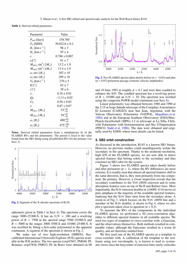
Fig. 3. Two FLAMES spectra taken shortly before (φ = −0.03) and after(φ = 0.07) periastron passage (extreme velocity amplitudes).

and 10 June 1993 at roughly φ = 0.7 and were thus coadded toenhance the S/N. The coadded spectrum has a resolving powerof R ≈ 10 000 and an S/N ≈ 10. The spectrum was rectifiedusing the composite PoWR model continuum (see Sect. 6).

Linear polarimetry was obtained between 1988 and 1990 atthe 2.15 m Jorge Sahade telescope of the Complejo AstronómicoEl Leoncito (CASLEO) near San Juan, Argentina, with theVatican Observatory Polarimeter (VATPOL, Magalhaes et al.1984) and at the European Southern Observatory (ESO)/Max-Planck-Gesellschaft (MPG) 2.2 m telescope at La Silla, Chile,with Polarimeter with Instrumentation and Sky COmpensation(PISCO, Stahl et al. 1986). The data were obtained and origi-nally used by S2009, where more details can be found.

3. SB2 orbit constructionAs discussed in the introduction, R145 is a known SB1 binary.However, no previous studies could unambiguously isolate thesecondary in the spectrum. Thanks to the moderate-resolution,high S/N of the FLAMES spectra, we are now able to detectspectral features that belong solely to the secondary and thusconstruct an SB2 orbit for the system.

Figure 3 shows two FLAMES spectra taken shortly beforeand after periastron (φ = 1), where the RV differences are mostextreme. It is readily seen that almost all spectral features shift inthe same direction, that is, they stem primarily from one compo-nent, the primary. However, a closer inspection reveals that thesecondary contributes to the N iv λ4058 emission and to someabsorption features seen on top of He II and Balmer lines. Mostimportantly, the Si iv emission doublet at λλ4089, 4116 moves inpure antiphase to the majority of the available spectral features,implying that the Si iv lines stem from the secondary alone. Azoom-in of Fig. 3, which focuses on the N iv λ4058 line and amember of the Si iv doublet, is shown in Fig. 4, where we alsoplot a spectrum taken close to apastron (φ ≈ 0.5).

To measure the RVs of the components in the individualFLAMES spectra, we performed a 1D cross-correlation algo-rithm to different spectral features in all available spectra. Wetried two types of templates to cross-correlate with: a Gaussian,and the observations themselves. Both methods resulted in com-parable values, although the Gaussians resulted in a worse fitquality, and are therefore omitted here.

We first used one of the FLAMES spectra as a template tocross-correlate with. A calibration of the template to the rest-frame using rest wavelengths λ0 is known to lead to system-atic errors since the barycenter of emission lines rarely coincides

A85, page 3 of 16

A&A 598, A85 (2017)

NIV

Si

IV

1.0

1.5

4040 4060 4080

λ / Ao

No

rm

ali

zed

flu

x

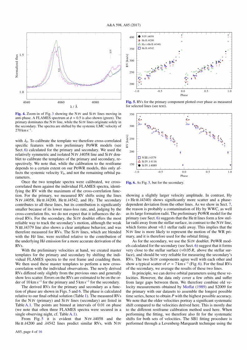
Fig. 4. Zoom-in of Fig. 3 showing the N iv and Si iv lines moving inanti-phase. A FLAMES spectrum at φ ≈ 0.5 is also shown (green). Theprimary dominates the N iv line, while the Si iv lines originate solely inthe secondary. The spectra are shifted by the systemic LMC velocity of270 km s−1.

with λ0. To calibrate the template we therefore cross-correlatedspecific features with two preliminary PoWR models (seeSect. 6) calculated for the primary and secondary. We used therelatively symmetric and isolated N iv λ4058 line and Si iv dou-blet to calibrate the templates of the primary and secondary, re-spectively. We note that, while the calibration to the restframedepends to a certain extent on our PoWR models, this only af-fects the systemic velocity V0, and not the remaining orbital pa-rameters.

Once the two template spectra were calibrated, we cross-correlated them against the individual FLAMES spectra, identi-fying the RV with the maximum of the cross-correlation func-tion. For the primary, we measured RV shifts using the linesN iv λ4058, He ii λ4200, He ii λ4542, and Hγ. The secondarycontributes to all these lines, but its contribution is significantlysmaller because of its lower mass-loss rate, and, judging by thecross-correlation fits, we do not expect that it influences the de-rived RVs. For the secondary, the Si iv doublet offers the mostreliable way to track the secondary’s motion, although the weakN iii λ4379 line also shows a clear antiphase behavior, and wastherefore measured for RVs. The Si iv lines, which are blendedwith the Hδ line, were rectified relative to the contribution ofthe underlying Hδ emission for a more accurate derivation of theRVs.

With the preliminary velocities at hand, we created mastertemplates for the primary and secondary by shifting the indi-vidual FLAMES spectra to the rest frame and coadding them.We then used these master templates to perform a new cross-correlation with the individual observations. The newly derivedRVs differed only slightly from the previous ones and generallyshow less scatter. Errors on the RVs are estimated to be on the or-der of 10 km s−1 for the primary and 5 km s−1 for the secondary.

The derived RVs for the primary and secondary as a func-tion of phase are shown in Figs. 5 and 6. The phase is calculatedrelative to our final orbital solution (Table 1). The measured RVsfor the N iv (primary) and Si iv lines (secondary) are listed inTable A.1. The points are binned at intervals of 0.01 on phase(we note that often three FLAMES spectra were secured in asingle observing night, cf. Table A.1).

From Fig. 5 it is evident that N iv λ4058 and theHe ii λ4200 and λ4542 lines predict similar RVs, with N iv

N IV λ4058

He II λ4200

Hγ (+He II λ4340)

He II λ4542

200

250

300

350

400

-1.0 -0.5 0.0 0.5 1.0

Phase

RV

[km

/s]

Fig. 5. RVs for the primary component plotted over phase as measuredfor selected lines (see text).

Si IV λ 4089Si IV λ 4116N III λ 4379

150

200

250

300

350

-1.0 -0.5 0.0 0.5 1.0

Phase

RV

[km

/s]

Fig. 6. As Fig. 5, but for the secondary.

showing a slightly larger velocity amplitude. In contrast, Hγ(+ He ii λ4340) shows significantly more scatter and a phase-dependent deviation from the other lines. As we show in Sect. 7,the reason is probably a contamination of Hγ by WWC, as wellas its large formation radii. The preliminary PoWR model for theprimary (see Sect. 6) suggests that the He ii lines form a few stel-lar radii away from the stellar surface, in contrast to the N iv line,which forms about ≈0.1 stellar radii away. This implies that theN iv line is more likely to represent the motion of the WR pri-mary, and it is therefore used for the orbital fitting.

As for the secondary, we use the Si iv doublet. PoWR mod-els calculated for the secondary (see Sect. 6) suggest that it formsvery close to the stellar surface (≈0.05 R∗ above the stellar sur-face), and should be very reliable for measuring the secondary’sRVs. The two Si iv components agree well with each other andshow a typical scatter of σ ≈ 7 km s−1 (Fig. 6). For the final RVsof the secondary, we average the results of these two lines.

In principle, we can derive orbital parameters using these ve-locities. However, the data only cover a few orbits and sufferfrom large gaps between them. We therefore combine old ve-locity measurements obtained by Moffat (1989) and S2009 forthe primary with our datasets to assemble the longest possibletime series, hence to obtain P with the highest possible accuracy.We note that the older velocities portray a significant systematicshift compared to the velocities derived here. This is mostly dueto the different restframe calibration method used here. Whenperforming the fitting, we therefore also fit for the systematicshifts for both sets of velocities. The SB1 fitting procedure isperformed through a Levenberg-Marquardt technique using the

A85, page 4 of 16

T. Shenar et al.: A first SB2 orbital and spectroscopic analysis for the Wolf-Rayet binary R145

results of a Fourier analysis as a guess value for the initial period(Gosset et al. 2001).

From the SB1 fit, we derive the period Porb = 158.760 ±0.017 d, the epoch of periastron passage T0[MJD] = 56 022.4 ±0.8, the RV amplitude of the primary K1 = 78 ± 3 km s−1, theeccentricity e = 0.75± 0.01, and the argument of periastron ω =61±1. Since the older velocities suffer from significantly largererrors, we do not adopt all orbital parameters derived, but onlythe period, which benefits significantly from the ≈30 yr of cov-erage. We do not find evidence for apsidal motion in the system,which may, however, be a consequence of the fact that the newdata are of much higher quality than previous ones. In the nextsection, we analyze the polarimetric data simultaneously withthe FLAMES data to better determine the orbital parameters andthe orbital inclination. We note that the assumption here is thatthe period change caused by mass-loss from the system is neg-ligible during these 30 yr. Since roughly 10−4.3 M are lost fromthe system each year (see Sect. 6), approx. ∆Mtot = 0.001 Mwere lost within 30 yr. The period change within 30 yr canbe estimated through Pi/Pf =

(Mtot,f/Mtot,i

)2 (Vanbeveren et al.1998). Assuming Mtot = 100 M for an order-of-magnitude es-timate, we obtain a difference in the period that is smaller thanour error, and thus negligible.

4. Simultaneous polarimetry and RV fitting

Fitting the polarimetric data simultaneously with the RV data en-ables us to lay tighter constraints on the orbital parameters. Fur-thermore, as opposed to an RV analysis, polarimetry can yieldconstraints on the inclination i. As the orbital masses scale asMorb ∝ sin3 i, knowing i is crucial.

The polarimetric analysis is based on ideas developed byBrown et al. (1978, 1982), later corrected by Simmons & Boyle(1984). A similar analysis for the system was performed byS2009. As such, light emitted from a spherically symmetric staris unpolarized. While Thomson scattering off free electrons inthe stellar wind causes the photons to be partially linearly polar-ized, the total polarization measured in the starlight cancels outif its wind is spherically symmetric. However, when the light ofa star is scattered in the wind of its binary companion, the sym-metry is broken, and some degree of polarization is expected.The degree of polarization depends on the amount and geometryof the scattering medium, which depends on the properties of thewind (e.g., mass-loss) and on the orbital phase.

In our case, the dominant source of free electrons wouldclearly be the wind of the primary WR star (see also Sect. 6),although some of the primary’s light may also be scattered in thewind of the secondary star. We first assume that only the wind ofthe primary contributes to the polarization, given its dominanceover that of the secondary. We will later relax this assumption.Following Robert et al. (1992), the Stokes parameters U(φ) andQ(φ) can be written as the sum of the (constant) interstellar po-larizations U0, Q0 and phase-dependent terms:

U(φ) = U0 + ∆Q(φ) sin Ω + ∆U(φ) cos Ω

Q(φ) = Q0 + ∆Q(φ) cos Ω − ∆U(φ) sin Ω, (1)

where Ω is the position angle of the ascending node, and ∆Q(φ),∆U(φ) (in the case of spherically symmetric winds) are given by

∆U(φ) = −2τ3(φ) cos i sin(2λ(φ))

∆Q(φ) = −τ3(φ)[(

1 + cos2 i)

cos(2λ(φ)) − sin2 i]. (2)

150

200

250

300

350

400

450

-0.5 0.0 0.5 1.0

φ

RV

[k

m/s

]

Fig. 7. Orbital solution plotted against the measured RVs for theN iv λ4058 line (primary, black stars) and the averaged velocities of theSi iv λλ4089, 4116 doublet (secondary, green triangles).

Here, λ(φ) = ν(φ) + ω − π/2 is the longitude of the scatteringsource (primary) with respect to the illuminating source (sec-ondary). ν is the true anomaly, ω is the argument of periastron.τ3 is the effective optical depth of the scatterers (see Eqs. (4) and(5) in Robert et al. 1992) which scales with the (constant) to-tal optical depth τ∗ of the primary star (see Moffat et al. 1998).St.-Louis et al. (1988) assumed that τ3(φ) = τ∗ (a/D(φ))γ, whereD(φ) is the separation between the companions, and γ is a num-ber on the order of unity. Brown et al. (1982) showed that γ ≈ 2in the case of a wind that is localized closely to the primary’sstellar surface. However, this need not be the case for WR stars.

The free parameters involved in the polarimetry fitting aretherefore Ω, i, τ∗,Q0,U0, and γ, as well as the orbital parame-ters P, ω, and e. This model can easily be generalized if bothcompanions possess winds that can significantly contribute tothe total polarization. In this case, τ∗ is the sum of the opticaldepths of both stars, weighted with the relative light ratios (seeEq. (2) in Brown et al. 1982). The formalism may therefore beimplemented here, with the only consequence that τ∗ relates tothe mass-loss rates of the two companions.

The simultaneous fitting of the FLAMES RVs and the polari-metric data is performed through a χ2 minimization algorithm,with a relative weight given to the RV and polarimetric data cho-sen so that both types of data have a similar contribution to thetotal χ2. Best-fit RV and Q/U curves are shown in Figs. 7 and8. During the fitting procedure, the period is fixed to the valueinferred from the combined RV sample (see Sect. 3). The corre-sponding best-fitting parameters are given in Table 1.

The inclination found in this study is very similar to that re-ported by S2009, which is not surprising given that we make useof the same polarimetric data. We note that clumps in the windcan generally enhance the scattering and may therefore lead toan overestimation of the inclination. The eccentricity is found tobe hihger, e = 0.788±0.007 as opposed to e = 0.70±0.01 foundby S2009. This also affects the remaining orbital parameters (cf.Table 5 in S2009). Most importantly, the orbital masses foundhere are much lower, ≈55+40

−20 M for each component comparedto M1 & 300 and M2 & 125 that were inferred by S2009. Thereason for this discrepancy is the improved derivation of K2 inour study. While we cannot supply a definitive reason for the er-roneous derivation of K2 by S2009, we suggest that it may berelated to the fact that the secondary exhibits emission features

A85, page 5 of 16

A&A 598, A85 (2017)

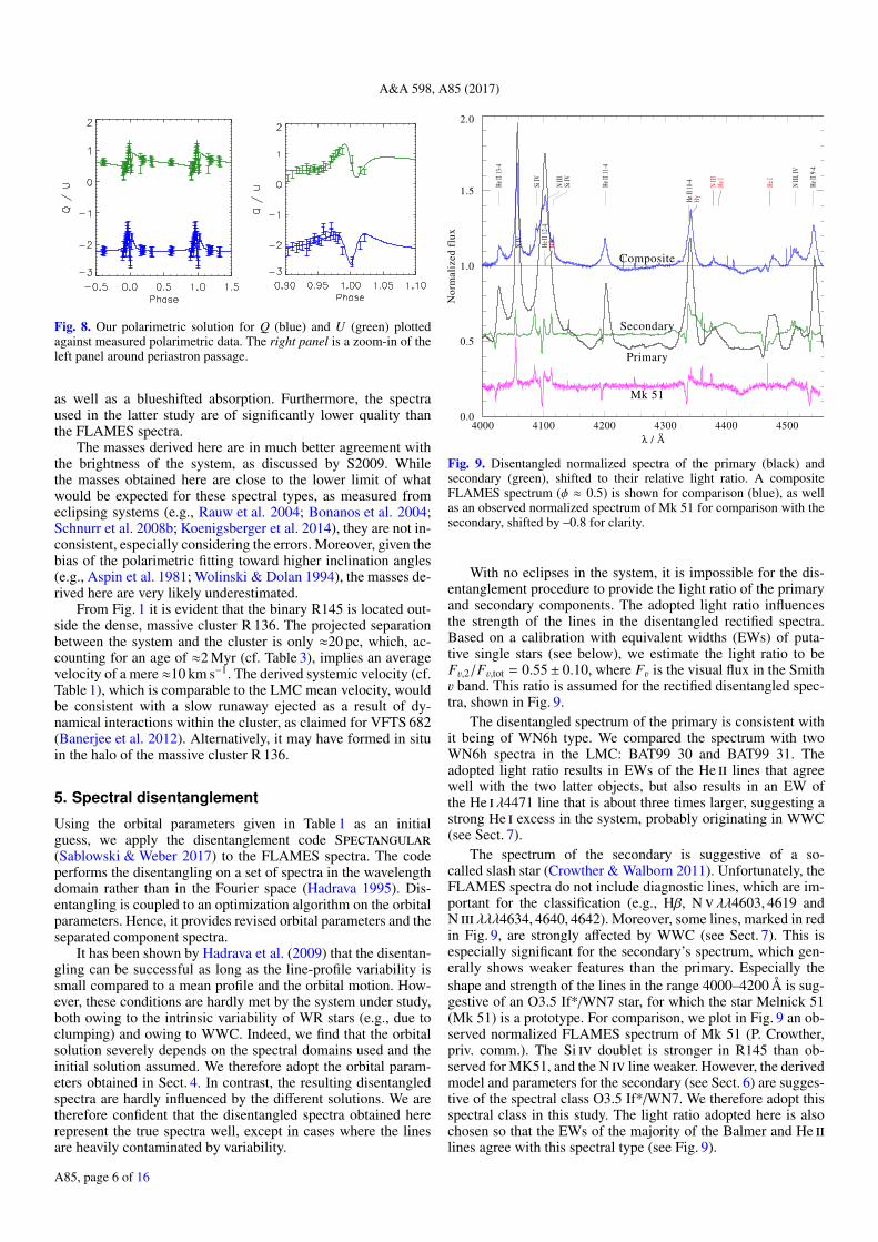
Fig. 8. Our polarimetric solution for Q (blue) and U (green) plottedagainst measured polarimetric data. The right panel is a zoom-in of theleft panel around periastron passage.

as well as a blueshifted absorption. Furthermore, the spectraused in the latter study are of significantly lower quality thanthe FLAMES spectra.

The masses derived here are in much better agreement withthe brightness of the system, as discussed by S2009. Whilethe masses obtained here are close to the lower limit of whatwould be expected for these spectral types, as measured fromeclipsing systems (e.g., Rauw et al. 2004; Bonanos et al. 2004;Schnurr et al. 2008b; Koenigsberger et al. 2014), they are not in-consistent, especially considering the errors. Moreover, given thebias of the polarimetric fitting toward higher inclination angles(e.g., Aspin et al. 1981; Wolinski & Dolan 1994), the masses de-rived here are very likely underestimated.

From Fig. 1 it is evident that the binary R145 is located out-side the dense, massive cluster R 136. The projected separationbetween the system and the cluster is only ≈20 pc, which, ac-counting for an age of ≈2 Myr (cf. Table 3), implies an averagevelocity of a mere ≈10 km s−1. The derived systemic velocity (cf.Table 1), which is comparable to the LMC mean velocity, wouldbe consistent with a slow runaway ejected as a result of dy-namical interactions within the cluster, as claimed for VFTS 682(Banerjee et al. 2012). Alternatively, it may have formed in situin the halo of the massive cluster R 136.

5. Spectral disentanglement

Using the orbital parameters given in Table 1 as an initialguess, we apply the disentanglement code Spectangular(Sablowski & Weber 2017) to the FLAMES spectra. The codeperforms the disentangling on a set of spectra in the wavelengthdomain rather than in the Fourier space (Hadrava 1995). Dis-entangling is coupled to an optimization algorithm on the orbitalparameters. Hence, it provides revised orbital parameters and theseparated component spectra.

It has been shown by Hadrava et al. (2009) that the disentan-gling can be successful as long as the line-profile variability issmall compared to a mean profile and the orbital motion. How-ever, these conditions are hardly met by the system under study,both owing to the intrinsic variability of WR stars (e.g., due toclumping) and owing to WWC. Indeed, we find that the orbitalsolution severely depends on the spectral domains used and theinitial solution assumed. We therefore adopt the orbital param-eters obtained in Sect. 4. In contrast, the resulting disentangledspectra are hardly influenced by the different solutions. We aretherefore confident that the disentangled spectra obtained hererepresent the true spectra well, except in cases where the linesare heavily contaminated by variability.

Composite

Secondary

Primary

Mk 51

He

II 1

3-4

NIV

SiIV

He

II 1

2-4

Hδ

NII

ISi

IV

He

II 1

1-4

He

II 1

0-4

Hγ

NII

IH

eI

He

I

NII

I, I

V

He

II 9

-4

0.0

0.5

1.0

1.5

2.0

4000 4100 4200 4300 4400 4500

λ / Ao

No

rmali

zed

flu

x

Fig. 9. Disentangled normalized spectra of the primary (black) andsecondary (green), shifted to their relative light ratio. A compositeFLAMES spectrum (φ ≈ 0.5) is shown for comparison (blue), as wellas an observed normalized spectrum of Mk 51 for comparison with thesecondary, shifted by –0.8 for clarity.

With no eclipses in the system, it is impossible for the dis-entanglement procedure to provide the light ratio of the primaryand secondary components. The adopted light ratio influencesthe strength of the lines in the disentangled rectified spectra.Based on a calibration with equivalent widths (EWs) of puta-tive single stars (see below), we estimate the light ratio to beFv,2/Fv,tot = 0.55± 0.10, where Fv is the visual flux in the Smithv band. This ratio is assumed for the rectified disentangled spec-tra, shown in Fig. 9.

The disentangled spectrum of the primary is consistent withit being of WN6h type. We compared the spectrum with twoWN6h spectra in the LMC: BAT99 30 and BAT99 31. Theadopted light ratio results in EWs of the He ii lines that agreewell with the two latter objects, but also results in an EW ofthe He i λ4471 line that is about three times larger, suggesting astrong He i excess in the system, probably originating in WWC(see Sect. 7).

The spectrum of the secondary is suggestive of a so-called slash star (Crowther & Walborn 2011). Unfortunately, theFLAMES spectra do not include diagnostic lines, which are im-portant for the classification (e.g., Hβ, Nv λλ4603, 4619 andN iii λλλ4634, 4640, 4642). Moreover, some lines, marked in redin Fig. 9, are strongly affected by WWC (see Sect. 7). This isespecially significant for the secondary’s spectrum, which gen-erally shows weaker features than the primary. Especially theshape and strength of the lines in the range 4000–4200 Å is sug-gestive of an O3.5 If*/WN7 star, for which the star Melnick 51(Mk 51) is a prototype. For comparison, we plot in Fig. 9 an ob-served normalized FLAMES spectrum of Mk 51 (P. Crowther,priv. comm.). The Si iv doublet is stronger in R145 than ob-served for MK51, and the N iv line weaker. However, the derivedmodel and parameters for the secondary (see Sect. 6) are sugges-tive of the spectral class O3.5 If*/WN7. We therefore adopt thisspectral class in this study. The light ratio adopted here is alsochosen so that the EWs of the majority of the Balmer and He iilines agree with this spectral type (see Fig. 9).

A85, page 6 of 16

T. Shenar et al.: A first SB2 orbital and spectroscopic analysis for the Wolf-Rayet binary R145

6. Spectral analysis

The disentangled spectra, together with the high-qualityX-shooter spectrum and the complementary UV and photo-metric data, enable us to perform a spectral analysis of bothcomponents. The spectral analysis is performed with the Pots-dam Wolf-Rayet1 (PoWR) model atmosphere code, applica-ble to any hot star (e.g., Shenar et al. 2015; Todt et al. 2015;Giménez-García et al. 2016). The code iteratively solves thecomoving frame, non-local thermodynamic equillibrium (non-LTE) radiative transfer, and the statistical balance equations inspherical symmetry under the constraint of energy conservation,yielding the occupation numbers in the photosphere and wind.By comparing the output synthetic spectra to observed spectra,fundamental stellar parameters are derived. A detailed descrip-tion of the assumptions and methods used in the code is givenby Gräfener et al. (2002) and Hamann & Gräfener (2004). Onlyessentials are given here.

A PoWR model is defined by four fundamental stellar pa-rameters: the effective temperature T∗, the surface gravity g∗, thestellar luminosity L, and the mass-loss rate M. The effective tem-perature T∗ is given relative to the stellar radius R∗, so that L =4 πσR2

∗ T 4∗ . R∗ is defined at the model’s inner boundary, fixed

at mean Rosseland optical depth of τRoss = 20 (Hamann et al.2006). The outer boundary is set to Rmax = 1000 R∗. The gravityg∗ relates to the radius R∗ and mass M∗ via the usual definition:g∗ = g(R∗) = G M∗R−2

∗ . We cannot derive g∗ here because of thenegligible effect it has on the wind-dominated spectra, and fix itto the value implied from the orbital mass.

The chemical abundances of the elements included in the cal-culation are prespecified. Here, we include H, He, C, N, O, Si,and the iron group elements dominated by Fe. The mass frac-tions XH, XC, and XN, and XSi are derived in this work. Basedon studies by Korn et al. (2000) and Trundle et al. (2007), we setXFe = 7 × 10−4. Lacking any signatures associated with oxygen,we fix XO = 5 × 10−5 for both components. Values higher than10−4 lead to spectral features that are not observed.

Hydrostatic equilibrium is assumed in the subsonic velocityregime (Sander et al. 2015), from which the density and veloc-ity profiles follow, while a β-law (Castor et al. 1975) with β = 1(e.g., Schnurr et al. 2008b) is assumed for the supersonic regime,defined by the β exponent and the terminal velocity v∞. Opticallythin clumps are accounted for using the microclumping approach(Hillier 1984; Hamann & Koesterke 1998), where the populationnumbers are calculated in clumps that are a factor of D denserthan the equivalent smooth wind (D = 1/ f , where f is the fillingfactor). Because optical WR spectra are dominated by recombi-nation lines, whose strengths increase with M

√D, it is custom-

ary to parametrize their models using the so-called transformedradius (Schmutz et al. 1989),

Rt = R∗

v∞2500 km s−1

/M√

D10−4 M yr−1

2/3

, (3)

defined so that EWs of recombination lines of models with givenabundances, T∗, and Rt are approximately preserved, indepen-dently of L, M, D, and v∞.

The effective temperature of the primary is derived mainlybased on the ionization balance of N iii, N iv, and Nv lines. Forthe secondary, the weakness of associated He i lines, as well asthe presence of a strong N iii component and a weak N iv com-ponent, constrain T∗. Once the temperatures and light ratio (see

1 PoWR models of Wolf-Rayet stars can be downloaded at http://www.astro.physik.uni-potsdam.de/PoWR.html

Sect. 5) are constrained, mass-loss rates (or transformed radii)can be determined. For the primary, this is straightforward, whilefor the secondary, this can only be done approximately. The ter-minal velocity v∞ is determined primarily from P-Cygni linesin the UV. Clumping factors are determined using electron scat-tering wings, primarily of He ii λ4686. The hydrogen content isderived based on the balance of the Balmer series (He ii + H) topure He ii lines. The remaining abundances are derived from theoverall strengths of their associated lines.

The luminosity and reddening follow from a simulta-neous fit to available photometry, adopting a distance of50 kpc (Pietrzynski et al. 2013). We use U photometry fromParker et al. (1992), BVRI photometry from Zacharias et al.(2012), JHK and IRAC photometry from the compilation ofBonanos et al. (2010), and WISE photometry from Cutri et al.(2013). The reddening is modeled using the reddening law pub-lished by Howarth (1983). In the latter, we find RV = 4.0 ± 0.5is most consistent in reproducing the complete photometry,comparable to other stars in 30 Dorados (Maíz Apellániz et al.2014), and we therefore fix RV = 4 and fit for EB−V .Maíz Apellániz et al. (2014) derived new laws for the 30 Dor re-gion, but since the difference between these laws and older onesare negligible in the reddening regime involved here (see Figs.11 and 12 in the latter paper), especially for the purpose of thisstudy, these new laws are not implemented here.

The nitrogen abundance is found to be about a factor of twolarger in both components compared to the typical LMC val-ues (cf. Hainich et al. 2014), which is mostly due to the strongN iii doublet at ≈4640 Å. However, this enhancement may be in-significant given the errors. Furthermore, to reproduce the Si ivdoublet originating in the secondary, it is necessary to set XSi toan abundance comparable to the Galactic one (≈twice the typ-ical LMC abundance, cf. Trundle et al. 2007). Since XSi is notexpected to change throughout the stellar evolution, we assumethat silicon was initially overabundant, and fix the same valuefor the primary. Unfortunately, the poor quality of the UV datadoes not enable us to determine the abundance of the iron groupelements. Because of the relatively large associated errors, werefrain from interpreting this apparent overabundance.

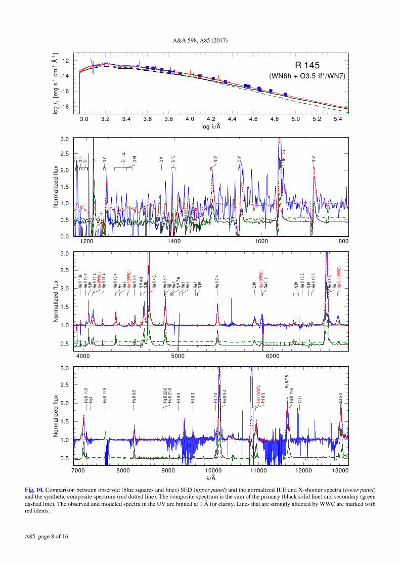
A comparison of the best-fitting models to the observed spec-tral energy distribution (SED) and normalized spectra is shownin Fig. 10. We note that the composite spectrum strongly under-predicts low-energy transitions such as He i lines. We show inSect. 7 that these lines are expected to be strongly contaminatedby WWC. The derived stellar parameters are listed in Table 2,where we also give the Smith and Johnson absolute magnitudesMv and MV , as well as the total extinction AV . We also give upperlimits derived for the projected and actual rotation velocity v sin iand vrot for both components, as derived by comparing linesformed close to the stellar surface (N iv λ4058, Si iv doublet)to synthetic spectra that account for rotation in an expanding at-mosphere, assuming corotation up to τRoss = 2/3 and angularmomentum conservation beyond (cf. Shenar et al. 2014). Giventhe low inclination angle, these only place weak constraints onthe actual rotation velocities vrot of the stars. Errors are estimatedfrom the sensitivity of the fit quality to variations of stellar pa-rameters, or through error propagation.

Table 2 also lists stellar masses that are based on mass-luminosity relations calculated by Gräfener et al. (2011) for ho-mogeneous stars. The relations depend on L and XH alone.MMLR,hom assumes the derived value of XH in the core, that is,a homogeneous star. MMLR,He−b assumes XH = 0, that is, the re-lation for pure He stars, which is a good approximation if thehydrogen-rich envelope is of negligible to moderate mass (see

A85, page 7 of 16

A&A 598, A85 (2017)

R 145(WN6h + O3.5 If*/WN7)

-18

-16

-14

-12

3.0 3.2 3.4 3.6 3.8 4.0 4.2 4.4 4.6 4.8 5.0 5.2 5.4

log λ/Ao

log

fλ [

erg

s-1

cm

-2 Ao

-1]

CIII

NIII

SIII

Lα NV

SII

i.s.

OV

I

OV

SiI

V

NIV

CIV

He

II 3-

2

NIV

0.0

0.5

1.0

1.5

2.0

2.5

3.0

1200 1400 1600 1800

No

rma

lize

d f

lux

He

II / H

εH

eII

13-4

NIV

He

II 12

-4H

δ (W

WC

)H

eII

11-4

He

II 10

-4H

γH

eI

He

I (W

WC

)

He

II 9-

4

NV

4-3

NIII

He

II 4-

3

He

II 8-

4H

βH

eI

NV

7-6

He

IH

eI

He

IN

IV

He

II 7-

4

CIV

He

I (W

WC

)N

aI i

.s.

NIV

He

II 16

-5

NIV

He

II 15

-5

He

II 6-

4H

αH

eII,

I (W

WC

)

0.5

1.0

1.5

2.0

2.5

3.0

4000 5000 6000

No

rma

lize

d f

lux

He

II 11

-5H

eI

He

II 11

-5

He

II 9-

5

He

II 22

-6H

eII

21-6

HI 9

-3

HI 8

-3

HI 7

-3

He

II 5-

4

He

I (W

WC

)H

I 6-3

He

II 7-

5H

eII

11-6

OV

I

HI 5

-3

0.5

1.0

1.5

2.0

2.5

3.0

7000 8000 9000 10000 11000 12000 13000

λ/Ao

No

rma

lize

d f

lux

Fig. 10. Comparison between observed (blue squares and lines) SED (upper panel) and the normalized IUE and X-shooter spectra (lower panel)and the synthetic composite spectrum (red dotted line). The composite spectrum is the sum of the primary (black solid line) and secondary (greendashed line). The observed and modeled spectra in the UV are binned at 1 Å for clarity. Lines that are strongly affected by WWC are marked withred idents.

A85, page 8 of 16

T. Shenar et al.: A first SB2 orbital and spectroscopic analysis for the Wolf-Rayet binary R145

Table 2. Derived physical parameters for R145.

Parameter Primary SecondarySpectral type WN6h O3.5 If*/WN7T∗ [K] 50 000 ± 3000 43 000 ± 3000log L [L] 6.35 ± 0.15 6.33 ± 0.15log Rt [R] 1.05 ± 0.05 1.50 ± 0.15v∞ [km s−1 ] 1200 ± 200 1000 ± 200R∗ [R] 20+6

−5 26+9−7

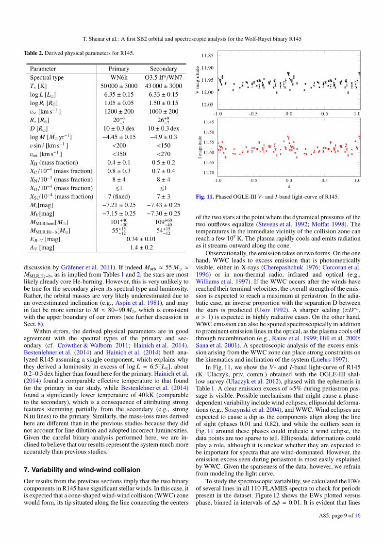
D [R] 10 ± 0.3 dex 10 ± 0.3 dexlog M [M yr−1] −4.45 ± 0.15 −4.9 ± 0.3v sin i [km s−1 ] <200 <150vrot [km s−1 ] <350 <270XH (mass fraction) 0.4 ± 0.1 0.5 ± 0.2XC/10−4 (mass fraction) 0.8 ± 0.3 0.7 ± 0.4XN/10−3 (mass fraction) 8 ± 4 8 ± 4XO/10−4 (mass fraction) .1 .1XSi/10−4 (mass fraction) 7 (fixed) 7 ± 3Mv[mag] −7.21 ± 0.25 −7.43 ± 0.25MV [mag] −7.15 ± 0.25 −7.30 ± 0.25MMLR,hom[M] 101+40

−30 109+60−40

MMLR,He−b[M] 55+15−12 54+15

−12EB−V [mag] 0.34 ± 0.01AV [mag] 1.4 ± 0.2

discussion by Gräfener et al. 2011). If indeed Morb ≈ 55 M ≈MMLR,He−b, as is implied from Tables 1 and 2, the stars are mostlikely already core He-burning. However, this is very unlikely tobe true for the secondary given its spectral type and luminosity.Rather, the orbital masses are very likely underestimated due toan overestimated inclination (e.g., Aspin et al. 1981), and mayin fact be more similar to M ≈ 80−90 M, which is consistentwith the upper boundary of our errors (see further discussion inSect. 8).

Within errors, the derived physical parameters are in goodagreement with the spectral types of the primary and sec-ondary (cf. Crowther & Walborn 2011; Hainich et al. 2014).Bestenlehner et al. (2014) and Hainich et al. (2014) both ana-lyzed R145 assuming a single component, which explains whythey derived a luminosity in excess of log L = 6.5 [L], about0.2–0.3 dex higher than found here for the primary. Hainich et al.(2014) found a comparable effective temperature to that foundfor the primary in our study, while Bestenlehner et al. (2014)found a significantly lower temperature of 40 kK (comparableto the secondary), which is a consequence of attributing strongfeatures stemming partially from the secondary (e.g., strongN iii lines) to the primary. Similarly, the mass-loss rates derivedhere are different than in the previous studies because they didnot account for line dilution and adopted incorrect luminosities.Given the careful binary analysis performed here, we are in-clined to believe that our results represent the system much moreaccurately than previous studies.

7. Variability and wind-wind collision

Our results from the previous sections imply that the two binarycomponents in R145 have significant stellar winds. In this case, itis expected that a cone-shaped wind-wind collision (WWC) zonewould form, its tip situated along the line connecting the centers

12.05

12.00

11.95

11.90

11.85

-1.0 -0.5 0.0 0.5 1.0

V m

ag

nit

ud

e

11.70

11.65

11.60

11.55

11.50

11.45

-1.0 -0.5 0.0 0.5 1.0

φ

I m

ag

nit

ud

eFig. 11. Phased OGLE-III V- and I-band light-curve of R145.

of the two stars at the point where the dynamical pressures of thetwo outflows equalize (Stevens et al. 1992; Moffat 1998). Thetemperatures in the immediate vicinity of the collision zone canreach a few 107 K. The plasma rapidly cools and emits radiationas it streams outward along the cone.

Observationally, the emission takes on two forms. On the onehand, WWC leads to excess emission that is photometricallyvisible, either in X-rays (Cherepashchuk 1976; Corcoran et al.1996) or in non-thermal radio, infrared and optical (e.g.,Williams et al. 1997). If the WWC occurs after the winds havereached their terminal velocities, the overall strength of the emis-sion is expected to reach a maximum at periastron. In the adia-batic case, an inverse proportion with the separation D betweenthe stars is predicted (Usov 1992). A sharper scaling (∝D−n,n > 1) is expected in highly radiative cases. On the other hand,WWC emission can also be spotted spectroscopically in additionto prominent emission lines in the optical, as the plasma cools offthrough recombination (e.g., Rauw et al. 1999; Hill et al. 2000;Sana et al. 2001). A spectroscopic analysis of the excess emis-sion arising from the WWC zone can place strong constraints onthe kinematics and inclination of the system (Luehrs 1997).

In Fig. 11, we show the V- and I-band light-curve of R145(K. Ulaczyk, priv. comm.) obtained with the OGLE-III shal-low survey (Ulaczyk et al. 2012), phased with the ephemeris inTable 1. A clear emission excess of ≈5% during periastron pas-sage is visible. Possible mechanisms that might cause a phase-dependent variability include wind eclipses, ellipsoidal deforma-tions (e.g., Soszynski et al. 2004), and WWC. Wind eclipses areexpected to cause a dip as the components align along the lineof sight (phases 0.01 and 0.82), and while the outliers seen inFig. 11 around these phases could indicate a wind eclipse, thedata points are too sparse to tell. Ellipsoidal deformations couldplay a role, although it is unclear whether they are expected tobe important for spectra that are wind-dominated. However, theemission excess seen during periastron is most easily explainedby WWC. Given the sparseness of the data, however, we refrainfrom modeling the light curve.

To study the spectroscopic variability, we calculated the EWsof several lines in all 110 FLAMES spectra to check for periodspresent in the dataset. Figure 12 shows the EWs plotted versusphase, binned in intervals of ∆φ = 0.01. It is evident that lines

A85, page 9 of 16

A&A 598, A85 (2017)

He II λ4200

-2.0

-2.5

-1.0 -0.5 0.0 0.5 1.0

EW

[Ao

]

N IV λ4058

-6.0

-6.5

-7.0

-1.0 -0.5 0.0 0.5 1.0

He I λ4471

-0.5

-1.0

-1.0 -0.5 0.0 0.5 1.0

EW

[Ao

]

Hγ-4.0

-4.5

-5.0

-5.5

-1.0 -0.5 0.0 0.5 1.0

N III λ4378

-0.4

-0.6

-0.8

-1.0 -0.5 0.0 0.5 1.0

EW

[Ao

]

Hδ-10

-12

-14

-1.0 -0.5 0.0 0.5 1.0

N III λ4513-1.4

-1.6

-1.8

-1.0 -0.5 0.0 0.5 1.0

φ

EW

[Ao

]

He II λ4541-2.8

-3.0

-3.2

-3.4

-3.6

-1.0 -0.5 0.0 0.5 1.0

φ

Fig. 12. EWs as a function of orbital phase φmeasured for selected linesin the FLAMES spectra, binned at ∆φ = 0.01 intervals.

-4.0

-4.5

-5.0

-5.5

-1.0 -0.5 0.0 0.5 1.0

φ

Eq

uiv

ale

nt

Wid

th [

Ao]

Fig. 13. Fits of the form A1 + B1 D−2 (blue curve), A2 + B2 D−1 (redcurve), and A3 + B3 D−α (green curve) to the data points describing theEW as a function of phase φ for the line Hγ.

associated with low ionization stages such as He i, N iii, andBalmer lines show a clear increase in the emission near peri-astron (φ = 0). The largest increase in flux (factor of two) is seenat the He i λ4471 transition, followed by an increase of ≈40% forHγ. This is significantly more that observed for the continuum(see Fig. 11). This behavior is not seen at all in the He ii λ4200

35455570100160300700

50%

10%

1%

0.1%

Period [d]

Porb

0

5

10

15

20

25

0.0 0.5 1.0 1.5 2.0

ω [10-6

s-1

]

PN

(ω)

Fig. 14. Periodogram of the EWs of the Hδ line. The periodogram wascalculated from ω = 2π/T to ω = πN0/T with a spacing 0.1/T , whereN0 is the number of data points and T the total time of the observation.Various false-alarm probability levels are marked.

and N iv λ4058 lines, but is seen in the He ii λ4541 line, possiblybecause it is blended with an N iii component.

In Fig. 13, we plot the same data points as in Fig. 12 for Hγ,but include three curves that correspond to functions of the formA1+B1 D−1(φ) , A2+B2 D−2(φ), and A3+B3 D−α(φ) with the con-stants Ai, Bi, and α chosen to minimize the sum of the squareddifferences χ2. When leaving the exponent α as a free parameter,we obtain α ≈ 0.25. A similar test for the N iii λ4378 line re-sults in α ≈ 1, while for the He ii λ4541 line, we obtain α ≈ 1.2.Given the intrinsic scatter in the EWs and the poor coverage dur-ing periastron, we cannot exclude the 1/D adiabatic dependencepredicted by Usov (1992).

We checked for periodic signals on the EWs of the linesshown in Fig. 12. In most cases, we find significant detections ofperiods that agree with the orbital period. The remaining periodsare found to be insignificant. In Fig. 14 a periodogram (Scargle1982; Horne & Baliunas 1986) is shown as an example. Themost prominent peak appears for a period of 158.9± 0.8 days, invery good agreement with the orbital period found (cf. Table 1).The occurrence of further apparently significant peaks is causedprimarily by spectral leakage that is due to the unevenly spaceddata (Horne & Baliunas 1986), as we confirmed by subtractingthe main signal and constructing a second periodogram. We finda marginal detection of a further period of P2 ≈ 21 d, which maybe related to stochastic variability in the system, but could alsobe spurious.

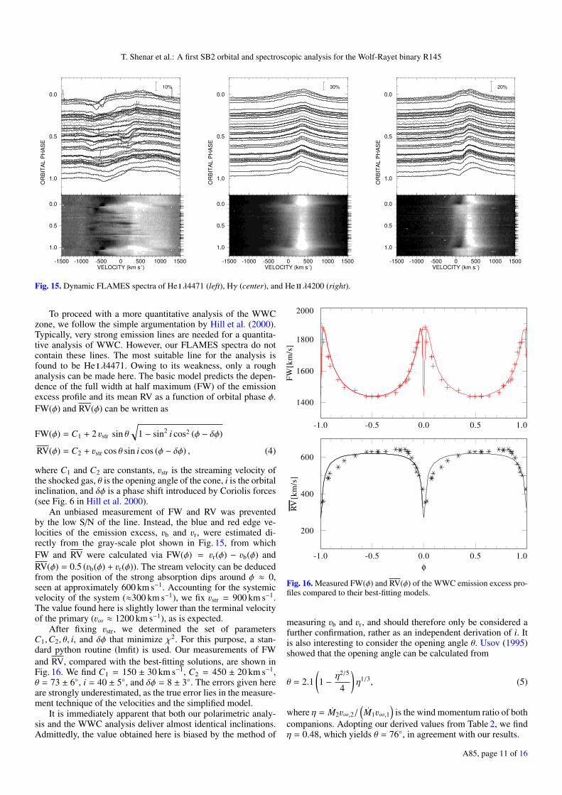
Figure 15 shows dynamic spectra calculated for three promi-nent lines: He i λ4471, H γ, and He ii λ4200. The He i image isespecially striking. There is a clear pattern of emission excesstraveling from ≈−600 km s−1 at φ ≈ 0 to ≈300 km s−1 at φ ≈ 0.7,and back again. This velocity amplitude clearly does not stemfrom the motion of the stars, which trace a different RV patternand move at amplitudes of ≈100 km s−1. In fact, the emissionpattern is fully consistent with a rotating WWC cone, as sug-gested by Luehrs (1997). The two strong absorption dips seenclose to periastron are also interesting; they likely occur whenthe cone arms tangentially sweep along the line of sight, therebyinstantaneously increasing the optical depth.

A85, page 10 of 16

T. Shenar et al.: A first SB2 orbital and spectroscopic analysis for the Wolf-Rayet binary R145

0.0

0.5

1.0

OR

BIT

AL

PH

AS

E

10%

-1500 -1000 -500 0 500 1000 1500VELOCITY (km s-1)

0.0

0.5

1.0

0.0

0.5

1.0

OR

BIT

AL

PH

AS

E

30%

-1500 -1000 -500 0 500 1000 1500VELOCITY (km s-1)

0.0

0.5

1.0

0.0

0.5

1.0

OR

BIT

AL

PH

AS

E

20%

-1500 -1000 -500 0 500 1000 1500VELOCITY (km s-1)

0.0

0.5

1.0

Fig. 15. Dynamic FLAMES spectra of He i λ4471 (left), Hγ (center), and He ii λ4200 (right).

To proceed with a more quantitative analysis of the WWCzone, we follow the simple argumentation by Hill et al. (2000).Typically, very strong emission lines are needed for a quantita-tive analysis of WWC. However, our FLAMES spectra do notcontain these lines. The most suitable line for the analysis isfound to be He i λ4471. Owing to its weakness, only a roughanalysis can be made here. The basic model predicts the depen-dence of the full width at half maximum (FW) of the emissionexcess profile and its mean RV as a function of orbital phase φ.FW(φ) and RV(φ) can be written as

FW(φ) = C1 + 2 vstr sin θ√

1 − sin2 i cos2 (φ − δφ)

RV(φ) = C2 + vstr cos θ sin i cos (φ − δφ) , (4)

where C1 and C2 are constants, vstr is the streaming velocity ofthe shocked gas, θ is the opening angle of the cone, i is the orbitalinclination, and δφ is a phase shift introduced by Coriolis forces(see Fig. 6 in Hill et al. 2000).

An unbiased measurement of FW and RV was preventedby the low S/N of the line. Instead, the blue and red edge ve-locities of the emission excess, vb and vr, were estimated di-rectly from the gray-scale plot shown in Fig. 15, from whichFW and RV were calculated via FW(φ) = vr(φ) − vb(φ) andRV(φ) = 0.5 (vb(φ) + vr(φ)). The stream velocity can be deducedfrom the position of the strong absorption dips around φ ≈ 0,seen at approximately 600 km s−1. Accounting for the systemicvelocity of the system (≈300 km s−1), we fix vstr = 900 km s−1.The value found here is slightly lower than the terminal velocityof the primary (v∞ ≈ 1200 km s−1), as is expected.

After fixing vstr, we determined the set of parametersC1,C2, θ, i, and δφ that minimize χ2. For this purpose, a stan-dard python routine (lmfit) is used. Our measurements of FWand RV, compared with the best-fitting solutions, are shown inFig. 16. We find C1 = 150 ± 30 km s−1, C2 = 450 ± 20 km s−1,θ = 73 ± 6, i = 40 ± 5, and δφ = 8 ± 3. The errors given hereare strongly underestimated, as the true error lies in the measure-ment technique of the velocities and the simplified model.

It is immediately apparent that both our polarimetric analy-sis and the WWC analysis deliver almost identical inclinations.Admittedly, the value obtained here is biased by the method of

1400

1600

1800

2000

-1.0 -0.5 0.0 0.5 1.0

FW

[km

/s]

200

400

600

-1.0 -0.5 0.0 0.5 1.0

φ

RV[k

m/s

]

Fig. 16. Measured FW(φ) and RV(φ) of the WWC emission excess pro-files compared to their best-fitting models.

measuring vb and vr, and should therefore only be considered afurther confirmation, rather as an independent derivation of i. Itis also interesting to consider the opening angle θ. Usov (1995)showed that the opening angle can be calculated from

θ = 2.1(1 − η

2/5

4

)η1/3, (5)

where η = M2v∞,2/(M1v∞,1

)is the wind momentum ratio of both

companions. Adopting our derived values from Table 2, we findη = 0.48, which yields θ = 76, in agreement with our results.

A85, page 11 of 16

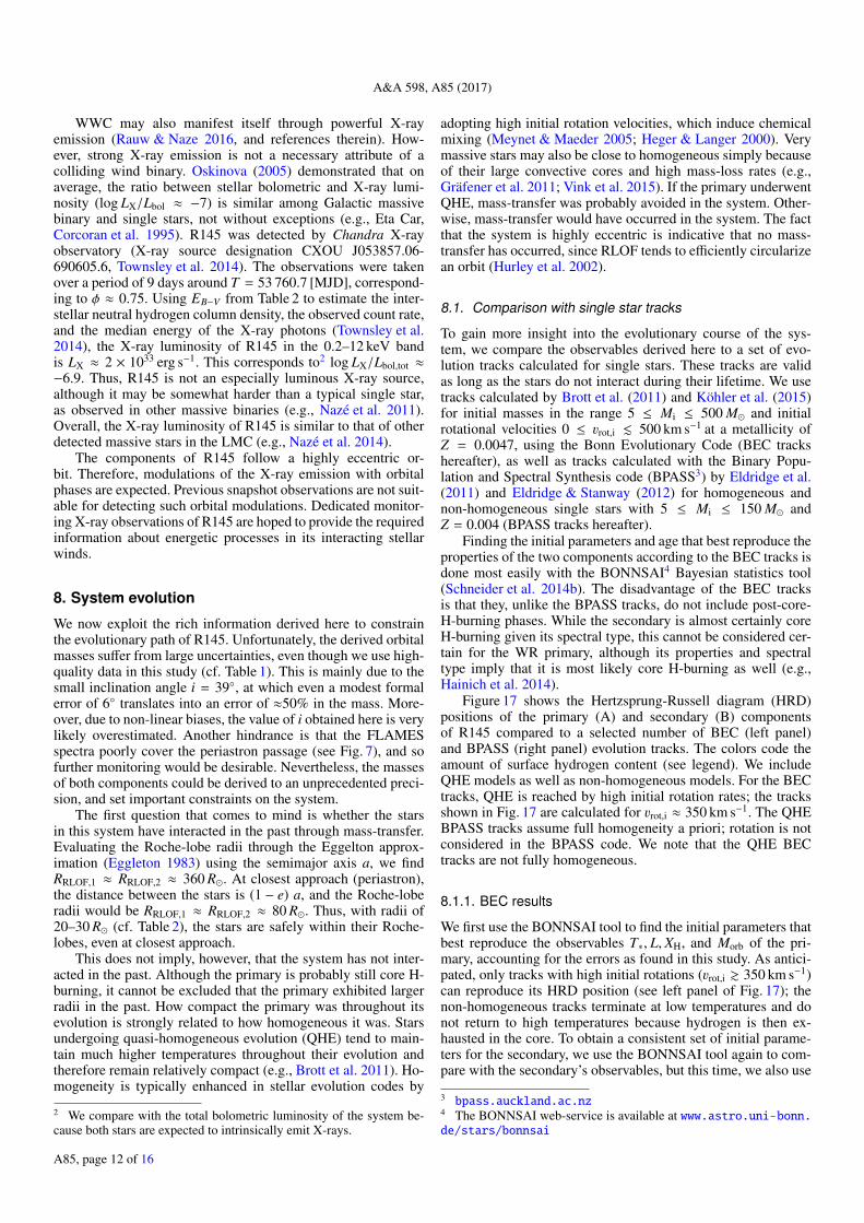
A&A 598, A85 (2017)

WWC may also manifest itself through powerful X-rayemission (Rauw & Naze 2016, and references therein). How-ever, strong X-ray emission is not a necessary attribute of acolliding wind binary. Oskinova (2005) demonstrated that onaverage, the ratio between stellar bolometric and X-ray lumi-nosity (log LX/Lbol ≈ −7) is similar among Galactic massivebinary and single stars, not without exceptions (e.g., Eta Car,Corcoran et al. 1995). R145 was detected by Chandra X-rayobservatory (X-ray source designation CXOU J053857.06-690605.6, Townsley et al. 2014). The observations were takenover a period of 9 days around T = 53 760.7 [MJD], correspond-ing to φ ≈ 0.75. Using EB−V from Table 2 to estimate the inter-stellar neutral hydrogen column density, the observed count rate,and the median energy of the X-ray photons (Townsley et al.2014), the X-ray luminosity of R145 in the 0.2–12 keV bandis LX ≈ 2 × 1033 erg s−1. This corresponds to2 log LX/Lbol,tot ≈−6.9. Thus, R145 is not an especially luminous X-ray source,although it may be somewhat harder than a typical single star,as observed in other massive binaries (e.g., Nazé et al. 2011).Overall, the X-ray luminosity of R145 is similar to that of otherdetected massive stars in the LMC (e.g., Nazé et al. 2014).

The components of R145 follow a highly eccentric or-bit. Therefore, modulations of the X-ray emission with orbitalphases are expected. Previous snapshot observations are not suit-able for detecting such orbital modulations. Dedicated monitor-ing X-ray observations of R145 are hoped to provide the requiredinformation about energetic processes in its interacting stellarwinds.

8. System evolution

We now exploit the rich information derived here to constrainthe evolutionary path of R145. Unfortunately, the derived orbitalmasses suffer from large uncertainties, even though we use high-quality data in this study (cf. Table 1). This is mainly due to thesmall inclination angle i = 39, at which even a modest formalerror of 6 translates into an error of ≈50% in the mass. More-over, due to non-linear biases, the value of i obtained here is verylikely overestimated. Another hindrance is that the FLAMESspectra poorly cover the periastron passage (see Fig. 7), and sofurther monitoring would be desirable. Nevertheless, the massesof both components could be derived to an unprecedented preci-sion, and set important constraints on the system.

The first question that comes to mind is whether the starsin this system have interacted in the past through mass-transfer.Evaluating the Roche-lobe radii through the Eggelton approx-imation (Eggleton 1983) using the semimajor axis a, we findRRLOF,1 ≈ RRLOF,2 ≈ 360 R. At closest approach (periastron),the distance between the stars is (1 − e) a, and the Roche-loberadii would be RRLOF,1 ≈ RRLOF,2 ≈ 80 R. Thus, with radii of20–30 R (cf. Table 2), the stars are safely within their Roche-lobes, even at closest approach.

This does not imply, however, that the system has not inter-acted in the past. Although the primary is probably still core H-burning, it cannot be excluded that the primary exhibited largerradii in the past. How compact the primary was throughout itsevolution is strongly related to how homogeneous it was. Starsundergoing quasi-homogeneous evolution (QHE) tend to main-tain much higher temperatures throughout their evolution andtherefore remain relatively compact (e.g., Brott et al. 2011). Ho-mogeneity is typically enhanced in stellar evolution codes by

2 We compare with the total bolometric luminosity of the system be-cause both stars are expected to intrinsically emit X-rays.

adopting high initial rotation velocities, which induce chemicalmixing (Meynet & Maeder 2005; Heger & Langer 2000). Verymassive stars may also be close to homogeneous simply becauseof their large convective cores and high mass-loss rates (e.g.,Gräfener et al. 2011; Vink et al. 2015). If the primary underwentQHE, mass-transfer was probably avoided in the system. Other-wise, mass-transfer would have occurred in the system. The factthat the system is highly eccentric is indicative that no mass-transfer has occurred, since RLOF tends to efficiently circularizean orbit (Hurley et al. 2002).

8.1. Comparison with single star tracks

To gain more insight into the evolutionary course of the sys-tem, we compare the observables derived here to a set of evo-lution tracks calculated for single stars. These tracks are validas long as the stars do not interact during their lifetime. We usetracks calculated by Brott et al. (2011) and Köhler et al. (2015)for initial masses in the range 5 ≤ Mi ≤ 500 M and initialrotational velocities 0 ≤ vrot,i . 500 km s−1 at a metallicity ofZ = 0.0047, using the Bonn Evolutionary Code (BEC trackshereafter), as well as tracks calculated with the Binary Popu-lation and Spectral Synthesis code (BPASS3) by Eldridge et al.(2011) and Eldridge & Stanway (2012) for homogeneous andnon-homogeneous single stars with 5 ≤ Mi ≤ 150 M andZ = 0.004 (BPASS tracks hereafter).

Finding the initial parameters and age that best reproduce theproperties of the two components according to the BEC tracks isdone most easily with the BONNSAI4 Bayesian statistics tool(Schneider et al. 2014b). The disadvantage of the BEC tracksis that they, unlike the BPASS tracks, do not include post-core-H-burning phases. While the secondary is almost certainly coreH-burning given its spectral type, this cannot be considered cer-tain for the WR primary, although its properties and spectraltype imply that it is most likely core H-burning as well (e.g.,Hainich et al. 2014).

Figure 17 shows the Hertzsprung-Russell diagram (HRD)positions of the primary (A) and secondary (B) componentsof R145 compared to a selected number of BEC (left panel)and BPASS (right panel) evolution tracks. The colors code theamount of surface hydrogen content (see legend). We includeQHE models as well as non-homogeneous models. For the BECtracks, QHE is reached by high initial rotation rates; the tracksshown in Fig. 17 are calculated for vrot,i ≈ 350 km s−1. The QHEBPASS tracks assume full homogeneity a priori; rotation is notconsidered in the BPASS code. We note that the QHE BECtracks are not fully homogeneous.

8.1.1. BEC results

We first use the BONNSAI tool to find the initial parameters thatbest reproduce the observables T∗, L, XH, and Morb of the pri-mary, accounting for the errors as found in this study. As antici-pated, only tracks with high initial rotations (vrot,i & 350 km s−1)can reproduce its HRD position (see left panel of Fig. 17); thenon-homogeneous tracks terminate at low temperatures and donot return to high temperatures because hydrogen is then ex-hausted in the core. To obtain a consistent set of initial parame-ters for the secondary, we use the BONNSAI tool again to com-pare with the secondary’s observables, but this time, we also use

3 bpass.auckland.ac.nz4 The BONNSAI web-service is available at www.astro.uni-bonn.de/stars/bonnsai

A85, page 12 of 16

T. Shenar et al.: A first SB2 orbital and spectroscopic analysis for the Wolf-Rayet binary R145

BEC

60 M

80 M

100 M

125 M

WC phase

WNE phase

WNL phase

pre WR phase

A

B

< 5 % H

5 − 30 % H

30 − 50 % H

> 50 % H

T*

/kK

10204060100

QHE non-hom.

ZAMSzero age mainsequence

5.6

5.8

6.0

6.2

6.4

6.6

5.0 4.5 4.0 3.5

log (T*

/K)

log

(L

/L)

BPASS

60M

80M

100M

120MA

B

T*

/kK

10204060100150200

QHE non-hom.

ZAMSzero age mainsequence

5.6

5.8

6.0

6.2

6.4

6.6

5.0 4.5 4.0 3.5

log (T*

/K)

log

(L

/L)

Fig. 17. HRD positions of the primary (A) and secondary (B) components of R145 compared to BEC (left panel) and BPASS (right panel) evolutiontracks calculated for (near-)homogeneous and non-homogeneous evolution for LMC metallicities. The WR phase is defined for XH < 0.65 andT∗ > 20 kK. See text for details.

the primary age (and associated errors), as obtained from theBONNSAI tool.

The resulting initial masses and age (as derived for the pri-mary) are shown in Table 3. The Table also lists the currentmasses and hydrogen content of the two components as pre-dicted from the best-fitting evolutionary track. The initial rota-tions obtained by the BONNSAI tool for the primary and sec-ondary are vrot,i = 410 and 340 km s−1, respectively, while thepredicted current rotational velocities are 240 and 260 km s−1,marginally consistent with the upper bounds given in Table 2.Since the non-homogeneous BEC models do not reproduce theHRD positions of the system components, we list only the cor-responding QHE solution in Table 3.

8.1.2. BPASS results

A similar procedure is performed with the BPASS tracks. Weuse a χ2 minimization algorithm to find the best-fitting homo-geneous and non-homogeneous tracks and ages that reproducethe properties of the primary (see Eq. (3) in Shenar et al. 2016).Once a track and age for the primary is inferred, we repeat theprocedure for the secondary, adopting the primary’s age an as-sociated error estimate that is based on the grid spacing. Thecorresponding initial parameters, ages, and current mass and sur-face hydrogen content are listed in Table 3. Because the BPASStracks cover the whole evolution of the star, appropriate solu-tions can be found for the non-homogeneous case as well (seealso right panel of Fig. 17). In Table 3 we also list the maximumradius Rmax,1 reached by the primary throughout its evolution.This is meant to indicate whether the primary has exceeded itsRoche-lobe radius in the past.

8.1.3. Indication of QHE

The BEC tracks and the BPASS tracks imply very similar initialparameters and ages in the QHE case for the two components.The tracks reproduce the observables reasonably well (comparedto the errors), but the current masses predicted by the evolution-ary tracks (≈80−90 M) are higher than the orbital masses de-rived here (≈55 M). Such masses would be obtained at an in-clination of ≈33, which is roughly consistent with our formalerror on i given in Table 1. The QHE scenario would thereforesuggest that the actual masses are ≈80−90 M per component.

For the non-QHE scenario, only the BPASS tracks can placemeaningful constraints. In this scenario, the properties of the pri-mary are reproduced when the evolution tracks return from thered to the blue, and He-core burning is initiated. This scenariois consistent with much lower current masses, closer to thosederived here. However, significant discrepancy is obtained forthe hydrogen content. More importantly, a comparison betweenthe maximum radius reached by the primary and the Roche-lobe implies that when we adopt the non-homogeneous tracks,the primary overfilled its Roche-lobe in the past. We note thatthe separation increases with time because of mass-loss, makingmass-transfer inevitable in the non-homogeneous case. In thisscenario, binary interaction therefore has to be accounted for.

8.2. Binary tracks

We now use the set of tracks calculated with version 2.0 ofthe BPASS code (Eldridge et al. 2008) for Z = 0.004, whichare non-homogeneous and account for mass-transfer. Each trackis defined by an initial period Pi, an initial mass ratio qi =Mi,2/Mi,1, and an initial mass for the primary Mi,1, calculatedat intervals of 0.2 on 0 < log P [d] < 4, 0.2 on 0 < qi < 0.9, and10–20 M on 10 < Mi,1 < 150 M. The tracks do not include

A85, page 13 of 16

A&A 598, A85 (2017)

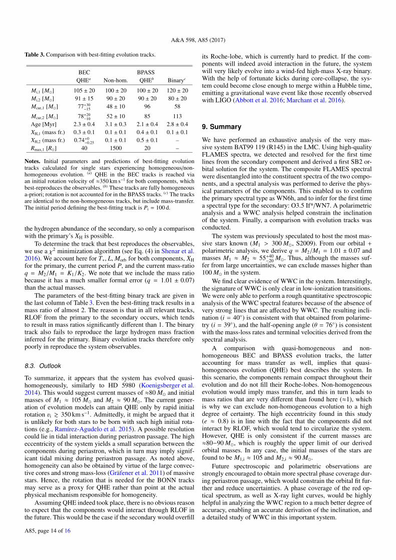
Table 3. Comparison with best-fitting evolution tracks.

BEC BPASSQHEa Non-hom. QHEb Binaryc

Mi,1 [M] 105 ± 20 100 ± 20 100 ± 20 120 ± 20Mi,2 [M] 91 ± 15 90 ± 20 90 ± 20 80 ± 20Mcur,1 [M] 77+30

−15 48 ± 10 96 58

Mcur,2 [M] 78+20−10 52 ± 10 85 113

Age [Myr] 2.3 ± 0.4 3.1 ± 0.3 2.1 ± 0.4 2.8 ± 0.4XH,1 (mass fr.) 0.3 ± 0.1 0.1 ± 0.1 0.4 ± 0.1 0.1 ± 0.1XH,2 (mass fr.) 0.74+0

−0.25 0.1 ± 0.1 0.5 ± 0.1 –Rmax,1 [R] 40 1500 20 –

Notes. Initial parameters and predictions of best-fitting evolutiontracks calculated for single stars experiencing homogeneous/non-homogeneous evolution. (a) QHE in the BEC tracks is reached viaan initial rotation velocity of ≈350 km s−1 for both components, whichbest-reproduces the observables. (b) These tracks are fully homogeneousa-priori; rotation is not accounted for in the BPASS tracks. (c) The tracksare identical to the non-homogeneous tracks, but include mass-transfer.The initial period defining the best-fitting track is Pi = 100 d.

the hydrogen abundance of the secondary, so only a comparisonwith the primary’s XH is possible.

To determine the track that best reproduces the observables,we use a χ2 minimization algorithm (see Eq. (4) in Shenar et al.2016). We account here for T∗, L,Morb for both components, XHfor the primary, the current period P, and the current mass-ratioq = M2/M1 = K1/K2. We note that we include the mass ratiobecause it has a much smaller formal error (q = 1.01 ± 0.07)than the actual masses.

The parameters of the best-fitting binary track are given inthe last column of Table 3. Even the best-fitting track results in amass ratio of almost 2. The reason is that in all relevant tracks,RLOF from the primary to the secondary occurs, which tendsto result in mass ratios significantly different than 1. The binarytrack also fails to reproduce the large hydrogen mass fractioninferred for the primary. Binary evolution tracks therefore onlypoorly in reproduce the system observables.

8.3. Outlook

To summarize, it appears that the system has evolved quasi-homogeneously, similarly to HD 5980 (Koenigsberger et al.2014). This would suggest current masses of ≈80 M and initialmasses of M1 ≈ 105 M and M2 ≈ 90 M. The current gener-ation of evolution models can attain QHE only by rapid initialrotation vi & 350 km s−1. Admittedly, it might be argued that itis unlikely for both stars to be born with such high initial rota-tions (e.g., Ramírez-Agudelo et al. 2015). A possible resolutioncould lie in tidal interaction during periastron passage. The higheccentricity of the system yields a small separation between thecomponents during periastron, which in turn may imply signif-icant tidal mixing during periastron passage. As noted above,homogeneity can also be obtained by virtue of the large convec-tive cores and strong mass-loss (Gräfener et al. 2011) of massivestars. Hence, the rotation that is needed for the BONN tracksmay serve as a proxy for QHE rather than point at the actualphysical mechanism responsible for homogeneity.

Assuming QHE indeed took place, there is no obvious reasonto expect that the components would interact through RLOF inthe future. This would be the case if the secondary would overfill

its Roche-lobe, which is currently hard to predict. If the com-ponents will indeed avoid interaction in the future, the systemwill very likely evolve into a wind-fed high-mass X-ray binary.With the help of fortunate kicks during core-collapse, the sys-tem could become close enough to merge within a Hubble time,emitting a gravitational wave event like those recently observedwith LIGO (Abbott et al. 2016; Marchant et al. 2016).

9. Summary

We have performed an exhaustive analysis of the very mas-sive system BAT99 119 (R145) in the LMC. Using high-qualityFLAMES spectra, we detected and resolved for the first timelines from the secondary component and derived a first SB2 or-bital solution for the system. The composite FLAMES spectralwere disentangled into the constituent spectra of the two compo-nents, and a spectral analysis was performed to derive the phys-ical parameters of the components. This enabled us to confirmthe primary spectral type as WN6h, and to infer for the first timea spectral type for the secondary: O3.5 If*/WN7. A polarimetricanalysis and a WWC analysis helped constrain the inclinationof the system. Finally, a comparison with evolution tracks wasconducted.

The system was previously speculated to host the most mas-sive stars known (M1 > 300 M, S2009). From our orbital +polarimetric analysis, we derive q = M2/M1 = 1.01 ± 0.07 andmasses M1 ≈ M2 ≈ 55+40

−20 M. Thus, although the masses suf-fer from large uncertainties, we can exclude masses higher than100 M in the system.

We find clear evidence of WWC in the system. Interestingly,the signature of WWC is only clear in low-ionization transitions.We were only able to perform a rough quantitative spectroscopicanalysis of the WWC spectral features because of the absence ofvery strong lines that are affected by WWC. The resulting incli-nation (i = 40) is consistent with that obtained from polarime-try (i = 39), and the half-opening angle (θ = 76) is consistentwith the mass-loss rates and terminal velocities derived from thespectral analysis.

A comparison with quasi-homogeneous and non-homogeneous BEC and BPASS evolution tracks, the latteraccounting for mass transfer as well, implies that quasi-homogeneous evolution (QHE) best describes the system. Inthis scenario, the components remain compact throughout theirevolution and do not fill their Roche-lobes. Non-homogeneousevolution would imply mass transfer, and this in turn leads tomass ratios that are very different than found here (≈1), whichis why we can exclude non-homogeneous evolution to a highdegree of certainty. The high eccentricity found in this study(e ≈ 0.8) is in line with the fact that the components did notinteract by RLOF, which would tend to circularize the system.However, QHE is only consistent if the current masses are≈80−90 M, which is roughly the upper limit of our derivedorbital masses. In any case, the initial masses of the stars arefound to be M1,i ≈ 105 and M2,i ≈ 90 M.

Future spectroscopic and polarimetric observations arestrongly encouraged to obtain more spectral phase coverage dur-ing periastron passage, which would constrain the orbital fit fur-ther and reduce uncertainties. A phase coverage of the red op-tical spectrum, as well as X-ray light curves, would be highlyhelpful in analyzing the WWC region to a much better degree ofaccuracy, enabling an accurate derivation of the inclination, anda detailed study of WWC in this important system.

A85, page 14 of 16

T. Shenar et al.: A first SB2 orbital and spectroscopic analysis for the Wolf-Rayet binary R145

Acknowledgements. We are grateful for the constructive comments of our ref-eree. T.S. acknowledges the financial support from the Leibniz Graduate Schoolfor Quantitative Spectroscopy in Astrophysics, a joint project of the Leibniz In-stitute for Astrophysics Potsdam (AIP) and the institute of Physics and Astron-omy of the University of Potsdam. A.F.J.M. is grateful for financial aid fromNSERC (Canada) and FQRNT (Quebec). N.D.R. is grateful for postdoctoralsupport by the University of Toledo and by the Helen Luedke Brooks EndowedProfessorship. L.A.A. acknowledges support from the Fundacão de Amparo àPesquisa do Estado de São Paulo – FAPESP (2013/18245-0 and 2012/09716-6).R.H.B. thanks for support from FONDECYT project No. 1140076.

ReferencesAbbott, B. P., Abbott, R., Abbott, T. D., et al. 2016, Phys. Rev. Lett., 116, 061102Aldoretta, E. J., Caballero-Nieves, S. M., Gies, D. R., et al. 2015, AJ, 149, 26Almeida, L. A., Sana, H., Taylor, W., et al. 2017, A&A, 598, A84 (Paper I)Andersen, J. 1991, A&ARv, 3, 91Aspin, C., Simmons, J. F. L., & Brown, J. C. 1981, MNRAS, 194, 283Banerjee, S., Kroupa, P., & Oh, S. 2012, ApJ, 746, 15Bestenlehner, J. M., Vink, J. S., Gräfener, G., et al. 2011, A&A, 530, L14Bestenlehner, J. M., Gräfener, G., Vink, J. S., et al. 2014, A&A, 570, A38Bonanos, A. Z. 2009, ApJ, 691, 407Bonanos, A. Z., Stanek, K. Z., Udalski, A., et al. 2004, ApJ, 611, L33Bonanos, A. Z., Lennon, D. J., Köhlinger, F., et al. 2010, AJ, 140, 416Bonnell, I. A., Bate, M. R., Clarke, C. J., & Pringle, J. E. 1997, MNRAS, 285,

201Breysacher, J., Azzopardi, M., & Testor, G. 1999, A&AS, 137, 117Brott, I., Evans, C. J., Hunter, I., et al. 2011, A&A, 530, A116Brown, J. C., McLean, I. S., & Emslie, A. G. 1978, A&A, 68, 415Brown, J. C., Aspin, C., Simmons, J. F. L., & McLean, I. S. 1982, MNRAS, 198,

787Castor, J. I., Abbott, D. C., & Klein, R. I. 1975, ApJ, 195, 157Cherepashchuk, A. M. 1976, Sov. Astron. Lett., 2, 138Corcoran, M. F., Rawley, G. L., Swank, J. H., & Petre, R. 1995, ApJ, 445, L121Corcoran, M. F., Stevens, I. R., Pollock, A. M. T., et al. 1996, ApJ, 464, 434Crowther, P. A., Schnurr, O., Hirschi, R., et al. 2010, MNRAS, 408, 731Crowther, P. A., & Walborn, N. R. 2011, MNRAS, 416, 1311Cutri, R. M., et al. 2013, VizieR Online Data Catalog: II/328de Mink, S. E., Sana, H., Langer, N., Izzard, R. G., & Schneider, F. R. N. 2014,

ApJ, 782, 7Eggleton, P. P. 1983, ApJ, 268, 368Eldridge, J. J., & Stanway, E. R. 2012, MNRAS, 419, 479Eldridge, J. J., Izzard, R. G., & Tout, C. A. 2008, MNRAS, 384, 1109Eldridge, J. J., Langer, N., & Tout, C. A. 2011, MNRAS, 414, 3501Evans, C. J., Taylor, W. D., Hénault-Brunet, V., et al. 2011, A&A, 530, A108Giménez-García, A., Shenar, T., Torrejón, J. M., et al. 2016, A&A, 591, A26Gosset, E., Royer, P., Rauw, G., Manfroid, J., & Vreux, J.-M. 2001, MNRAS,

327, 435Gräfener, G., Koesterke, L., & Hamann, W.-R. 2002, A&A, 387, 244Gräfener, G., Vink, J. S., de Koter, A., & Langer, N. 2011, A&A, 535, A56Hadrava, P. 1995, A&AS, 114, 393Hadrava, P., Šlechta, M., & Škoda, P. 2009, A&A, 507, 397Hainich, R., Rühling, U., Todt, H., et al. 2014, A&A, 565, A27Hamann, W.-R., & Gräfener, G. 2004, A&A, 427, 697Hamann, W.-R., & Koesterke, L. 1998, A&A, 335, 1003Hamann, W.-R., Gräfener, G., & Liermann, A. 2006, A&A, 457, 1015Heger, A., & Langer, N. 2000, ApJ, 544, 1016Hill, G. M., Moffat, A. F. J., St-Louis, N., & Bartzakos, P. 2000, MNRAS, 318,

402Hillier, D. J. 1984, ApJ, 280, 744Horne, J. H., & Baliunas, S. L. 1986, ApJ, 302, 757Howarth, I. D. 1983, MNRAS, 203, 301Hurley, J. R., Tout, C. A., & Pols, O. R. 2002, MNRAS, 329, 897Koenigsberger, G., Morrell, N., Hillier, D. J., et al. 2014, AJ, 148, 62Köhler, K., Langer, N., de Koter, A., et al. 2015, A&A, 573, A71Korn, A. J., Becker, S. R., Gummersbach, C. A., & Wolf, B. 2000, A&A, 353,

655Kroupa, P. 2001, MNRAS, 322, 231Lamontagne, R., Moffat, A. F. J., Drissen, L., Robert, C., & Matthews, J. M.

1996, AJ, 112, 2227Langer, N. 2012, ARA&A, 50, 107Luehrs, S. 1997, PASP, 109, 504

Magalhaes, A. M., Benedetti, E., & Roland, E. H. 1984, PASP, 96, 383Maíz Apellániz, J. 2010, A&A, 518, A1Maíz Apellániz, J., Evans, C. J., Barbá, R. H., et al. 2014, A&A, 564, A63Marchant, P., Langer, N., Podsiadlowski, P., Tauris, T. M., & Moriya, T. J. 2016,

A&A, 588, A50Mason, B. D., Hartkopf, W. I., Gies, D. R., Henry, T. J., & Helsel, J. W. 2009,

AJ, 137, 3358Massey, P., & Hunter, D. A. 1998, ApJ, 493, 180Meynet, G., & Maeder, A. 2005, A&A, 429, 581Moffat, A. F. J. 1989, ApJ, 347, 373Moffat, A. F. J. 1998, Ap&SS, 260, 225Moffat, A. F. J., Marchenko, S. V., Bartzakos, P., et al. 1998, ApJ, 497, 896Nazé, Y., Broos, P. S., Oskinova, L., et al. 2011, ApJS, 194, 7Nazé, Y., Petit, V., Rinbrand, M., et al. 2014, ApJS, 215, 10Niemela, V. S., Gamen, R. C., Barbá, R. H., et al. 2008, MNRAS, 389, 1447Oey, M. S., & Clarke, C. J. 2005, ApJ, 620, L43Oskinova, L. M. 2005, MNRAS, 361, 679Oskinova, L. M., Steinke, M., Hamann, W.-R., et al. 2013, MNRAS, 436, 3357Oudmaijer, R. D., & Parr, A. M. 2010, MNRAS, 405, 2439Paczynski, B. 1973, in Wolf-Rayet and High-Temperature Stars, eds. M. K. V.

Bappu, & J. Sahade, IAU Symp., 49, 143Parker, J. W., Garmany, C. D., Massey, P., & Walborn, N. R. 1992, AJ, 103, 1205Pietrzynski, G., Graczyk, D., Gieren, W., et al. 2013, Nature, 495, 76Ramírez-Agudelo, O. H., Sana, H., de Mink, S. E., et al. 2015, A&A, 580, A92Rauw, G., & Naze, Y. 2016, Adv. Space Res., 58, 761Rauw, G., Vreux, J.-M., Gosset, E., et al. 1996, A&A, 306, 771Rauw, G., Vreux, J.-M., & Bohannan, B. 1999, ApJ, 517, 416Rauw, G., De Becker, M., Nazé, Y., et al. 2004, A&A, 420, L9Robert, C., Moffat, A. F. J., Drissen, L., et al. 1992, ApJ, 397, 277Sablowski, D. P., & Weber, M. 2017, A&A, 597, A125Salpeter, E. E. 1955, ApJ, 121, 161Sana, H., Rauw, G., & Gosset, E. 2001, A&A, 370, 121Sana, H., de Mink, S. E., de Koter, A., et al. 2012, Science, 337, 444Sana, H., Le Bouquin, J.-B., Lacour, S., et al. 2014, ApJS, 215, 15Sander, A., Shenar, T., Hainich, R., et al. 2015, A&A, 577, A13Scargle, J. D. 1982, ApJ, 263, 835Schmutz, W., Hamann, W.-R., & Wessolowski, U. 1989, A&A, 210, 236Schneider, F. R. N., Izzard, R. G., de Mink, S. E., et al. 2014a, ApJ, 780, 117Schneider, F. R. N., Langer, N., de Koter, A., et al. 2014b, A&A, 570, A66Schnurr, O., Casoli, J., Chené, A.-N., Moffat, A. F. J., & St-Louis, N. 2008a,

MNRAS, 389, L38Schnurr, O., Moffat, A. F. J., St-Louis, N., Morrell, N. I., & Guerrero, M. A.

2008b, MNRAS, 389, 806Schnurr, O., Moffat, A. F. J., Villar-Sbaffi, A., St-Louis, N., & Morrell, N. I.

2009, MNRAS, 395, 823Shenar, T., Hamann, W.-R., & Todt, H. 2014, A&A, 562, A118Shenar, T., Oskinova, L., Hamann, W.-R., et al. 2015, ApJ, 809, 135Shenar, T., Hainich, R., Todt, H., et al. 2016, A&A, 591, A22Simmons, J. F. L., & Boyle, C. B. 1984, A&A, 134, 368Soszynski, I., Udalski, A., Kubiak, M., et al. 2004, Acta Astron., 54, 347Sota, A., Maíz Apellániz, J., Morrell, N. I., et al. 2014, ApJS, 211, 10St.-Louis, N., Moffat, A. F. J., Drissen, L., Bastien, P., & Robert, C. 1988, ApJ,

330, 286Stahl, O., Buzzoni, B., Kraus, G., et al. 1986, The Messenger, 46, 23Stevens, I. R., Blondin, J. M., & Pollock, A. M. T. 1992, ApJ, 386, 265Todt, H., Sander, A., Hainich, R., et al. 2015, A&A, 579, A75Torres, G., Andersen, J., & Giménez, A. 2010, A&ARv, 18, 67Townsley, L. K., Broos, P. S., Garmire, G. P., et al. 2014, ApJS, 213, 1Tramper, F., Sana, H., Fitzsimons, N. E., et al. 2016, MNRAS, 455, 1275Trundle, C., Dufton, P. L., Hunter, I., et al. 2007, A&A, 471, 625Ulaczyk, K., Szymanski, M. K., Udalski, A., et al. 2012, Acta Astron., 62, 247Usov, V. V. 1992, ApJ, 389, 635Usov, V. V. 1995, in Wolf-Rayet Stars: Binaries; Colliding Winds; Evolution,

eds. K. A. van der Hucht, & P. M. Williams, IAU Symp., 163, 495Vanbeveren, D., De Loore, C., & Van Rensbergen, W. 1998, A&ARv, 9, 63Vernet, J., Dekker, H., D’Odorico, S., et al. 2011, A&A, 536, A105Vink, J. S. 2015, Very Massive Stars in the Local Universe, Astrophysics and

Space Science Library, 412Vink, J. S., Heger, A., Krumholz, M. R., et al. 2015, Highlights of Astronomy,

16, 51Williams, P. M., Dougherty, S. M., Davis, R. J., et al. 1997, MNRAS, 289, 10Wolinski, K. G., & Dolan, J. F. 1994, MNRAS, 267, 5Zacharias, N., Finch, C. T., Girard, T. M., et al. 2012, VizieR Online Data

Catalog: I/322

A85, page 15 of 16

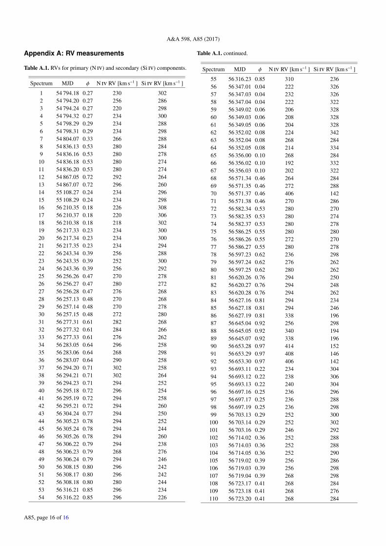
A&A 598, A85 (2017)

Appendix A: RV measurements

Table A.1. RVs for primary (N iv) and secondary (Si iv) components.

Spectrum MJD φ N iv RV [km s−1 ] Si iv RV [km s−1 ]

1 54 794.18 0.27 230 3022 54 794.20 0.27 256 2863 54 794.24 0.27 220 2984 54 794.32 0.27 234 3005 54 798.29 0.29 234 2886 54 798.31 0.29 234 2987 54 804.07 0.33 266 2888 54 836.13 0.53 280 2849 54 836.16 0.53 280 278

10 54 836.18 0.53 280 27411 54 836.20 0.53 280 27412 54 867.05 0.72 292 26413 54 867.07 0.72 296 26014 55 108.27 0.24 234 29615 55 108.29 0.24 234 29816 56 210.35 0.18 226 30817 56 210.37 0.18 220 30618 56 210.38 0.18 218 30219 56 217.33 0.23 234 30020 56 217.34 0.23 234 30021 56 217.35 0.23 234 29422 56 243.34 0.39 256 28823 56 243.35 0.39 252 30024 56 243.36 0.39 256 29225 56 256.26 0.47 270 27826 56 256.27 0.47 280 27227 56 256.28 0.47 276 26828 56 257.13 0.48 270 26829 56 257.14 0.48 270 27830 56 257.15 0.48 272 28031 56 277.31 0.61 282 26832 56 277.32 0.61 284 26633 56 277.33 0.61 276 26234 56 283.05 0.64 296 25835 56 283.06 0.64 268 29836 56 283.07 0.64 290 25837 56 294.20 0.71 302 25838 56 294.21 0.71 302 26439 56 294.23 0.71 294 25240 56 295.18 0.72 296 25441 56 295.19 0.72 294 25842 56 295.21 0.72 294 26043 56 304.24 0.77 294 25044 56 305.23 0.78 294 25245 56 305.24 0.78 294 24446 56 305.26 0.78 294 26047 56 306.22 0.79 294 23848 56 306.23 0.79 268 27649 56 306.24 0.79 294 24650 56 308.15 0.80 296 24251 56 308.17 0.80 296 24252 56 308.18 0.80 280 24453 56 316.21 0.85 296 23454 56 316.22 0.85 296 226

Table A.1. continued.

Spectrum MJD φ N iv RV [km s−1 ] Si iv RV [km s−1 ]

55 56 316.23 0.85 310 23656 56 347.01 0.04 222 32657 56 347.03 0.04 232 32658 56 347.04 0.04 222 32259 56 349.02 0.06 206 32860 56 349.03 0.06 208 32861 56 349.05 0.06 204 32862 56 352.02 0.08 224 34263 56 352.04 0.08 268 28464 56 352.05 0.08 214 33465 56 356.00 0.10 268 28466 56 356.02 0.10 192 33267 56 356.03 0.10 202 32268 56 571.34 0.46 264 28469 56 571.35 0.46 272 28870 56 571.37 0.46 406 14271 56 571.38 0.46 270 28672 56 582.34 0.53 280 27073 56 582.35 0.53 280 27474 56 582.37 0.53 280 27875 56 586.25 0.55 280 28076 56 586.26 0.55 272 27077 56 586.27 0.55 280 27878 56 597.23 0.62 236 29879 56 597.24 0.62 276 26280 56 597.25 0.62 280 26281 56 620.26 0.76 294 25082 56 620.27 0.76 294 24883 56 620.28 0.76 294 26284 56 627.16 0.81 294 23485 56 627.18 0.81 294 24686 56 627.19 0.81 338 19687 56 645.04 0.92 256 29888 56 645.05 0.92 340 19489 56 645.07 0.92 338 19690 56 653.28 0.97 414 15291 56 653.29 0.97 408 14692 56 653.30 0.97 406 14293 56 693.11 0.22 234 30494 56 693.12 0.22 238 30695 56 693.13 0.22 240 30496 56 697.16 0.25 236 29697 56 697.17 0.25 236 28898 56 697.19 0.25 236 29899 56 703.13 0.29 252 300

100 56 703.14 0.29 252 302101 56 703.16 0.29 246 292102 56 714.02 0.36 252 288103 56 714.03 0.36 252 288104 56 714.05 0.36 252 290105 56 719.02 0.39 256 286106 56 719.03 0.39 256 298107 56 719.04 0.39 268 298108 56 723.17 0.41 268 284109 56 723.18 0.41 268 276110 56 723.20 0.41 268 284

A85, page 16 of 16