applied sciences

Article

Tarantula: Design, Modeling, and KinematicIdentification of a Quadruped Wheeled Robot

Abdullah Aamir Hayat 1,* , Karthikeyan Elangovan 1, Mohan Rajesh Elara 1 andMullapudi Sai Teja 1,2

1 Engineering Product Development Pillar, Singapore University of Technology and Design (SUTD),Singapore 487372, Singapore; e_karthikeyan@sutd.edu.sg (K.E.); rajeshelara@sutd.edu.sg (M.R.E.),mullapudisai1812@gmail.com (M.S.T.)

2 Department of Mechanical Engineering, Politecnico di Milano, 20133 Milan, Italy* Correspondence: abdullahaamir@sutd.edu.sg

Received: 7 November 2018; Accepted: 17 December 2018; Published: 27 December 2018 �����������������

Abstract: This paper firstly presents the design and modeling of a quadruped wheeled robot namedTarantula. It has four legs each having four degrees of freedom with a proximal end attached tothe trunk and the wheels for locomotion connected at the distal end. The two legs in the front andtwo at the back are actuated using two motors which are placed inside the trunk for simultaneousabduction or adduction. It is designed to manually reconfigure its topology as per the cross-sectionsof the drainage system. The bi-directional suspension system is designed using a single damper toprevent the trunk and inside components from shock. Formulation for kinematics of the wheels thatis coupled with the kinematics of each leg is presented. We proposed the cost-effective method whichis also an on-site approach to estimate the kinematic parameters and the effective trunk dimensionafter assembly of the quadruped robot using the monocular camera and ArUco markers insteadof high-end devices like a laser tracker or coordinate measurement machine. The measurementtechnique is evaluated experimentally and the same set up was used for trajectory tracking of theTarantula. The experimental method for the kinematic identification presented here can be easilyextended to the other mobile robots with serial architecture designed legs.

Keywords: design and modeling; kinematics; kinematic identification; monocular vision

1. Introduction

Drains are an integral part of every modern city, where drainage systems are entirely subsurfacein most countries. Statistics from Asia, Europe, United States show that major cities contain 4000 to7000 km of drainage lines. The primary purpose of these surface and subsurface sewage systems is toremove excess water in a safe and timely manner, which plays a vital role in controlling water-relateddiseases or water-borne diseases. Drainage systems have its disadvantages, where these systemsgive problems to mosquito-borne diseases, clogging, internal damages due to ageing, excessive trafficwhich causes contamination of groundwater or overflow. To control these problems, serious inspection,monitoring and maintenance of drainage systems is required. At present, this task is labor-intensive asshown in Figure 1a that adds more difficulties in subsurface sewer lines like inaccessible areas withpoor lighting, ventilation and safety concerns associated with insect bites. The cross-section of thedrainage system with the approximate symmetric design shown in Figure 1b are widely found inSingapore [1]. The width, W, of these drainages typically range from 1.1 to 1.8 m, w from 0.2–0.8 mand the height h between 0.3–1.1 m. Thus, there is a requirement to design the robot to traverse insidethis type of drainage systems.

Appl. Sci. 2018, 9, 94; doi:10.3390/app9010094 www.mdpi.com/journal/applsci

Appl. Sci. 2018, 9, 94 2 of 21

w

b 1d

W

V - typeU - type

a) Human collecting sample b) Cross-section of drainage

incl

inat

ion

h

Figure 1. Human collecting water samples inside the drain commonly found in Singapore [1].

The specially designed mechanism with suited locomotion as per the internal geometry of thedrainage system is essential. Classification of the inspection robots can be done on the basis oflocomotion as tracked, wheeled and legged. PIRAT [2] is a tracked small robot designed for thequantitative assessment of sewer systems surveyed in real time. The development of autonomousbody for inspection of liquid filled pipes “pipe rover/pearl rover” has six-legged propulsion [3].In another work, an autonomous sewer cleaning robot was published that cleans underwatersewers [4]. KARO is a wheeled tethered robot for smart sensor-based sewer inspection equippedwith intelligent multi-sensors [5]. KANTARO is a wheeled platform and uses a special mechanismcalled “naSIR Mechanism” to access straight and even bends pipelines without intelligence of sensorsor controllers [6]. KURT is a six-wheeled vehicle that can fit in 600 mm diameter pipelines [7] andMAKRO a worm-shaped wheel, multi-segmented and autonomous bodies for navigation in drainsystems [8]. The wheeled robot with fixed morphology finds application in climbing of ropes forinspection task as in [9,10]. Even though a bunch of studies in the literature validates for monitoring orinspection of sewer systems, they mostly suffer from performance issues like modularity and adaptingits height as per the geometry of drains that diminish their full potential. One major factor that resultsin the performance degradation associated with inspection robots design is their fixed morphology.We have proposed the model of quadruped robot for drainage systems that are mainly constructed tocarry excess water to reservoirs, unlike the sewage pipes that are used to dispose of solid wastes andwater. Tarantula has four-wheel drive and steering locomotion. The drain inspection task can includethe identification of the potential mosquito inhabitants and locations that are prone to mosquito-bornediseases as presented in [11] using the images grabbed from the camera mounted on Tarantula in thenear future.

Quadruped robots are gaining increased attention among robotics researchers across a wide rangeof applications with its unique morphology to carry out various kinds of field work. These quadrupedrobots bring with them the unique advantage of efficiency. Several developments have been madeafter pioneering research on quadruped robot from MIT [12] and Tokyo University. Since then,a large number of quadruped robots have been developed, such as BISAM [13], which has reptile-likewalking and stabilizes itself using a flexible spine. In another work, WARP1 [14] presents a standingposture controller for walking robots, which was successfully tested in simulations and experiments.The pioneering work of Hirose and Fukushima robotics laboratory mainly focused on legged robots forabout 40 years. Typical quadruped robots born from this laboratory is TITAN series [15–17] that is thedevelopment of a sprawling-type quadruped robot and capable of high velocities and energy efficientwalking. Popular among these is TITAN VIII [17]. An introduction to several quadruped robots alongwith its locomotion and control techniques were presented in [18]. The large dimension quadrupedrobot equipped with drilling equipment and capable of walking on different terrains by incorporatingimpedance control for the foot-ground contact was reported in [19]. These quadruped robots weremainly used in the fields like mine detection, walking uneven terrain, etc., but to access the drainagesystem with varying heights and cross-section, the robot should be designed accordingly to have the

Appl. Sci. 2018, 9, 94 3 of 21

ability to reconfigure its morphology. In Table 1, a comparison was made among the existing drainageand sewer inspection and cleaning robots. We have used the word quadruped with Tarantula since thekinematics of wheel is coupled with the kinematics of leg. Note that it is not used here in the contextof walking, trotting, etc., capabilities of robots.

Table 1. Wheeled and legged robot discussed in this work.

System Locomotion nL, nW nB R M Environment

PCIRs [4] 2-Tracking wheels –, 2 3 N N SP (C)KARO [5] 4-WID –, 4 2 N N SP (C)KANTARO [6] Passively adapted wheels –,4 2 N Y SP (C)KURT [7] Wheeled –, 3 3 N Y SP (C)MAKRO [8] Wheeled –, 2n 3 Y Y SP (C)BISAM [13] Legged 4, – 5 N Y RTWarp1 [14] Legged 3, – 5 N Y RTTITAN VIII [17] Legged 1, – 5 N Y RTIPR [20] Legged 1, – 3 Y N SP (C)Tarantula Wheeled 4, 4 4 Y Y D

R: Reconfigurable, M: Modularity in mechanism, hardware and software, nL Active degrees of freedom (DOF)in each leg. nW : number of wheels, nB: DOF of the moving platform, (C): Circular cross-section. SP: Sewerpipes, RT: Rough Terrain.

An interesting hybrid mode of locomotion robot named PAW used both the wheels and legs toachieve gaits, such as bounding, galloping and jumping, was reported in [21]. In [21], the four legs werehaving only a single degree of freedom which was used to incline the body and the formulation waspresented for inclined turning and the wheel at the distal end to provide the locomotion. Tarantula hasfour degrees of freedom (DOF) in each leg to provide the change in the height of the body, contact withthe inclined surface and for independent steering action. The contribution of this work is the designedmechanism, formulation for the coupled kinematics of legs and wheels along with the identification ofthe kinematic parameters of each leg.

The mechanical structure and the mechanisms are designed and assembled in CAD.The kinematics of legs is coupled with the wheel steering kinematics for the designed mobilerobot Tarantula. The accuracy of these geometric parameters is critical for the control and steering.Hence, it becomes essential to identify the kinematic parameters of the legs after the assembly of therobot. Kinematic identification is a well established area that uses a geometric approach [22] or theoptimization based technique [23] to estimate the kinematic parameters. Kinematic calibration of thelegged mobile robot is presented in [24] and used the optimization based approach that requires theknowledge of its nominal or theoretical kinematic parameters for its initial guess to find the calibratedparameters and consequently improves the positional accuracy. We have used the geometric approachthat needs no prior information of geometric parameters and used the circle point method formulationas presented in [25] to identify the widely used kinematic representation defined by Denavit andHartenberg [26]. However, Ref. [25] did not account for the robots with prismatic joints. In this work,we have extended the approach proposed in [25] for the prismatic joints as well and demonstrated itwith the kinematic identification of each of the four legs of the assembled quadruped robot.

Traditional strategies to recognize kinematic parameters of a robot includes taking the robot to acontrolled situation to take pose estimations utilizing a coordinate measurement machine (CMM) [27]or laser tracker [28]. In this work, we have proposed the use of the monocular camera with the AruComarkers to demonstrate it for the identification of Tarantula. Unlike the visual localization which isdone using a single marker reported in [29], we have used ArUco markers map (AMM) that resultedin the improved measurement accuracy. The measurement performance of this approach is comparedusing the standard industrial robot KUKA KR6 R900 robot (KUKA, Augsburg, Germany) [30].Being cognizant of the above facts, we set the following objectives:

Appl. Sci. 2018, 9, 94 4 of 21

• Design of the robotic platform that can change its height and is holonomic,• Formulation for kinematics of the wheeled locomotion coupled with the leg kinematics,• Identification of kinematic parameters after the assembly of the robot, using monocular vision

and ArUco markers,• Trajectory tracking of the robot using the same set-up of monocular vision and ArUco markers.

This paper is divided into five sections. Section 2 lists the design requirements and the mechanicallayout, i.e., system architecture of the Tarantula is discussed in detail. Section 3 introduces theworkspace analysis of the Tarantula along with the kinematics of wheeled locomotion coupled with theleg kinematics. Experiments for identification of the kinematic parameters of the assembled Tarantulaalong with the trajectory tracking in Section 4. Finally, Section 5 concludes the paper.

2. Robot Architecture

In this section, the necessary design requirements for the quadruped robot specifically for thedrainage inspection task are discussed first. Then, the mechanical design as per the requirement isdiscussed. Different components of the robot and the mechanisms developed are explained briefly.

2.1. Design Requirements

The central aspect of the Tarantula project is to design a robotic manipulator that can be utilizedfor the inspection purpose in the hazardous environment inside the drainage system. After surveyingthe specific drainage geometry and the inspection task to be performed by the robot, the fundamentaldesign considerations are:

• The robotic system should have the capability to move around inside the drain environment.Hence, it must be mobile, unlike fixed industrial robots.

• The mobile platform should reconfigure its height as per the geometry of the drainages (Figure 1)• The mobile robot should be able to manoeuvre the sharp angular turns inside the drains with

minimum turning radius.• The robot should be modular so that the components can be replaced easily in case of damage.

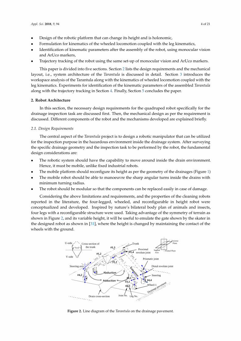
Considering the above limitations and requirements, and the properties of the cleaning robotsreported in the literature, the four-legged, wheeled, and reconfigurable in height robot wereconceptualized and developed. Inspired by nature’s bilateral body plan of animals and insects,four legs with a reconfigurable structure were used. Taking advantage of the symmetry of terrain asshown in Figure 2, and its variable height, it will be useful to emulate the gate shown by the skater inthe designed robot as shown in [31], where the height is changed by maintaining the contact of thewheels with the ground.

Trunk

Proximal

revolute joint

Prismatic joint

Distal revolute jointSteering axis

Abduction

Adduction

U-side

V-side

Cross-section of

the trunk

Wheel-1

Steering

Drain cross-section

#1,1

#2,1

#3,1

#4,1

Joint No. Leg No.

#4,2

#4,4

#1,2

#1,3

#1,4 Frontal Plane

Traverse

Plane

Sagittal

Axis

Figure 2. Line diagram of the Tarantula on the drainage pavement.

Appl. Sci. 2018, 9, 94 5 of 21

2.2. Mechanical Layout

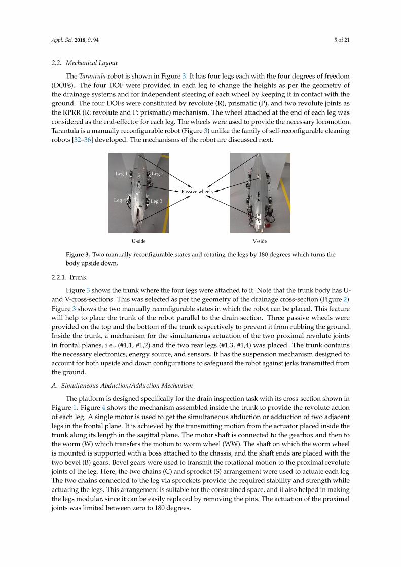
The Tarantula robot is shown in Figure 3. It has four legs each with the four degrees of freedom(DOFs). The four DOF were provided in each leg to change the heights as per the geometry ofthe drainage systems and for independent steering of each wheel by keeping it in contact with theground. The four DOFs were constituted by revolute (R), prismatic (P), and two revolute joints asthe RPRR (R: revolute and P: prismatic) mechanism. The wheel attached at the end of each leg wasconsidered as the end-effector for each leg. The wheels were used to provide the necessary locomotion.Tarantula is a manually reconfigurable robot (Figure 3) unlike the family of self-reconfigurable cleaningrobots [32–36] developed. The mechanisms of the robot are discussed next.

U-side V-side

Passive wheels

Leg 1 Leg 2

Leg 3Leg 4

Figure 3. Two manually reconfigurable states and rotating the legs by 180 degrees which turns thebody upside down.

2.2.1. Trunk

Figure 3 shows the trunk where the four legs were attached to it. Note that the trunk body has U-and V-cross-sections. This was selected as per the geometry of the drainage cross-section (Figure 2).Figure 3 shows the two manually reconfigurable states in which the robot can be placed. This featurewill help to place the trunk of the robot parallel to the drain section. Three passive wheels wereprovided on the top and the bottom of the trunk respectively to prevent it from rubbing the ground.Inside the trunk, a mechanism for the simultaneous actuation of the two proximal revolute jointsin frontal planes, i.e., (#1,1, #1,2) and the two rear legs (#1,3, #1,4) was placed. The trunk containsthe necessary electronics, energy source, and sensors. It has the suspension mechanism designed toaccount for both upside and down configurations to safeguard the robot against jerks transmitted fromthe ground.

A. Simultaneous Abduction/Adduction Mechanism

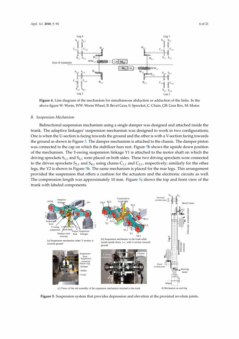
The platform is designed specifically for the drain inspection task with its cross-section shown inFigure 1. Figure 4 shows the mechanism assembled inside the trunk to provide the revolute actionof each leg. A single motor is used to get the simultaneous abduction or adduction of two adjacentlegs in the frontal plane. It is achieved by the transmitting motion from the actuator placed inside thetrunk along its length in the sagittal plane. The motor shaft is connected to the gearbox and then tothe worm (W) which transfers the motion to worm wheel (WW). The shaft on which the worm wheelis mounted is supported with a boss attached to the chassis, and the shaft ends are placed with thetwo bevel (B) gears. Bevel gears were used to transmit the rotational motion to the proximal revolutejoints of the leg. Here, the two chains (C) and sprocket (S) arrangement were used to actuate each leg.The two chains connected to the leg via sprockets provide the required stability and strength whileactuating the legs. This arrangement is suitable for the constrained space, and it also helped in makingthe legs modular, since it can be easily replaced by removing the pins. The actuation of the proximaljoints was limited between zero to 180 degrees.

Appl. Sci. 2018, 9, 94 6 of 21

W12

B2,1

B1,1S1,1 S2,1

S4,1 S3,1

S1,2

S4,2

WW12M12 GB12

S3,2

B2,3

B1,3

WW3,4 M34GB

C2,1C1,1

S2,2B1,2

B2,2

B1,4

B2,4

S2,3 S1,3

S3,3 S4,3

C2,3C1,3

S3,4 S4,4

S2,4 S1,4

C2,4C1,4

Leg 1

Leg 2Leg 3

Leg 4

Axis of symmetry

C1,2 C2,2

Figure 4. Line diagram of the mechanism for simultaneous abduction or adduction of the links. In theabove figure W: Worm, WW: Worm Wheel, B: Bevel Gear, S: Sprocket, C: Chain, GB: Gear Box, M: Motor.

B. Suspension Mechanism

Bidirectional suspension mechanism using a single damper was designed and attached inside thetrunk. The adaptive linkages’ suspension mechanism was designed to work in two configurations.One is when the U-section is facing towards the ground and the other is with a V-section facing towardsthe ground as shown in Figure 3. The damper mechanism is attached to the chassis. The damper pistonwas connected to the cap on which the stabilizer bars rest. Figure 5b shows the upside down positionof the mechanism. The Y-swing suspension linkage Y1 is attached to the motor shaft on which thedriving sprockets S1,1 and S2,1 were placed on both sides. These two driving sprockets were connectedto the driven sprockets S3,1 and S4,1 using chains C1,1 and C2,1, respectively; similarly for the otherlegs, the Y2 is shown in Figure 5b. The same mechanism is placed for the rear legs. This arrangementprovided the suspension that offers a cushion for the actuators and the electronic circuits as well.The compression length was approximately 10 mm. Figure 5c shows the top and front view of thetrunk with labeled components.

(a) Suspension mechanism when V-section is

towards ground

(b) Suspension mechanism to the trunk while

turned upside down, i.e., with U-section towards

ground

S1,2

S1,1

S4,1

S3,1

S2,1

B2,1

B1,1

S3,2S4,2

Connected to

trunk body

S2,2

Y1

Y2

Leg 1

Leg 2

Piston

RodDamper outer

housing

Y-swing

suspension

swingAdaptive

linkages

Suspension

linkages

slot

(c) Views of the sub assembly of the suspension mechanism attached to the trunk

Suspension

lever

Y-swing

suspension

C1,1

Leg 1

Leg 2

C2,1

C1,2

C2,2

Adaptive linkagesChassis

holders

Damper

Piston ring

Holder

Trunk

Suspension

leverSuspension

connector

S4,1 S3,1

Leg

1

Wheel

d) Mechanism on each leg

M1.1

M2.1

M3.1

Tel

esco

pic

exte

nsi

on

Steering

motor

Tel

esco

pic

act

uat

ion m

oto

r

Proximal

revolute joint

Distal

revolute joint

Bevel Gears

Connected to

trunk body

Figure 5. Suspension system that provides depression and elevation at the proximal revolute joints.

Appl. Sci. 2018, 9, 94 7 of 21

2.2.2. Telescopic Extension and Distal Revolute Joint

Figure 5d shows the arrangement of two pairs of the bevel gears with shafts used to actuate thescrew to get the telescopic action of the leg. Two motors were attached to the body of the telescopic link.The proximal motor, i.e., close to the trunk was used to actuate the telescopic screws, and the distalone was used to provide the revolute action parallel to the abduction/adduction motion. The distalrevolute joint was helpful in keeping the wheels in contact with the flat or inclined terrain (Figure 1).The kinematics of the mechanism is discussed in Section 3.

2.2.3. Steering and Wheel Suspension

The wheeled modular mechanism provides the mobility of the robot. Each of the four identicalwheel modules has the actuator for steering and the in-wheel motor for the propulsion. The steeringaction provided to each wheel gave the necessary four-wheel steering and four-wheel drive (FWSD).The FWSD is essential as the terrain of the drainage system can have sharp turns and curvatures.The control problem is non-trivial for the FWSD, but the requirement of moving the robot at relativelylow speed (1.8 to 2.5 Km h−1) using tethered communication and the simple controller is sufficient.The suspension system provided with the three compressed springs (s1, s2, and s3) attached to eachwheel is shown in Figure 6, which provides the required traction to the four wheels. It is also helpfulin safeguarding the motor and the micro-controller that is mounted on the wheel hub.

(a) Wheel suspension in CAD (b) Wheel suspension assembly

s1

Wheel holder

s2

s3

Motored Wheel

Figure 6. Wheel with suspensions.

2.2.4. Tarantula Electronics

Tarantula is controlled using the simple mechatronics system that uses the mechanical model ofthe vehicle and steering model to actuate the mechanism. The actuation and locomotion of the wheelswere achieved through the coordination between the micro-controller and actuators. An ArduinoAtmega2560 16-Bit micro-controller was mounted inside the trunk and was programmed to carry outthree major functions. Namely, (a) Control signal generation to the motor driver that controls themotor speed, (b) To receive the feedback of the motor positions, and (c) To obtain the user commandfrom the remote device or the computer. To reduce the number of wires connecting the motors to thecontroller, the controller area network (CAN) bus interface was used. Thin shielded cables were usedto connect the three Maxon motors (DCX22S, M11, M21, M31 as shown in Figure 5) with the connectorsfor controlling the motor modules, i.e., the telescopic action, the distal revolute joint and the steeringwith the CAN bus interface. The two motors placed inside the trunk for the simultaneous abductionand adduction, namely M12 and M34 (Figure 4) were connected with the micro-controller separately.

The 24-volt Lithium polymer batteries were kept inside the trunk body cover as the power source.The switching power supply fitted inside the servos allowed for running the servos efficiently atvoltages between 8 to 24 volts. These regulators allowed for using thinner wires between the modulesto supply sufficient power to the servos. The waterproof skateboard wheels with hub motors wereused. These were controlled with the speed and time period for the motors rotations which are definedby pulse-width modulation (PWM) signals from the micro-controller. The system architecture of a

Appl. Sci. 2018, 9, 94 8 of 21

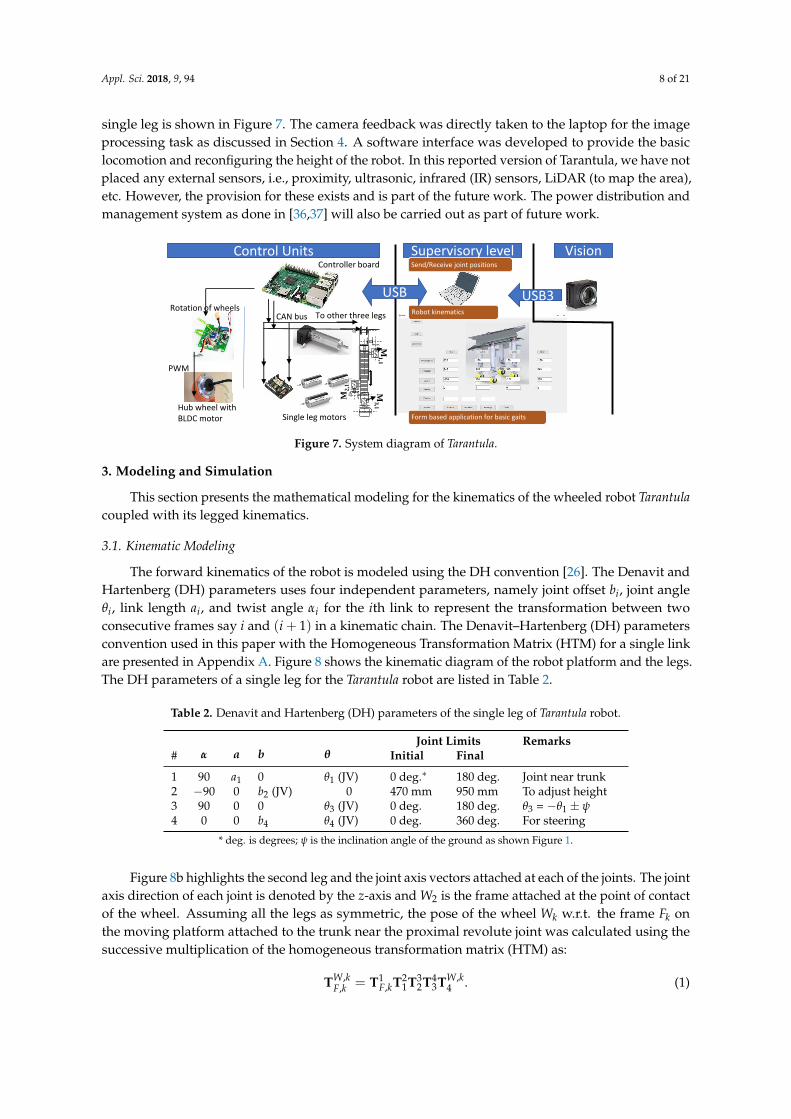
single leg is shown in Figure 7. The camera feedback was directly taken to the laptop for the imageprocessing task as discussed in Section 4. A software interface was developed to provide the basiclocomotion and reconfiguring the height of the robot. In this reported version of Tarantula, we have notplaced any external sensors, i.e., proximity, ultrasonic, infrared (IR) sensors, LiDAR (to map the area),etc. However, the provision for these exists and is part of the future work. The power distribution andmanagement system as done in [36,37] will also be carried out as part of future work.

Supervisory levelControl Units Vision

USB3

Send/Receive joint positions

Form based application for basic gaits

Robot kinematicsCAN bus

Single leg motorsHub wheel with BLDC motor

Rotation of wheels

PWM

Controller board

To other three legs

M1,1

M2,1

M3,1

USB

Figure 7. System diagram of Tarantula.

3. Modeling and Simulation

This section presents the mathematical modeling for the kinematics of the wheeled robot Tarantulacoupled with its legged kinematics.

3.1. Kinematic Modeling

The forward kinematics of the robot is modeled using the DH convention [26]. The Denavit andHartenberg (DH) parameters uses four independent parameters, namely joint offset bi, joint angleθi, link length ai, and twist angle αi for the ith link to represent the transformation between twoconsecutive frames say i and (i + 1) in a kinematic chain. The Denavit–Hartenberg (DH) parametersconvention used in this paper with the Homogeneous Transformation Matrix (HTM) for a single linkare presented in Appendix A. Figure 8 shows the kinematic diagram of the robot platform and the legs.The DH parameters of a single leg for the Tarantula robot are listed in Table 2.

Table 2. Denavit and Hartenberg (DH) parameters of the single leg of Tarantula robot.

α a b θJoint Limits Remarks

# Initial Final

1 90 a1 0 θ1 (JV) 0 deg.∗ 180 deg. Joint near trunk2 −90 0 b2 (JV) 0 470 mm 950 mm To adjust height3 90 0 0 θ3 (JV) 0 deg. 180 deg. θ3 = −θ1 ± ψ4 0 0 b4 θ4 (JV) 0 deg. 360 deg. For steering

* deg. is degrees; ψ is the inclination angle of the ground as shown Figure 1.

Figure 8b highlights the second leg and the joint axis vectors attached at each of the joints. The jointaxis direction of each joint is denoted by the z-axis and W2 is the frame attached at the point of contactof the wheel. Assuming all the legs as symmetric, the pose of the wheel Wk w.r.t. the frame Fk onthe moving platform attached to the trunk near the proximal revolute joint was calculated using thesuccessive multiplication of the homogeneous transformation matrix (HTM) as:

TW,kF,k = T1

F,kT21T3

2T43TW,k

4 . (1)

Appl. Sci. 2018, 9, 94 9 of 21

The subscript k is for the four legs of the quadruped, i.e., k = 1, · · · , 4. Here, it is assumed thatthe geometry of the legs are identical, and hence the DH parameters remain the same for the four legs.After substituting the values of DH parameters and post multiplying the HTM, the position of thewheels in the frame attached to the proximal revolute joint is:

TW,kF,k =

Cθ12,kCθ4,k −Cθ12,kSθ4,k Sθ13,k b4,kSθ13.k + a1,kCθ1,k + b2Sθ1,kSθ12,kCθ4,k −Sθ12,kSθ4,k 0 0

Sθ4,k Cθ4,k 0 b4,kCθ13.k − a1,kSθ1,k + b2Cθ1,k0 0 0 1

. (2)

The above expression written in the fixed frame attached to the trunk of the robot byprep-multiplying it with the HTM (coordinates and orientation of the frame shown in Figure 8) is:

TW,kT = TF,k

T TW,kF,k . (3)

The first three elements in the fourth column of Equation (2) give the position of the wheel,i.e., [xw,k, yw,k, zw,k]

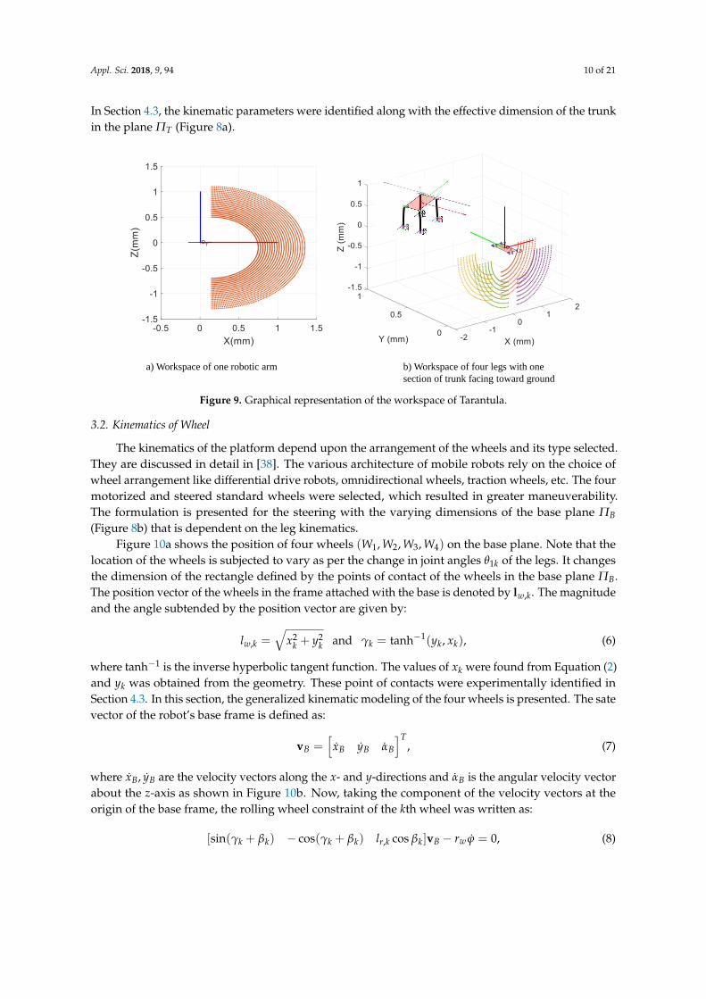
T . The y-coordinates are explicitly shown in Figure 8, and it does not vary w.r.t.,the frame attached with the trunk. The two-dimensional graphical representation of the workspaceof a single leg is depicted in Figure 9a and, with four legs considering the constraint in Equation (5),is shown in Figure 9b.

Leg 1

Leg 2

Leg 3

Leg 4

{ }T

1{ }F

2{ }F

3{ }F4{ }F

, ,02 2

b bd l

{ }B

bd

td

bl

tl{ }T

a) Frames attached with the trunk and legs b) Frames attached with the leg

𝜃1,3

𝜃1,2

𝜃1,4

𝜃1,4

𝜃3,2

𝜃4,2

{ }IInertial

Frame

𝑧 𝑡

, ,02 2

t td l

,2FZ

1,2Z

2,2Z

3,2Z

2{ }W

3{ }W

1{ }W

4{ }W 4,2Z 𝑏4

, ,02 2

t td l

, ,02 2

t td l

, ,02 2

t td l

T

B

{ }F

Figure 8. The inertial frame {I}, body fixed frame {T} at the trunk, base frame {B} at the center ofthe contact point of four wheels with the ground and the DH frames attached with leg 2 havingRPRR joints.

The kinematic constraint or dependencies that are utilized for the simultaneous abduction andadduction of all four legs as per the actuation mechanism in the Trunk is written as:

θ1,1 = θ1,4 = −θ1,2 = −θ1,3. (4)

Another constraint to maintain the contact of the four wheels with the inclined surface can bewritten as:

θ3,1 = −θ1,1 ± ψ, θ3,2 = θ1,2 ± ψ, θ3,3 = −θ1,3 ± ψ and θ3,4 = −θ1,4 ± ψ, (5)

where ψ is the angle of inclination of the pavement as shown in Figure 1. The above constraintsfor any flat surface perpendicular to the direction of gravity were obtained by substituting ψ = 0.

Appl. Sci. 2018, 9, 94 10 of 21

In Section 4.3, the kinematic parameters were identified along with the effective dimension of the trunkin the plane ΠT (Figure 8a).

a) Workspace of one robotic arm b) Workspace of four legs with one

section of trunk facing toward ground

Figure 9. Graphical representation of the workspace of Tarantula.

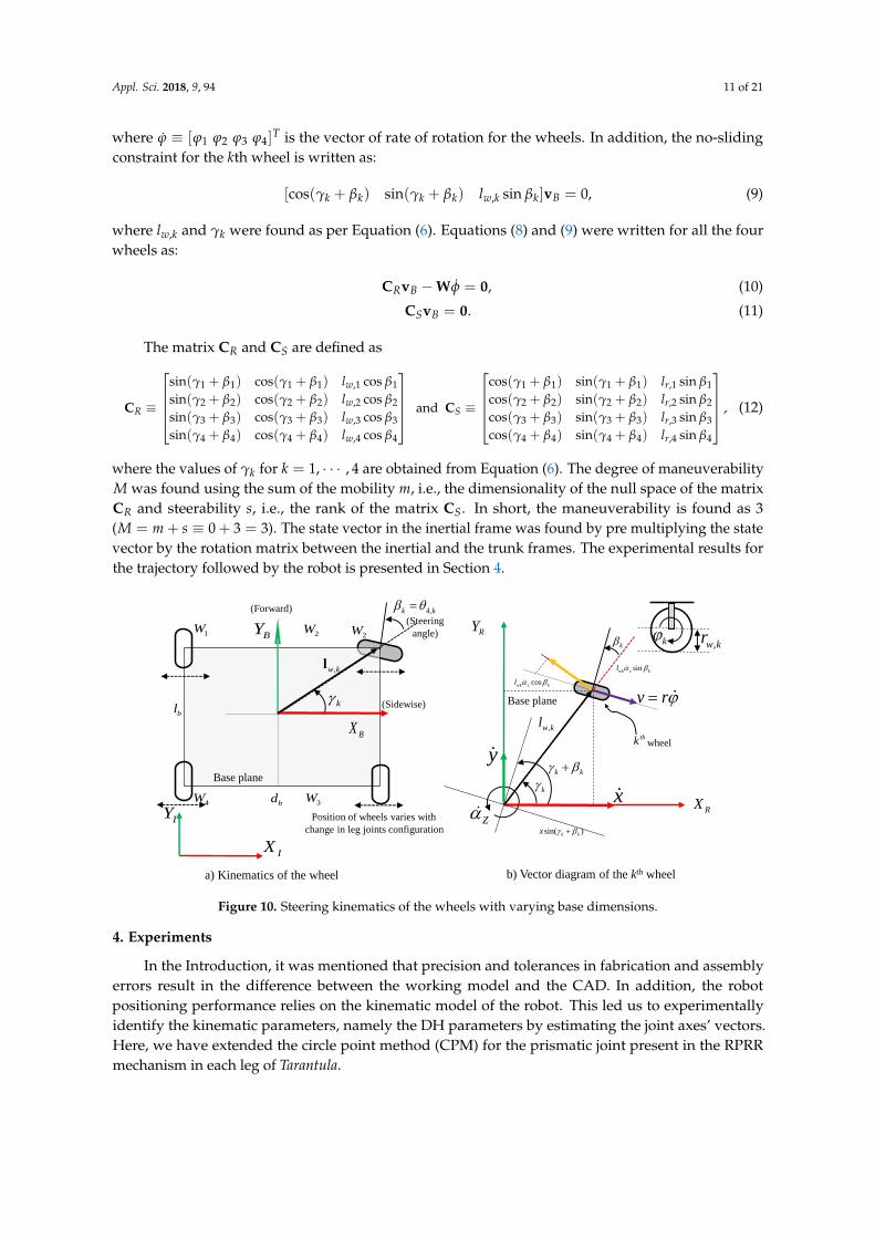
3.2. Kinematics of Wheel

The kinematics of the platform depend upon the arrangement of the wheels and its type selected.They are discussed in detail in [38]. The various architecture of mobile robots rely on the choice ofwheel arrangement like differential drive robots, omnidirectional wheels, traction wheels, etc. The fourmotorized and steered standard wheels were selected, which resulted in greater maneuverability.The formulation is presented for the steering with the varying dimensions of the base plane ΠB(Figure 8b) that is dependent on the leg kinematics.

Figure 10a shows the position of four wheels (W1, W2, W3, W4) on the base plane. Note that thelocation of the wheels is subjected to vary as per the change in joint angles θ1k of the legs. It changesthe dimension of the rectangle defined by the points of contact of the wheels in the base plane ΠB.The position vector of the wheels in the frame attached with the base is denoted by lw,k. The magnitudeand the angle subtended by the position vector are given by:

lw,k =√

x2k + y2

k and γk = tanh−1(yk, xk), (6)

where tanh−1 is the inverse hyperbolic tangent function. The values of xk were found from Equation (2)and yk was obtained from the geometry. These point of contacts were experimentally identified inSection 4.3. In this section, the generalized kinematic modeling of the four wheels is presented. The satevector of the robot’s base frame is defined as:

vB =[

xB yB αB

]T, (7)

where xB, yB are the velocity vectors along the x- and y-directions and αB is the angular velocity vectorabout the z-axis as shown in Figure 10b. Now, taking the component of the velocity vectors at theorigin of the base frame, the rolling wheel constraint of the kth wheel was written as:

[sin(γk + βk) − cos(γk + βk) lr,k cos βk]vB − rw ϕ = 0, (8)

Appl. Sci. 2018, 9, 94 11 of 21

where ϕ ≡ [ϕ1 ϕ2 ϕ3 ϕ4]T is the vector of rate of rotation for the wheels. In addition, the no-sliding

constraint for the kth wheel is written as:

[cos(γk + βk) sin(γk + βk) lw,k sin βk]vB = 0, (9)

where lw,k and γk were found as per Equation (6). Equations (8) and (9) were written for all the fourwheels as:

CRvB −Wφ = 0, (10)

CSvB = 0. (11)

The matrix CR and CS are defined as

CR ≡

sin(γ1 + β1) cos(γ1 + β1) lw,1 cos β1

sin(γ2 + β2) cos(γ2 + β2) lw,2 cos β2

sin(γ3 + β3) cos(γ3 + β3) lw,3 cos β3

sin(γ4 + β4) cos(γ4 + β4) lw,4 cos β4

and CS ≡

cos(γ1 + β1) sin(γ1 + β1) lr,1 sin β1

cos(γ2 + β2) sin(γ2 + β2) lr,2 sin β2

cos(γ3 + β3) sin(γ3 + β3) lr,3 sin β3

cos(γ4 + β4) sin(γ4 + β4) lr,4 sin β4

, (12)

where the values of γk for k = 1, · · · , 4 are obtained from Equation (6). The degree of maneuverabilityM was found using the sum of the mobility m, i.e., the dimensionality of the null space of the matrixCR and steerability s, i.e., the rank of the matrix CS. In short, the maneuverability is found as 3(M = m + s ≡ 0 + 3 = 3). The state vector in the inertial frame was found by pre multiplying the statevector by the rotation matrix between the inertial and the trunk frames. The experimental results forthe trajectory followed by the robot is presented in Section 4.

4,k k =

k

bd

bl

3W

Base plane

2W

4W

1W

(Forward)

(Sidewise)

a) Kinematics of the wheel

IY

IX

BX

BY2W

(Steering

angle)

Position of wheels varies with

change in leg joints configuration

,w krkRY

RX

k

x

y

Z

k

v r=Base plane

,w kl

wheel thk

k k +

b) Vector diagram of the kth wheel

,w kl

coswk z kl

sinwk z kl

sin( )k kx +

Figure 10. Steering kinematics of the wheels with varying base dimensions.

4. Experiments

In the Introduction, it was mentioned that precision and tolerances in fabrication and assemblyerrors result in the difference between the working model and the CAD. In addition, the robotpositioning performance relies on the kinematic model of the robot. This led us to experimentallyidentify the kinematic parameters, namely the DH parameters by estimating the joint axes’ vectors.Here, we have extended the circle point method (CPM) for the prismatic joint present in the RPRRmechanism in each leg of Tarantula.

Appl. Sci. 2018, 9, 94 12 of 21

4.1. Setup

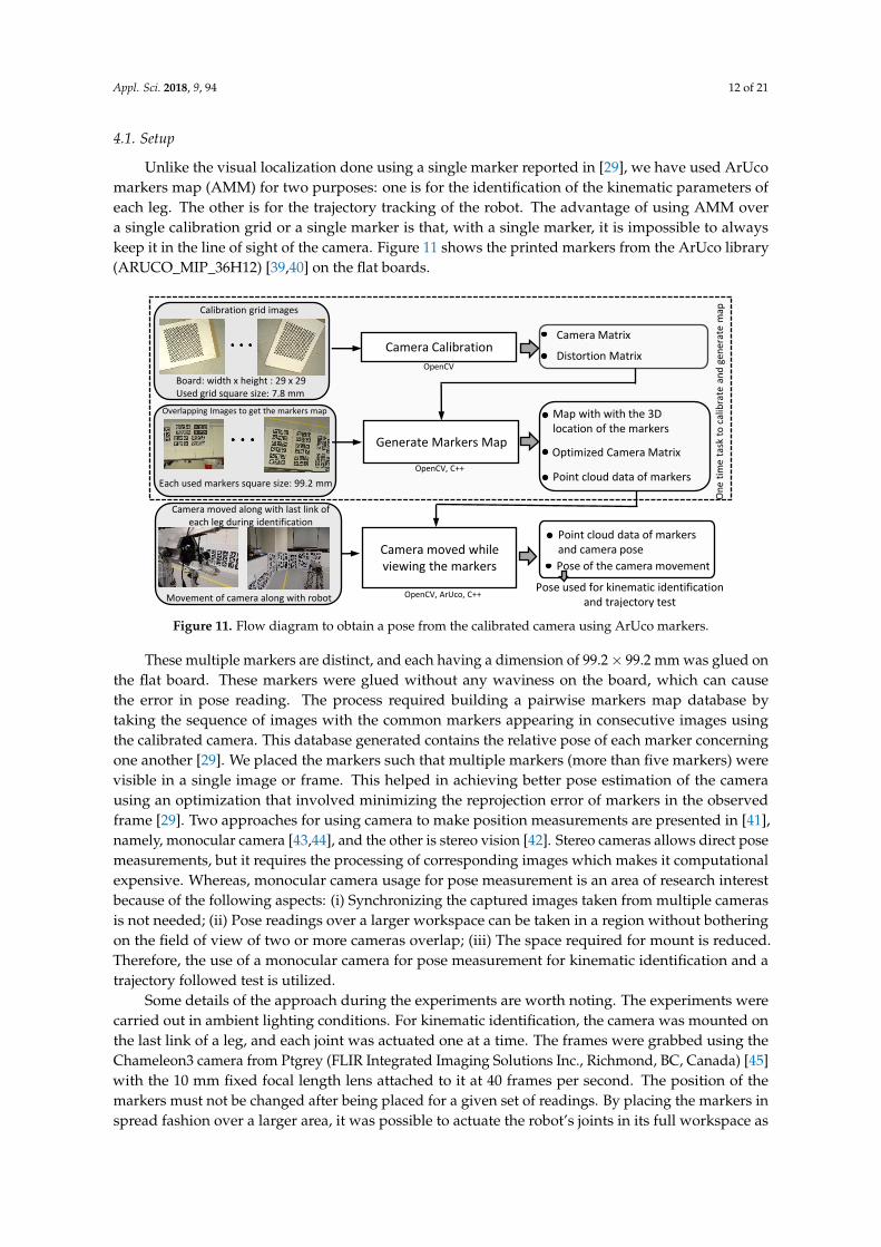
Unlike the visual localization done using a single marker reported in [29], we have used ArUcomarkers map (AMM) for two purposes: one is for the identification of the kinematic parameters ofeach leg. The other is for the trajectory tracking of the robot. The advantage of using AMM overa single calibration grid or a single marker is that, with a single marker, it is impossible to alwayskeep it in the line of sight of the camera. Figure 11 shows the printed markers from the ArUco library(ARUCO_MIP_36H12) [39,40] on the flat boards.

Camera Calibration

Generate Markers Map

Camera moved while viewing the markers

Camera Matrix

Board: width x height : 29 x 29Used grid square size: 7.8 mm

Distortion Matrix

Each used markers square size: 99.2 mm

Map with with the 3D location of the markers

Optimized Camera Matrix

Point cloud data of markers

Point cloud data of markers and camera pose

Pose of the camera movement

Overlapping Images to get the markers map

Calibration grid images

Movement of camera along with robot OpenCV, ArUco, C++

OpenCV, C++

OpenCV

On

e ti

me

task

to

cal

ibra

te a

nd

gen

erat

e m

ap

Camera moved along with last link of each leg during identification

Pose used for kinematic identification and trajectory test

Figure 11. Flow diagram to obtain a pose from the calibrated camera using ArUco markers.

These multiple markers are distinct, and each having a dimension of 99.2× 99.2 mm was glued onthe flat board. These markers were glued without any waviness on the board, which can causethe error in pose reading. The process required building a pairwise markers map database bytaking the sequence of images with the common markers appearing in consecutive images usingthe calibrated camera. This database generated contains the relative pose of each marker concerningone another [29]. We placed the markers such that multiple markers (more than five markers) werevisible in a single image or frame. This helped in achieving better pose estimation of the camerausing an optimization that involved minimizing the reprojection error of markers in the observedframe [29]. Two approaches for using camera to make position measurements are presented in [41],namely, monocular camera [43,44], and the other is stereo vision [42]. Stereo cameras allows direct posemeasurements, but it requires the processing of corresponding images which makes it computationalexpensive. Whereas, monocular camera usage for pose measurement is an area of research interestbecause of the following aspects: (i) Synchronizing the captured images taken from multiple camerasis not needed; (ii) Pose readings over a larger workspace can be taken in a region without botheringon the field of view of two or more cameras overlap; (iii) The space required for mount is reduced.Therefore, the use of a monocular camera for pose measurement for kinematic identification and atrajectory followed test is utilized.

Some details of the approach during the experiments are worth noting. The experiments werecarried out in ambient lighting conditions. For kinematic identification, the camera was mounted onthe last link of a leg, and each joint was actuated one at a time. The frames were grabbed using theChameleon3 camera from Ptgrey (FLIR Integrated Imaging Solutions Inc., Richmond, BC, Canada) [45]with the 10 mm fixed focal length lens attached to it at 40 frames per second. The position of themarkers must not be changed after being placed for a given set of readings. By placing the markers inspread fashion over a larger area, it was possible to actuate the robot’s joints in its full workspace as

Appl. Sci. 2018, 9, 94 13 of 21

shown in Figure 9b. The frame was grabbed using the camera, and the pose was obtained using theflow diagram presented in Figure 11. The evaluation of the measurement approach proposed here ispresented next.

4.2. Measurement Performance

Evaluation of the proposed measurement technique was done by mounting the camera on theKUKA KR6 R900 robot that has the measurement performance of 0.03 mm [30]. The robot’s end-effectorwith the camera mounted was made to move in the x-, y- and z-axis directions of the robots worldframe. The initial distance of the camera from the markers was 3.4 m. The initial and final coordinates ofthe robot were recorded from the teach-pendent (Figure 12a) for movement along each axes. The poseobtained from the camera is plotted in Figure 12b. The measured angle between the given motionabout each axis is shown in Figure 12c. Assuming the readings from the robot as the ground truth,the trajectory of the robot end-effector is compared to the one obtained using the monocular camera.Table 3 lists the ideal and the measured distances using the markers. It is observed that variationalong the y-direction is highest and in this case, the camera was moving towards the markers, i.e.,perpendicular to the plane of the markers. In the rest two of the directions, the variations are within3 mm. Hence the movement in a plane along the markers is closer to the ideal than the depth one.

a) ArUco markers and KUKA KR6 R900

robot mounted with camera b) Pose of the camera moved along the robot’s X-,

Y-, and Z- axis with AB and EF making cross

Markers

Camera

+X

+Y

+Z

Teach Pendent

c) Robot pose and measured angles

Y(m)

89.8489.89

90.07

AB

C

D

E

F

A

B

C

D

E

F

Figure 12. Evaluation of measurements using the ArUco markers and monocular camera.

Table 3. Evaluation of measurement performance using monocular camera and ArUco markers.

X : AB (m) Y : CD (m) Z : EF (m) ](AB, CD) ](CD, EF) ](EF, AB)

Ideal (Robot) 0.400 0.7776 0.7467 90 90 90Measured (Markers) 0.3987 0.7235 0.7494 89.89 89.84 90.07

X :, Y :, Z : means x-, y- and z-directions in robots world frame, ]: Angles are in degrees.

Appl. Sci. 2018, 9, 94 14 of 21

4.3. Identification of Kinematic Parameters of Tarantula

After the assembly of Tarantula, the identification of the proximal revolute joint positions andkinematic parameters of each leg is essential. The mathematical analysis of the measured data to obtainthe joint axis vectors (JAVs) presented elsewhere [25] is discussed in short for brevity along with itsextension for the prismatic joints. The points traced by the end-effector, i.e., the three-dimensional (3D)coordinates (xi ≡ [xi, yi, zi]

T) were logged and stacked in a matrix A (Equation (13)). The mean of thelogged pose data points was subtracted from the elements of A which resulted in the transformed setof points in a matrix B whose mean is zero. Matrices of three-dimensional data points, D and D areshown below:

A = [x1 x2 · · · xm]T

; A = [(x1 − x) (x2 − x) · · · (xm − x)]T

, (13)

where x ≡ [x y z]T = 1m [∑ xi ∑ yi ∑ zi]

T , and m being the number of measurements.Applying singular value decomposition (SVD) [46] on matrix A, two square orthogonal matricesU and V and a rectangular matrix D were obtained as:

A = Vm×mDm×3U3×m. (14)

The orthogonal columns corresponding to the singular values (SVs) are listed in the column ofmatrix U ≡ [u1 u2 u3]. The direction of the joint axis represented by the unit vector n in Figure 13a forrevolute and Figure 13b for prismatic is given as:

n ≡ u3 for rotary joints, (15a)

n ≡ u1 for linearactuating joints. (15b)

The above equations gave the joint axis vector direction. For a point on the JAV, the center ofcircle c, i.e., the center of rotation for revolute joint was obtained using circle fitting method presentedin [25], where c ≡ c1u1 + c2u2 + x, c1 and c2 are the center of fitted circle in the plane spanned byvectors u1 and u2. For prismatic joint the mean of the traced point, i.e., c ≡ x was taken as the point onthe JAV of prismatic joints. The plane of link movement Π can be defined as:

Π ≡[

n−nT x

]. (16)

Center

(x1, y1, z1) 2v

1u

(a) Center and orthogonal directions

for revolute joints

(b) Singular values and normal direction for

prismatic joints

plane Π

n

X

ZY

plane

Π Ci

Measurement frame

c

Zi(xm, ym, zm)

1u

2u3u

2u3u

Mean of points logged with

prismatic joint

(cx, cy, cz)

(x1, y1, z1)

n

X

Z

Y

c

Figure 13. Position data points on the circle and the line obtained with the revolute and prismatic jointactuation respectively with its singular value direction.

Appl. Sci. 2018, 9, 94 15 of 21

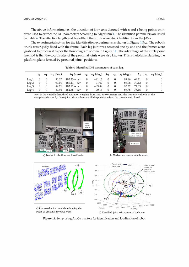
The above information, i.e., the direction of joint axis denoted with n and c being points on it,were used to extract the DH parameters according to Algorithm 1. The identified parameters are listedin Table 4. The effective length and breadth of the trunk were also identified from the JAVs.

The experimental set-up for the identification experiments is shown in Figure 14b,c. The robot’strunk was rigidly fixed with the frame. Each leg joint was actuated one by one and the frames weregrabbed to process it as per the flow diagram shown in Figure 11. The advantage of the circle pointmethod is that the coordinates of the proximal joints were also known. This is helpful in defining theplatform plane formed by proximal joints’ positions.

Table 4. Identified DH parameters of each leg.

b1 a1 α1 (deg.) b2 (mm) a2 α2 (deg.) b3 a3 α3 (deg.) b4 a4 α4 (deg.)

Leg 1 0 0 90.17 485.23 + var 0 −91.13 0 0 89.86 69.21 0 0Leg 2 0 0 90.01 480.13 + var 0 −91.07 0 0 89.06 70.12 0 0Leg 3 0 0 89.71 482.72 + var 0 −89.89 0 0 90.32 72.35 0 0Leg 4 0 0 89.96 482.36 + var 0 −90.14 0 0 89.78 78.16 0 0

var: is the variable length of actuation varying from zero to 0.6 meters and the numeric value is at thecompressed state. b4: these joint offset values are till the position where the camera was placed.

a) Testbed for the kinematic identification

J1

J2

J3

J4Camera

ArUco markers

glued on flat boards

c) Processed point cloud data showing the

poses of proximal revolute joints

Pose data

Leg 1

MarkersLeg 2

Leg 3Leg 4

d) Identified joint axis vectors of each joint

Leg 1

Leg 2

Leg 3

Leg 4

JAVFitted circlePlane of trunk

formed by

proximal

revolute joints

Fitted line

b) Markers and camera with the joints

Leg 1Leg 4

Leg 2Leg 3

Frames

acquired

in laptop

J3,1

J2,1

J4,1

Figure 14. Setup using AruCo markers for identification and localization of robot.

Appl. Sci. 2018, 9, 94 16 of 21

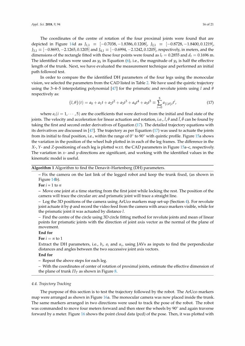
The coordinates of the centre of rotation of the four proximal joints were found that aredepicted in Figure 14d as J1,1 ≡ [−0.7038,−1.8386, 0.1208], J2,1 ≡ [−0.8728,−1.8400, 0.1219],J3,1 ≡ [−0.8693,−2.1265, 0.1205] and J4,1 ≡ [−0.6994,−2.1242, 0.1205], respectively, in meters, and thedimensions of the rectangle fitted with these four points were found as lt = 0.2855 and dt = 0.1696 m.The identified values were used as yk in Equation (6), i.e., the magnitude of yk is half the effectivelength of the trunk. Next, we have evaluated the measurement technique and performed an initialpath followed test.

In order to compare the the identified DH parameters of the four legs using the monocularvision, we selected the parameters from the CAD listed in Table 2. We have used the quintic trajectoryusing the 3–4–5 interpolating polynomial [47] for the prismatic and revolute joints using l and θ

respectively as:

{l, θ}(t) = a0 + a1t + a2t2 + a3t3 + a4t4 + a5t5 ≡5

∑i=0

a{l,θ}iti, (17)

where ai(i = 1, · · · , 5) are the coefficients that were derived from the initial and final state of thejoints. The velocity and acceleration for linear actuation and rotation, i.e., l, θ and l, θ can be found bytaking the first and second order derivatives of Equation (17). The detailed trajectory equations withits derivatives are discussed in [47]. The trajectory as per Equation (17) was used to actuate the jointsfrom its initial to final position, i.e., within the range of 0◦ to 90◦ with quintic profile. Figure 15a showsthe variation in the position of the wheel hub plotted in in each of the leg frames. The difference in theX-, Y- and Z-positioning of each leg is plotted w.r.t. the CAD parameters in Figure 15a–c, respectively.The variation in x- and y-directions are significant, and working with the identified values in thekinematic model is useful.

Algorithm 1 Algorithm to find the Denavit–Hartenberg (DH) parameters.

– Fix the camera on the last link of the legged robot and keep the trunk fixed, (as shown inFigure 14b).For i = 1 to n– Move one joint at a time starting from the first joint while locking the rest. The position of thecamera will trace the circular arc and prismatic joint will trace a straight line.– Log the 3D positions of the camera using ArUco markers map set-up (Section 4). For revolutejoint actuate it by φ and record the video feed from the camera with aruco markers visible, while forthe prismatic joint it was actuated by distance l.– Find the centre of the circle using 3D circle fitting method for revolute joints and mean of linearpoints for prismatic joints with the direction of joint axis vector as the normal of the plane ofmovement.End forFor i = n to 1Extract the DH parameters, i.e., bi, ai and αi, using JAVs as inputs to find the perpendiculardistances and angles between the two successive joint axis vectors.End for– Repeat the above steps for each leg.– With the coordinates of center of rotation of proximal joints, estimate the effective dimension ofthe plane of trunk ΠT as shown in Figure 8.

4.4. Trajectory Tracking

The purpose of this section is to test the trajectory followed by the robot. The ArUco markersmap were arranged as shown in Figure 16a. The monocular camera was now placed inside the trunk.The same markers arranged in two directions were used to track the pose of the robot. The robotwas commanded to move four meters forward and then steer the wheels by 90◦ and again traverseforward by a meter. Figure 16 shows the point cloud data (pcd) of the pose. Then, it was plotted with

Appl. Sci. 2018, 9, 94 17 of 21

the coordinate frame attached at one of the markers. The trajectory followed obtained after fitting theline is shown in Figure 16b with the angle of turn obtained as 87.8 degrees. Note that, in this case,the frames were recorded after every 100 milliseconds for the total trajectory time of 2.3 s. The distancetraversed is shown in Figure 16c. The difference in the desired and the obtained trajectory is mainlydue to the friction and uncertainties in the model. The limitations of this approach are the measuringvariations in the pose that can be ±3 mm at a distance of 4–5 m of the camera from the markers andalso the lighting conditions affect the detection of the markers.

a) Comparison of the position of wheel hub of each

leg found using identified parameters w.r.t., the CADb) Difference in X-positioning

X

YZ

Plotted position

d) Difference in Z-positioning c) Difference in Y-positioning

Dif

fere

nce

(m

m)

L,3

L,3L,3

CAD

Figure 15. Comparison of the positioning of each leg w.r.t. the CAD.

(b) Processed point cloud data showing the trajectory

followed by the robot

a) ArUco marker maps arranged for trajectory test

(c) Path traced by the robot with the sharp turn

Figure 16. Experimental setup and the trajectory traced by the robot.

Appl. Sci. 2018, 9, 94 18 of 21

5. Conclusions and Future Works

In this paper, Tarantula’s design, modeling, and its kinematic parameters identification arepresented. The robot was designed for the specific geometry of the drains. The designed manipulatoris modular and can adjust its height as per the environment. The simultaneous abduction or adductionof the two legs in a frontal plane was provided using the chain sprocket mechanisms connectedusing bevel gears arrangement with a single motor. A specially designed bi-directional suspensionmechanism was fixed inside the trunk as a shock absorber. The limitation of the chain sprocket is thatit imparts the rotational play because of slacking.

To the best of the author’s knowledge, this is the first attempt to estimate the kinematic parametersof the assembled robot with four leg using monocular camera mounted on the assembled Tarantula.This method also identified the effective dimension of the trunk where the proximal revolute jointswere connected. The limitations of the monocular vision and fiducial markers to obtain the pose isthat the camera must view the markers in the generated map. We also performed the experiments toevaluate the trajectory tracked by Tarantula using a similar set-up. Overall, the contributions of thispaper are listed below:

• Design of the modular robot Tarantula with the ability to reconfigure its height, mainly forinspecting the drains,

• A mechanism designed for the simultaneous abduction/adduction of legs,• A methodology to identify the kinematic parameters using ArUco markers and monocular vision

for the assembled mobile robot with legs. First, using the calibrated camera, poses of ArUcomarkers are reconstructed in 3D space. Second, by moving each joint and capturing images, a setof the tracked pose is determined. Then, the DH parameters were evaluated.

The domains set for future research work will mainly focus on: design optimization of the legs toreduce the total weight. Since the design is modular, the newly designed legs can be easily attached tothe existing trunk. The second focus will be to mount the Light Detection and Ranging (LiDAR) sensornear the trunk opening of Tarantula to map the drains.

Author Contributions: A.A.H. and M.R.E. conceived and designed the experiments;the experiments; A.A.H.and K.E. performed the experiments; A.A.H. and K.E. analyzed the data; K.E., A.A.H. and M.S.T. contributedreagents/materials/analysis tools; A.A.H., K.E., M.S.T. and M.R.E., wrote the paper.

Funding: This work is financially supported by the National Robotics R&D Program Office, Singapore, under theGrant No. RGAST1702 to Singapore University of Technology and Design (SUTD) which are greatly acknowledgedto conduct this research.

Conflicts of Interest: The authors declare no conflict of interest.

Appendix A. DH Parameters Notation Used [48]

In this appendix, the definitions of Denavit–Hartenberg (DH) parameters are presented forcompleteness of the paper. Note that four parameters, namely, bi, θi, ai and αi, relate the transformationbetween two frames i and i + 1 which are rigidly attached to two consecutive links #(i− 1) and #(i),respectively, as shown in Figure A1. Their notations and descriptions are summarized in Table A1.

#( 1)i #( )i

Frame

Frame#( 1)i

#( )i

Figure A1. Links and DH parameters.

Appl. Sci. 2018, 9, 94 19 of 21

The resulting coordinate transformation between the frames connected to link i and i + 1 as:

Ti+1i = Tbi

Tθi Tai Tαi (A1a)

=

1 0 0 00 1 0 00 0 1 bi0 0 0 1

Cθi −Sθi 0 0Sθi Cθi 0 00 0 1 00 0 0 1

1 0 0 ai0 1 0 00 0 1 00 0 0 1

1 0 0 00 Cαi −Sαi 00 Sαi Cαi 00 0 0 1

(A1b)

=

Cθi −SθiCαi SθiSαi aiCθiSθi CθiCαi −CθiSαi aiSθi0 Sαi Cαi bi0 0 0 1

. (A1c)

Table A1. Notations and descriptions of the DH parameters [26].

Parameters (Name) Description *

bi (Joint offset) Xi⊥,distance−−−−−−→

@ZiXi+1

θi (Joint angle) Xiccw, rotation−−−−−−−→

@ZiXi+1

ai (Link length) Zi⊥,distance−−−−−−→

@Xi+1Zi+1

αi (Twist angle) Ziccw, rotation−−−−−−−→

@Xi+1Zi+1

In the table read symbol −→ as “and”, ⊥ as “perpendicular”, @ as “along”and ccw as “counter clockwise”.

References

1. Zhang, S.X.; Pramanik, N.; Buurman, J. Exploring an innovative design for sustainable urban watermanagement and energy conservation. Int. J. Sustain. Dev. World Ecol. 2013, 20, 442–454. [CrossRef]

2. Kirkham, R.; Kearney, P.D.; Rogers, K.J.; Mashford, J. PIRAT—A system for quantitative sewer pipeassessment. Int. J. Robot. Res. 2000, 19, 1033–1053. [CrossRef]

3. Bradbeer, R. The Pearl Rover Underwater Inspection Robot. In Mechatronics and Machine Vision;Billingsley, J., Ed.; Research Studies Press: Baldock, UK, 2000; pp. 255–262.

4. Truong-Thinh, N.; Ngoc-Phuong, N.; Phuoc-Tho, T. A study of pipe-cleaning and inspection robot.In Proceedings of the International Conference on Robotics and Biomimetics (ROBIO), Karon Beach, Phuket,Thailand, 7–11 December 2011; pp. 2593–2598.

5. Kuntze, H.; Schmidt, D.; Haffner, H.; Loh, M. KARO-A flexible robot for smart sensor-based sewer inspection.In Proceedings of the No Dig’95, Dresden, Germany, 19–22 September 1995; pp. 367–374.

6. Nassiraei, A.A.; Kawamura, Y.; Ahrary, A.; Mikuriya, Y.; Ishii, K. Concept and design of a fully autonomoussewer pipe inspection mobile robot KANTARO. In Proceedings of the International Conference on Roboticsand Automation, Roma, Italy, 10–14 April 2007; pp. 136–143.

7. Kirchner, F.; Hertzberg, J. A prototype study of an autonomous robot platform for sewerage systemmaintenance. Auton. Robots 1997, 4, 319–331. [CrossRef]

8. Streich, H.; Adria, O. Software approach for the autonomous inspection robot MAKRO. In Proceedings ofthe International Conference on Robotics and Automation, New Orleans, LA, USA, 26 April–1 May 2004;Volume 4, pp. 3411–3416.

9. Baghani, A.; Ahmadabadi, M.N.; Harati, A. Kinematics modeling of a wheel-based pole climbingrobot (UT-PCR). In Proceedings of the 2005 IEEE International Conference on Robotics and Automation(ICRA 2005), Barcelona, Spain, 18–22 April 2005; pp. 2099–2104.

10. Ratanghayra, P.R.; Hayat, A.A.; Saha, S.K. Design and Analysis of Spring-Based Rope Climbing Robot.In Machines, Mechanism and Robotics; Springer: Berlin, Germany, 2019; pp. 453–462.

Appl. Sci. 2018, 9, 94 20 of 21

11. Fuchida, M.; Pathmakumar, T.; Mohan, R.E.; Tan, N.; Nakamura, A. Vision-based perception andclassification of mosquitoes using support vector machine. Appl. Sci. 2017, 7, 51. [CrossRef]

12. Raibert, M.H. Legged Robots That Balance; MIT Press: Cambridge, MA, USA, 1986.13. Berns, K.; Ilg, W.; Deck, M.; Albiez, J.; Dillmann, R. Mechanical construction and computer architecture of

the four-legged walking machine BISAM. IEEE/ASME Trans. Mechatron. 1999, 4, 32–38. [CrossRef]14. Ridderstrom, C.; Ingvast, J. Quadruped posture control based on simple force distribution-a notion and

a trial. In Proceedings of the International Conference on Intelligent Robots and Systems, Maui, HI, USA,29 October–3 November 2001; Volume 4, pp. 2326–2331.

15. Hirose, S.; Kato, K. Study on quadruped walking robot in Tokyo Institute of Technology-past, present andfuture. In Proceedings of the International Conference on Robotics and Automation, San Francisco, CA,USA, 24–28 April 2000; Volume 1, pp. 414–419.

16. Kitano, S.; Hirose, S.; Endo, G.; Fukushima, E.F. Development of lightweight sprawling-type quadrupedrobot titan-xiii and its dynamic walking. In Proceedings of the International Conference on IntelligentRobots and Systems (IROS), Tokyo, Japan, 3–7 November 2013; pp. 6025–6030.

17. Arikawa, K.; Hirose, S. Development of quadruped walking robot TITAN-VIII. In Proceedings of theIEEE/RSJ International Conference on Intelligent Robots and Systems (IROS 96), Osaka, Japan, 8 November1996; Volume 1, pp. 208–214.

18. De Santos, P.G.; Garcia, E.; Estremera, J. Quadrupedal Locomotion: An Introduction to the Control of Four-LeggedRobots; Springer Science & Business Media: Berlin, Germany, 2007.

19. Montes, H.; Armada, M. Force control strategies in hydraulically actuated legged robots. Int. J. Adv.Robot. Syst. 2016, 13, 50. [CrossRef]

20. Li, T.; Ma, S.; Li, B.; Wang, M.; Li, Z.; Wang, Y. Development of an in-pipe robot with differential screwangles for curved pipes and vertical straight pipes. J. Mech. Robot. 2017, 9, 051014. [CrossRef]

21. Sharf, I. Dynamic Locomotion with a Wheeled-Legged Quadruped Robot. In Brain, Body and Machine;Springer: Berlin, Germany, 2010; pp. 299–310.

22. Barker, L.K. Vector-Algebra Approach to Extract Denavit–Hartenberg Parameters of Assembled Robot Arms; NASALangley Research Center: Hampton, VA, USA, 1983.

23. Hollerbach, J.M.; Wampler, C.W. The calibration index and taxonomy for robot kinematic calibrationmethods. Int. J. Robot. Res. 1996, 15, 573–591. [CrossRef]

24. De Santos, P.G.; Jiménez, M.A.; Armada, M.A. Improving the motion of walking machines by autonomouskinematic calibration. Auton. Robots 2002, 12, 187–199. [CrossRef]

25. Hayat, A.A.; Chittawadigi, R.; Udai, A.; Saha, S.K. Identification of Denavit-Hartenberg parameters of anindustrial robot. In Proceedings of the Conference on Advances in Robotics, Pune, India, 4–6 July 2013;pp. 1–6.

26. Denavit, J.; Hartenberg, R.S. A kinematic notation for lower-pair mechanisms based on matrices. Trans. ASMEJ. Appl. Mech. 1955, 22, 215–221.

27. Driels, M.R.; Swayze, W.; Potter, S. Full-pose calibration of a robot manipulator using a coordinate-measuringmachine. Int. J. Adv. Manuf. Technol. 1993, 8, 34–41. [CrossRef]

28. Liu, B.; Zhang, F.; Qu, X.; Shi, X. A Rapid coordinate transformation method applied in industrial robotcalibration based on characteristic line coincidence. Sensors 2016, 16, 239. [CrossRef] [PubMed]

29. Babinec, A.; Jurišica, L.; Hubinsky, P.; Duchon, F. Visual localization of mobile robot using artificial markers.Procedia Eng. 2014, 96, 1–9. [CrossRef]

30. RobotWorx. Available online: https://www.robots.com/robots/kuka-kr-6-r900-fivve (accessed on27 October 2018).

31. Record Breaking Limbo Skater: 6-Year-Old Skates under 39 Cars—YouTube. Available online: https://www.youtube.com/watch?v=7HEPRZuRWvc (accessed on 1 July 2018).

32. Kee, V.; Rojas, N.; Elara, M.R.; Sosa, R. Hinged-Tetro: A self-reconfigurable module for nested reconfiguration.In Proceedings of the 2014 IEEE/ASME International Conference on Advanced Intelligent Mechatronics(AIM), Besacon, France, 8–11 July 2014; pp. 1539–1546.

33. Prabakaran, V.; Elara, M.R.; Pathmakumar, T.; Nansai, S. Floor cleaning robot with reconfigurable mechanism.Autom. Constr. 2018, 91, 155–165. [CrossRef]

Appl. Sci. 2018, 9, 94 21 of 21

34. Yuyao, S.; Elara, M.R.; Kalimuthu, M.; Devarassu, M. sTetro: A modular reconfigurable cleaning robot.In Proceedings of the 2018 International Conference on Reconfigurable Mechanisms and Robots (ReMAR),Delft, The Netherlands, 20–22 June 2018; pp. 1–8.

35. Ilyas, M.; Yuyao, S.; Mohan, R.E.; Devarassu, M.; Kalimuthu, M. Design of sTetro: A Modular, Reconfigurable,and Autonomous Staircase Cleaning Robot. J. Sens. 2018, 2018, 8190802. [CrossRef]

36. Tan, N.; Mohan, R.E.; Elangovan, K. Scorpio: A biomimetic reconfigurable rolling–crawling robot. Int. J.Adv. Robot. Syst. 2016, 13, 1729881416658180. [CrossRef]

37. Patil, M.; Abukhalil, T.; Patel, S.; Sobh, T. UB robot swarm—Design, implementation, and powermanagement. In Proceedings of the 2016 12th IEEE International Conference on Control and Automation(ICCA), Kathmandu, Nepal, 1–3 June 2016; pp. 577–582.

38. Siegwart, R.; Nourbakhsh, I.R.; Scaramuzza, D. Introduction to Autonomous Mobile Robots; MIT Press:Cambridge, MA, USA, 2011.

39. Mapping and Localization from Planar Markers. Available online: http://www.uco.es/investiga/grupos/ava/node/57 (accessed on 1 October 2018).

40. ArUco: A Minimal Library for Augmented Reality Applications Based on OpenCV. Available online:https://www.uco.es/investiga/grupos/ava/node/26 (accessed on 1 November 2018).

41. Hartley, R.I.; Zisserman, A. Multiple View Geometry in Computer Vision; Cambridge University Press:Cambridge, MA, USA, 2000; ISBN 0521623049.

42. Bennett, D.J.; Geiger, D.; Hollerbach, J.M. Autonomous robot calibration for hand-eye coordination. Int. J.Robot. Res. 1991, 10, 550–559. [CrossRef]

43. Rousseau, P.; Desrochers, A.; Krouglicof, N. Machine vision system for the automatic identification of robotkinematic parameters. IEEE Trans. Robot. Autom. 2001, 17, 972–978. [CrossRef]

44. Meng, Y.; Zhuang, H. Self-Calibration of Camera-Equipped Robot Manipulators. Int. J. Robot. Res. 2001,20, 909–921. [CrossRef]

45. Chameleon3 Color USB3 Vision. Available online: https://www.ptgrey.com/chameleon3 (accessed on 4November 2018).

46. Golub, G.H.; Van Loan, C.F. Matrix Computations; JHU Press: Baltimore, MD, USA, 2012; Volume 3.47. Angeles, J. Fundamentals of Robotic Mechanical Systems: Theory, Methods, and Algorithms; Mechanical

Engineering Series; Springer International Publishing: Berlin, Germany, 2013.48. Saha, S.K. Introduction to Robotics, 2nd ed; Tata McGraw-Hill Education: New Delhi, India, 2014.

c© 2018 by the authors. Licensee MDPI, Basel, Switzerland. This article is an open accessarticle distributed under the terms and conditions of the Creative Commons Attribution(CC BY) license (http://creativecommons.org/licenses/by/4.0/).