The support vector machine

Nuno Vasconcelos ECE Department, UCSD

2

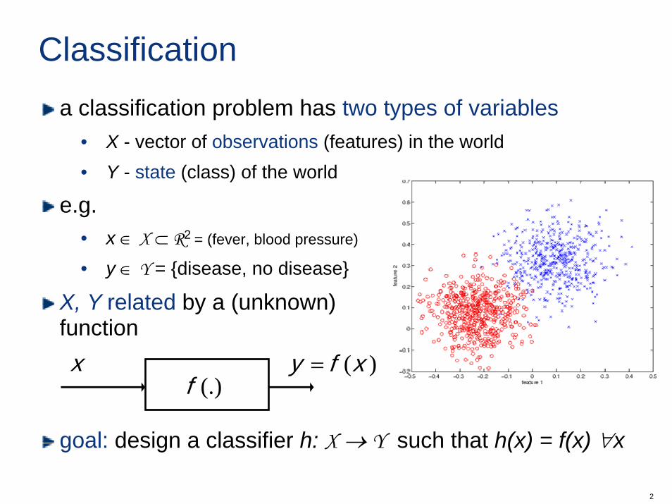
Classificationa classification problem has two types of variables

• X - vector of observations (features) in the world• Y - state (class) of the world

e.g. • x ∈ X ⊂ R2 = (fever, blood pressure)

• y ∈ Y = {disease, no disease}

X, Y related by a (unknown) function

goal: design a classifier h: X → Y such that h(x) = f(x) ∀x

)(xfy =x(.)f

3

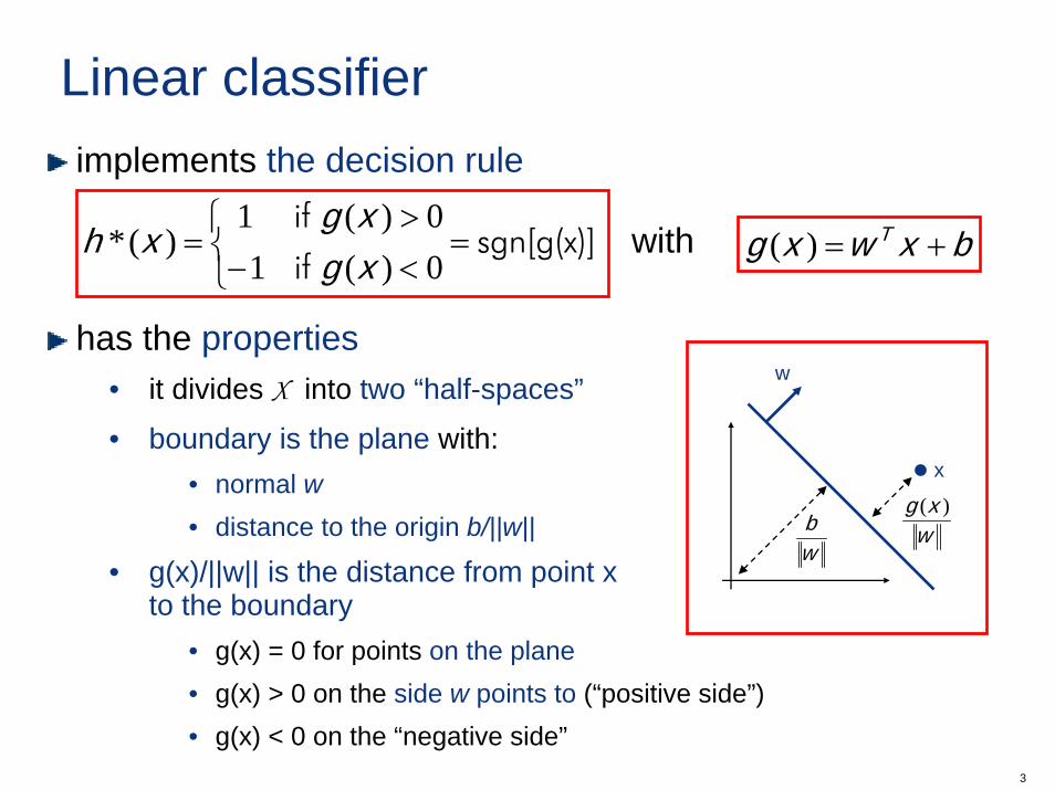
Linear classifier implements the decision rule

with

has the properties• it divides X into two “half-spaces”

• boundary is the plane with:• normal w• distance to the origin b/||w||

• g(x)/||w|| is the distance from point xto the boundary

• g(x) = 0 for points on the plane• g(x) > 0 on the side w points to (“positive side”)• g(x) < 0 on the “negative side”

bxwxg T +=)(⎩⎨⎧

=<−>

= sgn[g(x)] if

if

0)(10)(1

)(*xgxg

xh

w

wb

x

wxg )(

4

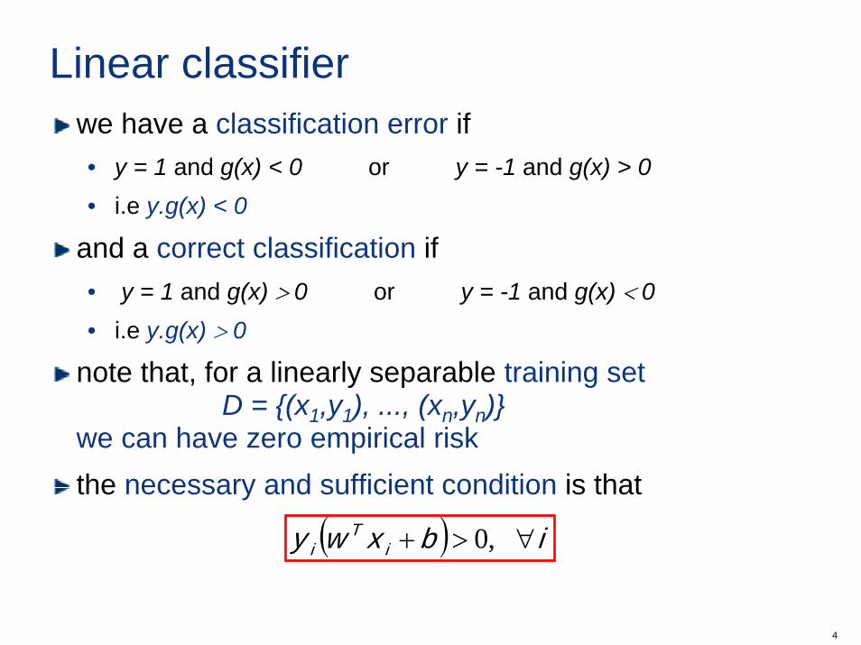
Linear classifierwe have a classification error if• y = 1 and g(x) < 0 or y = -1 and g(x) > 0• i.e y.g(x) < 0

and a correct classification if• y = 1 and g(x) > 0 or y = -1 and g(x) < 0• i.e y.g(x) > 0

note that, for a linearly separable training set D = {(x1,y1), ..., (xn,yn)}

we can have zero empirical riskthe necessary and sufficient condition is that

( ) ibxwy iT

i ∀>+ ,0

5

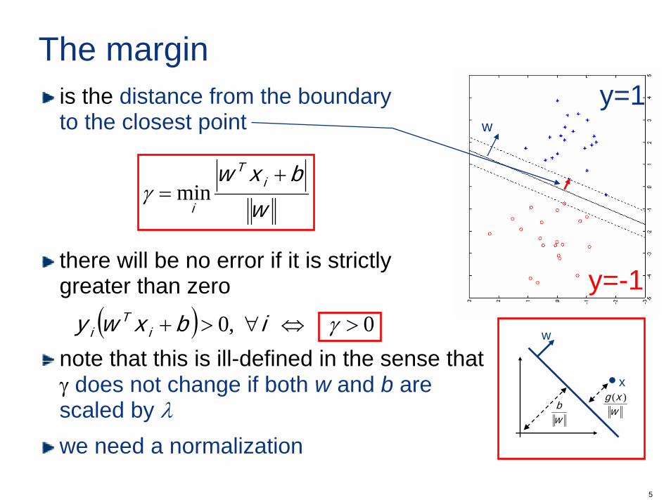
The marginis the distance from the boundaryto the closest point

there will be no error if it is strictlygreater than zero

note that this is ill-defined in the sense that γ does not change if both w and b are scaled by λwe need a normalization

( ) 0,0 >⇔∀>+ γ ibxwy iT

i

w

y=1

y=-1

w

wb

x

wxg )(

wbxw i

T

i

+= minγ

6

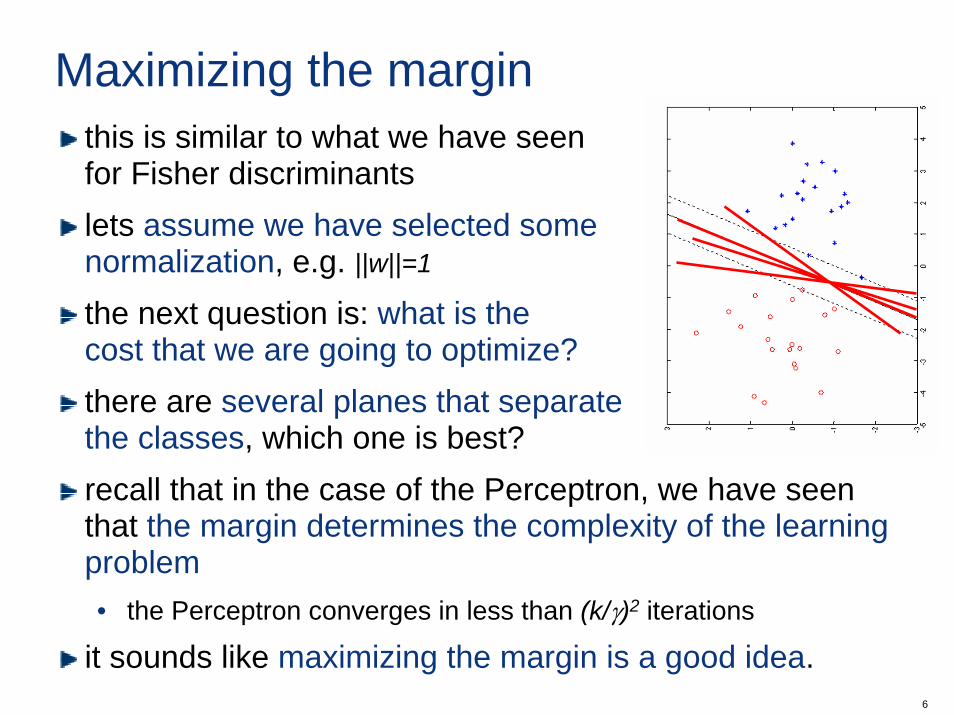
Maximizing the marginthis is similar to what we have seenfor Fisher discriminantslets assume we have selected somenormalization, e.g. ||w||=1

the next question is: what is thecost that we are going to optimize?there are several planes that separatethe classes, which one is best?recall that in the case of the Perceptron, we have seen that the margin determines the complexity of the learning problem• the Perceptron converges in less than (k/γ)2 iterations

it sounds like maximizing the margin is a good idea.

7

γ

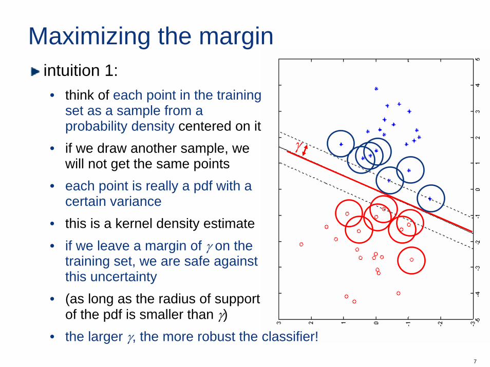
Maximizing the marginintuition 1:• think of each point in the training

set as a sample from a probability density centered on it

• if we draw another sample, we will not get the same points

• each point is really a pdf with a certain variance

• this is a kernel density estimate• if we leave a margin of γ on the

training set, we are safe against this uncertainty

• (as long as the radius of support of the pdf is smaller than γ)

• the larger γ, the more robust the classifier!

8

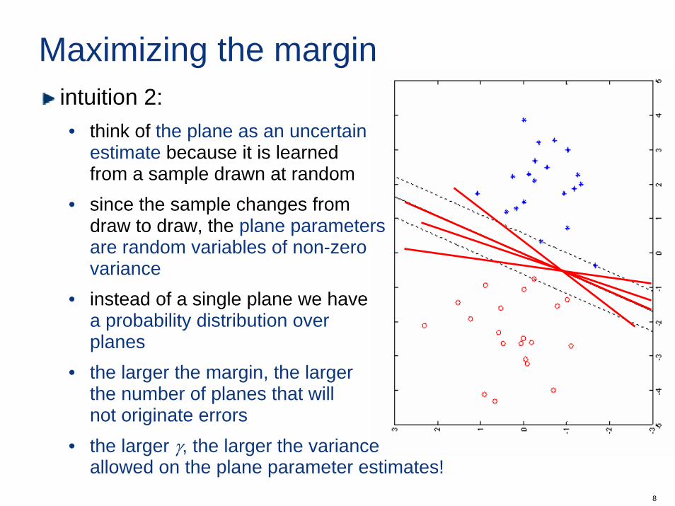
Maximizing the marginintuition 2:• think of the plane as an uncertain

estimate because it is learnedfrom a sample drawn at random

• since the sample changes fromdraw to draw, the plane parametersare random variables of non-zerovariance

• instead of a single plane we havea probability distribution overplanes

• the larger the margin, the largerthe number of planes that willnot originate errors

• the larger γ, the larger the variance allowed on the plane parameter estimates!

9

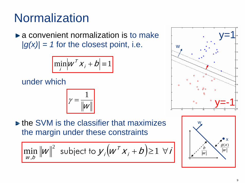
Normalizationa convenient normalization is to make |g(x)| = 1 for the closest point, i.e.

under which

the SVM is the classifier that maximizes the margin under these constraints

w

y=1

y=-1

w

wb

x

wxg )(

1min ≡+ bxw iT

i

w1

=γ

( ) ibxwyw iT

ibw∀≥+ tosubject 1min 2

,

10

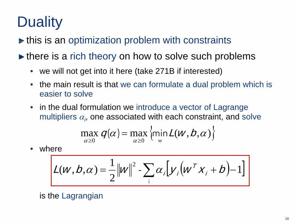
Dualitythis is an optimization problem with constraintsthere is a rich theory on how to solve such problems• we will not get into it here (take 271B if interested)• the main result is that we can formulate a dual problem which is

easier to solve• in the dual formulation we introduce a vector of Lagrange

multipliers αi, one associated with each constraint, and solve

• where

is the Lagrangian

{ }),,(maxmax00

αααα

bwLqw

min )( ≥≥

=

( )[ ] -i

∑ −+= 121),,( 2 bxwywbwL i

Tiiαα

11

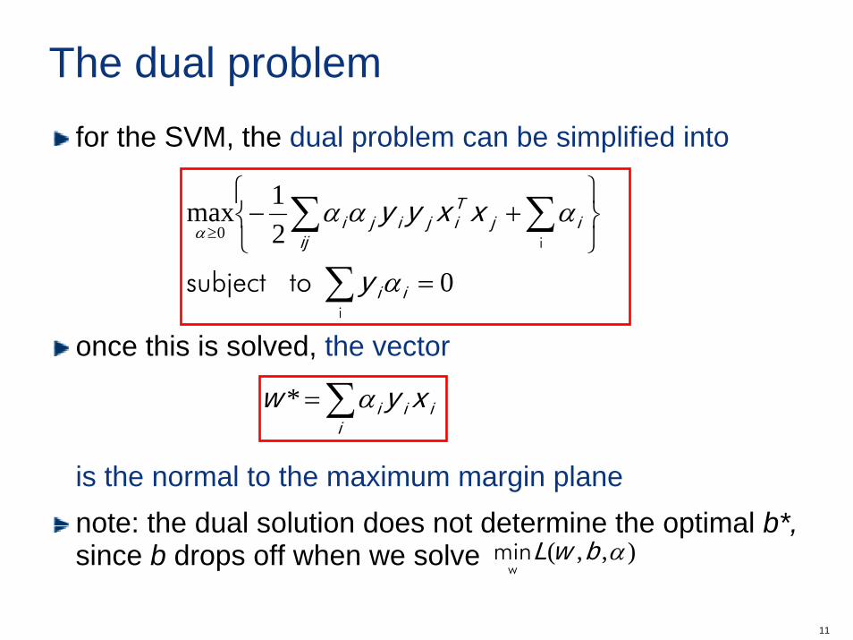
The dual problemfor the SVM, the dual problem can be simplified into

once this is solved, the vector

is the normal to the maximum margin planenote: the dual solution does not determine the optimal b*,since b drops off when we solve

0

21max

0

=⎭⎬⎫

⎩⎨⎧

+−

∑

∑∑≥

i

i

tosubject

ii

ijTij

ijiji

y

xxyy

α

αααα

∑=i

iii xyw α*

),,( αbwLw

min

12

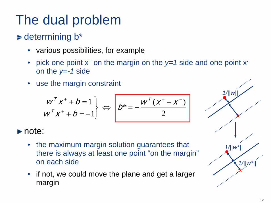
The dual problemdetermining b*• various possibilities, for example• pick one point x+ on the margin on the y=1 side and one point x-

on the y=-1 side• use the margin constraint

note:• the maximum margin solution guarantees that

there is always at least one point “on the margin”on each side

• if not, we could move the plane and get a largermargin

1/||w*||

1/||w*||

x

1/||w||

x2)(*

11 −+

+

+ +−=⇔

⎭⎬⎫

−=+=+ xxwb

bxwbxw T

T

T

13

Support vectors

αi=0

αi=0

αi>0

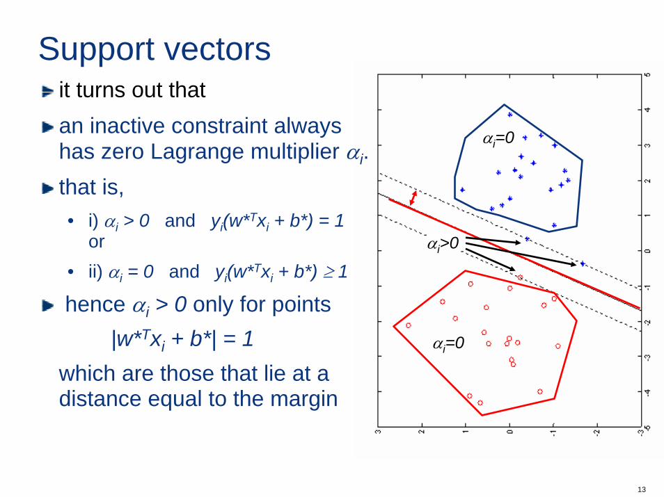
it turns out thatan inactive constraint always has zero Lagrange multiplier αi. that is, • i) αi > 0 and yi(w*Txi + b*) = 1

or• ii) αi = 0 and yi(w*Txi + b*) ≥ 1

hence αi > 0 only for points|w*Txi + b*| = 1

which are those that lie at a distance equal to the margin

14

Support vectors

αi=0

αi=0

αi>0

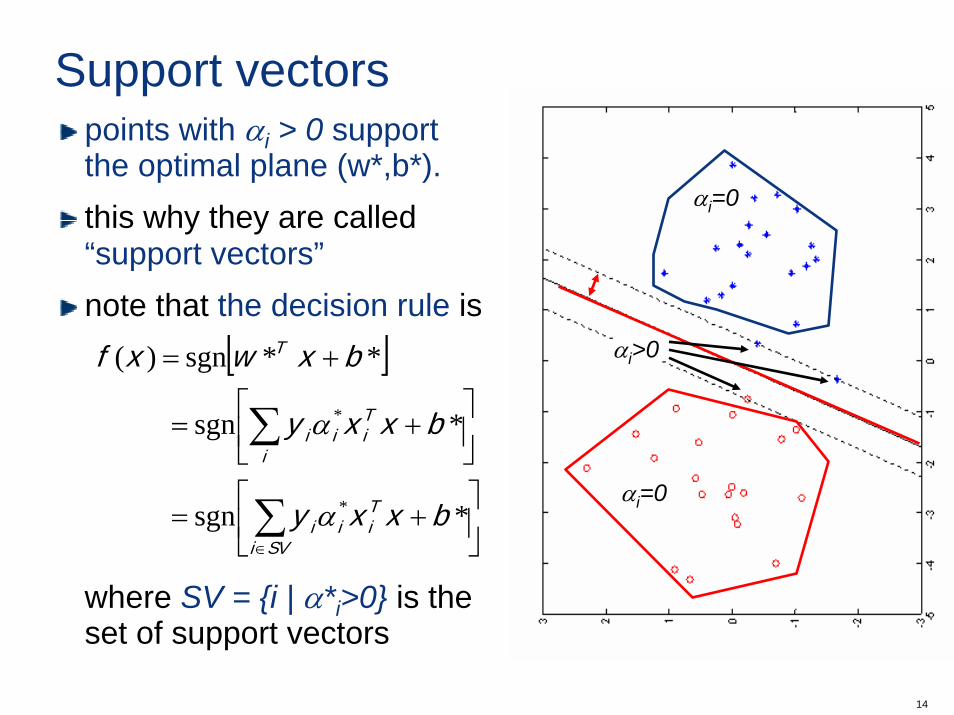
points with αi > 0 supportthe optimal plane (w*,b*).this why they are called“support vectors”note that the decision rule is

where SV = {i | α*i>0} is the set of support vectors

[ ]

⎥⎦

⎤⎢⎣

⎡+=

⎥⎦

⎤⎢⎣

⎡+=

+=

∑

∑

∈

*sgn

*sgn

**sgn)(

*

*

bxxy

bxxy

bxwxf

SVi

Tiii

i

Tiii

T

α

α

15

Support vectors

αi=0

αi=0

αi>0

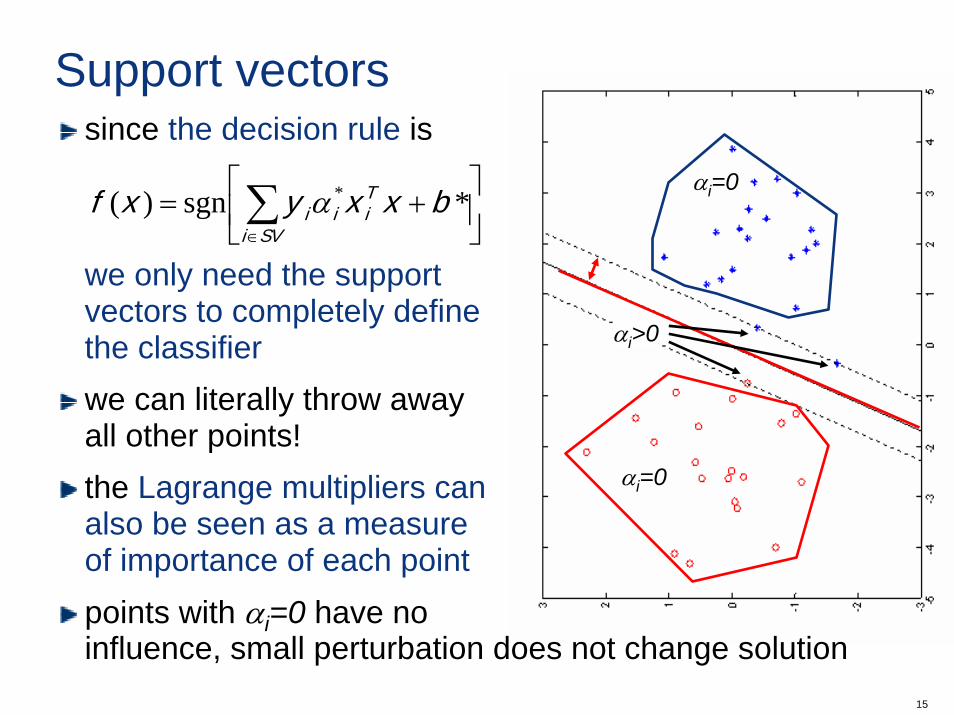
since the decision rule is

we only need the supportvectors to completely definethe classifierwe can literally throw awayall other points!the Lagrange multipliers canalso be seen as a measureof importance of each pointpoints with αi=0 have no influence, small perturbation does not change solution

⎥⎦

⎤⎢⎣

⎡+= ∑

∈

*sgn)( * bxxyxfSVi

Tiii α

16

The robustness of SVMswe talked a lot about the “curse of dimensionality”• number of examples required to achieve certain precision is

exponential in the number of dimensions

it turns out that SVMs are remarkably robust to dimensionality• not uncommon to see successful applications on 1,000D+ spaces

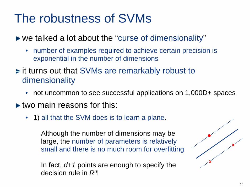
two main reasons for this:• 1) all that the SVM does is to learn a plane.

Although the number of dimensions may belarge, the number of parameters is relativelysmall and there is no much room for overfitting

In fact, d+1 points are enough to specify thedecision rule in Rd!

x

x

17

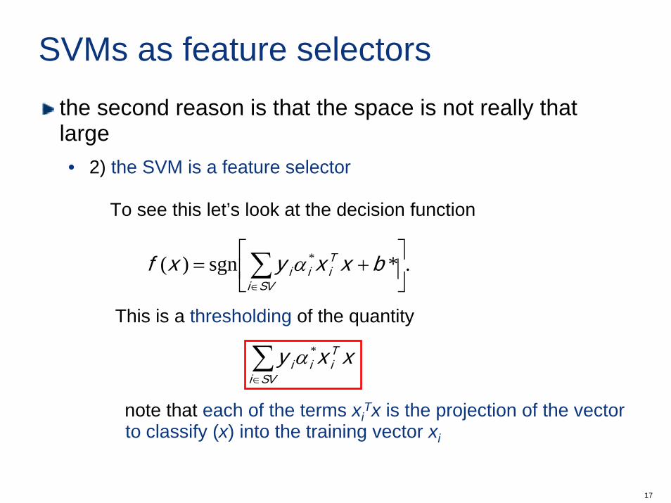
SVMs as feature selectorsthe second reason is that the space is not really that large• 2) the SVM is a feature selector

To see this let’s look at the decision function

This is a thresholding of the quantity

note that each of the terms xiTx is the projection of the vector

to classify (x) into the training vector xi

.*sgn)( *⎥⎦

⎤⎢⎣

⎡+= ∑

∈

bxxyxfSVi

Tiiiα

∑∈SVi

Tiii xxy *α

18

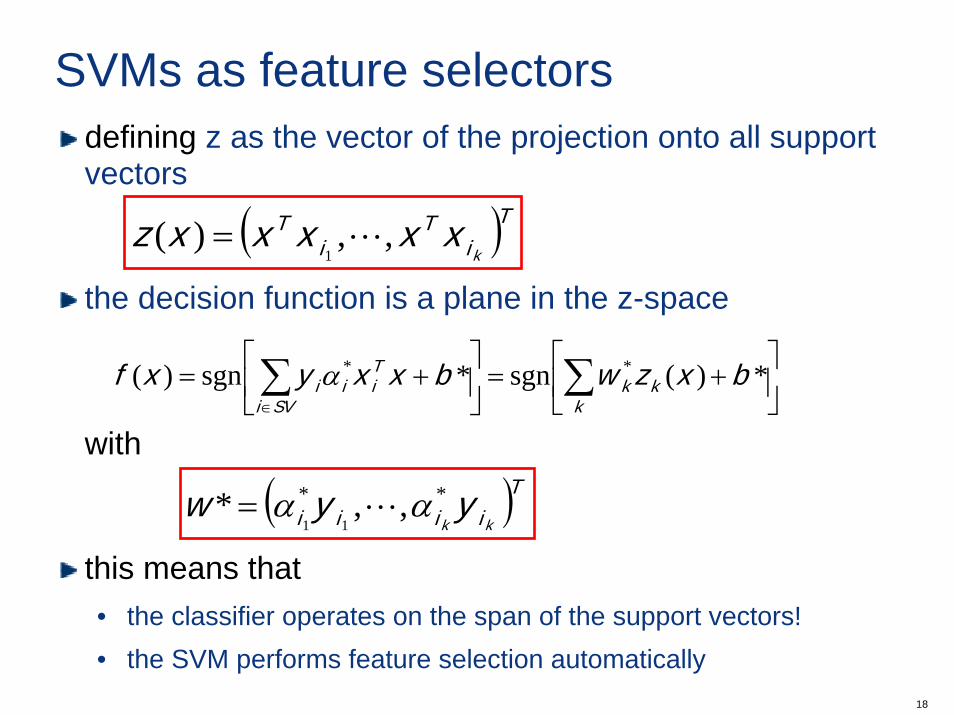
SVMs as feature selectorsdefining z as the vector of the projection onto all support vectors

the decision function is a plane in the z-space

with

this means that• the classifier operates on the span of the support vectors!• the SVM performs feature selection automatically

( )TiT

iT

kxxxxxz ,,)(

1L=

⎥⎦

⎤⎢⎣

⎡+=⎥

⎦

⎤⎢⎣

⎡+= ∑∑

∈

*)(sgn*sgn)( ** bxzwbxxyxf kk

kSVi

Tiii α

( )Tiiii kkyyw ** ,,*

11αα L=

19

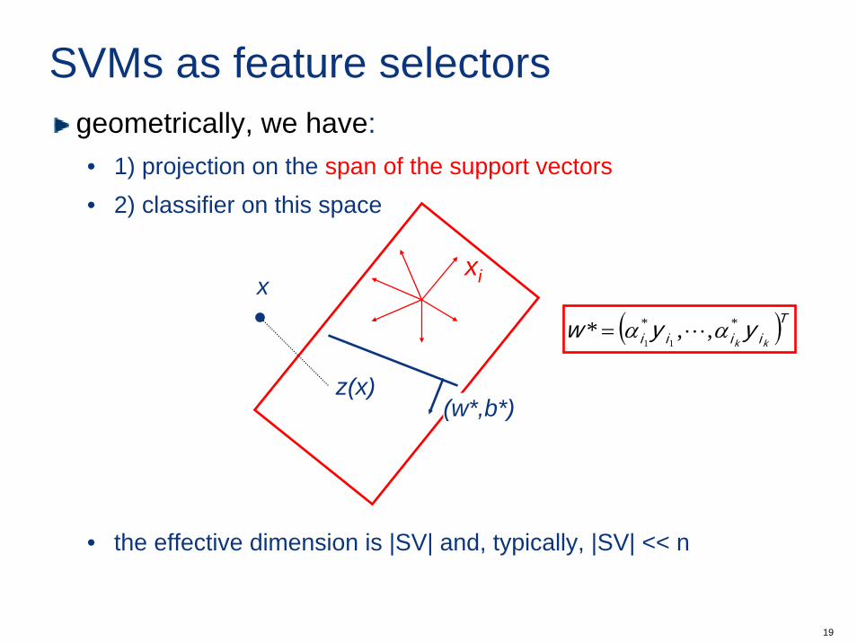
SVMs as feature selectorsgeometrically, we have:• 1) projection on the span of the support vectors• 2) classifier on this space

• the effective dimension is |SV| and, typically, |SV| << n

( )Tiiii kkyyw ** ,,*

11αα L=

xix

z(x)(w*,b*)

20

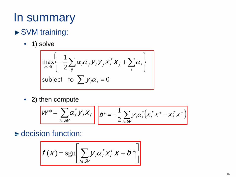
In summarySVM training:• 1) solve

• 2) then compute

decision function:

0

21max

0

=⎭⎬⎫

⎩⎨⎧

+−

∑

∑∑≥

i

i

tosubject

ii

ijTij

ijiji

y

xxyy

α

αααα

∑∈

=SVi

iii xyw ** α ( )−+

∈

+−= ∑ xxxxyb Ti

Tii

SVii

*

21* α

⎥⎦

⎤⎢⎣

⎡+= ∑

∈

*sgn)( * bxxyxfSVi

Tiii α

21

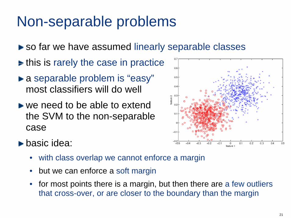
Non-separable problemsso far we have assumed linearly separable classesthis is rarely the case in practicea separable problem is “easy”most classifiers will do wellwe need to be able to extendthe SVM to the non-separablecasebasic idea:• with class overlap we cannot enforce a margin• but we can enforce a soft margin• for most points there is a margin, but then there are a few outliers

that cross-over, or are closer to the boundary than the margin

22

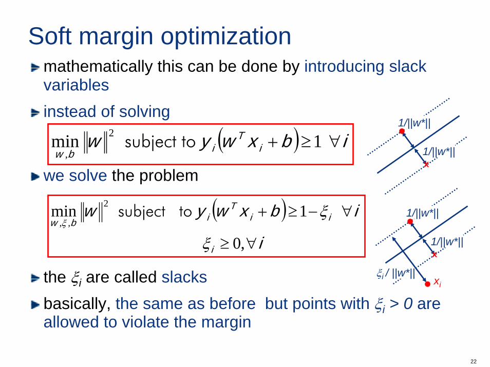
Soft margin optimizationmathematically this can be done by introducing slack variablesinstead of solving

we solve the problem

the ξi are called slacksbasically, the same as before but points with ξi > 0 are allowed to violate the margin

( ) ibxwyw iT

ibw∀≥+ tosubject 1min 2

,

( )i

ibxwyw

i

iiT

ibw

∀≥

∀−≥+

,0

1min 2

,,

ξ

ξξ

tosubject

1/||w*||

1/||w*||

x

ξi / ||w*||xi

1/||w*||

1/||w*||

x

23

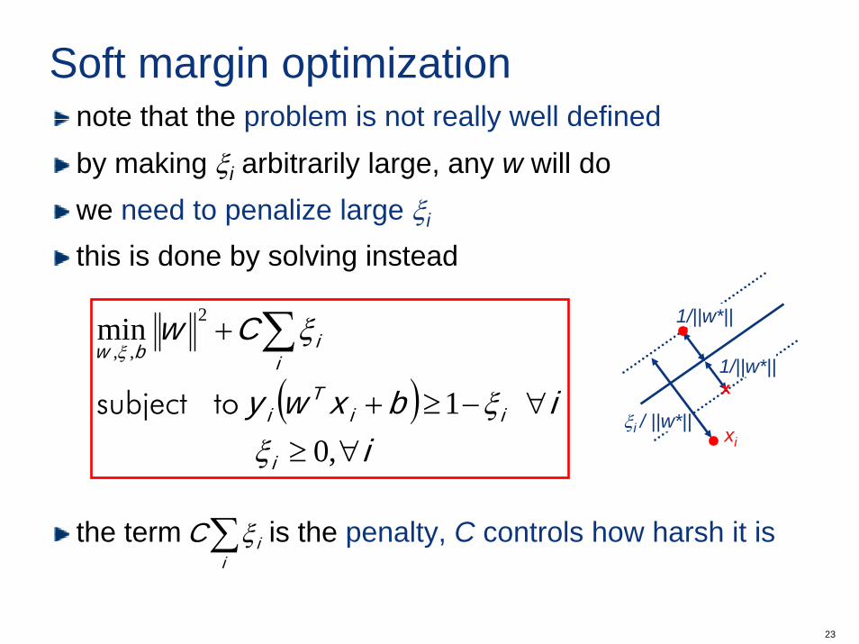
Soft margin optimizationnote that the problem is not really well definedby making ξi arbitrarily large, any w will dowe need to penalize large ξi

this is done by solving instead

the term is the penalty, C controls how harsh it is

( )i

ibxwy

Cw

i

iiT

i

iibw

∀≥∀−≥+

+ ∑

,01

min 2

,,

ξξ

ξξ

tosubject

1/||w*||

1/||w*||

x

ξi / ||w*||xi

∑i

iC ξ

24

The dual problem

αi=0

αi=0

0 < αi < c

*

*

αi = c

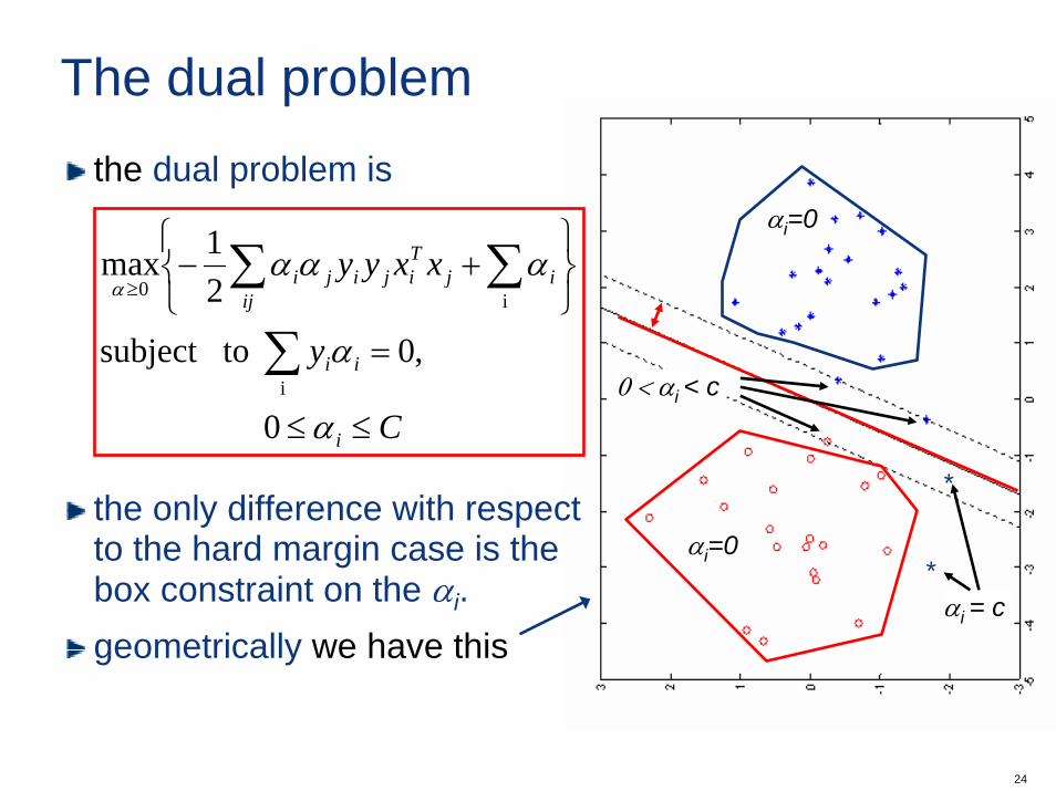
the dual problem is

the only difference with respect to the hard margin case is the box constraint on the αi.geometrically we have this

C

y

xxyy

i

ii

ijTij

ijiji

≤≤

=⎭⎬⎫

⎩⎨⎧

+−

∑

∑∑≥

α

α

αααα

0

,0 tosubject

21max

i

i0

25

Support vectors

αi=0

αi=0

0 < αi < c

*

*

αi = c

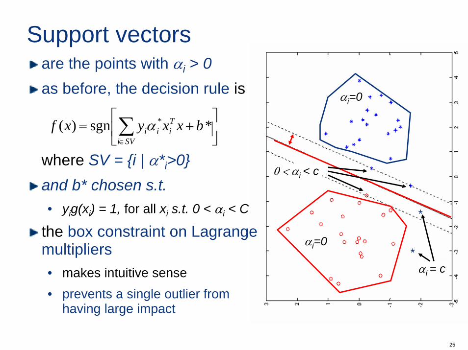
are the points with αi > 0as before, the decision rule is

where SV = {i | α*i>0}and b* chosen s.t.• yig(xi) = 1, for all xi s.t. 0 < αi < C

the box constraint on Lagrangemultipliers• makes intuitive sense• prevents a single outlier from

having large impact

⎥⎦

⎤⎢⎣

⎡+= ∑

∈

*sgn )( * bxxyxfSVi

Tiiiα

26

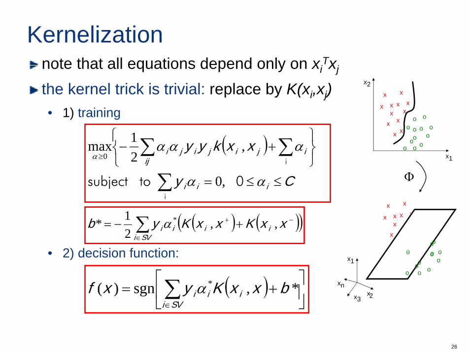
Kernelizationnote that all equations depend only on xi

Txj

the kernel trick is trivial: replace by K(xi,xj)• 1) training

• 2) decision function:

xx

x

x

x

xxx

xx

xx

oo

o

o

ooo

o

oooo

x1

x2

xx

x

x

x

xxx

xx

xx

oo

o

o

ooo

o

oooo

x1

x3x2

xn

Φ

( )

Cy

xxkyy

iii

ijijij

iji

≤≤=⎭⎬⎫

⎩⎨⎧

+−

∑

∑∑≥

αα

αααα

0 tosubject

i

i

,0

,21max

0

( ) ( )( )−+

∈

+−= ∑ xxKxxKyb iiiSVi

i ,,21* *α

( ) ⎥⎦

⎤⎢⎣

⎡+= ∑

∈

*,sgn)( * bxxKyxfSVi

iii α

27

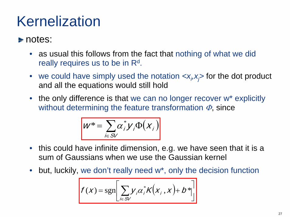
Kernelizationnotes:• as usual this follows from the fact that nothing of what we did

really requires us to be in Rd.• we could have simply used the notation <xi,xj> for the dot product

and all the equations would still hold• the only difference is that we can no longer recover w* explicitly

without determining the feature transformation Φ, since

• this could have infinite dimension, e.g. we have seen that it is a sum of Gaussians when we use the Gaussian kernel

• but, luckily, we don’t really need w*, only the decision function

( )∑∈

Φ=SVi

iii xyw ** α

( ) ⎥⎦

⎤⎢⎣

⎡+= ∑

∈

*,sgn)( * bxxKyxfSVi

iii α

28

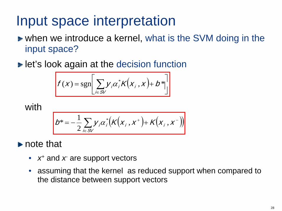
Input space interpretationwhen we introduce a kernel, what is the SVM doing in the input space?let’s look again at the decision function

with

note that • x+ and x- are support vectors• assuming that the kernel as reduced support when compared to

the distance between support vectors

( ) ⎥⎦

⎤⎢⎣

⎡+= ∑

∈

*,sgn)( * bxxKyxfSVi

iii α

( ) ( )( )−+

∈

+−= ∑ xxKxxKyb iiiSVi

i ,,21* *α

29

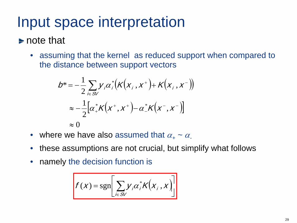
Input space interpretationnote that • assuming that the kernel as reduced support when compared to

the distance between support vectors

• where we have also assumed that α+ ~ α-

• these assumptions are not crucial, but simplify what follows• namely the decision function is

( )⎥⎦

⎤⎢⎣

⎡= ∑

∈SViiii xxKyxf ,sgn)( *α

( ) ( )( )

( ) ( )[ ]

0

,,21

,,21*

**

*

≈

−−≈

+−=

−−−

+++

−+

∈∑

xxKxxK

xxKxxKyb iiiSVi

i

αα

α

30

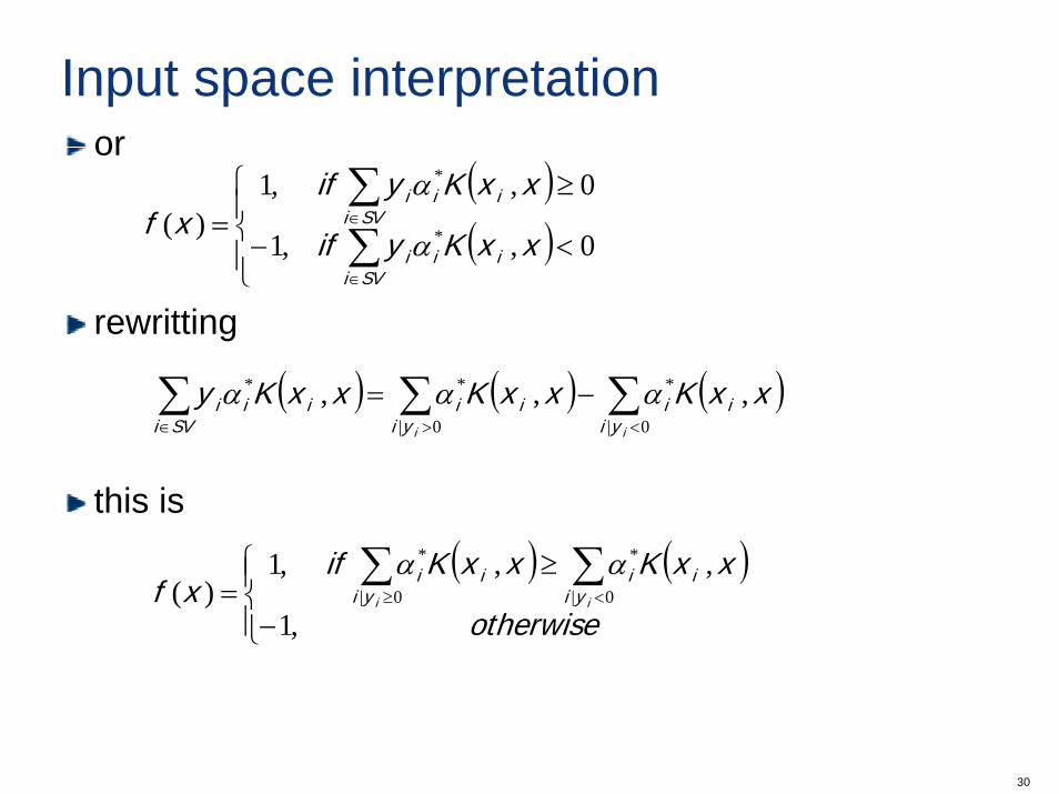
Input space interpretationor

rewritting

this is

( )( )⎪⎩

⎪⎨⎧

<−

≥=

∑∑

∈

∈

0,,1

0,,1)( *

*

SViiii

SViiii

xxKyif

xxKyifxf

α

α

( ) ( ) ( )∑∑∑<>∈

−=0|

*

0|

** ,,,ii yi

iiyi

iiSVi

iii xxKxxKxxKy ααα

( ) ( )⎪⎩

⎪⎨⎧

−

≥=

∑∑<≥

otherwise

xxKxxKifxf ii yi

iiyi

ii

,1

,,,1)( 0|

*

0|

* αα

31

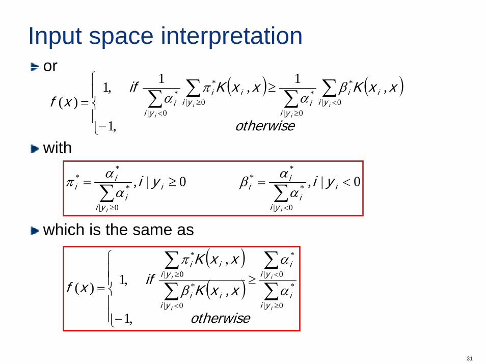
Input space interpretationor

with

which is the same as

( ) ( )⎪⎩

⎪⎨

⎧

−

≥=

∑∑∑∑ <≥

≥<

otherwise

xxKxxKifxf i

i

i

i

yiii

yiiyi

ii

yii

,1

,1,1,1)( 0|

*

0|

*0|

*

0|

* βα

πα

0|,0|,

0|

*

**

0|

*

** <=≥=

∑∑<≥

i

yii

iii

yii

ii yiyi

ii

ααβ

ααπ

( )( )

⎪⎪⎩

⎪⎪⎨

⎧

−

≥= ∑∑

∑∑

≥

<

<

≥

otherwise

xxK

xxKifxf

i

i

i

i

yii

yii

yiii

yiii

,1

,

,,1)(

0|

*0|

*

0|

*0|

*

α

α

β

π

32

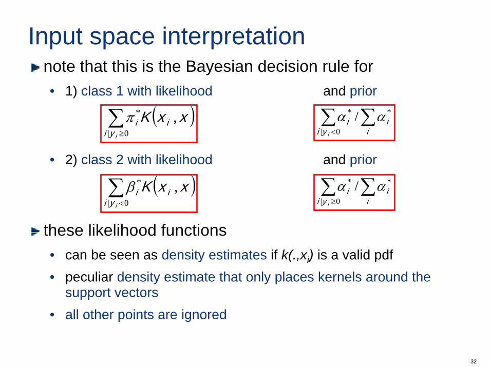
Input space interpretationnote that this is the Bayesian decision rule for• 1) class 1 with likelihood and prior

• 2) class 2 with likelihood and prior

these likelihood functions • can be seen as density estimates if k(.,xi) is a valid pdf• peculiar density estimate that only places kernels around the

support vectors• all other points are ignored

( )∑≥0|

* ,iyi

ii xxKπ ∑∑< i

iyi

ii

*

0|

* / αα

( )∑<0|

* ,iyi

ii xxKβ ∑∑≥ i

iyi

ii

*

0|

* / αα

33

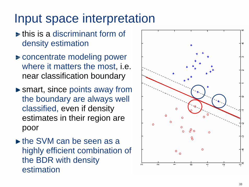
Input space interpretationthis is a discriminant form of density estimationconcentrate modeling power where it matters the most, i.e. near classification boundarysmart, since points away from the boundary are always well classified, even if density estimates in their region are poorthe SVM can be seen as a highly efficient combination of the BDR with density estimation

34

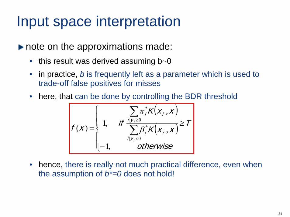
Input space interpretationnote on the approximations made:• this result was derived assuming b~0• in practice, b is frequently left as a parameter which is used to

trade-off false positives for misses• here, that can be done by controlling the BDR threshold

• hence, there is really not much practical difference, even when the assumption of b*=0 does not hold!

( )( )

⎪⎪⎩

⎪⎪⎨

⎧

−

≥= ∑∑

<

≥

otherwise

TxxK

xxKifxf

i

i

yiii

yiii

,1

,

,,1)(

0|

*0|

*

β

π

35

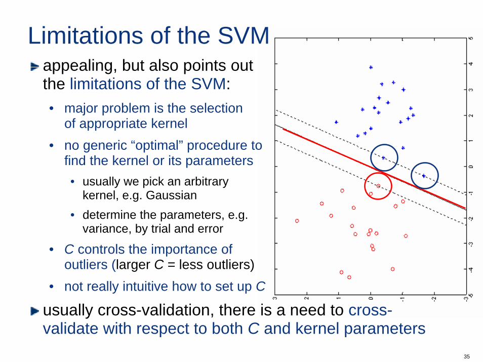
Limitations of the SVMappealing, but also points outthe limitations of the SVM:• major problem is the selection

of appropriate kernel• no generic “optimal” procedure to

find the kernel or its parameters• usually we pick an arbitrary

kernel, e.g. Gaussian• determine the parameters, e.g.

variance, by trial and error

• C controls the importance of outliers (larger C = less outliers)

• not really intuitive how to set up C

usually cross-validation, there is a need to cross-validate with respect to both C and kernel parameters

36

Practical implementationsin practice we need an algorithm for solving the optimization problem of the training stage• this is still a complex problem• there has been a large amount of research in this area• coming up with “your own” algorithm is not going to be

competitive• luckily there are various packages available, e.g.:

• libSVM: http://www.csie.ntu.edu.tw/~cjlin/libsvm/• SVM light: http://www.cs.cornell.edu/People/tj/svm_light/• SVM fu: http://five-percent-nation.mit.edu/SvmFu/• various others (see http://www.support-vector.net/software.html)

• also many papers and books on algorithms (see e.g. B. Schölkopfand A. Smola. Learning with Kernels. MIT Press, 2002)

37