Embed Size (px)
Citation preview
1
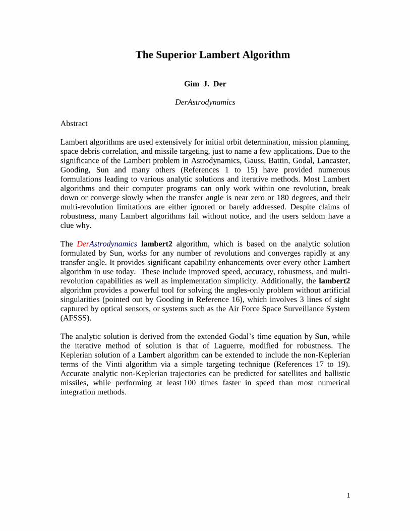
The Superior Lambert Algorithm
Gim J. Der
DerAstrodynamics
Abstract
Lambert algorithms are used extensively for initial orbit determination, mission planning,
space debris correlation, and missile targeting, just to name a few applications. Due to the
significance of the Lambert problem in Astrodynamics, Gauss, Battin, Godal, Lancaster,
Gooding, Sun and many others (References 1 to 15) have provided numerous
formulations leading to various analytic solutions and iterative methods. Most Lambert
algorithms and their computer programs can only work within one revolution, break
down or converge slowly when the transfer angle is near zero or 180 degrees, and their
multi-revolution limitations are either ignored or barely addressed. Despite claims of
robustness, many Lambert algorithms fail without notice, and the users seldom have a
clue why.
The DerAstrodynamics lambert2 algorithm, which is based on the analytic solution
formulated by Sun, works for any number of revolutions and converges rapidly at any
transfer angle. It provides significant capability enhancements over every other Lambert
algorithm in use today. These include improved speed, accuracy, robustness, and multi-
revolution capabilities as well as implementation simplicity. Additionally, the lambert2
algorithm provides a powerful tool for solving the angles-only problem without artificial
singularities (pointed out by Gooding in Reference 16), which involves 3 lines of sight
captured by optical sensors, or systems such as the Air Force Space Surveillance System
(AFSSS).
The analytic solution is derived from the extended Godal’s time equation by Sun, while
the iterative method of solution is that of Laguerre, modified for robustness. The
Keplerian solution of a Lambert algorithm can be extended to include the non-Keplerian
terms of the Vinti algorithm via a simple targeting technique (References 17 to 19).
Accurate analytic non-Keplerian trajectories can be predicted for satellites and ballistic
missiles, while performing at least 100 times faster in speed than most numerical
integration methods.
2
Introduction
In 1991, Klumpp of JPL (Reference 10) compared the performance of numerous Lambert
algorithms over the last two hundred years and declared the Gooding Lambert algorithm
the winner. The Gooding Lambert algorithm (Reference 7), which originates from the
Lancaster-Blanchard analytic solution (Reference 6), computes an initial guess of the
universal iteration parameter for a high order Halley iterative method. Since Klumpp’s
limited (115 samples) results of the Gooding Lambert algorithm showed speed, accuracy,
robustness, and applicability for multiple revolutions, one might be inclined to ask how
DerAstrodynamics lambert2 algorithm can be better. Simply put, it operates on the same
theory, but with no starting and convergence problems, proven multi-revolution
capability and includes easily more accurate non-Keplerian solutions of Vinti. The
outstanding works of the late Professor Sun, regarding the multi-revolution Lambert
problem, have been invaluable in developing this analytic solution.
Similar to the analytic solution of a Kepler algorithm, the analytic solution of a Lambert
algorithm is not in closed form; an iterative method must be used to deduce a numerical
solution. Contrary to the analytic solution of a Kepler algorithm, the analytic solution of a
Lambert algorithm should be understood and visualized using any formulation, with or
without universal variables. Any multiple-revolution Lambert problem has only elliptic
solutions, and the conic solutions for trajectories less than one revolution can be simple,
if the independent or unknown iteration parameter is chosen wisely. Since the initial
value for the unknown iteration parameter of the lambert2 algorithm can be visualized
and bounded within known limits, there is no need for intelligent starters, averaging, or
binary search methods. High-order iterative methods are needed for robustness, but it can
be proved that failures still exist as in the examples of the DerAstrodynamics kepler1
algorithm. In Klumpp’s report, Conway indicated that all other high-order methods fail.
Conway also claimed, without proof, the Laguerre iterative method has never been
known to fail. In a space debris study, Der encountered many cases that the Conway-
Laguerre iterative method can fail at the rate of one in a thousand. Der modified the
implementation of the Laguerre iterative method to ensure Conway’s infallibility claim,
yet still achieve rapid convergence.
The lambert2 algorithm is the fastest, most accurate, robust and multi-revolution
Lambert algorithm today. If a Lambert algorithm uses the Newton method for the
iterative procedure, then it cannot be robust. The principal advantage of the lambert2
algorithm is that the unknown iteration parameters for any revolution can be visually
estimated to within a very small range before the iterations begin. This presents a user
with the feel and some physical meaning of the converged numerical solutions. In the
unlikely event of failure, the user can easily find out the cause. The lambert2 algorithm
is also compact and contains only two functions. The lines-of-code for the main function
is approximately 200, and that of the minimum time subroutine is about 50. It can solve
for elliptic orbits of any revolution, and parabolic and hyperbolic orbits of less than one
revolution.
3
1
2
Orbit 1
Orbit 2
Earth(Central body)
1t
t
2r
2v
1r
1v
t1v
t2v
Kepleriantransfer
trajectory
2
The Lambert Problem
Given: r , r , t , t
Find: v (t ) = , v (t ) =
2
1
1 21
2t1v
t2v
= 1 t1v
1v
= 2 t2
v2
v
Then compute:
v
v
v
v
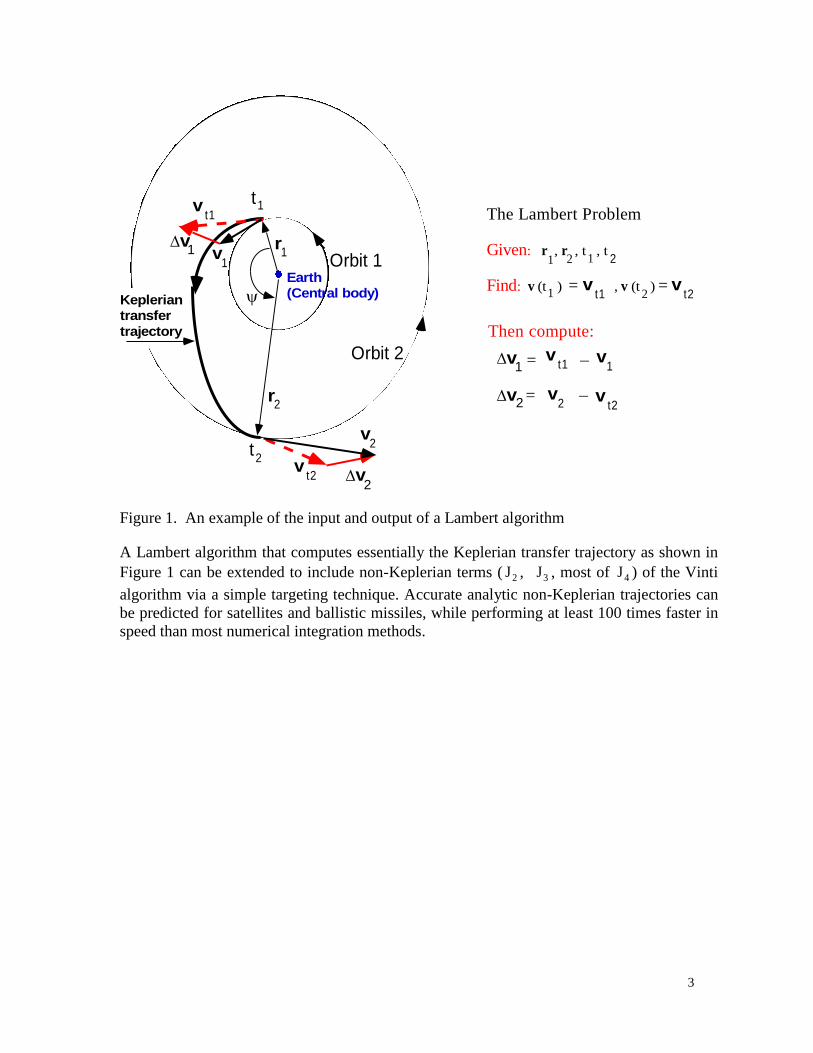
Figure 1. An example of the input and output of a Lambert algorithm
A Lambert algorithm that computes essentially the Keplerian transfer trajectory as shown in
Figure 1 can be extended to include non-Keplerian terms ( 2J , 3J , most of 4J ) of the Vinti
algorithm via a simple targeting technique. Accurate analytic non-Keplerian trajectories can
be predicted for satellites and ballistic missiles, while performing at least 100 times faster in
speed than most numerical integration methods.
4
General Formulation of the Lambert Problem
The method of solving the problems of Kepler and Lambert are practically the same. The
Kepler problem is an initial value problem of solving the equations of motion
2
2 3
d=
d t r
rr (1)
to find the position and velocity vectors )( 2tr and )( 2tv at any given time 2t ; given the
initial position and velocity vectors 11 = t )( rr and 11 = t )( vv at a given initial time 1t , and
is the gravitational constant for the central body. The classical theory ends with solving for
the solution of one unknown, the eccentric anomaly E, in the Kepler Equation:
F (E) = E e sin E 0 (2)
where the mean anomaly M and the eccentricity e can be computed from the given times 1t ,
2t and the initial state vector of 1r and 1v .
The Lambert problem is a two-point boundary value problem of solving the same equations
of motion (1) to find the velocity vectors )( 1tv at a given initial time 1t and )( 2tv at a given
time 2t ; given the position vectors 1r and 2r at the respective times 1t and 2t (Figure 1).
The classical theory (Gauss or Battin) solves two equations for two unknowns, but can be
deduced to solve for one unknown, the semi-major axis, a, in the Lambert Equation:
3aF (a ) = [ ( sin ) sin ) ] t 0
(3)
where t = 2t and 1t = 0 without loss of generality, and and are functions of the semi-
major axis.
Using Sun’s notations of Reference 5, the Lambert Equation for multi-revolution elliptic
orbits can be expressed as:
F ( x ) = ( x ) y) N 0 (4)
where x is the only unknown or independent variable to be solved for, y is a function of x,
is the normalized time computed from the given 1t , 2t , 1r , 2r , , and N 0 is the orbit
revolution number. When N = 0, equation (4) can be reduced to equation (3) with different
notations, while x is essentially a function of the semi-major axis. This beautiful equation (4)
provides the foundation to develop an algorithm and computational procedure for any
revolution of elliptic orbits without difficulty. When N is greater than zero, parabolic and
hyperbolic transfer orbits do not exist. The actual expressions of equation (4), including those
for parabolic and hyperbolic orbits, are included in Appendix A. The functions ( x ) and
y) are defined later by equation (13) in the Computational Procedure section.
5
The transcendental Kepler equation (2), and Lambert equations (3) and (4) do not allow any
opportunity for closed form solutions, even though there is only one unknown. Numerous
iterative methods that are specific to each formulation and independent variable exist, and the
use of hyper-geometric functions is one of Battin’s tricks. However, simple iterative methods
such as those of Newton, Halley and Laguerre are available, if the first and/or the second
derivatives of the functions, F (E) , F (a ) , F ( x ) , can be derived.
The Laguerre method as stated in Reference 13 is intended to solve the roots of a polynomial
equation of degree n. If the first and second derivatives of F ( x ) are respectively F ( x ) and
F ( x ) , then the Lambert equation (4) can be solved by the iterative formula
ii+1 i
22ii i i i
i
n F (x )for i 1, 2, ..
F (x )F (x ) (n 1) F (x ) n (n 1) F (x )F (x )
F (x )
x x
(5)
where the degree n = 1, 2, . . . The sign ambiguity in equation (5) is resolved by taking the
sign of the numerical value of F ( x ) . If n = 1, then equation (5) is reduced to the iterative
method of Newton. With an open mind and the lightning speed of a modern computer,
robustness can be achieved by varying n. When Newton’s method is used, a reasonable initial
guess of 1x must be estimated, and some authors have developed sophisticated formulae just
for this purpose. Similarly, Gooding of Reference 7 also used complicated starting guesses
for the Halley method. Unlike the Newton and Halley methods, the Laguerre method requires
that the initial starting value, 1x for i = 1 in equation (5) can be “just a rough guess”, 0.5
for any elliptic orbit or revolution. Many Lambert algorithms use the Newton method and
robustness is compromised. These Lambert algorithms break down if the Newton method
fails and usually the initial guess is poor. If n is allowed to vary in the Laguerre method, then
the chance of getting a converged solution increases dramatically. The value of n, which is
arbitrary, is initially set to 2 in the lambert2 algorithm.
In addition, the physics of the Lambert problem and the specific formulation of a Lambert
algorithm dictate the limits of the independent variable. The Sun Formulation requires the
independent variable x be defined as x 1 for elliptic orbits for all N, and x 1 for
parabolic orbits, and x 1 for hyperbolic orbits when N = 0. When x is bounded within
limits, the estimate of the initial guess is simple. For example, if the given position vectors
requires that 1 x 0 , then the initial rough guess can be chosen as 1x 0.5 . The
Laguerre method, which is very forgiving, has not yet failed to converge to correct solutions.
If this “rough guess” for x is satisfactory, then the lambert2 algorithm can be used to solve
multi-revolution Lambert problems with N = 0, 1, 2, ….
The general formulation of the Lambert problem as presented above is simple. Other general
formulations of solving two equations and two unknowns, which are complicated, will not be
discussed. The Primer Vector approach (Reference 11) and Series Reversion/Inversion
method (Reference 12) are also not recommended and discussed later in the Conclusions. For
completeness, Sun’s expressions for F ( x ), F ( x ) and F ( x ) are given in Appendix A.
6
The Sun Theory for the Multi-Revolution Lambert Problem
This section may be skipped for the readers not interested in the details of the Sun theory.
In the following presentation, only elliptic orbits of multi-revolution will be described and
Sun’s notations of Reference 5 are used unless otherwise specified. Lancaster and Gooding
of References 6 and 7 presented almost the same theory with different notations and iterative
methods. When two position vectors, 1r and 2r are given at the respective times 1t and 2t ,
the central angle or transfer angle, , between 1r and 2r can be identified by a value of
less than, equal to or greater than 180 degrees. Let0
1 1 2
1 2
cos [ ]r r
r r
r1
r2
h = r x r21
k = (0, 0, 1)
direct transfer orbit
(inclination <= 90 )
r1
r2
h = r x r21
k = (0, 0, 1)
retrograde transfer orbit
(inclination > 90 )
r1
r2
h = r x r21
k = (0, 0, 1)
o o
o = 2
= k h = k h
o = <
o = 2
o = <
r1
r2
h = r x r21
Transfer
orbit
direction
defined
by input
in-plane
in-plane
out-of-plane
out-of-plane
7
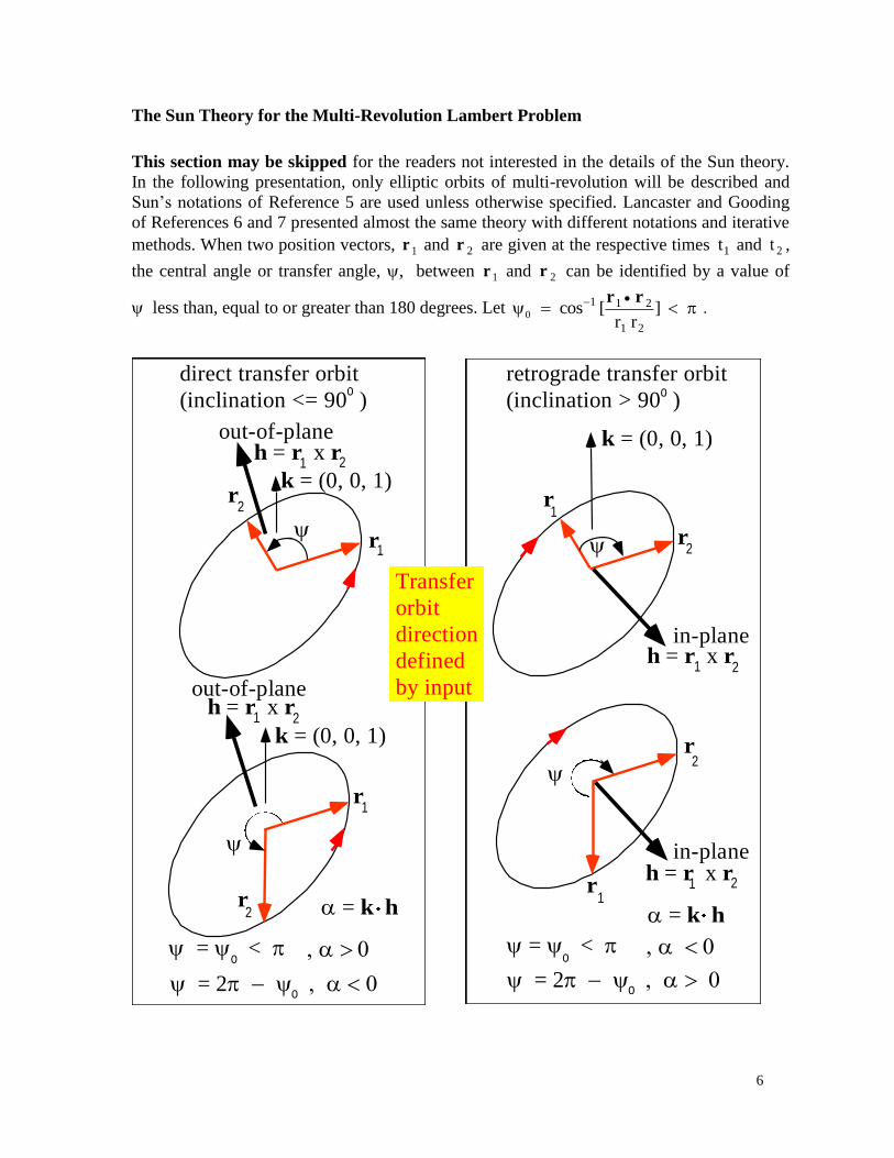
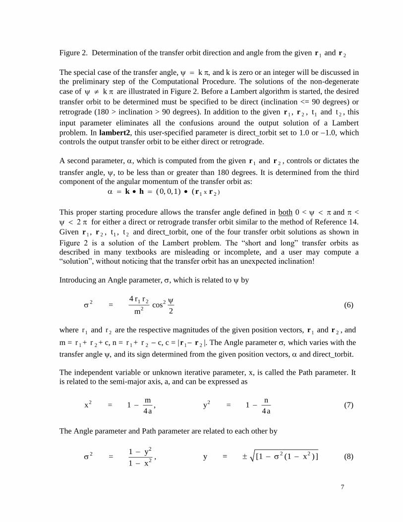
Figure 2. Determination of the transfer orbit direction and angle from the given 1r and 2r
The special case of the transfer angle, k and k is zero or an integer will be discussed in
the preliminary step of the Computational Procedure. The solutions of the non-degenerate
case of k are illustrated in Figure 2. Before a Lambert algorithm is started, the desired
transfer orbit to be determined must be specified to be direct (inclination <= 90 degrees) or
retrograde (180 > inclination > 90 degrees). In addition to the given 1r , 2r , 1t and 2t , this
input parameter eliminates all the confusions around the output solution of a Lambert
problem. In lambert2, this user-specified parameter is direct_torbit set to 1.0 or 1.0, which
controls the output transfer orbit to be either direct or retrograde.
A second parameter, , which is computed from the given 1r and 2r , controls or dictates the
transfer angle, , to be less than or greater than 180 degrees. It is determined from the third
component of the angular momentum of the transfer orbit as:
1 2x )(0, 0,1) ( k h r r
This proper starting procedure allows the transfer angle defined in both 0 < and <
for either a direct or retrograde transfer orbit similar to the method of Reference 14.
Given 1r , 2r , 1t , 2t and direct_torbit, one of the four transfer orbit solutions as shown in
Figure 2 is a solution of the Lambert problem. The “short and long” transfer orbits as
described in many textbooks are misleading or incomplete, and a user may compute a
“solution”, without noticing that the transfer orbit has an unexpected inclination!
Introducing an Angle parameter, , which is related to by
1 22 2
2
4 r r= cos
2m
(6)
where 1r and 2r are the respective magnitudes of the given position vectors, 1r and 2r , and
m = 1r + 2r + c, n = 1r + 2r c, c = | 1r 2r |. The Angle parameter which varies with the
transfer angle and its sign determined from the given position vectors, and direct_torbit.
The independent variable or unknown iterative parameter, x, is called the Path parameter. It
is related to the semi-major axis, a, and can be expressed as
2 mx = 1
4a , 2 n
y = 14a
(7)
The Angle parameter and Path parameter are related to each other by
2
2
2
1 y=
1 x
,
2 2y = [1 (1 x )] (8)
8
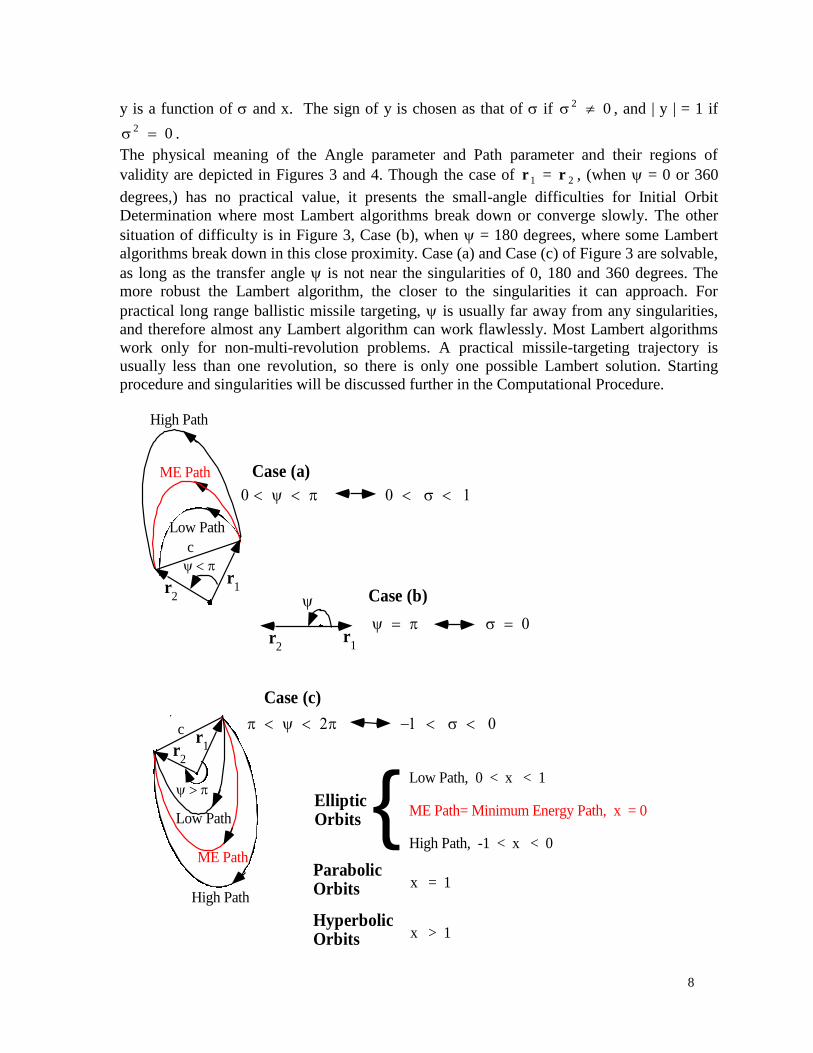
y is a function of and x. The sign of y is chosen as that of if 2 0 , and | y | = 1 if 2 0 .
The physical meaning of the Angle parameter and Path parameter and their regions of
validity are depicted in Figures 3 and 4. Though the case of 1r = 2r , (when = 0 or 360
degrees,) has no practical value, it presents the small-angle difficulties for Initial Orbit
Determination where most Lambert algorithms break down or converge slowly. The other
situation of difficulty is in Figure 3, Case (b), when = 180 degrees, where some Lambert
algorithms break down in this close proximity. Case (a) and Case (c) of Figure 3 are solvable,
as long as the transfer angle is not near the singularities of 0, 180 and 360 degrees. The
more robust the Lambert algorithm, the closer to the singularities it can approach. For
practical long range ballistic missile targeting, is usually far away from any singularities,
and therefore almost any Lambert algorithm can work flawlessly. Most Lambert algorithms
work only for non-multi-revolution problems. A practical missile-targeting trajectory is
usually less than one revolution, so there is only one possible Lambert solution. Starting
procedure and singularities will be discussed further in the Computational Procedure.
High Path
Low Path
ME Path
High Path
Low Path
ME Path
Low Path, 0 < x < 1
ME Path= Minimum Energy Path, x = 0
High Path, -1 < x < 0
r1r
2
r1r
2
r1
r2
c
c
EllipticOrbits {ParabolicOrbits x = 1
HyperbolicOrbits x > 1
Case (a)
Case (b)
Case (c)
9
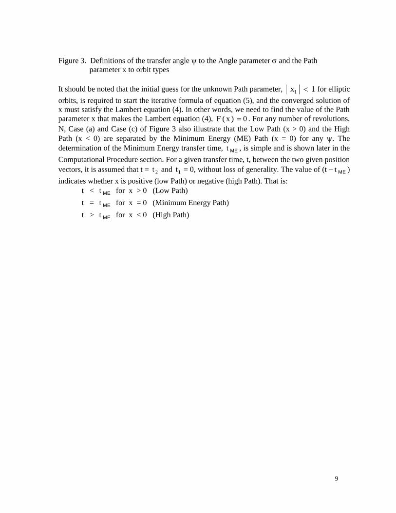
Figure 3. Definitions of the transfer angle to the Angle parameter and the Path
parameter x to orbit types
It should be noted that the initial guess for the unknown Path parameter, 1x 1 for elliptic
orbits, is required to start the iterative formula of equation (5), and the converged solution of
x must satisfy the Lambert equation (4). In other words, we need to find the value of the Path
parameter x that makes the Lambert equation (4), F ( x ) 0 . For any number of revolutions,
N, Case (a) and Case (c) of Figure 3 also illustrate that the Low Path (x > 0) and the High
Path (x < 0) are separated by the Minimum Energy (ME) Path (x = 0) for any . The
determination of the Minimum Energy transfer time, t ME , is simple and is shown later in the
Computational Procedure section. For a given transfer time, t, between the two given position
vectors, it is assumed that t = 2t and 1t = 0, without loss of generality. The value of (t t ME )
indicates whether x is positive (low Path) or negative (high Path). That is:
t < t ME for x > 0 (Low Path)
t = t ME for x = 0 (Minimum Energy Path)
t > t ME for x < 0 (High Path)
10
An
gle
par
amet
er
Path parameter
line
line
line
x
Path
parameter
x
High Path
High Path Low Path
Low Path
ME
Path
lin
e
ME
Path
lin
e
Elliptic Orbits, Multi-Revolution
vs x Regions of Solution
Ang
le p
aram
eter
line
line
line
No SolutionRegion
No SolutionRegion
No S
olu
tion
Reg
ion
No S
olu
tion
Reg
ion
No S
olu
tion
Reg
ion
No S
olu
tion
Reg
ion
No SolutionRegion
No SolutionRegion
constant line
Hig
h P
ath,
1 <
x <
0
Low
Pat
h,
0 <
x
<
1
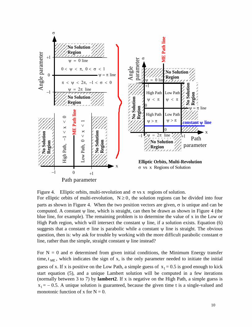
Figure 4. Elliptic orbits, multi-revolution and vs x regions of solution.
For elliptic orbits of multi-revolution, N 0 , the solution regions can be divided into four
parts as shown in Figure 4. When the two position vectors are given, is unique and can be
computed. A constant line, which is straight, can then be drawn as shown in Figure 4 (the
blue line, for example). The remaining problem is to determine the value of x in the Low or
High Path region, which will intersect the constant line, if a solution exists. Equation (6)
suggests that a constant line is parabolic while a constant line is straight. The obvious
question, then is: why ask for trouble by working with the more difficult parabolic constant
line, rather than the simple, straight constant line instead?
For N = 0 and determined from given initial conditions, the Minimum Energy transfer
time, t ME , which indicates the sign of x, is the only parameter needed to initiate the initial
guess of x. If x is positive on the Low Path, a simple guess of 1x = 0.5 is good enough to kick
start equation (5), and a unique Lambert solution will be computed in a few iterations
(normally between 3 to 7) by lambert2. If x is negative on the High Path, a simple guess is
1x = 0.5. A unique solution is guaranteed, because the given time t is a single-valued and
monotonic function of x for N = 0.
11
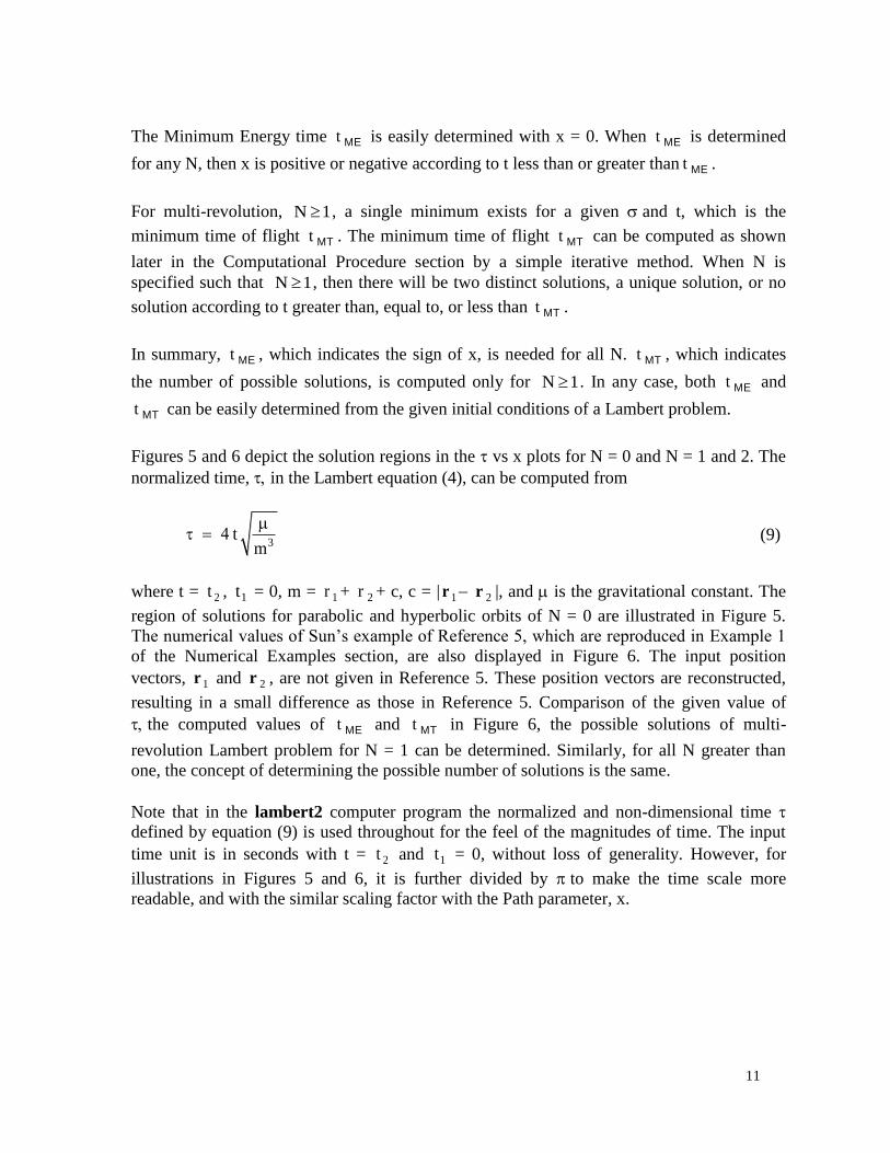
The Minimum Energy time t ME is easily determined with x = 0. When t ME is determined
for any N, then x is positive or negative according to t less than or greater than t ME .
For multi-revolution, N 1 , a single minimum exists for a given and t, which is the
minimum time of flight t MT . The minimum time of flight t MT can be computed as shown
later in the Computational Procedure section by a simple iterative method. When N is
specified such that N 1 , then there will be two distinct solutions, a unique solution, or no
solution according to t greater than, equal to, or less than t MT .
In summary, t ME , which indicates the sign of x, is needed for all N. t MT , which indicates
the number of possible solutions, is computed only for N 1 . In any case, both t ME and
t MT can be easily determined from the given initial conditions of a Lambert problem.
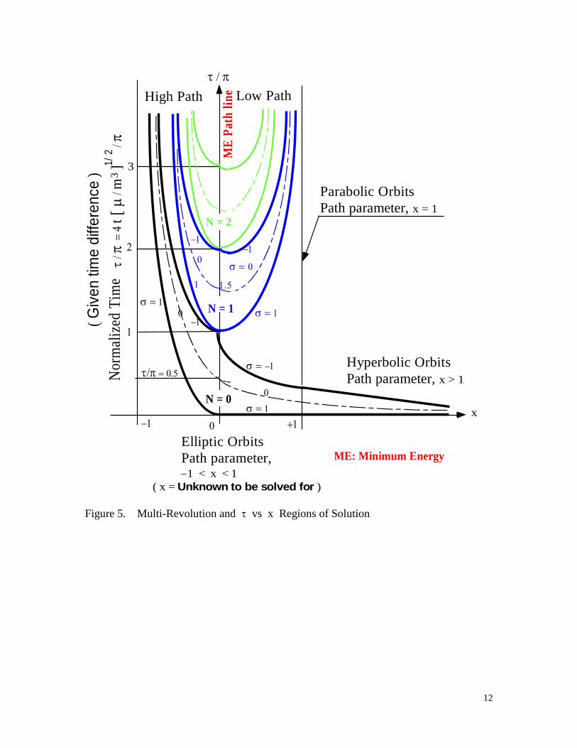
Figures 5 and 6 depict the solution regions in the vs x plots for N = 0 and N = 1 and 2. The
normalized time, in the Lambert equation (4), can be computed from
3t
m
(9)
where t = 2t , 1t = 0, m = 1r + 2r + c, c = | 1r 2r |, and is the gravitational constant. The
region of solutions for parabolic and hyperbolic orbits of N = 0 are illustrated in Figure 5.
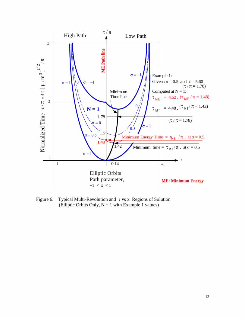
The numerical values of Sun’s example of Reference 5, which are reproduced in Example 1
of the Numerical Examples section, are also displayed in Figure 6. The input position
vectors, 1r and 2r , are not given in Reference 5. These position vectors are reconstructed,
resulting in a small difference as those in Reference 5. Comparison of the given value of
the computed values of t ME and t MT in Figure 6, the possible solutions of multi-
revolution Lambert problem for N = 1 can be determined. Similarly, for all N greater than
one, the concept of determining the possible number of solutions is the same.
Note that in the lambert2 computer program the normalized and non-dimensional time
defined by equation (9) is used throughout for the feel of the magnitudes of time. The input
time unit is in seconds with t = 2t and 1t = 0, without loss of generality. However, for
illustrations in Figures 5 and 6, it is further divided by to make the time scale more
readable, and with the similar scaling factor with the Path parameter, x.
12
Nor
mal
ized
Tim
e
Elliptic Orbits
Path parameter,1 < x < 1
x
High Path Low Path
Parabolic Orbits
Path parameter, x = 1
Hyperbolic Orbits
Path parameter, x > 1
3
3
1/
2
N = 1
N = 0
N = 2
ME: Minimum Energy
ME
Pat
h l
ine
t
m
]
( G
ive
n tim
e d
iffe
ren
ce )
( x = Unknown to be solved for )
Figure 5. Multi-Revolution and vs x Regions of Solution
13
Nor
mal
ized
Tim
e
3
1/
2
t
m
]
N = 1
High Path Low Path
ME
Path
lin
e
3
x
Minimum time = , at = 0.5M T
Minimum Energy Time = , at = 0.5M E
Minimum
Time line
Example 1:
Given : = 0.5 and = 5.60
Computed at N = 1:
= 4.62 ,
= 4.48 ,
M E
M T
= 1.78)
= 1.48)
= 1.42)
M E
M T
= 1.78)
ME: Minimum Energy
1.78
1.5
Elliptic Orbits
Path parameter,1 < x < 1
1.481.42
0.14
Figure 6. Typical Multi-Revolution and vs x Regions of Solution
(Elliptic Orbits Only, N = 1 with Example 1 values)
14
Computational Procedure
Conceptually, all Lambert formulations are similar to those described in the section General
Formulation of the Lambert Problem. Sun’s choice of the unknown variable, x, not only
allows for simple expressions of the Lambert equation (4) and its derivatives, F ( x ), F ( x )
and F ( x ) , but computable equations without ambiguity, and is applicable to multi-
revolution elliptic orbits that few can match. For elliptic orbits, x 1 must be strictly
enforced. Parabolic and hyperbolic orbits exist only for less than one revolution (N = 0) and
x 1 . These simple equations are included in Appendix A (reproduced from Reference 5)
and implemented in the source code. Since only elliptic orbits exist for multi-revolutions, a
physically understandable and sensibly bounded unknown parameter presents great
advantage over those formulations using other universal variables. Notice that Gooding of
Reference 7 defined this same unknown variable x as the unknown universal variable.
Furthermore the unknown (Path) parameter x is related to or identified by the physical Low
and High Paths separated by the Minimum Energy trajectory. Sun’s formulation for multi-
revolution elliptic transfer orbits can be reduced to the following steps:
0. Preliminary step: Before a Lambert algorithm is started, the transfer orbit to be determined
must be specified to be direct (inclination <= 90 degrees) or retrograde (inclination > 90
degrees). This is a hard-coded line in lambert2 instead of an input parameter in order to
keep the normal input parameters of two position vectors and two times. That is:
direct_torbit = 1.0 for direct transfer orbit with inclination <= 90 degrees
direct_torbit = -1.0 for retrograde transfer orbit with inclination > 90 degrees
A second parameter, , which controls or dictates the transfer angle to be less than or
greater than 180 degrees, is determined from the third component of the angular
momentum of the transfer orbit. That is:
1 2x )(0, 0,1) ( r r
This proper starting step allows the transfer angle defined in both 0 < and <
for either a direct or retrograde transfer orbit. Figure 2 shows four transfer
orbits, not the two transfer orbits, “short and long”, as described in many textbooks.
Again, the two solutions of “short and long” transfer orbits are misleading or incomplete,
and a user may unintentionally compute a transfer orbit of an unexpected inclination!
When the transfer angle, k and k is even or zero, transfer orbits are degenerate or
physically meaningless. They will not be treated. If k is odd, the transfer orbits are non-
degenerate and real, but there are infinite numbers. For this “singular” case, the inclination
of the transfer orbit must be specified first. The special case that the inclination is zero, the
transfer orbit is that of the Hohmann. For this reason, lambert2 only provides multi-
revolution Lambert solutions for real transfer orbits for all k The simple
Hohmann-type transfers, which are treated in many text books, are left as an exercise for
the readers.
15
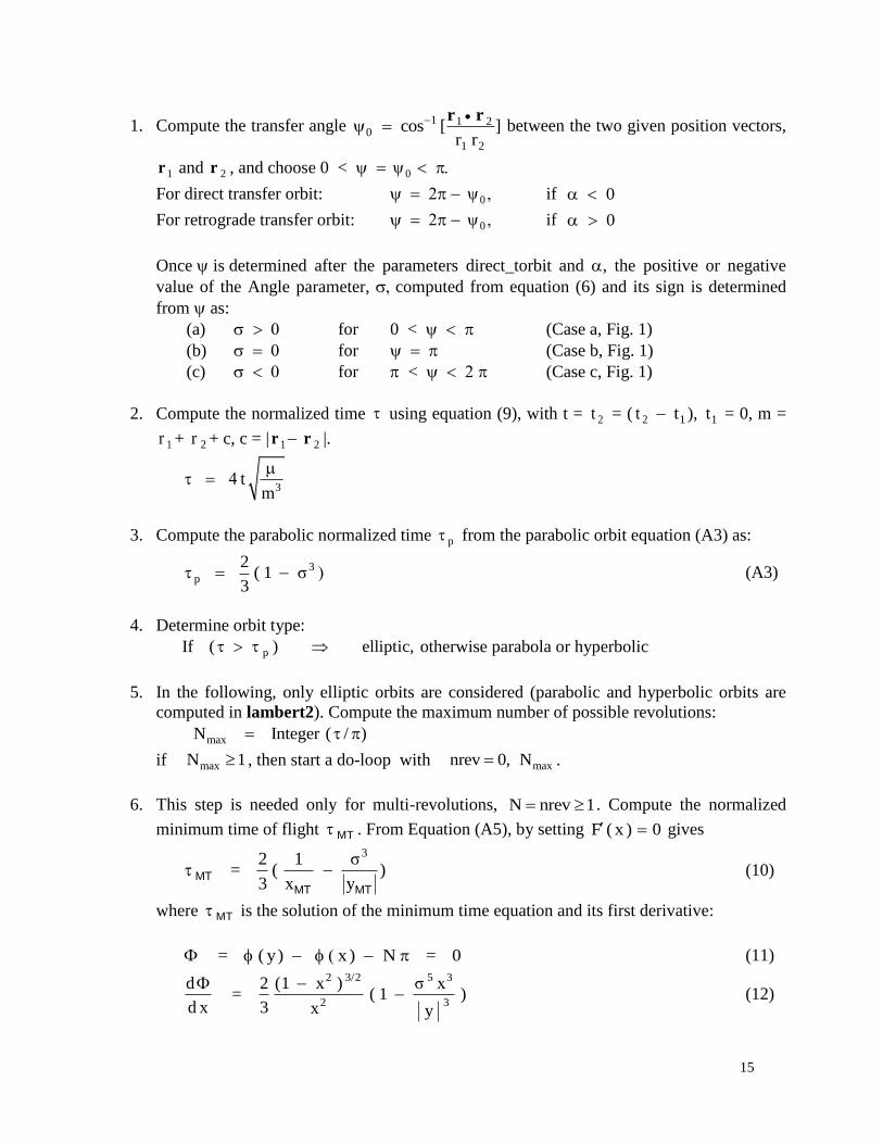
1. Compute the transfer angle 1 1 20
1 2
cos [ ]r r
r rbetween the two given position vectors,
1r and 2r , and choose 0 < 0
For direct transfer orbit: 0 if 0
For retrograde transfer orbit: 0 if 0
Onceisdetermined after the parameters direct_torbit and , the positive or negative
value of the Angle parameter, computed from equation (6) and its sign is determined
from as:
(a) for 0 < (Case a, Fig. 1)
(b) for (Case b, Fig. 1)
(c) for < (Case c, Fig. 1)
2. Compute the normalized time using equation (9), with t = 2t = ( 2t 1t ), 1t = 0, m =
1r + 2r + c, c = | 1r 2r |.
3t
m
3. Compute the parabolic normalized time p from the parabolic orbit equation (A3) as:
3p
2( 1 σ )
3 (A3)
4. Determine orbit type:
If p( ) elliptic, otherwise parabola or hyperbolic
5. In the following, only elliptic orbits are considered (parabolic and hyperbolic orbits are
computed in lambert2). Compute the maximum number of possible revolutions:
maxN Integer ( / )
if maxN 1 , then start a do-loop with maxnrev 0, N .
6. This step is needed only for multi-revolutions, N nrev 1 . Compute the normalized
minimum time of flight MT . From Equation (A5), by setting F ( x ) 0 gives
32 1 σ= ( )
3 x y MT
MT MT
(10)
where MT is the solution of the minimum time equation and its first derivative:
= ( y) x ) N = 0 (11)
2 3/2 5 3
2 3
d 2 (1 x ) σ x= ( 1 )
d x 3 x y
(12)
16
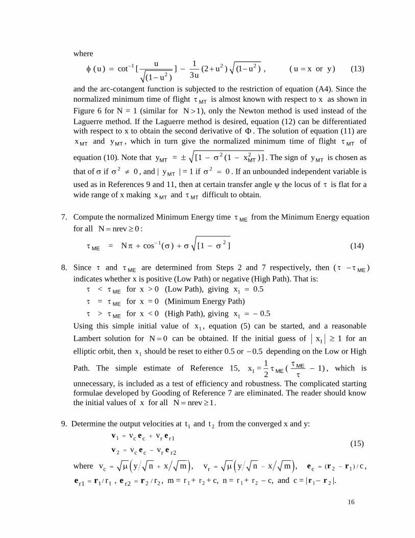
where
1 2 2
2
u 1(u ) cot [ ] (2 u ) (1 u ) , ( u x or y)
3u(1 u )
(13)
and the arc-cotangent function is subjected to the restriction of equation (A4). Since the
normalized minimum time of flight MT is almost known with respect to x as shown in
Figure 6 for N = 1 (similar for N 1 ), only the Newton method is used instead of the
Laguerre method. If the Laguerre method is desired, equation (12) can be differentiated
with respect to x to obtain the second derivative of . The solution of equation (11) are
x MT and yMT , which in turn give the normalized minimum time of flight MT of
equation (10). Note that 2 2y = [1 (1 x )] MT MT . The sign of yMT is chosen as
that of if 2 0 , and | yMT | = 1 if 2 0 . If an unbounded independent variable is
used as in References 9 and 11, then at certain transfer angle the locus of is flat for a
wide range of x making x MT and MT difficult to obtain.
7. Compute the normalized Minimum Energy time ME from the Minimum Energy equation
for all N nrev 0 :
21= N cos ( ) [1 ] ME (14)
8. Since and ME are determined from Steps 2 and 7 respectively, then ( ME )
indicates whether x is positive (Low Path) or negative (High Path). That is:
< ME for x > 0 (Low Path), giving 1x 0.5
= ME for x = 0 (Minimum Energy Path)
> ME for x < 0 (High Path), giving 1x 0.5
Using this simple initial value of 1x , equation (5) can be started, and a reasonable
Lambert solution for N 0 can be obtained. If the initial guess of 1x 1 for an
elliptic orbit, then 1x should be reset to either 0.5 or 0.5 depending on the Low or High
Path. The simple estimate of Reference 15, 1
1x = ( 1)
2
MEME , which is
unnecessary, is included as a test of efficiency and robustness. The complicated starting
formulae developed by Gooding of Reference 7 are eliminated. The reader should know
the initial values of x for all N nrev 1 .
9. Determine the output velocities at 1t and 2t from the converged x and y:
1
2
c c r r1
c c r r2
v v
v v
v e e
v e e (15)
where cv y n x m , rv y n x m , 2 1( ) /c c e r r ,
1 1/r1 re r , 2 2/r2 re r , m = 1r + 2r + c, n = 1r + 2r c, and c = | 1r 2r |.
17
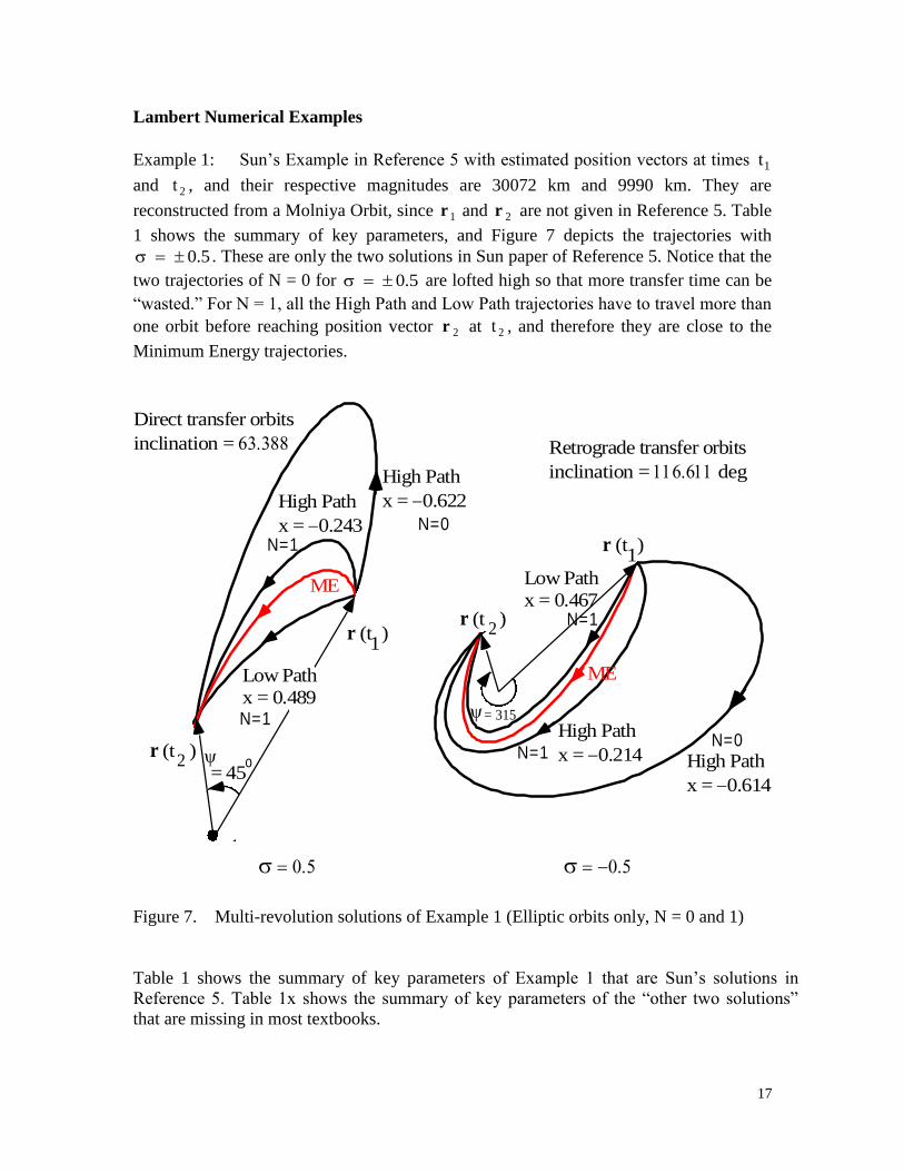
Lambert Numerical Examples
Example 1: Sun’s Example in Reference 5 with estimated position vectors at times 1t
and 2t , and their respective magnitudes are 30072 km and 9990 km. They are
reconstructed from a Molniya Orbit, since 1r and 2r are not given in Reference 5. Table
1 shows the summary of key parameters, and Figure 7 depicts the trajectories with
0.5 . These are only the two solutions in Sun paper of Reference 5. Notice that the
two trajectories of N = 0 for 0.5 are lofted high so that more transfer time can be
“wasted.” For N = 1, all the High Path and Low Path trajectories have to travel more than
one orbit before reaching position vector 2r at 2t , and therefore they are close to the
Minimum Energy trajectories.
o
ME
High Path
x = 0.622High Path
x = 0.243N=1
N=1
N=0
r (t )2
= 45o
r (t )1
Low Path
x = 0.489
ME
= 315
N=1
High Path
x = 0.214 High Path
x = 0.614
N=0
Low Path
x = 0.467N=1
r (t )2
r (t )1
Direct transfer orbits
inclination = Retrograde transfer orbits
inclination = deg
Figure 7. Multi-revolution solutions of Example 1 (Elliptic orbits only, N = 0 and 1)
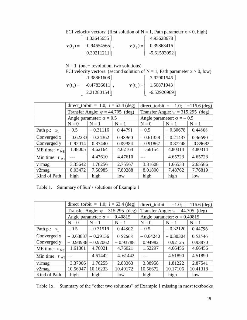
Table 1 shows the summary of key parameters of Example 1 that are Sun’s solutions in
Reference 5. Table 1x shows the summary of key parameters of the “other two solutions”
that are missing in most textbooks.
18
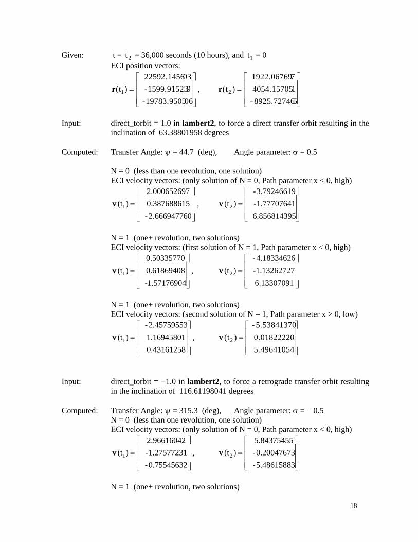
Given: t = 2t = 36,000 seconds (10 hours), and 1t = 0
ECI position vectors:
0619783.9505-
91599.91523-
0322592.1456
)(t1r ,
58925.72746-
14054.15705
71922.06769
)(t2r
Input: direct_torbit = 1.0 in lambert2, to force a direct transfer orbit resulting in the
inclination of 63.38801958 degrees
Computed: Transfer Angle: = 44.7 (deg), Angle parameter: = 0.5
N = 0 (less than one revolution, one solution)
ECI velocity vectors: (only solution of N = 0, Path parameter x < 0, high)
1
2.000652697
(t ) 0.387688615
-2.666947760
v , 2
-3.79246619
(t ) -1.77707641
6.856814395
v
N = 1 (one+ revolution, two solutions)
ECI velocity vectors: (first solution of N = 1, Path parameter x < 0, high)
1
0.50335770
(t ) 0.61869408
-1.57176904
v , 2
-4.18334626
(t ) -1.13262727
6.13307091
v
N = 1 (one+ revolution, two solutions)
ECI velocity vectors: (second solution of N = 1, Path parameter x > 0, low)
1
-2.45759553
(t ) 1.16945801
0.43161258
v ,
5.49641054
0.01822220
5.53841370-
)(t2v
Input: direct_torbit = 1.0 in lambert2, to force a retrograde transfer orbit resulting
in the inclination of 116.61198041 degrees
Computed: Transfer Angle: = 315.3 (deg), Angle parameter: = 0.5
N = 0 (less than one revolution, one solution)
ECI velocity vectors: (only solution of N = 0, Path parameter x < 0, high)
1
2.96616042
(t ) -1.27577231
-0.75545632
v , 2
5.84375455
(t ) -0.20047673
-5.48615883
v
N = 1 (one+ revolution, two solutions)
19
ECI velocity vectors: (first solution of N = 1, Path parameter x < 0, high)
1
1.33645655
(t ) -0.94654565
0.30211211
v , 2
4.93628678
(t ) 0.39863416
-5.61593092
v
N = 1 (one+ revolution, two solutions)
ECI velocity vectors: (second solution of N = 1, Path parameter x > 0, low)
1
-1.38861608
(t ) -0.47836611
2.21280154
v , 2
3.92901545
(t ) 1.50871943
-6.52926969
v
direct_torbit = 1.0; i = 63.4 (deg) direct_torbit = 1.0; i =116.6 (deg)
Transfer Angle: = 44.705 (deg) Transfer Angle: = 315.295 (deg)
Angle parameter: = 0.5 Angle parameter: = 0.5
N = 0 N = 1 N = 1 N = 0 N = 1 N = 1
Path p.: x1 0.5 0.31116 0.5 0.30678
Converged x 0.62233 0.24362 0.61358 0.21437
Converged y 0.92014 0.87440 0.91867 0.87248 0.89682
ME time: ME 1.48005 4.62164 4.62164 1.66154 4.80314 4.80314
Min time: MT --- 4.47610 4.47610 --- 4.65723 4.65723
v1mag 3.35642 1.76256 2.75567 3.31608 1.66533 2.65586
v2mag 8.03472 7.50985 7.80288 8.01800 7.48762 7.76819
Kind of Path high high low high high low
Table 1. Summary of Sun’s solutions of Example 1
direct_torbit = 1.0; i = 63.4 (deg) direct_torbit = 1.0; i =116.6 (deg)
Transfer Angle: = 315.295 (deg) Transfer Angle: = 44.705 (deg)
Angle parameter: = 0.40815 Angle parameter: = 0.40815
N = 0 N = 1 N = 1 N = 0 N = 1 N = 1
Path p.: x1 0.5 0.31919 0.5 0.32120
Converged x 0.63837 0.29136 0.64240 0.30304
Converged y 0.94936 0.92062 0.93788 0.94982 0.92125 0.93870
ME time: ME 1.61861 4.76021 4.76021 1.52297 4.66456 4.66456
Min time: MT --- 4.61442 4. 61442 --- 4.51890 4.51890
v1mag 3.37006 1.76255 2.83363 3.38958 1.81222 2.87541
v2mag 10.56047 10.16233 10.40172 10.56672 10.17106 10.41318
Kind of Path high high low high high low
Table 1x. Summary of the “other two solutions” of Example 1 missing in most textbooks
20
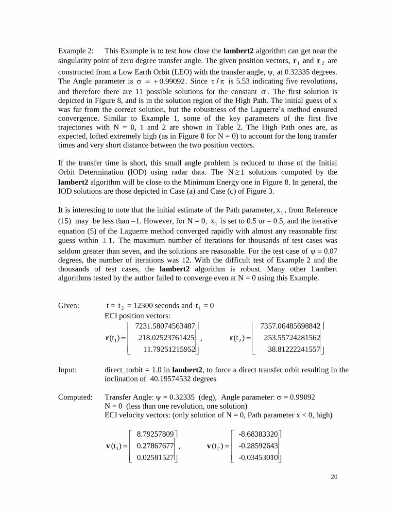
Example 2: This Example is to test how close the lambert2 algorithm can get near the
singularity point of zero degree transfer angle. The given position vectors, 1r and 2r are
constructed from a Low Earth Orbit (LEO) with the transfer angle, at 0.32335 degrees.
The Angle parameter is 0.99092 . Since / is 5.53 indicating five revolutions,
and therefore there are 11 possible solutions for the constant . The first solution is
depicted in Figure 8, and is in the solution region of the High Path. The initial guess of x
was far from the correct solution, but the robustness of the Laguerre’s method ensured
convergence. Similar to Example 1, some of the key parameters of the first five
trajectories with N = 0, 1 and 2 are shown in Table 2. The High Path ones are, as
expected, lofted extremely high (as in Figure 8 for N = 0) to account for the long transfer
times and very short distance between the two position vectors.
If the transfer time is short, this small angle problem is reduced to those of the Initial
Orbit Determination (IOD) using radar data. The N 1 solutions computed by the
lambert2 algorithm will be close to the Minimum Energy one in Figure 8. In general, the
IOD solutions are those depicted in Case (a) and Case (c) of Figure 3.
It is interesting to note that the initial estimate of the Path parameter, 1x , from Reference
(15) may be less than 1. However, for N = 0, 1x is set to 0.5 or 0.5, and the iterative
equation (5) of the Laguerre method converged rapidly with almost any reasonable first
guess within 1. The maximum number of iterations for thousands of test cases was
seldom greater than seven, and the solutions are reasonable. For the test case of 0.07
degrees, the number of iterations was 12. With the difficult test of Example 2 and the
thousands of test cases, the lambert2 algorithm is robust. Many other Lambert
algorithms tested by the author failed to converge even at N = 0 using this Example.
Given: t = 2t = 12300 seconds and 1t = 0
ECI position vectors:
1
7231.58074563487
(t ) 218.02523761425
11.79251215952
r , 2
7357.06485698842
(t ) 253.55724281562
38.81222241557
r
Input: direct_torbit = 1.0 in lambert2, to force a direct transfer orbit resulting in the
inclination of 40.19574532 degrees
Computed: Transfer Angle: = 0.32335 (deg), Angle parameter: = 0.99092
N = 0 (less than one revolution, one solution)
ECI velocity vectors: (only solution of N = 0, Path parameter x < 0, high)
1
8.79257809
(t ) 0.27867677
0.02581527
v , 2
-8.68383320
(t ) -0.28592643
-0.03453010
v
21
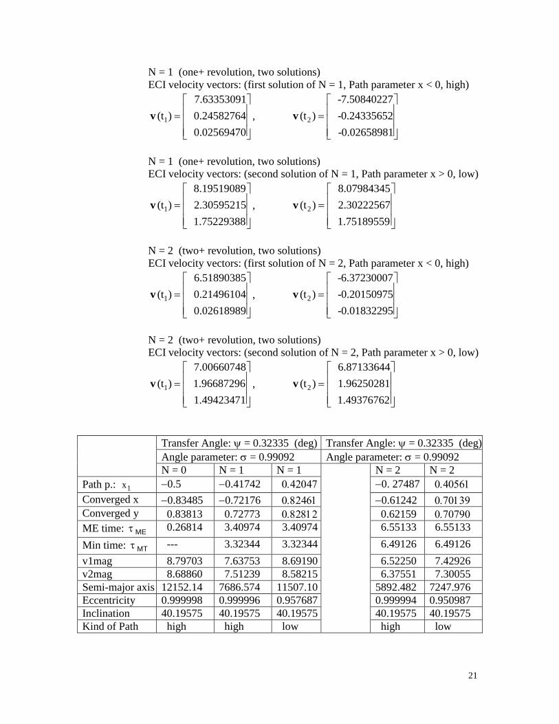
N = 1 (one+ revolution, two solutions)
ECI velocity vectors: (first solution of N = 1, Path parameter x < 0, high)
1
7.63353091
(t ) 0.24582764
0.02569470
v , 2
-7.50840227
(t ) -0.24335652
-0.02658981
v
N = 1 (one+ revolution, two solutions)
ECI velocity vectors: (second solution of N = 1, Path parameter x > 0, low)
1
8.19519089
(t ) 2.30595215
1.75229388
v , 2
8.07984345
(t ) 2.30222567
1.75189559
v
N = 2 (two+ revolution, two solutions)
ECI velocity vectors: (first solution of N = 2, Path parameter x < 0, high)
1
6.51890385
(t ) 0.21496104
0.02618989
v , 2
-6.37230007
(t ) -0.20150975
-0.01832295
v
N = 2 (two+ revolution, two solutions)
ECI velocity vectors: (second solution of N = 2, Path parameter x > 0, low)
1
7.00660748
(t ) 1.96687296
1.49423471
v , 2
6.87133644
(t ) 1.96250281
1.49376762
v
Transfer Angle: = 0.32335 (deg) Transfer Angle: = 0.32335 (deg)
Angle parameter: = 0.99092 Angle parameter: = 0.99092
N = 0 N = 1 N = 1 N = 2 N = 2
Path p.: 1x 0.5 0.41742 0. 27487
Converged x 0.83485 0.72176 0.61242
Converged y 0.83813 0.72773 0.62159
ME time: ME 0.26814 3.40974 3.40974 6.55133 6.55133
Min time: MT --- 3.32344 3.32344 6.49126 6.49126
v1mag 8.79703 7.63753 8.69190 6.52250 7.42926
v2mag 8.68860 7.51239 8.58215 6.37551 7.30055
Semi-major axis 12152.14 7686.574 11507.10 5892.482 7247.976
Eccentricity 0.999998 0.999996 0.957687 0.999994 0.950987
Inclination 40.19575 40.19575 40.19575 40.19575 40.19575
Kind of Path high high low high low
22
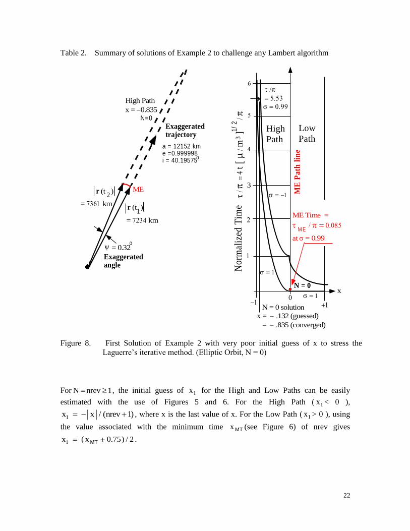
Table 2. Summary of solutions of Example 2 to challenge any Lambert algorithm
ME
High Path
x = 0.835
a = 12152 kme =0.999998i = 40.19575
o
N=0
= 0.32o
Exaggeratedangle
r (t )1
= km
= km
r (t )2
Nor
mal
ized
Tim
e3
1/
2
t
m
]
x = .132 (guessed)
= .835 (converged)
High
Path
Low
Path
3
N = 0
ME
Pat
h l
ine
x
ME Time =
M E
at = 0.99
N = 0 solution
x
Exaggeratedtrajectory
Figure 8. First Solution of Example 2 with very poor initial guess of x to stress the
Laguerre’s iterative method. (Elliptic Orbit, N = 0)
For N nrev 1 , the initial guess of 1x for the High and Low Paths can be easily
estimated with the use of Figures 5 and 6. For the High Path ( 1x < 0 ),
1x x / (nrev 1) , where x is the last value of x. For the Low Path ( 1x > 0 ), using
the value associated with the minimum time x MT (see Figure 6) of nrev gives
1x ( x 0.75) / 2 MT .

23
It is important to understand that the computed multi-revolution Lambert solutions of
N 1 may not agree with real motion. The user should make sure that the perigee radius
is greater than the Earth/central-body radius for real trajectories.
24
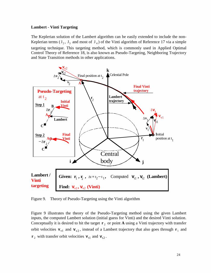
Lambert - Vinti Targeting
The Keplerian solution of the Lambert algorithm can be easily extended to include the non-
Keplerian terms ( 2J , 3J and most of 4J ) of the Vinti algorithm of Reference 17 via a simple
targeting technique. This targeting method, which is commonly used in Applied Optimal
Control Theory of Reference 18, is also known as Pseudo-Targeting, Neighboring Trajectory
and State Transition methods in other applications.
Celestial Pole
Final Vintitrajectory
k
ji
Final position at t
Central
body
v2
Lambert /
Vinti
targeting
Given: r , r , t = t t , Computed v , v (Lambert) 1 2 t1 t22 1
Find: v , v (Vinti)v1 v2
Lamberttrajectory
1r
2r
v2
v1 vt1
vt2
v1
2
1
2
C
A
B
C
A
InitialVinti
Lambert
Step 1
Step 2 Initialposition at t
A
vv1
vv2
Pseudo-Targeting
at t
v1
FinalVinti
r2
r2
Figure 9. Theory of Pseudo-Targeting using the Vinti algorithm
Figure 9 illustrates the theory of the Pseudo-Targeting method using the given Lambert
inputs, the computed Lambert solution (initial guess for Vinti) and the desired Vinti solution.
Conceptually it is desired to hit the target 2r or point A using a Vinti trajectory with transfer
orbit velocities v1v and v2v , instead of a Lambert trajectory that also goes through 1r and
2r with transfer orbit velocities t1v and t2v .
25
The initial inputs to the Vinti algorithm are the given position vector 1r , the computed
Lambert transfer orbit velocity t1v from the lambert2 algorithm, and the given times 1t and
2t . The initial Vinti trajectory, which includes 2J , 3J and most of 4J , ends at point B at 2t
as shown in Step 1 of Figure 9. To correct the position offset, the new target point C of Step
2 of Figure 9 is chosen exactly on the opposite side of point B with respect to point A. Along
the way, a 3x3 partial derivative matrix or a state transition matrix is constructed by varying
the transfer orbit velocity vector at 1t and the resulting changes in the position vector at 2t .
The small correction due to Vinti targeting results in the change of the transfer orbit velocity
by 1 v at 1t , which is the product of the inverse of the state transition matrix and the vector
difference of position 2r at 2t . The desired final Vinti trajectory can be obtained by
repeating Steps 1 and 2 of Figure 9. Upon convergence, the Keplerian solution of the
Lambert algorithm, ( t1v , t2v ), is replaced by the more accurate non-Keplerian solution of the
Vinti algorithm, ( v1v , v2v ).
The key to convergence and robustness is that the initial guess of the Keplerian transfer orbit
velocity t1v is reasonably close to the non-Keplerian solution of Vinti and the transition
matrix is computed by the accurate numerical partials technique of Reference 19. Let the
state vector at any time t be denoted as T
x r v , where r is the position vector and v
is the velocity vector. The iterative steps are summarized as follows:
1. Compute the Keplerian Lambert solution, ( t1v , t2v ) by the lambert2 algorithm.
2. Compute the nominal Vinti state vector T
* * *2 2 2
x r v at 2t using the given
position vector 1r , the nominal transfer orbit velocity 1*
t1v v , and the given times 1t
and 2t as inputs to the Vinti algorithm.
3. Evaluate the nominal differential correction of the position vector (point A point B) at
2t as
*
2 2 2 r r r
4. Compute the transition matrix, T, by accurate numerical partials. Using the Vinti
algorithm successively for three times in the neighborhood of the nominal trajectory by
perturbing one at a time, each of the three Cartesian components of the nominal transfer
orbit velocity vector *1v at 1t with a step-size of ih , ( i = 1, 2, 3 ). That is
T* * *
1 1 11 11i 1i ih v v v v
The step-size ih is usually set to 610
only for the thi Cartesian component. For j i ,
then jh 0 . Using the accurate numerical partials technique, each of the thi neighboring
trajectory invokes four more trajectories with the four step-sizes of ih 2 , ih 2 ,
ih 2 , ih 2 , where a good choice of is 0.5. Let the corresponding four position
26
vectors 2ir at 2t computed by the Vinti algorithm be denoted as 1y , 2y , 3y and 4y .
The three partial derivatives of the thi column of T is given by
33 4 1 2
2
2i
*1i i
h
r y y y y
v
The 3 x 3 transition matrix can be approximated as
1 11 12 13
2 21 22 23
* * * *
r r r rT
v v v v
In computing T, 12 predictions by the Vinti algorithm are required (four for each i).
5. Update the nominal 1*
v at 1t as
1
1 1 1
* * *1 2new old old
v v v v T r
Steps 2 to 5 are repeated until the magnitude of 2r is reduced to an acceptably small
value (eg., 1210
km). Note that in Step 2, the new nominal transfer orbit velocity is
1 1* *
newv v after the first iteration. Normally only three iterations are required. Upon
convergence, the desired Vinti velocities of the transfer orbit are 1*
v1 vv and
2*
v2 vv .
The accurate numerical partials technique of computing the state transition matrix T requires
four times more evaluations than the tradition partial derivative method. However, the rate of
convergence is much faster and the choice of the step-size ih is more forgiving, and
therefore improves robustness. The Lambert and Vinti trajectories are both analytic. The non-
Keplerian solution of the Lambert-Vinti targeting that includes the gravitational potential
terms of 2J , 3J and most of 4J can be computed almost instantly. If higher accuracy is
desired, then the nominal trajectory and/or the state transition matrix may be computed by
numerical integration with all the desired perturbed accelerations. The resulting non-
Keplerian velocities of the transfer orbit by Lambert-Numerical targeting will be more
accurate than that of the Lambert-Vinti targeting, but at the expense of considerably more
CPU times.
27
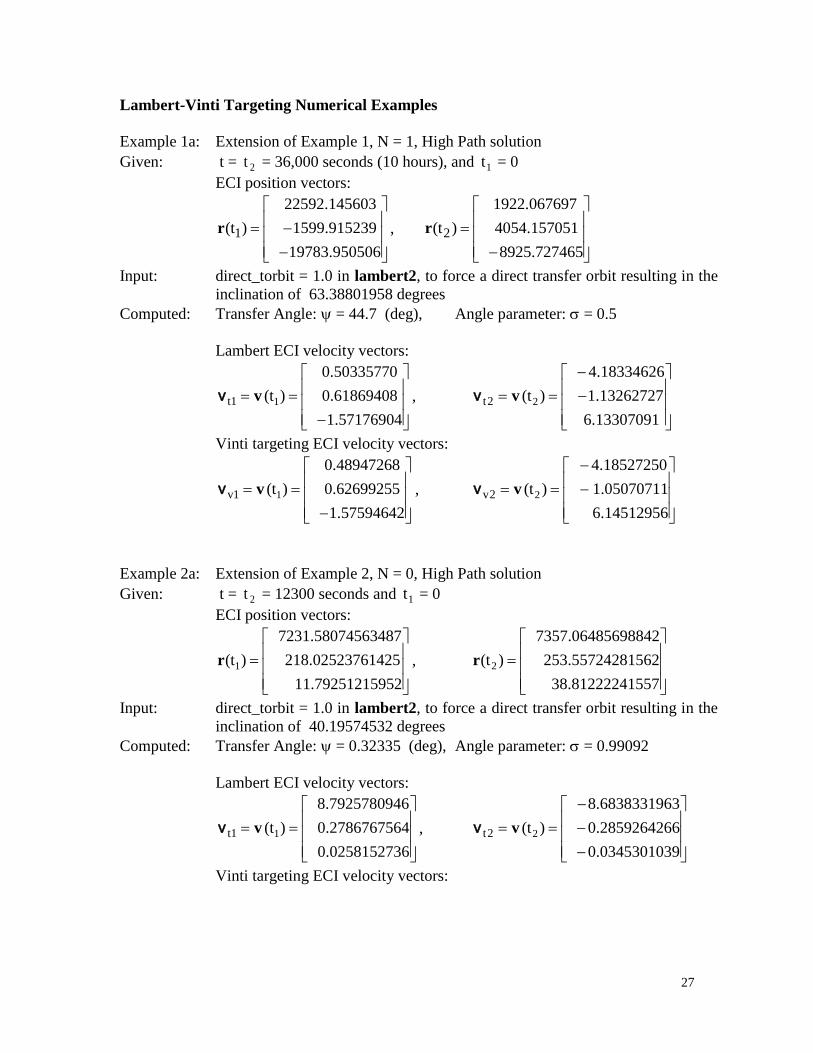
Lambert-Vinti Targeting Numerical Examples
Example 1a: Extension of Example 1, N = 1, High Path solution
Given: t = 2t = 36,000 seconds (10 hours), and 1t = 0
ECI position vectors:
1
22592.145603
(t ) 1599.915239
19783.950506
r , 2
1922.067697
(t ) 4054.157051
8925.727465
r
Input: direct_torbit = 1.0 in lambert2, to force a direct transfer orbit resulting in the
inclination of 63.38801958 degrees
Computed: Transfer Angle: = 44.7 (deg), Angle parameter: = 0.5
Lambert ECI velocity vectors:
1t1
0.50335770
(t ) 0.61869408
1.57176904
vv , 2t2
4.18334626
(t ) 1.13262727
6.13307091
vv
Vinti targeting ECI velocity vectors:
1v1
0.48947268
(t ) 0.62699255
1.57594642
vv , 2v2
4.18527250
(t ) 1.05070711
6.14512956
vv
Example 2a: Extension of Example 2, N = 0, High Path solution
Given: t = 2t = 12300 seconds and 1t = 0
ECI position vectors:
1
7231.58074563487
(t ) 218.02523761425
11.79251215952
r , 2
7357.06485698842
(t ) 253.55724281562
38.81222241557
r
Input: direct_torbit = 1.0 in lambert2, to force a direct transfer orbit resulting in the
inclination of 40.19574532 degrees
Computed: Transfer Angle: = 0.32335 (deg), Angle parameter: = 0.99092
Lambert ECI velocity vectors:
1t1
8.7925780946
(t ) 0.2786767564
0.0258152736
vv , 2t2
8.6838331963
(t ) 0.2859264266
0.0345301039
vv
Vinti targeting ECI velocity vectors:
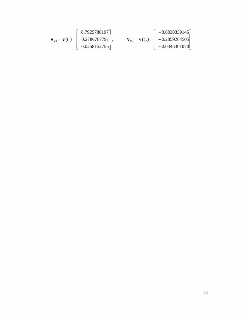
28
1v1
8.7925788197
(t ) 0.2786767791
0.0258152755
vv , 2v2
8.6838339145
(t ) 0.2859264505
0.0345301070
vv
29
Conclusions
The DerAstrodynamics lambert2 algorithm can also be used for interplanetary trajectories, if
the gravitational constant is replaced by that of the Sun. The four recommendations for
further works by Klumpp (Reference 10) in 1991 are accomplished by the elegant
formulation of Professor Sun of Reference 5 and the “modified” iterative method of
Laguerre. The complicated starting formulae, third derivative evaluation for the Halley
method, and the convergence testing developed by Gooding of Reference 7 are eliminated.
In summary:
1. No starter algorithm is needed. The initial guess of the unknown iterative parameter x
for N = 0 can be simply set to 0.5 . For any N, x is positive or negative according to
the given time t = ( 2t 1t ), less than or greater than the Minimum Energy time t ME .
2. No averaging and/or lower and upper limits are computed or needed.
3. No Newton method is used; otherwise the algorithm will not be robust.
4. No fixed higher-order/degree iteration equation is designated, but the degree of the
polynomial equation of the Laguerre method is allowed to vary.
Despite Conway’s claim of robustness by using a “fixed” fifth-degree iterative equation of
Laguerre for solving the Kepler equation (Reference 13), it is shown to fail in the
DerAstrodynamics kepler1 examples. In fact, the “fixed” fifth-degree iterative equation of
Laguerre failed to predict a correct Kepler solution approximately one out of a thousand
using the initial state vectors from any day of the NORAD Space Catalog and prediction
times of almost any number of days. Similarly Halley’s cubic iteration process cannot
guarantee robustness, because it is a “fixed” cubic iterative equation.
Since the lambert2 algorithm has the same independent “universal variable” parameter x as
that of Gooding, strictly speaking Sun’s formulation is universal.
The Primer Vector approach of Reference 11 has difficulties in the initial guess and
convergence due to the unbounded independent parameter, and therefore solutions are not
guaranteed. The Series Reversion/Inversion method of Reference 12 presents implementation
difficulty of matrix manipulations, and is limited to less than one revolution. Instead of
solving a Lambert equation, References 8 and 9 deduce the unknown from a cubic Kepler
equation. Since the unknown is unbounded, solutions are not guaranteed. None of these
Lambert algorithms and many others can guarantee accuracy and robustness.
The Gooding Lambert algorithm may be the best as suggested by Klumpp of JPL in 1991.
The superior lambert2 algorithm, which has eliminated all the difficulties of the Gooding
Lambert algorithm, is the fastest, most accurate and robust, multi-revolution Lambert
algorithm in 2011 and beyond. Using the analytic DerAstrodynamics vinti algorithm and
simple targeting, the Keplerian solution of the lambert2 algorithm can be extended to
include the non-Keplerian terms of Vinti to achieve orders of magnitude accuracy
improvement.
30
Appendix A
The Lambert equation from Reference 5 can be expressed as:
1 1 2 2
2 3 2 2
1 1 2 2
2 3 2 2
3
1 x ycot [ ] cot [ ] x (1 x ) y (1 y ) N
(1 x ) (1 x ) (1 y )
( elliptic, x 1 ) (A1)
1 x ycoth [ ] coth [ ] x (x 1) y (y 1)
F(x) = (x 1) (x 1) (y 1)
( hyperbolic, x 1 ) (A2)
2( 1 σ )
3
( parabolic,
x 1) (A3)
1 1
2 2
x y0 cot [ ] , cot [ ]
2 2(1 x ) (1 y )
(A4)
The first and second derivatives of the Lambert equation (A1) for multi-revolution
elliptic trajectories can be expressed as:
3
2
1 xF ( x ) = = 3x 2(1 )
x y(1 x )
(A5)
2 32 5
2 2 3
1 xF ( x ) = = (1 4x )F ( x ) 2(1 )
x x (1 x ) y
(A6)
where 2 2y = [1 (1 x )] . The sign of y is chosen as that of if 2 0 , and | y |
= 1 if 2 0 . When N is specified and is given, the multi-revolution elliptic orbits
equations (A1), (A5) and (A6) can be substituted into the Laguerre’s iterative formula of
equation (5). Together with the guessed value of 1x in Step 8 of the Computational
Procedure and any value of n of the polynomial degree (starting at n = 2), the lambert2
algorithm can be initiated for any revolution N 0 . When x and y are substituted into
equation (A1), equation (A4) must be strictly enforced, otherwise F ( x ) will be computed
incorrectly.
31
References
1. Gauss, C.F. "Theoria motas corporum coelestium in section-ibus conic solem
ambientium", 1809, (English translation by C.H. Davis, Little, Brown & Co., Boston,
1857.
2. Battin, R.H. "An Introduction to The Mathematics and Methods of Astrodynamics",
American Institute of Aeronautics and Astronautics, Education Series, 1987.
3. Godal, T. "Method for Determining the Initial Velocity Vector Corresponding to a Given
Time of Free Flight Transfer Between Given Points in a Simple Gravitational Field.”
Astronautik, Vol. 2, 1961, pp 183-186.
4. Vinh, N.X."Invariance in the Lambert’s Problem,” Lecture Notes, The University of
Michigan, 1977.
5. Sun, F.T. "On the Minimum Time Trajectory and Multiple Solutions of Lambert’s
Problem", AAS/AIAA Astrodynamics Conference, Province Town, Massachusetts, AAS
79-164, June 25-27, 1979.
6. Lancaster, E.R., Blanchard, R.C. "A Unified Form of Lambert’s Theorem", NASA TN D
5368, Goddard Space Flight Center, Greenbelt MD, 1969.
7. Gooding, R.H. "A Procedure for the Solution of Lambert’s Orbital Boundary-Value
Problem", Celestial Mechanics and Dynamic Astronomy 48, Number 2, 1990.
8. Battin, R.H., Vaughan, R.H. "An Elegant Lambert Algorithm", Journal of Guidance and
Control, Vol. 7, pp. 662-670, 1984.
9. Loechler, L.A. "An Elegant Lambert Algorithm for Multiple Revolution Orbits", Master
of Science Thesis, MIT, 1988.
http://dspace.mit.edu/bitstream/handle/1721.1/34998/20403052.pdf?sequence=1
10. Klumpp, A., "Performance Comparison of Lambert and Kepler Algorithms", Interoffice
Memorandum, JPL, 1999 February.
11. Pressing, J.E., "A Class of Optimal Two-Impulse Rendezvous Using Multiple-Revolution
Lambert Solutions", The Journal of the Astronautical Sciences, Vol. 48, Nos 2 and 3,
April-September 2000.
12. Thorne, J.D., Bain, R.D., "Series Reversion/Inversion of Lambert’s Time Function", The
Journal of the Astronautical Sciences, Vol. 43, No. 3, 1995.
13. Pressing, J.E., Conway, B.A., "Orbital Mechanics", Oxford University, 1993.
14. Tewari, A., "Atmospheric and Space Flight Dynamics", Birkhauser, 2007.
15. Monuki, A.T. "Deviation of x-iterator and comparison of Lambert Routines", TRW
7121.3-173, May 7,1973.
16. Gooding, R.H. "A New Procedure for the Solution of the Classical Problem of Minimal
Orbit Determination from three Lines of Sight", Celestial Mechanics and Dynamic
Astronomy 66, Vol 4, 1997.
17. Vinti, J.P., “Orbital and Celestial Mechanics”, AIAA, Volume 177,1998.
18. Bryson, A.E., Ho, Y.C., "Applied Optimal Control", Hemisphere Publishing, New York,
1975.
19. Danchick, R., "Accurate Numerical Partials with Applications to Maximum Likelihood
Methods ", Internal Rand Report, 1975.